arX

iv:1

403.

4687

v2 [

quan

t-ph

] 1

6 Se

p 20

14

Equivalence of wave-particle duality to entropic uncertainty

Patrick J. Coles, Jędrzej Kaniewski, and Stephanie WehnerCentre for Quantum Technologies, National University of Singapore, 2 Science Drive 3, 117543 Singapore

Interferometers capture a basic mystery of quantum mechanics: a single particle can exhibit wavebehavior, yet that wave behavior disappears when one tries to determine the particle’s path insidethe interferometer. This idea has been formulated quantitively as an inequality, e.g., by Englertand Jaeger, Shimony, and Vaidman, which upper bounds the sum of the interference visibility andthe path distinguishability. Such wave-particle duality relations (WPDRs) are often thought tobe conceptually inequivalent to Heisenberg’s uncertainty principle, although this has been debated.Here we show that WPDRs correspond precisely to a modern formulation of the uncertainty principlein terms of entropies, namely the min- and max-entropies. This observation unifies two fundamentalconcepts in quantum mechanics. Furthermore, it leads to a robust framework for deriving novelWPDRs by applying entropic uncertainty relations to interferometric models. As an illustration,we derive a novel relation that captures the coherence in a quantum beam splitter.

INTRODUCTION

When Feynman discussed the two-path interferome-ter in his famous lectures [1], he noted that quantumsystems (quantons) display the behavior of both wavesand particles and that there is a sort of competition be-tween seeing the wave behavior versus the particle behav-ior. That is, when the observer tries harder to figure outwhich path of the interferometer the quanton takes, thewave-like interference becomes less visible. This tradeoffis commonly called wave-particle duality (WPD). Feyn-man further noted that this is “a phenomenon which isimpossible ... to explain in any classical way, and whichhas in it the heart of quantum mechanics. In reality, itcontains the only mystery [of quantum mechanics].”

Many quantitative statements of this idea, so-calledwave-particle duality relations (WPDRs), have been for-mulated [2–13]. Such relations typically consider theMach-Zehnder interferometer for single photons, seeFig. 1. For example, a well-known formulation provenindependently by Englert [2] and Jaeger et al. [3] quanti-fies the wave behavior by fringe visibility V , and particlebehavior by the distinguishability of the photon’s path,D. (See below for precise definitions; the idea is that“waves” have a definite phase, while “particles” have adefinite location, hence V and D respectively quantifyhow definite the phase and location are inside the inter-ferometer.) They found the tradeoff:

D2 + V26 1 (1)

which implies V = 0 when D = 1 (full particle behaviormeans no wave behavior) and vice-versa, and also treatsthe intermediate case of partial distinguishability.

It has been debated, particularly around the mid-1990’s [14–16], whether the WPD principle, closely re-lated to Bohr’s complementarity principle [17], is equiva-lent to another fundamental quantum idea with no clas-sical analog: Heisenberg’s uncertainty principle [18]. Thelatter states that there are certain pairs of observables,such as position and momentum or two orthogonal com-ponents of spin angular momentum, that cannot simul-taneously be known or jointly measured. Likewise there

are many quantitative statements of this idea, known asuncertainty relations (URs) (see, e.g., [19–29]), and mod-ern formulations typically use entropy instead of stan-dard deviation as the uncertainty measure, so-called en-tropic uncertainty relations (EURs) [24]. This is becausethe standard deviation formulation suffers from trivialbounds when applied to finite-dimensional systems [21],whereas the entropic formulation not only fixes this weak-ness but also implies the standard deviation relation [22]and has relevance to information-processing tasks.

At present the debate regarding wave-particle dual-ity and uncertainty remains unresolved, to our knowl-edge. Yet Feynman’s quote seems to suggest a beliefthat quantum mechanics has but one mystery and nottwo separate ones. In this article we confirm this beliefby showing a quantitative connection between URs andWPDRs, demonstrating that URs and WPDRs capturethe same underlying physics; see also [30, 31] for somepartial progress along these lines. This may come as asurprise, since Englert [2] originally argued that (1) “doesnot make use of Heisenberg’s uncertainty relation in anyform”. To be fair, the uncertainty relation that we showis equivalent to (1) was not known at the time of En-glert’s paper, and was only recently discovered [25–29].Specifically, we will consider EURs, where the particularentropies that are relevant to (1) are the so-called min-and max-entropies used in cryptography [32].

In what follows we provide a general framework forderiving and discussing WPDRs - a framework that isultimately based on the entropic uncertainty principle.We illustrate our framework by showing that several dif-ferent WPDRs from the literature are in fact particu-lar examples of EURs. Making this connection not onlyunifies two fundamental concepts in quantum mechanics,but also implies that novel WPDRs can be derived sim-ply by applying already-proven EURs. Indeed we use ourframework to derive a novel WPDR for an exotic scenarioinvolving a “quantum beam splitter” [33–36], where test-ing our WPDR would allow the experimenter to verifythe beam splitter’s quantum coherence (see (17)).

We emphasize that the framework provided by EURsis highly robust, and entropies have well-characterized

2

BS1BS2

|0〉

|1〉

D0

D1

E1

E2

t1 t2

φ

Which path (Z)? Which phase (W )?

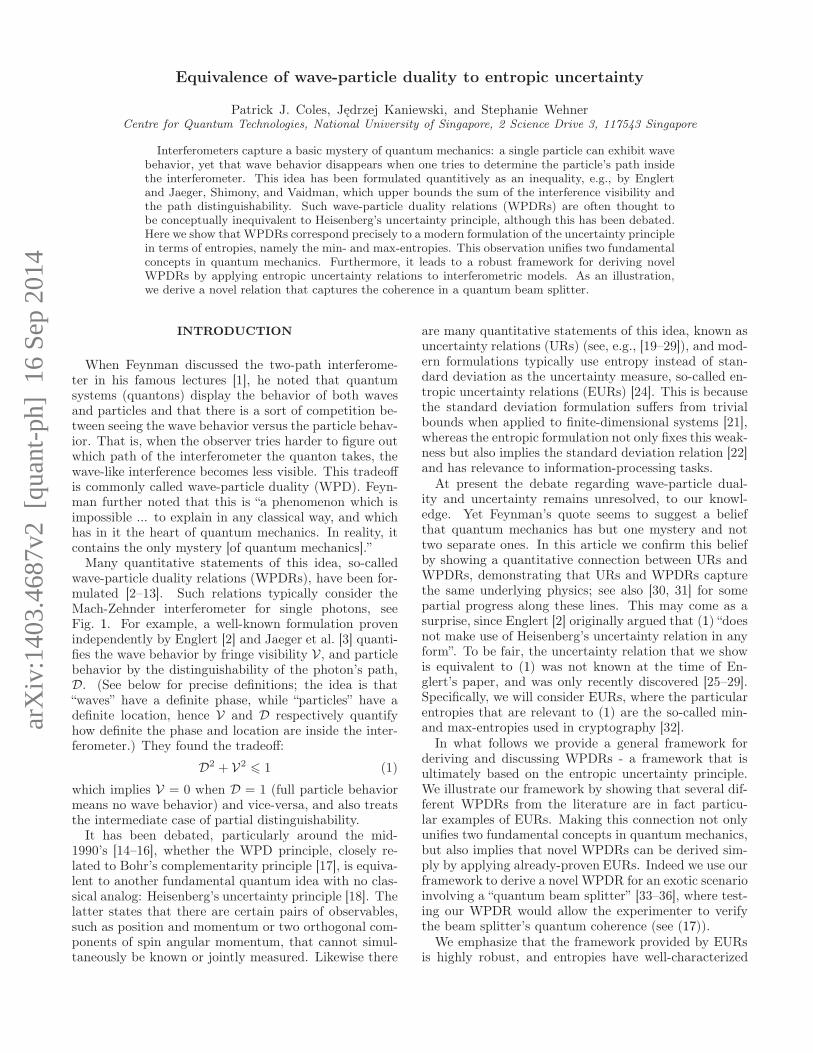
FIG. 1: Mach-Zehnder interferometer for single photons.Passing through the first beam splitter creates a superpo-sition of which-path states, |0〉 and |1〉, at time t1, then thesystem interacts with an environment E = E1E2. Finally attime t2 a phase shift φ is applied to the lower arm and thetwo beams are recombined on a second beam splitter. (Whilethis is the typical setup, our framework also allows E to playa more general role, e.g., being correlated to the photon be-fore it enters the MZI.) Our complementary guessing gameproceeds as follows. In one game (colored red) Alice tries toguess which of the two paths the photon took given that shehas access to a portion of E denoted E1, which could be, e.g.,a gas of atoms whose internal states record information aboutthe presence of a photon. In the other game (colored blue),one of two phases, φ = φ0 or φ = φ0 + π, is randomly appliedto the lower interferometer arm and Alice tries to guess φ

given that she has access to a different portion of E denotedE2, which could be, e.g., the photon’s polarisation. We arguethat WPDRs impose fundamental trade-offs on Alice’s abilityto win these two games.

statistical meanings. Note that current approaches toderiving WPDRs often involve brute force calculation ofthe quantities one aims to bound; there is no general,elegant method currently in use. Our approach simplyinvolves judicial application of the relevant uncertaintyrelation. What’s more, we emphasize that uncertaintyrelations can be applied to interferometers in two differ-ent ways. One involves preparation uncertainty, whichsays that a quantum state cannot be prepared havinglow uncertainty for two complementary observables, andit turns out this is the principle relevant to the originalpresentation of (1) in [2]. The other involves measure-ment uncertainty, which says that two complementaryobservables cannot be jointly measured [7, 31], and wediscuss why this principle is actually what was tested insome recent interferometry experiments [34, 37].

RESULTS

Framework

Guessing games.—We argue that a natural and pow-erful way to think of wave-particle duality is in terms ofguessing games, and one’s ability to win such games isquantified by entropic quantities. Specifically we consider

complementary guessing games, where Alice is asked toguess one of two complementary observables - a modernparadigm for discussing the uncertainty principle. In theMach-Zehnder interferometer (MZI), see Fig. 1, this cor-responds to either guessing which path the photon took,or which phase was applied inside the interferometer.The which-path and which-phase observables are com-plementary and hence the uncertainty principle gives afundamental restriction stating that Alice cannot be ableto guess both observables.

Binary interferometers.—Our framework treats thiscomplementary guessing game for binary interferome-ters. By binary, we mean any interferometer where thereare only two interfering paths, i.e., all other paths areclassically distinguishable (from each other and from thetwo interfering paths). In addition to the MZI, this in-cludes as special cases, e.g., the Franson interferometer[38] (see Fig. 2) and the double slit interferometer (seeFig. 3). Note that binary interferometers go beyond in-terferometers with two physical paths. For example, inthe Franson interferometer there are four possible pathsbut post-selecting on coincidence counts discards two ofthese paths, which are irrelevant to the interference any-way.

Particle observable.—Now we link wave and particlebehavior to knowledge of complementary observables. Inthe case of particle behavior, the intuition is that parti-cles have a well-defined spatial location, hence “particle-ness” should be connected to knowledge of the path insideinterferometer. For binary interferometers, there may bemore than two physical paths but only two of these areinterfering. Hence we only consider the two-dimensionalsubspace associated with the two which-path states of in-terest, denoted |0〉 and |1〉. This subspace can be thoughtof as an effective qubit, denoted Q, and the standard ba-sis of this qubit:

which-path: Z = |0〉, |1〉 (2)

corresponds precisely to the which-path observable. Forexample, in the double slit (Fig. 3), |0〉 and |1〉 are thepure states that one would obtain at the slit exit fromblocking the bottom and top slits respectively.

Wave observable.—Wave behavior is traditionally asso-ciated with having a large amplitude of intensity oscilla-tions at the interferometer output. Indeed this has beenquantified by the so-called fringe visibility, see (7), butto apply the uncertainty principle we need to relate wavebehavior to an observable inside the interferometer. Clas-sical waves (e.g., water waves) are often modelled as hav-ing a well-defined phase and being spatially delocalized.The analog in our context corresponds to the quantonbeing in a equally-weighted superposition of which-pathstates. Hence eigenstates of the “wave observable” shouldlive in the XY plane of the Bloch sphere, so we considerobservables on qubit Q (the interfering subspace) of the

3

DB0

DB1

φB|L〉

|S〉

Which phase,φ = φA + φB?

sourceE1

E2

DA0

DA1

φA|L〉

|S〉

Which path,

|LL〉 or |SS〉?

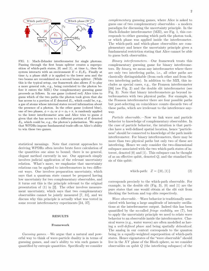
FIG. 2: In the Franson interferometer, the “quanton” consistsof two photons. That is, a source produces time-energy entan-gled photons that each head separately towards a MZI thatcontains a long arm (depicted with extra loops) and a shortarm. A simple model considers the four-dimensional Hilbertspace associated with the four possible paths: |SS〉, |SL〉,|LS〉, and |LL〉 with S = short path, L = long path. Two ofthese dimensions are post-selected away by considering onlycoincidence counts, i.e., the photons arriving at the same timeis inconsistent with the |SL〉 and |LS〉 paths. The remainingpaths, |0〉 := |SS〉 and |1〉 := |LL〉, are indistinguishable inthe special case of perfect visibility and they produce inter-ference fringes as one varies φ := φA + φB . Namely, theintensity of coincidence counts at detector pair (DA

0 , DB0 ) os-

cillates with φ. Interaction with an environment system, ormaking the beam splitters asymmetric, may allow one to par-tially distinguish between |SS〉 and |LL〉, and our entropicuncertainty framework can be applied to derive a tradeoff,e.g., of the form of (1). This tradeoff captures the idea thatAlice can either guess which path (|SS〉 vs. |LL〉) or whichphase (φ = φ0 vs. φ = φ0 + π), but she cannot do both (evenif she extracts information from other systems E1 and E2).

form

which-phase: W = |w±〉, |w±〉 =1√2(|0〉 ± eiφ0 |1〉).

(3)In terms of the guessing game, guessing the value of thewave (or which-phase) observable corresponds to guess-ing whether a phase of φ = φ0 or φ = φ0+π was appliedinside the interferometer (see, e.g., Fig 1). While φ0 is ageneric phase, its precise value will be singled out by theparticular experimental setup. When the experimentermeasures fringe visibility this corresponds to varying φ0to find the largest intensity contrast, and mathematicallywe model this by minimizing the uncertainty within theXY plane, see (4b).

Entropic View

Our entropic view associates a kind of behavior withthe availability of a kind of information, or lack of be-havior with missing information, as follows:

lack of particle behavior:Hmin(Z|E1) (4a)

lack of wave behavior: minW∈XY

Hmax(W |E2) (4b)

where Hmin and Hmax are the min- and max-entropies,defined below in (6), which are commonly used in quan-tum information theory, Z is the which-path observablein (2), W is the which-phase observable in (3) (whoseuncertainty we optimize over the XY plane of the Blochsphere), and E1 and E2 are some other quantum sys-tems that contain information and measuring these sys-tems may help to reveal the behavior (e.g., E1 could be awhich-path detector and E2 could be the quanton’s inter-nal degree of freedom). Note that we use the same sym-bols (Z, W , etc.) for the observables as for the randomvariables they give rise to. Full behavior (no behavior) ofsome kind corresponds to the associated entropy in (4)being zero (one). We formulate our general WPDR as

Hmin(Z|E1) + minW∈XY

Hmax(W |E2) > 1. (5)

This states that, for a binary interferometer, the sumof the ignorances about the particle and wave behaviorsis lower bounded by 1 (i.e., 1 bit). Eq. (5) constrainsAlice’s ability to win the complementary guessing gamedescribed above. If measuring E1 allows her to guessthe quanton’s path, i.e., the min-entropy in (4a) is small,then even if she measures E2 she still will not be able toguess the quanton’s phase, i.e., the max-entropy in (4b)will be large (and vice-versa).

To be clear, (5) is explicitly an entropic uncertaintyrelation, and it has been exploited to prove the securityof quantum cryptography [39]. The usefulness of (5) forcryptography is due to the clear operational meanings ofthe min- and max-entropies [32], which naturally expressthe monogamy of correlations as they give the distancesto being uncorrelated (Hmax) and being perfectly cor-related (Hmin). One can replace these entropies withthe von Neumann entropy in (5) and the relation stillholds; however, the min- and max-entropies give morerefined statements about information processing sincethey are also applicable to finite numbers of experiments.From [32], the precise definitions of these entropies, for ageneric classical-quantum state ρXB, are

Hmin(X |B) = − log pguess(X |B), (6a)

Hmax(X |B) = log psecr(X |B), (6b)

where all logarithms are base 2 in this article. Here,pguess(X |B) denotes the probability for the experimenterto guess X correctly with the optimal strategy, i.e., withthe optimally helpful measurement on system B. Also,

4

source

?

?

ε|0〉

|1〉

E1

E2

L

y

Which position (W )? Which slit (Z)?

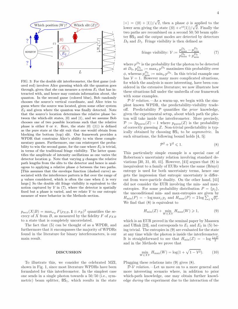
FIG. 3: For the double slit interferometer, the first game (col-ored red) involves Alice guessing which slit the quanton goesthrough, given that she can measure a system E1 that has in-teracted with, and hence may contain information about, thequanton. In the second game (colored blue), Bob randomlychooses the source’s vertical coordinate, and Alice tries toguess where the source was located, given some other systemE2 and given where the quanton was finally detected. Notethat the source’s location determines the relative phase be-tween the which-slit states, |0〉 and |1〉, and we assume Bobchooses one of two possible locations such that the relativephase is either 0 or π. Here, the state |0〉 (|1〉) is definedas the pure state at the slit exit that one would obtain fromblocking the bottom (top) slit. Our framework provides aWPDR that constrains Alice’s ability to win these comple-mentary games. Furthermore, one can reinterpret the proba-bility to win the second game, for the case where E2 is trivial,in terms of the traditional fringe visibility. The latter quan-tifies the amplitude of intensity oscillations as one varies thedetector location y. Note that varying y changes the relativepath lengths from the slits to the detector and hence is anal-ogous to applying a relative phase φ between the two paths.[This assumes that the envelope function (dashed curve) as-sociated with the interference pattern is flat over the range ofy values considered, which is often the case when L is verylarge.] So the double slit fringe visibility is equivalent to thenotion captured by V in (7), where the detector is spatiallyfixed but a phase is varied, and we relate V to our entropicmeasure of wave behavior in the Methods section.

psecr(X |B) = maxσBF (ρXB , 11 ⊗ σB)

2 quantifies the se-crecy of X from B, as measured by the fidelity F of ρXBto a state that is completely uncorrelated.

The fact that (5) can be thought of as a WPDR, andfurthermore that it encompasses the majority of WPDRsfound in the literature for binary interferometers, is ourmain result.

DISCUSSION

To illustrate this, we consider the celebrated MZI,shown in Fig. 1, since most literature WPDRs have beenformulated for this interferometer. In the simplest caseone sends in a single photon towards a 50/50 (i.e., sym-metric) beam splitter, BS1, which results in the state

|+〉 = (|0〉 + |1〉)/√2, then a phase φ is applied to the

lower arm giving the state (|0〉+ eiφ|1〉)/√2. Finally the

two paths are recombined on a second 50/50 beam split-ter BS2 and the output modes are detected by detectorsD0 and D1. Fringe visibility is then defined as

fringe visibility: V :=pD0max − pD0

min

pD0max + pD0

min

, (7)

where pD0 is the probability for the photon to be detectedat D0, p

D0max := maxφ p

D0 maximizes this probability over

φ, whereas pD0

min := minφ pD0 . In this trivial example one

has V = 1. However many more complicated situations,for which the analysis is more interesting, have been con-sidered in the extensive literature; we now illustrate howthese situations fall under the umbrella of our frameworkwith some examples.P-V relation.—As a warm-up, we begin with the sim-

plest known WPDR, the predictability-visibility trade-off. Predictability P quantifies the prior knowledge,given the experimental setup, about which path the pho-ton will take inside the interferometer. More precisely,P := 2pguess(Z) − 1 where pguess(Z) is the probabilityof correctly guessing Z. Non-trivial predictability is typ-ically obtained by choosing BS1 to be asymmetric. Insuch situations, the following bound holds [4, 5]:

P2 + V26 1. (8)

This particularly simple example is a special case ofRobertson’s uncertainty relation involving standard de-viations [30, 31, 40, 41]. However, [41] argues that (8) isinequivalent to a family of EURs where the same (Rényi)entropy is used for both uncertainty terms, hence onegets the impression that entropic uncertainty is differ-ent from wave-particle duality. On the other hand, [41]did not consider the EUR involving the min- and max-entropies. For some probability distribution P = pj,the unconditional min- and max-entropies are given byHmin(P ) = − logmaxj pj and Hmax(P ) = 2 log

∑j

√pj .

We find that (8) is equivalent to

Hmin(Z) + minW∈XY

Hmax(W ) > 1, (9)

which is an EUR proved in the seminal paper by Maassenand Uffink [23], and corresponds to E1 and E2 in (5) be-ing trivial. The entropies in (9) are evaluated for the stateat any time while the photon is inside the interferometer.It is straightforward to see that Hmin(Z) = − log 1+P

2and in the Methods we prove that

minW∈XY

Hmax(W ) = log(1 +√1− V2). (10)

Plugging these relations into (9) gives (8).D-V relation.—Let us move on to a more general and

more interesting scenario where, in addition to priorwhich-path knowledge, one may obtain further knowl-edge during the experiment due to the interaction of the

5

BS1

BS2

removed(A) Prediction

Which willclick?

F

BS1

blocker

BS2

(B) Retrodiction

Which wasblocked?

F

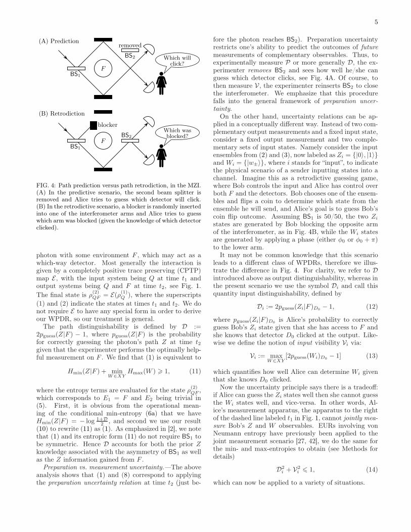
FIG. 4: Path prediction versus path retrodiction, in the MZI.(A) In the predictive scenario, the second beam splitter isremoved and Alice tries to guess which detector will click.(B) In the retrodictive scenario, a blocker is randomly insertedinto one of the interferometer arms and Alice tries to guesswhich arm was blocked (given the knowledge of which detectorclicked).

photon with some environment F , which may act as awhich-way detector. Most generally the interaction isgiven by a completely positive trace preserving (CPTP)map E , with the input system being Q at time t1 andoutput systems being Q and F at time t2, see Fig. 1.

The final state is ρ(2)QF = E(ρ(1)Q ), where the superscripts

(1) and (2) indicate the states at times t1 and t2. We donot require E to have any special form in order to deriveour WPDR, so our treatment is general.

The path distinguishability is defined by D :=2pguess(Z|F ) − 1, where pguess(Z|F ) is the probabilityfor correctly guessing the photon’s path Z at time t2given that the experimenter performs the optimally help-ful measurement on F . We find that (1) is equivalent to

Hmin(Z|F ) + minW∈XY

Hmax(W ) > 1, (11)

where the entropy terms are evaluated for the state ρ(2)QF ,

which corresponds to E1 = F and E2 being trivial in(5). First, it is obvious from the operational mean-ing of the conditional min-entropy (6a) that we haveHmin(Z|F ) = − log 1+D

2 , and second we use our result(10) to rewrite (11) as (1). As emphasized in [2], we notethat (1) and its entropic form (11) do not require BS1 tobe symmetric. Hence D accounts for both the prior Zknowledge associated with the asymmetry of BS1 as wellas the Z information gained from F .

Preparation vs. measurement uncertainty.—The aboveanalysis shows that (1) and (8) correspond to applyingthe preparation uncertainty relation at time t2 (just be-

fore the photon reaches BS2). Preparation uncertaintyrestricts one’s ability to predict the outcomes of future

measurements of complementary observables. Thus, toexperimentally measure P or more generally D, the ex-perimenter removes BS2 and sees how well he/she canguess which detector clicks, see Fig. 4A. Of course, tothen measure V , the experimenter reinserts BS2 to closethe interferometer. We emphasize that this procedurefalls into the general framework of preparation uncer-

tainty.On the other hand, uncertainty relations can be ap-

plied in a conceptually different way. Instead of two com-plementary output measurements and a fixed input state,consider a fixed output measurement and two comple-mentary sets of input states. Namely consider the inputensembles from (2) and (3), now labeled as Zi = |0〉, |1〉and Wi = |w±〉, where i stands for “input”, to indicatethe physical scenario of a sender inputting states into achannel. Imagine this as a retrodictive guessing game,where Bob controls the input and Alice has control overboth F and the detectors. Bob chooses one of the ensem-bles and flips a coin to determine which state from theensemble he will send, and Alice’s goal is to guess Bob’scoin flip outcome. Assuming BS1 is 50/50, the two Zistates are generated by Bob blocking the opposite armof the interferometer, as in Fig. 4B, while the Wi statesare generated by applying a phase (either φ0 or φ0 + π)to the lower arm.

It may not be common knowledge that this scenarioleads to a different class of WPDRs, therefore we illus-trate the difference in Fig. 4. For clarity, we refer to Dintroduced above as output distinguishability, whereas inthe present scenario we use the symbol Di and call thisquantity input distinguishability, defined by

Di := 2pguess(Zi|F )D0 − 1, (12)

where pguess(Zi|F )D0 is Alice’s probability to correctlyguess Bob’s Zi state given that she has access to F andshe knows that detector D0 clicked at the output. Like-wise we define the notion of input visibility Vi via:

Vi := maxW∈XY

[2pguess(Wi)D0 − 1] (13)

which quantifies how well Alice can determine Wi giventhat she knows D0 clicked.

Now the uncertainty principle says there is a tradeoff:if Alice can guess the Zi states well then she cannot guessthe Wi states well, and vice-versa. In other words, Al-ice’s measurement apparatus, the apparatus to the rightof the dashed line labeled t1 in Fig. 1, cannot jointly mea-

sure Bob’s Z and W observables. EURs involving vonNeumann entropy have previously been applied to thejoint measurement scenario [27, 42], we do the same forthe min- and max-entropies to obtain (see Methods fordetails)

D2i + V2

i 6 1, (14)

which can now be applied to a variety of situations.

6

P

|0〉Q

|1〉QBS

F QBS

PBS

PBS

D0,P+

D0,P−

D1,P−

D1,P+

QBS =

ρ(2)P

ρ(2)Q

UPQ

U(R)

FIG. 5: In the quantum beam splitter (QBS) scenario, thesecond beam splitter is in a superposition of “absent” and

“present”, as determined by the polarization state ρ(2)P at

time t2. The QBS can be modelled as a controlled-unitary,UPQ = |H〉〈H |P ⊗ 11Q + |V 〉〈V |P ⊗ U(R), where U(R) is theunitary on Q associated with an asymmetric beam splitterwith reflection probability R. Polarization-resolving detec-tors (PBS = polarizing beam splitter) on the output modeshelp to reveal the “quantumness” of the QBS.

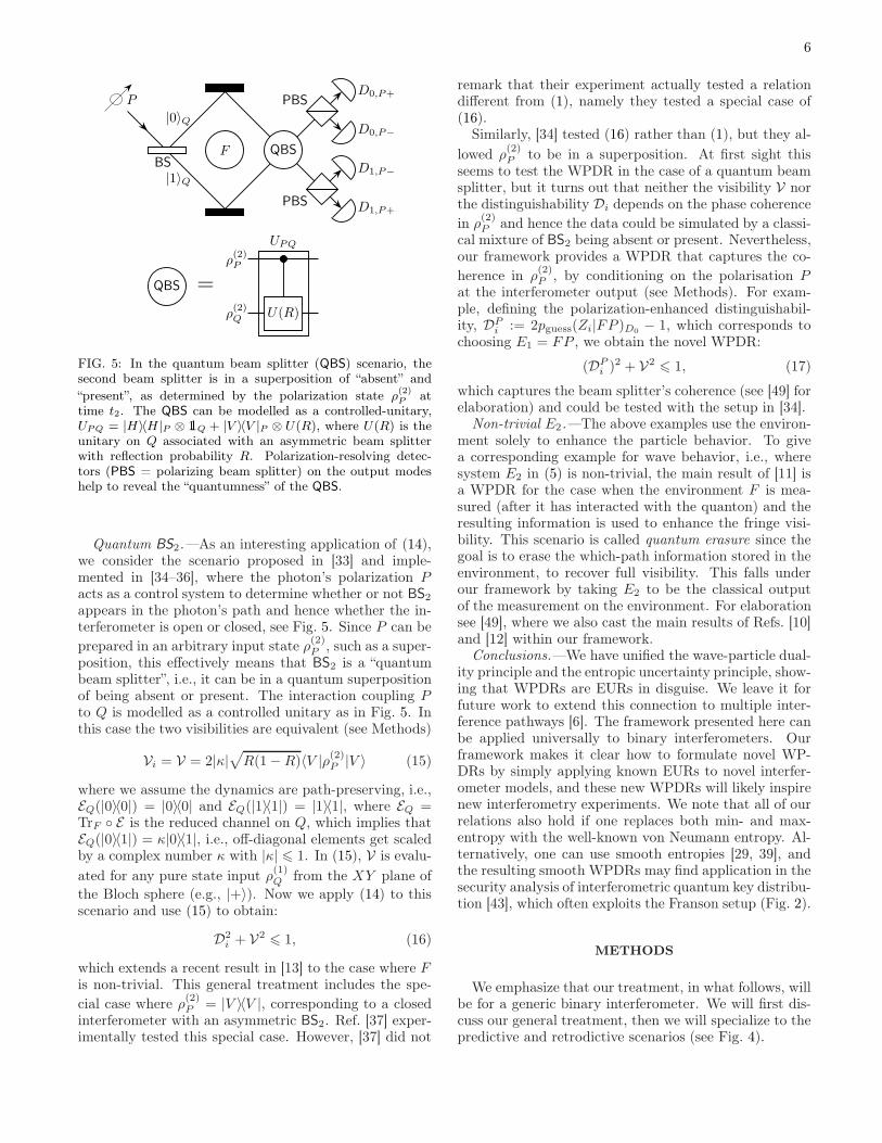
Quantum BS2.—As an interesting application of (14),we consider the scenario proposed in [33] and imple-mented in [34–36], where the photon’s polarization Pacts as a control system to determine whether or not BS2

appears in the photon’s path and hence whether the in-terferometer is open or closed, see Fig. 5. Since P can be

prepared in an arbitrary input state ρ(2)P , such as a super-

position, this effectively means that BS2 is a “quantumbeam splitter”, i.e., it can be in a quantum superpositionof being absent or present. The interaction coupling Pto Q is modelled as a controlled unitary as in Fig. 5. Inthis case the two visibilities are equivalent (see Methods)

Vi = V = 2|κ|√R(1−R)〈V |ρ(2)P |V 〉 (15)

where we assume the dynamics are path-preserving, i.e.,EQ(|0〉〈0|) = |0〉〈0| and EQ(|1〉〈1|) = |1〉〈1|, where EQ =TrF E is the reduced channel on Q, which implies thatEQ(|0〉〈1|) = κ|0〉〈1|, i.e., off-diagonal elements get scaledby a complex number κ with |κ| 6 1. In (15), V is evalu-

ated for any pure state input ρ(1)Q from the XY plane of

the Bloch sphere (e.g., |+〉). Now we apply (14) to thisscenario and use (15) to obtain:

D2i + V2

6 1, (16)

which extends a recent result in [13] to the case where Fis non-trivial. This general treatment includes the spe-

cial case where ρ(2)P = |V 〉〈V |, corresponding to a closed

interferometer with an asymmetric BS2. Ref. [37] exper-imentally tested this special case. However, [37] did not

remark that their experiment actually tested a relationdifferent from (1), namely they tested a special case of(16).

Similarly, [34] tested (16) rather than (1), but they al-

lowed ρ(2)P to be in a superposition. At first sight this

seems to test the WPDR in the case of a quantum beamsplitter, but it turns out that neither the visibility V northe distinguishability Di depends on the phase coherence

in ρ(2)P and hence the data could be simulated by a classi-

cal mixture of BS2 being absent or present. Nevertheless,our framework provides a WPDR that captures the co-

herence in ρ(2)P , by conditioning on the polarisation P

at the interferometer output (see Methods). For exam-ple, defining the polarization-enhanced distinguishabil-ity, DP

i := 2pguess(Zi|FP )D0 − 1, which corresponds tochoosing E1 = FP , we obtain the novel WPDR:

(DPi )

2 + V26 1, (17)

which captures the beam splitter’s coherence (see [49] forelaboration) and could be tested with the setup in [34].

Non-trivial E2.—The above examples use the environ-ment solely to enhance the particle behavior. To givea corresponding example for wave behavior, i.e., wheresystem E2 in (5) is non-trivial, the main result of [11] isa WPDR for the case when the environment F is mea-sured (after it has interacted with the quanton) and theresulting information is used to enhance the fringe visi-bility. This scenario is called quantum erasure since thegoal is to erase the which-path information stored in theenvironment, to recover full visibility. This falls underour framework by taking E2 to be the classical outputof the measurement on the environment. For elaborationsee [49], where we also cast the main results of Refs. [10]and [12] within our framework.

Conclusions.—We have unified the wave-particle dual-ity principle and the entropic uncertainty principle, show-ing that WPDRs are EURs in disguise. We leave it forfuture work to extend this connection to multiple inter-ference pathways [6]. The framework presented here canbe applied universally to binary interferometers. Ourframework makes it clear how to formulate novel WP-DRs by simply applying known EURs to novel interfer-ometer models, and these new WPDRs will likely inspirenew interferometry experiments. We note that all of ourrelations also hold if one replaces both min- and max-entropy with the well-known von Neumann entropy. Al-ternatively, one can use smooth entropies [29, 39], andthe resulting smooth WPDRs may find application in thesecurity analysis of interferometric quantum key distribu-tion [43], which often exploits the Franson setup (Fig. 2).

METHODS

We emphasize that our treatment, in what follows, willbe for a generic binary interferometer. We will first dis-cuss our general treatment, then we will specialize to thepredictive and retrodictive scenarios (see Fig. 4).

7

Origin of general WPDR.—It is known that the min-and max-entropies satisfy the uncertainty relation [29]:

Hmin(Z|E1) +Hmax(W |E2) > 1, (18)

for any tripartite state ρAE1E2 where A is a qubit and Zand W are mutually unbiased bases on A. Noting thatthe which-path and which-path observables in (2) and(3) are mutually unbiased (for all φ0 in (3), i.e., for allW in the XY plane) gives our general WPDR in (5).

Complementary guessing game.—The operational in-terpretation of (5) in terms of the complementary guess-ing game described, e.g., in Figs. 1-3 can be seen clearlyas follows. While the min-entropy is related to the guess-ing probability via (6a), we establish a similar relation forthe max-entropy. First we prove [49] that, for a general

classical-quantum state ρXB =∑

j |j〉〈j| ⊗ σjB where Xis binary,

Hmax(X |B) = log(1 + 2

∣∣∣∣√σ0B

√σ1B

∣∣∣∣1

), (19)

where the 1-norm is ‖M‖1 = Tr√M †M . Next we show

[49], for any positive semi-definite operators M and N ,

||M −N ||21 + 4||√M

√N ||21 6 (TrM +TrN)2. (20)

Combining (20) with (19), and using the well-known for-mula ||σ0

B − σ1B||1 = 2pguess(X |B)− 1, gives

Hmax(X |B) 6 log(1 +

√1− (2pguess(X |B)− 1)2

).

(21)Now one can define generic measures of particle and wavebehavior directly in terms of the guessing probabilities:

Dg := 2pguess(Z|E1)− 1, (22)

Vg := maxW∈XY

[2pguess(W |E2)− 1] (23)

for some arbitrary quantum systems E1 and E2, and re-arrange (5) into the traditional form for WPDRs:

D2g + V2

g 6 1. (24)

This operationally-motivated relation, which follows di-rectly from (5), clearly imposes a restriction on Alice’sability to win the complementary guessing game, sinceDg and Vg are defined in terms of the winning probabili-ties. Below we show that Vg becomes the fringe visibilitywhen E2 is discarded.

Predictive WPDRs.—We now elaborate on our frame-work for deriving predictive WPDRs. Let us denote thequanton’s spatial degree of freedom as S, which includesthe previously mentioned Q as a subspace. At time t2(see, e.g., Fig. 1) - the time just before a phase φ is ap-plied and the interferometer is closed - S and its environ-

ment E are in some state ρ(2)SE , where again E = E1E2 is

a generic bipartite system. The preparation is arbitrary,i.e., we need not specify what happened at earlier times,such as what the system’s state was at time t1 (prior

to the interaction between S and E). While in generala binary interferometer may have more than two paths,all but two of these are non-interfering (by definition),hence we only consider the two-dimensional subspace as-sociated with the two which-path states of interest, de-noted |0〉 and |1〉. This subspace, defined by the projectorΠ := |0〉〈0|+ |1〉〈1|, can be thought of as an effective qubitsystem Q. (Note that Q = S in the MZI.) Without loss

of generality, we project the state ρ(2)SE onto this subspace

and denote the resulting (renormalized) state as

ρ(2)QE = (Π⊗ 11)ρ

(2)SE(Π⊗ 11)/Tr(Πρ

(2)S ). (25)

Experimentally this corresponds to post-selecting on theinterfering portion of the data. To derive predictive WP-

DRs, we apply (5) to the state ρ(2)QE in (25), where we

associate the subsystems E1 and E2 of E with the parti-cle and wave terms respectively.

For example this approach gives the WPDRs discussedin [2], Eqs. (1) and (8). To show this we must prove (10),which relates our entropic measure of wave behavior in(4b) to fringe visibility, and we now do this for genericbinary interferometers. We remark that one can take(7) as a generic definition for fringe visibility, where thelabelD0 is arbitrary, i.e., it corresponds to some arbitrarydetector. For generic binary interferometers, there is aphase shift φ applied just after time t2, as depicted inFig. 1. Let Uφ = |0〉〈0| + eiφ|1〉〈1| denote the unitaryassociated with this phase shift, and note that we onlyneed to specify the action of Uφ on the Q subspace since

the state ρ(2)QE lives in this subspace.

Finally the quanton is detected somewhere, i.e., sys-tem S is measured and a detector D0 clicks. This mea-surement is a positive operator valued measure (POVM)C = C0, C1, ... on the larger space, system S ratherthan the subspace Q (e.g., think of the double slit case,where the detection screen performs a position measure-ment on S). We associate the POVM element C0 with theevent of detector D0 clicking. To prove (10), we need torestrict the form of C0. We show that (10) holds so longas C0 is unbiased with respect to the which-path basis Zon the subspace Q. Fortunately this condition is satisfiedfor all three types of interferometers in Figs. 1, 2, and 3.More precisely, it is satisfied for the MZI provided BS2

is 50/50, for the Franson case provided both BS2 (thesecond beam splitters in Fig. 2) are 50/50, and for thedouble slit for some limiting choice of experimental pa-rameters such as large L in Fig. 3. We now state a generallemma that applies to all of these interferometers.Lemma 1. Consider a binary interferometer whereC0 := ΠC0Π denotes the projection of POVM elementC0 onto the interfering subspace (Q). Suppose C0 is pro-portional to a projector projecting onto a state from theXY plane of the Bloch sphere of Q, i.e.,

C0 = q|w+〉〈w+| (26)

for some 0 < q 6 1, where |w+〉 is given by (3) for some

8

arbitrary phase φ0. Then it follows that

minW∈XY

Hmax(W ) = log(1 +√1− V2), (27)

where V is given by (7), and Hmax(W ) is evaluated for

the state ρ(2)Q = TrE(ρ

(2)QE).

Proof. In what follows it should be understood that prob-abilities and expectation values are evaluated for the

state ρ(2)Q . Suppose that W is optimal in the sense

that maxW∈XY Pr(w+) = Pr(w+) where Pr(w±) :=

〈w±|ρ(2)Q |w±〉. Then we have

minW∈XY

Hmax(W ) = log(1 +

√1− 〈σ

W〉2)

(28)

where we denote Pauli operators by σW := |w+〉〈w+| −|w−〉〈w−|, and 〈σ

W〉 = Pr(w+)− Pr(w−).

The probability for D0 to click is

pD0 = Tr(C0Uφρ(2)Q U †

φ) = Tr(U †φC0Uφρ

(2)Q ) (29)

and maximising this over φ gives

pD0max = q max

W∈XYPr(w+) = q Pr(w+). (30)

Now, due to the geometry of the Bloch sphere, we havepD0

min = Pr(w−). Thus, pD0max+p

D0

min = q and pD0max−pD0

min =q〈σ

W〉. This gives V = 〈σ

W〉, completing the proof.

Retrodictive WPDRs.—While we saw that the predic-tive approach allowed for any preparation but requiredcomplementary output measurements, the opposite istrue in the retrodictive case, i.e., the form of the outputmeasurement is arbitrary while we require complemen-tary preparations. The input ensembles Zi = |0〉, |1〉and Wi = |w+〉, |w−〉 can be generated by performingthe relevant measurements on a reference qubit Q′ thatis initially entangled to the quanton S. Associating stateensembles with measurements on a reference system is auseful trick, e.g., for deriving (14). Thus, at time t1 (justafter the quanton enters the interferometer, see Fig. 1)we introduce a qubit Q′ that is maximally entangled tothe interfering subspace (Q) of S, denoted by the state

ρ(1)Q′S = |Φ〉〈Φ| with |Φ〉 = (|00〉+|11〉)/

√2. The dynamics

after time t1 is modelled as a quantum operation A, de-fined in [44] as a completely positive, trace non-increasingmap, that maps S → E1E2. The output of A does notcontain S because the quanton is eventually detected bya detector, at which point we no longer need a quantumdescription the quanton’s spatial degree of freedom; weonly care where it was detected. The map A correspondsto a particular detection event; for concreteness say thatdetector D0 clicking is the associated event. The prob-ability for this event is the trace of the state after theaction of A, and renormalizing gives the final state

ρD0

Q′E1E2:=

(I ⊗ A)(ρ(1)Q′S)

Tr[(I ⊗ A)(ρ(1)Q′S)]

. (31)

Our framework applies the uncertainty relation (5) to the

state ρD0

Q′E1E2to derive retrodictive WPDRs.

For example, this covers the scenario from the Discus-sion where A involves two sequential steps. First S in-teracts with an environment F inside the interferometerbetween times t1 and t2, which corresponds to a channelE mapping S to SF . Second, the quanton is detectedat the interferometer output, say at detector D0, mod-elled as a map B(·) = TrS [C0(·)] acting on S, where C0 isthe POVM element associated with detector D0 clicking.Hence we choose A = B E . Applying (5) to this casewhile choosing E1 = F and E2 to be trivial gives

Hmin(Z|F )ρ + minW∈XY

Hmax(W )ρ > 1, (32)

where the subscript ρ means evaluating on the state in(31). Note that measuring Z on system Q′ correspondsto sending the states |0〉, |1〉 with equal probabilitythrough the interferometer, and similarly for W (with aninconsequential complication of taking the transpose ofthe W basis states). Realizing this, the first and secondterms in (32) map onto Di and Vi respectively:

Hmin(Z|F )ρ = 1− log(1 +Di), (33)

minW∈XY

Hmax(W )ρ = log(1 +√1− V2

i ). (34)

Hence (32) becomes (14).It remains to show that Vi appearing in (14) can be

replaced by V for many cases of interest, such as the QBS

case. We do this in the following lemma, where the proofis given in [49] and is similar to the proof of Lemma 1.Lemma 2. Consider any binary interferometer with anunbiased input, i.e., where the state at time t1 is unbi-ased with respect to the which-path basis (of the form

|ψ(1)Q 〉 = (|0〉 + eiφ|1〉)/

√2). Let ES = TrF E be the

channel describing the quanton’s interaction with F in-side the interferometer, and let G(·) = Π(·)Π be the mapthat projects onto the subspace Π. Suppose ES is path-preserving, i.e., ES(|0〉〈0|) = |0〉〈0| and ES(|1〉〈1|) = |1〉〈1|and furthermore suppose ES commutes with G. Then

minW∈XY

Hmax(W )ρ = log(1 +√1− V2), (35)

where Hmax(W ) is evaluated for the state ρD0

Q′ .QBS example.—Finally, we treat the quantum beam

splitter shown in Fig. 5. (Note that S = Q in the MZI.)This setup involves first a quantum channel E that de-scribes the interaction of S with an environment F be-tween times t1 and t2, followed by another channel as-sociated with the QBS that interacts S with the polar-ization P , followed by a post-selected detection at D0.Together these three steps form a quantum operation Athat maps S → FP , and hence this falls under our retro-dictive framework.

To prove (17) we apply (5) to the state in (31) whilechoosing E1 = FP and E2 to be trivial, giving

Hmin(Z|FP )ρ + minW∈XY

Hmax(W )ρ > 1. (36)

9

We then use relations analogous to those in (33) and (34),where the former relation now involves conditioning alsoon the polarisation P . Finally, we note that Lemma 2applies to the QBS case.

ACKNOWLEDGEMENTS

We thank B. Englert and S. Tanzilli for helpful corre-spondence, and acknowledge helpful discussions with M.

Woods, M. Tomamichel, C. J. Kwong, and L. C. Kwek.We acknowledge funding from the Ministry of Education(MOE) and National Research Foundation Singapore, aswell as MOE Tier 3 Grant “Random numbers from quan-tum processes” (MOE2012-T3-1-009).

[1] R. P. Feynman, Feynman Lectures on Physics (AddisonWesley, Longman, 1970).

[2] B.-G. Englert, Phys. Rev. Lett. 77, 2154 (1996).[3] G. Jaeger, A. Shimony, and L. Vaidman, Phys. Rev. A

51, 54 (1995).[4] W. K. Wootters and W. H. Zurek, Phys. Rev. D 19, 473

(1979).[5] D. M. Greenberger and A. Yasin, Physics Letters A 128,

391 (1988), ISSN 0375-9601.[6] B.-G. Englert, D. Kaszlikowski, L. C. Kwek, and W. H.

Chee, International Journal of Quantum Information 06,129 (2008).

[7] N.-L. Liu, L. Li, S. Yu, and Z.-B. Chen, Phys. Rev. A79, 052108 (2009).

[8] J.-H. Huang, S. Wölk, S.-Y. Zhu, and M. S. Zubairy,Phys. Rev. A 87, 022107 (2013).

[9] T. Qureshi, Progress of Theoretical and ExperimentalPhysics 2013 (2013).

[10] L. Li, N.-L. Liu, and S. Yu, Phys. Rev. A 85, 054101(2012).

[11] B.-G. Englert and J. A. Bergou, Optics Communications179, 337 (2000), ISSN 0030-4018.

[12] K. Banaszek, P. Horodecki, M. Karpiński, andC. Radzewicz, Nat Commun 4 (2013).

[13] A.-A. Jia, J.-H. Huang, W. Feng, T.-C. Zhang, and S.-Y.Zhu, Chinese Physics B 23, 30307 (2014).

[14] B.-G. Englert, M. O. Scully, and H. Walther, Nature 375,367 (1995).

[15] P. Storey, S. Tan, M. Collett, and D. Walls, Nature 367,626 (1994).

[16] H. Wiseman and F. Harrison, Nature 377, 584 (1995).[17] N. Bohr, Nature 121, 580 (1928).[18] W. Heisenberg, Zeitschrift für Physik 43, 172 (1927).[19] E. Kennard, Z. Phys 44, 326 (1927).[20] H. P. Robertson, Phys. Rev. 34, 163 (1929).[21] D. Deutsch, Physical Review Letters 50, 631 (1983).[22] I. Białynicki-Birula and J. Mycielski, Communications in

Mathematical Physics 44, 129 (1975).[23] H. Maassen and J. B. M. Uffink, Phys. Rev. Lett. 60,

1103 (1988).[24] S. Wehner and A. Winter, New J. Phys. 12, 025009

(2010).[25] J. M. Renes and J.-C. Boileau, Phys. Rev. Lett. 103,

020402 (2009).[26] M. Berta, M. Christandl, R. Colbeck, J. M. Renes, and

R. Renner, Nature Physics 6, 659 (2010).[27] P. J. Coles, L. Yu, V. Gheorghiu, and R. B. Griffiths,

Phys. Rev. A 83, 062338 (2011).

[28] P. J. Coles, R. Colbeck, L. Yu, and M. Zwolak, Phys.Rev. Lett. 108, 210405 (2012).

[29] M. Tomamichel and R. Renner, Phys. Rev. Lett. 106,110506 (2011).

[30] S. Durr and G. Rempe, American Journal of Physics 68,1021 (2000).

[31] P. Busch and C. Shilladay, Physics Reports 435, 1(2006), ISSN 0370-1573.

[32] R. Konig, R. Renner, and C. Schaffner, IEEE Trans. Inf.Theory 55, 4337 (2009).

[33] R. Ionicioiu and D. R. Terno, Phys. Rev. Lett. 107,230406 (2011).

[34] F. Kaiser, T. Coudreau, P. Milman, D. B. Ostrowsky,and S. Tanzilli, Science 338, 637 (2012).

[35] A. Peruzzo, P. Shadbolt, N. Brunner, S. Popescu, andJ. L. O’Brien, Science 338, 634 (2012).

[36] J.-S. Tang, Y.-L. Li, C.-F. Li, and G.-C. Guo, Phys. Rev.A 88, 014103 (2013).

[37] V. Jacques, E. Wu, F. Grosshans, F. Treussart, P. Grang-ier, A. Aspect, and J.-F. Roch, Phys. Rev. Lett. 100,220402 (2008).

[38] J. D. Franson, Phys. Rev. Lett. 62, 2205 (1989).[39] M. Tomamichel, C. C. W. Lim, N. Gisin, and R. Renner,

Nature Communications 3, 634 (2012).[40] G. Björk, J. Söderholm, A. Trifonov, T. Tsegaye, and

A. Karlsson, Phys. Rev. A 60, 1874 (1999).[41] G. M. Bosyk, M. Portesi, F. Holik, and A. Plastino, Phys-

ica Scripta 87, 065002 (2013).[42] F. Buscemi, M. J. W. Hall, M. Ozawa, and M. M. Wilde,

Phys. Rev. Lett. 112, 050401 (2014).[43] A. K. Ekert, J. G. Rarity, P. R. Tapster, and G. Mas-

simo Palma, Phys. Rev. Lett. 69, 1293 (1992).[44] M. A. Nielsen and I. L. Chuang, Quantum Computation

and Quantum Information (Cambridge University Press,Cambridge, 2000), 5th ed.

[45] C. W. Helstrom, Quantum detection and estimation the-ory (Academic Press, New York, USA, 1976), ISBN0123400503.

[46] C. King and M. Ruskai, IEEE Trans. Inf. Theory 47, 192(2001).

[47] S. Tanzilli, private communication.[48] U. Herzog and J. A. Bergou, Phys. Rev. A 70, 022302

(2004).[49] See the Supplementary Information.

10

Supplementary Information

Contents

I. Introduction 10

II. Relating max-entropy to guessing probability 10

III. Hybrid of predictive and retrodictive scenarios 13A. Introduction 13B. General treatment of hybrid scenario 13C. Proof of Lemma S7 (generalized version of Lemma 2) 16

IV. Enhanced visibility 17A. Quantum erasure 18

1. Results of Ref. [11] 182. Our treatment 18

B. Polarization-enhanced visibility and discussion of Ref. [12] 191. Result of Ref. [12] 192. Our treatment 203. Proof of Lemma S9 21

V. Testing coherence in a quantum beam splitter 22A. Quantities sensitive to coherence 22B. Discussion of Ref. [34] 23C. Derivation of distinguishability formulas 25D. Measuring DP

i 25

I. INTRODUCTION

In this Supplementary Information, we elaborate on the technical details justifying our claims. Furthermore, toemphasize the universality of our framework, we provide additional results showing that other WPDRs appearing inthe literature can be phrased within our framework.

In what follows, Sec. II proves the relation between the max-entropy and the guessing probability given in theMethods section. In Sec. III we extend our framework to scenarios where both the preparation (at the interferometerinput) and the measurement outcome (at the interferometer output) may provide information about the quanton’spath (inside the interferometer). Such situations are a “hybrid” of the predictive and retrodictive scenarios discussedin the main text. This extension allows us to reinterpret a result in Ref. [10] for asymmetric beam splitters as anentropic uncertainty relation and hence show that it falls under our framework. Subsection III C proves Lemma 2from the main text, or in fact, proves a generalized version of this lemma that holds for these “hybrid” scenarios.In Sec. IV we consider WPDRs involving enhanced visibilty. In particular we show that the results of Ref. [11] forquantum erasure and Ref. [12] for polarization dynamics can both be viewed as entropic uncertainty relations, wherethe visibility term is enhanced by conditioning on additional information. Finally in Sec. V we elaborate on our novelWPDR for the quantum beam splitter, demonstrating that it captures the coherence in the QBS and discussing howthe polarization-enhanced distinguishability can be measured.

II. RELATING MAX-ENTROPY TO GUESSING PROBABILITY

Here we relate the max-entropy to the guessing probability. The main lemma that we prove explicitly solves for themax-entropy of a classical-quantum (cq) state where the classical register is binary, which to our knowledge is a newresult. An arbitrary cq state where the classical register is binary, which is the only case relevant to our analysis, canbe written as ρXB = |0〉〈0 |⊗σ0+ |1〉〈1 |⊗σ1, where σ0 and σ1 are subnormalized states that satisfy Trσ0+Trσ1 = 1.In this case, the optimal guessing probability takes the form

pguess(X |B) := maxM0,M1

Tr(M0σ0) + Tr(M1σ1), (S37)

11

where the maximization is taken over all POVMs on subsystem B, namely operators M0,M1 > 0 such that M0 +M1 = 11. Since this is exactly the state discrimination problem solved by Helstrom [45] we have

pguess(X |B) =1

2+

1

2||σ0 − σ1||1. (S38)

Hence the guessing probability is related to the trace distance between the conditional states.The formula for the max-entropy was given in Eq. (6b) from the main text and was expressed in terms of the

fidelity, which is defined as

F (M,N) :=∣∣∣∣√M

√N∣∣∣∣1, (S39)

for two positive semi-definite operators M and N . In our case of a cq state with a binary register, the formula givenin Eq. (6b) simplifies to [32]

Hmax(X |B) = 2 logmaxρ

(F (σ0, ρ) + F (σ1, ρ)

), (S40)

where the maximization is taken over all normalized states on B. The following lemma derives the optimal value ofthis optimization problem.Lemma S3. Let M,N > 0 be positive semi-definite operators and let S be the set of positive semi-definite operatorswith unit trace. Then

maxρ∈S

(F (M,ρ) + F (N, ρ)

)=

√TrM +TrN + 2F (M,N). (S41)

Proof. First, we show that the right-hand side constitutes a valid upper bound and then we give an explicit choice ofρ that achieves it.

For arbitrary unitaries U0 and U1 let X† = U0

√M + U1

√N and Y =

√ρ. The Cauchy-Schwarz inequality,

|Tr(X†Y )|2 6 Tr(X†X) · Tr(Y †Y ), implies that

∣∣∣Tr((U0

√M + U1

√N)√ρ)∣∣∣

2

6 Tr(X†X) · Trρ = Tr(X†X). (S42)

Since

X†X = U0MU †0 + U1NU

†1 + U0

√M

√NU †

1 + U1

√N√MU †

0 (S43)

we have

Tr(X†X) = TrM +TrN +Tr(U0

√M

√NU †

1 + U1

√N√MU †

0

)(S44)

6 TrM +TrN +∣∣∣∣U0

√M

√NU †

1 + U1

√N√MU †

0

∣∣∣∣1

(S45)

6 TrM +TrN + 2∣∣∣∣√M

√N∣∣∣∣1= TrM +TrN + 2F (M,N), (S46)

where we have used the fact that for Hermitian matrices Tr T 6 ||T ||1 followed by the triangle inequality for the1-norm. Note that this bound is valid for all unitaries U0 and U1.

Let L be a linear operator and let L = U0SU1 be its singular value decomposition. Clearly, ||L||1 = Tr(V L) for

V = U †1U

†0 . Therefore, for every pair of positive semi-definite operators A and B there exists a unitary V such that

F (A,B) = ||√A√B||1 = Tr(V

√A√B). Let us choose unitaries V0 and V1 such that

F (M,ρ) = Tr(V0

√M

√ρ)

and F (N, ρ) = Tr(V1

√N√ρ). (S47)

Adding these two terms together gives

F (M,ρ) + F (N, ρ) = Tr(V0

√M

√ρ)+Tr

(V1

√N√ρ)= Tr

((V0

√M + V1

√N)√ρ). (S48)

Since for this particular choice of unitaries the quantity on the right-hand side is real and positive we can apply (S42)to obtain

F (M,ρ) + F (N, ρ) =∣∣∣Tr

((V0

√M + V1

√N)√ρ)∣∣∣ 6

√TrM +TrN + 2F (M,N). (S49)

12

Now, we simply need to provide a state ρ that saturates this inequality. Taking advantage of the singular value de-composition of

√M

√N = U0SU1 (where S is a diagonal matrix of real, non-negative numbers and TrS = ||

√M

√N ||1)

we define V = U †1U

†0 and

K =M +N +√MV †√N +

√NV

√M. (S50)

Note that K > 0 since K = L†L for L =√M + V †√N . It is easy to verify that

Tr(√MV †√N

)= Tr

(√NV

√M

)= TrS = ||

√M

√N ||1 = F (M,N), (S51)

which implies that

TrK = TrM +TrN + 2F (M,N) (S52)

To calculate F (M,K) = ||√M

√K||1 = Tr

√√MK

√M note that

√MK

√M =M2 +

√MN

√M +MV †√N

√M +

√M

√NVM (S53)

=M2 + U0S2U †

0 +MU0SU†0 + U0SU

†0M (S54)

=(M + U0SU

†0

)2. (S55)

Therefore, F (M,K) = TrM + F (M,N) and similarly F (N,K) = TrN + F (M,N). Since

F (αA,B) = ||√αA

√B||1 =

√α||

√A√B||1 =

√αF (A,B) (S56)

we can define ρ = K/TrK which satisfies

F (M,ρ) + F (N, ρ) =F (M,K) + F (N,K)√

TrK=

√TrM +TrN + 2F (M,N) (S57)

and saturates the bound (S49).

Now taking the above lemma and setting M = σ0 and N = σ1 allows us to solve the maximization in (S40). Weobtain the following result.Lemma S4. For any cq state ρXB = |0〉〈0 | ⊗ σ0 + |1〉〈1 | ⊗ σ1 where X is binary,

Hmax(X |B) = log(1 + 2F (σ0, σ1)

). (S58)

Finally we relate the fidelity in (S58) to the trace distance in the guessing probability (S38) with the followinglemma.Lemma S5. Let M,N > 0 be two positive semi-definite operators. Then we have

||M −N ||21 + 4||√M

√N ||21 6 (TrM +TrN)2. (S59)

Proof. Let |Ω〉 = ∑k |k〉|k〉 and consider |ψM 〉 = (

√M ⊗ 11)|Ω〉 and |ψN 〉 = (

√N ⊗ U)|Ω〉, where U is a unitary. It is

easy to verify that

〈ψM |ψN 〉 = 〈Ω |√M

√N ⊗ U |Ω〉 = Tr(

√M

√NUT ), (S60)

where T denotes the transpose in the standard basis. By choosing UT = U †2U

†1 , where U1 and U2 come from the

singular value decomposition of√M

√N = U1SU2 we obtain 〈ψM |ψN 〉 = TrS = ||

√M

√N ||1. Let Tr2 denote partial

trace over the second subsystem. It is easy to check that Tr2|ψM 〉〈ψM | = M and Tr2|ψN 〉〈ψN | = N . Since the tracenorm is non-increasing under the partial trace we have

||M −N ||1 6

∣∣∣∣∣∣|ψM 〉〈ψM | − |ψN 〉〈ψN |

∣∣∣∣∣∣1. (S61)

The rank of the Hermitian matrix H = |ψM 〉〈ψM | − |ψN 〉〈ψN | is at most 2 and let us denote the non-zero eigenvaluesby λ1 and λ2. It is easy to verify that

λ1 + λ2 = TrH = 〈ψM |ψM 〉 − 〈ψN |ψN 〉, (S62)

λ21 + λ22 = TrH2 =(〈ψM |ψM 〉

)2+(〈ψN |ψN 〉

)2 − 2|〈ψM |ψN 〉|2. (S63)

13

Since λ1λ2 = 12

[(λ1 + λ2)

2 − (λ21 + λ22)]= |〈ψM |ψN 〉|2 − 〈ψM |ψM 〉〈ψN |ψN 〉, the Cauchy-Schwarz inequality ensures

that λ1λ2 6 0. As H is Hermitian, we have ||H ||1 = |λ1|+ |λ2| and since the eigenvalues have opposite signs we canwrite it as

||H ||1 = |λ1 − λ2| =√(λ1 − λ2)2. (S64)

Expanding the square gives

(λ1 − λ2)2 = λ21 + λ22 − 2λ1λ2 (S65)

=(〈ψM |ψM 〉

)2+(〈ψN |ψN 〉

)2 − 2|〈ψM |ψN 〉|2 + 2〈ψM |ψM 〉〈ψN |ψN 〉 − 2|〈ψM |ψN 〉|2 (S66)

=(〈ψM |ψM 〉+ 〈ψN |ψN 〉

)2 − 4|〈ψM |ψN 〉|2, (S67)

which combined with (S64) implies

∣∣∣∣∣∣|ψM 〉〈ψM | − |ψN 〉〈ψN |

∣∣∣∣∣∣1=

√(〈ψM |ψM 〉+ 〈ψN |ψN 〉

)2 − 4|〈ψM |ψN 〉|2 (S68)

=

√(TrM +TrN)2 − 4||

√M

√N ||21. (S69)

Combining Lemmas S4 and S5 gives the following result.Lemma S6. For any cq state ρXB where X is binary,

Hmax(X |B) 6 log

(1 +

√1− [2pguess(X |B)− 1]2

). (S70)

Proof. Apply Lemma S5 to the subnormalized states σ0 and σ1 appearing in Lemma S4 to give

‖σ0 − σ1‖21 + 4‖√σ0√σ1‖21 6 1. (S71)

Since ||√σ0√σ1||1 = F (σ0, σ1) combining this inequality with (S58) and (S38) gives the desired inequality.

III. HYBRID OF PREDICTIVE AND RETRODICTIVE SCENARIOS

A. Introduction

In the main text we discussed how to derive WPDRs from preparation and measurement uncertainty relations, whichrespectively deal with predicting the future and retrodicting the past. In this section we show that our frameworkcan also be applied to scenarios that involves a hybrid (or mixture) of prediction and retrodiction.

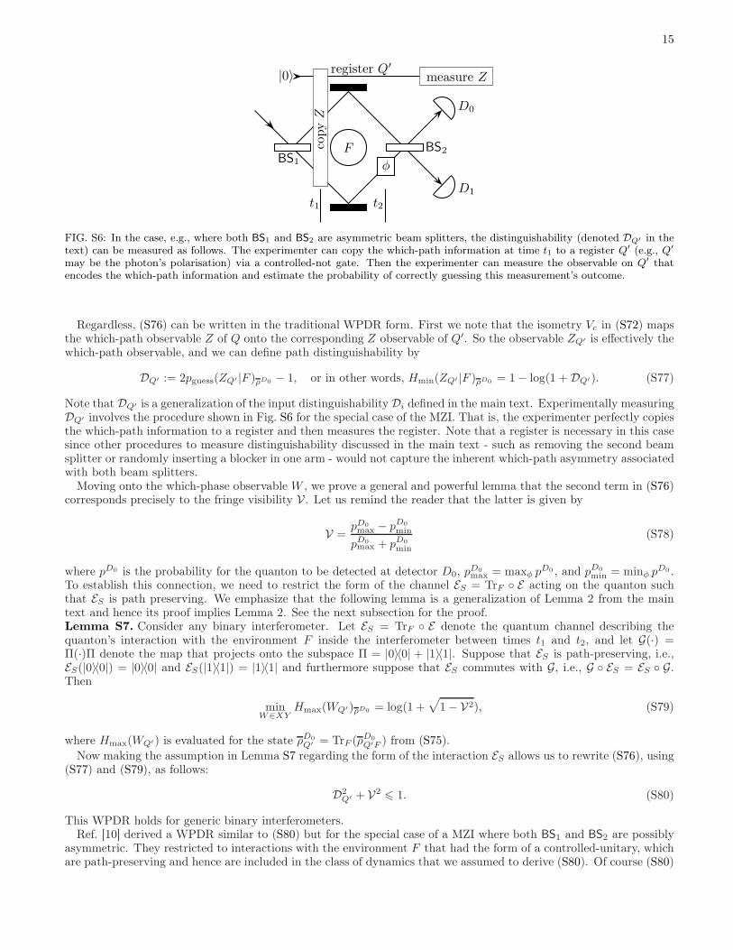
Let us first mention a motivating example from the literature for when this hybrid situation can arise. Ref. [10]considered a simple yet insightful scenario involving a MZI where both beamsplitters BS1 and BS2 (see, e.g., Fig. S6)may be asymmetric. Since BS1 is asymmetric, the experimenter has prior knowledge about which path the photonwill take. Since BS2 is asymmetric, the experimenter can use the final measurement outcome of which detector clickedto help retrodict which path the photon took. Ref. [10] formulated a WPDR for this scenario, and by the end of thissection it will be clear that this falls under our framework. But let us develop the general idea first.

B. General treatment of hybrid scenario

To treat the hybrid case we will consider our retrodictive framework (discussed in the Methods) and add in thepossibility of pre-experiment information about which path the quanton will take. Recall that, in the retrodictivecase, we introduced a qubit register Q′ that is maximally entangled to the quanton S at time t1, the time just afterthe quanton enters the interferometer. More precisely Q′ is maximally entangled to the interfering subspace Q of S.The purpose of Q′ is to store a record of the quanton’s properties at time t1, so that when the quanton evolves andchanges over time, we can still go back to Q′ to ask about the quanton’s properties at the earlier time.

The fact that we chose a maximally entangled state is connected to the fact that there is no prior knowledge aboutthe path the quanton will take. But now we are relaxing that assumption, so we will consider a partially entangled

14

state. It is useful to think of this partially entangled state as arising from taking the physical state ρ(1)S at time t1,

and then applying an isometry Vc that copies the which-path information and stores it in Q′. This isometry expandsthe Hilbert space, mapping S to Q′S as follows:

Vc =

1∑

j=0

|j〉Q′ ⊗ |j〉〈j|S , ρ(1)Q′S := Vcρ

(1)Q V †

c . (S72)

There is a minor technical detail in (S72) that is irrelevant to the MZI but becomes relevant, e.g., in the Franson

interferometer. Namely, in (S72), instead of using the initially-prepared state ρ(1)S , which may have support outside

of the interfering subspace Q, we use the projected and renormalized state ρ(1)Q , defined as

ρ(1)Q := N1 · (Πρ(1)S Π), with N1 := 1/Tr(Πρ

(1)S ), and Π = |0〉〈0|+ |1〉〈1|. (S73)

As discussed in the Methods section, the physical motivation behind this projection is that it corresponds to the

experimenter post-selecting on the interfering portion of the data. Note that if ρ(1)Q is a pure state from the XY plane

of the Bloch sphere (i.e., of the form (|0〉+ eiφ|1〉)/√2), then ρ

(1)Q′S is maximally entangled and then we are just back

to the retrodictive case discussed in the Methods. The generality in the present treatment comes from the fact that

ρ(1)Q is arbitrary.

As in the Methods, we treat the dynamics after time t1 very generally by saying that some quantum operation [44](completely positive trace non-increasing map) denoted A acts on system S, mapping S to the joint system E1E2.The output system does not contain S because the quanton is eventually detected by a detector, at which point we areno longer interested in discussing the quanton’s spatial degree of freedom quantum mechanically; we only care whereit was detected. The map A corresponds to a particular detection event; for concreteness let us say that detector D0

clicking is the associated detection event. The probability for this event is the trace of the state after the action ofA, and upon renormalizing we arrive at the final state

ρD0

Q′E1E2:=

(I ⊗ A)(ρ(1)Q′S)

Tr[(I ⊗ A)(ρ(1)Q′S)]

. (S74)

To derive WPDRs for the hybrid scenario, we apply the our main uncertainty relation, Eq. (5) from the main text,

to the state ρD0

Q′E1E2.

Consider the following important special case, where the map A involves two sequential steps. First there isinteraction between S and an environment F inside the interferometer between times t1 and t2, which corresponds

to feeding S through a channel E , mapping S to SF , obtaining the state ρ(2)Q′SF = (I ⊗ E)(ρ(1)Q′S). Second, system S

is detected at the interferometer output, say at detector D0, which we can model as a map B(·) = TrS [C0(·)], whereC0 is the POVM element (acting on S at time t2) associated with detector D0 clicking. Hence we choose A = B E ,giving the (renormalized) state:

ρD0

Q′F :=TrS(C0ρ

(2)Q′SF )

Tr(C0ρ(2)Q′SF )

. (S75)

Now applying our main uncertainty relation to the state ρD0

Q′F and choosing E2 to be trivial and E1 = F gives

Hmin(ZQ′ |F )ρD0 + minW∈XY

Hmax(WQ′)ρD0 > 1, (S76)

where the subscript ρD0 means evaluating the entropy on the state in (S75) and the subscript Q′ is used to emphasizethat the observables Z and W refer to system Q′.

At this point we must remark on the physical meaning of a relation such as (S76). In the special where the state

ρ(1)Q′S was maximally entangled, as considered in the main text, we noted that (S76) can be interpreted as a joint

measurement relation. This is because a maximally entangled state is special in that it maps observables on registerQ′ to the transpose observables on the system of interest. However this interpretation is lost once we relax the form

of ρ(1)Q′S , so we can no longer interpret (S76) as a joint measurement relation, in the general case. Rather, one can

think of (S76) as a hybrid between a preparation and measurement uncertainty relation.

15

copyZ

measure Zregister Q′

BS1

BS2F

|0〉

t1 t2

φ

D0

D1

FIG. S6: In the case, e.g., where both BS1 and BS2 are asymmetric beam splitters, the distinguishability (denoted DQ′ in thetext) can be measured as follows. The experimenter can copy the which-path information at time t1 to a register Q′ (e.g., Q′

may be the photon’s polarisation) via a controlled-not gate. Then the experimenter can measure the observable on Q′ thatencodes the which-path information and estimate the probability of correctly guessing this measurement’s outcome.

Regardless, (S76) can be written in the traditional WPDR form. First we note that the isometry Vc in (S72) mapsthe which-path observable Z of Q onto the corresponding Z observable of Q′. So the observable ZQ′ is effectively thewhich-path observable, and we can define path distinguishability by

DQ′ := 2pguess(ZQ′ |F )ρD0 − 1, or in other words, Hmin(ZQ′ |F )ρD0 = 1− log(1 +DQ′). (S77)

Note that DQ′ is a generalization of the input distinguishability Di defined in the main text. Experimentally measuringDQ′ involves the procedure shown in Fig. S6 for the special case of the MZI. That is, the experimenter perfectly copiesthe which-path information to a register and then measures the register. Note that a register is necessary in this casesince other procedures to measure distinguishability discussed in the main text - such as removing the second beamsplitter or randomly inserting a blocker in one arm - would not capture the inherent which-path asymmetry associatedwith both beam splitters.

Moving onto the which-phase observable W , we prove a general and powerful lemma that the second term in (S76)corresponds precisely to the fringe visibility V . Let us remind the reader that the latter is given by

V =pD0max − pD0

min

pD0max + pD0

min

(S78)

where pD0 is the probability for the quanton to be detected at detector D0, pD0max = maxφ p

D0 , and pD0

min = minφ pD0 .

To establish this connection, we need to restrict the form of the channel ES = TrF E acting on the quanton suchthat ES is path preserving. We emphasize that the following lemma is a generalization of Lemma 2 from the maintext and hence its proof implies Lemma 2. See the next subsection for the proof.Lemma S7. Consider any binary interferometer. Let ES = TrF E denote the quantum channel describing thequanton’s interaction with the environment F inside the interferometer between times t1 and t2, and let G(·) =Π(·)Π denote the map that projects onto the subspace Π = |0〉〈0| + |1〉〈1|. Suppose that ES is path-preserving, i.e.,ES(|0〉〈0|) = |0〉〈0| and ES(|1〉〈1|) = |1〉〈1| and furthermore suppose that ES commutes with G, i.e., G ES = ES G.Then

minW∈XY

Hmax(WQ′)ρD0 = log(1 +√1− V2), (S79)

where Hmax(WQ′) is evaluated for the state ρD0

Q′ = TrF (ρD0

Q′F ) from (S75).

Now making the assumption in Lemma S7 regarding the form of the interaction ES allows us to rewrite (S76), using(S77) and (S79), as follows:

D2Q′ + V2

6 1. (S80)

This WPDR holds for generic binary interferometers.Ref. [10] derived a WPDR similar to (S80) but for the special case of a MZI where both BS1 and BS2 are possibly

asymmetric. They restricted to interactions with the environment F that had the form of a controlled-unitary, whichare path-preserving and hence are included in the class of dynamics that we assumed to derive (S80). Of course (S80)

16

applies very generally to binary interferometers, but it can be applied to the MZI (note that Q = S in the MZI case)where both BS1 and BS2 are asymmetric. Thus, we find that the result in Ref. [10] can be understood as an entropicuncertainty relation, namely a special case of (S76) [from which we derived (S80)]. To be more precise, Ref. [10] alsogeneralized their relation to allow for non-optimal strategies for measuring F ; we do not treat this generalization here.We believe the most important conceptual advance of Ref. [10] was to prove a WPDR that applies to a scenario that- in our language - is a hybrid of preparation and measurement uncertainty. What we have emphasized in this sectionis that our framework naturally extends to this hybrid scenario.

C. Proof of Lemma S7 (generalized version of Lemma 2)

To prove Lemma S7 we will make use of the following lemma.Lemma S8. Let Q be a qubit quantum channel, i.e., whose input and output are operators on a 2-dimensional Hilbertspace, and suppose that Q(|j〉〈j|) = |j〉〈j| for j = 0, 1. Likewise let Rφ be a qubit quantum channel whose action isgiven by

Rφ(·) = Uφ(·)U †φ, with Uφ = |0〉〈0|+ eiφ|1〉〈1|. (S81)

Then, for any φ, Q and Rφ commute, i.e., Rφ Q = Q Rφ.

Proof. Since Q is unital and furthermore preserves the Z-basis, its action on the Bloch sphere can only involvea rotation Rθ about the Z-axis composed with a shrinking S of the Bloch sphere, and this shrinking must becylindrically symmetric about the Z-axis (see, e.g., Ref. [46]). The rotation Rθ obviously commutes with the rotationRφ, and likewise Rφ commutes with the shrinking S due to the cylindrically symmetry of S.

Now we prove Lemma S7, which relates the fringe visibility to the max-entropy of the which-phase observable inour “hybrid” framework. Lemma S7 generalizes Lemma 2 from the main text, which is the corresponding result forour retrodictive framework.

Proof. In the formula for V in (S78), the notation

pD0 = Tr[C0Rφ(ρ

(2)Q )

](S82)

refers to the probability for detectorD0 to click when the quanton’s state at time t2 (the time just before the phase-shift

φ is applied) is ρ(2)Q . This state was defined in Eq. (25) of the Methods section as

ρ(2)Q = N2 · (Πρ(2)S Π), with N2 := 1/Tr(Πρ

(2)S ), (S83)

which notes that the experimenter post-selects on the interfering subspace, associated with projector Π. DefiningC0 := ΠC0Π and taking the maximum of (S82) over φ gives

pD0max = N2 max

φTr

[C0Rφ(Πρ

(2)S Π)

](S84)

= N2 maxφ

Tr[C0Rφ(ΠES(ρ(1)S )Π)

](S85)

= N2 maxφ

Tr[C0Rφ(ES(Πρ(1)S Π))

](S86)

= (N2/N1)maxφ

Tr[C0Rφ(ES(ρ(1)Q ))

](S87)

= (N2/N1)f(φ), where f(φ) := Tr

[C0Rφ(ES(ρ(1)Q ))

], (S88)

and we use φ to denote that phase that maximises f(φ). Now, by thinking of f(φ) as the inner product between twovectors in the Bloch sphere, one can see that the phase φ that minimizes f(φ) is 180 degrees added to the phase thatmaximizes it. So we have

pD0

min = (N2/N1)minφf(φ) = (N2/N1)f

(φ+ π

). (S89)

17

Hence from (S78) we compute the fringe visibility to be

V =f(φ)− f

(φ+ π

)

f(φ)+ f

(φ+ π

) . (S90)

Now consider the left-hand side of (S79), which we write as

minW∈XY

Hmax(WQ′ )ρD0 = log(1 +

√1− V2

Q′

), (S91)

which defines the visibility-like quantity VQ′ , and ultimately we wish to show that VQ′ = V . The formula for theunconditional max-entropy is Hmax(pj) = 2 log

∑j

√pj, which implies that

Hmax(WQ′ )ρD0 = log

(1 +

√1− (2 Pr(w+)ρD0 − 1)2

)(S92)

where Pr(w+)ρD0 := 〈w+|ρD0

Q′ |w+〉. Comparing (S91) with (S92), we see that

VQ′ = 2 maxW∈XY

Pr(w+)ρD0 − 1. (S93)

Using the formula for the state ρD0

Q′ in (S75), we have

Pr(w+)ρD0 =〈w+|TrS(C0ρ

(2)Q′S)|w+〉

Tr(C0ρ(2)S )

=TrQ′S [(|w+〉〈w+| ⊗ C0) · (I ⊗ ES)(Vcρ(1)Q V †

c )]

Tr(C0ρ(2)S )

. (S94)

Now let |w+〉 = (|0〉+ eiφ|1〉)/√2 = Uφ|+〉, and let us maximise (S94) over all W in the XY plane, which corresponds

to maximising over φ. Noting that the denominator on the right-hand side of (S94) is independent of W , we have

maxW∈XY

Pr(w+)ρD0 =1

Tr(C0ρ(2)S )

maxW∈XY

TrS [C0 · ES(TrQ′((|w+〉〈w+| ⊗ 11S)Vcρ(1)Q V †

c ))] (S95)

=1

Tr(C0ρ(2)S )

maxφ

TrS [C0 · ES(TrQ′((Uφ|+〉〈+|U †φ ⊗ 11S)Vcρ

(1)Q V †

c ))] (S96)

=1

2Tr(C0ρ(2)S )

maxφ

TrS [C0 · ES(U †φρ

(1)Q Uφ)] (S97)

=1

2Tr(C0ρ(2)S )

maxφ

TrS [C0 · Rφ(ES(ρ(1)Q ))] (S98)

=1

2Tr(C0ρ(2)S )

f(φ), (S99)

where (S98) invoked Lemma S8. Next, using the fact that ρ(1)S = Rφ(ρ

(1)S ) is diagonal in the standard basis, and

furthermore that ρ(1)Q +Rπ(ρ

(1)Q ) = 2ρ

(1)S , we have

2Tr(C0ρ(2)S ) = 2Tr(C0ES(ρ(1)S )) = 2Tr

[C0ES(Rφ

(ρ(1)S ))

]= Tr

[C0ES(Rφ

(ρ(1)Q ) +R

φ+π(ρ(1)Q ))

]= f

(φ)+ f

(φ+ π

).

(S100)

Combining (S93), (S99), and (S100) gives

VQ′ =2f

(φ)

f(φ)+ f

(φ+ π

) − 1, (S101)

which is equivalent to the formula in (S90), and hence completes the proof.

IV. ENHANCED VISIBILITY

In this section, we consider two examples from the literature, Ref. [11] and [12], of WPDRs where the visibilityis enhanced by utilizing a portion of the environment. This corresponds to system E2 being non-trivial in our mainWPDR, Eq. (5) from the main text. We show how both literature results fit into our framework.

18

A. Quantum erasure

1. Results of Ref. [11]

Ref. [11] derived some WPDRs in which the visibility is enhanced by conditioning on a measurement on theenvironment. This scenario is called quantum erasure since it aims to erase the which-path information stored in theenvironment. Here we show that this scenario can be treated in our framework, and hence, that the main results of[11] can be viewed as entropic uncertainty relations.

Ref. [11] considered interferometers that can be modeled as a qubit, which are slightly less general than our notionof binary interferometers, where the interfering subspace is a qubit living inside a larger space. While it should beclear that the treatment can be extended to binary interferometers, for simplicity we will present the treatment as inRef. [11], as follows.

Suppose the qubit system of interest Q is initially in state ρ(1)Q at time t1 (see, e.g., Fig. 1 from the main text).

Ref. [11] allowed the system Q to interact with an environment F resulting in a bipartite state ρ(2)QF = Eint(ρ

(1)Q ) at

time t2, and then an observable Γ on system F is measured. We can represent Γ as a set of orthogonal projectorsΓk with

∑k Γk = 11F . (We do not lose generality by assuming the Γk are projectors instead of arbitrary positive

operators, since system F is arbitrary and any POVM can be thought of as a projective measurement on an enlargedHilbert space.) Obtaining outcome k leaves system Q in the conditional state

ρ(2)Q,k =

1

gkTrF

[(11Q ⊗ Γk)ρ

(2)QF

], with gk := Tr

[(11Q ⊗ Γk)ρ

(2)QF

]. (S102)

One can define the path predictability and fringe visibility associated with this conditional state as

Pk := 2pguess(Z)k − 1 (S103)

Vk :=pD0

max,k − pD0

min,k

pD0

max,k + pD0

min,k

(S104)

where the subscript k just means evaluating the quantity for the state ρ(2)Q,k. Ref. [11] now defined the average

predictability and visibility (i.e., averaged over all measurement outcomes) as

P(Γ) :=∑

k

gkPk, V(Γ) :=∑

k

gkVk. (S105)

Ref. [11] noted that maximizing P(Γ) over all Γ gives the distinguishability, while they defined a quantity called“coherence” as the supremum over all Γ of V(Γ), as follows

D = maxΓ

P(Γ), C := supΓ

V(Γ). (S106)

They noted the hierarchies P 6 P(Γ) 6 D and V 6 V(Γ) 6 C. The two main results that were highlighted in [11]were the WPDRs

P(Γ)2 + V(Γ)2 6 1, (S107)

P2 + C26 1, (S108)

where (S107) holds for any choice of Γ. Actually, Ref. [11] noted that (S107) implies (S108) by taking the supremumsuch that V(Γ) approaches C. So let us focus on proving (S107).

2. Our treatment

The overall dynamics described above can be separated into three steps:

1. The system Q interacts with an environment F , via CPTP map Eint.

2. System F is measured and the outcome is stored in a register R, via CPTP map Emeas.

19

3. The experimenter uses this measurement result to enhance the visibility on system Q (i.e., to sort the data pointinto a sub-ensemble and determine the optimal phase shift for that sub-ensemble). This is modelled as a CPTPmap Eenh that couples R to Q.

The overall CPTP map E is a composition of these three maps:

E = Eenh Emeas Eint. (S109)

As noted above, the interaction with F results in the state ρ(2)QF := Eint(ρ

(1)Q ). Next, Emeas performs the projective

measurement Γ = Γk on system F and stores the outcome in two (redundant) registers R and R′:

ρ(3)QRR′ := Emeas(ρ

(2)QF ) =

∑

k

gkρ(2)Q,k ⊗ |k〉〈k|R ⊗ |k〉〈k|R′ (S110)

where state |k〉 corresponds to obtaining outcome k from measuring Γ, and the set |k〉 forms an orthonormal basison the register Hilbert space. The point of having two registers is that one register will act as system E1 from themain text - to be used to enhance the distinguishability - while the other will act as system E2 from the main text -to be used to enhance the visibility.

For each measurement outcome k, we wish to obtain the full visibility that is available, so we allow the experimenterto choose the optimal basis Wk in the XY plane of the Bloch sphere for each k. We can think of this as allowing theexperimenter, given the outcome k, to rotate the system Q via a unitary UZk that is diagonal in the Z basis. Supposethis unitary is tailored to rotate the optimal basis Wk to the X basis, i.e., X = UZk Wk(U

Zk )† for each k. Accounting

for all possible values of k, the overall unitary is a controlled unitary Uenh :=∑k U

Zk ⊗ |k〉〈k|R where R acts as the

control system. Hence the action of the map that enhances the visibility is:

ρ(4)QRR′ := Eenh(ρ

(3)QRR′) = Uenhρ

(3)QRR′U

†enh =

∑

k

gkρ(2)Q,k ⊗ |k〉〈k|R ⊗ |k〉〈k|R′ , with ρ

(2)Q,k := UZk ρ

(2)Q,k(U

Zk )

†. (S111)

Finally, we apply our main WPDR, Eq. (5) from the main text, to the state ρ(4)QRR′ . Specifically we choose E1 = R

and E2 = R′ = R noting that R′ and R are identical copies, giving

Hmin(Z|R)ρ(4) +Hmax(X |R)ρ(4) > 1, (S112)

where the subscript ρ(4) emphasizes that the entropy terms are evaluated for the state ρ(4)QRR′ , for which X is the basis

that achieves the minimization in minW∈XY Hmax(W |R).We now show how our quantum erasure relation in (S112) implies (S107), which in turn implies (S108) as noted

previously. First note that

P(Γ) =∑

k

gkPk =∑

k

gk[2pguess(Z)k − 1] = 2

[∑

k

gkpguess(Z)k

]− 1 = 2pguess(Z|R)ρ(4) − 1,

which implies that

Hmin(Z|R)ρ(4) = − log pguess(Z|R)ρ(4) = 1− log[1 + P(Γ)]. (S113)

Next, using the relation (S70) and noting that V(Γ) = 2pguess(X |R)ρ(4) − 1, we have that

Hmax(X |R)ρ(4) 6 log(1 +√1− V(Γ)2). (S114)

Substituting (S113) and (S114) into (S112) gives (S107).We remark that the uncertainty relation (S112) corresponds to the “preparation uncertainty” scenario discussed in

the main text, addressing the question of the predictability of the measurement at the interferometer output. Hencethe results of Ref. [11] are of the preparation uncertainty variety.

B. Polarization-enhanced visibility and discussion of Ref. [12]

1. Result of Ref. [12]

The aim of this section is to show that the main result of Ref. [12] can be viewed as, or is a direct consequenceof, the uncertainty relation for the min- and max-entropies, and hence is covered by our framework. Their result is

20

a WPDR for a MZI where a fairly general interaction occurs inside the interferometer between the photon’s spatialdegree of freedom Q, its polarization P , and an environment F .

In their WPDR they replaced the usual fringe visibility with a quantity they called generalized visibility withthe motivation that it provides a stronger bound on the path distinguishability (via the WPDR). We will denotetheir generalized visibility as VB, where the subscript B refers to the first author of Banaszek et al. [12]. (Similarlywe will use DB for their path distinguishability.) Their generalized visibility VB was written in an abstract form;however, its operational meaning was not stated. Here we give an operational meaning to VB, showing that it isdirectly proportional to the guessing probability for the which-phase observable, given the optimal measurement onthe photon’s polarisation P (see below for the precise statement). Hence the visibility is enhanced by gaining furtherinformation from measuring the polarisation.

We remark that enhancing the visibility in this way can be done either in our predictive or retrodictive framework.In the previous section we discussed Ref. [11], which considered the predictive scenario. On the other hand, it turnsout that Ref. [12] considered the retrodictive (or joint measurement) scenario, where one uses the final measurementoutcomes to retrodict the photon’s properties at an earlier time. Thus, taken together, Refs. [11] and [12] nicelyillustrate how visibility can be enhanced in the two different scenarios.

Ref. [12] allowed for an interaction to occur within the interferometer coupling Q to P and F . We can model thisas an isometry V that maps states on Q at time t1 to states on the larger system QFPT at time t2, where T actsas a purifying system for the overall state. Ref. [12] assumed that V is path-preserving. From V we may define twocomplementary quantum channels

F(·) = TrQPT [V (·)V †], Fc(·) = TrF [V (·)V †], (S115)

which respectively map Q at time t1 to F (or QPT ) at time t2. Now, consider the (normalized) conditional states onthe environment at time t2 respectively associated with the |0〉 and |1〉 input states on Q:

ρ0F = F(|0〉〈0|), ρ1F = F(|1〉〈1|). (S116)

The main result of Ref. [12] is a WPDR of the form

D2B + V2

B 6 1, (S117)

where

DB :=1

2

∣∣∣∣∣∣ρ0F − ρ1F

∣∣∣∣∣∣1, (S118)

VB :=∣∣∣∣∣∣√ρ0F

√ρ1F

∣∣∣∣∣∣1. (S119)

To clarify, Ref. [12] wrote VB in several ways, one of which was VB = max|ψ0〉,|ψ1〉 |〈ψ0|ψ1〉| where the maximisation

is over all purifications |ψ0〉 and |ψ1〉 of ρ0F and ρ1F respectively. But this form of VB is equivalent to that in (S119)due to Uhlmann’s theorem (see, e.g., [44]).

2. Our treatment

We will reinterpret (S117) within the context of the our complementary guessing game discussed in the main text.In particular let us consider the retrodictive scenario, discussed in the main text, where a sender Bob inputs statesrandomly (with equal probability for each state in the ensemble) into the interferometer chosen from one of twoensembles, Zi = |0〉, |1〉 or Wi = |w±〉. Alice tries to guess which state Bob sent (given that Bob announces whichensemble he is considering, Zi or Wi). With this scenario in mind, we can rewrite the path distinguishability as

DB = 2pguess(Zi|F )F − 1 (S120)

where the subscript F refers to the relevant quantum channel. Mathematically speaking, (S120) follows from (S38).Similarly we give an operational interpretation for VB with the following lemma.

Lemma S9. Let the interaction V be path-preserving, then

VB = maxW∈XY

[2pguess(Wi|QPT )Fc− 1] (S121)

where pguess(Wi|QPT )Fcdenotes the probability of guessing Wi = |w±〉 correctly given the optimal measurement

on the joint system QPT , i.e., the output of the channel Fc.

21

See the next subsection for the proof. This says that VB can be interpreted like an input visibility, measuring howwell Alice can distinguish between the different Wi states that Bob sends, by doing a measurement on the outputsystem QPT . In this sense it quantifies how much phase information or wave-like information gets transmitted fromthe input Q to the output QPT . This clear operational interpretation sheds light on the meaning on VB, which waspreviously only given in an abstract form in [12].

Now we show how (S117) can be recast in terms of the min- and max-entropic uncertainty relation. In theretrodictive scenario (as discussed in the Methods) we consider the Choi-Jamiołkowski state obtained from applyingV to half of a maximally-entangled state |Φ〉 on Q′Q,

|Λ〉Q′QFPT = (11 ⊗ V )|Φ〉. (S122)

Now we apply the uncertainty relation for the min- and max-entropies to the state |Λ〉Q′QFPT , giving

Hmin(ZQ′ |F )|Λ〉 + minW∈XY

Hmax(WQ′ |QPT )|Λ〉 > 1. (S123)

As discussed in the Methods section, the observables ZQ′ and WQ′ on Q′ get mapped to the input ensembles Zi andWi on Q (more precisely, one takes the transpose, but this does not matter since we are minimizing W over the XYplane). Hence (S123) can be rewritten as

Hmin(Zi|F )F + minW∈XY

Hmax(Wi|QPT )Fc> 1, (S124)

where it should be clear that (S124) refers to the systems F and QPT after the interaction V , which we emphasisewith the subscripts F and Fc indicating the relevant quantum channels that map the input to the output. Notethat this uncertainty relation is a special case of our main result given in the main manuscript, which can be seen bychoosing:

E1 = F, E2 = QPT. (S125)

Also, we remind the reader that (S124) can be interpreted as a joint measurement uncertainty relation in the followingsense. The input ensembles Zi and Wi are used to calibrate the measurement apparatus, i.e., to assess how well itcan measure Z and W . Equation (S124) says the output of the apparatus, QFPT , cannot provide full informationabout both the Z and W observables on the input.

To show that (S124) implies (S117) we use the relations

Hmin(Zi|F )F = 1− log(1 +DB), (S126)

minW∈XY

Hmax(Wi|QPT )Fc6 log(1 +

√1− V2

B), (S127)

where (S126) follows from the relation between the min-entropy and the guessing probability, and (S127) follows fromcombining Lemmas S6 and S9. Inserting these into (S124) gives (S117). This shows that the main result of [12] is anentropic uncertainty relation in disguise, following directly from (S124).

3. Proof of Lemma S9

We first note that the formula in (S121) can be rewritten as

VB = maxW∈XY

[2pguess(WQ′ |QPT )|Λ〉 − 1] (S128)

where pguess(WQ′ |QPT )|Λ〉 denotes the probability of correctly guessing the observable W on system Q′ given theoptimal measurement on QPT , for the state |Λ〉 in (S122). Now to prove (S128), we apply (S129) in the followinglemma, noting that the state |Λ〉 in (S122) has the special form assumed in this lemma since V is path-preserving.Lemma S10. Let |Ψ〉ABC be a tripartite pure state such that the reduced state on A and B is classical-quantum:ρAB = |0〉〈0 | ⊗ σ0 + |1〉〈1 | ⊗ σ1, where σ0 and σ1 are subnormalized such that Trσ0 + Trσ1 = 1. Let W correspondto the outcome of a projective measurement in the XY plane performed on A. Then it holds that

2||√σ0√σ1||1 = 2pguess(W |C)|ψ〉 − 1. (S129)

22

Proof. Since the quantity pguess(W |C) is invariant under unitaries on C we can choose |Ψ〉ABC to be an arbitrarypurification of ρAB. We find it convenient to split up C into C1 and C2 which purify B and A, respectively:

|Ψ〉ABC1C2 = |0〉A|ψσ0〉BC1 |0〉C2 + |1〉A|ψσ1〉BC1 |1〉C2 . (S130)

Without loss of generality the two orthonormal basis states associated with W can be written as

|w±〉 =1√2

(|0〉 ± eiθ|1〉

), (S131)

where θ ∈ [0, 2π] is a parameter. Performing the measurement of W leads to the following cq state

ρWBC1C2 =1

2|w+〉〈w+ |W ⊗

(|ψσ0〉〈ψσ0 |BC1 ⊗ |0〉〈0 |C2 + eiθ|ψσ0〉〈ψσ1 |BC1 ⊗ |0〉〈1 |C2

+ e−iθ|ψσ1〉〈ψσ0 |BC1 ⊗ |1〉〈0 |C2 + |ψσ1〉〈ψσ1 |BC1 ⊗ |1〉〈1 |C2

)

+1

2|w−〉〈w− |W ⊗

(|ψσ0〉〈ψσ0 |BC1 ⊗ |0〉〈0 |C2 − eiθ|ψσ0 〉〈ψσ1 |BC1 ⊗ |0〉〈1 |C2

− e−iθ|ψσ1〉〈ψσ0 |BC1 ⊗ |1〉〈0 |C2 + |ψσ1〉〈ψσ1 |BC1 ⊗ |1〉〈1 |C2

). (S132)

It is easy to verify that TrB|ψσu〉〈ψσv

|BC = (√σu

√σv)C for u, v ∈ 0, 1. Therefore, we get

ρWC1C2 =1

2|w+〉〈w+ | ⊗

(σ0 ⊗ |0〉〈0 |+ eiθ

√σ0

√σ1 ⊗ |0〉〈1 |+ e−iθ

√σ1

√σ0 ⊗ |1〉〈0 |+ σ1 ⊗ |1〉〈1 |

)

+1

2|w−〉〈w− | ⊗

(σ0 ⊗ |0〉〈0 | − eiθ

√σ0

√σ1 ⊗ |0〉〈1 | − e−iθ

√σ1

√σ0 ⊗ |1〉〈0 |+ σ1 ⊗ |1〉〈1 |

). (S133)

Using the relation between the guessing probability and the trace distance from (S38), it is straightforward to find:

2pguess(W |C)|ψ〉 − 1 =∣∣∣∣∣∣eiθ√σ0

√σ1 ⊗ |0〉〈1 |+ e−iθ

√σ1

√σ0 ⊗ |1〉〈0 |

∣∣∣∣∣∣1

= 2||√σ0√σ1||1 (S134)

It is worth noting that the phase θ does not appear in (S134), i.e., all measurements in the XY plane lead to thesame guessing probability.

V. TESTING COHERENCE IN A QUANTUM BEAM SPLITTER

A. Quantities sensitive to coherence

Here we further elaborate on the treatment of the quantum beam splitter (QBS) depicted in Fig. 5 of the maintext. The QBS is modelled as a controlled-unitary, whose form is

UPQ = |H〉〈H |P ⊗ 11S + |V 〉〈V |P ⊗ U(R), with U(R) =

( √R

√1−R√

1−R −√R

). (S135)

Here the photon’s polarisation P in the |H〉, |V 〉 basis determines whether one applies the transformation associatedwith a (classical) beam splitter with reflection coefficient R. If P is fed in as a superposition of the |H〉, |V 〉 basisstates then the beam splitter is said to be “quantum”.

Our main goal in what follows is to show that our novel WPDR stated in the main text:

(DPi )

2 + V26 1 (S136)

captures the coherence of the beam splitter, whereas a weaker WPDR:

D2i + V2

6 1 (S137)

does not. Here the different distinguishabilities are

Di = 2pguess(Zi)D0 − 1, (S138)

DPi = 2pguess(Zi|P )D0 − 1, (S139)

23

0 20 40 60 800.0

0.2

0.4

0.6

0.8

1.0

Distinguishability

DPi

DP,deci

Di

α (deg)

FIG. S7: Plot of Di, DP,deci , and DP

i as a function of α, for R = 0.4.

where P in (S139) refers to the final polarization after the QBS. For simplicity, we will neglect any interaction withan external environment F in what follows, and hence conditioning these distinguishabilities on F is not necessary.(Since we are interested in demonstrating that (S136) can capture coherence, it suffices to demonstrate it for a specialcase where F plays no role.)

For comparison, we will also define “decohered” versions of Di and DPi , Ddec

i and DP,deci respectively, where the

latter correspond to feeding in a decohered version of the polarization state ρ(2)P , i.e., feeding in the corresponding

classical mixture of |H〉 and |V 〉 rather than a coherent superposition. Precisely this means replacing ρ(2)P with Z(ρ

(2)P )

where Z(·) = |H〉〈H |(·)|H〉〈H | + |V 〉〈V |(·)|V 〉〈V | is the quantum channel that decoheres the polarization state.The first noteworthy point is that Di = Ddec

i , hence measuring Di does not reveal the coherence in the QBS. Thisis because Di is not conditioned on P , so we evaluate it on the reduced state obtained from tracing over P . But

tracing over P removes any dependence on the off-diagonal elements of ρ(2)P in |H〉, |V 〉 basis, since the unitary UPQ

is controlled by the |H〉, |V 〉 basis.

On the other hand we show that, in general, DPi 6= DP,dec

i , so DPi has the potential to reveal coherence. We also

remark that the following hierarchy holds in general:

Di 6 DP,deci 6 DP

i . (S140)

The first inequality holds because Di = Ddeci and conditioning on P can never decrease the guessing probability. The

second inequality holds because the decoherence operation Z(·) commutes with UPQ and hence can be viewed asrestricting the class of measurements over which one optimizes to evaluate the guessing probability.

For simplicity, let us consider a one-parameter family of input states ρ(2)P = |α〉〈α| with |α〉 := cosα|H〉+ sinα|V 〉,

which also happens to be the family considered in Ref. [34] (see the next subsection). Thus, we have an openinterferometer when α = 0 and a closed one when α = 90 deg. For such states the visibility becomes

V = 2√R(1−R) sin2(α). (S141)

Likewise, solving for the different distinguishabilities (see below for derivation) gives:

Di = |1− 2(sin2 α)(1 −R)|, (S142)

DP,deci = 1− (sin2 α) · (1− |2R− 1|), (S143)

DPi =

√1− 4R(1−R)(sin4 α). (S144)

Clearly these formulas indicate that, in general, DPi 6= DP,dec

i , hence showing that DPi reveals coherence. We can see

a clear distinction between these distinguishabilities in Fig. S7, which considers the case of R = 0.4.

B. Discussion of Ref. [34]

We remark that DPi could be measured using polarization-resolving detection at the interferometer output, as in

Fig. 5 of the main text, assuming one chooses the optimal polarization basis to measure. (See below where we explicitly

24

0 20 40 60 800.0

0.2

0.4

0.6

0.8

1.0

(A)

Di + V

VDi

α (deg)

0 20 40 60 800.0

0.2

0.4

0.6

0.8

1.0

(B)D2

i+ V2

V2D2i

α (deg)

0 20 40 60 800.0

0.2

0.4

0.6

0.8

1.0

(C)

(DPi)2 + V2

V2(DPi)2

α (deg)

FIG. S8: For R = 0.5, we plot (A) V, Di, and V +Di; (B) V2, D2i , and V2 +D2

i ; and (C) V2, (DPi )2, and V2 + (DP

i )2. Noticethat V2 + (DP

i )2 = 1, showing that our novel WPDR is perfectly tight.

solve for the optimal polarization basis to measure.) We note that the setup in Ref. [34] has polarization-resolvingdetectors, and hence could measure DP

i . However, the procedure outlined in [34] for measuring distinguishabilitycorresponds to measuring our Di. Figure S8 shows our theoretical predictions for the situation in [34], correspondingto R = 0.5. At first sight our predictions appear to disagree with [34] in the sense that our Fig. S8B, which plots V2,D2i , and V2+D2

i , looks very different from the corresponding plot of these quantities in Fig. 4 of [34]. An explanationfor the disagreement is that [34] may have actually plotted V , Di, and V+Di in their Fig. 4. Indeed, their Fig. 4 lookssimilar to our predictions for V and Di in Fig. S8A, and we have V+Di = 1 which is consistent with their Fig. 4. Theauthors of [34] have confirmed that their Fig. 4 plotted visibility and distinguishability as opposed to their squares[47]. We emphasize that this minor issue with their plot does not affect the conclusions of Ref. [34].

Since we predict that V2 +D2i can be strictly less than 1, then testing our novel relation V2 + (DP

i )2 6 1 can give

a more stringent test of wave-particle duality. Indeed we show that for the setup in [34], this relation is as strong aspossible, i.e., it is satisfied with equality V2 + (DP

i )2 = 1. This is depicted in Fig. S8C.

We remark that Ref. [34] verified the coherence of their QBS by violating a Bell inequality, which involves verifyingcorrelations in multiple bases. Our work here shows that one can verify the coherence of a QBS without switchingbases in the experiment. Simply measuring the quantities appearing in our WPDR (S136), in particular DP

i , canverify the coherence of the QBS.

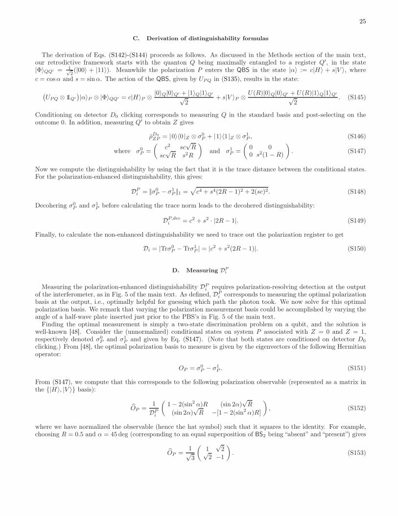
25

C. Derivation of distinguishability formulas

The derivation of Eqs. (S142)-(S144) proceeds as follows. As discussed in the Methods section of the main text,our retrodictive framework starts with the quanton Q being maximally entangled to a register Q′, in the state|Φ〉QQ′ = 1√

2(|00〉 + |11〉). Meanwhile the polarization P enters the QBS in the state |α〉 := c|H〉 + s|V 〉, where

c = cosα and s = sinα. The action of the QBS, given by UPQ in (S135), results in the state:

(UPQ ⊗ 11Q′

)|α〉P ⊗ |Φ〉QQ′ = c|H〉P ⊗ |0〉Q|0〉Q′ + |1〉Q|1〉Q′√

2+ s|V 〉P ⊗ U(R)|0〉Q|0〉Q′ + U(R)|1〉Q|1〉Q′√

2. (S145)

Conditioning on detector D0 clicking corresponds to measuring Q in the standard basis and post-selecting on theoutcome 0. In addition, measuring Q′ to obtain Z gives

ρD0

ZP = |0〉〈0 |Z ⊗ σ0P + |1〉〈1 |Z ⊗ σ1

P , (S146)

where σ0P =

(c2 sc

√R

sc√R s2R

)and σ1

P =

(0 00 s2(1 −R)

). (S147)

Now we compute the distinguishability by using the fact that it is the trace distance between the conditional states.For the polarization-enhanced distinguishability, this gives:

DPi = ||σ0

P − σ1P ||1 =

√c4 + s4(2R− 1)2 + 2(sc)2. (S148)

Decohering σ0P and σ1

P before calculating the trace norm leads to the decohered distinguishability:

DP,deci = c2 + s2 · |2R− 1|. (S149)

Finally, to calculate the non-enhanced distinguishability we need to trace out the polarization register to get

Di = |Trσ0P − Trσ1

P | = |c2 + s2(2R− 1)|. (S150)

D. Measuring DPi

Measuring the polarization-enhanced distinguishability DPi requires polarization-resolving detection at the output

of the interferometer, as in Fig. 5 of the main text. As defined, DPi corresponds to measuring the optimal polarization

basis at the output, i.e., optimally helpful for guessing which path the photon took. We now solve for this optimalpolarization basis. We remark that varying the polarization measurement basis could be accomplished by varying theangle of a half-wave plate inserted just prior to the PBS’s in Fig. 5 of the main text.

Finding the optimal measurement is simply a two-state discrimination problem on a qubit, and the solution iswell-known [48]. Consider the (unnormalized) conditional states on system P associated with Z = 0 and Z = 1,respectively denoted σ0

P and σ1P and given by Eq. (S147). (Note that both states are conditioned on detector D0

clicking.) From [48], the optimal polarization basis to measure is given by the eigenvectors of the following Hermitianoperator:

OP = σ0P − σ1

P . (S151)

From (S147), we compute that this corresponds to the following polarization observable (represented as a matrix inthe |H〉, |V 〉 basis):

OP =1

DPi

(1− 2(sin2 α)R (sin 2α)

√R

(sin 2α)√R −[1− 2(sin2 α)R]

), (S152)

where we have normalized the observable (hence the hat symbol) such that it squares to the identity. For example,choosing R = 0.5 and α = 45 deg (corresponding to an equal superposition of BS2 being “absent” and “present”) gives

OP =1√3

(1

√2√

2 −1

). (S153)