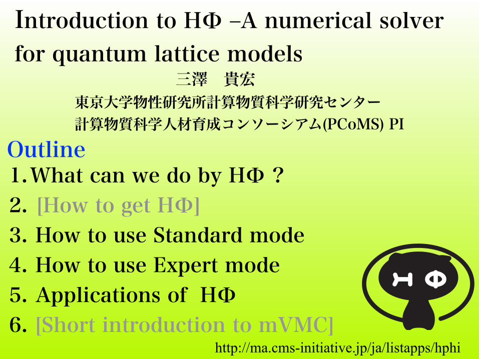
1.What can we do by HΦ ? 2. [How to get HΦ] 3. How to use Standard mode 4. How to use Expert mode 5. Applications of HΦ 6. [Short introduction to mVMC]

Introduction to HΦ ‒A numerical solver for quantum lattice models

Outline

http://ma.cms-initiative.jp/ja/listapps/hphi

三澤　貴宏 東京大学物性研究所計算物質科学研究センター 計算物質科学人材育成コンソーシアム(PCoMS) PI

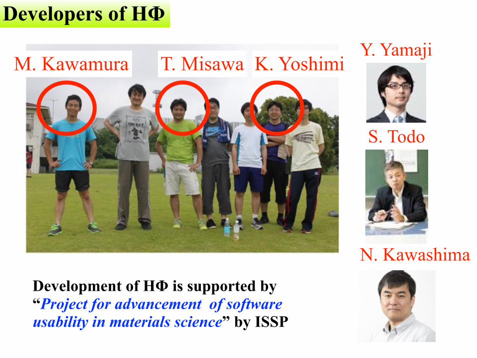
Developers of HΦ

M. Kawamura T. Misawa K. YoshimiY. Yamaji

S. Todo

N. Kawashima

Development of HΦ is supported by “Project for advancement of software usability in materials science” by ISSP

For Hubbard model, spin-S Heisenberg model, Kondo-lattice model with arbitrary one-body and two-body interactions - Full diagonalization - Ground state calculations by Lanczos method - Finite-temperature calculations by thermal pure quantum (TPQ) states - Dynamical properties (optical conductivity ..)

What can we do by HΦ?

maximum system sizes@ ISSP system B (sekirei) - spin 1/2: ~ 40 sites (Sz conserved) - Hubbard model: ~ 20sites (# of particles & Sz conserved)

empty

empty

emptyJ

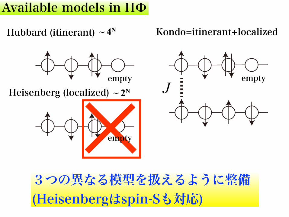
Hubbard (itinerant)

Heisenberg (localized)

Kondo=itinerant+localized

３つの異なる模型を扱えるように整備 (Heisenbergはspin-Sも対応)

~ 4N

~ 2N

Available models in HΦ

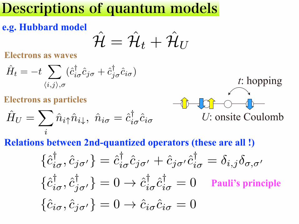
Descriptions of quantum modelse.g. Hubbard model

H = Ht + HU

HU =X

i

ni"ni#, ni� = c†i� ci�

{c†i�, cj�0} = c†i� cj�0 + cj�0 c†i� = �i,j��,�0

{c†i�, c†j�0} = 0 ! c†i� c

†i� = 0

{ci�, cj�0} = 0 ! ci� ci� = 0

Ht = �tX

hi,ji,�

(c†i� cj� + c†j� ci�)

Relations between 2nd-quantized operators (these are all !)

Pauli’s principle

Electrons as waves

Electrons as particles

U: onsite Coulomb

t: hopping

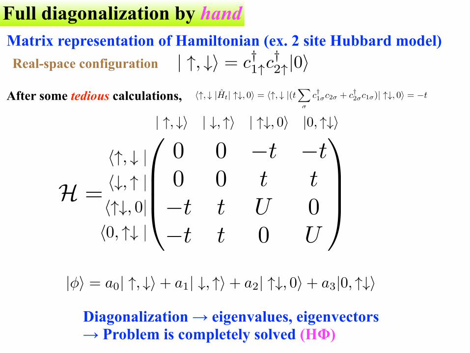
Full diagonalization by handMatrix representation of Hamiltonian (ex. 2 site Hubbard model)

| ", #i = c†1"c†2"|0i

h", # |Ht| "#, 0i = h", # |(tX

�

c†1�c2� + c†2�c1�)| "#, 0i = �t

H =

0

BB@

0 0 �t �t0 0 t t�t t U 0�t t 0 U

1

CCA

| ", #i | #, "i | "#, 0i |0, "#i

Diagonalization → eigenvalues, eigenvectors → Problem is completely solved (HΦ)

Real-space configuration

After some tedious calculations,

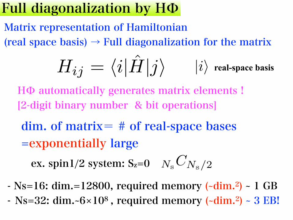
Full diagonalization by HΦ

dim. of matrix＝ # of real-space bases =exponentially largeex. spin1/2 system: Sz=0

Matrix representation of Hamiltonian (real space basis) → Full diagonalization for the matrix

Hij = hi|H|ji

NsCNs/2

- Ns=16: dim.=12800, required memory (~dim.2) ~ 1 GB - Ns=32: dim.~6×108 , required memory (~dim.2) ~ 3 EB!

|ii real-space basis

HΦ automatically generates matrix elements ! [2-digit binary number & bit operations]

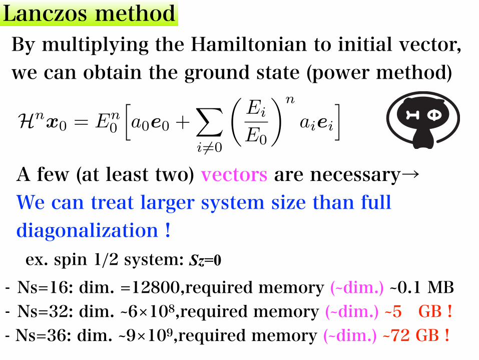
Lanczos methodBy multiplying the Hamiltonian to initial vector, we can obtain the ground state (power method)

A few (at least two) vectors are necessary→ We can treat larger system size than full diagonalization !

Hnx0 = En

0

ha0e0 +

X

i 6=0

✓Ei

E0

◆n

aieii

- Ns=16: dim. =12800,required memory (~dim.) ~0.1 MB - Ns=32: dim. ~6×108,required memory (~dim.) ~5 GB ! - Ns=36: dim. ~9×109,required memory (~dim.) ~72 GB !

ex. spin 1/2 system: Sz=0

waking sleeping

Meaning of name & logo

+Φ=

- Multiplying H to Φ (HΦ) - This cat means wave function in two ways cat is a symbol of superposition.. (Schrödinger’s cat)

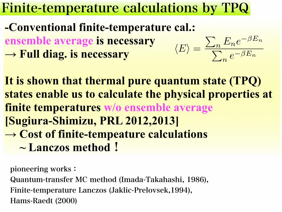
-Conventional finite-temperature cal.: ensemble average is necessary → Full diag. is necessary

It is shown that thermal pure quantum state (TPQ) states enable us to calculate the physical properties at finite temperatures w/o ensemble average [Sugiura-Shimizu, PRL 2012,2013] → Cost of finite-tempeature calculations ~ Lanczos method！

Finite-temperature calculations by TPQ

pioneering works： Quantum-transfer MC method (Imada-Takahashi, 1986), Finite-temperature Lanczos (Jaklic-Prelovsek,1994), Hams-Raedt (2000)

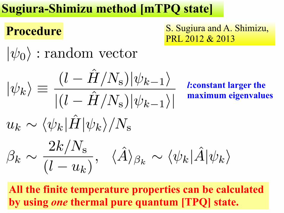
Sugiura-Shimizu method [mTPQ state]

All the finite temperature properties can be calculated by using one thermal pure quantum [TPQ] state.

Procedure S. Sugiura and A. Shimizu, PRL 2012 & 2013

l:constant larger the maximum eigenvalues

| 0i : random vector

| ki ⌘(l � ˆH/Ns)| k�1i|(l � ˆH/Ns)| k�1i|

uk ⇠ h k| ˆH| ki/Ns

�k ⇠ 2k/Ns

(l � uk), h ˆAi�k ⇠ h k| ˆA| ki

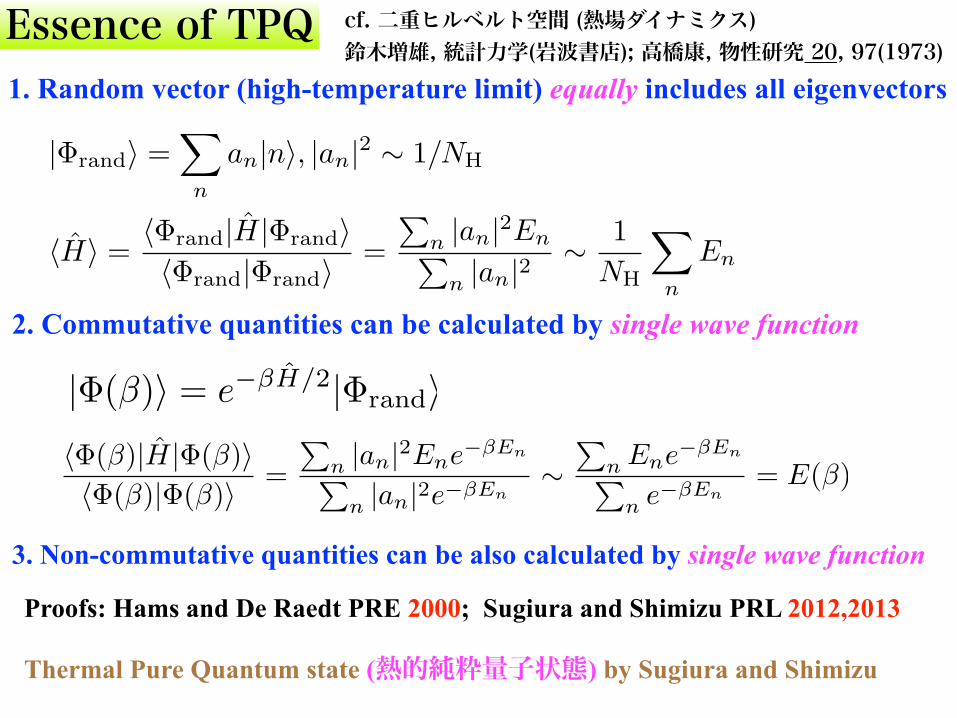
Essence of TPQ1. Random vector (high-temperature limit) equally includes all eigenvectors

2. Commutative quantities can be calculated by single wave function

3. Non-commutative quantities can be also calculated by single wave function

Proofs: Hams and De Raedt PRE 2000; Sugiura and Shimizu PRL 2012,2013

Thermal Pure Quantum state (熱的純粋量子状態) by Sugiura and Shimizu

cf. 二重ヒルベルト空間 (熱場ダイナミクス) 鈴木増雄, 統計力学(岩波書店); 高橋康, 物性研究 20, 97(1973)

Drastic reduction of numerical cost

Heisenberg model, 32 sites, Sz=0

Full diagonalization: Dimension of Hamiltonian ~ 108×108　 Memory ~ 3E Byte → Almost impossible. 　

TPQ method: Only two vectors are required: dimension of vector ~ 108×108　 Memory ~ 10 G Byte → Possible even in lab’s cluster machine ! 　

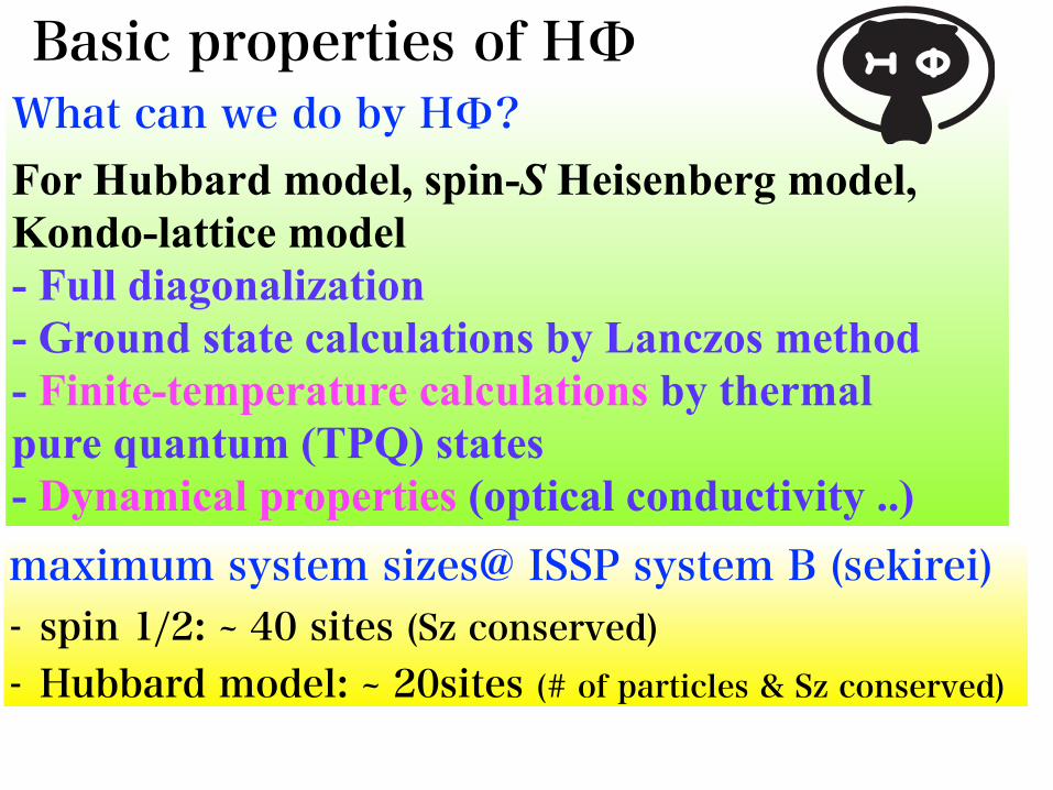
What can we do by HΦ? For Hubbard model, spin-S Heisenberg model, Kondo-lattice model - Full diagonalization - Ground state calculations by Lanczos method - Finite-temperature calculations by thermal pure quantum (TPQ) states - Dynamical properties (optical conductivity ..)

Basic properties of HΦ

maximum system sizes@ ISSP system B (sekirei) - spin 1/2: ~ 40 sites (Sz conserved) - Hubbard model: ~ 20sites (# of particles & Sz conserved)

Let’s get HΦ !

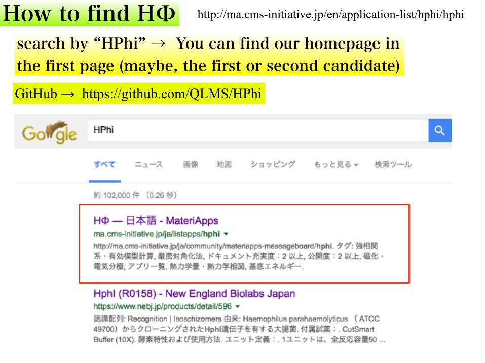
How to find HΦsearch by “HPhi” → You can find our homepage in the first page (maybe, the first or second candidate)

http://ma.cms-initiative.jp/en/application-list/hphi/hphi

GitHub → https://github.com/QLMS/HPhi

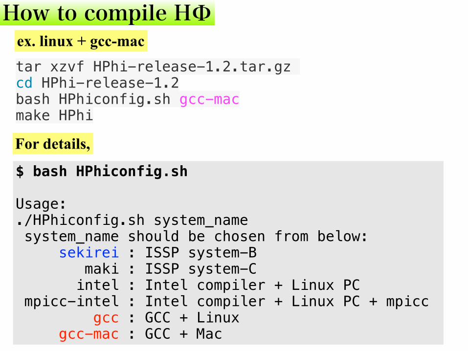
How to compile HΦ

tar xzvf HPhi-release-1.2.tar.gz cd HPhi-release-1.2 bash HPhiconfig.sh gcc-mac make HPhi

ex. linux + gcc-mac

$ bash HPhiconfig.sh

Usage: ./HPhiconfig.sh system_name system_name should be chosen from below: sekirei : ISSP system-B maki : ISSP system-C intel : Intel compiler + Linux PC mpicc-intel : Intel compiler + Linux PC + mpicc gcc : GCC + Linux gcc-mac : GCC + Mac

For details,

Let’s start HΦ ! (Standard mode)

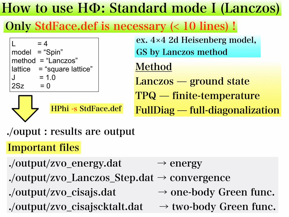
How to use HΦ: Standard mode I (Lanczos)Only StdFace.def is necessary (< 10 lines) !

L = 4 model = “Spin” method = “Lanczos” lattice = “square lattice” J = 1.0 2Sz = 0

HPhi -s StdFace.def

./ouput : results are output

./output/zvo_energy.dat　　　 → energy

./output/zvo_Lanczos_Step.dat → convergence

./output/zvo_cisajs.dat → one-body Green func.

./output/zvo_cisajscktalt.dat → two-body Green func.

Important files

ex. 4×4 2d Heisenberg model, GS by Lanczos method

Method Lanczos ground state TPQ finite-temperature FullDiag full-diagonalization

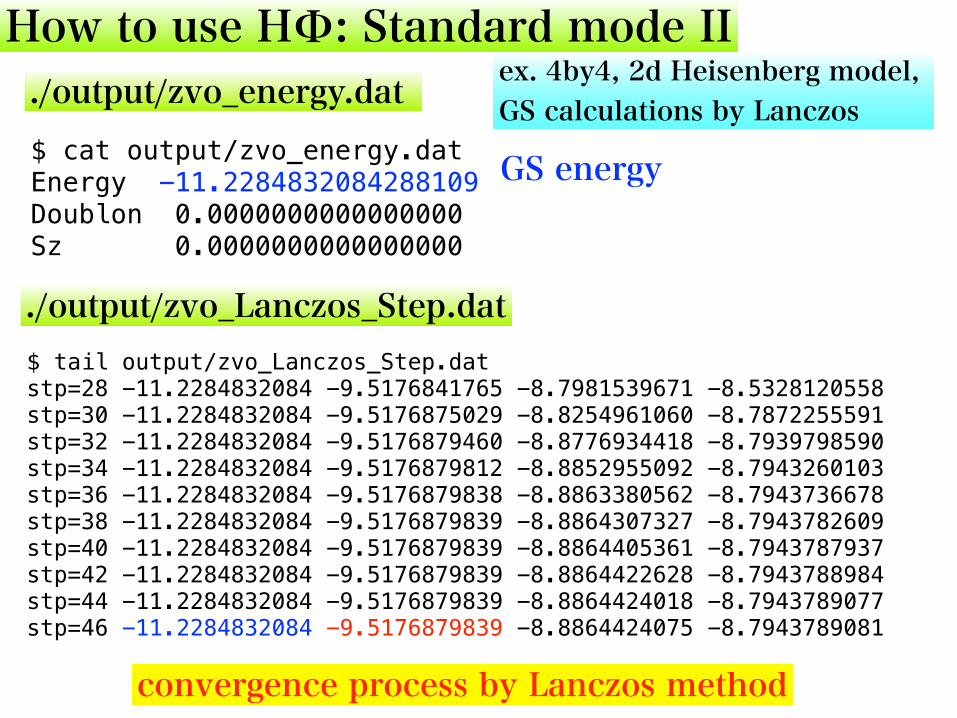
How to use HΦ: Standard mode II

$ cat output/zvo_energy.dat Energy -11.2284832084288109 Doublon 0.0000000000000000 Sz 0.0000000000000000

$ tail output/zvo_Lanczos_Step.dat stp=28 -11.2284832084 -9.5176841765 -8.7981539671 -8.5328120558 stp=30 -11.2284832084 -9.5176875029 -8.8254961060 -8.7872255591 stp=32 -11.2284832084 -9.5176879460 -8.8776934418 -8.7939798590 stp=34 -11.2284832084 -9.5176879812 -8.8852955092 -8.7943260103 stp=36 -11.2284832084 -9.5176879838 -8.8863380562 -8.7943736678 stp=38 -11.2284832084 -9.5176879839 -8.8864307327 -8.7943782609 stp=40 -11.2284832084 -9.5176879839 -8.8864405361 -8.7943787937 stp=42 -11.2284832084 -9.5176879839 -8.8864422628 -8.7943788984 stp=44 -11.2284832084 -9.5176879839 -8.8864424018 -8.7943789077 stp=46 -11.2284832084 -9.5176879839 -8.8864424075 -8.7943789081

./output/zvo_energy.dat　　　

./output/zvo_Lanczos_Step.dat

GS energy

convergence process by Lanczos method

ex. 4by4, 2d Heisenberg model, GS calculations by Lanczos

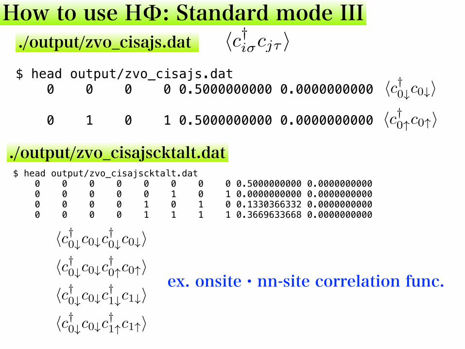
How to use HΦ: Standard mode III./output/zvo_cisajs.dat

./output/zvo_cisajscktalt.dat

$ head output/zvo_cisajs.dat 0 0 0 0 0.5000000000 0.0000000000 0 1 0 1 0.5000000000 0.0000000000

$ head output/zvo_cisajscktalt.dat 0 0 0 0 0 0 0 0 0.5000000000 0.0000000000 0 0 0 0 0 1 0 1 0.0000000000 0.0000000000 0 0 0 0 1 0 1 0 0.1330366332 0.0000000000 0 0 0 0 1 1 1 1 0.3669633668 0.0000000000

hc†i�cj⌧ i

hc†0"c0"i

hc†0#c0#i

hc†0#c0#c†0#c0#i

hc†0#c0#c†0"c0"i

hc†0#c0#c†1#c1#i

hc†0#c0#c†1"c1"i

ex. onsite・nn-site correlation func.

How to use HΦ: Standard mode IVHPhi/samples/Standard/　 StdFace.def for Hubbard model, Heisenberg model, Kitaev model, Kondo-lattice model

By changing StdFace.def slightly, you can easily perform the calculations for different models.

Cautions： - Do not input too large system size (upper limit@laptop: spin 1/2→24 sites, Hubbard model 12 sites) - Lanczos method is unstable for too small size (dim. > 1000) -TPQ method does not work well for small size (dim. > 1000)

Expert mode !

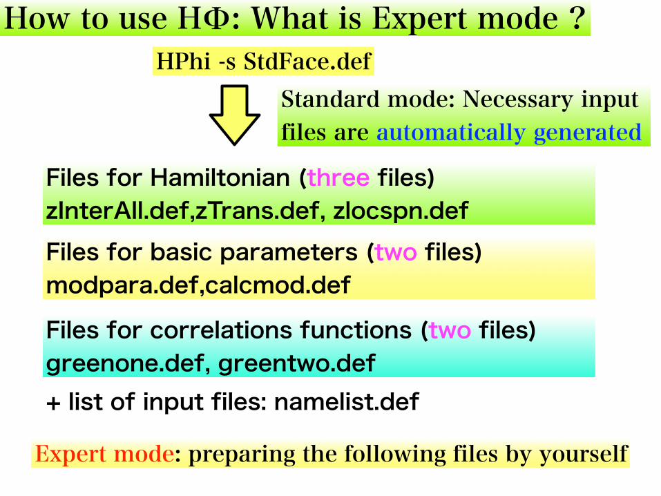
How to use HΦ: What is Expert mode ?

Files for Hamiltonian (three files) zInterAll.def,zTrans.def, zlocspn.defFiles for basic parameters (two files) modpara.def,calcmod.def

Standard mode: Necessary input files are automatically generated

Files for correlations functions (two files) greenone.def, greentwo.def

HPhi -s StdFace.def

+ list of input files: namelist.def

Expert mode: preparing the following files by yourself

How to use HΦ: What is Expert mode ?

HPhi -e namelist.def

Expert mode: preparing the following files by yourself

execute following command

Files for Hamiltonian (three files) zInterAll.def,zTrans.def, zlocspn.defFiles for basic parameters (two files) modpara.def,calcmod.def

Files for correlations functions (two files) greenone.def, greentwo.def

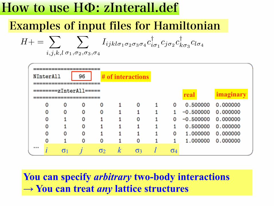
How to use HΦ: zInterall.def

You can specify arbitrary two-body interactions → You can treat any lattice structures

Examples of input files for Hamiltonian

# of interactions

real imaginary

i σ1 j σ2 k σ3 l σ4

H+ =X

i,j,k,l

X

�1,�2,�3,�4

Iijkl�1�2�3�4c†i�1

cj�2c†k�3

cl�4

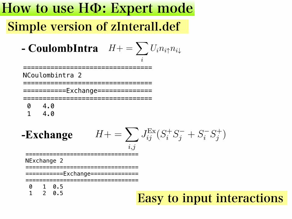
How to use HΦ: Expert modeSimple version of zInterall.def

- CoulombIntra

-Exchange

4.2 エキスパートモード用入力ファイル 49

4.2.7 CoulombIntra指定ファイルオンサイトクーロン相互作用をハミルトニアンに付け加えます (S = 1/2の系で

のみ使用可能、ver. 0.2ではMPI非対応)。付け加える項は以下で与えられます。

H+ =!

i

Uini↑ni↓ (4.12)

以下にファイル例を記載します。✓ ✏======================NCoulombIntra 6==============================i_0LocSpn_1IteElc ============================

0 4.0000001 4.0000002 4.0000003 4.0000004 4.0000005 4.000000✒ ✑

ファイル形式以下のように行数に応じ異なる形式をとります。

• 1行: ヘッダ (何が書かれても問題ありません)。

• 2行: [string01] [int01]

• 3-5行: ヘッダ (何が書かれても問題ありません)。

• 6行以降: [int02] [double01]

パラメータ• [string01]

形式 : string型 (空白不可)

説明 : オンサイトクーロン相互作用の総数のキーワード名を指定します (任意)。

• [int01]

形式 : int型 (空白不可)

説明 : オンサイトクーロン相互作用の総数を指定します。

• [int02]

形式 : int型 (空白不可)

説明 : サイト番号を指定する整数。0以上 Nsite未満で指定します。

4.2 エキスパートモード用入力ファイル 57

4.2.11 Exchange指定ファイルExchangeカップリングをハミルトニアンに付け加えます (S = 1/2の系でのみ

使用可能、ver. 0.2ではMPI非対応)。電子系の場合には

H+ =!

i,j

JExij (c†i↑cj↑c

†j↓ci↓ + c†i↓cj↓c

†j↑ci↑) (4.16)

が付け加えられ、スピン系の場合には

H+ =!

i,j

JExij (S+

i S−j + S−

i S+j ) (4.17)

が付け加えられます。スピン系の (S+i S

−j + S−

i S+j )を電子系の演算子で書き直すと、

−(c†i↑cj↑c†j↓ci↓ + c†i↓cj↓c

†j↑ci↑) となることに注意して下さい。以下にファイル例を記載

します。✓ ✏======================NExchange 6==============================Exchange ============================

0 1 0.500001 2 0.500002 3 0.500003 4 0.500004 5 0.500005 0 0.50000✒ ✑

ファイル形式以下のように行数に応じ異なる形式をとります。

• 1行: ヘッダ (何が書かれても問題ありません)。

• 2行: [string01] [int01]

• 3-5行: ヘッダ (何が書かれても問題ありません)。

• 6行以降: [int02] [int03] [double01]

パラメータ• [string01]

形式 : string型 (空白不可)

説明 : Exchangeカップリングの総数のキーワード名を指定します (任意)。

================================= NExchange 2 ================================= ===========Exchange============== ================================= 0 1 0.5 1 2 0.5

================================= NCoulombintra 2 ================================= ===========Exchange============== ================================= 0 4.0 1 4.0

Easy to input interactions

Applications of HΦ!

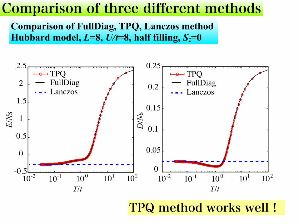
Comparison of three different methodsComparison of FullDiag, TPQ, Lanczos method Hubbard model, L=8, U/t=8, half filling, Sz=0

-0.5

0

0.5

1

1.5

2

2.5

0

0.05

0.1

0.15

0.2

0.25

10 10 10 10 10-2 -1 0 1 2 10 10 10 10 10-2 -1 0 1 2

D/N

s

E/N

s

TPQFullDiagLanczos

TPQFullDiagLanczos

T/t T/t

TPQ method works well !

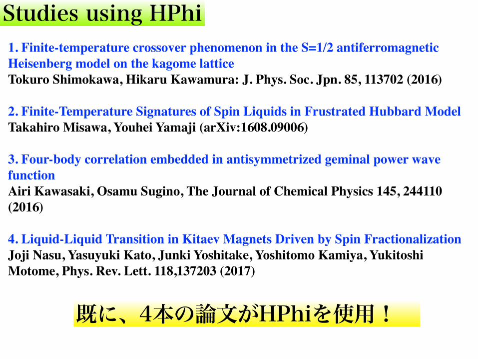
Studies using HPhi

既に、4本の論文がHPhiを使用！

1. Finite-temperature crossover phenomenon in the S=1/2 antiferromagnetic Heisenberg model on the kagome latticeTokuro Shimokawa, Hikaru Kawamura: J. Phys. Soc. Jpn. 85, 113702 (2016)

2. Finite-Temperature Signatures of Spin Liquids in Frustrated Hubbard Model Takahiro Misawa, Youhei Yamaji (arXiv:1608.09006)

3. Four-body correlation embedded in antisymmetrized geminal power wave function Airi Kawasaki, Osamu Sugino, The Journal of Chemical Physics 145, 244110 (2016)

4. Liquid-Liquid Transition in Kitaev Magnets Driven by Spin Fractionalization Joji Nasu, Yasuyuki Kato, Junki Yoshitake, Yoshitomo Kamiya, Yukitoshi Motome, Phys. Rev. Lett. 118,137203 (2017)

HPhiの使い方0. 汎用性を優先して、速度・サイズなどは犠牲にしている部分がある→対角化(Lanczos法)での世界最大の計算は（現段階では)無理

1. spin 1/2 36 sites, Hubbard 18 sites程度までの有限・励起状態計算 は比較的すぐできる。とくに、エントロピーが低温まで残る フラスレート系が得意 [論文 1(kagome),2(t-t’ Hubbard)]。

2. 平均場計算などで「面白い」ことがおきることを確認 →HPhiでその結果を確認する[論文4(extended Kitaev model)]

3. 新手法開発した際の精度確認[論文3(extended geminal wave functions)] ~20 site Hubbard model

4. 新奇物質に対する現実的な有効模型の妥当性の確認,物性予測

(励起状態、有限温度、動的物理量)[Na2IrO3, Yamaji et al.]

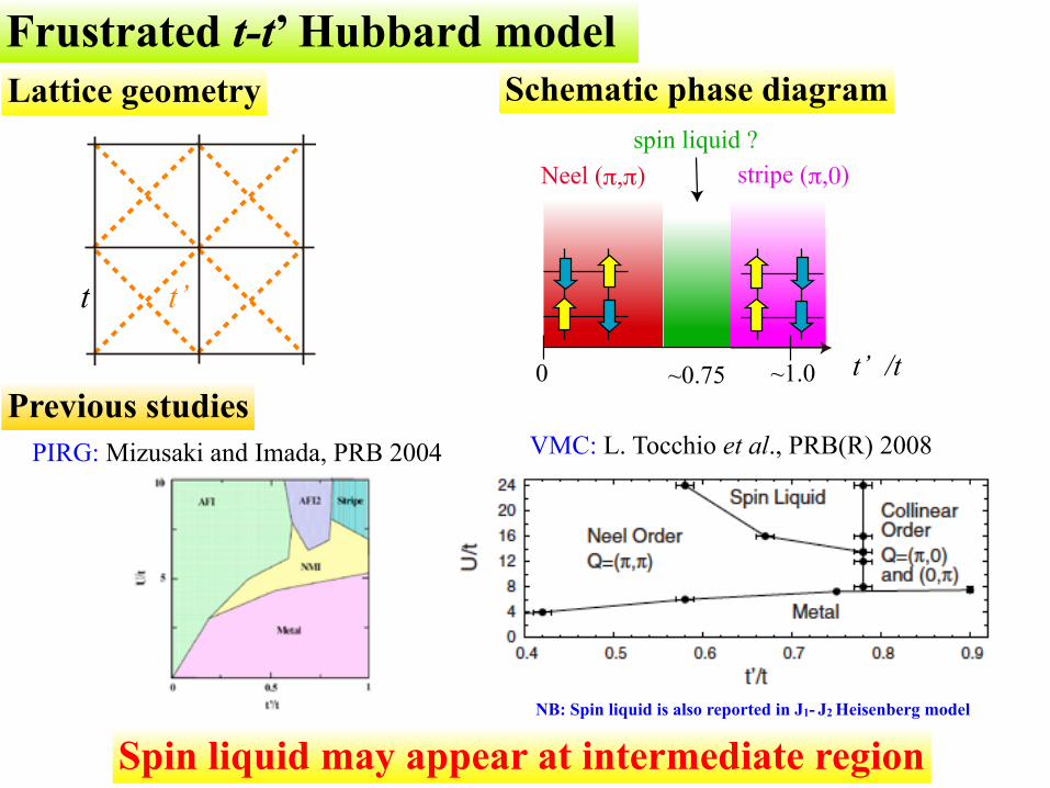
Frustrated t-t’ Hubbard model

Spin liquid may appear at intermediate region

PIRG: Mizusaki and Imada, PRB 2004 VMC: L. Tocchio et al., PRB(R) 2008

t t’

t’ /t0

Neel (π,π) stripe (π,0)spin liquid ?

~1.0~0.75

Lattice geometry Schematic phase diagram

Previous studies

NB: Spin liquid is also reported in J1- J2 Heisenberg model

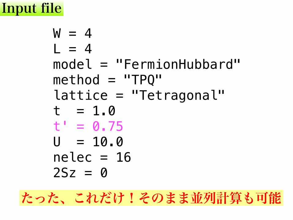
Input file

W = 4 L = 4 model = "FermionHubbard" method = "TPQ" lattice = "Tetragonal" t = 1.0 t' = 0.75 U = 10.0 nelec = 16 2Sz = 0

たった、これだけ！そのまま並列計算も可能

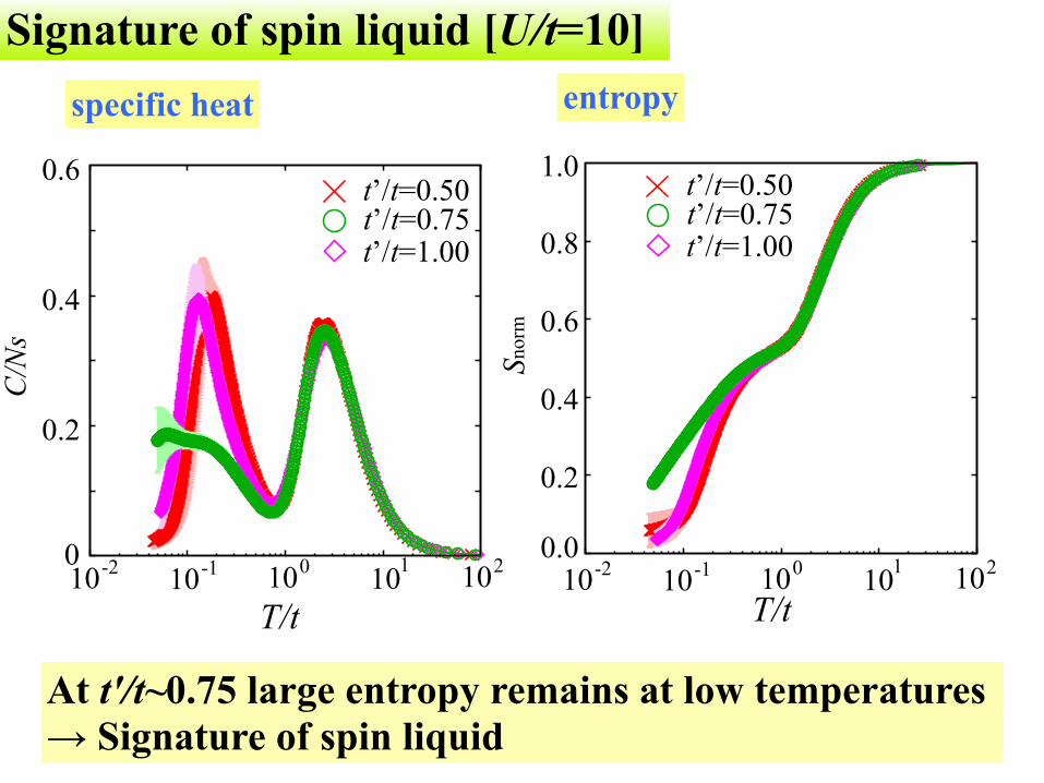
At t'/t~0.75 large entropy remains at low temperatures → Signature of spin liquid

Signature of spin liquid [U/t=10]specific heat entropy

0

0.2

0.4

0.6

C/Ns

T/t

Snor

m

t’/t=0.50t’/t=0.75t’/t=1.00

t’/t=0.50t’/t=0.75t’/t=1.00

0.0

0.2

0.4

0.6

0.8

1.0

10-2 10-1 100 101 102 10-2 10-1 100 101 102

T/t

Available system size in SC@ISSPISSP system B (sekirei)✓fat node: 1node (40 cores) memory/node = 1TB、 up to 2nodes → ~2TB ✓cpu node: 1node (24cores) memory/node=120GB, up to 144nodes→~17TB

SC@ISSP: - It is very easy (cheap) to perform the calculations up to spin 1/2 = 32 sites, Hubbard = 16 sites

- It is possible (but expensive !) to perform the calculations up to spin 1/2 40 sites, Hubbard 20 sites (state-of-the-art calculations 5-10 years ago)

If you have any questions, please join HPhi ML and ask questions

Summary- Explained basic properties of HΦ: Full diagonalization, Lanzcos method, TPQ method for Heisenberg, Hubbard, Kondo, Kitaev model ….

- Explained how to use HΦ: Very easy to start calculations by using Standard mode Easy to treat general Hamiltonians by using Expert mode

- Shown applications of HΦ: Found the finite-temperature signature of QSL in t-t’ Hubbard model