FUNDAMENTAL PROPERTIES OF

ACCRETING COMPACT OBJECTS

by

Jennifer L. Blum

A dissertation submitted in partial fulfillmentof the requirements for the degree of

Doctor of Philosophy(Astronomy and Astrophysics)in The University of Michigan

2011

Doctoral Committee:

Associate Professor Jon M. Miller, ChairProfessor Lee W. HartmannProfessor Timothy A. McKayAssistant Professor Mateusz Ruszkowski

Copyright c©Jennifer L. Blum

All Rights Reserved2011

For my parents, who have always made me feel significant in the Universe

ii

ACKNOWLEDGMENTS

This dissertation is the result of four years of research at the University of Michigan

under the tutelage of my colleagues in the Department of Astronomy. First and

foremost, I would like to thank my advisor Jon Miller who has been the most amazing

and supportive mentor. During my time as a graduate student, he has gone above

and beyond the call of duty (including wearing a Yankees cap) as an advisor to help

me succeed in my academic endeavors. Under Jon Miller’s teaching and guidance,

I have gained invaluable experience that I will carry with me throughout my career

and life. Additionally, I am grateful towards my thesis committee, Lee Hartmann,

Tim McKay, and Mateusz Ruszkowski who, without their advice and support, this

work would not be possible.

A huge thanks to everyone in the Department of Astronomy, most notably Doug

Richstone, Joel Bregman, Ed Cackett, and Mark Reynolds for their tremendous help

and support. Also, a huge thank you to Nuria Calvet for her unyielding support

throughout the hardships of graduate school. Also, thank you to Roy Bonser who

has gotten me out of more than one technical hardship.

I am also grateful to the graduate students (both past and present) for their

kindness and help. Life in Ann Arbor would not be nearly as fun without them.

Specifically, thank you to Jess Werk, Catherine Espaillat, and Sarah Ragan who

have been my inspiration and have helped me to become strong and independent.

A thank you to my first true academic sister Laura Ingleby (Team Bling!) for her

companionship, support, and fantastic sense of fashion. A thank you to my office

mate Shannon Schmoll for making me see how fun (and silly!) life can be as well as

sharing my love of British television and all things Winchester. A thank you to Joel

Lamb and Kiwi Davis who share my enthusiasm for anime, video games, and seeing

iii

the (sometimes twisted) humor in life.

Lastly, I would like to thank my family. To my mom and dad, specifically, I extend

my deepest thanks for their love and support. They have helped me through it all

and will always be my truest source of happiness and inspiration.

iv

PREFACE

Chapters 2 and 4 of this thesis are based on publications in The Astrophysical

Journal and are reproduced here with permission (Blum et al. 2009, 2010). They

have been slightly altered from their original published forms to fit the thesis format.

Chapter 3 is based on work in progress to be published in The Astrophysical Journal

(Blum et al. in preparation).

v

CONTENTS

DEDICATION . . . . . . . . . . . . . . . . . . . . . . . . . . . . . . . . . . . . . . . . . . . . . . ii

ACKNOWLEDGMENTS . . . . . . . . . . . . . . . . . . . . . . . . . . . . . . . . . . . . . . iii

PREFACE . . . . . . . . . . . . . . . . . . . . . . . . . . . . . . . . . . . . . . . . . . . . . . . . . v

LIST OF FIGURES . . . . . . . . . . . . . . . . . . . . . . . . . . . . . . . . . . . . . . . . . . viii

LIST OF TABLES . . . . . . . . . . . . . . . . . . . . . . . . . . . . . . . . . . . . . . . . . . . x

ABSTRACT . . . . . . . . . . . . . . . . . . . . . . . . . . . . . . . . . . . . . . . . . . . . . . . xi

CHAPTER

1 Introduction . . . . . . . . . . . . . . . . . . . . . . . . . . . . . . . . . . . . . . . . . 1

1.1 A Brief History on the Idea and Discovery of Neutron Stars and

Black Holes . . . . . . . . . . . . . . . . . . . . . . . . . . . . . . . . . . . . . . 4

1.2 The Fe K Emission Line . . . . . . . . . . . . . . . . . . . . . . . . . . . . . 7

1.3 Spectral States . . . . . . . . . . . . . . . . . . . . . . . . . . . . . . . . . . . . 10

1.3.1 QPOs and Neutron Star Equation of State . . . . . . . . . . 16

1.4 Disk Winds and Jets . . . . . . . . . . . . . . . . . . . . . . . . . . . . . . . . 17

1.5 The Suzaku X-ray Satellite . . . . . . . . . . . . . . . . . . . . . . . . . . . 22

1.6 Thesis Overview . . . . . . . . . . . . . . . . . . . . . . . . . . . . . . . . . . . 25

1.6.1 Black Hole Spin . . . . . . . . . . . . . . . . . . . . . . . . . . . . . 27

1.6.2 Inner Disk Radius and Neutron Star Radius . . . . . . . . . 27

1.6.3 Disk Winds and Jets . . . . . . . . . . . . . . . . . . . . . . . . . 27

1.6.4 Conclusions . . . . . . . . . . . . . . . . . . . . . . . . . . . . . . . . 28

2 Measuring the Spin of GRS 1915+105 with Relativistic Disk

Reflection . . . . . . . . . . . . . . . . . . . . . . . . . . . . . . . . . . . . . . . . . . . . 29

2.1 Introduction . . . . . . . . . . . . . . . . . . . . . . . . . . . . . . . . . . . . . . 29

vi

2.2 Data Reduction . . . . . . . . . . . . . . . . . . . . . . . . . . . . . . . . . . . 30

2.3 Data Analysis and Results . . . . . . . . . . . . . . . . . . . . . . . . . . . 31

2.4 Discussion . . . . . . . . . . . . . . . . . . . . . . . . . . . . . . . . . . . . . . . 36

3 A Look at the Inner Disk in the Neutron Star Low-Mass X-ray

Binary 4U 1636-53 with Suzaku . . . . . . . . . . . . . . . . . . . . . . . . . . 48

3.1 Introduction . . . . . . . . . . . . . . . . . . . . . . . . . . . . . . . . . . . . . . 48

3.2 Data Reduction . . . . . . . . . . . . . . . . . . . . . . . . . . . . . . . . . . . 50

3.2.1 Suzaku Data Reduction . . . . . . . . . . . . . . . . . . . . . . . 50

3.2.2 RXTE Data Reduction . . . . . . . . . . . . . . . . . . . . . . . 52

3.3 Data Analysis and Results . . . . . . . . . . . . . . . . . . . . . . . . . . . . 53

3.3.1 State Classification of Observations . . . . . . . . . . . . . . . 53

3.3.2 Spectral Modeling . . . . . . . . . . . . . . . . . . . . . . . . . . . 53

3.3.3 kHz QPO Results . . . . . . . . . . . . . . . . . . . . . . . . . . . 64

3.4 Discussion . . . . . . . . . . . . . . . . . . . . . . . . . . . . . . . . . . . . . . . 64

3.4.1 The Inner Disk Radius and State Transitions . . . . . . . . 65

3.4.2 Alternative Possibilities for State Transitions . . . . . . . . 68

3.4.3 Neutron Star Equation of State . . . . . . . . . . . . . . . . . . 68

3.4.4 Conclusions . . . . . . . . . . . . . . . . . . . . . . . . . . . . . . . . 69

4 Suzaku Observations of the Black Hole H1743-322 in Outburst 80

4.1 Introduction . . . . . . . . . . . . . . . . . . . . . . . . . . . . . . . . . . . . . . 80

4.2 Data Reduction . . . . . . . . . . . . . . . . . . . . . . . . . . . . . . . . . . . 81

4.3 Data Analysis and Results . . . . . . . . . . . . . . . . . . . . . . . . . . . . 82

4.4 Discussion . . . . . . . . . . . . . . . . . . . . . . . . . . . . . . . . . . . . . . . 85

5 Conclusions . . . . . . . . . . . . . . . . . . . . . . . . . . . . . . . . . . . . . . . . . . 93

5.1 Summary of Results from Individual Chapters . . . . . . . . . . . . . . 93

5.1.1 Chapter 2 Summary . . . . . . . . . . . . . . . . . . . . . . . . . . 93

5.1.2 Chapter 3 Summary . . . . . . . . . . . . . . . . . . . . . . . . . . 95

5.1.3 Chapter 4 Summary . . . . . . . . . . . . . . . . . . . . . . . . . . 96

BIBLIOGRAPHY . . . . . . . . . . . . . . . . . . . . . . . . . . . . . . . . . . . . . . . . . . . . 99

vii

LIST OF FIGURES

Figure

1.1 Artist rendition of a black hole X-ray binary . . . . . . . . . . . . . . . . . . . 5

1.2 Compilation of effects that create the observed iron line profile . . . . . . 11

1.3 Correlation between black hole spin and the ISCO . . . . . . . . . . . . . . 12

1.4 Black hole LMXB spectral states . . . . . . . . . . . . . . . . . . . . . . . . . . . 18

1.5 Two kHz QPO peaks in a power spectrum . . . . . . . . . . . . . . . . . . . . 19

1.6 Neutron star equation of state . . . . . . . . . . . . . . . . . . . . . . . . . . . . . 20

1.7 Artist rendition of Suzaku . . . . . . . . . . . . . . . . . . . . . . . . . . . . . . . . 25

1.8 Internal schematic of Suzaku . . . . . . . . . . . . . . . . . . . . . . . . . . . . . . 26

2.1 Data/model ratio obtained with a simple power-law model . . . . . . . . . 42

2.2 Data/model ratio obtained with a broken power-law model . . . . . . . . 43

2.3 Best-fit spectrum found through modeling of the iron line at 6.4 keV . 43

2.4 Change in the goodness-of-fit statistic as a function of the black hole

spin parameter using the pexriv model . . . . . . . . . . . . . . . . . . . . . . 44

2.5 Best-fit spectrum found through modeling of the iron line at 6.4 keV . 44

2.6 Change in the goodness-of-fit statistic as a function of the black hole

spin parameter using the reflionx model . . . . . . . . . . . . . . . . . . . . 45

2.7 Inclination versus spin contour plot for GRS 1915+105 using the pexriv

model . . . . . . . . . . . . . . . . . . . . . . . . . . . . . . . . . . . . . . . . . . . . . . 46

2.8 Inclination versus spin contour plot for GRS 1915+105 using the reflionx

model . . . . . . . . . . . . . . . . . . . . . . . . . . . . . . . . . . . . . . . . . . . . . . 47

3.1 Long-term hardness, CD, and hardness-intensity curves . . . . . . . . . . . 74

3.2 Iron line profiles . . . . . . . . . . . . . . . . . . . . . . . . . . . . . . . . . . . . . . . 75

viii

3.3 Data/model ratios of the Suzaku spectra of 4U 1636-53 . . . . . . . . . . . 76

3.4 The diskline model and components . . . . . . . . . . . . . . . . . . . . . . . 77

3.5 Blackbody and disk blackbody plots . . . . . . . . . . . . . . . . . . . . . . . . 78

3.6 Iron line flux plots . . . . . . . . . . . . . . . . . . . . . . . . . . . . . . . . . . . . . 79

4.1 Light curve and hardness ratio for the 2003 and 2008 outburst of

H1743-322 . . . . . . . . . . . . . . . . . . . . . . . . . . . . . . . . . . . . . . . . . . . 90

4.2 Suzaku spectrum of H1743-322 fitted with a broken power-law model . 91

4.3 Data/model ratio for the broken power-law model . . . . . . . . . . . . . . . 91

4.4 Data/model ratio from 3−9 keV for the broken power-law model . . . . 92

ix

LIST OF TABLES

Table

2.1 XSPEC pexriv model . . . . . . . . . . . . . . . . . . . . . . . . . . . . . . . . . . . 41

2.2 XSPEC reflionx model . . . . . . . . . . . . . . . . . . . . . . . . . . . . . . . . . . 42

3.1 Suzaku observations of 4U 1636-53 . . . . . . . . . . . . . . . . . . . . . . . . . . 71

3.2 Suzaku and RXTE observations of 4U 1636-53 . . . . . . . . . . . . . . . . . 71

3.3 Gaussian parameters . . . . . . . . . . . . . . . . . . . . . . . . . . . . . . . . . . . . 71

3.4 Phenomenological parameters . . . . . . . . . . . . . . . . . . . . . . . . . . . . . . 72

3.5 Reflection Model Parameters . . . . . . . . . . . . . . . . . . . . . . . . . . . . . . 73

4.1 Broken power-law model parameters . . . . . . . . . . . . . . . . . . . . . . . . . 88

4.2 Comptonization model parameters . . . . . . . . . . . . . . . . . . . . . . . . . . 88

4.3 X-ray absorption lines upper limits . . . . . . . . . . . . . . . . . . . . . . . . . . 88

4.4 X-ray emission line detection . . . . . . . . . . . . . . . . . . . . . . . . . . . . . . 89

x

ABSTRACT

Galactic accreting compact objects, such as stellar-mass black holes and neutron

stars, can give us a unique perspective into the behavior of matter in extreme con-

ditions. However, the exact nature of accretion onto these objects is not yet well

understood. X-ray studies provide us with a means to observe the innermost re-

gions around these objects and to explore our theories of general relativistic physics.

Through X-ray analyses we can constrain the physical parameters necessary to make

logical deductions regarding compact object properties, such as disk winds, relativis-

tic jets, the Kerr metric, and the neutron star equation of state.

Here we present spectral modeling results from three accreting X-ray binaries.

Specifically, we analyze Suzaku spectra from two stellar-mass black hole X-ray bina-

ries, GRS 1915+105 and H1743-322, and one neutron star X-ray binary, 4U 1636-53.

For GRS 1915+105 and 4U 1636-53, we use the relativistic iron line, which is part of

a reflection spectrum, as a diagnostic for measuring black hole spin and neutron star

radius, respectively. We find that while we can exclude a spin of zero at the 2σ level

of confidence for GRS 1915+105, data selection and disk reflection modeling nuances

can be important when estimating the spin value. For 4U 1636-53, we provide upper

limits on the neutron star radius by estimating the radial extent of the inner accretion

disk, which are important for constraining models for the neutron star equation of

state. Moreover, when testing for the presence of disk winds in H1743-322 (which are

key to understanding the nature of accretion disk outflow), we do not detect Fe XXV

or Fe XXVI absorption lines in its spectra of H1743-322; implying that disk winds

may be state dependent.

xi

CHAPTER 1

Introduction

Neutron stars and black holes can give us a unique perspective into the behavior

of matter in extreme conditions. Neutron stars, for example, represent the densest

forms of matter in the Universe (at a mean density ≤ 1015g cm−3, all of humanity

could fit into a cube 1 cm on each side; Shapiro & Teukolsky 1983) while black holes

have such strong gravitational forces that light cannot escape once it has passed the

event horizon. Thus, such objects have fascinated astronomers for decades due to

their “extreme” nature and our inability to replicate such conditions in a laboratory

setting.

But, what are these objects and how do they form? A star’s evolution is solely

determined by its initial mass. As such, neutron stars and black holes represent the

two possible end points of a massive star’s life. When a massive star (>8M⊙) runs

out of nuclear fuel, it can no longer support itself against gravity and undergoes a

gravitational collapse. As a result, the star experiences a “violent death” in the form

of a supernova explosion (see e.g. Tauris & van den Heuvel 2006). Two possibilities

exist for what remains after such an explosion: a neutron star or a black hole. A

neutron star is created when the core of a massive star passes the Chandrasekhar limit

(∼ 1.4M⊙) and undergoes gravitational collapse because it cannot support itself by

electron degeneracy pressure. However, the neutron star manages to prevent further

gravitational collapse by pressure-support from degenerate neutrons; it is mostly

composed of neutrons. However, if the massive star’s core cannot find any means

of pressure support, it undergoes a total gravitational collapse and becomes a black

hole: an area of spacetime that has no communication with the outside universe (see

e.g. Shapiro & Teukolsky 1983). Neutron stars and black holes are defined to be

1

“compact objects” because their radii are smaller for a given mass when compared to

“normal” stars (i.e. stars that burn nuclear fuel) (see e.g. Shapiro & Teukolsky 1983).

These small radii allow for very strong gravitational fields (Fgravity = GMm/R2),

which provide the ideal environment for testing theories of gravity, such as General

Relativity.

At least 50% of stars with masses ≥ 1M⊙ in our galaxy exist in systems that

contain two or more stars (Aitken 1964). This thesis focuses on accreting compact

objects, specifically, neutron stars and stellar-mass black holes in our Galaxy that

are in binary systems with low-mass stellar companions (<8M⊙). Hence, the sources

discussed in this thesis are termed low-mass X-ray binaries (LMXBs). These binary

systems evolve from a massive star in orbit with a low-mass star about a common

center of mass. Massive stars live much shorter lives than low-mass stars (several

million years versus several billion years). Thus, the massive star runs out of nuclear

fuel sooner than its stellar companion and erupts as a supernova; this results in a

black hole or neutron star orbiting around the same low-mass stellar companion.

Despite the high number of multiple star systems, there are thought to be roughly

only several hundred LMXBs in the Galaxy given the strict requirements necessary

for LMXB formation and accretion (e.g. the supernova explosion may disrupt the

binary system) (see e.g. Psaltis 2006). These systems live ∼ 107−109 years and

can be found in old star clusters (known as globular clusters) as well as towards the

Galactic Center.

One way that a compact object can accrete matter is when the low-mass compan-

ion star fills its Roche lobe (i.e. the surface where material is no longer gravitationally

bound to the star). This can happen when, for example, the distance between the two

stars decreases (due to a loss of orbital angular momentum via a mass transfer such

as a stellar wind), or the low-mass star increases in radius (low-mass stars expand to

become red giants in the course of their evolution). Once the Roche lobe is filled, mat-

ter can flow from companion star to the compact object. But, the material has such

a high angular momentum that it cannot be accreted directly; instead, matter follows

a circular orbit (i.e. the orbit that has the lowest energy) in the form of a narrow

2

ring, which eventually spreads inward and outward to form an accretion disk around

the neutron star or black hole (see e.g. Pringle 1981, Frank et al. 2002). In order

for material to accrete onto the compact object, there must be a loss of both angular

momentum and gravitational potential energy as material spirals inward. The mech-

anism by which angular momentum gets transferred outward is known as viscosity.

Viscosity causes the orbiting gas to lose potential energy, which gets converted into

thermal energy (radiated in the X-ray) and to move to smaller radii. The luminosity

from the disk (assuming it is optically thick and can approximate a blackbody, i.e.

an object that can have its peak radiation described solely by its temperature) is L

α M α T 4, where M and T represent the mass accretion rate and disk temperature,

respectively (note that an efficiency factor, η, is also associated with L). Currently,

the most widely accepted idea for the physical origin of viscosity is the magneto-

rotational instability (MRI), which states that a weak magnetic field can cause the

disk to become unstable and produce turbulence (see Balbus & Hawley 1991). A

requirement for this instability is that the disk’s angular velocity must decrease as

the radius increases (Balbus & Hawley 1991).

Figure 1.1 shows an artist’s rendition of an LXMB. The black hole (the com-

pact object in this figure) is actively accreting matter in a disk from the low-mass

stellar companion, which has filled its Roche lobe due to its increased size. Differ-

ent components of the binary system give rise to the radiation that we can observe.

For example, the accretion disk can emit across several bands of the electromagnetic

spectrum. Since the disk temperature scales as M−1/4, where M is the mass of the

compact object, accretion disks in LMXBs are relatively hot (T ∼ 107 K) and are

predominately visible in the X-ray (in the form of thermal emission; see e.g. Reynolds

& Nowak 2003). However, optical radiation can also be observed due to the thermal

emission from the outer parts of the accretion disk (T ∼ R−3/4, where R is the radius

of the disk) or X-ray reprocessing (see e.g. Charles & Coe 2006, Psaltis 2006). The

companion star itself is also an optical emitter, but its luminosity is overcome by the

extreme brightness of the accretion disk when the LMXB is in an active state (see

Sec. 1. 2). Moreover, other binary structural components, such as disk winds and

3

jets, can be observed in the X-ray and radio band, respectively. We discuss these

components in later sections.

Although we have a general knowledge of how accretion works, the exact nature

is not yet well understood. X-ray studies provide us with a means to observe the

innermost regions around LMXBs. Through X-ray analyses we can constrain the

physical parameters necessary to make logical deductions regarding compact object

properties, such as black hole spin, neutron star mass and radius, and accretion disk

winds. A powerful tool in X-ray analysis is the presence of iron emission (specifically,

fluorescent Fe K emission, see Fabian et al. 1989) and absorption lines (see e.g. Miller

et al. 2006a) in the spectra of LMXBs. Such lines are indicative of the relativistic

physics and accretion flow processes that occur near accreting stellar-mass black

holes and neutron stars and are key to understanding the fundamental properties

of accretion.

This chapter introduces some of the broad topics covered in this thesis regarding

accretion onto compact objects. In Section 1.1, we give a brief history on the idea

and discovery of neutron stars and black holes. In Section 1.2, a review is given on

the significance of the Fe K line as a diagnostic for LMXB properties. Section 1.3

focuses on the various states that can occur in LXMBs and their spectral and timing

characteristics. Section 1.4 provides an overview of accretion disk winds, such as

their formation, importance, and detection. Then, in Section 1.5 a description of the

instrument used to collect all data presented in this thesis, the Suzaku satellite, is

presented. Finally, in Section 1.6, an overview is given on each of the thesis chapter

goals.

1.1 A Brief History on the Idea and Discovery of Neutron

Stars and Black Holes

Baade and Zwicky were the first to declare the possible existence of neutron stars

in 1934. They proposed that a neutron star would consist of degenerate neutrons

and be the end result of a supernova explosion (Baade & Zwicky 1934). Several

4

Figure 1.1. Artist rendition of a black hole X-ray binary. The different components of the binaryare labeled. This image was adapted with permission from ESO/L. Calcada.

5

decades later, observational evidence shed light on the existence of neutron stars.

In 1968, Hewish, Bell, and their astronomical team detected periodic radio pulses

from a celestial object (see Hewish et al. 1968, Shapiro & Teukolsky 1983). This

“pulsar” was later found to be a rotating neutron star (Gold 1968). The emitted

pulses occurred on a fast timescale (∼ 1.4 sec; Hewish et al. 1968), suggesting a

radius small enough for the object to be compact. The periodic pulses were too fast

for it to be a white dwarf (i.e. a compact object that is the end result of a low-mass

star’s life, with mass ≤ 1.4M⊙ and a mean density ≤ 107g cm−3; Shapiro & Teukolsky

1983). That is, the object’s period (∼1.4 sec) would require the white dwarf to spin

so fast that it would break apart. Also, the object could not be a black hole because

the strictly periodic pulses require some type of surface, which black holes do not

possess. Thus, this compact object must be a rotating neutron star.

The prediction of the existence of black holes emerged as early as 1795 when

Laplace noted that Newtonian gravity allowed for sufficiently massive objects with

small radii from which not even light could escape (i.e. escape velocity=√

2GM/r,

with M and r being the mass and radius of the object, respectively; see e.g. Shapiro

& Teukolsky 1983 and references therein). Later on in the twentieth century, Einstein

presented his theory of General Relativity, which describes how mass can affect (or

warp) the fabric of spacetime. Schwarzschild (1916) and Kerr (1963) consequently

found analytical solutions to Einstein’s general relativistic equations, which describe

the gravitational field around a spherical object that has no charge (i.e. electrically

neutral) and may rotate. Currently, the term “Schwarzschild” and “Kerr” black

holes refer to nonrotating and maximally rotating black holes, respectively. However,

it wasn’t until the X-ray binary Cygnus X-1 was observed in the 1970’s that credible

evidence made the existence of black holes apparent (see e.g. Shapiro & Teukolsky

1983).

When the Cygnus X-1 system was first observed, the bright supergiant member of

the binary could not account for such high X-ray intensity; this led to the notion that

another object must be present (see Oda 1977 and references therein). Spectroscopic

analysis of the supergiant allowed for a lower limit to be placed on the compact object

6

in the binary. Since both members of the binary orbit around a common center of

mass, analyzing the Doppler shifts of the supergiant’s spectral lines provides both

the star’s radial velocity and the period of the Cygnux X-1 system. This in turn can

be used to estimate the mass function, f , of the system (M31 sin3i/(M1 + M2)

2, with

M1, M2, and i being the mass of the compact object, the mass of the companion

star, and the system inclination, respectively). Assuming that the mass of the optical

counterpart (based on the typical mass of OB supergiants i.e. > 9M⊙) is accurate

and the inclination of the system is fairly well constrained (i.e. lack of X-ray eclipses

indicates that the system is not viewed edge on), the mass of the compact object in

Cygnus X-1 is ≥ 3M⊙ (see Tananbaum et al. 1972). Thus, this compact object is

too massive to be a neutron star and must be a black hole.

1.2 The Fe K Emission Line

The Fe K emission line (located at 6.4−6.97 keV in the X-ray band) is thought

to be formed in the inner accretion disk when an external hard X-ray photon gets

photoelectrically absorbed by an iron atom (or ion) and expels one electron from the

K-shell (i.e. n=1). One possible end result is that an L-shell electron falls into the

K-shell and releases a fluorescent iron K line photon in the process. This photon then

escapes the accretion disk and is emitted (or “reflected” from the disk) into our line of

sight at 6.4 keV (the line energy increases for ionized iron). Thus, the Fe K emission

line is part of a “reflection spectrum” that is created by hard X-rays irradiating an

accretion disk (George & Fabian 1991). And, because of its large cosmic abundance

(Fabian et al. 2000) and high fluorescent yield (i.e. the probability that a fluorescent

iron line photon is produced from photoelectric absorption), the Fe K line is the most

prominent line in the X-ray reflection spectrum. A reflection spectrum also consists

of a “reflection hump” above several tens of keV due to a decrease in photon flux

(caused by the Compton recoil effect).

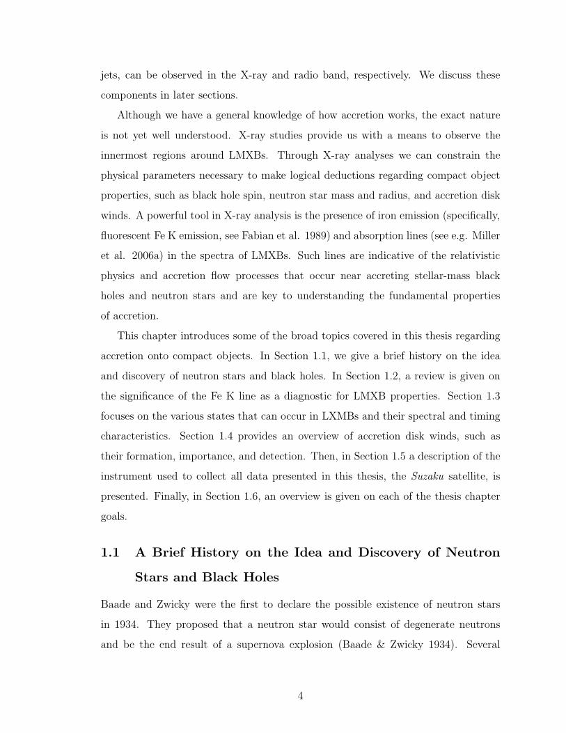
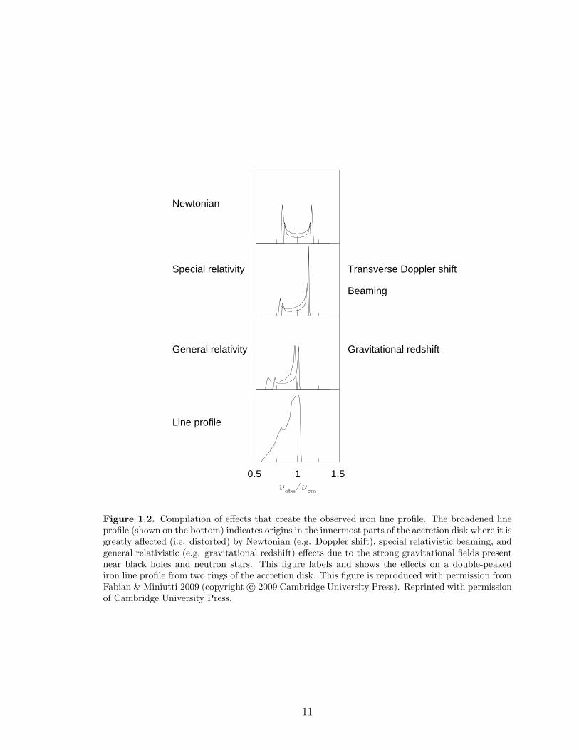
Although the Fe K line is intrinsically narrow, we observe a broadened, (some-

times) asymmetric line profile in the spectra of black hole and neutron star LMXBs.

Indeed, broadened Fe K emission lines have been found in the X-ray spectra in

7

stellar-mass black hole LMXBs (Miller et al. 2002), neutron star LMXBs (e.g. Bhat-

tacharyya & Strohmayer 2007, Cackett et al. 2008), as well as Active Galactic Nuclei

(Nandra et al. 1997, Reynolds 1997). Despite these fluorescent iron lines being

weaker in neutron star LMXBs than in stellar-mass black hole LMXBs, many recent

studies have found them in various neutron star LMXB systems (e.g. D’Ai et al.

2009, 2010; Cackett et al 2008, 2010). The broadened line profile indicates origins in

the innermost parts of the accretion disk where it is greatly affected (i.e. distorted)

by Newtonian (e.g. radial Doppler shift), special relativistic beaming and transverse

Doppler shifts, and general relativistic (e.g. gravitational redshift) effects due to the

strong gravitational fields present near black holes and neutron stars (see Figure 1.2;

e.g. Fabian et al. 2000, Miller 2007 for a review). Thus, the shape of the iron line

profile can be used to constrain the physical properties of compact object, such as

the extent of the inner accretion disk radius.

The Fe K emission line is an important diagnostic of black hole spacetime geometry

and can be used to obtain general constraints on the spin for black holes. Black

holes are frequently described as having “no hair.” That is, only two parameters

are necessary to describe a black hole: mass and spin (assuming the black hole is

electrically neutral, see Blandford & Znajek 1977). As such, knowing the black hole

spin can help to test the predictions of the Kerr metric.

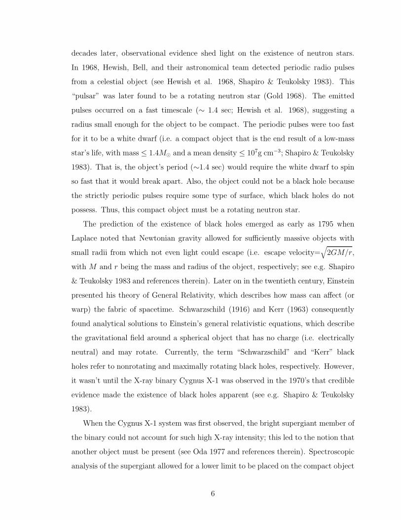
Within the inner disk radius, the circular orbit of inflowing material is no longer

stable and falls quickly into the black hole. Also, there is no viscosity (and thus, no

thermal spectrum) within this radius. This inner boundary is known as the Innermost

Stable Circular Orbit (ISCO). The radius of the ISCO is determined by the spin of

the black hole: rISCO = 6.0 rg for a=0, and rISCO = 1.25 rg for an astrophysical

maximum of a = 0.998 (where rg = GM/c2 with M as the black hole mass, and a =

cJ/GM2, see Figure 1.3; Thorne 1974, and Bardeen, Press, & Teukolsky 1972). The

location of the ISCO determines the “strength” of the gravitational effects on the Fe

K emission line, thereby influencing how broad and skewed the line profile becomes.

Therefore, determining the ISCO through line-fitting serves as an indirect measure

of the black hole spin parameter.

8

Regarding neutron star LMXBs, the Fe K emission line represents an important

method for getting constraints on the nature of ultradense matter present in neutron

stars. As mentioned previously, neutron stars are the densest objects in the Universe

(see e.g. Baym & Pethick 1975). As such, they are an excellent means of studying

dense matter physics. Neutron stars may be composed of strange quark matter,

demonstrate superfluidity (i.e. neutron fluid that flows without any resistance) and

superconductivity (i.e. zero electrical resistance) as well as other phenomena that

cannot be recreated in a laboratory (see Lattimer & Prakash 2004). In order to

understand the structure of neutron stars, it is necessary to know both the neutron

star mass and radius; these physical parameters are essential for determining the

equation of state (EOS) (i.e. composition) of dense matter. Theoretically, multiple

EOS models exist for a given neutron star mass and radius (Lattimer & Prakash

2001). However, it is through X-ray observation that we can get constraints on the

neutron star EOS. The Fe K emission line, for example, can be used to constrain

the radius of the neutron star. Unlike black holes, the inner radius of the accretion

disk around a neutron star must truncate at the star’s surface. Thus, we can use the

iron line to get a lower limit on the inner disk radius and therefore an upper limit on

the neutron star radius (Cackett et al. 2008, 2010). In the case of disk truncation

at the stellar surface, it is assumed that the neutron star is larger than its ISCO.

However, it is quite possible for the neutron star to be smaller than its ISCO. In

this case, obtaining a lower limit on the inner disk radius (assuming that the inner

disk extends to the ISCO) still provides an upper limit on the neutron star radius.

These upper limits provide an important step towards constraining the neutron star

EOS and understanding the behavior of dense matter in extreme environments. We

discuss this further in Chapter 3.

A variety of spectral models exist for fitting the shape of the iron line profile in

order to extract physical parameters such as black hole spin, inner disk radius, orbital

inclination, emissivity (i.e. efficiency of line emission as a function of disk radius),

etc. Each model presented in this work is designed for use with the X-ray Spectral

Fitting Package (XSPEC, Arnaud 1996). We will discuss each model used in detail

9

in later chapters.

1.3 Spectral States

Spectral states are defined to be recurring patterns of spectral and timing character-

istics that a source exhibits (van der Klis 2006). Understanding the nature of spectral

states and the causes of state transitions remains a difficult problem in the study of

LMXBs. State transitions can occur on the order of days to months, and thus can be

observed on human timescales. There have been many conjectures regarding the ori-

gin of state transitions. It is likely that state transitions are at least partially driven

by changes in the mass accretion rate, M , which could potentially cause secondary

changes in parameters such as the inner radius of the accretion disk (see e.g. Esin

et al. 1997, van der Klis 2006). Other physical components that may be involved or

drive state transitions include a corona, a boundary layer (located where the neutron

star surface and accretion disk meet), a magnetosphere, or a jet (van der Klis 2006,

Fender 2006, Lin et al. 2010). Having a greater knowledge of the behavior of these

components can give us insight into the dynamical and kinematic properties that

govern spectral states. While much progress has been made towards understanding

the nature of spectral states, it is still not clear how the above components are in-

volved in state transitions. Each of our subsequent chapters discuss the significance

of spectral states that the observed sources exhibit. Thus, in this section we describe

the various state transitions found in black hole LMXBs and neutron star LMXBs.

Black hole LMXBs can transition between the “quiescent state,” and active states

known as the “low/hard state” (i.e. the low flux hard X-ray state), the “high/soft

state” (i.e. the high flux soft X-ray state), and the “very high state.” When a source

enters one of the active states, it is stated to be in “outburst.”

Outbursts are likely triggered by a thermal disk instability (also known as the

“hydrogen ionization” instability; see e.g. Frank et al. 2002, King 2006). A simple

description of this theory (the nuances of the physics make it more complicated) is

that it predicts that if hydrogen is in a neutral state throughout the accretion disk,

then the source is in a state of quiescence (i.e. no matter is accreted onto the compact

10

0.5 1 1.5

Line profile

Gravitational redshiftGeneral relativity

Transverse Doppler shift

Beaming

Special relativity

Newtonian

Figure 1.2. Compilation of effects that create the observed iron line profile. The broadened lineprofile (shown on the bottom) indicates origins in the innermost parts of the accretion disk where it isgreatly affected (i.e. distorted) by Newtonian (e.g. Doppler shift), special relativistic beaming, andgeneral relativistic (e.g. gravitational redshift) effects due to the strong gravitational fields presentnear black holes and neutron stars. This figure labels and shows the effects on a double-peakediron line profile from two rings of the accretion disk. This figure is reproduced with permission fromFabian & Miniutti 2009 (copyright c© 2009 Cambridge University Press). Reprinted with permissionof Cambridge University Press.

11

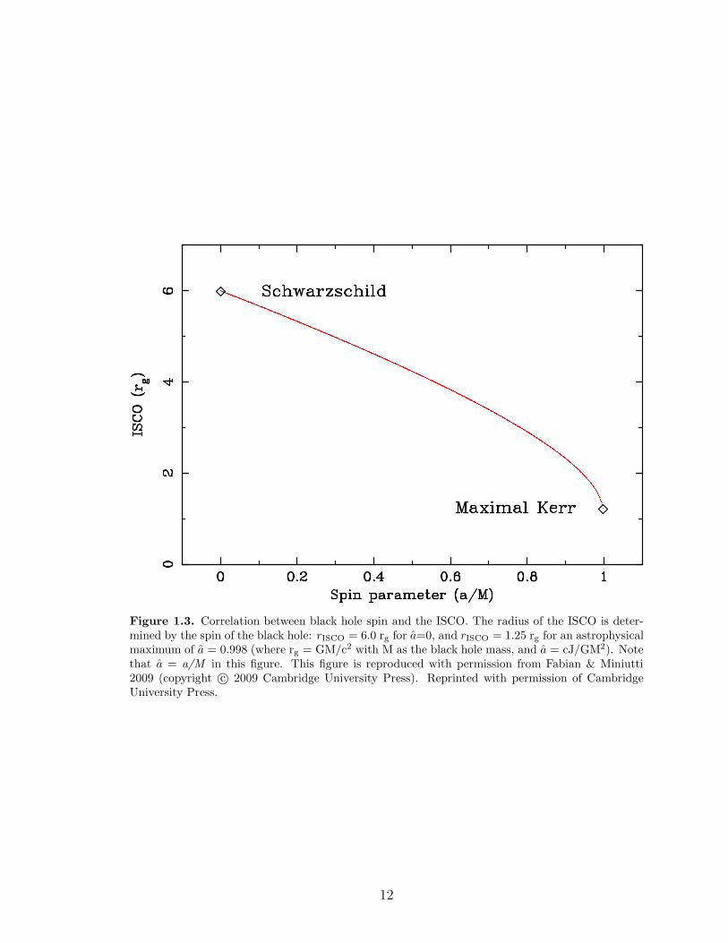
Figure 1.3. Correlation between black hole spin and the ISCO. The radius of the ISCO is deter-mined by the spin of the black hole: rISCO = 6.0 rg for a=0, and rISCO = 1.25 rg for an astrophysicalmaximum of a = 0.998 (where rg = GM/c2 with M as the black hole mass, and a = cJ/GM2). Notethat a = a/M in this figure. This figure is reproduced with permission from Fabian & Miniutti2009 (copyright c© 2009 Cambridge University Press). Reprinted with permission of CambridgeUniversity Press.

12

object and the source is faint). Similarly, if ionized hydrogen exists anywhere within

the disk, the source is in outburst. The surface termperature of the accretion disk

can be raised (in part due to irradiation from an external source) to that of ionized

hydrogen (TH ∼ 6500 K). If this occurs at any radius of the disk, the disk becomes

unstable and an outburst occurs (see e.g. Frank et al. 2002; Figure 1.1, which shows

an LMXB in an active state). When the disk is stable, the source is in quiescence

and material builds up in the outer boundaries of the accretion disk without accreting

onto the compact object.

The disk instability model agrees with the timescales observed in LMXBs. The

relevant timescales for radiatively efficient, geometrically thin (i.e. disk scale height

<< disk radius) accretion disks (see e.g. Shakura & Sunyaev 1973) are the dynamical,

thermal and viscous timescales. These timescales define how the physical structure of

the disk may change. The dynamical timescale is shortest and is related to the orbital

angular velocity (Ω) of the material (tdyn∼Ω−1). The thermal timescale describes how

long it takes energy to be radiated from the disk and is >tdyn. Both the dynamical and

thermal timescales, which are typically on the order of minutes, are much shorter than

the viscous timescale, which is on the order of days to weeks (tdyn<tthermal<<tviscous

see e.g. Frank et al. 2002). Essentially, the viscous timescale defines how long an

outburst lasts since it is the timescale on which angular momentum gets redistributed

within the disk. As mentioned previously, viscosity causes angular momentum to be

transferred outward and thus allows material to accrete onto the compact object.

Orbiting material must lose energy faster than the angular momentum distribution

in order for disk formation to occur (see e.g. Frank et al. 2002). The disk instability

model correctly portays the source alternating between outburst and quiescence on

a thermal timescale and lasting in each of these states on the viscous timescale (see

King 2006 and references therein). In theory, LMXBs that experience this instability

are “transient” while sources where hydrogen is ionized throughout the entire disk

(and thus, the instability is suppressed) are “persistent.”

Thus, LMXBs can be divided into two classes: transient and persistent sources.

Persistent sources can be described as always having a high enough X-ray flux to be

13

detected. Transient sources, on the other hand, experience relatively long periods (i.e.

ranging from months to years) of quiescence (i.e. very faint in the X-ray) interspersed

with short outbursts, where the X-ray luminosity can increase by several orders of

magnitude (see e.g.Psaltis 2006 and references therein). Black hole LMXBs are more

likely to be transients than neutron star LMXBs. This is may be due to weaker disk

irradiation (because black holes do not have a surface) and larger disks (see Frank et

al. 2002).

Luminosity is not always a useful basis for categorizing these active states (e.g.

the low/hard state is not always fainter than the high/soft state; see McClintock &

Remillard 2006 and references therein). For the purpose of this work, we use the

terms “hard,” “soft,” and “steep power-law” to represent the low/hard state, the

high/soft state, and the very high state, respectively. When a typical black hole goes

into outburst, it goes from the hard to soft state before transitioning back (see e.g.

Remillard & McClintock 2006, van der Klis 2006). As the source transitions between

these states it typically passes through the steep power-law state. While some suggest

that the steep power-law state is in itself an “intermediate” state, we acknowledge

the steep power-law state as a bona fide state of black hole binaries in accordance

with McClintock & Remillard (2006).

The quiescent state has the faintest luminosity of all the spectral states (by > 3

orders of magnitude i.e. LX = 1030.5−1033.5ergs−1; see e.g. McClintock & Remillard

2006). It is spectrally defined to be completely nonthermal and hard with a power-law

component and a photon index, Γ, (defined such that constant x E−Γ) of 1.5−2.1.

This state is significant because the faintness of the compact object allows for spectral

and dynamical measurements of the companion star. Such measurements can, for

example, allow for estimates of the mass function, f , and provide absolute lower

limits on the mass of the compact object.

In this work, all observations of the black hole LMXBs were taken when the sources

were in the hard state. The hard state is characterized by an energy spectrum that

is dominated by a power-law-like component (in the 2−20 keV range). As such, disk

reflection spectra (including the Fe K emission line) are more prominent in this state.

14

A photon index of ∼ 1.6 and a high-energy cutoff at ∼ 100 keV (Fender & Belloni

2004) are typical for a black hole X-ray binary in the hard state. A weak soft X-

ray component, most likely associated with a “cool” (i.e. T < 1 keV) thermal disk

(e.g. Miller et al. 2006b, Reis et al. 2009a), can also be present (see Figure 1.4).

According to Nowak (1995), the total X-ray luminosity for systems in the hard state

where distance and mass estimates are known is generally below 10% of the Eddington

luminosity (LEDD = 4πGMmprotonc/σT ≃ 1.3 x 1038 (M/M⊙) erg s−1, where M is

the compact object mass and σT is the Thomson scattering cross-section).

Esin et al. (1997) gave the archetypal model of how accretion flows change with

state. In that model, the inner disk in the hard state is radially truncated at low mass

accretion rates (corresponding to LX/LEDD ≤ 0.008) and an advection-dominated

accretion flow (ADAF; see e.g. Narayan & Li 1994, 1995a,b) is present. That is,

the inner disk is at a larger radius and an ADAF fills the interior. In an ADAF,

energy released in the disk due to viscosity is accreted with the material instead

of being radiated away (this partially explains the typical lower luminosities found

in the quiescent and hard states). However, the notion that radially recessed disks

exist in the hard state may not always be the case (see Chapter 2). Recent analyses

of GX 339-4, Cygnus X-1, SWIFT J1753.5-0127, and XTE J1817-330 have revealed

cool accretion disks that appear to remain close to the black hole at low accretion

rates (Miller et al. 2006b, c, Rykoff et al. 2007, Tomsick et al. 2008). An additional

characteristic of the hard state is the presence of jets, which shall be discussed further

in the next section.

In contrast with the hard state spectrum, a strong thermal component, which can

be modeled as a disk-blackbody with an inner temperature of 1−2 keV, is prevalent

(in the 2−2- keV range) in the soft state (see Figure 1.4; e.g. Fender & Belloni

2004). Although a power-law component is present, the photon index is much steeper

(2.1<Γ<4.8) and is not prominent at hard X-ray energies. Disk reflection spectra are

less typical in the soft state (due to the lack of hard X-ray photons). Moreover, jets

are absent in the soft state, which may lead to potential correlations between disk

winds and jets (see next section).

15

The steep power-law state appears to be a quasi-steady state that shares some of

the characteristics of both the hard and soft states. The energy spectrum possesses

strong thermal and power-law components with no apparent high-energy cutoff (Γ is

typically ≥ 2.4; see Figure 1.4). It is currently unknown whether jets are present in

the steep power-law state (see McClintock & Remillard 2006).

In neutron star low-mass X-ray binaries, a type of spectral state can be inferred

from a source’s location on its X-ray color-color (i.e. soft color vs. hard color) diagram

(CD) (see Chapter 3). Low-magnetic field neutron star LMXBs are categorized into

two types of sources whose names are derived from the patterns that they trace out on

their CD: “Z” sources and “atoll” sources. Z sources tend to be much more luminous

(∼ 0.5−1 Ledd) than atoll sources (∼ 0.01−0.2 Ledd) (van der Klis 2006, Homan et

al. 2010). The atoll source 4U 1636-53 will be the focus of Chapter 3.

The three main spectral states for atoll-type sources are the “extreme island”

(“hard”) state, the “island” (“transitional”) state, and the “banana” (“soft”) state

(see e.g. Jonker et al. 2000 and van Straaten et al. 2003). Note that the “island”

state is spectrally hard compared to the “banana” state. Van der Klis (2006: Fig. 2.4)

portrays these states on the CD of an atoll source. Generally, as a source transitions

from the extreme island state to the banana state, there is thought to be an increase

in mass accretion rate as well as an increase in its variability (i.e. an increase in kHz

quasi-periodic oscillation frequencies: van der Klis 2006).

1.3.1 QPOs and Neutron Star Equation of State

In this thesis we discuss “quasi-periodic oscillations” (QPOs). These frequencies are

present in both black hole and neutron star LMXBs and are very useful for under-

standing the general relativistic effects that occur near the compact object (for a

review, see McClintock & Remillard 2006, van der Klis 2006). We focus mostly on

the kHz QPO frequencies present in neutron star LMXBs (see Chapter 3). In a

power spectrum, two kHz QPO peaks are present (see Figure 1.5). These peaks tend

to shift in frequency (typically in the 200−1200 Hz range) as the source changes

spectral state (see van der Klis 2006). The higher and lower frequencies are called

16

“upper kHz QPOs” and “lower kHz QPOs,” respectively. A current theory is that

upper kHz QPOs represent the Keplerian orbital frequencies at the inner edge of the

accretion disk; the lower kHz QPOs may be the result of the interaction between the

neutron star’s spin frequency and the inner disk orbital frequency (see van der Klis

2006 and references therein). Within this work, we analyze and discuss kHz QPOs

present in neutron star LMXBs and how they can be used in conjunction with Fe K

emission line measurements to estimate the mass of a neutron star.

Our analysis of iron line profiles in a source that exhibits kHz QPOs allows us

to estimate the mass of the neutron star in 4U 1636-53 (see Chapter 3; Piraino et

al. 2000, Cackett et al. 2008). This is an important step towards getting constraints

on the nature of ultra-dense matter. Assuming that the upper kHz QPO frequency

represents the orbital frequency at the inner edge of the accretion disk, we can use

the expression, νorb = (1/2π)√

GM/r3, to get a constraint on the mass. Thus, using

kHz QPO frequencies and the values of the inner disk radius, r (in units of RG), from

Fe K emission line measurements results in an estimate of the neutron star mass and

constraint on the neutron star EOS.

1.4 Disk Winds and Jets

Accretion disk winds, which are inferred from an outflow of ionized gas, can be key to

understanding the nature of the accretion flow in disk systems (e.g. Proga 2003, Ueda

et al. 2009, Ohsuga et al. 2009; Figure 1.1). Typical wind velocities can range from

several hundred to several thousand kilometers per second (v/c < 0.1) (see e.g. Miller

et al. 2006a, Neilsen & Lee 2009). The physical mechanism needed to produce such a

disk wind is still being investigated, aided by an extensive theoretical framework; pos-

sibilities include thermally driven, radiation driven, and magnetically driven winds

that originate from the accretion disk (see e.g. Blandford & Payne 1982, Begelman

et al. 1983, Proga et al. 1998, 2000). Each possibility involves a different physical

process for creating disk winds; therefore, each can provide significant information

about the fundamental properties of the accretion disk itself, such as the disk’s ion-

ization, temperature, mass accretion rate, geometry, and magnetic field (assuming a

17

Steep power-law

Soft

Hard

Figure 1.4. Black hole LMXB spectral states. In order from top to bottom, the steep power-law state, soft state, and hard state are labeled. The black data points show the overall energyspectrum. The red line, blue dashed line, and black dotted line represent the thermal component,power-law component, and reflection component, respectively. Note which components dominantfor each spectral state. For example, the hard state has a strong power-law component while the softstate has a prevalent thermal component. Meanwhile, the steep power-law state possesses strongthermal and power-law components. This figure is reproduced with permission from Remillard &McClintock 2006.

18

Figure 1.5. Two kHz QPO peaks in a power spectrum. This figure shows an example of the kHzQPOs present in neutron star LMXBs (specifically, the source Scorpius X-1). The higher and lowerfrequencies are called “upper kHz QPOs” and “lower kHz QPOs,” respectively. Upper kHz QPOsmay represent the Keplerian orbital frequencies at the inner edge of the accretion disk; the lowerkHz QPOs may be the result of the interaction between the neutron star’s spin frequency and theinner disk orbital frequency (see van der Klis 2006 and references therein). This figure is reproducedwith permission from van der Klis et al. 1997, 2006.

19

!"##$%#&'"()$

*"+,-#$%./)$

Figure 1.6. Neutron star equation of state. This figure shows the multiple possibilities for theequation of state (EOS) of a neutron star (EOS labels are as defined in Lattimer & Prakash 2001).Both radius and mass are the crucial parameters to get a constraint on the neutron star EOS. Thisfigure is adapted with permission from Lattimer & Prakash 2001. Reproduced by permission of theAAS.

20

magnetic field is “threaded” throughout the disk). Evidence of disk winds can be

found through X-ray spectral absorption lines, which are Doppler-shifted. Material

in the wind (i.e. the ionized gas) absorbs radiation emitted by the central engine and

produces absorption lines along our line of sight. These lines are also blue shifted

(i.e. Doppler shifted to higher energies) because the material is coming towards us.

In Chapter 4, we discuss whether disk winds are present in the black hole LMXB

H1743-322 through a search for ionized iron absorption lines, specifically Fe XXV

(6.70 keV) and Fe XXVI (6.97 keV), while the source was in the hard state. An

interesting aspect of disk winds is that they are not present in every spectral state.

Indeed, they appear to “turn off/on” depending on spectral state, indicating that an

innate feature of the accretion disk is changing.

Compared to disk winds, jets are collimated (see Figure 1.1), relativistic outflows

characteristically observed in (but not limited to) the radio band. Observationally,

radio images of jets have been resolved in a number of binaries, including the black

hole LMXB GRS 1915+105 (Mirabel & Rodrıguez 1994, Fender et al. 1999). Some

sources, such as GRS 1915+105, have highly relativistic jets (v/c ≥ 0.9) that show

apparent superluminal motion. Jets are assumed to be a ubiquitous feature of LMXBs

and, as such, represent a connection with other accreting compact objects (see Fender

2006). These powerful outflows emit radio waves most likely due to a process known as

“synchrotron emission” (electromagnetic radiation that is produced when relativistic

particles are accelerated along magnetic field lines). That is, the non-thermal spectra

and polarized radiation observed in jets are consistent with what is expected from

synchrotron emission. Although jets show energy and matter being carried away

from the binary system, the jet composition (aside from charged particles such as

electrons and positrons) is not well known; observing spectral emission lines in jets is

extremely rare (see Fender et al. 2006 and references therein). Regarding the origin

of jet formation, it is theoretically possible that spin energy from a black hole can

partially contribute to powering jets in black hole LMXBs (Blandford & Zjanek 1977).

However, multiple hypotheses exist that use the idea of magnetic fields “threaded”

throughout the accretion disk powering the jets (see e.g. Blandford & Payne 1982).

21

Thus, there would be a correlation between the jets and the accretion disk.

In LMXBs, there is a potential connection between disk winds and jets, which are

relativistic outflows most prominent in the radio-band. Disk-jet coupling, i.e., the

relation between inflow and outflow, is extremely important in X-ray binary research.

The hard and the soft states are the two most diametrically opposed in regards to jet

formation. For example, when both GRS 1915+105 (Dhawan et al. 2000) and Cyg

X-1 (Stirling et al. 2001) were in the hard state, Very Long Baseline Interferometry

(VLBI) radio images have shown a spatially-resolved radio jet during periods of quasi-

steady radio and hard X-ray emission. However, in the soft state there is a dramatic

drop in the radio emission compared to the hard state (e.g. Fender & Belloni 2004).

Although the nature of radio emission in the steep power-law state remains unclear,

McClintock & Remillard (2006) suggest that this state is relatively radio quiet. To

date, no source has exhibited optically-thick radio emission consistent with a jet in

the soft state. Our research efforts in Chapter 4 may give further evidence to the

possibility of a spectrally state-dependent anti-correlation between winds and jets.

That is, when disk winds are present, jets are absent and vice versa. This potential

connection may offer insights into the nature of the spectral states. In this work we

discuss disk winds and jets solely in the context of black hole LMXBs (for a review

of disk-jet coupling in both neutron star and black hole LMXBs, see Fender 2006).

However, it is interesting to note that in the context of disk-jet coupling, X-ray flux

and radio flux (assuming emission from the accretion disk and jets, respectively)

correlations exist for both black hole and neutron star LMXBs in the hard state

(Migliari & Fender 2006). This may indicate that connections between jets and the

accretion disk depend on the fundamental properties of the accretion flow and not

the type of compact object (Migliari & Fender 2006).

1.5 The Suzaku X-ray Satellite

The primary telescope used to collect the data presented in this work is the Suzaku

X-ray satellite (see Figure 1.7). Suzaku is a joint Japanese-U.S. mission that was

launched on July 10, 2005. At a weight of approximately 1600 kg, the Suzaku space-

22

craft has a circular, 96 minute orbit around Earth at an altitude of 550 km (Mitsuda

et al. 2007). One of the major instruments on board Suzaku is the X-ray Imaging

Spectrometer (XIS, Koyama et al. 2007; see Figure 1.8), which detects “soft” X-rays

(i.e. 0.2−10 keV) and consists of four units (XIS0, XIS1, XIS2, XIS3) that are each

an X-ray CCD camera (CCD: Charge-Coupled Devices, similar to CCDs used in dig-

ital cameras; Koyama et al. 2007). CCDs have become essential observational tools

in the field of X-ray astronomy because they provide accurate energy measurements.

The CCD cameras on Suzaku each consist of one silicon CCD chip that is sensitive

to X-rays and is 25 mm x 25 mm in size (Koyama et al. 2007, Mitsuda et al. 2007).

Each XIS unit provides images that cover 18 arcminutes x 18 arcminutes of the sky

(Koyama et al. 2007, Mitsuda et al. 2007). When an incoming X-ray photon hits a

pixel on the CCD (i.e. an “event” occurs), it gets converted into an electric charge

that produces a voltage at the output of the CCD. This voltage is proportional to

the energy of the incident photon. Thus, the resulting measurement is an accurate

estimate of the original X-ray photon’s energy.

The Suzaku XIS cameras provide the spectral resolution necessary for relativistic

line detection, such as the Fe K emission line. At 6 keV for example, XIS has an

energy resolution of ∼ 130 eV ( or an E/δE of ∼ 50; Koyama et al. 2007). This

resolution makes it easier to determine the actual shape of the line profile, which is

essential for constraining the physical properties of LMXB systems (see e.g. Miller

et al. 2010).

Within this work we use the XIS0, XIS1, and XIS3 cameras for the sources pre-

sented in subsequent chapters. Note that XIS2 was irreparably damaged in November

2006 (prior to all of our observations) and no data from it could be used (Koyama

et al. 2007; SUZAKU-MEMO-2007-08). The 2x2, 3x3 and 5x5 observation editing

modes are used, which were chosen based on the counting rate and the telemetry

limit (see Koyama et al. 2007). The number of the modes indicates the number of

pixels centered on the event (e.g. 5x5 mode means that pulse heights of 25 pixels

are received; thus this mode contains the most detailed information). Additionally,

a “window/burst” option was used for each of our observations in order to decrease

23

the effective area of the CCD (only a fraction of the CCD is read out at a time)

and therefore, shorten the exposure times. This is necessary when observing bright

sources because it reduces the effects of photon pile-up, which occurs when multiple

photons get mistakenly registered as one event. This, for example, would lead two

low energy X-ray photons to be registered as one high energy X-ray photon and cause

false representation of the continuum and relativistic lines (Miller et al. 2010).

The second major instrument on board Suzaku is the Hard X-ray Detector (HXD,

Takahashi et al. 2007; see Figure 1.8), which is highly sensitive and can detect “hard”

X-rays (i.e. X-rays of higher energy) in the 10−600 keV energy range and has a field

of view of 34 arcmin x 34 arcmin (≤ 100 keV) and 4.5 x 4.5 (≥ 100 keV) (Takahashi

et al. 2007, Kokubun et al. 2007, Mitsuda et al. 2007). Unlike the XIS, the HXD

is a collimated, non-imaging, hard X-ray detector. The two main types of detectors

within each of the 16 main HXD units are the Gadolinium Silicate (GSO) phoswich

counters, or scintillators, (composed of crystals that fluoresce when hit with high

energy photons) and the Positive Intrinsic Negative (PIN) silicon diodes (Takahashi

et al. 2007, Kokubun et al. 2007). The HXD/PIN and HXD/GSO cameras are

sensitive between ∼ 10−70 keV and 40−600 keV, respectively, and have an energy

resolution (FWHM) of about 4 keV and 7.6/√

EMeV % (where E is energy in MeV),

respectively (Takahashi et al. 2007, Kokubun et al. 2007).

Each of the 16 main HXD detectors are of “well-type” design (Takahashi et al.

2007). X-rays that make it “all the way down the well” come from the direction of

interest (i.e. the object at which the HXD is pointed) and are therefore “collimated.”

This collimation allows for high sensitivity (i.e. the ability to detect dim object).

The PIN diodes are located above the GSO scintillators within the “well”; photons

below ∼ 70 keV are photoelectrically absorbed by these diodes and the corresponding

energies recorded digitally (Takahashi et al. 2007, Kokubun et al. 2007). X-rays

of higher energy, however, pass through the PIN diodes and are recorded by the

photomultiplier tubes connected to the GSO scintillators (Takahashi et al. 2007,

Kokubun et al. 2007). Thus, the high sensitivity and large energy bandpass provided

by the Suzaku HXD allows for more accurate modeling of the continuum as well as

24

Figure 1.7. Artist rendition of Suzaku. Courtesy of JAXA.

the reflection spectrum.

1.6 Thesis Overview

In this thesis we explore the nature of three accreting X-ray binaries using spectral

analysis. Specifically, we analyze Suzaku spectra from two stellar-mass black hole

LMXBs, GRS 1915+105 and H1743-322, and one neutron star LMXB, 4U 1636-53.

All spectra were fit using the X-ray spectral fitting package (XSPEC, Arnaud 1996);

every spectral model we employed was designed to be used in this package. We discuss

these spectral models in more detail in subsequent chapters. Each binary system will

be the focus of one chapter in which we present our findings and discuss them in

the larger context of compact object properties such as black hole spin, neutron star

mass and radius, and accretion disk winds.

25

Figure 1.8. Internal schematic of Suzaku. The two major instruments: theX-ray Imaging Spec-trometer (XIS) and the Hard X-ray Detector (HXD) are labeled. Note how each XIS unit is atthe focus of an X-ray Telescope (XRT). This figure is adapted with permission from Mitsuda et al.2007.

26

1.6.1 Black Hole Spin

Chapter 2 discusses the black hole spin of GRS 1915+105, which harbors one of the

most massive known stellar black holes in the Galaxy. Fits to the spectra with simple

models reveal strong disk reflection through an Fe K emission line and a Compton

back-scattering hump. We report constraints on the spin parameter of the black hole

in GRS 1915+105 using relativistic disk reflection models. The model for the soft

X-ray spectrum (i.e.< 10 keV) suggests a = 0.56+0.02−0.02 and excludes zero spin at the 4σ

level of confidence. The model for the full broadband spectrum suggests that the spin

may be higher, a = 0.98+0.01−0.01 (1σ confidence), and again excludes zero spin at the 2σ

level of confidence. We discuss these results in the context of other spin constraints

and inner disk studies in GRS 1915+105.

1.6.2 Inner Disk Radius and Neutron Star Radius

In Chapter 3 we present an analysis of 4U 1636-53, which reveal the presence of

broad iron line profiles. These Fe K lines are well fit by a model for lines from a

relativistic accretion disk (diskline), permitting a measurement of the inner radius

of the accretion disk and therefore an upper limit on the neutron star radius. We find

that the inner disk radius, as measured by the iron line profile and disk continuum,

does not change significantly in our observations when the source is in the island

(transitional) state and the medium-luminosity banana (soft) state, suggesting that

the inner disk radius may not vary with these states. The simultaneous presence of

kHz QPOs rules out dense wind outflows as the source of broadening. The iron line

and kHz QPO measurements together permit a mass constraint of M≤ 2.4M⊙.

1.6.3 Disk Winds and Jets

Chapter 4 addresses the absence of disk winds in H1743-322 while the source was

in a hard state during its 2008 outburst. Fits to the spectra with simple models

fail to detect narrow Fe XXV and Fe XXVI absorption lines, with 90% confidence

upper limits of 3.5 eV and 2.5 eV on the equivalent width, respectively. These limits

are commensurate with those in the steep power-law state, but are well below the

27

equivalent widths of lines detected in the soft state, suggesting that disk winds are

partially state-dependent. We discuss these results in the context of previous detec-

tions of ionized Fe absorption lines in H1743-322 and connections to winds and jets

in accreting systems. Additionally, we report the possible detection of disk reflection

features, including an Fe K emission line.

1.6.4 Conclusions

In Chapter 5 we summarize our results and discuss our findings in the broader context

of the fundamental properties of accreting compact objects.

28

CHAPTER 2

Measuring the Spin of GRS 1915+105 with

Relativistic Disk Reflection

2.1 Introduction

GRS 1915+105 was discovered by the WATCH instrument on board the Granat

satellite on 1992 August 15 (Castro-Tirado et al. 1992) . It has since been classified

as a microquasar: a Galactic jet source with properties similar to quasars, but on a

stellar scale. The mass of the central compact object is estimated to be 14±4 M⊙

(Greiner et al. 2001). The authors reported results on the optical counterpart that

implied a K-M III donating star of ∼ 1.2 M⊙, making GRS 1915+105 a low-mass X-

ray binary. GRS 1915+105 is well-known for its extreme variability across all bands of

the electromagnetic spectrum (Belloni et al. 2000). Additionally, in 1998, BeppoSAX

observations of GRS 1915+105 showed the clear presence of a broad emission line at

6.4 keV (Martocchia et al. 2002), i.e. the Fe Kα line.

In our modeling of the X-ray spectrum, we make the assumption that the accretion

disk extends down to the innermost stable circular orbit (ISCO) in the hard state.

The luminosity observed in GRS 1915+105 (L ∼ 0.30 LEDD) is higher than what is

theoretically calculated for a truncated disk in the hard state (Esin et al. 2007). This

higher luminosity, and therefore higher mass accretion rate, is indicative of inner disk

extending closer to the black hole (e.g. Esin et al. 2007: Fig. 1) and supports the

notion that truncated disks in the hard state may not always be the case (see e.g.

Miller et al. 2006b, c, Rykoff et al. 2007, Tomsick et al. 2008).

Spectral fits to thermal emission from the accretion disk in black hole binaries

provides an independent way to constrain black hole spin. In order to turn the flux

29

observed from the disk continuum into a radius (and therefore a spin parameter), the

source distance, inclination, and mass must be known. In addition, factors like the

line of sight absorption, hardening due to scattering in the disk atmosphere, and the

form of the hard spectral component can be important. In order to obtain reliable

spin estimates using the continuum method, it is crucial for the source to have a

strong thermal component (e.g. McClintock & Remillard 2009). For the case of GRS

1915+105, this thermal component is most easily observed while in the soft state.

However, prior spin results that have been reported for GRS 1915+105 in this state

are not consistent. McClintock et al. (2006) and Middleton et al. (2006) both used

models for thermal continuum emission from the accretion disk to calculate values

of a >0.98 and 0.72+0.01−0.02, respectively. In this chapter, we present an independent

analysis using the relativistic disk reflection spectrum to calculate the black hole spin

in GRS 1915+105 in the hard state with the advanced cameras on Suzaku.

2.2 Data Reduction

Suzaku observed GRS 1915+105 on 2007 May 7 starting at 14:40:22 (TT). The obser-

vation duration was approximately 117 ks. The XIS pointing position was used. In

order to prevent photon pileup, the XIS cameras were operated using the 1/4 window

mode using a 1.0 s burst option. The XIS1 and HXD/PIN cameras were used in this

analysis. Two other XIS units were turned off to preserve telemetry and the fourth

unit was run in a special timing mode (which has yet to be calibrated). XIS on-source

times of approximately 51 ks were achieved. This resulted in a dead-time corrected

net exposure of 25 ks for the XIS1 camera (in 3x3 editing mode). A net exposure

time of 57 ks was achieved using the HXD/PIN.

For the soft x-ray data, the 2.3−10 keV energy range was used in order to avoid

calibration problems near the Si K edge and because there are few photons at low

energy owing to high line of sight absorption (nH ∼ 4.0 x 1022cm−2). Using the clean

event file (3 x 3 mode data) with the latest calibration databases at the time from the

XIS data (CALDB 20070731: version 2.0.6.13), we extracted the source light curve

and spectrum with xselect. An annulus centered on the source with an inner radius

30

of 78′′ and an outer radius of 208′′ (75 and 200 in pixel units, respectively) was used

for the source extraction region because the center of the image suffered pile-up. An

annulus centered on the source was also used for the background extraction region

with an inner radius of 208′′ and an outer radius of 271′′ (200 and 260 in pixel units,

respectively). We manually corrected for extracted region areas that did not land on

the XIS chip. The XIS redistribution matrix files (RMFs) and ancillary response files

(ARFs) were created using the tools xisrmfgen and xissimarfgen available in the

HEASOFT version 6.6.2 data reduction package. The 3 x 3 mode event file was used

to specify good time intervals and the data was grouped to a minimum of 25 counts

per bin using the FTOOL grppha.

For the HXD data, the latest calibration databases (CALDB 20070710) were

used and the reduction process began with a clean event file from the PIN detector

(energy range 10.0−70.0 keV), which was at XIS aimpoint. In the PIN data reduction

process, the PIN spectrum was extracted and deadtime was corrected by using the

pseudo-events files. After the non-X-ray (NXB) background spectrum was extracted,

the exposure time of the background spectrum was increased by a factor of 10 since

the NXB event file was calculated with a count rate 10 times higher than the real

background count rate to reduce statistical errors. The cosmic X-ray background

was simulated, modeled and added to the NXB spectrum in XSPEC version 12.5.0

as instructed in the Suzaku ABC guide.

2.3 Data Analysis and Results

Using the X-ray spectral fitting software package (XSPEC v. 12.5.0, Arnaud 1996),

we initially fit the Suzaku XIS spectrum of GRS 1915+105 with a simple absorbed

power law model: phabs*(powerlaw), with the phabs model component accounting

for Galactic photoelectric absorption. All parameters were allowed to vary. The

4.0−7.0 keV range was ignored when fitting the data to obtain an unbiased view of

the Fe K range. The fit resulted in an equivalent hydrogen column, nH, of 4.51+0.06−0.06

(in units of 1022cm−2) and a photon index, Γ, of 2.09+0.01−0.01 (χ2/ν = 1402/1282). That

ignored energy range was then restored when forming the data/model ratio as shown

31

in Figure 2.1. An asymmetric, skewed line is revealed in the exact way predicted for

relativistic disk lines. In a similar manner, Figure 2.2 shows the XIS and HXD spectra

fit with a simple model consisting of a broken power-law modified by interstellar

absorption: phabs*(bknpow). A constant was allowed to float between the two data

sets. The 4.0−7.0 keV and 15.0−45.0 keV ranges were ignored when fitting in order

to properly model the continuum. Note that for the HXD spectra, the model was

fit over the 12.0−15.0 keV and 45.0−55.0 keV energy ranges. The fit resulted in nH

= 4.35+0.06−0.07, Γ1 = 2.03+0.02

−0.02, and Γ2 = 2.59+0.02−0.02 with an energy break at 7.7+0.2

−0.2 keV

(χ2/ν = 1565/1312). Again, the ignored energy ranges were restored when forming

the data/model ratio. Note that the residuals near 12 keV can be attributed to

calibration problems near the edge of the detector.

XSPEC provides a number of models for spectral line fitting. Models of particular

interest to us not only allow for analysis of the observed broad iron line in our data,

but account for the special and GR effects that physically go into creating such an

emission profile around a black hole. Since determining the black hole spin of GRS

1915+105 through analysis of the iron line is our main priority, models that allow

spin to be a free parameter in our fits are useful. Brenneman & Reynolds (2006)

have calculated models (kerrdisk and kerrconv) that describe line emission from

an accretion disk and include black hole spin as a free parameter, thereby allowing

us to formally constrain the angular momentum of the black hole and other physical

parameters of the system. The kerrdisk model describes line emission from an

accretion disk, while the kerrconv model allows one to convolve a reflection spectrum

with the smeared line function.

Although general relativity permits the spin parameter a to have any arbitrary

value, black holes can in principle have spin parameters -1 ≤ a ≤ 1. However, for

simplicity the kerrdisk model only considers a black hole that has a prograde spin

relative to the accretion disk that spins up to the Thorne (1974) spin-equilibrium

limit, i.e., 0 ≤ a ≤ 0.998.

In addition to the spin parameter, we can specify and/or constrain nine other

physical parameters in the kerrdisk model: (1) rest frame energy of the line, (2)

32

emissivity index within a specified radius, (3) emissivity index at radii larger than a

specified value, (4) break radius separating the inner and outer portions of the disk (in

units of gravitational radii), (5) the disk inclination angle to the line of sight, (6) the

inner radius of the disk in units of the radius of marginal stability (rms), (7) the outer

radius under consideration, (8) the cosmological redshift of the source (z=0 for our

source), and (9) the normalization (flux) of the line in photons cm−2 s−1. kerrconv

has the same basic set of parameters with the exception that it does not require an

input line energy or a flux normalization parameter since it uses a kerrdisk kernel

to smear the entire spectrum with relativistic effects. Of these parameters, we let 1,

2, 3, 5, and 9 vary freely. We bounded the rest frame energy for the iron line between

6.4 and 6.97 keV and the disk inclination between 55 and 75 based on the figure

presented in Fender et al. (1999: Fig. 6) from radio jet observations. The emissivity

indices were fixed to be equal to each other meaning that we only consider one index,

making the break radius meaningless. Parameters 4, 6 and 7 were frozen at 6.0 rg,

1.0 rms, and 400 rms, respectively using the “standard” values of the kerrdisk and

kerrconv models. By doing this, we assume that the ionization of the disk material

within the ISCO is too high to produce significant line emission as has been shown

by 3D MHD simulations (Reynolds & Fabian 2008).

Our model is defined as: phabs*(kerrdisk+kerrconv*pexriv) (Figure 2.3). A

constant was allowed to float between the XIS and HXD data sets. The model

component pexriv is an exponentially cut-off power-law spectrum reflected from

ionized material (Magdziarz & Zdziarski 1995). The free parameters are the power-

law photon index Γ, the fold energy or cutoff energy (in keV), and the scaling factor

for reflection. Our results are given in Table 2.1 with the model being fit in the

2.3−10.0 keV and 12.0−55.0 keV energy ranges. Note that the residual feature at

the upper limit of the XIS detector is the result of noise. Errors were calculated

using the steppar command in XSPEC, which affords control over how the χ2 space

is searched. For all parameters, errors refer to the 68% confidence level (∆χ2= 1)

unless otherwise stated. The reduced χ2 of our best-fit is 2345/2224. We measure a

spin value of a = 0.98+0.01−0.01. Figure 2.4 plots the dependence of χ2 on the black hole

33

spin parameter. A spin of zero is excluded at the 2σ level of confidence.

The disk ionization parameter (ξ = LX/nr2, where n is the hydrogen number

density) has a large effect on the resulting spectrum. Ross et al. (1999) demonstrated

the effect on reflection spectra models for a range of ionization values ( 30< ξ < 105).

The model with the highest ionization parameter, ξ = 105 was the best reflector but

had negligible iron spectral features due to the disk surface layer being fully ionized

at great depth, with the iron line (specifically, Fe XXVI) not becoming dominant

until τ ≈ 8. However, when ξ is reduced to 3 x 103, less than half of the iron is

fully ionized at the disk’s surface and Fe XXV becomes dominant at τ ≈ 1. Most

importantly, at this value an iron emission line that is Compton-broadened becomes

visible (Ross et al. 1999: Fig 2). Similar to this ionization value is our value of

5000, which is the upper limit allowed by the pexriv model. This “high” value was

chosen so as to obtain the maximum amount of broadening due to Comptonization

and further understand the dynamics of the system. In our model, maximizing or

minimizing the disk temperature (106 and 104 Kelvin, respectively) changed χ2 by

less than 5, resulting in similar reduced χ2 to the best-fit value (χ2/ν ∼ 1.05). Effects

to the parameter values (most notably the spin parameter) were negligible with the

exception of the reflection scaling factor, which changed by < 0.06. Note that a

thermal disk component is not required for our model and, since the disk itself is

likely to be relatively cool and the high Galactic photoelectric absorption prevents its

detection, we have set a low disk temperature (see, e.g., Miller et al. 2006b, Rykoff

et al. 2007).

Given the complexity of the source and it’s extreme variability, we had set the

iron abundance equal to the solar value to provide a more simplistic approach to

constraining the spin, our main parameter of interest. Using the upper limit on the

ionization value we tested the effects of altering the iron abundance in the pexriv

model. Ross & Fabian (2005: Fig. 5) show that increasing the iron abundance

relative to the solar value serves to lower the continuum while enhancing the Fe

Kα emission lines. Additionally, Lee et al. (2002) measured an iron abundance,

Fe/solar, > 1.0 for GRS 1915+105, conveying that the overabundance may be due

34

to dynamics of supernova in the microquasar’s history. However, Ueda et al. (2009)

were more definitive in fitting a spectrum with better statistics using solar values

for the abundances (including iron). As such, after testing the effects of varying

abundance, our pexriv model did not require an enhanced abundance (e.g. tripling

the iron abundance increased χ2 by ∼ 100).

Our broadband model uses pexriv as its main reflection component. One diffi-

culty with this model is that it does not include the effects of Comptonization on

photoelectric absorption edges in the outer, most highly ionized layers of the disk.

Being statistically inferior in this regime, it may not be ideal to use this model for

high values of ξ, which is the reason our value of 5000 erg cm/s is the upper limit.

In order to check how our spin constraints might depend on the reflection model,

we replaced pexriv with a newer, more self-consistent reflection model: reflionx

(see Fig. 2.5). The reflionx model is a revised version of reflion (Ross & Fabian

2005) that describes reflection from accretion disks in black hole systems where the

blackbody emission is at too low an energy to affect the Fe Kα emission. It has been

used previously to constrain the spin in other sources such as GX 339-4 (Reis et al.

2008). The parameters of the model are the iron abundance (set to solar), photon

index of the illuminating power law, ionization parameter, ξ, and the normalization.

In fitting reflionx, the HXD spectrum was neglected because a cut-off power-law is

required whereas reflionx assumes that a simple power-law spectrum irradiates the

disk. Moreover, reflionx is a pure reflection model that requires a simple power-law

to represent the continuum. Note that the Fe K emission line is self-consistently mod-

eled within the reflionx model. Also, in order to obtain better constraints within

the reflionx model, the inclination was bounded between at 55 and 75 . The

model was fit in the 2.3−10.0 keV energy range. Letting a be a free parameter, the

phabs*(powerlaw+kerrconv*reflionx) model resulted in a spin parameter of 0.56

with a χ2 value of approximately 2124 and a reduced χ2 ∼ 1.01 for 2100 degrees of

freedom (see Table 2.2). Based on these results from the reflionx model, we can

state that a = 0.56+0.02−0.02 is preferred and that a spin of zero is excluded at the 4σ level

of confidence (see Fig. 2.6). However, it is important to note that the parameter

35

values obtained with the reflionx model are poorly constrained, which requires the

pexriv results to be viewed with extra caution (see Sect. 4).

Finally, we note the possible presence of an absorption line at approximately

7.4 keV (see Figure 2.1). It is not clear that the feature is real. When the broadband

spectrum is fit phenomenologically, a Gaussian model for the line suggests a (single-

trial) significance of 4σ. The feature is not significant after fitting the relativistic

emission line and disk reflection continuum. If the line is real, it could plausibly be

associated with Fe XXV or Fe XXVI, implying a wind with a blue-shift as high as

0.1c. When a strong line is frozen as part of the overall spectral model, even modest

constraints on the spin parameter of the black hole cannot be obtained. However, a

wind in a hard state would be inconsistent with an apparent anti-correlation between

winds and jets in GRS 1915+105 (Miller et al. 2008a, Nielsen & Lee 2009).

2.4 Discussion

In this chapter, we have presented the first results from Suzaku observations of GRS

1915+105 in a hard state. We have observed the Fe K emission line in GRS 1915+105

in unprecedented detail due to the spectral resolution and fast readout modes of the

XIS cameras. Our broadband spectral model suggests a spin of a = 0.98+0.01−0.01, though

a value of zero is only excluded at the 2σ level of confidence. A different model, fitted

only to the soft X-ray spectrum, results in a spin of a = 0.56+0.02−0.02 with a value of zero

excluded at 4σ level of confidence. This effort to measure the spin of the black hole

in GRS 1915+105 follows other recent efforts to measure spin in stellar-mass black

holes using relativistic iron lines (Miller et al. 2008b, Reis et al. 2008/2009b, Miller

et al. 2009) and the thermal disk continuum spectrum (e.g. Shafee et al. 2006).

Owing to its extreme behavior and the possibility of a relation to the spin of the

black hole, it is particularly important to understand the black hole in GRS 1915+105.

Middleton et al. (2006) and McClintock et al. (2006) used similar thermal emission

continuum models based on different data selections from RXTE to estimate the spin

of the black hole in GRS 1915+105. Middleton et al. (2006) determined the spin of

GRS 1915+105 from a set of 16 RXTE observations (approximately spanning 1994

36

to 1996) that were 16 s each. The authors chose spectra where there was a slow

change between spectral states, specifically variability classes β and λ (Belloni et al.

2000), which is why short time-scale spectral binning was used. They required that

Comptonization contribute less than 15 % of the bolometric flux (or rather that the

disk contributed greater than 85 %). Also, the rms variability had to be < 5 %. For

the final analysis, there were a total of 34 disk dominated spectra for 6 observations.

The XSPEC models used were for a multicolor disk blackbody (diskbb), relativistic

effects (bhspec), and thermal Comptonization (thcomp) that result in an intermediate

spin value of a = 0.72+0.01−0.02

For comparison, McClintock et al. (2006) used a much larger sample of RXTE

data than Middleton et al. (2006) with a total observation time of 89 ks for RXTE

and 13 ks for ASCA. The 22 observations selected had to meet 3 criteria: (1) weak

QPOs, (2) rms continuum power < 0.075 rms, and a (3) disk flux > 75 % of the

total 2-20 keV emission. The authors used a relativistic disk model (kerrbb2: a

combination of kerrbb and bhspec that included a spectral hardening factor), which

would alternately be combined with a power-law, Comptonization (comptt), and a

cut-off power-law model (cutoffpl). These last 3 models represented the nonthermal

tail component of the emission. They argued that the spin (a > 0.98) and mass

accretion rate parameters were relatively unaffected by the model for the nonthermal

tail component.

Both sets of authors have identified several reasons that might explain the dif-

ferent spin values that they derived. McClintock et al. (2006) note the existence of

uncertainties in disk structure at high luminosities. These uncertainties could pos-

sibly affect the Middleton et al. (2006) results, which used solely high luminosity

observations (L > 0.3 LEDD). McClintock et al. (2006) also suggest that Middleton

et al. (2006) missed crucial low luminosity observations because of small data samples

– the derived intermediate spin value may be due to averaging over a wide range of

luminosities (including a super-Eddington luminosity of L ∼ 1.45 LEDD). However,

Middleton et al. (2006) suggest that the McClintock et al. (2006) low luminosity

data (L < 0.3 LEDD) does not allow for a low temperature Comptonized component

37

(kTe < 3 keV).

In summary, McClintock et al. (2006) finds a rapidly spinning black hole in GRS

1915+105 based on disk continuum fits from RXTE and ASCA data. Middleton et al.

2006) used similar assumptions (i.e. d ∼ 12 kpc and inclination angle ∼ 66 (Fender

et al. 1999)) and models, but had a smaller sample of RXTE data of GRS 1915+105

and got an intermediate value of a = 0.72+0.01−0.02. The behavior of GRS 1915+105

is particularly complex and the states identified in this source are more numerous

and nuanced than those identified in other black hole binaries. The differences in

Middleton et al. (2006) can be partly attributed to the state classifications (i.e.

A, B, C) for GRS 1915+105 as opposed to the black hole binary categories used by

McClintock et al. (2006). The spin estimate reported by McClintock et al. (2006) was

obtained in a state that resembles the “thermal state” (i.e. soft state or “thermal

dominant” state). Here, our observation was obtained in the hard state (which is

mostly likely “state C”).

Previous work has suggested that for non-spinning black holes, the amount of Fe K

emission from within the ISCO is negligible: inside the ISCO, the ionization fraction

sufficiently increases close to the black hole making it unlikely that there is significant

Fe K emission within the ISCO since the ionization fraction substantially increases

(Reynolds & Begelman 1997). Reynolds & Fabian (2008) find that systematic errors

on the spin due to emission from within the ISCO become smaller for more rapidly

rotating black holes. Additionally, Shafee et al. (2008) determined that magnetic

coupling is unimportant across the ISCO for geometrically thin disks. The best

current theoretical works suggests that systematic errors are unlikely to bias our

results for GRS 1915+105 (Reynolds & Fabian 2008).

An r−3 disk emissivity relation is typically assumed for line emission from a stan-

dard thin accretion disk with an isotropic source of disk irradiation (see, e.g, Reynolds

& Nowak 2003). Freezing the emissivity index at 3.0 in the pexriv and reflionx

models resulted in worse fits with ∆χ2 & 200 for 1 degree of freedom (F-value >180,

> 8.0σ level of confidence). Our current best-fit value for the emissivity index in GRS

1915+105 is of interest because it implies that the reflected emission has a weaker

38

dependence on the radius (r−2.0) than is typical. When the emissivity index is high, as

in the case for many spinning active galactic nuclei, there is significant iron line flux

below 4 keV from material closest to the black hole and therefore high gravitational

redshift. This is not true when the emissivity index is low. Thus, spin determination

for GRS 1915+105 case is being driven more by the detailed shape of the body of the

iron line rather than the overall line extent. This could explain much of the difference

between the pexriv and reflionx results. Moreover, a stable warp at the inner disk

(e.g. due to Lense-Thirring precession) is a possible explanation for our different

emissivity index value in that it would reflect more than expected at larger radii. A

link between Fe K emission and the phase of low-frequency quasi-periodic oscillations

(QPOs) in the hard state of GRS 1915+105 may provide evidence for such a warp

(Miller & Homan 2005). Additionally, if reflection is occurring at larger radii, the

resulting Fe K emission line could contribute a narrow component to the total iron

line profile. Constraining such a component may also help to test the existence of a

disk warp.

Martocchia et al. (2006) made two XMM-Newton observations of GRS 1915+105

in 2004 during a long “plateau” (lower flux) state. The data was analyzed with EPIC-

pn in timing and burst modes, respectively. For the timing mode, they detected a

broad excess at the energy of the iron line and fit the data from 2.0−10.0 keV with

the disk reflection model diskline (Fabian et al. 1989). Martocchia et al. (2006)

found an inner radius of the disk in excess of 300 Rg for an unabsorbed flux of

1.0±0.1 (10−8 erg/s/cm2) in the 2.0−10.0 keV energy range. Although such a disk

would have the advantage of providing a geometric explanation for the major X-ray

spectral transitions seen in Galactic black holes (Done & Gierlinski 2006), the high

(unabsorbed) flux (∼ 3.3 x 10−8 erg/s/cm2) and hence high luminosity (∼ 0.30 LEDD)

we calculated in the 0.5−100 keV range for GRS 1915+105 make it unlikely that the

disk would be recessed to such a high value (e.g. Esin et al. 1997, Frank, King &

Raine 2002, also see Miller et al. 2006b). We note that the high flux of GRS 1915+105

may have caused photon pile-up in the EPIC-pn timing mode, thereby obscuring the

breadth of the line and affecting the Martocchia et al. (2006) results.

39

Based on VLA observations of relativistic ejections from GRS 1915+105, 70 ± 2

is the typical value used for the inclination of this source (Mirabel & Rodrıguez 1994).

However, in our broadband model the inclination angle pegged at 55 , which is close

to the lowest plausible value for this black hole binary (we set the bounds between

55 and 75 , Fender et al. 1999: Fig. 6). Allowing the inclination to vary over a

greater range (20 − 80 ) resulted in our broadband model finding the minimum χ2

at 40 , which we disregard on the basis that it is not consistent with previous radio

jet observations (e.g. Mirabel & Rodrıguez 1994, Fender et al. 1999). Given our

assumption that the spin axis of the black hole is parallel to the jet axis, our best-fit

spin and inclination results follow from self-consistent assumptions.

As mentioned previously, the resulting parameter values in the reflionx model

are not well constrained. To better demonstrate the dependence between parameters,

particularly for the spin parameter, figures 2.7 and 2.8 show the 68, 90 and 99 %

contour plots for inclination versus spin for both the reflionx and pexriv models,

respectively. As shown for the reflionx model, there is a large degree of variation

between the inclination and spin values whereas for the pexriv model, the spin and

inclination values are more restricted. Due to the poor constraints in the reflionx

model, the pexriv model results must be regarded with more caution.

Among stellar-mass black holes, GRS 1915+105 displays uniquely rich and com-

plex phenomena, both in X-rays and at shorter wavelengths. Its X-ray spectrum is

similarly complex, and whether using the disk continuum or the reflection spectrum

to constrain the spin, data seletion and modeling nuances can be important. Cur-

rently, our broadband model (pexriv) gives a spin parameter that is in agreement

with the value reported by McClintock et al. (2006) (a > 0.98), while the upper limit

on our soft X-ray spectrum model (reflionx) spin result is lower than the Middleton

et al. (2006) spin value. While a degree of uncertainty lies in our resulting spin values

(due to e.g. physical assumptions of the models, instrument calibration, etc.), we can

exclude a spin of zero at ≥ 2σ level of confidence for this source.

40

Model component Parameter Valuephabs nH (1022) (cm−2) 4.15+0.06

−0.06

kerrdisk Fe line energy (keV) 6.40+0.06

rb (rms) (6.0)Emissivity Index 1.8+0.1

−0.1

a (cJ/GM2) 0.98+0.01−0.01

Inclination (deg) 55.0+2.0

Ri (1.0)Ro (400)

Redshift (0)Norm. (photons/cm2/s) 0.010+.002

−.002

pexriv Photon Index 1.96+0.03−0.03

Fold E (keV) 38+1.0−1.0

Rel. Reflection 0.38+0.02−0.02

Fe/solar (1.0)Cosine of Inc. Angle (0.45)

Tdisk (K) (300,000)Disk Ionization (erg cm/s) (5000)

Norm. (photons/keV/cm2/s) 3.8+0.10−0.10

χ2/ν 2345/2224

Table 2.1. XSPEC pexriv model. These are the best−fit parameters found using the modelphabs*(kerrdisk+kerrconv*pexriv) with the XIS and HXD data. All of the kerrdisk andkerrconv parameters were tied and constant was allowed to float between the XIS and HXD datasets. The errors quoted in Table 2.1 are 1σ errors unless otherwise noted. The values in parentheseswere fixed during the fitting. The calculated luminosity (0.5−100 keV) (1038erg/s) for a distance d∼ 12 kpc (Fender & Belloni 2004) is 5.7+0.10

−0.10.

41

Model component Parameter Valuephabs nH (1022) (cm−2) 5.64+0.03

−0.03

powerlaw Gamma 2.44+0.01−0.01

Normalization 6.78+0.03−0.03

kerrconv Index 2.1+0.1−0.1

rb (rms) (6.0)a (cJ/GM2) 0.56+0.02

−0.02

Inclination (deg) 69.3+2.0−2.0

Ri (1.0)Ro (400)

reflionx Fe/solar (1.0)Gamma 2.44+0.01

−0.01

Xi 100+3.0−3.0

Redshift (0)Normalization (10−3) 2.5+0.3

−0.3

χ2/ν 2124/2100

Table 2.2. XSPEC reflionx model. These are the best−fit parameters found using thephabs*(powerlaw+kerrconv*reflionx)model with only XIS data. The errors quoted are 1σ errorsunless otherwise noted. The values denoted in parentheses are fixed parameters.

Figure 2.1. Data/model ratio obtained with a simple power-law model. Specifically, the XIS 1Suzaku spectrum of GRS 1915+105 was fit with a simple power-law model: phabs*(powerlaw),that included photoelectric absorption. The 4.0−7.0 keV region was ignored when fitting the model.An asymmetric skewed line profile is evident in the way predicted for relativistic lines.

42

Figure 2.2. Data/model ratio obtained with a broken power-law model. Specifically, the XIS andHXD Suzaku spectra of GRS 1915+105 were fitted with a broken power law model: phabs*(bknpow),that included photoelectric absorption. For the HXD spectra, the model was fit over the 12.0−15.0keV and 45.0−55.0 keV energy ranges. The 4.0−7.0 keV and 15.0−45.0 keV regions were ignoredwhen fitting the model. The residuals near 12 keV can be attributed to calibration problems nearthe edge of the detector. The curvature at high energy is a clear signature of disk reflection.

Figure 2.3. Best-fit spectrum found through modeling of the iron line at 6.4 keV. Model:phabs*(kerrdisk + kerrconv*pexriv).

43

Figure 2.4. Change in the goodness-of-fit statistic as a function of the black hole spin parameterusing the pexriv model. Using the XSPEC steppar command, 20 evenly-spaced values of a werefrozen and all other parameters were allowed to float freely to find the best fit at that spin parameter.The dotted lines indicate confidence intervals.

Figure 2.5. Best-fit spectrum found through modeling of the iron line at 6.4 keV. Model:phabs*(powerlaw + kerrconv*reflionx).

44

Figure 2.6. Change in the goodness-of-fit statistic as a function of the black hole spin parameterusing the reflionx model. Using the XSPEC steppar command, 30 evenly-spaced values of a werefrozen and all other parameters were allowed to float freely to find the best fit at that spin parameter.The dotted lines indicate confidence intervals. Please note that only the XIS data was used in thismodel.

45

Figure 2.7. Inclination versus spin contour plot for GRS 1915+105 using the pexriv model. Thesolid, dotted and dashed lines show the 68, 90 and 99 per cent confidence range for two parametersof interest, respectively.

46

Figure 2.8. Inclination versus spin contour plot for GRS 1915+105 using the reflionx model. Thesolid, dotted and dashed lines show the 68, 90 and 99 per cent confidence range for two parametersof interest, respectively.

47

CHAPTER 3

A Look at the Inner Disk in the Neutron Star

Low-Mass X-ray Binary 4U 1636-53 with Suzaku

3.1 Introduction

Understanding the nature of spectral states and the causes of state transitions remains

a difficult problem in the study of low-mass X-ray binaries (XRBs). In neutron star

low-mass X-ray binaries (LMXBs), a type of spectral state can be inferred from a

source’s location on its X-ray color-color diagram (CD). Low-magnetic field neutron

star LMXBs are categorized into two types of sources whose names are derived from

the patterns that they trace out on their CD: “Z” sources and “atoll” sources. Z

sources tend to have higher accretion rates and be much more luminous (∼ 0.5−1

Ledd) than atoll sources (∼ 0.01−0.2 Ledd) (van der Klis 2006, Homan et al. 2010).

Note that this simplified classification scheme (which suits the purpose of this paper)

makes the two source types seem disparate. However, it has been found that neutron

star LMXBs can exhibit behavior of both source-types (see Lin et al. 2009, Homan

2010). The atoll source 4U 1636-53 will be the focus of this paper.

What causes a source to change state? It is likely that state transitions are at least

partially driven by changes in the mass accretion rate, M (see e.g. van der Klis 2006).

Other physical components that may be involved or drive state transitions include a

corona, a boundary layer, a magnetosphere, or a jet (van der Klis 2006, Fender 2006,

Lin et al. 2010). While much progress has been made towards understanding the

nature of spectral states, it is still not clear how the above components are involved

in state transitions.

We have analyzed the behavior of the inner accretion disk radius in spectral states

48

ranging from the island state to the medium-luminosity banana state by using the

relativistically broadened Fe K emission lines present in five Suzaku spectra of the

atoll source 4U 1636-53. The Fe K emission line is part of a reflection spectrum that

is created by hard X-rays irradiating an accretion disk (George & Fabian 1991). The

shape of the iron line profile can be used to determine the extent of the inner accretion

disk radius. Relativistically broadened Fe K emission lines have been found in the X-

ray spectra in stellar-mass black hole XRBs, neutron star XRBs (e.g. Bhattacharyya

& Strohmayer 2007, Cackett et al. 2008), as well as Active Galactic Nuclei (Nandra

et al. 1997, Reynolds 1997). Despite these fluorescent iron lines being weaker in

neutron star XRBs than in stellar-mass black hole XRBs, many recent studies have

found them in various neutron star LMXB systems (e.g. D’Ai et al. 2009, 2010;

Cackett et al 2008). Cackett et al. 2010, for example, detected iron emission lines in

10 neutron star LMXBs.

We focus on analyzing the Fe K emission line profile in the well-studied, bursting

neutron star LMXB 4U 1636-53. The study of this system is important because

it is one of the most luminous atoll sources (Ford et al. 2000) that shows the full

island state and banana branch (see Altamirano et al. 2008). Currently, 4U 1636-53

displays regular state transition cycles of ∼ 40 days, making it an excellent source to

study variations of the broadband spectrum and iron line as a function of spectral

state (Shih et al. 2005, Belloni et al. 2007). Note that our five Suzaku observations

do not cover a single evolutionary sequence across the spectral states; they were

performed over a time span of ∼ 7 weeks, and Rossi X-ray Timing Explorer (RXTE)

monitoring suggests that two full state transition cycles occurred during our Suzaku

campaign. This system is at a distance of approximately 6 kpc (Galloway et al. 2006)

and contains a neutron star in a ∼ 3.8 hour orbit with a ∼ 0.4 solar mass star (see

e.g. Casares et al. 2006, van Paradijs et al. 1990). The X-ray timing and spectral

properties of this binary have been extensively analyzed in the past. For example,

kHz QPOs were discovered by Zhang et al. (1996) and Wijnands et al. (1997) while

burst oscillations were studied by Zhang et al. (1997) and Strohmayer & Markwardt

(2002). Moreover, spectral studies of 4U 1636-53 using XMM-Newton and RXTE

49

data indicate the presence of a broad iron emission line in the X-ray spectra (Pandel

et al. 2008, Cackett et al. 2010). It should be noted that this line has previously

been found to be significantly broader than the asymmetric Fe K lines found in other

neutron star LMXBs; and thus, such lines required “odd” model parameters, such as

high inclination (see e.g. Cackett et al. 2010, Pandel et al. 2008).

In this chapter, we present results from five Suzaku observations of the Fe K

emission lines in the neutron star LMXB 4U 1636-53. In Section 3.2 we describe our

methods for Suzaku and RXTE data reduction, and in Section 3.3 we describe the

data analysis and results. Finally, we discuss our findings in Section 3.4.

3.2 Data Reduction

3.2.1 Suzaku Data Reduction

The data for 4U 1636-53 were all obtained using the Suzaku X-ray telescope, which

consists of two detectors: the X-ray Imaging Spectrometer (XIS) and the Hard X-

ray Detector (HXD). The two front-illuminated CCD detectors (e.g. Koyama et al.

2007) within the XIS (specifically, XIS0, XIS3) cover the soft X-ray energy range

(0.7−10 keV) while the HXD-PIN camera provides spectra at higher energies (12−30

keV). Data from the back-illuminated detector (XIS1) were not used because its

flux calibration was not in agreement with the other detectors. The XIS detectors

were operated in 2x2 and 3x3 editing modes; using the 1/4 window mode with a 1.0

sec burst option limited photon pile-up. For all five observations, the XIS pointing

position was used. Observation details for both instruments are summarized in Table

3.1.

All data reduction was completed in accordance with the Suzaku Data Reduction

Guide. Regarding the XIS data reduction, we used the latest calibration database

available at the time of analysis (CALDB 20090925). The 2x2 and 3x3 mode event

files for each XIS detector were loaded together into xselect for every observation.

The 2x2 and 3x3 mode event files were used to specify good time intervals (times

were also excluded where X-ray bursts occurred). The XIS redistribution matrix files

50

(RMFs) and ancillary response files (ARFs) were created using the tools xisrmfgen

and xissimarfgen available in the HEASOFT version 6.6.3 data reduction package.

The FTOOL addascaspec was used to combine the spectra and responses of XIS0

and XIS3. The data were grouped to a minimum of 300 counts per bin using the

FTOOL grppha. To test for pile-up, we extracted the spectrum from the cleaned

event files and excluded an inner circular region with varying radii. We finalized our

region selection by using annuli centered on the source with inner radii of 42′′ (40 in

pixel units) for all observations. We used the largest allowed outer annuli for each

observation: 104′′ (100 in pixel units: observations 4 and 5), 120′′ (115 in pixel units:

observations 1 and 3), and 130′′ (125 in pixel units: observation 2). The sizes of the

outer radii differ between several observations because the source position changed

with respect to the chip boundaries. A circular, off-source region with a radius of 78′′

(75 in pixel units) was used to extract the background for each observation. We kept

the same conservative region for all observations for simplicity. We made our final

region selections on the basis that the spectral continuum model parameters (see Sec.

3.2 for details) we had analyzed had reached constant values when the inner radius

of the annulus was increased further. That is, the chosen region effectively mitigates

pile-up in all cases.

For each observation, the HXD-PIN data reduction process began with a clean

event file. The PIN spectrum was extracted and deadtime was corrected by using the

pseudo-events files. After the non-X-ray (NXB) background spectrum was extracted,

the exposure time of the background spectrum was increased by a factor of 10 since

the NXB event file was calculated with a count rate 10 times higher than the real

background count rate to reduce statistical errors. Since the cosmic X-ray background

(CXB) was not included in the NXB event file, it was simulated and modeled (a

power-law with a high energy cutoff component; see the Suzaku Data Reduction

guide for details) using the X-ray spectral fitting software package (XSPEC version

12.5.0, Arnaud 1996). Then, it was added to the NXB spectrum in order to provide

the total background spectrum.

All X-ray bursts were removed from the data over the XIS and PIN energy ranges

51

0.2−12 keV and 10−600 keV, respectively. The number of bursts removed can be

found in Table 3.1. The amount of time excluded before/after each burst peak was

up to 100 sec and 320 sec, respectively. Also, the time resolution (bin size) that we

used to exclude the bursts was 16 sec for both instruments.

3.2.2 RXTE Data Reduction

Our five Suzaku observations either overlapped with (as in the case of observations

2−4), or were taken close in time to, short observations (∼2 ks) made with RXTE

(Table 3.2). These RXTE observations allow us to place our Suzaku observations

in the context of long-term CDs and hardness-intensity diagrams (HIDs) in order to

study the properties of the kHz QPOs. CDs and HIDs were constructed from dead-

time and background corrected standard-2 mode data from Proportional Counter

Unit (PCU) 2. All observations taken before 2010 February 14 (1224 in total) were

used for the long-term CD and HID. Type-I X-ray bursts were removed from the data

and for each observation an average count rate (2.4–30.0 keV), soft color ([4.0–7.3

keV]/[2.4–4.0 keV]), and hard color ([9.8–18.1 keV]/[7.3–9.8 keV]) were calculated.

These count rates and colors were corrected using observations of the Crab, to account

for changes in the detector response over time.

Fast Fourier transforms (FFTs) of the high time resolution data were performed to

create a single power spectrum with a frequency range of 16−1−4096 Hz for each of the

(quasi-)simultaneous RXTE observations. Data from all active PCUs and from the

full energy range (∼2–60 keV) were used. They were not background-corrected prior

to the FFT and, since we are mainly interested in measuring the QPO frequencies,

the resulting power spectra were not corrected for dead time or rms normalized. To

measure the QPO frequencies, the high frequency range (200–1500 Hz) of the power

spectra was fitted with a combination of a constant and one or two Lorentzians.

52

3.3 Data Analysis and Results

3.3.1 State Classification of Observations

Figure 3.1 shows the location of the accompanying RXTE observations in a long-

term hardness curve, CD and HID. Note that three Suzaku observation did overlap

with RXTE observations and that the other two observations were taken close in

time (see Table 3.2). Figure 3.1(a) shows a ∼300-day stretch from the long-term

hardness curve, revealing several state transition cycles. Our Suzaku observations

were spread out over two such transition cycles. The CD (Figure 3.1(b)) and HID

(Figure 3.1(c)) shows that our observations range from the island (transitional) state

to the medium-luminosity banana (soft) state.

3.3.2 Spectral Modeling

For each of the five observations, the XIS and PIN spectra were all fit jointly using

XSPEC v12.5.0. A normalizing constant was allowed to float (∼ 1.1− 1.2) between

spectra to account for different detector flux zero-points. Our normalizing constant

values are consistent with what is expected for these detectors (Suzaku Data Reduc-

tion Guide Sec. 5.4). In each of our models, we used the model component tbabs

(Wilms et al. 2000) to account for photoelectric absorption in the interstellar medium

(ISM). High-resolution X-ray spectroscopy is best able to detect and measure individ-

ual atomic absorption edges (such as Oxygen K and Neon K) giving the most robust

measurement of the column density along the line of sight to Galactic sources. Chan-

dra HETGS observations of 4U 1636-53 were analyzed by Cackett et al. (2009), and

the measured equivalent neutral hydrogen column density was found to be consistent

with the standard value of 3.6 × 1021 cm−2 based on HI maps (Dickey & Lockman

1990). Our direct fits to the Suzaku spectra give a column density value that is ∼

10% higher than this standard value, but given the limitations of the Suzaku/XIS

calibration at low energy, we fixed NH = 3.6 × 1021 cm−2 in all of our spectral mod-

els. The spectra are fitted from 0.7−10.0 keV in the XIS and 12−30 keV in the

HXD-PIN. A narrow Gaussian model component was included in all spectral fits in

the 1.5−2.2 keV range due to systematic errors in Si band calibration. We also only

53

fit the PIN spectra up to 30 keV, as this is where the background dominates over the

source flux for 4U 1636-53. Similar energy ranges were used by Cackett et al. (2008)

and Reis (2009c) when fitting other Suzaku neutron star spectra. Uncertainties given

throughout the paper are at the 90 % confidence level.

When fitting the continuum of neutron star spectra, a variety of different models

can be applied (e.g. White et al. 1988, Mitsuda et al. 1989). Lin et al. (2007)

recently compared the advantages of various classical models (e.g. the Western and

Eastern models; White et al. 1988, Mitsuda et al. 1989) in order to determine which

models worked best for a given spectral state. These authors suggest a “hybrid”

model with two thermal components (multicolor disk blackbody + blackbody) and a

(broken) power-law component for the soft and transitional states, and a blackbody

plus (broken) power-law for the hardest states. The blackbody component likely

represents the neutron star boundary layer while the power-law component likely

represents some form of Comptonization. One of the compelling features of these

Lin et al. (2007) models is that, as the sources vary in luminosity, the measured

temperatures of both thermal components in the models lie close to L α T 4. In this

work, we tested that for all observations of 4U 1636-53 a disk blackbody component,

a blackbody component, and a power-law component were all statistically required

in our fits. A simple power-law was used instead of a broken power-law because an

energy break was not required by the data.

We find that for all Suzaku observations, adopting the continuum model for the

soft and transitional states fit the broadband spectra quite well, with the exception

of the Fe K region (6.4 keV− 6.97 keV). The data/model ratios shown in Figure

3.2 indicate that there are clear emission lines in the spectra that appear to have

relativistic profiles. Note that for this figure, these ratios were formed by ignoring

the Fe K region, fitting the continuum, and then including the iron band. In order to

determine which line model is required, we first fit a simple Gaussian to the spectra in

each observation separately. The line energy was allowed to vary between 4−7.5 keV.

The line width, σ, was constrained by assuming that the accretion disk can achieve

Keplerian orbits (v=√

GM/r; with no beaming or gravitational redshift effects) down

54

to the surface of a star with a radius of 12 km and a mass of 1.4 M⊙ . This provides

a natural limit on the full width at half maximum (FWHM = 2.355σ =Eline × v/c,

with Eline being the line energy).

As shown in Table 3.3, the Gaussian model does fit the data well for several obser-

vations. However, in each observation, it drives the line energy to be less than 6.4 keV

(neutral iron), indicating that a more complex model that takes into account grav-

itational redshift and relativistic broadening would be a more physically motivated

choice. We also note that pile-up would not likely create artificially broad lines as

suggested in Ng et al. 2010 (see Cackett et al. 2010, Miller et al. 2010). We therefore

replaced the Gaussian with the line model diskline. This component describes line

emission from a relativistic accretion disk assuming a Schwarzschild metric (Fabian

et al. 1989). It is likely more appropriate than, for example, the laor model (for

maximally spinning black holes; Laor 1991), because the observed limit for the spin

parameter for neutron stars is most likely < 0.3 (Miller et al. 1998). The diskline

parameters include the line energy (6.4 keV − 6.97 keV), the inner disk radius (in

units of gravitational radii, RG = GM/c2), the inclination (in units of degrees), and

the normalization (in units of ph/cm2/s), which were allowed to vary. The emissivity

index and outer radius (in units of GM/c2) parameters were fixed at -3 and 1000,

respectively.

The spectra reveal significant iron lines, with the exception of observation 5 (we

implemented a 3σ cut-off as a threshold for line detection; Figure 3.2). The iron lines

are all significant at greater than the 4.5σ, 6.9σ, 4.8σ, 5.3σ, and 2.6σ confidence levels

in observations 1, 2, 3, 4, and 5, respectively. This was determined using an F-test,

based on improvements in χ2 when diskline components were added to our chosen

continuum model. This improved model, which incorporates diskline (i.e. tbabs

x (powerlaw + diskbb + bbody+ diskline)), is our best-fit model to the Suzaku

broadband data. Table 3.4 lists the model parameter values for each observation.

Figure 3.3 shows the data/model ratios and Figure 3.4 shows the spectral fits. Note

that for comparison we also determined line significance by dividing the line flux

(from the diskline normalization component) by the 1 σ flux error; iron lines were

55

significant at greater than the 3.5σ, 6σ, 3.5σ, 4.5σ, and 2.7σ confidence levels in

observations 1−5, respectively.

The inclination of 4U 1636-53 is not known precisely, but constraints from optical

observations place the system between 36 and 60 (Casares et al. 2006). Within

these bounds, we fit the broadband data (XIS and PIN) from observations 1, 2,3,

and 4 jointly in XSPEC to ensure that the same inclination was used to fit each

spectrum. Note that observation 5 was not included in the joint fit. The results of

the joint fit were acceptable (χ2/ν = 6656/6237 ∼ 1.07) and an inclination of 36+2

was found. This inclination value (i.e. 36−38) was then used when the spectrum

from each observation was fit individually. Note that when the inclination parameter

was allowed to be a completely free parameter (range 0 −90 ), the resulting value

went to approximately 0 (χ2/ν = 6629/6237). However, the source is not likely to

be viewed face-on. Moreover, for observation 5 a fiducial iron line (6.40 keV), with

the inner radius and inclination parameters fixed to “common” values based on the

joint fits for observations 1, 2, 3, and 4, was fit to the data (see Table 3.4). Thus, the

diskline component results we quote for observation 5 are upper limits.

Our resulting continuum parameters for all observations are consistent with what

is expected in neutron star LMXBs for the island and banana states. Although

4U 1636-53 went through more than one transitional cycle during the span of our

observations, we can still note the changing values of the continuum parameters for

each observation and how it relates to spectral state (please also refer to Figure 3.1 for

approximate locations of each observation on the color-color diagram). Typically for

neutron star LMXBs, the blackbody temperature is in the range ∼ 2.0−3.0 keV and

the accretion disk temperature is ≤ 1.0 keV (see e.g Lin et. al 2007 and references

therein). In the hardest states, a power-law component usually dominates, although

sometimes a thermal component is required (Lin et al. 2007). This is demonstrated in

observation 1, which has the hardest spectra of all the Suzaku observations and has a

power-law component that dominates the ionizing flux. Note that a disk component

is statistically required (at > 8σ level of confidence), but has a lower temperature (∼

0.24 keV) than the softer states.

56

According to the position of the observations along the CD (see Figure 3.1),

there may be a trend in the behavior of the continuum spectral parameters as the

observations transition from harder to softer spectra (i.e. observations 1, 3, 4, 5 and

2). That is, there is an increase in the blackbody and disk blackbody temperatures

as well as the fluxes of those components (see Table 3.4). However, there is no clear

trend in the power-law component. Moreover, there is approximately a factor of two

difference in luminosity across all observations; for observations 1, 3, 4, 5, and 2,

L/Ledd is approximately 0.05, 0.08, 0.07, 0.08, and 0.1, respectively (where Ledd∼1.8

x 1038 erg/s for a 1.4M⊙ neutron star). Thus, there may be a rough correlation

between the inferred total luminosity and the temperatures of the blackbody and

disk blackbody components.

Using diskline we were able to constrain the inner radius of the accretion disk,

Rin, which affects using the shape of the iron line profile. We find that the most

stringent limit for these neutron star radii is 12 km for a 1.4M⊙ neutron star (as

shown in Table 3.4). Please note that this value is the lower limit of the model and

that smaller radii are not possible from the model used.

From our phenomenological models, we can get two estimates of the inner accre-

tion disk radius. The first is from fitting the iron line (using diskline: see Table 3.4)

and the second is from the diskbb component. The following equation defines the

diskbb normalization parameter, K = [(Rin/km)/(D/10kpc)]2cosθ, where Rin is the

inner disk radius, D is the distance to the source, and θ is the angle of the disk. Using

this equation, we can calculate the apparent inner disk radius (see e.g. Mitsuda et al.

1984, Makishima et al. 1986). We apply a color correction factor, f, to the diskbb ra-

dius values; the reason is that the MCD model is too simple and fails to include both

inner torque conditions and the effects of spectral hardening from radiative transfer

through the disk atmosphere. If we apply a color correction factor, f, of 1.7 (Shimura

& Takahara 1995) with Rin α f 2, we get f 2=2.89. Also, Zimmerman et al. (2005)

found that including a zero-torque condition reduces the radius by a factor of ∼ 2.

Therefore, we must multiply our diskbb radius by the correction factor 2.89/2.0 (∼

1.45), which gives us the values listed in Table 3.4 (labeled with subscript “cor”).

57

The results for observations 2−5 are relatively comparable with those from using the

iron line; however, note that in terms of statistical significance the diskbb and iron

line values are at odds with each other. Moreover, note that we have included color

corrected values for the diskbb temperature (α 1/f).

Observation 1 has the hardest spectra of all of our Suzaku observations and has

a fairly low luminosity (L/Ledd∼0.05). It is worth examining, then, if there is strong

evidence that the inner disk radius has changed. Fits to the iron line, for instance,

give an upper limit on the inner disk radius roughly six times that of the parameter

value (6+30RG). In Figure 3.5, we have plotted the blackbody and disk blackbody

temperature versus their corresponding flux components. Note that the disk black-

body values are not color corrected. Assuming a constant emitting surface area, we

used the equation L=4πR2σT 4, with R being the radius of the blackbody and disk

blackbody components. The lines plotted represent the various radii at which the

temperature is evaluated. Based on our analysis, we find that Observation 1 deviates

from the L α T 4 relation (as obtained by Lin et al. 2007 when using their “hybrid”

model) and that the other Suzaku observations are close to following it. In the case of

stellar-mass black holes, strong evidence of inner disk truncation is found if both the

disk line and continuum require a truncated disk (e.g. Reis, Fabian, & Miller 2010).

If the same standard is applied to Observation 1, disk truncation is possible but not

required. Note that Cackett et al. (2010) found the inner disk radius for 4U 1636-53

to be 6.1+0.4RG in the transitional state when using the diskline model; indicating

a disk that is not recessed, in that case.

Previous XMM-Newton observations taken of 4U 1636-53 have iron line profiles

whose shape is somewhat atypical compared to what is expected from a relativistic

line formed in the inner disk (see Pandel et al. 2008, Cackett et al. 2010). The line

profiles detected by XMM-Newton may require high inclination values (Pandel et al.

2008, Cackett et al. 2010). For comparison, we have tested the model parameter

values and components used by both sets of authors (who used the same data sets)

to fit their “oddly” shaped iron line profiles, which have emission peaks at or above

7 keV.

58

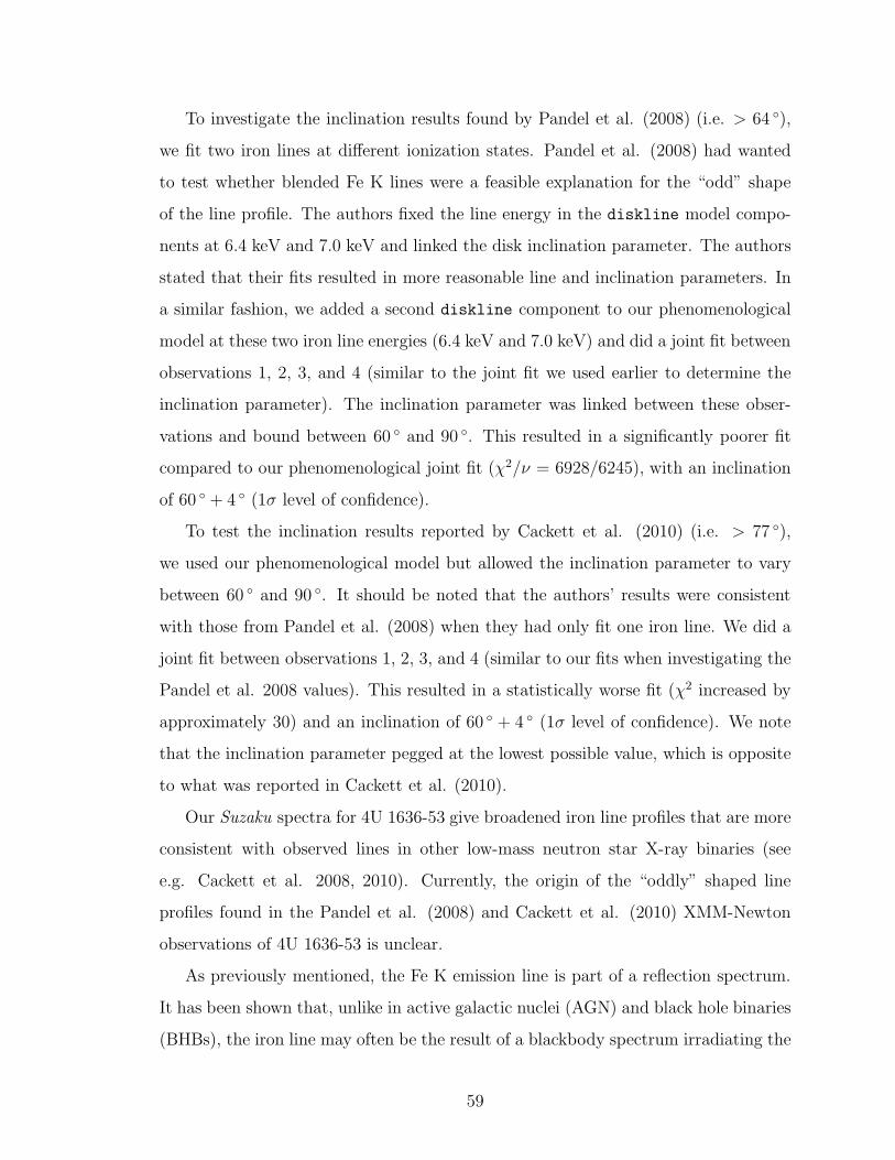
To investigate the inclination results found by Pandel et al. (2008) (i.e. > 64 ),

we fit two iron lines at different ionization states. Pandel et al. (2008) had wanted

to test whether blended Fe K lines were a feasible explanation for the “odd” shape

of the line profile. The authors fixed the line energy in the diskline model compo-

nents at 6.4 keV and 7.0 keV and linked the disk inclination parameter. The authors

stated that their fits resulted in more reasonable line and inclination parameters. In

a similar fashion, we added a second diskline component to our phenomenological

model at these two iron line energies (6.4 keV and 7.0 keV) and did a joint fit between

observations 1, 2, 3, and 4 (similar to the joint fit we used earlier to determine the

inclination parameter). The inclination parameter was linked between these obser-

vations and bound between 60 and 90 . This resulted in a significantly poorer fit

compared to our phenomenological joint fit (χ2/ν = 6928/6245), with an inclination

of 60 + 4 (1σ level of confidence).

To test the inclination results reported by Cackett et al. (2010) (i.e. > 77 ),

we used our phenomenological model but allowed the inclination parameter to vary

between 60 and 90 . It should be noted that the authors’ results were consistent

with those from Pandel et al. (2008) when they had only fit one iron line. We did a

joint fit between observations 1, 2, 3, and 4 (similar to our fits when investigating the

Pandel et al. 2008 values). This resulted in a statistically worse fit (χ2 increased by

approximately 30) and an inclination of 60 + 4 (1σ level of confidence). We note

that the inclination parameter pegged at the lowest possible value, which is opposite

to what was reported in Cackett et al. (2010).

Our Suzaku spectra for 4U 1636-53 give broadened iron line profiles that are more

consistent with observed lines in other low-mass neutron star X-ray binaries (see

e.g. Cackett et al. 2008, 2010). Currently, the origin of the “oddly” shaped line

profiles found in the Pandel et al. (2008) and Cackett et al. (2010) XMM-Newton

observations of 4U 1636-53 is unclear.

As previously mentioned, the Fe K emission line is part of a reflection spectrum.

It has been shown that, unlike in active galactic nuclei (AGN) and black hole binaries

(BHBs), the iron line may often be the result of a blackbody spectrum irradiating the

59

accretion disk in neutron star LMXBs (Ballantyne 2004, D’Ai et al. 2010, Cackett

et al. 2010). This blackbody spectrum is most likely caused by thermal emission

from the neutron star’s surface or boundary layer. Thus, this assumes that the

blackbody component can dominate the flux that ionizes iron (in the energy band

7.0 keV− 20 keV). Such assumptions have been supported by previous spectral fits

(see e.g. Ballantyne & Strohmayer 2004, Cackett et al. 2010). In Figure 3.6 we

have plotted the iron line flux as a function of broadband flux (0.5−30 keV), ionizing

broadband and blackbody flux (7−20 keV), and spectral hardness (5−12 keV)/(3−5

keV) to demonstrate its response (or lack thereof) across our all five observations (and

spectral states). As can be seen in the top panels, there seems to be a fairly weak

response in the strength of the iron line flux to spectral hardness and total broadband

flux; this may be due to our observations being in a narrow range of spectral states.

Note that the iron line flux for observation 5 is treated as an upper limit.

To get a relation between the different fluxes, we determined the best-fit first order

polynomials to the data points for observations 1−4 using the Levenberg-Marquardt

least-squares minimization (note that observation 5 was not included in the calcula-

tions). For the ionizing broadband and blackbody fluxes, the slopes are approximately

7.1 x 10−4 and 5.5 x 10−4, respectively. We also test to see if there is a correspon-

dence between the iron line flux and the ionizing fluxes. We used the Interactive

Data Language (IDL) function r correlate to calculate the Spearman’s rank cor-

relation coefficient, ρ (ranging between -1 and 1). This resulted in ρ = 0.9 for both

the ionizing broadband and blackbody fluxes, respectively, which indicates a positive

correlation with the iron line flux as per expectations. But, this correlation is not

very significant in these data because a coefficient of zero can only be ruled out at

the 1.6σ level of confidence (as determined by the ρ value) for both ionizing fluxes.

The primary results of this chapter use diskline as the main relativistic line

model. Concern may lie in the fact that this model does not take light-bending

effects into account (Fabian et al. 1989). In order to check our diskline results, we

employed similar fits using the self-consistent kyrline model (Dovciak et al. 2004).

This model simulates relativistic line emission from an accretion disk and includes

60

spin as a free parameter. When bound by the same parameter values (e.g. 36 ≤

inclination ≤ 60 , spin frozen at zero, lower limit of inner disk radius set at 6 RG),

the kyrline joint fit was statistically comparable to the diskline fit and had similar

parameter values (χ2/ν = 6648/6237 ∼ 1.07). Also, when the inclination was allowed

to be a completely free parameter, it resulted in a lower inclination value (27+5−4

;

similar to the lower inclination found using diskline).

We also fit the kyrline model to our Suzaku data allowing the inner disk radius to

extend fully to 1 RG, the spin parameter to vary between 0 and 0.3, and the inclination

to be a free parameter. This resulted in a 0 inclination with a higher spin value (0.3)

and an inner disk radius at the lower limit (1 RG) (χ2/ν = 6608/6236 ∼ 1.06). The

value of the inner disk radius suggests a 2.1 km radius for a 1.4M⊙ neutron star and

a 3.0 km radius for a 2.0M⊙ neutron star. Note that these results are in agreement

with those from additional fits using the kerrdisk line model in which a higher spin

value (0.3) is still preferred with the disk extending to the innermost stable circular

orbit (Brenneman & Reynolds). The smaller inner disk radii implied by higher spin

parameters are the product of our data’s modest sensitivity, particularly above 8 keV.

These results are supported by those from Cackett et al. 2010 wherein the data had

higher sensitivity and the inner disk radii were found to confidently exclude 6 RG in

some cases.

While our primary results are model dependent, they are indeed consistent. Ad-

ditionally, when bound by the same parameter values, our results are in agreement

with those from the kyrline model. We note that our inner disk radius values (and

upper limits) using diskline do not allow for tight constraints on the neutron star

radius (see Table 3.4). However, observation 2, which has the tightest inner disk

radius constraint (Rin = 6.0+0.2 RG), gives a radius of 12 km for a 1.4M⊙ neutron

star.

Since the Fe K emission line arises as part of a disk reflection spectrum, we also

fit a neutron star disk reflection model (see Ballantyne & Strohmayer 2004) to the

Suzaku spectra of 4U 1636-53 as a self-consistency measure. Reflection models have

been used previously in a number of neutron star LMXBs (e.g. D’Ai et al. 2010,

61

Cackett et al. 2010). The reflection model we used assumes solar abundances and a

constant-density slab (nH = 1015 cm−3) that is illuminated by a blackbody (bbrefl;

Ballantyne 2004). Since the blackbody component is included within the reflection

model, this component was removed from the continuum model. Also, please note

that the emission lines are already included within the reflection model and we do not

need to include a line component separately in the spectral model. Other spectral

parameters within this model include the log of the ionization parameter, ξ, the

reflection fraction (Ω/2π) and the reflection normalization (see Cackett et al. 2010

for details). All were left completely free. Note that ξ = 4πFX/nH where nH is

the hydrogen number density in the disk, and FX is the flux (Ballantyne 2004).

We relativistically blurred the reflection model by convolving it with the rdblur

model in XSPEC. The rdblur model component generates relativistic effects for the

reflection model. This results in a “smooth” model spectrum that has taken into

account relativistic effects present at the inner accretion disk (see XSPEC 12.6.0

User’s Guide).

We fit observations 1, 2, 3, and 4 individually with the reflection model (Table

3.5). The model parameters were not well constrained by the data. Of particular

note was the relatively high reflection fraction (pegging at the upper bound, Ω/2π

> 1.0) found in each observation. Cackett et al. (2010) have used such reflection

models for 4U 1636-53 and achieved reflection fraction values in the range 0.1−0.3

(with the exception of one observation), which suggest that a reasonable fraction of

the ionizing flux is intercepted by the accretion disk and re-emitted. However, such

moderate values (i.e. 0.3) have statistically worse model fits (with an increase in χ2

> 40) than those with high reflection fraction values (> 1.0) using our Suzaku data .

A possible explanation for our unphysical values for the reflection fraction is that

the blackbody component does not completely dominate the ionizing flux (7.0−20

keV). Our chosen model assumes that X-ray reflection arises from illumination of the

accretion disk by a blackbody, leading to Fe K emission. It has been suggested that

this blackbody component may be due to emission from the boundary layer between

the inner accretion disk and the neutron star surface (see e.g. Sunyaev & Shakura

62

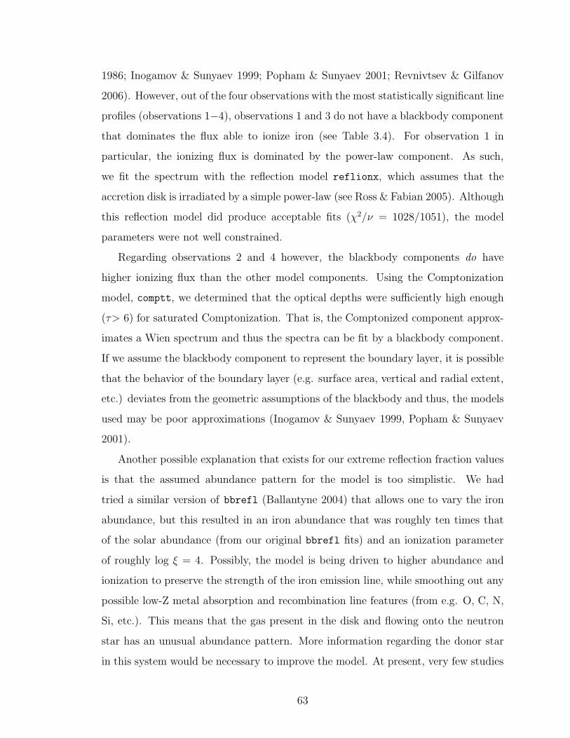
1986; Inogamov & Sunyaev 1999; Popham & Sunyaev 2001; Revnivtsev & Gilfanov

2006). However, out of the four observations with the most statistically significant line

profiles (observations 1−4), observations 1 and 3 do not have a blackbody component

that dominates the flux able to ionize iron (see Table 3.4). For observation 1 in

particular, the ionizing flux is dominated by the power-law component. As such,

we fit the spectrum with the reflection model reflionx, which assumes that the

accretion disk is irradiated by a simple power-law (see Ross & Fabian 2005). Although

this reflection model did produce acceptable fits (χ2/ν = 1028/1051), the model

parameters were not well constrained.

Regarding observations 2 and 4 however, the blackbody components do have

higher ionizing flux than the other model components. Using the Comptonization

model, comptt, we determined that the optical depths were sufficiently high enough

(τ> 6) for saturated Comptonization. That is, the Comptonized component approx-

imates a Wien spectrum and thus the spectra can be fit by a blackbody component.

If we assume the blackbody component to represent the boundary layer, it is possible

that the behavior of the boundary layer (e.g. surface area, vertical and radial extent,

etc.) deviates from the geometric assumptions of the blackbody and thus, the models

used may be poor approximations (Inogamov & Sunyaev 1999, Popham & Sunyaev

2001).

Another possible explanation that exists for our extreme reflection fraction values

is that the assumed abundance pattern for the model is too simplistic. We had

tried a similar version of bbrefl (Ballantyne 2004) that allows one to vary the iron

abundance, but this resulted in an iron abundance that was roughly ten times that

of the solar abundance (from our original bbrefl fits) and an ionization parameter

of roughly log ξ = 4. Possibly, the model is being driven to higher abundance and

ionization to preserve the strength of the iron emission line, while smoothing out any

possible low-Z metal absorption and recombination line features (from e.g. O, C, N,

Si, etc.). This means that the gas present in the disk and flowing onto the neutron

star has an unusual abundance pattern. More information regarding the donor star

in this system would be necessary to improve the model. At present, very few studies

63

have been done on the binary companion (see e.g. Casares et al. 2006).

A final possibility is that our implausibly high reflection fractions partially result

from the cross-calibration of the XIS and HXD (as mentioned earlier). Our fits

indicate that flux levels between the two may differ by ≤ 20%. While we have

properly accounted for these flux differences by including a normalization constant

in our fits, possible flux uncertainties may inhibit strong constraints given that the

high energy reflection flux is low in most neutron star systems.

3.3.3 kHz QPO Results

Each of the accompanying RXTE observations showed one or two significant kHz

QPOs in their power spectra. The frequencies of the kHz QPOs can be found in

Table 3.2. The lower and upper kHz QPOs can only be unambiguously identified

in observation 3, the only one in which both are present. However, based on a

comparison with published power spectra (Altamirano et al. 2008; see Belloni et al.

2005 for details on single kHz QPO detections), we identify the peak in observation

1 as upper kHz QPOs and the ones in observations 4 and 5 as lower kHz QPOs.

The frequencies given in parentheses do not represent actual detections, but are

calculated from the detected QPOs assuming an average peak separation of 300 Hz

(Jonker et al. 2002; Mendez & Belloni 2007). Please note that this average peak

separation should be simply viewed as a typical value. Comparing the location of the

observations in the CD/HID with the frequencies in Table 3.2 we find a monotonic

increase in QPO frequencies along the CD/HID track (from hard to soft) consistent

with previous results (see e.g. van der Klis 2006 and references therein). If we include

the reconstructed frequencies, we obtain an increase in the lower and upper kHz QPOs

by factors of ∼2.8 and ∼1.9, respectively.

3.4 Discussion

We have analyzed five Suzaku observations of the neutron star X-ray binary 4U 1636-

53, which captured the source when it was in the island (transitional) and medium-

luminosity banana (soft) states (see Figure 3.1). In 4 of these 5 observations, a

64

broad Fe K emission line is detected (employing a 3σ cut-off threshold). For the

four cases in which the emission line profiles are clearest (observations 1−4), we use

the model diskline in XSPEC. The diskline model is an imperfect but sufficient

representation of lines expected around a neutron star, and permits constraints on

the inner disk radius, which in turn give an upper limit on the neutron star radius.

Our most stringent constraint corresponds to a radius of 12 km for a 1.4 M⊙ neutron

star.

Although we did not observe a monotonic evolution in time from the island state

to banana state (RXTE monitoring suggests that the source went through two full

state transition cycles during our Suzaku campaign), our results do not provide strong

positive evidence for a change in the inner disk radius. A stronger statement is

prevented by results obtained from fits to Observation 1, wherein a large inner disk

radius cannot be excluded. Moreover, since 4U 1636-53 was only observed between the

island state and medium-luminosity banana state, more observations in other spectral

states (e.g. the extreme island, or hard, state) may be necessary to completely resolve

this question.

In the sections that follow, the strengths and limitations of our analysis, and

possible implications, are briefly explored.

3.4.1 The Inner Disk Radius and State Transitions

Our results are consistent with a picture wherein the inner radius of the accretion disk

does not change appreciably across different spectral states. D’Ai et al. (2009) and

Cackett et al. (2010) have reached similar conclusions for a number of neutron star

low-mass X-ray binaries, including GX 340+0 and 4U 1636-53. Cackett et al. (2010)

concluded that there was no clear correlation between the extent of the inner disk

radius and source luminosity. However, broadband spectra were not used to study 4U

1636-53 in that analysis. The broader spectral coverage of our Suzaku observations

did yield strong evidence in favor of disk truncation. Moreover, the inner disk radius

constraints derived from our fits to the disk continuum match those from obtained

by modeling the iron line. Evidence for stable inner disk radii across spectral states

65

is mounting in black hole systems (see Miller et al. 2006b, Reis, Miller, & Fabian

2010, Steiner et al. 2010), and it is interesting that the accretion flow in neutron star

LMXBs may behave similarly.

A constant inner disk radius across spectral states (i.e. extreme island, island, ba-

nana) would have significant implications for our understanding of state transitions

in neutron star LMXBs. Currently, the origins of the flux variability observed in

these systems remains uncertain, although multiple hypotheses have been proposed.

At first glance, the most likely culprit seems to be the accretion disk, which is related

to accretion flow parameters such as mass accretion rate M , etc. Possibly, changes in

the mass accretion rate could affect the extent of the inner disk radius and thereby

cause state transitions. The apparent constancy of the inner disk radius, as measured

from the iron line profile and the disk continuum, is of particular interest when one

considers the (apparently substantial) changes in the kHz QPO frequencies (see Table

3.2). Many interpretations of kHz QPOs require that one of the frequencies corre-

sponds to the Keplerian frequency at the inner disk radius (see Miller et al. 1998).

In such a framework, the kHz QPOs in our RXTE observations paint a very different

picture of the inner disk behavior than our spectral results. The consistency of inner

disk radius results from both the Fe K line, disk continuum, and kHz QPO measure-

ments is still a source of debate (see e.g. Cackett et al. 2008, 2010 and references

therein). One possibility that is consistent with the data is that the frequency of the

kHz QPOs trace the mass accretion rate more closely than the inner disk radius.

Previous studies of neutron star LMXBs have investigated how spectral states

are affected by changes in the inner disk radius and/or M . For example, Lin et al.

(2010) observed the atoll source 4U 1705-44 and determined that the data diverged

from the L α T 4 relation for the soft state, which is similar to what we found in

our data from 4U 1636-53, albeit in the transitional state (observation 1). Since

this relation signifies a constant inner disk radius, the authors concluded that the

deviations might be due to disk truncation or a spectral hardening factor (see e.g.

Davis et al. 2006). A higher value for the color correction factor might be appropriate

in hard spectral states (Merloni, Fabian, & Ross 2000), and that would make the disk

66

properties measured in Observation 1 more consistent with a constant emitting area.

Moreover, Barret & Olive (2002) concluded that there was no correlation between

the instantaneous M and the inner disk radius for this source.

Lin et al. (2009) and Homan et al. (2010) observed the neutron star LMXB XTE

J1701-462, which is a unique source because it demonstrates both Z and atoll source

characteristics. A goal of the analyses was to determine the physical parameter(s)

causing the transition between these two source types such as M (Homan et al.

2007), neutron star magnetic field strength (Hasinger & van der Klis 1989), and

viewing angle (Kuulkers & van der Klis 1995). The authors concluded that indeed

the Z/atoll transition in XTE J1701-462 was due to changes in M ; there was no

significant variation in M as the source progressed along the Z track with the the

opposite being true for the atoll track. This conclusion is consistent with results from

Rykoff et al. (2010), which suggest that M may not increase monotonically with

spectral state in Z sources as has been assumed (see e.g. Hasinger 1990). Moreover,

Strohmayer & Bildsten (2006) have shown from X-ray burst observations that there

is no clear trend between M and spectral state in neutron stars.

Compared to the studies above, if we make the naive assumption that the total

inferred luminosity (see Sec. 3.3) is a simple function of M , then there may be a rough

correlation between M and spectral state for the atoll source 4U 1636-53. However,

our data provide only incomplete evidence since we have only observed this source in

a narrow range of spectral states.

The detection of iron emission lines and high frequency QPOs in 4U 1636-53

strongly supports a disk origin for both features. Previous studies have suggested

that broad iron lines could be the result of scattering in an outflow i.e. a disk wind

as opposed to disk reflection (see e.g. Laming & Titarchuk 2004, Shaposhnikov et

al. 2009). Titarchuk et al. (2009) stated that outflowing gas should suppress high-

frequency modulations in the disk wind model. However, this is not the case in 4U

1636-53, where the high frequency QPOs with high Q-values are observed. Thus, the

fact that we detect both Fe K emission lines and high frequency QPOs rules out the

possibility of iron line formation in a disk wind.

67

3.4.2 Alternative Possibilities for State Transitions

It is possible that other physical parameters/mechanisms may be the cause of spectral

state transitions, such as the corona, a boundary layer, a magnetosphere, or a jet

(van der Klis 2006, Fender 2006, Lin et al. 2010). Changes in the corona (e.g. in

density, ionization, etc.) might be reflected by changes in the inner disk radius (see

e.g. Esin et al. 1997 for black hole binaries). However, the constant radius that we

observe might suggest that the corona is not closely linked with the kinematics in the

accretion disk. Neutron star surface (or boundary layer) emission distortions may

also be the cause of kHz QPOs since physical processes such as radial and non-radial

neutron star surface oscillations, nuclear-burning processes causing temporary surface

characteristics, and magnetohydrodynamic effects have all been suggested as origins

of the observed variability (see van der Klis 2006 and references therein).

Our Suzaku data cannot rule out these boundary layer possibilities because they

require assumptions about the neutron star equation of state (EOS); our upper limits

on the neutron star radius in 4U 1636-53 cannot provide significant constraints on

any EOS models. For neutron stars with sufficiently strong magnetic fields (e.g. 1012

G), the accretion disk may be truncated at the magnetospheric radius and possibly

cause aperiodic variability (see van der Klis 2006 and references therein). For that

situation, however, a constant inner disk radius would not explain the range between

which kHz QPO frequencies vary, as kHz QPO values increase with spectral state

(i.e. progressing from the extreme island state to banana state; see van der Klis 2006:

Fig. 2.9). Also, this situation would not be the case for neutron star LMXBs like 4U

1636-53 since they most likely have low magnetic fields (107−109 G). The role of jets

in producing the observed variability in neutron star LMXBs remains uncertain due

to a majority of the sources (particularly atolls) not being detected in the radio band

(see e.g. Migliari & Fender 2006).

3.4.3 Neutron Star Equation of State

Our analysis of iron line profiles in a source that exhibits kHz QPOs allows us to

estimate the mass of the neutron star in 4U 1636-53 (Piraino et al. 2000, Cackett et

68

al. 2008). This is an important step towards getting constraints on the nature of ultra-

dense matter. Figure 3.1 shows the RXTE observations overlapping with, or closest

to, our Suzaku observations. Specifically, in observation 3 both lower and upper kHz

QPO frequencies were detected (see Table 3.2). Assuming that the upper kHz QPO

frequency represents the orbital frequency at the inner edge of the accretion disk

(although this may not always be the case, see Sec. 3.4.1), we can use the expression,

νorb = (1/2π)√

GM/r3, to get a constraint on the mass. Using our value of the inner

disk radius, r (6RG), from our observations results in M≤ 2.4M⊙. Furthermore, if

we use the highest frequency QPO observed in 4U 1636-53 (1220 Hz; see van der

Klis et al. 1996; Miller et al. 1998: Table 1), we get M≤ 1.8M⊙. Although our

range of estimates for the neutron star mass in 4U 1636-53 is broad, the results are

encouraging. Future simultaneous spectral and timing observations for this source

can help obtain better mass constraints.

3.4.4 Conclusions

The results of our detailed analysis of five Suzaku observations of the neutron star

LMXB 4U 1636-53 can be summarized as follows:

• In four observations, a broad Fe K emission line is detected (implementing a 3σ

detection threshold). The breadth of the line profile indicates that gravitational

and relativistic Doppler broadening are present.

• The detection of Fe K emission lines and kHz QPOs in simultaneous data signals

that the line cannot arise through scattering in a dense outflow that would

otherwise scatter-away the variability.

• The inner disk radius, constrained independently using the broad Fe K line and

thermal disk continuum, is consistent with a constant value in the island and

medium-luminosity states. However, more observations of the source in other

spectral states, such as the extreme island state and high luminosity banana

state, may be necessary to resolve this matter. Deeper observations may also

determine the physical processes that act to drive variability.

69

• We estimate a neutron star mass of M≤ 2.4M⊙ based on the iron line profile

and upper kHz QPO frequencies.

• Fitting a neutron star disk reflection model to the data did not permit strong

parameter constraints. We obtained unreasonably high values for the reflection

fraction. This could be due to a number of causes, including (1) the blackbody

component not completely dominating the ionizing flux, (2) the boundary layer

deviating from the geometric assumptions of the blackbody, (3) inadequate data

on the donor star, and/or (4) flux uncertainties of the XIS and HXD.

70

Observation # ObsID Date Time (UT) XIS, PIN (ks) BurstsObservation 1 401050010 09-02-2007 09:18:22 12.0, 21.0 2Observation 2 401050020 22-02-2007 07:05:38 19.9, 35.2 1Observation 3 401050030 01-03-2007 01:01:07 19.3, 47.1 5Observation 4 401050040 27-03-2007 11:31:36 16.0, 27.6 2Observation 5 401050050 29-03-2007 11:19:47 6.1, 11.4 2

Table 3.1. Suzaku observations of 4U 1636-53. This table is a summary of the Suzaku observationsfor 4U 1636-53. Column 4 shows the net exposures from XIS and HXD-PIN detectors. Column 6shows the number of bursts. The amount of time excluded before/after each burst peak was up to100 sec and 320 sec, respectively.

lower kHz QPO upper kHz QPOSuzaku obs. MJD RXTE obs. MJD Overlap νmax (Hz) Q r.m.s. (%) νmax (Hz) Q r.m.s. (%)

Observation 1 54140.388 92023-01-74-10 54140.009 No (294) — — 594+18−12 9+6

−3 9.8±1.8Observation 2 54153.296 92023-01-81-10 54154.030 Yes 930±2 77+44

−24 4.3±0.7 (1230) — —Observation 3 54160.042 92023-02-17-00 54160.052 Yes 611±14 12+14

−6 5.8±1.4 941±13 12+6−4 8.1±1.2

Observation 4 54186.480 92023-01-05-20 54186.762 Yes 721.5±1.0 44.4±5.4 9.1±0.4 (1021.5) — —Observation 5 54188.472 92023-01-06-20 54188.795 No 853.6±1.1 56±13 7.9±0.6 (1153.6) — —

Table 3.2. Suzaku and RXTE observations of 4U 1636-53. This table has the RXTE observationsthat showed lower and/or upper frequency QPOs and coincided the most with our Suzaku observa-tions are presented above. As shown, three Suzaku and RXTE observations overlap. The frequenciesgiven in parentheses are not actual detections, but are calculated from the detected QPOs assumingan average peak separation of 300 Hz (Jonker et al. 2004; Mendez & Belloni 2007). We measured95% upper limits on the r.m.s. amplitude of 4.8% (Q fixed at 10) and 4.1% (Q fixed at 50), in the200–1500 Hz frequency range.

Parameter Obs. 1 Obs. 2 Obs. 3 Obs. 4 Obs. 5Line energy (keV) 6.3(3) 5.5(1) 5.5(1) 5.7(2) 5.4(6)

Sigma (keV) 1.2−0.04 1.2−0.1 1.2−0.03 1.2−0.1 1.2−0.2

Normalization (10−3) 3.1(5) 6.3(9) 5.4(8) 4.7(9) 4(2)χ2/ ν 1070/1051 (1.02) 2137/1934 (1.10) 1817/1674 (1.09) 1567/1587 (0.99) 979/1040 (0.94)

Table 3.3. Gaussian parameters. This table shows the Gaussian models were fit to the data fromobservations 1−5. The line energy and σ were allowed to vary between 4−7.5 keV and 0−1.2 keV,respectively. The normalization parameter was left completely free. Although the Gaussian modeldoes fit the data well in several cases, the line energy is always less than 6.4 keV, indicating thatrelativistic broadening and gravitational redshift are present and that a relativistic line model isneeded. All errors are 90% confidence errors.

71

Parameter Obs. 1 Obs. 2 Obs. 3 Obs. 4 Obs. 5NH (1022cm−2) (0.36) (0.36) (0.36) (0.36) (0.36)Power-law index 1.95(2) 2.44(2) 2.20(1) 2.41(2) 2.49(5)

Power-law norm (10−2) 27.3(6) 24.0(5) 30.5(5) 20.7(5) 18(1)FluxPL (10−10) (7−20 keV) 5.3(1) 1.37(3) 3.18(5) 1.27(3) 0.95(5)

FluxPL (10−10) (0.5−30 keV) 19.3(4) 9.7(2) 15.8(3) 8.7(2) 7.3(4)Disk blackbody (keV) 0.24(2) 0.976(8) 0.80(1) 0.90(1) 0.91(2)

Disk blackbodycor (keV) 0.14(1) 0.574(5) 0.47(1) 0.53(1) 0.54(2)Disk blackbody norm 3(1) (x 103) 115(1) 129(3) 101(2) 111(9)

Rin from disk blackbody (km) 4(1) (x 101) 7.2(1) 7.6(2) 6.7(1) 7.0(6)Rin,cor from disk blackbody (km) 6(1) (x 101) 10.4(1) 11.0(3) 9.7(1) 10.0(9)

Rin (GM/c2) for 1.4 M⊙ 19(5) 3.5(1) 3.7(1) 3.2(1) 3.4(3)Rin,cor (GM/c2) for 1.4 M⊙ 28(5) 5.0(1) 5.3(1) 4.7(1) 4.8(4)Rin (GM/c2) for 2.0 M⊙ 14(4) 2.4(1) 2.6(1) 2.3(1) 2.4(2)

Rin,cor (GM/c2) for 2.0 M⊙ 20(3) 3.5(1) 3.7(1) 3.3(1) 3.4(3)FluxDisk (10−11) (7−20 keV) 0.01(1) 3.10(3) 0.39(1) 1.26(2) 1.5(1)FluxDisk (10−9) (0.5−30 keV) 0.10(3) 1.98(1) 0.911(9) 1.27(1) 1.4(1)

Blackbody (keV) 1.8(3) 2.08(2) 1.99(4) 2.06(3) 2.05(6)Blackbody norm (10−2) 0.08(2) 1.70(1) 0.80(1) 1.14(2) 1.35(4)

FluxBB (10−10) (7−20 keV) 0.32(7) 7.50(4) 3.31(4) 4.90(2) 5.8(2)FluxBB (10−9) (0.5−30 keV) 0.07(1) 1.42(1) 0.66(1) 0.95(2) 1.13(3)

Line energy (keV) 6.6(2) 6.40+.02 6.40+.06 6.4+0.1 (6.40)Equivalent width (eV) ( x 101) 10(4) 6(2) 6(2) 8(2) < 8

Rin (GM/c2) 6.0+30 6.0+0.2 6+4 6+7 (6)Rin (km) from Fe K line for 1.4 M⊙ 12+52 12.0+0.4 12+8 12+14 ...Rin (km) from Fe K line for 2.0 M⊙ 18+90 18.0+0.6 18+12 18+21 ...

Rout (1000) (1000) (1000) (1000) (1000)Emissivity index, β (-3) (-3) (-3) (-3) (-3)Inclination (deg) (36) 36+2 36+5 36+4 (36)

Normalization (10−4) 7(3) 12(3) 7(2) 9(3) < 13Total Flux (10−10) (7−20 keV) 5.6(1) 9.18(5) 6.5(6) 6.3(4) 6.9(8)Total Flux (10−9) (0.5−30 keV) 2.11(5) 4.4(2) 3.2(3) 3.1(2) 3.3(4)

χ2/ ν 959/1050 (0.91) 2226/1933 (1.15) 1884/1673 (1.13) 1606/1586 (1.01) 984/1042 (1.00)

Table 3.4. Phenomenological parameters. This table shows the phenomenological model (i.e. tbabsx (powerlaw +diskbb +bbody+ diskline)) fits to the broadband spectra (XIS and PIN) of the5 Suzaku observations. The horizontal lines separate the model components. Parameter values inparentheses were fixed. A constant was allowed to float between the XIS and PIN data. All fluxesquoted above are “unabsorbed” fluxes and are given in units of erg cm−2s−1. Fluxes from the modelcontinuum components are also listed. For observation 5 a fiducial iron line, with the inner radiusand inclination parameters fixed to “common” values based on the joint fits for observations 1,2,3and 4, was fit to the data; thus, the diskline component results are upper limits. Note that forobservation 1, the inclination parameter was fixed in order to improve parameter constraints. Whencalculating the inner disk radius from diskbb, an inclination of 36 was assumed. For a bettercomparison with the inner disk radii from the Fe K line, Rin (in units of GM/c2) is calculated fora neutron star of 1.4 M⊙ and 2.0 M⊙ for the blackbody component. Also, for the Fe K line, Rin

(in units of km) was calculated assuming a mass of 1.4 M⊙ and 2.0 M⊙. Note that in additionto the raw values listed for the disk blackbody component, we have also reported color correctedvalues (labeled with subscript “cor”). That is, we applied a color correction factor (f = 1.7) to thetemperature (α 1.0/f) and inner disk radii (α f2/2.0) for the blackbody component (see Section3.3.2). Errors given in parentheses are symmetric (90 % confidence) errors in the last significantdigit.

72

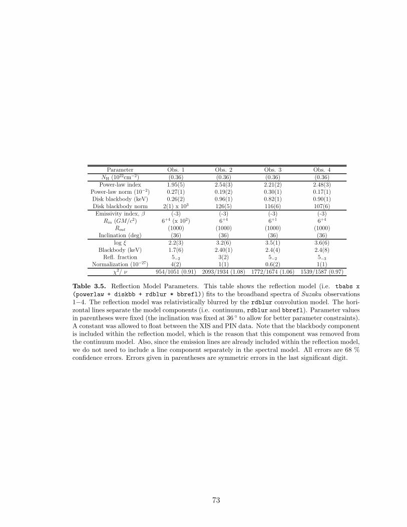
Parameter Obs. 1 Obs. 2 Obs. 3 Obs. 4NH (1022cm−2) (0.36) (0.36) (0.36) (0.36)Power-law index 1.95(5) 2.54(3) 2.21(2) 2.48(3)

Power-law norm (10−2) 0.27(1) 0.19(2) 0.30(1) 0.17(1)Disk blackbody (keV) 0.26(2) 0.96(1) 0.82(1) 0.90(1)Disk blackbody norm 2(1) x 103 126(5) 116(6) 107(6)Emissivity index, β (-3) (-3) (-3) (-3)

Rin (GM/c2) 6+4 (x 102) 6+4 6+1 6+4

Rout (1000) (1000) (1000) (1000)Inclination (deg) (36) (36) (36) (36)

log ξ 2.2(3) 3.2(6) 3.5(1) 3.6(6)Blackbody (keV) 1.7(6) 2.40(1) 2.4(4) 2.4(8)

Refl. fraction 5−2 3(2) 5−2 5−3

Normalization (10−27) 4(2) 1(1) 0.6(2) 1(1)χ2/ ν 954/1051 (0.91) 2093/1934 (1.08) 1772/1674 (1.06) 1539/1587 (0.97)

Table 3.5. Reflection Model Parameters. This table shows the reflection model (i.e. tbabs x

(powerlaw + diskbb + rdblur * bbrefl)) fits to the broadband spectra of Suzaku observations1−4. The reflection model was relativistically blurred by the rdblur convolution model. The hori-zontal lines separate the model components (i.e. continuum, rdblur and bbrefl). Parameter valuesin parentheses were fixed (the inclination was fixed at 36 to allow for better parameter constraints).A constant was allowed to float between the XIS and PIN data. Note that the blackbody componentis included within the reflection model, which is the reason that this component was removed fromthe continuum model. Also, since the emission lines are already included within the reflection model,we do not need to include a line component separately in the spectral model. All errors are 68 %confidence errors. Errors given in parentheses are symmetric errors in the last significant digit.

73

1.6 2

0.8

1.2

Soft color

Har

d co

lor

b

transitional(island)

soft (banana)

200 400 600 800

Count rate (cts/s)

cObs. 1Obs. 2Obs. 3Obs. 4Obs. 5

100 150 200

0.8

1.2

MJD − 54000 (Days)

Har

d co

lor

a

Figure 3.1. Long-term hardness, CD, and hardness-intensity curves. This plot shows a long-termhardness curve (a), a color-color diagram (soft color: [4.0–7.3 keV]/[2.4–4.0 keV], hard color: [9.8–18.1 keV]/[7.3–9.8 keV]) (b), and a hardness-intensity curve (average count rate: (2.4–30.0 keV))(c) of 4U 1636-53 that is created from RXTE data. The count rate is the RXTE/PCU2 count rate.Colors and count rates were corrected for changes in detector gain and response using observationsof the Crab. An early observation of the Crab (Obs. ID. 10200-01-01-00, MJD 50802) was used asour reference point. The red points represent the approximate locations of the Suzaku observations.Note that the Suzaku observations were spread over two transition cycles.

74

2 4 6 8 100.9

11.

1

ratio

Energy (keV)

2 4 6 8 100.9

11.

1

ratio

Energy (keV)

2 4 6 8 100.9

11.

1

ratio

Energy (keV)

2 4 6 8 100.9

11.

1

ratio

Energy (keV)

2 4 6 8 100.9

11.

1

ratio

Energy (keV)

Figure 3.2. Iron line profiles. This plot shows, in order from top to bottom: iron line profiles withrespect to the continuum from Suzaku 4U 1636-53 observations 1−5, respectively. These data/modelratios were formed by ignoring the Fe K region, fitting the continuum, and then including the ironband. Note that for this figure, apparent lack of data points above 7 keV in observations 1 and 5can be attributed to grouping the data to a minimum of 300 counts per bin.

75

1 102 5 200.9

11.

1

ratio

Energy (keV)

1 102 5 200.9

11.

1

ratio

Energy (keV)

1 102 5 200.9

11.

1

ratio

Energy (keV)

1 102 5 200.9

11.

1

ratio

Energy (keV)

1 102 5 200.9

11.

1

ratio

Energy (keV)

Figure 3.3. Data/model ratios of the Suzaku spectra of 4U 1636-53. This plot shows the Suzakuspectra of 4U 1636-53 from all 5 observations fitted with the diskline model. The curves withinthe 0.7−10 keV energy range represent the data from the XIS detectors. The curves within the12−30 keV energy range represent the data from the PIN detector. The data/model ratios (in orderfrom top to bottom) are from observations 1, 2, 3, 4 and 5, respectively. The accompanying spectralfits can be found in Figure 3.4.

76

1 102 5 2010−

510

−4

10−

30.

010.

1

Pho

tons

cm

−2

s−1

keV

−1

Energy (keV)

1 102 5 2010−

510

−4

10−

30.

010.

1

Pho

tons

cm

−2

s−1

keV

−1

Energy (keV)

1 102 5 2010−

510

−4

10−

30.

010.

1

Pho

tons

cm

−2

s−1

keV

−1

Energy (keV)

1 102 5 2010−

510

−4

10−

30.

010.

1

Pho

tons

cm

−2

s−1

keV

−1

Energy (keV)

1 102 5 2010−

510

−4

10−

30.

010.

1

Pho

tons

cm

−2

s−1

keV

−1

Energy (keV)

Figure 3.4. The diskline model and components. The bold line represents the overall model andthe dotted lines represent the separate model components for observations 1−5, respectively (top tobottom). For example, from top to bottom at 6 keV for observation 2, the blackbody, the multicolordisk blackbody, the power-law and the diskline model components are shown.

77

Figure 3.5. Blackbody and disk blackbody plots. In this plot, for all Suzaku observations, theblackbody temperature is plotted versus broadband blackbody flux (top panel) and the disk black-body temperature is plotted versus broadband disk blackbody flux (bottom panel). Note that thedisk blackbody values are not color corrected. The crosses represent the data points. The lines showthe L α T 4 relation with constant emitting surface area for various radii. Specifically, the dashed,dotted, and dash-dotted lines represent a radius R = 3.0 km, 1.5 km and 0.4 km for the blackbodycomponent and 30 km, 8.0 km, and 2.0 km for the disk blackbody component, respectively. Therelation is calculated for L=4πR2σT 4. A distance of 6 kpc was assumed. In both plots, the leftmostdata point is observation 1, which deviates significantly from the calculated relation.

78

Figure 3.6. Iron line flux plots. In this plot, for all 5 Suzaku observations, broadband flux (0.5−30keV), spectral hardness (5−12keV)/(3−5 keV), ionizing flux (7.0−20 keV), and blackbody flux areplotted versus Fe line flux. The dotted lines represent the best-fit first-order polynomials to the datapoints. These were determined using the Levenberg-Marquardt least-sqaures minimization. Notethat the Fe line flux for observation 5 is given as an upper limit; this observation was not includedwhen determining the best-fit.

79

CHAPTER 4

Suzaku Observations of the Black Hole H1743-322

in Outburst

4.1 Introduction

H1743-322 was discovered during its 1977-1978 outburst with the High Energy As-

tronomical Observatory-1 (HEAO-1) and Ariel 5 (Doxsey et al. 1977, Kaluzienski &

Holt 1977). Based on its spectral characteristics, H1743-322 was classified as a Galac-

tic X-ray transient by White & Marshall (1984). The 2003 outburst of H1743-322

allowed for two discoveries that provided evidence that this source harbors a black

hole primary. First, Homan et al. (2003) reported the detection of quasi-periodic os-

cillations (QPOs) at 160 Hz and 240 Hz, a 2:3 frequency ratio that is typical for black

hole candidates (e.g. GRO J1655-40: Strohmayer 2001a; GRS 1915+105: Strohmayer

2001b; XTE J1550-564: Miller et al. 2001). Second, Rupen et al. (2003) (see also

Corbel et al. 2005) reported a relativistic jet (v/c≃0.8) in H1743-322, which allows

this source to be termed a “microquasar.”

A disk wind can be key to understanding the nature of the accretion flow in disk

systems (e.g. Proga 2003, Ueda et al. 2009, Ohsuga et al. 2009). In this paper, we

refer to observations of H1743-322 in the soft state and steep power-law state made

in 2003 (Miller et al. 2006a). Previously, Chandra observations of H1743-322 during

its 2003 outburst found evidence of an ionized disk wind in the soft state, in the

form of blue-shifted Fe XXV and XXVI absorption lines (Miller et al. 2006a). Figure

4.1 compares the light curves of H1743-322 when it was observed in the soft state

and the hard state. The apparent difference in counts/sec and hardness between the

two states emphasizes the distinction between spectral states for black hole binaries.

80

Iron aborption lines were absent when Chandra observed H1743-322 in the steep

power-law state. Similar results were obtained from Chandra observations of GRO

J1655-40 (Miller et al. 2006d, Miller et al. 2008a) and GRS 1915+105 (Miller et al.

2008a, Neilson & Lee 2009). The physical mechanism needed to produce such a disk

wind is still being investigated, aided by an extensive theoretical framework (see e.g.

Blandford & Payne 1982, Begelman et al. 1983, Proga et al. 2000). In this chapter,

we report the results of an analysis of the Suzaku X-ray spectra resulting from the

H1743-322 October 2008 outburst. Preliminary results from this observation were

reported in Blum et al. 2008 (ATel # 1841).

4.2 Data Reduction

Suzaku observed H1743-322 on 2008 October 7 starting at 16:19:21 (UT). The ob-

servation duration was approximately 72 ks. The X-ray Imaging Spectrometer (XIS)

pointing position was used. The three detectors constituting the X-ray Imaging Spec-

trometer (XIS0, XIS1, XIS3; energy range 0.2−12 keV) were each operated in 3x3

and 5x5 editing modes; using the 1/4 window mode with a 1.0 sec burst option helped

to limit photon pileup. No timing mode was used. The energy resolution (FWHM)

of the XIS cameras is ∼ 120 eV at 6.0 keV and ∼ 50.0 eV at 1.0 keV. Each CCD

camera has a single CCD chip with an array of 1024 x 1024 pixels, and covers an 18′

x 18′ region on the sky. Each pixel is 24µm square, and the size of the CCD is 25mm

x 25mm. The XIS1 sensor uses a back-side illuminated CCD, while the other two

use a front-side illuminated CCD (e.g. Koyama et al. 2007). XIS on-source times

of approximately 32 ks were achieved. This resulted in a dead-time corrected net

exposure of 16 ks for the XIS cameras.

Soft X-ray spectra within the energy ranges 0.7−1.5 keV and 2.2−10.0 keV were

used. The 1.5−2.2 keV energy range was ignored to avoid systematic errors due to

calibration in the Si band. We used the latest calibration database available at the

time of analysis (CALDB 20090925). From the cleaned event files we extracted the

source light curve and spectrum with xselect. A circle centered on the source with

a radius of 129′′ (123 in pixel units) was used for the source extraction region. A

81

circular, off-source region with a radius of 45′′ (43 in pixel units) was used to extract

the background. The 3x3 and 5x5 mode event files for each XIS detector were loaded

together into xselect. A single source and background spectrum was extracted

from these event files for each XIS detector. The XIS redistribution matrix files

(RMFs) and ancillary response files (ARFs) were created using the tools xisrmfgen

and xissimarfgen available in the HEASOFT version 6.6.2 data reduction package.

The 3x3 and 5x5 mode event files were used to specify good time intervals and the

data was grouped to a minimum of 300 counts per bin using the FTOOL grppha.

The Hard X-ray Detector (HXD) covers the energy range 10.0−700 keV and is

a combination of Positive Intrinsic Negative (PIN) silicon diodes and Gadolinium

Silicate (GSO) phoswich counters. A net exposure of 29 ks was achieved using the

HXD (PIN and GSO) cameras, which were operated in their normal mode. The HXD

features an effective area of ∼ 160 cm2 at 20.0 keV, and ∼ 260 cm2 at 100 keV (e.g.

Takahashi et al. 2007). The HXD time resolution is 61 µs. The HXD-PIN/GSO data

were reprocessed from an unscreened event file with up-to-date calibration databases

in accordance with the Suzaku Data Reduction Guide (CALDB 20090511). The

appropriate response matrices for the XIS aimpoint and background files were down-

loaded from the Suzaku web page. In our analysis, the energy range for the HXD

cameras was restricted to 12.0−200 keV.

4.3 Data Analysis and Results

Using the X-ray spectral fitting software package (XSPEC v. 11.3.2, Arnaud 1996),

the Suzaku H1743-322 spectra from the three XIS detectors and the HXD detector

were fit jointly. A normalizing constant (ranging between 1.0 and 1.1) was allowed

to float between spectra to account for different detector flux zero-points. Our initial

spectral model consisted of an absorbed power-law (χ2/ν = 3348/3095). We used

tbabs in our model to account for photoelectric absorption in the interstellar medium

(ISM). Replacing a simple power-law with a broken power-law provided an improved

fit (χ2/ν = 3053/3093) with Ebreak ≃ 36(2) keV, Γ1 ≃ 1.55(1), and Γ2 ≃ 2.2(1).

The fit results in the 0.7−200 keV band with the absorbed broken power-law model

82

are reported in Table 4.1 with a spectral fit being shown in Figure 4.2 and Figure

4.3. For Figure 4.3 we note that the residuals near 10.0 keV in the XIS spectra are

likely due to calibration uncertainties and not photon pile-up (different size extraction

regions had negligible effect on the resulting spectral fit). The spectral parameters

obtained through our fits for H1743-322 are typical of a Galactic black hole candidate

in the hard state (McClintock & Remillard 2006, Fender & Belloni 2004). Note that

the high equivalent neutral hydrogen column density (2.00(1) x 1022 cm−2) along

the line of sight is consistent with a central Galactic distance to H1743-322 and is

in accordance with the value used by Miller et al. (2006a). The unabsorbed flux

inferred in the 0.5-200 keV band is (7.51 ± 0.08) x 10−9 erg cm−2s−1. Currently,

the mass of H1743-322 and the distance to the source are unknown. But, given its

position near the Galactic center (l ≃ 357.255 , b ≃ −1.833 ) and relatively high

column density, it is reasonable to use a Galactic center distance of 8.5 kpc. Using

this value as an estimate of the distance to the source gives a luminosity of LX = (6.37

± 0.07) x 1037 (d/8.5kpc)2 erg s−1 (we calculated the Galactic ridge X-ray emission

contribution to be negligible and accounted for by our background spectrum). This

calculated luminosity indicates that the source would be 0.08 LEDD for a 6 M⊙ black

hole and 0.05 LEDD for a 10 M⊙ black hole.

A broken power-law may be a phenomenological description of Compton upscat-

tering of disk photons by a central, hot, electron-dominated “corona” (see e.g. Ross

et al. 1999). Therefore, we also fit a Comptonization model (compTT; Titarchuk 1994)

to the broadband Suzaku data. This is an analytic model describing Comptonization

of soft photons in a hot plasma. The approximations used in the model work well

for both the optically thin and thick regimes. Fitting the compTT model resulted in

an electron temperature of kT ≃ 38(5) keV for a disk temperature of kT ≃ 0.25(2)

keV (typical disk temperature for the hard state; see e.g. Miller et al. 2006b). The

reduced χ2 for this Comptonization model was ≃ 3066/3092 (see Table 4.2). Note

that the energy break in our best-fit broken power-law model, which can indicate the

electron temperature of the purported corona, is consistent with the electron temper-

ature in the Comptonization model. Such a corona may be the source of hard X-rays

83

irradiating the accretion disk and producing a reflection spectrum. Additionally, any

spectral state dependence of iron absorption features may suggest a corona with a

changing geometry.

To test for the presence of the X-ray Fe XXV and Fe XXVI absorption lines in

the Suzaku spectrum for H1743-322, we added a Gaussian component to the broken

power-law continuum model. Note that this simple model is useful for estimating

line strengths. We froze the line energy at the theoretical values for Fe XXV (6.70

keV) and Fe XXVI (6.97 keV), respectively. The line width was frozen at zero (due

to the likelihood that the lines would be at least as narrow as those observed with

Chandra; see Miller et al. 2006a) while the line flux normalization parameter (in

units of photons cm−2s−1) was allowed to vary. Error analysis was performed on

the line flux (using the error command) to derive the maximum allowable iron line

normalization at 90% confidence. The line wavelengths, fluxes, and equivalent widths

are listed in Table 4.3. The equivalent width upper limits for both iron absorption

lines were < 3.5 eV.

Based on these results, we conclude that these iron absorption lines were not

present in the Suzaku spectrum for H1743-322 when it was observed in the hard state.

The Miller et al. (2006a) Chandra observations spanned several black hole binary

spectral states, particularly the steep power-law state and the soft state. Similar to

our Suzaku results, the Fe XXV and Fe XXVI absorption lines were absent in the

source’s spectrum in the steep power-law state (equivalent width upper limits < 4.3

eV; see Miller et al. 2006a). For softer states (i.e. the soft state), however, each

detection of Fe XXV and Fe XXVI absorption lines was at the 4 σ level of confidence

or higher (with e.g. equivalent widths of 16(1) eV and 25(3) eV, respectively; see

Miller et al. 2006a: Table 3). Moreover, Miller et al. (2006a) estimated that disk

winds in H1743-322 originated at radii between 102rg and 104rg for a 10 M⊙ black

hole and potentially changed geometry across spectral states. The combined results of

Suzaku and Chandra indicate that there is a spectral state dependence on absorption

lines, and therefore disk winds.

Disk reflection features are common amongst Galactic black hole X-ray spectra

84

(Miller 2007). As shown in Figure 4.4, there is a potential Fe Kα emission line present

in the Suzaku spectra. For simplicity, a Gaussian component was added to the broken

power-law model to get estimates on the strength of possible Fe Kα emission lines.

The 90% confidence level on the strength of narrow and/or broad Fe Kα emission

lines are given in Table 4.4 for line energy and full width at half maximum (FWHM)

values. The line energy and width were allowed to vary from 6−7 keV and 0−3.0 keV,

respectively, for the low ionization iron parameter. This resulted in a low equivalent

width of 17(6) eV and a line flux of 0.3(1) (10−5) photons cm−2 s−1 with FWHM =

0.6(3) keV. A weak Fe K emission line in the Suzaku spectra (see Figure 4.3) of H1743-

322 is statistically significant, though the line has an equivalent width of just 17(6) eV

(F-value > 8.0, making the line significant at more than the 4.0 σ level of confidence).

Note that for low ionization iron (Fe I − Fe XVI), a theoretical line energy of 6.40

keV can reasonably be taken to probe Fe I - Fe XVI since the line energy changes only

0.03 keV between those charge states (Kallman et al. 2004). Also note that we made

broadband reflection fits to the spectra. For consistency, we investigated models for

a relativistic line profile around a rotating black hole convolved with a broken power-

law reflected from ionized matter (specifically, tbabs x (laor +kdblur x bexriv)

; see Laor 1991, Magdziarz & Zdziarski 1995). However, these models were poorly

constrained and were not statistically superior to the broken power-law and thermal

Comptonization models.

4.4 Discussion

We have analyzed a sensitive Suzaku observation of the Galactic black hole candidate

H1743-322 in the hard state. The continuum spectrum can be described using a

broken power-law or thermal Comptonization. The spectrum is interesting for lacking

evidence of an X-ray disk wind. When combined with prior results, our findings

suggest that disk winds are partially state-dependent. There is also weak evidence

for a neutral Fe K emission line that likely arises in the disk.

Previous observations show that disk winds in stellar-mass black holes seem to be

stronger in soft disk-dominated states than in other states (e.g. Miller et al. 2006a,

85

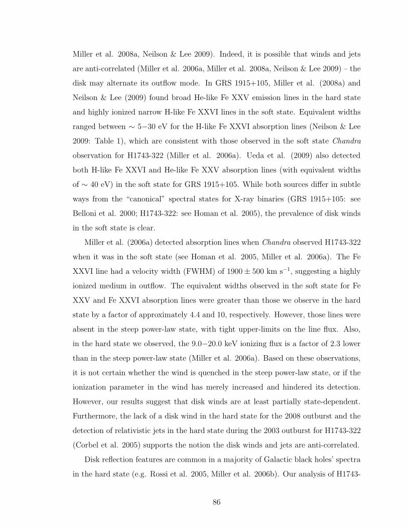
Miller et al. 2008a, Neilson & Lee 2009). Indeed, it is possible that winds and jets

are anti-correlated (Miller et al. 2006a, Miller et al. 2008a, Neilson & Lee 2009) – the

disk may alternate its outflow mode. In GRS 1915+105, Miller et al. (2008a) and

Neilson & Lee (2009) found broad He-like Fe XXV emission lines in the hard state

and highly ionized narrow H-like Fe XXVI lines in the soft state. Equivalent widths

ranged between ∼ 5−30 eV for the H-like Fe XXVI absorption lines (Neilson & Lee

2009: Table 1), which are consistent with those observed in the soft state Chandra

observation for H1743-322 (Miller et al. 2006a). Ueda et al. (2009) also detected

both H-like Fe XXVI and He-like Fe XXV absorption lines (with equivalent widths

of ∼ 40 eV) in the soft state for GRS 1915+105. While both sources differ in subtle

ways from the “canonical” spectral states for X-ray binaries (GRS 1915+105: see

Belloni et al. 2000; H1743-322: see Homan et al. 2005), the prevalence of disk winds

in the soft state is clear.

Miller et al. (2006a) detected absorption lines when Chandra observed H1743-322

when it was in the soft state (see Homan et al. 2005, Miller et al. 2006a). The Fe

XXVI line had a velocity width (FWHM) of 1900 ± 500 km s−1, suggesting a highly

ionized medium in outflow. The equivalent widths observed in the soft state for Fe

XXV and Fe XXVI absorption lines were greater than those we observe in the hard

state by a factor of approximately 4.4 and 10, respectively. However, those lines were

absent in the steep power-law state, with tight upper-limits on the line flux. Also,

in the hard state we observed, the 9.0−20.0 keV ionizing flux is a factor of 2.3 lower

than in the steep power-law state (Miller et al. 2006a). Based on these observations,

it is not certain whether the wind is quenched in the steep power-law state, or if the

ionization parameter in the wind has merely increased and hindered its detection.

However, our results suggest that disk winds are at least partially state-dependent.

Furthermore, the lack of a disk wind in the hard state for the 2008 outburst and the

detection of relativistic jets in the hard state during the 2003 outburst for H1743-322

(Corbel et al. 2005) supports the notion the disk winds and jets are anti-correlated.

Disk reflection features are common in a majority of Galactic black holes’ spectra

in the hard state (e.g. Rossi et al. 2005, Miller et al. 2006b). Our analysis of H1743-

86

322 indicates the presence of such features, most notably, the Fe Kα emission line.

The predicted equivalent widths of the Fe K emission line depend on the geometry,

inclination, and ionization state of the system. For a centrally illuminated neutral

disk with varying power-law photon index (1.3 ≤ Γ ≤ 2.3), an equivalent width

between 100 eV and 150 eV is expected for an inclination range of 45−60 degrees

(George & Fabian 1991: Figure 14) . For an ionized disk (1.0 < log ξ < 5.0, with

ξ being the ionization parameter), equivalent widths can range between 100 eV and

500 eV (Ballantyne et al. 2002: Figure 3). Note that Miller et al. (2006a) detected

no reflection features for this source in the soft state and the steep power-law state.

Based on the calculations in George & Fabian (1991), a possible explanation for our

low equivalent width values is a high inclination (i.e. θ > 80 ). Viewing the central

engine through a corona seen at high inclination can serve to diminish the clarity of

reflection features (Petrucci et al. 2001). Dips seen in the light curves for H1743-322

also indicate that it is likely viewed at a high inclination (Miller et al. 2006a: Figure

5).

Additionally, by using the width (i.e. FWHM) of the Fe K emission line we

can estimate how far the inner disk extends in H1743-322. Note that there is high

uncertainty in FWHM (0.6(3) keV), which only allows for lower and upper boundaries

of the inner disk radius. Based on our model (i.e. broken power-law added to a

Gaussian component) and given in units of gravitational radii (rg = GMBH/c2), the

inner disk ranges from ∼ 40−600rg. The innermost stable circular orbit (ISCO)

around a nonspinning black hole is rISCO = 6rg. A possible explanation for the large

differences between our estimates and the expected inner disk radius for a nonspinning

black hole is that the inner disk does not extend to the ISCO and is truncated (see

e.g. Esin et al. 1997). However, given that our estimates are inferred from parameter

values that are poorly constrained, we must regard our inferred radii with caution.

It is possible, for instance, that the detection of a red wing in a relativistic line is

prevented by calibration uncertainties in the 2.0-3.0 keV band that can have a small

impact on the continuum.

87

Parameter ValueNH(1022cm−2) 2.00(1)

Γ1 1.55(1)Γ2 2.2(1)

Ebreak (keV) 36(2)Kbnpl 0.280(3)

F0.5−200(10−9) 7.51(8)LX (0.5−200)(1037ergs−1) 6.37(7)

χ2/ ν 3053/3093

Table 4.1. Broken power-law model parameters. The results of a broadband spectral fit to theSuzaku spectra in the 0.7−200 keV band are presented above. The model is described in XSPECas tbabs x (bknpow). A constant was allowed to float between the XIS, PIN and GSO data. Thenormalization of the broken power-law component is photons cm−2s−1keV−1 at 1 keV. The fluxquoted above is an “unabsorbed” flux. The distance to H1743−322 is unknown; a Galactic centerdistance of d = 8.5 kpc was assumed to calculate the luminosity value. All errors are 90 % confidenceerrors. Errors given in parentheses are symmetric errors in the last significant digit.

Parameter ValueNH(1022cm−2) 1.98(1)

To (keV) 0.25(2)Te (keV) 38(5)

τ 1.6(2)Normalization (x 10−2) 1.9(2)

χ2/ ν 3066/3092

Table 4.2. Comptonization model parameters. The results of a broadband spectral fit to theSuzaku spectra in the 0.7−200 keV band are presented above. The model is described in XSPECas tbabs x (compTT). A constant was allowed to float between the XIS, PIN and GSO data. Theredshift was set to zero and disk geometry was assumed. Errors given in parentheses are symmetricerrors in the last significant digit.

Parameter Theoretical Value Flux W(A) (10−5 photons cm−2 s−1) (mA, eV)

Fe XXV 1.850 5.1 0.97, 3.5Fe XXVI 1.780 3.4 0.64, 2.5

Table 4.3. X-ray absorption lines upper limits. Specifically, these are parameters for the He-likeFe XXV (1s2−1s2p) and H-like Fe XXVI (1s−2p) resonance absorption lines. Since no significantlines were detected, 90% confidence upper limits are given.

88

Parameter Theoretical Value Model Value FWHM Flux W(A, keV) (keV) (keV) (10−5 photons cm−2 s−1) (mA, eV)

Low ion. Fe 1.940, 6.40 6.3(1) 0.6(3) 0.3(1) 5(2), 17(6)

Table 4.4. X-ray emission line detection. Specifically, these are parameters for low ioniza-tion iron (Fe I − Fe XVI), He-like Fe XXV and H-like Fe XXVI emission lines for the tbabs x(gaussian+bknpow) model. 90% confidence errors are given. Low ionization iron with FWHM =0.6 keV is a weak detection that resulted from allowing the line energy to vary between 6−7 keVwhile σ varied between 0 and 3 keV. Note that the line energy for low ionization iron changes only0.3 keV between those charge states, which is the reason 6.40 keV was used as the theoretical value.

89

Figure 4.1. Light curve and hardness ratio for the 2003 and 2008 outburst of H1743-322. Left panel :RXTE/ASM one-day averaged light curve with errors (1.5−12 keV) and one-day averaged (5−12keV)/(3−5 keV) hardness ratio, for the bright phase of the 2003 outburst of H1743-322 (Miller etal. 2006a). The source progresses through the steep power-law state followed by the soft state. Thearrows at the top of the plot denote the days on which H1743-322 was observed with Chandra. Rightpanel : RXTE/ASM one-day averaged light curve with errors (1.5−12 keV) and one-day averaged(5−12 keV)/(3−5 keV) hardness ratio, for the October 2008 outburst of H1743-322. The source riseis typical of the hard state. The arrow at the top of the plot denotes the date on which we observedH1743-322 with Suzaku.

90

1 10 100

0.01

0.1

110

norm

aliz

ed c

ount

s/se

c/ke

V

Energy (keV)

Figure 4.2. Suzaku spectrum of H1743-322 fitted with a broken power-law model. The curveswithin the 0.7−1.5 keV and 2.2−10.0 keV energy ranges represent the data from the XIS detectors.The curves within the 12.0−70.0 keV and 70.0−200 keV energy ranges represent the data from thePIN and GSO detectors, respectively. See also Table 1

1 10 100

0.9

11.

11.

2

ratio

Energy (keV)

Figure 4.3. Data/model ratio for the broken power-law model. The curves within the 0.7−1.5keV and 2.2−10.0 keV energy ranges represent the data from the XIS detectors. The curves withinthe 12.0−70.0 keV and 70.0−200 keV energy ranges represent the data from the PIN and GSOdetectors, respectively.

91

3 4 5 6 7 8 90.9

0.95

11.

05

ratio

Energy (keV)

Figure 4.4. Data/model ratio from 3−9 keV for the broken power-law model. The curves representthe data from the XIS detectors. There is a possible emission line around 6.4 keV.

92

CHAPTER 5

Conclusions

Throughout this thesis, we have discussed X-ray studies of three accreting compact

objects in detail with the aim of better understanding their fundamental properties,

such as black hole spin, neutron star mass and radius, and the nature of nearby

accretion flows. Using spectral models, we have analyzed Suzaku spectra of two

black hole LMXBs, GRS 1915+105 and H1743-322, and one neutron star LMXB, 4U

1636-53. We conclude by summarizing our findings from each chapter and discussing

our results in the broader context of the fundamental properties of accreting compact

objects.

5.1 Summary of Results from Individual Chapters

5.1.1 Chapter 2 Summary

Chapter 2 presents black hole spin results for GRS 1915+105, which was observed in

the hard state. Prior spin results for this source using the disk continuum method

(as opposed to using the Fe K emission line) are not consistent (i.e. McClintock et

al. 2006 and Middleton et al. 2006). Since disk reflection (and therefore the Fe K

emission line) is prominent in the spectra of this source, we fit the data using the

relativistic disk reflection models pexriv and reflionx. Our use of the Fe K emission

line method provides an independent analysis for constraining the black hole spin in

GRS 1915+105. Our results indicate that modeling nuances can be significant due to

the complex nature of the X-ray spectrum for this source. The broadband (i.e. 2.3−10

keV and 12−55 keV energy ranges) model (pexriv) suggests a maximally spinning

black hole (a = 0.98+0.01−0.01 at 1σ confidence) while the soft X-ray (< 10 keV) spectrum

93

model (reflionx) suggests a lower spin value (a = 0.56+0.02−0.02). Our broadband model

spin result is in agreement with a prior study of this source (McClintock et al. 2006),

while the upper limit on our soft X-ray spectrum model spin result is lower than the

Middleton et al. (2006) value. While a degree of uncertainty lies in our resulting spin

values (due to e.g. physical assumptions of the models, instrument calibration, etc.),

we can exclude a spin of zero at ≥ 2σ level of confidence for this source.

Black Hole Spin

Our spin results for GRS 1915+105 can further our understanding of black hole

spacetime geometry. As we have discussed, the Fe K emission line is a very useful

diagnostic of black hole spacetime and provides a means to constrain black hole spin.

Black holes (assuming that they are electrically neutral, see Blandford & Znajek

1977) can be described by two key parameters: mass and spin (and therefore angular

momentum). As such, knowing the spin is essential for understanding the physical

and dynamical properties of the compact object as a whole. For example, measuring

the black hole spin can help us to explore and confirm the Kerr metric in General

Relativity. This metric, which mathematically defines the geometry of spacetime

around a rotating black hole (i.e. for “Kerr” black hole, a6= 0), is solved when both

the black hole mass and spin are known.

Additionally, black hole spin values may be useful for understanding jet produc-

tion. Theoretically, it is possible that spin energy from a black hole can be “extracted”

and used to power the relativistic jets that have been observed in black hole LMXBs

(see e.g. Blandford & Znajek 1977). Moreover, it is certain that stellar-mass black

holes gain most of their spin (or angular momentum) when they are created (see e.g.

Volonteri et al. 2005). Thus, spin values are useful for understanding the physical

properties of the progenitor star (i.e. a massive star) as well as the dynamics of the

supernova explosion (see e.g. Heger & Woosley 2001).

Future Work

In our effort to constrain the spin of GRS 1915+105, we have considered only a single

observation in a single spectral state (i.e. the hard state), though disk reflection is sure

94

to be important in many states. Future observations with Suzaku and XMM-Newton

in different states may allow the spin to be determined more clearly using the disk

reflection spectrum. The thermal disk continuum is not evident in our observation,

but future efforts that make joint use of the direct and reflected disk spectrum to

constrain the spin (e.g. Miller et al. 2009) may provide another way forward.

5.1.2 Chapter 3 Summary

In Chapter 3 we discuss a detailed analysis of 4U 1636-53 and estimate an upper limit

on the neutron star radius using the Fe K emission line. In four of the five observa-

tions, we detect broad Fe K emission lines at greater than the 3σ level of confidence.

Due to the broadened shape of the line profile, we fit the iron lines with the diskline

model. This gives a lower limit on the inner radius of the accretion disk and thus

an upper limit on the radius of the neutron star. This severe limit corresponds to

a radius of 12 km for a 1.4 M⊙ star for our observations when the source is in the

island (transitional) state and the medium-luminosity banana (soft) state. Our inner

disk radius results from iron line fits are consistent with those from independent mea-

surements using the disk continuum and suggest that the inner disk radius may not

vary with spectral state. We fit a neutron star disk reflection model to the data for

self-consistency, but the model did not permit strong parameter constraints. More-

over, the detection of Fe K emission lines and kHz QPOs in overlapping observations

supports the notion that the iron line is indeed formed through disk reflection and

not in an optically thick disk wind; this is because such an outflow would scatter

away any variability. Additionally, we can use the upper kHz QPO frequency (which

we assume to represent the orbital frequency at the inner edge of the accretion disk)

in conjunction with our inner disk radius results to get a constraint on the mass on

M≤ 2.4M⊙ (using the equation νorb = (1/2π)√

GM/r3 and solving for M ).

Inner Disk Radius and Neutron Star Radius

Although many theories exist, the cause of spectral state transitions, which would give

us insight into the dynamical and kinematic properties of spectral state, is not well

known. Our constant values of the inner disk radius across varying spectral states for

95

4U 1636-53 would have significant implications for understanding the nature of state

transitions; that is, our results may help to determine how certain components (such

as, e.g. the mass accretion rate, M) are involved in spectral state transitions. M may

affect the extent of the inner disk radius and therefore, cause state transitions. Based

on our results, there may be a correlation between M and spectral state for this

source, but we cannot make firm conclusions since we have only observed this source

in a narrow range of spectral states. Moreover, if the inner disk does indeed remain

roughly constant, there may be no clear correlation with M . Thus, this may point

to alternative possibilities for state transitions such as a corona, boundary layer, a

magnetosphere, or a jet, and further our understanding of how such components are

involved in state transitions (van der Klis 2006, Fender 2006, Lin et al. 2010).

Getting constraints on the neutron star radius is important for understanding the

nature of ultradense matter in neutron stars. Neutron star radius and mass are the

two parameters necessary towards constraining the neutron star EOS, which describes

a neutron star’s composition (Lattimer & Prakash 2001). While our results for 4U

1636-53 have provided limits on the radius parameter, our mass estimates are too

broad to constrain the neutron star EOS.

Future Work

Future simultaneous spectral and timing observations for 4U 1636-53 can help obtain

better mass estimates and allow us to constrain the neutron star EOS. Moreover,

more observations of this source in other spectral states such as the extreme island

state and high luminosity banana state may make our conclusion regarding a constant

inner disk radius more certain.

5.1.3 Chapter 4 Summary

Chapter 4 presents results from H1743-322 in which we found no evidence of disk

winds while the source was in the hard state during its 2008 outburst. We fit the

spectra separately with phenomenological models such as a broken power-law model

and Comptonization model. Since X-ray absorption lines are indicative of disk winds,

we test for the presence of Fe XXV (6.70 keV) and Fe XXVI (6.97 keV) lines in the

96

spectra. Fitting a Gaussian component to the broken power-law model revealed that

the equivalent width upper limits for both iron absorption lines were < 3.5 eV; as

such, we conclude that these lines were not present in the spectra for H1743-322 when

it was observed in the hard state. We compare our results to those from Miller et al.

(2006a). These authors observed H1743-322 with Chandra during its 2003 outburst

when it was in the soft state and steep power-law state. Notably, Miller et al. (2006a)

detected iron absorption lines in the soft state (e.g. equivalent widths of 16(1) eV

amd 25(3) eV) but not in the steep power-law state (equivalent width upper limits <

4.3 eV). The combined results of Suzaku and Chandra indicate that there is a partial

spectral state dependence on iron absorption lines, and therefore disk winds.

Moreover, we detect a significant Fe K emission line (> 4σ level of confidence),

which is indicative of disk reflection features. These features are fairly common in

the spectra of Galactic black holes in the hard state. However, the low equivalent

width of the iron line (17(6) eV) may indicate that the source is being viewed at a

high inclination (i.e. > 80), which can smear out disk reflection features (George &

Fabian 1991, Petrucci et al. 2001).

Disk Winds and Jets

The Suzaku and Chandra results for H1743-322 suggest that disk winds are partially

state-dependent. That is, disk winds are strongest in the soft state and weak or absent

in the other states. These results support the possibility that disk winds and jets are

anti-correlated in black hole LMXBs. That is, the disk may alternate its outflow

mode for different spectral states. For example, relatvistic jets were detected in the

hard state for H1743-322 (Corbel et al. 2005) when disk winds were absent in the

same state (albeit, observations were taken for two different outbursts). Currently,

jets have never been observed in the soft state. Indeed, such a relation would have

significant consequences for disk-jet coupling. Strictly regarding the hard and soft

states, an anti-correlation between disk winds and jets could imply that black hole

LMXBs have a means of regulating their own evolution. If, for example, the same

amount of mass is lost in both the disk wind and the jets, then the source is able

97

to maintain “equilibrium in outflow”; mass lost in the outflow remains the same

regardless of the spectral state or the type of outflow (see e.g. Neilsen & Lee 2009).

Moreover, the suggestion that disk winds and jets are anti-correlated supports the

hypothesis that accretion disks are responsible for jet formation (see Sec. 1.4). That

is, a mechanism in the accretion disk allows it to change its outflow mode. Thus,

if magnetic fields in the accretion disk are responsible for jet formation, this may

support magnetically driven winds as well (see e.g. Proga et al. 2008, 2010, Miller et

al. 2008a).

Future Work

Although examining disk winds and disk reflection in black hole LMXBs can be obser-

vationally challenging, the possibility of a state-dependent anti-correlation between

winds and jets may offer insights into the dynamical properties of the accretion disk.

Moreover, such a correlation may extend from stellar-mass black holes in LMXBs

to supermassive black holes (M ∼ 106−109 M⊙) in active galactic nuclei (AGN).

Thus, this may further our understanding about the radio-loud and radio-quiet modes

of AGN (which contain supermassive black holes). The X-ray telescopes Chandra,

XMM-Newton, and Suzaku can all make important contributions in this regard.

98

BIBLIOGRAPHY

Abramowicz, M. A., Bulik, T., Bursa, M., & Kluzniak, W. 2003, A&A, 404, L21

Aitken, R. G. 1964, The binary stars, ed. Aitken, R. G.

Akmal, A., Pandharipande, V. R., & Ravenhall, D. G. 1998, Physical Review C, 58,1804

Altamirano, D., van der Klis, M., Mendez, M., Jonker, P. G., Klein-Wolt, M., &Lewin, W. H. G. 2008, ApJ, 685, 436

Arnaud, K. A. 1996, in Astronomical Society of the Pacific Conference Series, Vol.101, Astronomical Data Analysis Software and Systems V, ed. G. H. Jacoby &J. Barnes, 17–+

Asai, K., Dotani, T., Nagase, F., & Mitsuda, K. 2000, ApJS, 131, 571

Baade, W. & Zwicky, F. 1934, Physical Review, 45, 138

Balbus, S. A. & Hawley, J. F. 1991, ApJ, 376, 214

Ballantyne, D. R. 2004, MNRAS, 351, 57

Ballantyne, D. R., Fabian, A. C., & Ross, R. R. 2002, MNRAS, 329, L67

Ballantyne, D. R. & Strohmayer, T. E. 2004, ApJL, 602, L105

Bardeen, J. M., Press, W. H., & Teukolsky, S. A. 1972, ApJ, 178, 347

Barret, D. & Olive, J. 2002, ApJ, 576, 391

Barret, D., Olive, J. F., Boirin, L., Done, C., Skinner, G. K., & Grindlay, J. E. 2000,ApJ, 533, 329

Baym, G. & Pethick, C. 1975, Annual Review of Nuclear and Particle Science, 25, 27

Begelman, M. C., McKee, C. F., & Shields, G. A. 1983, ApJ, 271, 70

Belloni, T., Homan, J., Motta, S., Ratti, E., & Mendez, M. 2007, MNRAS, 379, 247

Belloni, T., Klein-Wolt, M., Mendez, M., van der Klis, M., & van Paradijs, J. 2000,A&A, 355, 271

Belloni, T., Mendez, M., & Homan, J. 2005, A&A, 437, 209

99

Bhattacharyya, S. & Strohmayer, T. E. 2007, ApJL, 664, L103

Bhattacharyya, S., Strohmayer, T. E., Miller, M. C., & Markwardt, C. B. 2005, ApJ,619, 483

Blandford, R. D. & Payne, D. G. 1982, MNRAS, 199, 883

Blandford, R. D. & Znajek, R. L. 1977, MNRAS, 179, 433

Blum, J. L., Miller, J. M., Cackett, E., Yamaoka, K., Takahashi, H., Raymond, J.,Reynolds, C. S., & Fabian, A. C. 2008, The Astronomer’s Telegram, 1841, 1

Blum, J. L., Miller, J. M., Cackett, E., Yamaoka, K., Takahashi, H., Raymond, J.,Reynolds, C. S., & Fabian, A. C. 2010, ApJ, 713, 1244

Blum, J. L., Miller, J. M., Fabian, A. C., Miller, M. C., Homan, J., van der Klis, M.,Cackett, E. M., & Reis, R. C. 2009, ApJ, 706, 60

Bogdanov, S., Rybicki, G. B., & Grindlay, J. E. 2007, ApJ, 670, 668

Brenneman, L. W. & Reynolds, C. S. 2006, ApJ, 652, 1028

Cackett, E. M., Miller, J. M., Ballantyne, D. R., Barret, D., Bhattacharyya, S.,Boutelier, M., Miller, M. C., Strohmayer, T. E., & Wijnands, R. 2010, ApJ, 720,205

Cackett, E. M., Miller, J. M., Bhattacharyya, S., Grindlay, J. E., Homan, J., van derKlis, M., Miller, M. C., Strohmayer, T. E., & Wijnands, R. 2008, ApJ, 674, 415

Cackett, E. M., Miller, J. M., Homan, J., van der Klis, M., Lewin, W. H. G., Mendez,M., Raymond, J., Steeghs, D., & Wijnands, R. 2009, ApJ, 690, 1847

Casares, J., Cornelisse, R., Steeghs, D., Charles, P. A., Hynes, R. I., O’Brien, K., &Strohmayer, T. E. 2006, MNRAS, 373, 1235

Castro-Tirado, A. J., Brandt, S., & Lund, N. 1992, IAU Circ., 5590, 2

Charles, P. A. & Coe, M. J. 2006, Optical, ultraviolet and infrared observations ofX-ray binaries, ed. Lewin, W. H. G. & van der Klis, M., 215–265

Corbel, S., Kaaret, P., Fender, R. P., Tzioumis, A. K., Tomsick, J. A., & Orosz, J. A.2005, ApJ, 632, 504

Cottam, J., Paerels, F., & Mendez, M. 2002, Nature, 420, 51

D’Aı, A., et al. 2010, A&A, 516, A36+

D’Aı, A., Iaria, R., Di Salvo, T., Matt, G., & Robba, N. R. 2009, ApJL, 693, L1

Davis, S. W., Done, C., & Blaes, O. M. 2006, ApJ, 647, 525

100

Day, C. S. R. & Done, C. 1991, MNRAS, 253, 35P

Dhawan, V., Mirabel, I. F., & Rodrıguez, L. F. 2000, ApJ, 543, 373

Dickey, J. M. & Lockman, F. J. 1990, ARA&A, 28, 215

Done, C. & Gierlinski, M. 2006, MNRAS, 367, 659

Dovciak, M., Karas, V., & Yaqoob, T. 2004, ApJS, 153, 205

Doxsey, R., et al. 1977, IAU Circ., 3113, 2

Esin, A. A., McClintock, J. E., & Narayan, R. 1997, ApJ, 489, 865

Fabian, A. C., Iwasawa, K., Reynolds, C. S., & Young, A. J. 2000, PASP, 112, 1145

Fabian, A. C. & Miniutti, G. 2009, The X-ray spectra of accreting Kerr black holes,Cambridge University Press, ed. Wiltshire, D. L., Visser, M., & Scott, S. M.

Fabian, A. C., Rees, M. J., Stella, L., & White, N. E. 1989, MNRAS, 238, 729

Fender, R. 2006, Jets from X-ray binaries, ed. Lewin, W. H. G. & van der Klis, M.,381–419

Fender, R. & Belloni, T. 2004, ARA&A, 42, 317

Fender, R. P., Garrington, S. T., McKay, D. J., Muxlow, T. W. B., Pooley, G. G.,Spencer, R. E., Stirling, A. M., & Waltman, E. B. 1999, MNRAS, 304, 865

Ford, E. C., van der Klis, M., Mendez, M., Wijnands, R., Homan, J., Jonker, P. G.,& van Paradijs, J. 2000, ApJ, 537, 368

Frank, J., King, A., & Raine, D. J. 2002, Accretion Power in Astrophysics: ThirdEdition, ed. Frank, J., King, A., & Raine, D. J.

Galloway, D. K., Psaltis, D., Muno, M. P., & Chakrabarty, D. 2006, ApJ, 639, 1033

George, I. M. & Fabian, A. C. 1991, MNRAS, 249, 352

Ghisellini, G., George, I. M., Fabian, A. C., & Done, C. 1991, MNRAS, 248, 14

Gold, T. 1968, Nature, 218, 731

Greiner, J., Cuby, J. G., McCaughrean, M. J., Castro-Tirado, A. J., & Mennickent,R. E. 2001, A&A, 373, L37

Hasinger, G. & van der Klis, M. 1989, A&A, 225, 79

Hasinger, G., van der Klis, M., Ebisawa, K., Dotani, T., & Mitsuda, K. 1990, A&A,235, 131

Heger, A. & Woosley, S. E. 2002, ApJ, 567, 532

101

Heinke, C. O., Rybicki, G. B., Narayan, R., & Grindlay, J. E. 2006, ApJ, 644, 1090

Hewish, A., Bell, S. J., Pilkington, J. D. H., Scott, P. F., & Collins, R. A. 1968,Nature, 217, 709

Ho, W. C. G., Kaplan, D. L., Chang, P., van Adelsberg, M., & Potekhin, A. Y. 2007,MNRAS, 375, 821

Homan, J., Klein-Wolt, M., Rossi, S., Miller, J. M., Wijnands, R., Belloni, T., vander Klis, M., & Lewin, W. H. G. 2003, ApJ, 586, 1262

Homan, J., Miller, J. M., Wijnands, R., van der Klis, M., Belloni, T., Steeghs, D., &Lewin, W. H. G. 2005, ApJ, 623, 383

Homan, J., et al. 2010, ApJ, 719, 201

Homan, J., et al. 2007, ApJ, 656, 420

Horowitz, C. J. & Piekarewicz, J. 2001, Physical Review Letters, 86, 5647

Inogamov, N. A. & Sunyaev, R. A. 1999, Astronomy Letters, 25, 269

Jonker, P. G., Mendez, M., & van der Klis, M. 2002, MNRAS, 336, L1

Jonker, P. G., van der Klis, M., Wijnands, R., Homan, J., van Paradijs, J., Mendez,M., Ford, E. C., Kuulkers, E., & Lamb, F. K. 2000, ApJ, 537, 374

Kallman, T. R., Palmeri, P., Bautista, M. A., Mendoza, C., & Krolik, J. H. 2004,ApJS, 155, 675

Kaluzienski, L. J. & Holt, S. S. 1977, IAU Circ., 3099, 3

Kaspi, V. M., Roberts, M. S. E., & Harding, A. K. 2006, Isolated neutron stars, ed.Lewin, W. H. G. & van der Klis, M., 279–339

Kerr, R. P. 1963, Physical Review Letters, 11, 237

King, A. R. 2006, Accretion in compact binaries, ed. Lewin, W. H. G. & van der Klis,M., 507–546

Kokubun, M., et al. 2007, PASJ, 59, 53

Kong, A. K. H., Miller, J. M., Mendez, M., Cottam, J., Lewin, W. H. G., Paerels,F., Kuulkers, E., Wijnands, R., & van der Klis, M. 2007, ApJL, 670, L17

Koyama, K., et al. 2007, PASJ, 59, 23

Kuulkers, E. & van der Klis, M. 1995, A&A, 303, 801

Lamb, F. K. & Miller, M. C. 2001, ApJ, 554, 1210

102

Laming, J. M. & Titarchuk, L. 2004, ApJL, 615, L121

Laor, A. 1991, ApJ, 376, 90

Laplace, P. S. 1795, Le Systeme du Monde, Vol. II, ed. Laplace, P. S.

Lattimer, J. M. & Prakash, M. 2001, ApJ, 550, 426

Lee, J. C., Reynolds, C. S., Remillard, R., Schulz, N. S., Blackman, E. G., & Fabian,A. C. 2002, ApJ, 567, 1102

Lin, D., Remillard, R. A., & Homan, J. 2007, ApJ, 667, 1073

Lin, D., Remillard, R. A., & Homan, J. 2009, ApJ, 696, 1257

Lin, D., Remillard, R. A., & Homan, J. 2010, ApJ, 719, 1350

Magdziarz, P. & Zdziarski, A. A. 1995, MNRAS, 273, 837

Makishima, K., Maejima, Y., Mitsuda, K., Bradt, H. V., Remillard, R. A., Tuohy,I. R., Hoshi, R., & Nakagawa, M. 1986, ApJ, 308, 635

Martocchia, A., Matt, G., Belloni, T., Feroci, M., Karas, V., & Ponti, G. 2006, A&A,448, 677

Martocchia, A., Matt, G., Karas, V., Belloni, T., & Feroci, M. 2002, A&A, 387, 215

McClintock, J. E. & Remillard, R. A. 2006, Black hole binaries, ed. Lewin, W. H. G. &van der Klis, M., 157–213

McClintock, J. E., Shafee, R., Narayan, R., Remillard, R. A., Davis, S. W., & Li, L.2006, ApJ, 652, 518

McClintok, J. E. & Remillard, R. A. 2009, in ArXiv Astrophysics e-prints, Vol. 2010,astro2010: The Astronomy and Astrophysics Decadal Survey, 197–+

Mendez, M. & Belloni, T. 2007, MNRAS, 381, 790

Merloni, A., Fabian, A. C., & Ross, R. R. 2000, MNRAS, 313, 193

Meurs, E. J. A. & van den Heuvel, E. P. J. 1989, A&A, 226, 88

Middleton, M., Done, C., Gierlinski, M., & Davis, S. W. 2006, MNRAS, 373, 1004

Migliari, S. & Fender, R. P. 2006, MNRAS, 366, 79

Miller, J. M. 2007, ARA&A, 45, 441

Miller, J. M., et al. 2010, ApJ, 724, 1441

Miller, J. M., et al. 2004, ApJL, 606, L131

103

Miller, J. M., et al. 2002, ApJ, 578, 348

Miller, J. M. & Homan, J. 2005, ApJL, 618, L107

Miller, J. M., Homan, J., & Miniutti, G. 2006c, ApJL, 652, L113

Miller, J. M., Homan, J., Steeghs, D., Rupen, M., Hunstead, R. W., Wijnands, R.,Charles, P. A., & Fabian, A. C. 2006b, ApJ, 653, 525

Miller, J. M., Raymond, J., Fabian, A., Steeghs, D., Homan, J., Reynolds, C., vander Klis, M., & Wijnands, R. 2006d, Nature, 441, 953

Miller, J. M., et al. 2006a, ApJ, 646, 394

Miller, J. M., Raymond, J., Reynolds, C. S., Fabian, A. C., Kallman, T. R., & Homan,J. 2008a, ApJ, 680, 1359

Miller, J. M., Reynolds, C. S., Fabian, A. C., Cackett, E. M., Miniutti, G., Raymond,J., Steeghs, D., Reis, R., & Homan, J. 2008b, ApJ, 679, L113

Miller, J. M., Reynolds, C. S., Fabian, A. C., Miniutti, G., & Gallo, L. C. 2009, ApJ,697, 900

Miller, J. M., Wijnands, R., Homan, J., Belloni, T., Pooley, D., Corbel, S., Kouve-liotou, C., van der Klis, M., & Lewin, W. H. G. 2001, ApJ, 563, 928

Miller, M. C., Lamb, F. K., & Psaltis, D. 1998, ApJ, 508, 791

Mirabel, I. F. & Rodrıguez, L. F. 1994, Nature, 371, 46

Mitsuda, K., et al. 2007, PASJ, 59, 1

Mitsuda, K., et al. 1984, PASJ, 36, 741

Nandra, K., George, I. M., Mushotzky, R. F., Turner, T. J., & Yaqoob, T. 1997, ApJ,477, 602

Narayan, R. & Yi, I. 1994, ApJL, 428, L13

Narayan, R. & Yi, I. 1995a, ApJ, 444, 231

Narayan, R. & Yi, I. 1995b, ApJ, 452, 710

Neilsen, J. & Lee, J. C. 2009, Nature, 458, 481

Ng, C., Dıaz Trigo, M., Cadolle Bel, M., & Migliari, S. 2010, A&A, 522, A96+

Nowak, M. A. 1995, PASP, 107, 1207

Oda, M. 1977, Space Science Reviews, 20, 757

Ohsuga, K., Mineshige, S., Mori, M., & Kato, Y. 2009, PASJ, 61, L7+

104

Ozel, F., Guver, T., & Psaltis, D. 2009, ApJ, 693, 1775

Pandel, D., Kaaret, P., & Corbel, S. 2008, ApJ, 688, 1288

Petrucci, P. O., Merloni, A., Fabian, A., Haardt, F., & Gallo, E. 2001, MNRAS, 328,501

Piraino, S., Santangelo, A., & Kaaret, P. 2000, A&A, 360, L35

Popham, R. & Sunyaev, R. 2001, ApJ, 547, 355

Pringle, J. E. 1981, ARA&A, 19, 137

Proga, D. 2003, ApJ, 585, 406

Proga, D., Stone, J. M., & Drew, J. E. 1998, MNRAS, 295, 595

Proga, D., Stone, J. M., & Kallman, T. R. 2000, ApJ, 543, 686

Psaltis, D. 2006, Accreting neutron stars and black holes: a decade of discoveries, ed.Lewin, W. H. G. & van der Klis, M., 1–38

Reis, R. C., Fabian, A. C., & Miller, J. M. 2010, MNRAS, 402, 836

Reis, R. C., Fabian, A. C., Ross, R. R., & Miller, J. M. 2009b, MNRAS, 395, 1257

Reis, R. C., Fabian, A. C., Ross, R. R., Miniutti, G., Miller, J. M., & Reynolds, C.2008, MNRAS, 387, 1489

Reis, R. C., Fabian, A. C., & Young, A. J. 2009c, MNRAS, 399, L1

Reis, R. C., Miller, J. M., & Fabian, A. C. 2009a, MNRAS, 395, L52

Remillard, R. A. & McClintock, J. E. 2006, ARA&A, 44, 49

Revnivtsev, M. G. & Gilfanov, M. R. 2006, A&A, 453, 253

Reynolds, C. S. 1997, MNRAS, 286, 513

Reynolds, C. S. & Begelman, M. C. 1997, ApJ, 488, 109

Reynolds, C. S. & Fabian, A. C. 2008, ApJ, 675, 1048

Reynolds, C. S. & Nowak, M. A. 2003, Phys. Rep, 377, 389

Ross, R. R. & Fabian, A. C. 2005, MNRAS, 358, 211

Ross, R. R., Fabian, A. C., & Young, A. J. 1999, MNRAS, 306, 461

Rossi, S., Homan, J., Miller, J. M., & Belloni, T. 2005, MNRAS, 360, 763

Rupen, M. P., Mioduszewski, A. J., & Dhawan, V. 2003, The Astronomer’s Telegram,139, 1

105

Rykoff, E. S., Cackett, E. M., & Miller, J. M. 2010, ApJ, 719, 1993

Rykoff, E. S., Miller, J. M., Steeghs, D., & Torres, M. A. P. 2007, ApJ, 666, 1129

Schwarzschild, K. 1916, Abh. Konigl. Preuss. Akad. Wissenschaften Jahre 1906,92,Berlin,1907, 189

Shafee, R., McClintock, J. E., Narayan, R., Davis, S. W., Li, L., & Remillard, R. A.2006, ApJL, 636, L113

Shafee, R., McKinney, J. C., Narayan, R., Tchekhovskoy, A., Gammie, C. F., &McClintock, J. E. 2008, ApJL, 687, L25

Shakura, N. I. & Sunyaev, R. A. 1973, A&A, 24, 337

Shapiro, S. L. & Teukolsky, S. A. 1983, Black holes, white dwarfs, and neutron stars:The physics of compact objects, ed. Shapiro, S. L. & Teukolsky, S. A.

Shaposhnikov, N., Titarchuk, L., & Laurent, P. 2009, ApJ, 699, 1223

Shih, I. C., Bird, A. J., Charles, P. A., Cornelisse, R., & Tiramani, D. 2005, MNRAS,361, 602

Shimura, T. & Takahara, F. 1995, ApJ, 445, 780

Steiner, J. F., McClintock, J. E., Remillard, R. A., Gou, L., Yamada, S., & Narayan,R. 2010, ApJL, 718, L117

Stella, L., Vietri, M., & Morsink, S. M. 1999, ApJL, 524, L63

Stirling, A. M., Spencer, R. E., de la Force, C. J., Garrett, M. A., Fender, R. P., &Ogley, R. N. 2001, MNRAS, 327, 1273

Strohmayer, T. & Bildsten, L. 2006, New views of thermonuclear bursts, ed. Lewin,W. H. G. & van der Klis, M., 113–156

Strohmayer, T. E. 2001a, ApJL, 552, L49

Strohmayer, T. E. 2001b, ApJL, 554, L169

Strohmayer, T. E. & Brown, E. F. 2002, ApJ, 566, 1045

Strohmayer, T. E. & Markwardt, C. B. 2002, ApJ, 577, 337

Swank, J. H., Becker, R. H., Boldt, E. A., Holt, S. S., Pravdo, S. H., & Serlemitsos,P. J. 1977, ApJL, 212, L73

Syunyaev, R. A. & Shakura, N. I. 1986, Soviet Astronomy Letters, 12, 117

Takahashi, T., et al. 2007, PASJ, 59, 35

106

Tananbaum, H., Gursky, H., Kellogg, E., Giacconi, R., & Jones, C. 1972, ApJL, 177,L5+

Tauris, T. M. & van den Heuvel, E. P. J. 2006, Formation and evolution of compactstellar X-ray sources, ed. Lewin, W. H. G. & van der Klis, M., 623–665

Thorne, K. S. 1974, ApJ, 191, 507

Titarchuk, L. 1994, ApJ, 434, 570

Titarchuk, L. 2002, ApJL, 578, L71

Titarchuk, L., Laurent, P., & Shaposhnikov, N. 2009, ApJ, 700, 1831

Tomsick, J. A., Kalemci, E., Kaaret, P., Markoff, S., Corbel, S., Migliari, S., Fender,R., Bailyn, C. D., & Buxton, M. M. 2008, ApJ, 680, 593

Ueda, Y., Yamaoka, K., & Remillard, R. 2009, ApJ, 695, 888

van der Klis, M. 2006, Rapid X-ray Variability, ed. Lewin, W. H. G. & van der Klis,M., 39–112

van der Klis, M., Wijnands, R. A. D., Horne, K., & Chen, W. 1997, ApJL, 481, L97+

van Paradijs, J. & Lewin, W. H. G. 1987, A&A, 172, L20

van Paradijs, J., et al. 1990, A&A, 234, 181

van Straaten, S., van der Klis, M., & Mendez, M. 2003, ApJ, 596, 1155

Volonteri, M., Madau, P., Quataert, E., & Rees, M. J. 2005, ApJ, 620, 69

White, N. E. & Marshall, F. E. 1984, ApJ, 281, 354

White, N. E., Peacock, A., Hasinger, G., Mason, K. O., Manzo, G., Taylor, B. G., &Branduardi-Raymont, G. 1986, MNRAS, 218, 129

White, N. E., Stella, L., & Parmar, A. N. 1988, ApJ, 324, 363

Wijnands, R. A. D., van der Klis, M., van Paradijs, J., Lewin, W. H. G., Lamb, F. K.,Vaughan, B., & Kuulkers, E. 1997, ApJL, 479, L141+

Wilms, J., Allen, A., & McCray, R. 2000, ApJ, 542, 914

Zhang, W., Lapidus, I., White, N. E., & Titarchuk, L. 1996, ApJL, 469, L17+

Zimmerman, E. R., Narayan, R., McClintock, J. E., & Miller, J. M. 2005, ApJ, 618,832

107