Embed Size (px)
Citation preview
Convex OptimizationFundamentals and Applications in Statistical Signal
Processing
João Mota
EURASIP/UDRC Summer School 2019
Heriot-Watt University
1-1
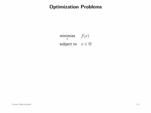
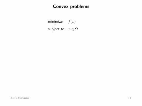
Optimization Problems
minimizex
f(x)
subject to x ∈ Ω
• x ∈ Rn: optimization variable
• f : Rn → R: cost function (or objective)
• Ω ⊂ Rn: constraint set
Convex Optimization 1-1
Optimization Problems
minimizex
f(x)
subject to x ∈ Ω
• x ∈ Rn: optimization variable
• f : Rn → R: cost function (or objective)
• Ω ⊂ Rn: constraint set
Convex Optimization 1-1
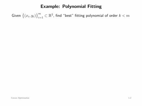
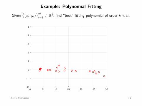
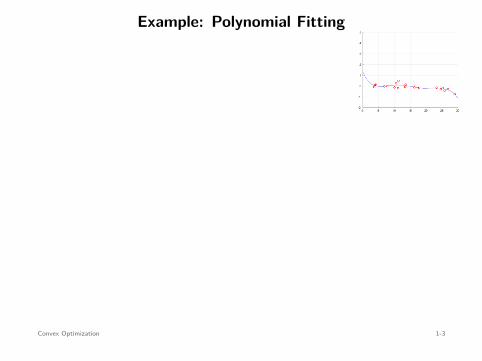
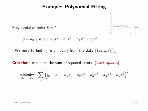
Example: Polynomial Fitting
Given
(xi, yi)m
i=1 ⊂ R2, find “best” fitting polynomial of order k < m
(xi, yi)
a0 + a1x + a2x2 + a3x3 + a4x4 + a5x5
Convex Optimization 1-2
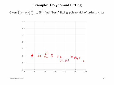
Example: Polynomial Fitting
Given
(xi, yi)m
i=1 ⊂ R2, find “best” fitting polynomial of order k < m
(xi, yi)
a0 + a1x + a2x2 + a3x3 + a4x4 + a5x5
Convex Optimization 1-2
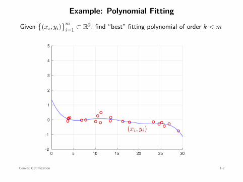
Example: Polynomial Fitting
Given
(xi, yi)m
i=1 ⊂ R2, find “best” fitting polynomial of order k < m
(xi, yi)
a0 + a1x + a2x2 + a3x3 + a4x4 + a5x5
Convex Optimization 1-2
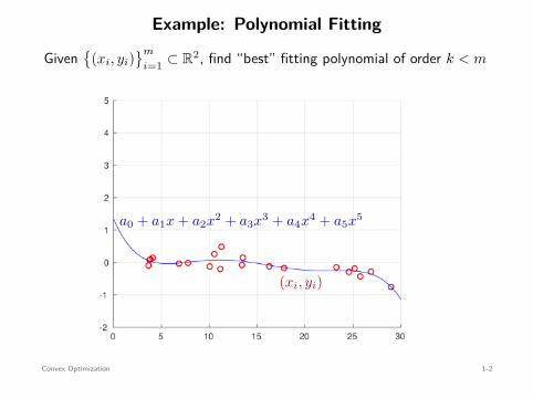
Example: Polynomial Fitting
Given
(xi, yi)m
i=1 ⊂ R2, find “best” fitting polynomial of order k < m
(xi, yi)
a0 + a1x + a2x2 + a3x3 + a4x4 + a5x5
Convex Optimization 1-2
Example: Polynomial Fitting
Given
(xi, yi)m
i=1 ⊂ R2, find “best” fitting polynomial of order k < m
(xi, yi)
a0 + a1x + a2x2 + a3x3 + a4x4 + a5x5
Convex Optimization 1-2
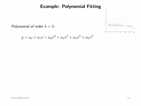
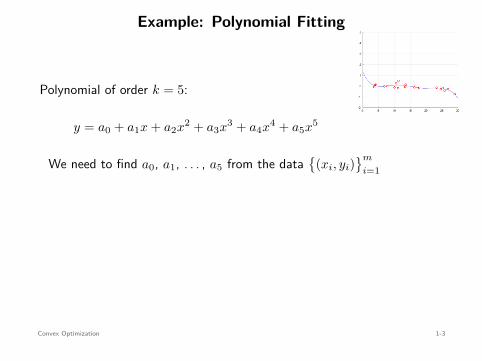
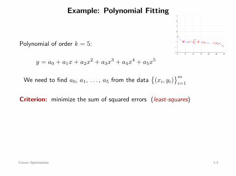
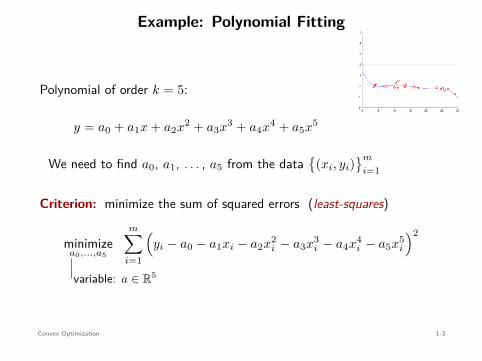
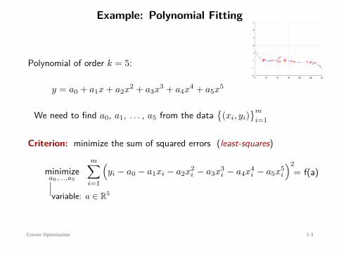
Example: Polynomial Fitting
Polynomial of order k = 5:
y = a0 + a1x + a2x2 + a3x3 + a4x4 + a5x5
We need to find a0, a1, . . . , a5 from the data
(xi, yi)m
i=1
Criterion: minimize the sum of squared errors (least-squares)
minimizea0,...,a5
m∑
i=1
(yi − a0 − a1xi − a2x2
i − a3x3i − a4x4
i − a5x5i
)2
variable: a ∈ R5
= f(a)
Convex Optimization 1-3
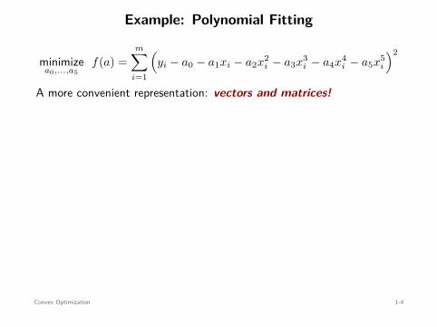
Example: Polynomial Fitting
minimizea0,...,a5
f(a) =m∑
i=1
(yi − a0 − a1xi − a2x2
i − a3x3i − a4x4
i − a5x5i
)2
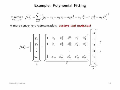
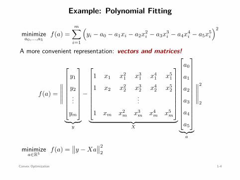
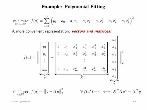
A more convenient representation: vectors and matrices!
f(a) =∥∥∥∥∥
y1
y2...
ym
︸ ︷︷ ︸y
−
1 x1 x21 x3
1 x41 x5
1
1 x2 x22 x3
2 x42 x5
2...
1 xm x2m x3
m x4m x5
m
︸ ︷︷ ︸X
a0
a1
a2
a3
a4
a5
︸ ︷︷ ︸a
∥∥∥∥∥
2
2
minimizea∈R5
f(a) =∥∥y − Xa
∥∥22
∇f(a⋆) = 0 ⇐⇒ X⊤Xa⋆ = X⊤y
Convex Optimization 1-4
Example: Polynomial Fitting
minimizea0,...,a5
f(a) =m∑
i=1
(yi − a0 − a1xi − a2x2
i − a3x3i − a4x4
i − a5x5i
)2
A more convenient representation: vectors and matrices!
f(a) =∥∥∥∥∥
y1
y2...
ym
︸ ︷︷ ︸y
−
1 x1 x21 x3
1 x41 x5
1
1 x2 x22 x3
2 x42 x5
2...
1 xm x2m x3
m x4m x5
m
︸ ︷︷ ︸X
a0
a1
a2
a3
a4
a5
︸ ︷︷ ︸a
∥∥∥∥∥
2
2
minimizea∈R5
f(a) =∥∥y − Xa
∥∥22 ∇f(a⋆) = 0 ⇐⇒ X⊤Xa⋆ = X⊤y
Convex Optimization 1-4
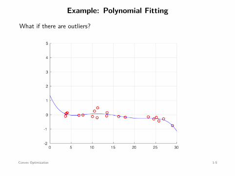
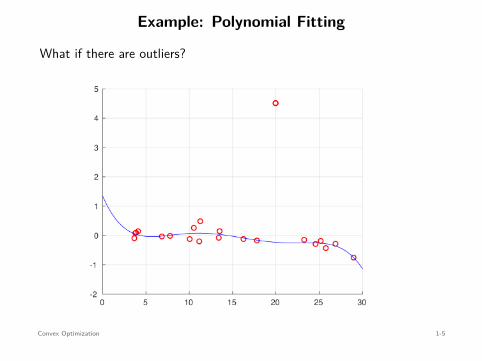
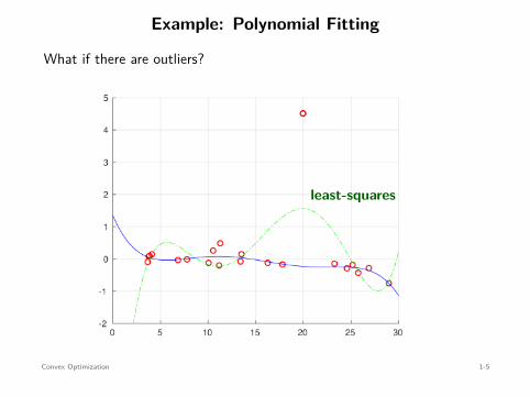
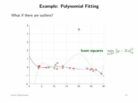
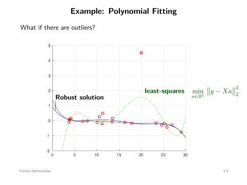
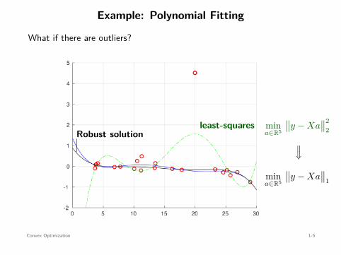
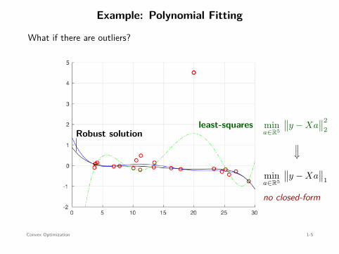
Example: Polynomial Fitting
What if there are outliers?
least-squares mina∈R5
∥∥y − Xa∥∥2
2Robust solution
⇐=
mina∈R5
∥∥y − Xa∥∥
1
no closed-form
Convex Optimization 1-5
Example: Polynomial Fitting
What if there are outliers?
least-squares mina∈R5
∥∥y − Xa∥∥2
2Robust solution
⇐=
mina∈R5
∥∥y − Xa∥∥
1
no closed-form
Convex Optimization 1-5
Example: Polynomial Fitting
What if there are outliers?
least-squares mina∈R5
∥∥y − Xa∥∥2
2Robust solution
⇐=
mina∈R5
∥∥y − Xa∥∥
1
no closed-form
Convex Optimization 1-5
Example: Polynomial Fitting
What if there are outliers?
least-squares
mina∈R5
∥∥y − Xa∥∥2
2Robust solution
⇐=
mina∈R5
∥∥y − Xa∥∥
1
no closed-form
Convex Optimization 1-5
Example: Polynomial Fitting
What if there are outliers?
least-squares mina∈R5
∥∥y − Xa∥∥2
2
Robust solution
⇐=
mina∈R5
∥∥y − Xa∥∥
1
no closed-form
Convex Optimization 1-5
Example: Polynomial Fitting
What if there are outliers?
least-squares mina∈R5
∥∥y − Xa∥∥2
2Robust solution
⇐=
mina∈R5
∥∥y − Xa∥∥
1
no closed-form
Convex Optimization 1-5
Example: Polynomial Fitting
What if there are outliers?
least-squares mina∈R5
∥∥y − Xa∥∥2
2Robust solution
⇐=
mina∈R5
∥∥y − Xa∥∥
1
no closed-form
Convex Optimization 1-5
Example: Polynomial Fitting
What if there are outliers?
least-squares mina∈R5
∥∥y − Xa∥∥2
2Robust solution
⇐=
mina∈R5
∥∥y − Xa∥∥
1
no closed-form
Convex Optimization 1-5

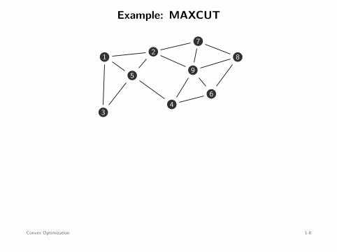
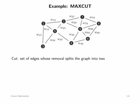
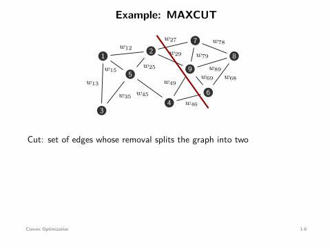
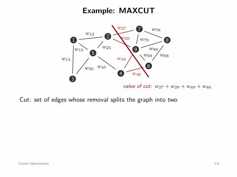
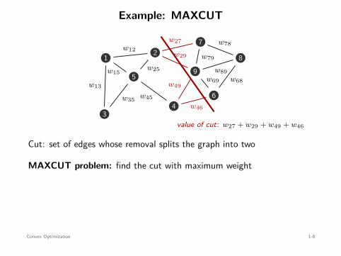
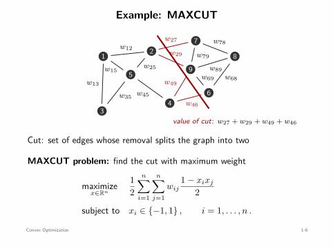
Example: MAXCUT
1 2
34
5
6
7
89
w12
w13
w15w25
w35 w45
w69 w68
w78
w79
w89
w27
w29
w49
w46
w27
w29
w49
w46
value of cut: w27 + w29 + w49 + w46
Cut: set of edges whose removal splits the graph into two
MAXCUT problem: find the cut with maximum weight
maximizex∈Rn
12
n∑
i=1
n∑
j=1wij
1 − xixj
2
subject to xi ∈ −1, 1 , i = 1, . . . , n .
Convex Optimization 1-6
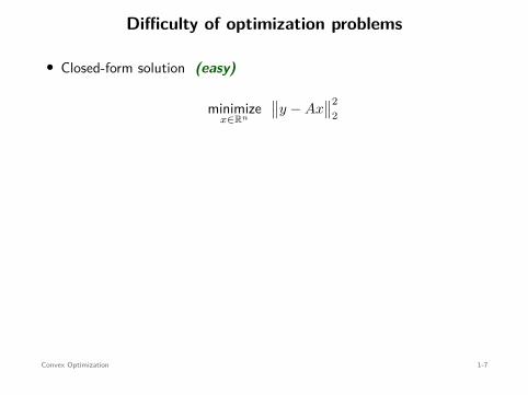
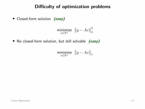
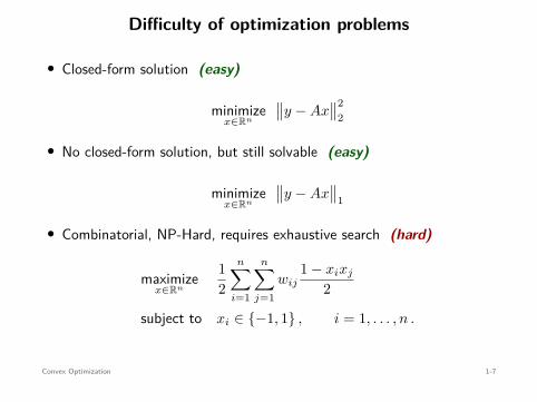
Difficulty of optimization problems
• Closed-form solution (easy)
minimizex∈Rn
∥∥y − Ax∥∥2
2
• No closed-form solution, but still solvable (easy)
minimizex∈Rn
∥∥y − Ax∥∥
1
• Combinatorial, NP-Hard, requires exhaustive search (hard)
maximizex∈Rn
12
n∑
i=1
n∑
j=1wij
1 − xixj
2
subject to xi ∈ −1, 1 , i = 1, . . . , n .
Convex Optimization 1-7
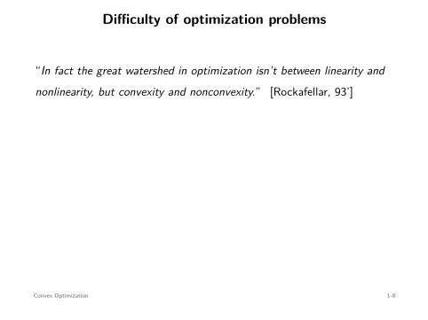
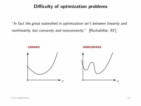
Difficulty of optimization problems
“In fact the great watershed in optimization isn’t between linearity andnonlinearity, but convexity and nonconvexity.” [Rockafellar, 93’]
x x
convex nonconvex
Convex Optimization 1-8
Difficulty of optimization problems
“In fact the great watershed in optimization isn’t between linearity andnonlinearity, but convexity and nonconvexity.” [Rockafellar, 93’]
x x
convex nonconvex
Convex Optimization 1-8

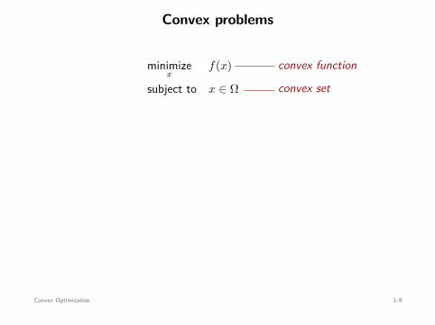
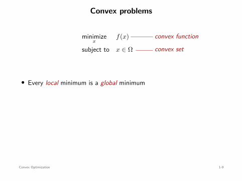
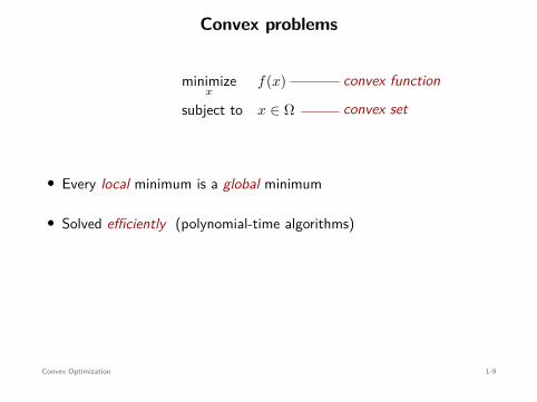
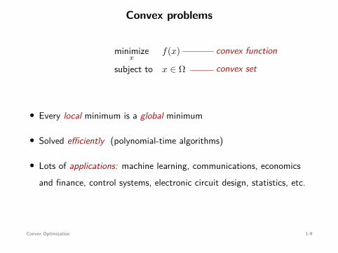
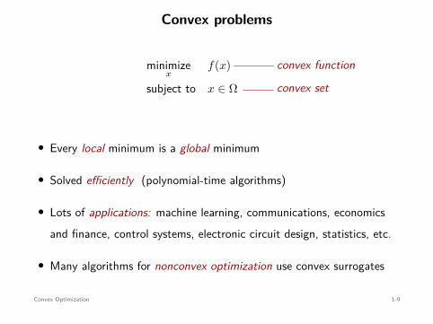
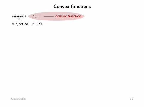
Convex problems
minimizex
f(x)
subject to x ∈ Ω
convex function
convex set
• Every local minimum is a global minimum
• Solved efficiently (polynomial-time algorithms)
• Lots of applications: machine learning, communications, economicsand finance, control systems, electronic circuit design, statistics, etc.
• Many algorithms for nonconvex optimization use convex surrogates
Convex Optimization 1-9
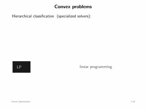
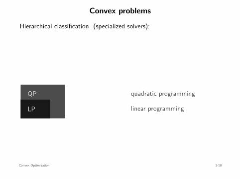
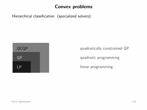
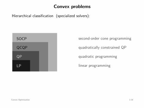
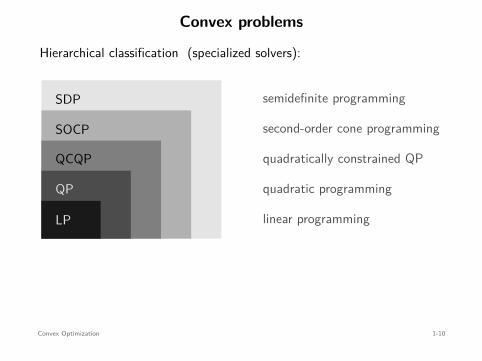
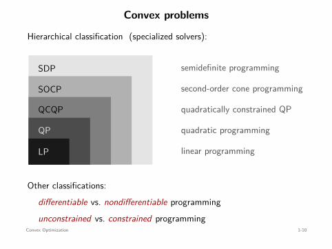
Convex problems
Hierarchical classification (specialized solvers):
LP
QP
QCQP
SOCP
SDP
linear programming
quadratic programming
quadratically constrained QP
second-order cone programming
semidefinite programming
Other classifications:differentiable vs. nondifferentiable programmingunconstrained vs. constrained programming
Convex Optimization 1-10
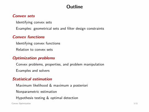
Outline
Convex setsIdentifying convex setsExamples: geometrical sets and filter design constraints
Convex functionsIdentifying convex functionsRelation to convex sets
Optimization problemsConvex problems, properties, and problem manipulationExamples and solvers
Statistical estimationMaximum likelihood & maximum a posterioriNonparametric estimationHypothesis testing & optimal detection
Convex Optimization 1-11

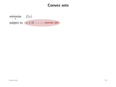
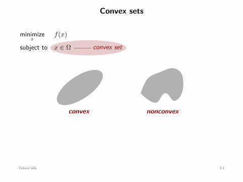
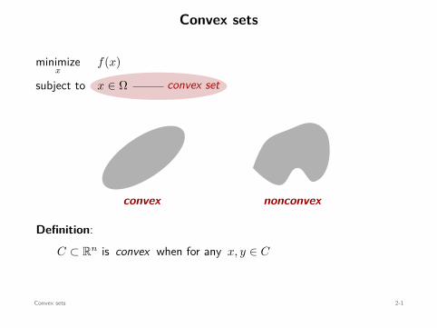
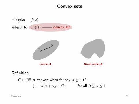
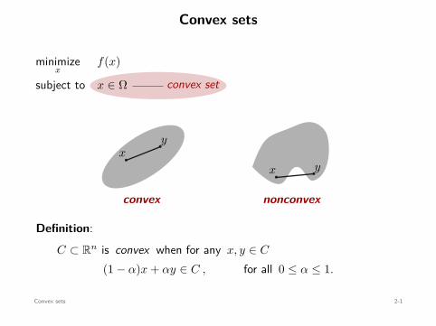
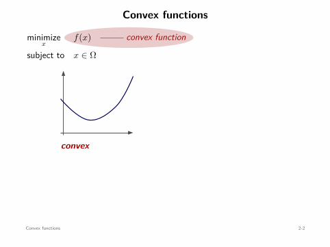
Convex sets
convex set
minimizex
f(x)
subject to x ∈ Ω
xy
convex
x y
nonconvex
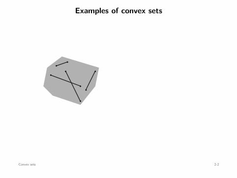
Definition:C ⊂ Rn is convex when for any x, y ∈ C
(1 − α)x + αy ∈ C , for all 0 ≤ α ≤ 1.
Convex sets 2-1
Convex sets
convex set
minimizex
f(x)
subject to x ∈ Ω
xy
convex
x y
nonconvex
Definition:C ⊂ Rn is convex when for any x, y ∈ C
(1 − α)x + αy ∈ C , for all 0 ≤ α ≤ 1.
Convex sets 2-1
Convex sets
convex set
minimizex
f(x)
subject to x ∈ Ω
xy
convex
x y
nonconvex
Definition:C ⊂ Rn is convex when for any x, y ∈ C
(1 − α)x + αy ∈ C , for all 0 ≤ α ≤ 1.
Convex sets 2-1
Convex sets
convex set
minimizex
f(x)
subject to x ∈ Ω
xy
convex
x y
nonconvex
Definition:C ⊂ Rn is convex when for any x, y ∈ C
(1 − α)x + αy ∈ C , for all 0 ≤ α ≤ 1.
Convex sets 2-1
Convex sets
convex set
minimizex
f(x)
subject to x ∈ Ω
xy
convex
x y
nonconvex
Definition:C ⊂ Rn is convex when for any x, y ∈ C
(1 − α)x + αy ∈ C , for all 0 ≤ α ≤ 1.
Convex sets 2-1

Convex sets
convex set
minimizex
f(x)
subject to x ∈ Ω
xy
convex
x y
nonconvex
Definition:C ⊂ Rn is convex when for any x, y ∈ C
(1 − α)x + αy ∈ C , for all 0 ≤ α ≤ 1.
Convex sets 2-1

Convex sets
convex set
minimizex
f(x)
subject to x ∈ Ω
xy
convex
x y
nonconvex
Definition:C ⊂ Rn is convex when for any x, y ∈ C
(1 − α)x + αy ∈ C , for all 0 ≤ α ≤ 1.
Convex sets 2-1
Convex sets
convex set
minimizex
f(x)
subject to x ∈ Ω
xy
convex
x y
nonconvex
Definition:C ⊂ Rn is convex when for any x, y ∈ C
(1 − α)x + αy ∈ C , for all 0 ≤ α ≤ 1.
Convex sets 2-1

Convex sets
convex set
minimizex
f(x)
subject to x ∈ Ω
xy
convex
x y
nonconvex
Definition:C ⊂ Rn is convex when for any x, y ∈ C
(1 − α)x + αy ∈ C , for all 0 ≤ α ≤ 1.
Convex sets 2-1
Convex sets
convex set
minimizex
f(x)
subject to x ∈ Ω
xy
convex
x y
nonconvex
Definition:C ⊂ Rn is convex when for any x, y ∈ C
(1 − α)x + αy ∈ C , for all 0 ≤ α ≤ 1.
Convex sets 2-1
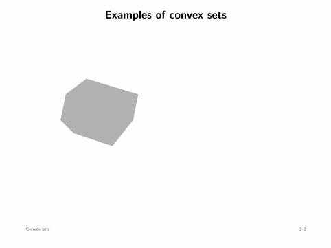
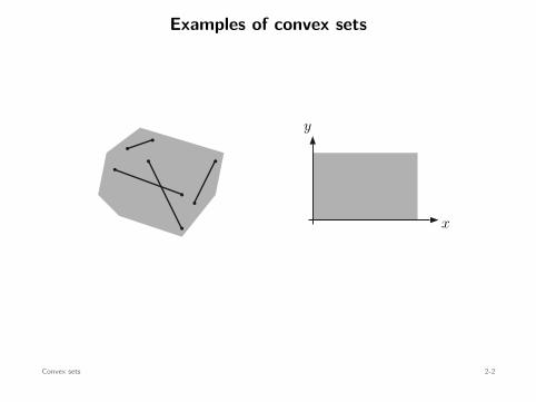
Examples of convex sets
x
y
Convex sets 2-2
Examples of convex sets
x
y
Convex sets 2-2
Examples of convex sets
x
y
Convex sets 2-2
Examples of convex sets
x
y
Convex sets 2-2

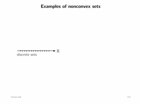
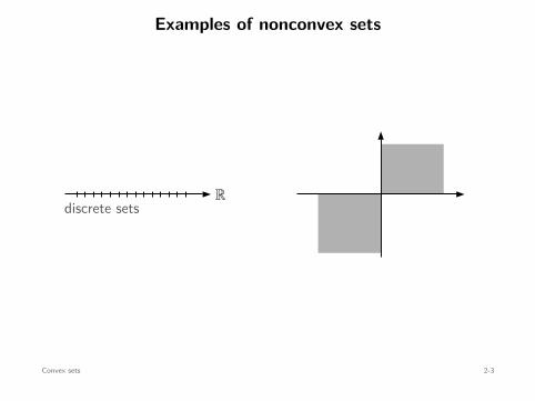
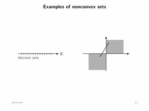
Examples of nonconvex sets
Rdiscrete sets
Convex sets 2-3
Examples of nonconvex sets
Rdiscrete sets
Convex sets 2-3
Examples of nonconvex sets
Rdiscrete sets
Convex sets 2-3
Examples of nonconvex sets
Rdiscrete sets
Convex sets 2-3

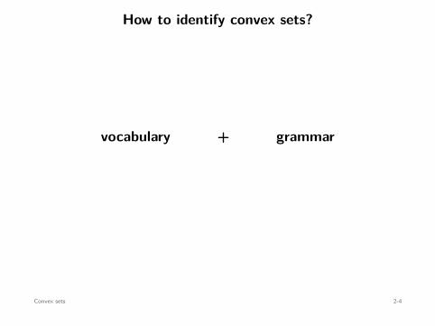
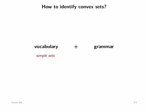
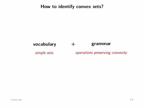
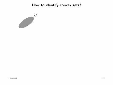
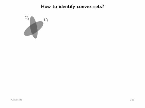
How to identify convex sets?
vocabulary + grammar
simple sets operations preserving convexity
Convex sets 2-4
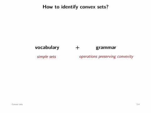
How to identify convex sets?
vocabulary + grammar
simple sets operations preserving convexity
Convex sets 2-4
How to identify convex sets?
vocabulary + grammar
simple sets
operations preserving convexity
Convex sets 2-4
How to identify convex sets?
vocabulary + grammar
simple sets operations preserving convexity
Convex sets 2-4

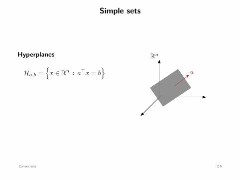
Simple sets
Hyperplanes
Ha,b =
x ∈ Rn : a⊤x = b
Rn
a
Convex sets 2-5

Simple sets
Hyperplanes
Ha,b =
x ∈ Rn : a⊤x = b
Rn
a
Convex sets 2-5
Simple sets
Hyperplanes
Ha,b =
x ∈ Rn : a⊤x = b
Rn
a
Convex sets 2-5

Simple sets
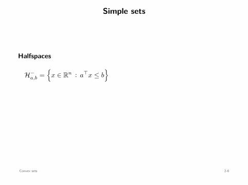
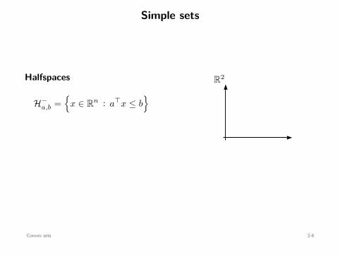
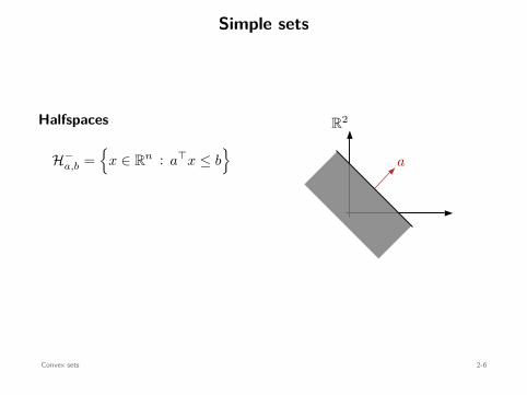
Halfspaces
H−a,b =
x ∈ Rn : a⊤x ≤ b
R2
a
Convex sets 2-6
Simple sets
Halfspaces
H−a,b =
x ∈ Rn : a⊤x ≤ b
R2
a
Convex sets 2-6
Simple sets
Halfspaces
H−a,b =
x ∈ Rn : a⊤x ≤ b
R2
a
Convex sets 2-6
Simple sets
Halfspaces
H−a,b =
x ∈ Rn : a⊤x ≤ b
R2
a
Convex sets 2-6

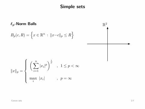
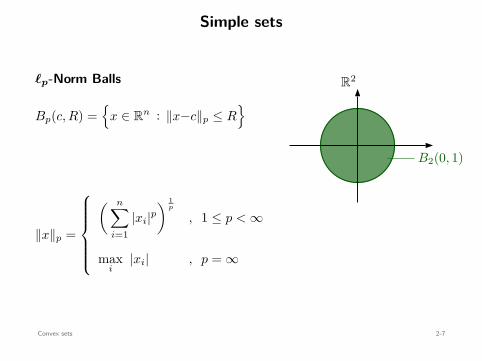
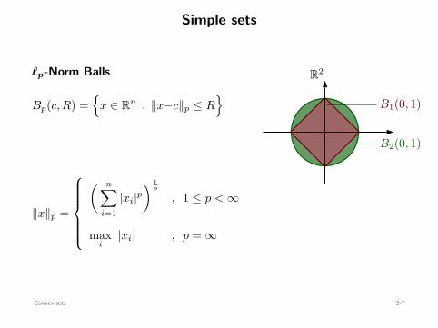
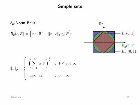
Simple sets
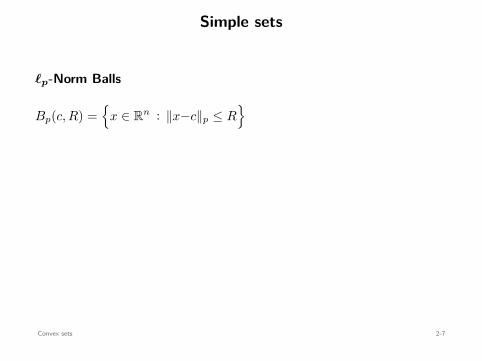
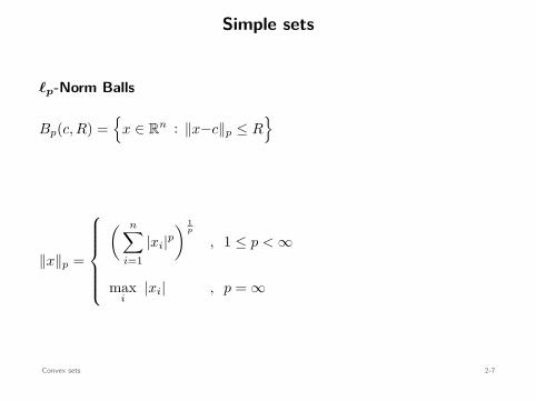
ℓp-Norm Balls
Bp(c, R) =
x ∈ Rn : ∥x−c∥p ≤ R
∥x∥p =
( n∑
i=1|xi|p
) 1p
, 1 ≤ p < ∞
maxi
|xi| , p = ∞
B∞(0, 1)B2(0, 1)
B1(0, 1)
R2
Convex sets 2-7
Simple sets
ℓp-Norm Balls
Bp(c, R) =
x ∈ Rn : ∥x−c∥p ≤ R
∥x∥p =
( n∑
i=1|xi|p
) 1p
, 1 ≤ p < ∞
maxi
|xi| , p = ∞
B∞(0, 1)B2(0, 1)
B1(0, 1)
R2
Convex sets 2-7
Simple sets
ℓp-Norm Balls
Bp(c, R) =
x ∈ Rn : ∥x−c∥p ≤ R
∥x∥p =
( n∑
i=1|xi|p
) 1p
, 1 ≤ p < ∞
maxi
|xi| , p = ∞
B∞(0, 1)B2(0, 1)
B1(0, 1)
R2
Convex sets 2-7
Simple sets
ℓp-Norm Balls
Bp(c, R) =
x ∈ Rn : ∥x−c∥p ≤ R
∥x∥p =
( n∑
i=1|xi|p
) 1p
, 1 ≤ p < ∞
maxi
|xi| , p = ∞
B∞(0, 1)B2(0, 1)
B1(0, 1)
R2
Convex sets 2-7
Simple sets
ℓp-Norm Balls
Bp(c, R) =
x ∈ Rn : ∥x−c∥p ≤ R
∥x∥p =
( n∑
i=1|xi|p
) 1p
, 1 ≤ p < ∞
maxi
|xi| , p = ∞
B∞(0, 1)
B2(0, 1)
B1(0, 1)
R2
Convex sets 2-7
Simple sets
ℓp-Norm Balls
Bp(c, R) =
x ∈ Rn : ∥x−c∥p ≤ R
∥x∥p =
( n∑
i=1|xi|p
) 1p
, 1 ≤ p < ∞
maxi
|xi| , p = ∞
B∞(0, 1)
B2(0, 1)
B1(0, 1)
R2
Convex sets 2-7
Simple sets
ℓp-Norm Balls
Bp(c, R) =
x ∈ Rn : ∥x−c∥p ≤ R
∥x∥p =
( n∑
i=1|xi|p
) 1p
, 1 ≤ p < ∞
maxi
|xi| , p = ∞
B∞(0, 1)B2(0, 1)
B1(0, 1)
R2
Convex sets 2-7
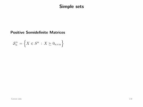
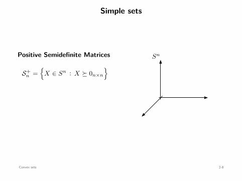
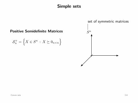
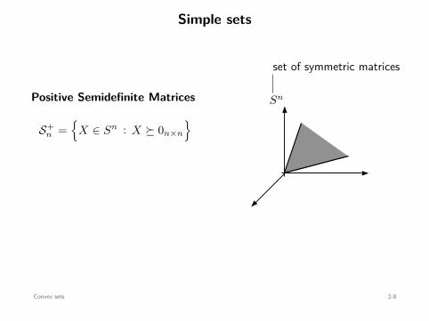
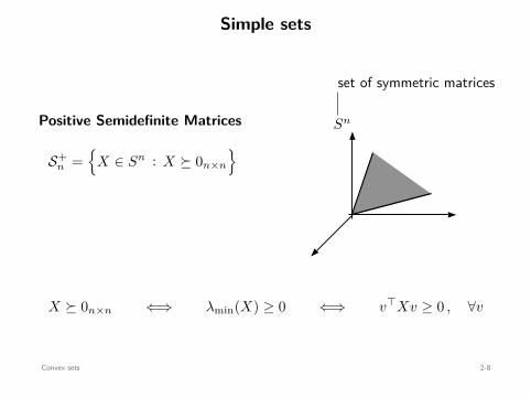
Simple sets
Positive Semidefinite Matrices
S+n =
X ∈ Sn : X ⪰ 0n×n
Sn
set of symmetric matrices
X ⪰ 0n×n ⇐⇒ λmin(X) ≥ 0 ⇐⇒ v⊤Xv ≥ 0 , ∀v
Convex sets 2-8
Simple sets
Positive Semidefinite Matrices
S+n =
X ∈ Sn : X ⪰ 0n×n
Sn
set of symmetric matrices
X ⪰ 0n×n ⇐⇒ λmin(X) ≥ 0 ⇐⇒ v⊤Xv ≥ 0 , ∀v
Convex sets 2-8
Simple sets
Positive Semidefinite Matrices
S+n =
X ∈ Sn : X ⪰ 0n×n
Sn
set of symmetric matrices
X ⪰ 0n×n ⇐⇒ λmin(X) ≥ 0 ⇐⇒ v⊤Xv ≥ 0 , ∀v
Convex sets 2-8
Simple sets
Positive Semidefinite Matrices
S+n =
X ∈ Sn : X ⪰ 0n×n
Sn
set of symmetric matrices
X ⪰ 0n×n ⇐⇒ λmin(X) ≥ 0 ⇐⇒ v⊤Xv ≥ 0 , ∀v
Convex sets 2-8
Simple sets
Positive Semidefinite Matrices
S+n =
X ∈ Sn : X ⪰ 0n×n
Sn
set of symmetric matrices
X ⪰ 0n×n ⇐⇒ λmin(X) ≥ 0 ⇐⇒ v⊤Xv ≥ 0 , ∀v
Convex sets 2-8
Simple sets
Positive Semidefinite Matrices
S+n =
X ∈ Sn : X ⪰ 0n×n
Sn
set of symmetric matrices
X ⪰ 0n×n ⇐⇒ λmin(X) ≥ 0 ⇐⇒ v⊤Xv ≥ 0 , ∀v
Convex sets 2-8
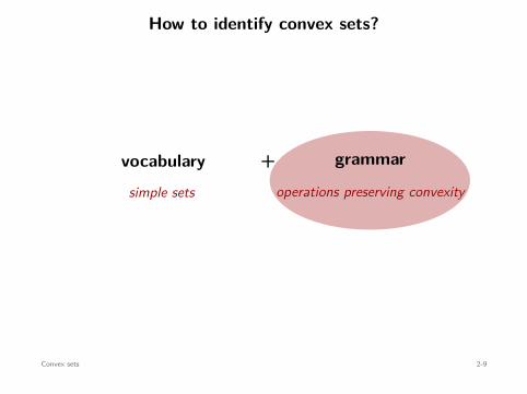
How to identify convex sets?
simple sets operations preserving convexity
vocabulary + grammar
Convex sets 2-9
How to identify convex sets?
simple sets operations preserving convexity
vocabulary + grammar
Convex sets 2-9

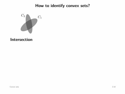
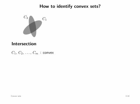
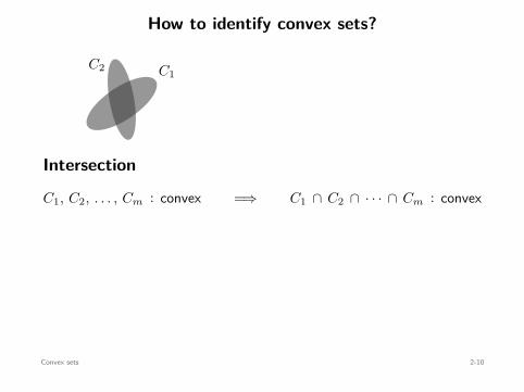
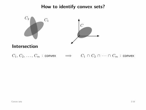
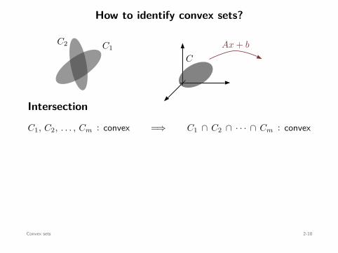
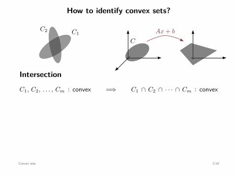
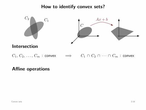
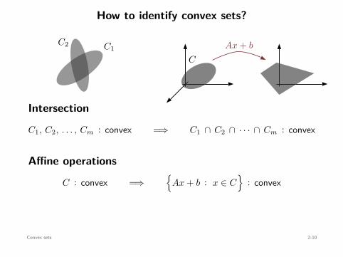
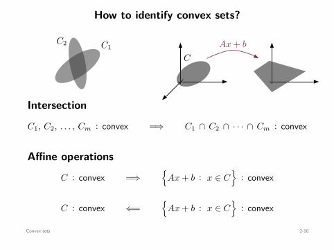
How to identify convex sets?
C1C2
C
Ax + b
Intersection
C1, C2, . . . , Cm : convex =⇒ C1 ∩ C2 ∩ · · · ∩ Cm : convex
Affine operations
C : convex =⇒
Ax + b : x ∈ C
: convex
C : convex ⇐=
Ax + b : x ∈ C
: convex
Convex sets 2-10
How to identify convex sets?
C1
C2
C
Ax + b
Intersection
C1, C2, . . . , Cm : convex =⇒ C1 ∩ C2 ∩ · · · ∩ Cm : convex
Affine operations
C : convex =⇒
Ax + b : x ∈ C
: convex
C : convex ⇐=
Ax + b : x ∈ C
: convex
Convex sets 2-10
How to identify convex sets?
C1C2
C
Ax + b
Intersection
C1, C2, . . . , Cm : convex =⇒ C1 ∩ C2 ∩ · · · ∩ Cm : convex
Affine operations
C : convex =⇒
Ax + b : x ∈ C
: convex
C : convex ⇐=
Ax + b : x ∈ C
: convex
Convex sets 2-10
How to identify convex sets?
C1C2
C
Ax + b
Intersection
C1, C2, . . . , Cm : convex =⇒ C1 ∩ C2 ∩ · · · ∩ Cm : convex
Affine operations
C : convex =⇒
Ax + b : x ∈ C
: convex
C : convex ⇐=
Ax + b : x ∈ C
: convex
Convex sets 2-10
How to identify convex sets?
C1C2
C
Ax + b
Intersection
C1, C2, . . . , Cm : convex
=⇒ C1 ∩ C2 ∩ · · · ∩ Cm : convex
Affine operations
C : convex =⇒
Ax + b : x ∈ C
: convex
C : convex ⇐=
Ax + b : x ∈ C
: convex
Convex sets 2-10
How to identify convex sets?
C1C2
C
Ax + b
Intersection
C1, C2, . . . , Cm : convex =⇒ C1 ∩ C2 ∩ · · · ∩ Cm : convex
Affine operations
C : convex =⇒
Ax + b : x ∈ C
: convex
C : convex ⇐=
Ax + b : x ∈ C
: convex
Convex sets 2-10
How to identify convex sets?
C1C2
C
Ax + b
Intersection
C1, C2, . . . , Cm : convex =⇒ C1 ∩ C2 ∩ · · · ∩ Cm : convex
Affine operations
C : convex =⇒
Ax + b : x ∈ C
: convex
C : convex ⇐=
Ax + b : x ∈ C
: convex
Convex sets 2-10
How to identify convex sets?
C1C2
C
Ax + b
Intersection
C1, C2, . . . , Cm : convex =⇒ C1 ∩ C2 ∩ · · · ∩ Cm : convex
Affine operations
C : convex =⇒
Ax + b : x ∈ C
: convex
C : convex ⇐=
Ax + b : x ∈ C
: convex
Convex sets 2-10
How to identify convex sets?
C1C2
C
Ax + b
Intersection
C1, C2, . . . , Cm : convex =⇒ C1 ∩ C2 ∩ · · · ∩ Cm : convex
Affine operations
C : convex =⇒
Ax + b : x ∈ C
: convex
C : convex ⇐=
Ax + b : x ∈ C
: convex
Convex sets 2-10
How to identify convex sets?
C1C2
C
Ax + b
Intersection
C1, C2, . . . , Cm : convex =⇒ C1 ∩ C2 ∩ · · · ∩ Cm : convex
Affine operations
C : convex =⇒
Ax + b : x ∈ C
: convex
C : convex ⇐=
Ax + b : x ∈ C
: convex
Convex sets 2-10
How to identify convex sets?
C1C2
C
Ax + b
Intersection
C1, C2, . . . , Cm : convex =⇒ C1 ∩ C2 ∩ · · · ∩ Cm : convex
Affine operations
C : convex =⇒
Ax + b : x ∈ C
: convex
C : convex ⇐=
Ax + b : x ∈ C
: convex
Convex sets 2-10
How to identify convex sets?
C1C2
C
Ax + b
Intersection
C1, C2, . . . , Cm : convex =⇒ C1 ∩ C2 ∩ · · · ∩ Cm : convex
Affine operations
C : convex =⇒
Ax + b : x ∈ C
: convex
C : convex ⇐=
Ax + b : x ∈ C
: convex
Convex sets 2-10

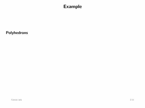
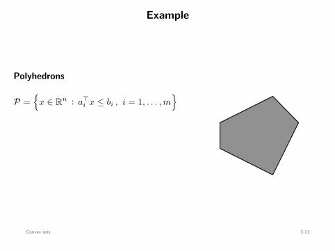
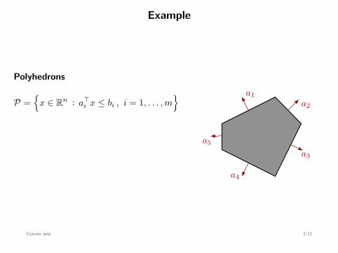
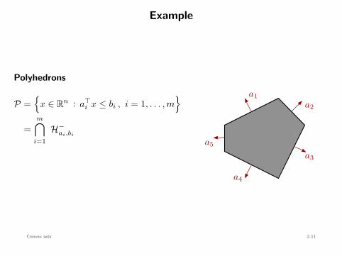
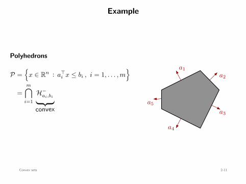
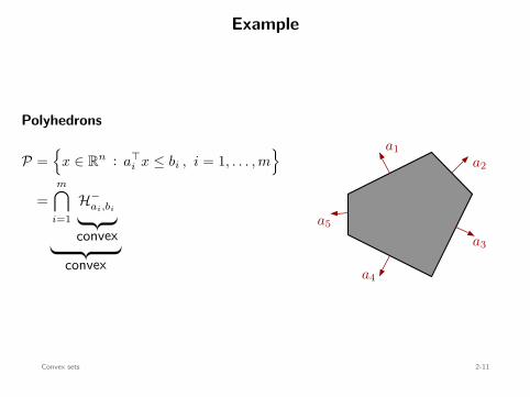
Example
Polyhedrons
P =
x ∈ Rn : a⊤i x ≤ bi , i = 1, . . . , m
=m∩
i=1H−
ai,bi
convex
convex
a1a2
a3
a4
a5
Convex sets 2-11
Example
Polyhedrons
P =
x ∈ Rn : a⊤i x ≤ bi , i = 1, . . . , m
=m∩
i=1H−
ai,bi
convex
convex
a1a2
a3
a4
a5
Convex sets 2-11
Example
Polyhedrons
P =
x ∈ Rn : a⊤i x ≤ bi , i = 1, . . . , m
=m∩
i=1H−
ai,bi
convex
convex
a1a2
a3
a4
a5
Convex sets 2-11
Example
Polyhedrons
P =
x ∈ Rn : a⊤i x ≤ bi , i = 1, . . . , m
=m∩
i=1H−
ai,bi
convex
convex
a1a2
a3
a4
a5
Convex sets 2-11
Example
Polyhedrons
P =
x ∈ Rn : a⊤i x ≤ bi , i = 1, . . . , m
=m∩
i=1H−
ai,bi
convex
convex
a1a2
a3
a4
a5
Convex sets 2-11
Example
Polyhedrons
P =
x ∈ Rn : a⊤i x ≤ bi , i = 1, . . . , m
=m∩
i=1H−
ai,bi
convex
convex
a1a2
a3
a4
a5
Convex sets 2-11
Example
Polyhedrons
P =
x ∈ Rn : a⊤i x ≤ bi , i = 1, . . . , m
=m∩
i=1H−
ai,bi
convex
convex
a1a2
a3
a4
a5
Convex sets 2-11
Example
Polyhedrons
P =
x ∈ Rn : a⊤i x ≤ bi , i = 1, . . . , m
=m∩
i=1H−
ai,bi
convex
convex
a1a2
a3
a4
a5
Convex sets 2-11

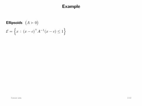
Example
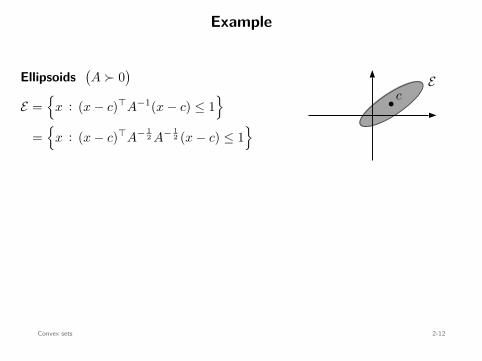
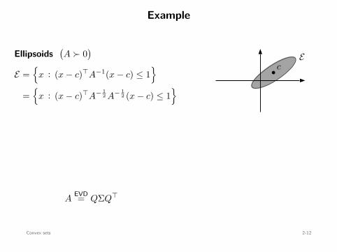
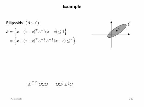
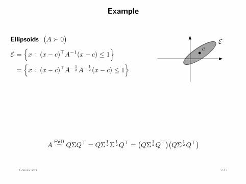
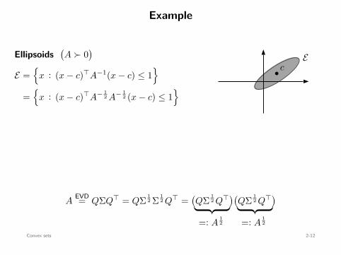
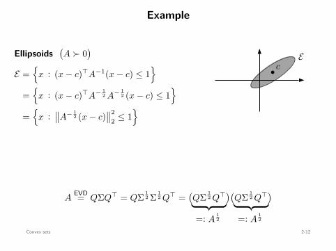
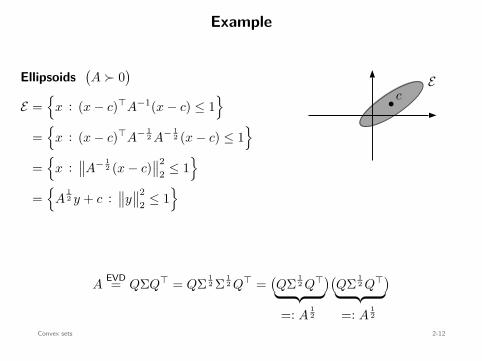
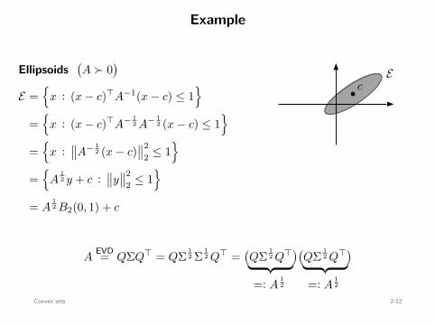
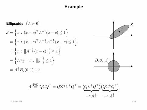
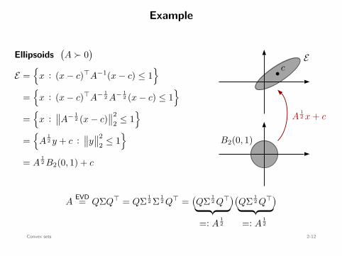
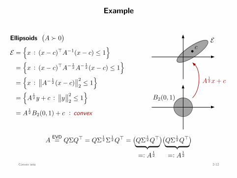
Ellipsoids
(A ≻ 0
)
E =
x : (x − c)⊤A−1(x − c) ≤ 1
=
x : (x − c)⊤A− 12 A− 1
2 (x − c) ≤ 1
=
x :∥∥A− 1
2 (x − c)∥∥2
2 ≤ 1
=
A12 y + c :
∥∥y∥∥2
2 ≤ 1
= A12 B2(0, 1) + c : convex
b cE
B2(0, 1)
A12 x + c
AEVD= QΣQ⊤ = QΣ 1
2 Σ 12 Q⊤ =
(QΣ 1
2 Q⊤)(QΣ 1
2 Q⊤)
=: A12 =: A
12
Convex sets 2-12
Example
Ellipsoids(A ≻ 0
)
E =
x : (x − c)⊤A−1(x − c) ≤ 1
=
x : (x − c)⊤A− 12 A− 1
2 (x − c) ≤ 1
=
x :∥∥A− 1
2 (x − c)∥∥2
2 ≤ 1
=
A12 y + c :
∥∥y∥∥2
2 ≤ 1
= A12 B2(0, 1) + c : convex
b cE
B2(0, 1)
A12 x + c
AEVD= QΣQ⊤ = QΣ 1
2 Σ 12 Q⊤ =
(QΣ 1
2 Q⊤)(QΣ 1
2 Q⊤)
=: A12 =: A
12
Convex sets 2-12
Example
Ellipsoids(A ≻ 0
)
E =
x : (x − c)⊤A−1(x − c) ≤ 1
=
x : (x − c)⊤A− 12 A− 1
2 (x − c) ≤ 1
=
x :∥∥A− 1
2 (x − c)∥∥2
2 ≤ 1
=
A12 y + c :
∥∥y∥∥2
2 ≤ 1
= A12 B2(0, 1) + c : convex
b cE
B2(0, 1)
A12 x + c
AEVD= QΣQ⊤ = QΣ 1
2 Σ 12 Q⊤ =
(QΣ 1
2 Q⊤)(QΣ 1
2 Q⊤)
=: A12 =: A
12
Convex sets 2-12
Example
Ellipsoids(A ≻ 0
)
E =
x : (x − c)⊤A−1(x − c) ≤ 1
=
x : (x − c)⊤A− 12 A− 1
2 (x − c) ≤ 1
=
x :∥∥A− 1
2 (x − c)∥∥2
2 ≤ 1
=
A12 y + c :
∥∥y∥∥2
2 ≤ 1
= A12 B2(0, 1) + c : convex
b cE
B2(0, 1)
A12 x + c
AEVD= QΣQ⊤ = QΣ 1
2 Σ 12 Q⊤ =
(QΣ 1
2 Q⊤)(QΣ 1
2 Q⊤)
=: A12 =: A
12
Convex sets 2-12
Example
Ellipsoids(A ≻ 0
)
E =
x : (x − c)⊤A−1(x − c) ≤ 1
=
x : (x − c)⊤A− 12 A− 1
2 (x − c) ≤ 1
=
x :∥∥A− 1
2 (x − c)∥∥2
2 ≤ 1
=
A12 y + c :
∥∥y∥∥2
2 ≤ 1
= A12 B2(0, 1) + c : convex
b cE
B2(0, 1)
A12 x + c
AEVD= QΣQ⊤
= QΣ 12 Σ 1
2 Q⊤ =(QΣ 1
2 Q⊤)(QΣ 1
2 Q⊤)
=: A12 =: A
12
Convex sets 2-12
Example
Ellipsoids(A ≻ 0
)
E =
x : (x − c)⊤A−1(x − c) ≤ 1
=
x : (x − c)⊤A− 12 A− 1
2 (x − c) ≤ 1
=
x :∥∥A− 1
2 (x − c)∥∥2
2 ≤ 1
=
A12 y + c :
∥∥y∥∥2
2 ≤ 1
= A12 B2(0, 1) + c : convex
b cE
B2(0, 1)
A12 x + c
AEVD= QΣQ⊤ = QΣ 1
2 Σ 12 Q⊤
=(QΣ 1
2 Q⊤)(QΣ 1
2 Q⊤)
=: A12 =: A
12
Convex sets 2-12
Example
Ellipsoids(A ≻ 0
)
E =
x : (x − c)⊤A−1(x − c) ≤ 1
=
x : (x − c)⊤A− 12 A− 1
2 (x − c) ≤ 1
=
x :∥∥A− 1
2 (x − c)∥∥2
2 ≤ 1
=
A12 y + c :
∥∥y∥∥2
2 ≤ 1
= A12 B2(0, 1) + c : convex
b cE
B2(0, 1)
A12 x + c
AEVD= QΣQ⊤ = QΣ 1
2 Σ 12 Q⊤ =
(QΣ 1
2 Q⊤)(QΣ 1
2 Q⊤)
=: A12 =: A
12
Convex sets 2-12
Example
Ellipsoids(A ≻ 0
)
E =
x : (x − c)⊤A−1(x − c) ≤ 1
=
x : (x − c)⊤A− 12 A− 1
2 (x − c) ≤ 1
=
x :∥∥A− 1
2 (x − c)∥∥2
2 ≤ 1
=
A12 y + c :
∥∥y∥∥2
2 ≤ 1
= A12 B2(0, 1) + c : convex
b cE
B2(0, 1)
A12 x + c
AEVD= QΣQ⊤ = QΣ 1
2 Σ 12 Q⊤ =
(QΣ 1
2 Q⊤)(QΣ 1
2 Q⊤)
=: A12 =: A
12
Convex sets 2-12
Example
Ellipsoids(A ≻ 0
)
E =
x : (x − c)⊤A−1(x − c) ≤ 1
=
x : (x − c)⊤A− 12 A− 1
2 (x − c) ≤ 1
=
x :∥∥A− 1
2 (x − c)∥∥2
2 ≤ 1
=
A12 y + c :
∥∥y∥∥2
2 ≤ 1
= A12 B2(0, 1) + c : convex
b cE
B2(0, 1)
A12 x + c
AEVD= QΣQ⊤ = QΣ 1
2 Σ 12 Q⊤ =
(QΣ 1
2 Q⊤)(QΣ 1
2 Q⊤)
=: A12 =: A
12
Convex sets 2-12
Example
Ellipsoids(A ≻ 0
)
E =
x : (x − c)⊤A−1(x − c) ≤ 1
=
x : (x − c)⊤A− 12 A− 1
2 (x − c) ≤ 1
=
x :∥∥A− 1
2 (x − c)∥∥2
2 ≤ 1
=
A12 y + c :
∥∥y∥∥2
2 ≤ 1
= A12 B2(0, 1) + c : convex
b cE
B2(0, 1)
A12 x + c
AEVD= QΣQ⊤ = QΣ 1
2 Σ 12 Q⊤ =
(QΣ 1
2 Q⊤)(QΣ 1
2 Q⊤)
=: A12 =: A
12
Convex sets 2-12
Example
Ellipsoids(A ≻ 0
)
E =
x : (x − c)⊤A−1(x − c) ≤ 1
=
x : (x − c)⊤A− 12 A− 1
2 (x − c) ≤ 1
=
x :∥∥A− 1
2 (x − c)∥∥2
2 ≤ 1
=
A12 y + c :
∥∥y∥∥2
2 ≤ 1
= A12 B2(0, 1) + c
: convex
b cE
B2(0, 1)
A12 x + c
AEVD= QΣQ⊤ = QΣ 1
2 Σ 12 Q⊤ =
(QΣ 1
2 Q⊤)(QΣ 1
2 Q⊤)
=: A12 =: A
12
Convex sets 2-12
Example
Ellipsoids(A ≻ 0
)
E =
x : (x − c)⊤A−1(x − c) ≤ 1
=
x : (x − c)⊤A− 12 A− 1
2 (x − c) ≤ 1
=
x :∥∥A− 1
2 (x − c)∥∥2
2 ≤ 1
=
A12 y + c :
∥∥y∥∥2
2 ≤ 1
= A12 B2(0, 1) + c
: convex
b cE
B2(0, 1)
A12 x + c
AEVD= QΣQ⊤ = QΣ 1
2 Σ 12 Q⊤ =
(QΣ 1
2 Q⊤)(QΣ 1
2 Q⊤)
=: A12 =: A
12
Convex sets 2-12
Example
Ellipsoids(A ≻ 0
)
E =
x : (x − c)⊤A−1(x − c) ≤ 1
=
x : (x − c)⊤A− 12 A− 1
2 (x − c) ≤ 1
=
x :∥∥A− 1
2 (x − c)∥∥2
2 ≤ 1
=
A12 y + c :
∥∥y∥∥2
2 ≤ 1
= A12 B2(0, 1) + c
: convex
b cE
B2(0, 1)
A12 x + c
AEVD= QΣQ⊤ = QΣ 1
2 Σ 12 Q⊤ =
(QΣ 1
2 Q⊤)(QΣ 1
2 Q⊤)
=: A12 =: A
12
Convex sets 2-12
Example
Ellipsoids(A ≻ 0
)
E =
x : (x − c)⊤A−1(x − c) ≤ 1
=
x : (x − c)⊤A− 12 A− 1
2 (x − c) ≤ 1
=
x :∥∥A− 1
2 (x − c)∥∥2
2 ≤ 1
=
A12 y + c :
∥∥y∥∥2
2 ≤ 1
= A12 B2(0, 1) + c : convex
b cE
B2(0, 1)
A12 x + c
AEVD= QΣQ⊤ = QΣ 1
2 Σ 12 Q⊤ =
(QΣ 1
2 Q⊤)(QΣ 1
2 Q⊤)
=: A12 =: A
12
Convex sets 2-12

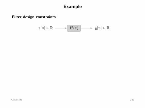
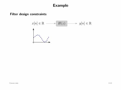
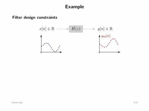
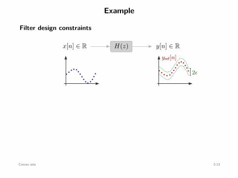
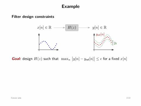
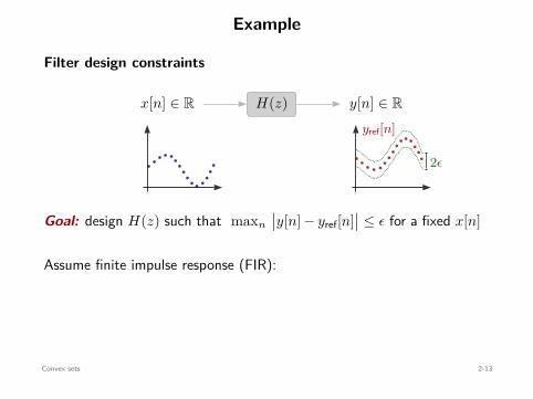
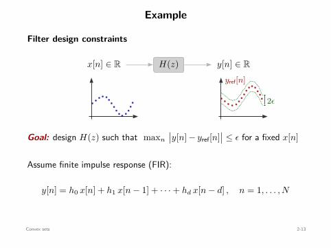
Example
Filter design constraints
x[n] ∈ R y[n] ∈ RH(z)yref[n]
2ϵ
Goal: design H(z) such that maxn
∣∣y[n] − yref[n]∣∣ ≤ ϵ for a fixed x[n]
Assume finite impulse response (FIR):
y[n] = h0 x[n] + h1 x[n − 1] + · · · + hd x[n − d] , n = 1, . . . , N
Convex sets 2-13
Example
Filter design constraints
x[n] ∈ R y[n] ∈ RH(z)yref[n]
2ϵ
Goal: design H(z) such that maxn
∣∣y[n] − yref[n]∣∣ ≤ ϵ for a fixed x[n]
Assume finite impulse response (FIR):
y[n] = h0 x[n] + h1 x[n − 1] + · · · + hd x[n − d] , n = 1, . . . , N
Convex sets 2-13
Example
Filter design constraints
x[n] ∈ R y[n] ∈ RH(z)
yref[n]
2ϵ
Goal: design H(z) such that maxn
∣∣y[n] − yref[n]∣∣ ≤ ϵ for a fixed x[n]
Assume finite impulse response (FIR):
y[n] = h0 x[n] + h1 x[n − 1] + · · · + hd x[n − d] , n = 1, . . . , N
Convex sets 2-13
Example
Filter design constraints
x[n] ∈ R y[n] ∈ RH(z)
yref[n]
2ϵ
Goal: design H(z) such that maxn
∣∣y[n] − yref[n]∣∣ ≤ ϵ for a fixed x[n]
Assume finite impulse response (FIR):
y[n] = h0 x[n] + h1 x[n − 1] + · · · + hd x[n − d] , n = 1, . . . , N
Convex sets 2-13
Example
Filter design constraints
x[n] ∈ R y[n] ∈ RH(z)yref[n]
2ϵ
Goal: design H(z) such that maxn
∣∣y[n] − yref[n]∣∣ ≤ ϵ for a fixed x[n]
Assume finite impulse response (FIR):
y[n] = h0 x[n] + h1 x[n − 1] + · · · + hd x[n − d] , n = 1, . . . , N
Convex sets 2-13
Example
Filter design constraints
x[n] ∈ R y[n] ∈ RH(z)yref[n]
2ϵ
Goal: design H(z) such that maxn
∣∣y[n] − yref[n]∣∣ ≤ ϵ for a fixed x[n]
Assume finite impulse response (FIR):
y[n] = h0 x[n] + h1 x[n − 1] + · · · + hd x[n − d] , n = 1, . . . , N
Convex sets 2-13
Example
Filter design constraints
x[n] ∈ R y[n] ∈ RH(z)yref[n]
2ϵ
Goal: design H(z) such that maxn
∣∣y[n] − yref[n]∣∣ ≤ ϵ for a fixed x[n]
Assume finite impulse response (FIR):
y[n] = h0 x[n] + h1 x[n − 1] + · · · + hd x[n − d] , n = 1, . . . , N
Convex sets 2-13
Example
Filter design constraints
x[n] ∈ R y[n] ∈ RH(z)yref[n]
2ϵ
Goal: design H(z) such that maxn
∣∣y[n] − yref[n]∣∣ ≤ ϵ for a fixed x[n]
Assume finite impulse response (FIR):
y[n] = h0 x[n] + h1 x[n − 1] + · · · + hd x[n − d] , n = 1, . . . , N
Convex sets 2-13
Example
Filter design constraints
x[n] ∈ R y[n] ∈ RH(z)yref[n]
2ϵ
Goal: design H(z) such that maxn
∣∣y[n] − yref[n]∣∣ ≤ ϵ for a fixed x[n]
Assume finite impulse response (FIR):
y[n] = h0 x[n] + h1 x[n − 1] + · · · + hd x[n − d] , n = 1, . . . , N
Convex sets 2-13
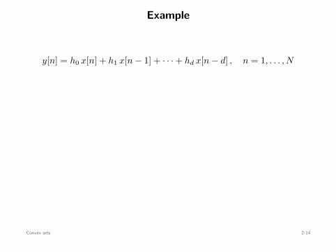
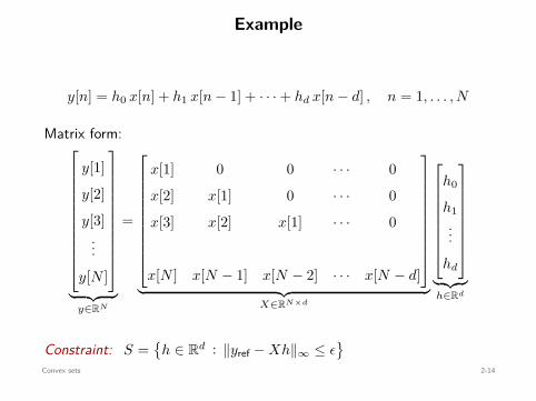
Example
y[n] = h0 x[n] + h1 x[n − 1] + · · · + hd x[n − d] , n = 1, . . . , N
Matrix form:
y[1]
y[2]
y[3]...
y[N ]
︸ ︷︷ ︸y∈RN
=
x[1] 0 0 · · · 0
x[2] x[1] 0 · · · 0
x[3] x[2] x[1] · · · 0
x[N ] x[N − 1] x[N − 2] · · · x[N − d]
︸ ︷︷ ︸X∈RN×d
h0
h1...
hd
︸ ︷︷ ︸h∈Rd
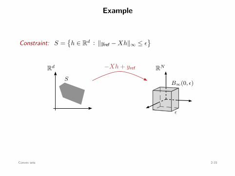
Constraint: S =
h ∈ Rd : ∥yref − Xh∥∞ ≤ ϵ
Convex sets 2-14

Example
y[n] = h0 x[n] + h1 x[n − 1] + · · · + hd x[n − d] , n = 1, . . . , N
Matrix form:
y[1]
y[2]
y[3]...
y[N ]
︸ ︷︷ ︸y∈RN
=
x[1] 0 0 · · · 0
x[2] x[1] 0 · · · 0
x[3] x[2] x[1] · · · 0
x[N ] x[N − 1] x[N − 2] · · · x[N − d]
︸ ︷︷ ︸X∈RN×d
h0
h1...
hd
︸ ︷︷ ︸h∈Rd
Constraint: S =
h ∈ Rd : ∥yref − Xh∥∞ ≤ ϵ
Convex sets 2-14
Example
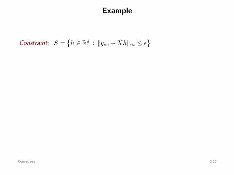
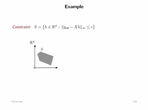
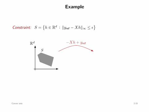
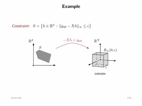
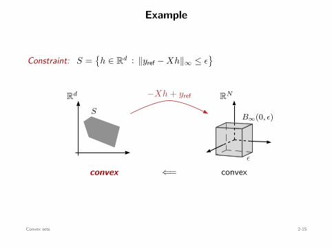
Constraint: S =
h ∈ Rd : ∥yref − Xh∥∞ ≤ ϵ
Rd
S
−Xh + yref RN
ϵ
B∞(0, ϵ)
convex⇐=convex
Convex sets 2-15
Example
Constraint: S =
h ∈ Rd : ∥yref − Xh∥∞ ≤ ϵ
Rd
S
−Xh + yref RN
ϵ
B∞(0, ϵ)
convex⇐=convex
Convex sets 2-15
Example
Constraint: S =
h ∈ Rd : ∥yref − Xh∥∞ ≤ ϵ
Rd
S
−Xh + yref
RN
ϵ
B∞(0, ϵ)
convex⇐=convex
Convex sets 2-15
Example
Constraint: S =
h ∈ Rd : ∥yref − Xh∥∞ ≤ ϵ
Rd
S
−Xh + yref RN
ϵ
B∞(0, ϵ)
convex⇐=convex
Convex sets 2-15
Example
Constraint: S =
h ∈ Rd : ∥yref − Xh∥∞ ≤ ϵ
Rd
S
−Xh + yref RN
ϵ
B∞(0, ϵ)
convex
⇐=convex
Convex sets 2-15
Example
Constraint: S =
h ∈ Rd : ∥yref − Xh∥∞ ≤ ϵ
Rd
S
−Xh + yref RN
ϵ
B∞(0, ϵ)
convex⇐=convex
Convex sets 2-15
Outline
Convex setsIdentifying convex setsExamples: geometrical sets and filter design constraints
Convex functionsIdentifying convex functionsRelation to convex sets
Optimization problemsConvex problems, properties, and problem manipulationExamples and solvers
Statistical estimationMaximum likelihood & maximum a posterioriNonparametric estimationHypothesis testing & optimal detection
Convex functions 2-1

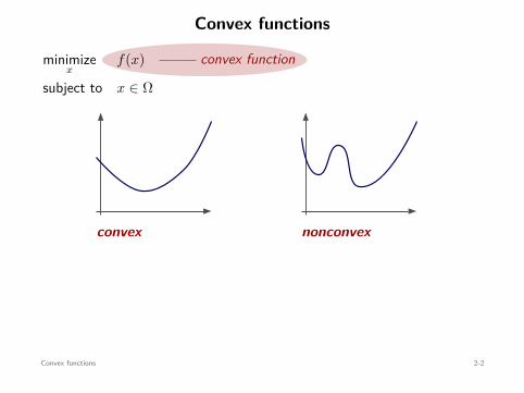
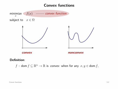
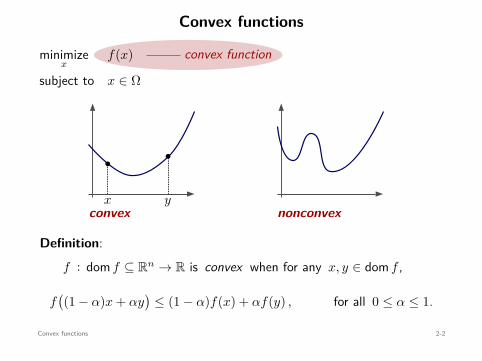
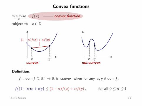
Convex functions
convex function
minimizex
f(x)
subject to x ∈ Ω
convex
bb
x y
(1 − α)f(x) + αf(y)
nonconvex
b
b
x y
Definition:f : dom f ⊆ Rn → R is convex when for any x, y ∈ dom f ,
f((1 − α)x + αy
)≤ (1 − α)f(x) + αf(y) , for all 0 ≤ α ≤ 1.
Convex functions 2-2
Convex functions
convex function
minimizex
f(x)
subject to x ∈ Ω
convex
bb
x y
(1 − α)f(x) + αf(y)
nonconvex
b
b
x y
Definition:f : dom f ⊆ Rn → R is convex when for any x, y ∈ dom f ,
f((1 − α)x + αy
)≤ (1 − α)f(x) + αf(y) , for all 0 ≤ α ≤ 1.
Convex functions 2-2
Convex functions
convex functionminimizex
f(x)
subject to x ∈ Ω
convex
bb
x y
(1 − α)f(x) + αf(y)
nonconvex
b
b
x y
Definition:f : dom f ⊆ Rn → R is convex when for any x, y ∈ dom f ,
f((1 − α)x + αy
)≤ (1 − α)f(x) + αf(y) , for all 0 ≤ α ≤ 1.
Convex functions 2-2
Convex functions
convex functionminimizex
f(x)
subject to x ∈ Ω
convex
bb
x y
(1 − α)f(x) + αf(y)
nonconvex
b
b
x y
Definition:f : dom f ⊆ Rn → R is convex when for any x, y ∈ dom f ,
f((1 − α)x + αy
)≤ (1 − α)f(x) + αf(y) , for all 0 ≤ α ≤ 1.
Convex functions 2-2
Convex functions
convex functionminimizex
f(x)
subject to x ∈ Ω
convex
bb
x y
(1 − α)f(x) + αf(y)
nonconvex
b
b
x y
Definition:f : dom f ⊆ Rn → R is convex when for any x, y ∈ dom f ,
f((1 − α)x + αy
)≤ (1 − α)f(x) + αf(y) , for all 0 ≤ α ≤ 1.
Convex functions 2-2
Convex functions
convex functionminimizex
f(x)
subject to x ∈ Ω
convex
bb
x y
(1 − α)f(x) + αf(y)
nonconvex
b
b
x y
Definition:f : dom f ⊆ Rn → R is convex when for any x, y ∈ dom f ,
f((1 − α)x + αy
)≤ (1 − α)f(x) + αf(y) , for all 0 ≤ α ≤ 1.
Convex functions 2-2

Convex functions
convex functionminimizex
f(x)
subject to x ∈ Ω
convex
bb
x y
(1 − α)f(x) + αf(y)
nonconvex
b
b
x y
Definition:f : dom f ⊆ Rn → R is convex when for any x, y ∈ dom f ,
f((1 − α)x + αy
)≤ (1 − α)f(x) + αf(y) , for all 0 ≤ α ≤ 1.
Convex functions 2-2
Convex functions
convex functionminimizex
f(x)
subject to x ∈ Ω
convex
bb
x y
(1 − α)f(x) + αf(y)
nonconvex
b
b
x y
Definition:f : dom f ⊆ Rn → R is convex when for any x, y ∈ dom f ,
f((1 − α)x + αy
)≤ (1 − α)f(x) + αf(y) , for all 0 ≤ α ≤ 1.
Convex functions 2-2

Convex functions
convex functionminimizex
f(x)
subject to x ∈ Ω
convex
bb
x y
(1 − α)f(x) + αf(y)
nonconvex
b
b
x y
Definition:f : dom f ⊆ Rn → R is convex when for any x, y ∈ dom f ,
f((1 − α)x + αy
)≤ (1 − α)f(x) + αf(y) , for all 0 ≤ α ≤ 1.
Convex functions 2-2

Convex functions
convex functionminimizex
f(x)
subject to x ∈ Ω
convex
bb
x y
(1 − α)f(x) + αf(y)
nonconvex
b
b
x y
Definition:f : dom f ⊆ Rn → R is convex when for any x, y ∈ dom f ,
f((1 − α)x + αy
)≤ (1 − α)f(x) + αf(y) , for all 0 ≤ α ≤ 1.
Convex functions 2-2
Convex functions
convex functionminimizex
f(x)
subject to x ∈ Ω
convex
bb
x y
(1 − α)f(x) + αf(y)
nonconvex
b
b
x y
Definition:f : dom f ⊆ Rn → R is convex when for any x, y ∈ dom f ,
f((1 − α)x + αy
)≤ (1 − α)f(x) + αf(y) , for all 0 ≤ α ≤ 1.
Convex functions 2-2

Convex functions
convex functionminimizex
f(x)
subject to x ∈ Ω
convex
bb
x y
(1 − α)f(x) + αf(y)
nonconvex
b
b
x y
Definition:f : dom f ⊆ Rn → R is convex when for any x, y ∈ dom f ,
f((1 − α)x + αy
)≤ (1 − α)f(x) + αf(y) , for all 0 ≤ α ≤ 1.
Convex functions 2-2
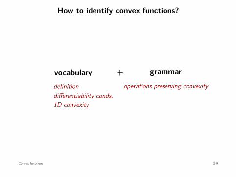
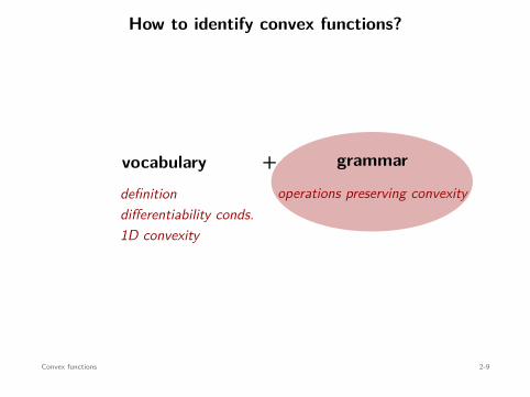
How to identify convex functions?
definitiondifferentiability conds.1D convexity
operations preserving convexity
vocabulary + grammar
Convex functions 2-3

How to identify convex functions?
definitiondifferentiability conds.1D convexity
operations preserving convexity
vocabulary + grammar
Convex functions 2-3

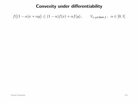
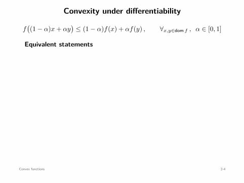
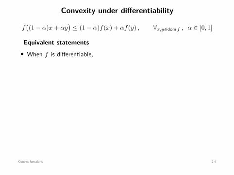
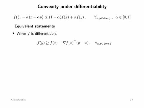
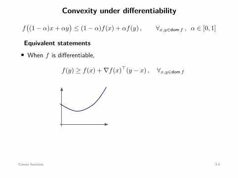
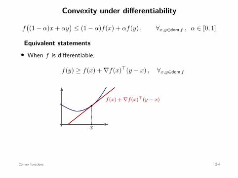
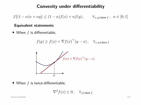
Convexity under differentiability
f((1 − α)x + αy
)≤ (1 − α)f(x) + αf(y) , ∀x,y∈dom f , α ∈ [0, 1]
Equivalent statements• When f is differentiable,
f(y) ≥ f(x) + ∇f(x)⊤(y − x) , ∀x,y∈dom f
f(x) + ∇f(x)⊤(y − x)b
x
• When f is twice-differentiable,
∇2f(x) ⪰ 0 , ∀x∈dom f
Convex functions 2-4
Convexity under differentiability
f((1 − α)x + αy
)≤ (1 − α)f(x) + αf(y) , ∀x,y∈dom f , α ∈ [0, 1]
Equivalent statements• When f is differentiable,
f(y) ≥ f(x) + ∇f(x)⊤(y − x) , ∀x,y∈dom f
f(x) + ∇f(x)⊤(y − x)b
x
• When f is twice-differentiable,
∇2f(x) ⪰ 0 , ∀x∈dom f
Convex functions 2-4
Convexity under differentiability
f((1 − α)x + αy
)≤ (1 − α)f(x) + αf(y) , ∀x,y∈dom f , α ∈ [0, 1]
Equivalent statements
• When f is differentiable,
f(y) ≥ f(x) + ∇f(x)⊤(y − x) , ∀x,y∈dom f
f(x) + ∇f(x)⊤(y − x)b
x
• When f is twice-differentiable,
∇2f(x) ⪰ 0 , ∀x∈dom f
Convex functions 2-4
Convexity under differentiability
f((1 − α)x + αy
)≤ (1 − α)f(x) + αf(y) , ∀x,y∈dom f , α ∈ [0, 1]
Equivalent statements• When f is differentiable,
f(y) ≥ f(x) + ∇f(x)⊤(y − x) , ∀x,y∈dom f
f(x) + ∇f(x)⊤(y − x)b
x
• When f is twice-differentiable,
∇2f(x) ⪰ 0 , ∀x∈dom f
Convex functions 2-4
Convexity under differentiability
f((1 − α)x + αy
)≤ (1 − α)f(x) + αf(y) , ∀x,y∈dom f , α ∈ [0, 1]
Equivalent statements• When f is differentiable,
f(y) ≥ f(x) + ∇f(x)⊤(y − x) , ∀x,y∈dom f
f(x) + ∇f(x)⊤(y − x)b
x
• When f is twice-differentiable,
∇2f(x) ⪰ 0 , ∀x∈dom f
Convex functions 2-4
Convexity under differentiability
f((1 − α)x + αy
)≤ (1 − α)f(x) + αf(y) , ∀x,y∈dom f , α ∈ [0, 1]
Equivalent statements• When f is differentiable,
f(y) ≥ f(x) + ∇f(x)⊤(y − x) , ∀x,y∈dom f
f(x) + ∇f(x)⊤(y − x)b
x
• When f is twice-differentiable,
∇2f(x) ⪰ 0 , ∀x∈dom f
Convex functions 2-4

Convexity under differentiability
f((1 − α)x + αy
)≤ (1 − α)f(x) + αf(y) , ∀x,y∈dom f , α ∈ [0, 1]
Equivalent statements• When f is differentiable,
f(y) ≥ f(x) + ∇f(x)⊤(y − x) , ∀x,y∈dom f
f(x) + ∇f(x)⊤(y − x)
b
x
• When f is twice-differentiable,
∇2f(x) ⪰ 0 , ∀x∈dom f
Convex functions 2-4
Convexity under differentiability
f((1 − α)x + αy
)≤ (1 − α)f(x) + αf(y) , ∀x,y∈dom f , α ∈ [0, 1]
Equivalent statements• When f is differentiable,
f(y) ≥ f(x) + ∇f(x)⊤(y − x) , ∀x,y∈dom f
f(x) + ∇f(x)⊤(y − x)b
x
• When f is twice-differentiable,
∇2f(x) ⪰ 0 , ∀x∈dom f
Convex functions 2-4
Convexity under differentiability
f((1 − α)x + αy
)≤ (1 − α)f(x) + αf(y) , ∀x,y∈dom f , α ∈ [0, 1]
Equivalent statements• When f is differentiable,
f(y) ≥ f(x) + ∇f(x)⊤(y − x) , ∀x,y∈dom f
f(x) + ∇f(x)⊤(y − x)b
x
• When f is twice-differentiable,
∇2f(x) ⪰ 0 , ∀x∈dom f
Convex functions 2-4

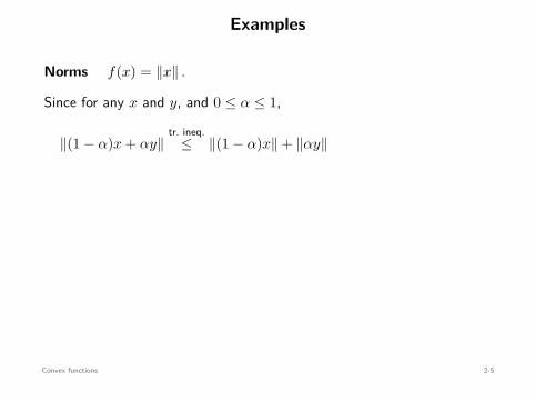
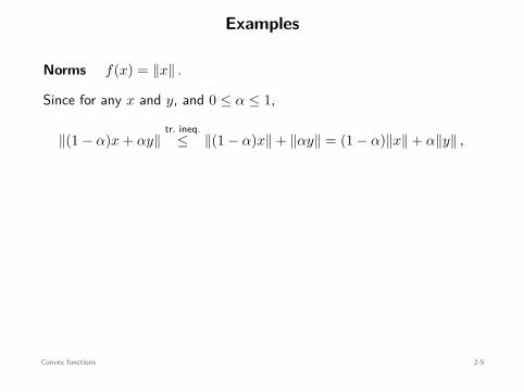
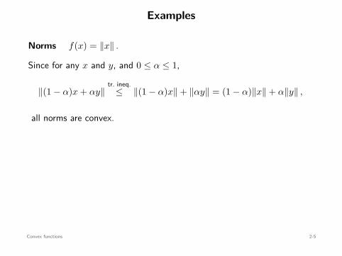
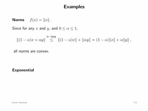
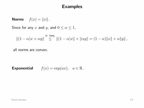
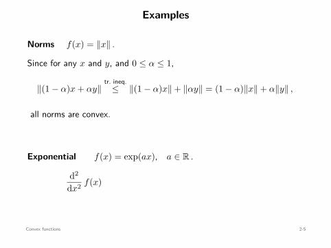
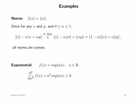
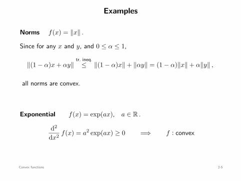
Examples
Norms f(x) = ∥x∥ .
Since for any x and y, and 0 ≤ α ≤ 1,
∥(1 − α)x + αy∥tr. ineq.
≤ ∥(1 − α)x∥ + ∥αy∥ = (1 − α)∥x∥ + α∥y∥ ,
all norms are convex.
Exponential f(x) = exp(ax), a ∈ R .
d2
dx2 f(x) = a2 exp(ax) ≥ 0 =⇒ f : convex
Convex functions 2-5
Examples
Norms f(x) = ∥x∥ .
Since for any x and y, and 0 ≤ α ≤ 1,
∥(1 − α)x + αy∥tr. ineq.
≤ ∥(1 − α)x∥ + ∥αy∥ = (1 − α)∥x∥ + α∥y∥ ,
all norms are convex.
Exponential f(x) = exp(ax), a ∈ R .
d2
dx2 f(x) = a2 exp(ax) ≥ 0 =⇒ f : convex
Convex functions 2-5

Examples
Norms f(x) = ∥x∥ .
Since for any x and y, and 0 ≤ α ≤ 1,
∥(1 − α)x + αy∥
tr. ineq.≤ ∥(1 − α)x∥ + ∥αy∥ = (1 − α)∥x∥ + α∥y∥ ,
all norms are convex.
Exponential f(x) = exp(ax), a ∈ R .
d2
dx2 f(x) = a2 exp(ax) ≥ 0 =⇒ f : convex
Convex functions 2-5
Examples
Norms f(x) = ∥x∥ .
Since for any x and y, and 0 ≤ α ≤ 1,
∥(1 − α)x + αy∥tr. ineq.
≤ ∥(1 − α)x∥ + ∥αy∥
= (1 − α)∥x∥ + α∥y∥ ,
all norms are convex.
Exponential f(x) = exp(ax), a ∈ R .
d2
dx2 f(x) = a2 exp(ax) ≥ 0 =⇒ f : convex
Convex functions 2-5
Examples
Norms f(x) = ∥x∥ .
Since for any x and y, and 0 ≤ α ≤ 1,
∥(1 − α)x + αy∥tr. ineq.
≤ ∥(1 − α)x∥ + ∥αy∥ = (1 − α)∥x∥ + α∥y∥ ,
all norms are convex.
Exponential f(x) = exp(ax), a ∈ R .
d2
dx2 f(x) = a2 exp(ax) ≥ 0 =⇒ f : convex
Convex functions 2-5
Examples
Norms f(x) = ∥x∥ .
Since for any x and y, and 0 ≤ α ≤ 1,
∥(1 − α)x + αy∥tr. ineq.
≤ ∥(1 − α)x∥ + ∥αy∥ = (1 − α)∥x∥ + α∥y∥ ,
all norms are convex.
Exponential f(x) = exp(ax), a ∈ R .
d2
dx2 f(x) = a2 exp(ax) ≥ 0 =⇒ f : convex
Convex functions 2-5
Examples
Norms f(x) = ∥x∥ .
Since for any x and y, and 0 ≤ α ≤ 1,
∥(1 − α)x + αy∥tr. ineq.
≤ ∥(1 − α)x∥ + ∥αy∥ = (1 − α)∥x∥ + α∥y∥ ,
all norms are convex.
Exponential
f(x) = exp(ax), a ∈ R .
d2
dx2 f(x) = a2 exp(ax) ≥ 0 =⇒ f : convex
Convex functions 2-5
Examples
Norms f(x) = ∥x∥ .
Since for any x and y, and 0 ≤ α ≤ 1,
∥(1 − α)x + αy∥tr. ineq.
≤ ∥(1 − α)x∥ + ∥αy∥ = (1 − α)∥x∥ + α∥y∥ ,
all norms are convex.
Exponential f(x) = exp(ax), a ∈ R .
d2
dx2 f(x) = a2 exp(ax) ≥ 0 =⇒ f : convex
Convex functions 2-5
Examples
Norms f(x) = ∥x∥ .
Since for any x and y, and 0 ≤ α ≤ 1,
∥(1 − α)x + αy∥tr. ineq.
≤ ∥(1 − α)x∥ + ∥αy∥ = (1 − α)∥x∥ + α∥y∥ ,
all norms are convex.
Exponential f(x) = exp(ax), a ∈ R .
d2
dx2 f(x)
= a2 exp(ax) ≥ 0 =⇒ f : convex
Convex functions 2-5
Examples
Norms f(x) = ∥x∥ .
Since for any x and y, and 0 ≤ α ≤ 1,
∥(1 − α)x + αy∥tr. ineq.
≤ ∥(1 − α)x∥ + ∥αy∥ = (1 − α)∥x∥ + α∥y∥ ,
all norms are convex.
Exponential f(x) = exp(ax), a ∈ R .
d2
dx2 f(x) = a2 exp(ax) ≥ 0
=⇒ f : convex
Convex functions 2-5
Examples
Norms f(x) = ∥x∥ .
Since for any x and y, and 0 ≤ α ≤ 1,
∥(1 − α)x + αy∥tr. ineq.
≤ ∥(1 − α)x∥ + ∥αy∥ = (1 − α)∥x∥ + α∥y∥ ,
all norms are convex.
Exponential f(x) = exp(ax), a ∈ R .
d2
dx2 f(x) = a2 exp(ax) ≥ 0 =⇒ f : convex
Convex functions 2-5
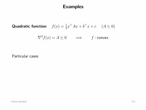
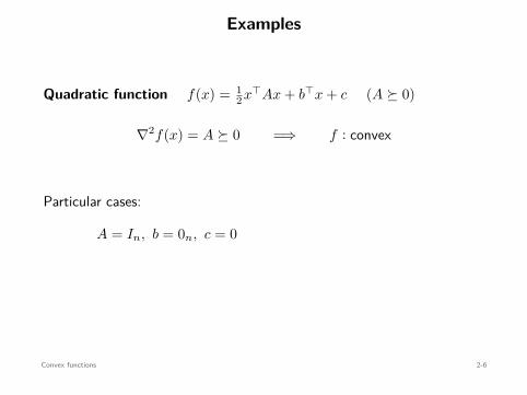
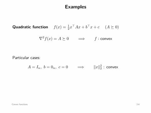
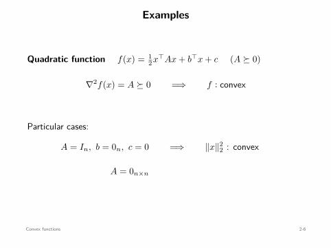
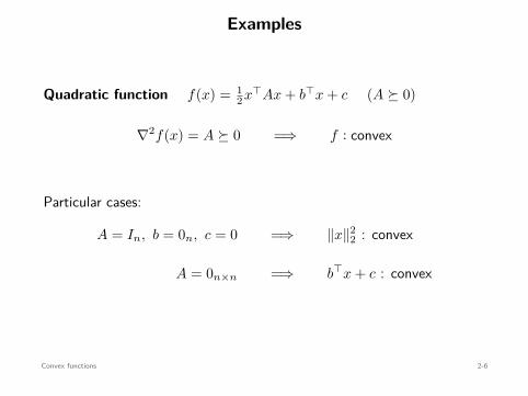
Examples
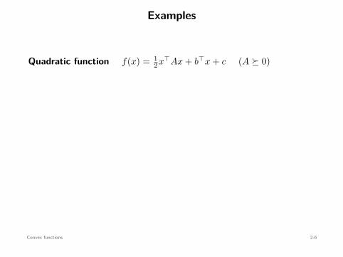
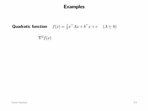
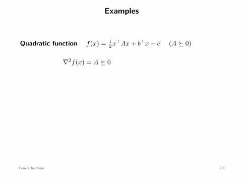
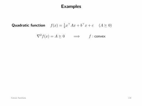
Quadratic function f(x) = 12 x⊤Ax + b⊤x + c (A ⪰ 0)
∇2f(x) = A ⪰ 0 =⇒ f : convex
Particular cases:
A = In, b = 0n, c = 0 =⇒ ∥x∥22 : convex
A = 0n×n =⇒ b⊤x + c : convex
Convex functions 2-6
Examples
Quadratic function f(x) = 12 x⊤Ax + b⊤x + c (A ⪰ 0)
∇2f(x)
= A ⪰ 0 =⇒ f : convex
Particular cases:
A = In, b = 0n, c = 0 =⇒ ∥x∥22 : convex
A = 0n×n =⇒ b⊤x + c : convex
Convex functions 2-6
Examples
Quadratic function f(x) = 12 x⊤Ax + b⊤x + c (A ⪰ 0)
∇2f(x) = A ⪰ 0
=⇒ f : convex
Particular cases:
A = In, b = 0n, c = 0 =⇒ ∥x∥22 : convex
A = 0n×n =⇒ b⊤x + c : convex
Convex functions 2-6
Examples
Quadratic function f(x) = 12 x⊤Ax + b⊤x + c (A ⪰ 0)
∇2f(x) = A ⪰ 0 =⇒ f : convex
Particular cases:
A = In, b = 0n, c = 0 =⇒ ∥x∥22 : convex
A = 0n×n =⇒ b⊤x + c : convex
Convex functions 2-6
Examples
Quadratic function f(x) = 12 x⊤Ax + b⊤x + c (A ⪰ 0)
∇2f(x) = A ⪰ 0 =⇒ f : convex
Particular cases:
A = In, b = 0n, c = 0 =⇒ ∥x∥22 : convex
A = 0n×n =⇒ b⊤x + c : convex
Convex functions 2-6
Examples
Quadratic function f(x) = 12 x⊤Ax + b⊤x + c (A ⪰ 0)
∇2f(x) = A ⪰ 0 =⇒ f : convex
Particular cases:
A = In, b = 0n, c = 0
=⇒ ∥x∥22 : convex
A = 0n×n =⇒ b⊤x + c : convex
Convex functions 2-6
Examples
Quadratic function f(x) = 12 x⊤Ax + b⊤x + c (A ⪰ 0)
∇2f(x) = A ⪰ 0 =⇒ f : convex
Particular cases:
A = In, b = 0n, c = 0 =⇒ ∥x∥22 : convex
A = 0n×n =⇒ b⊤x + c : convex
Convex functions 2-6
Examples
Quadratic function f(x) = 12 x⊤Ax + b⊤x + c (A ⪰ 0)
∇2f(x) = A ⪰ 0 =⇒ f : convex
Particular cases:
A = In, b = 0n, c = 0 =⇒ ∥x∥22 : convex
A = 0n×n
=⇒ b⊤x + c : convex
Convex functions 2-6
Examples
Quadratic function f(x) = 12 x⊤Ax + b⊤x + c (A ⪰ 0)
∇2f(x) = A ⪰ 0 =⇒ f : convex
Particular cases:
A = In, b = 0n, c = 0 =⇒ ∥x∥22 : convex
A = 0n×n =⇒ b⊤x + c : convex
Convex functions 2-6
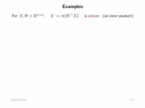
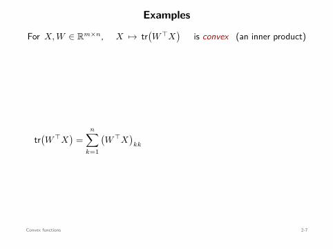
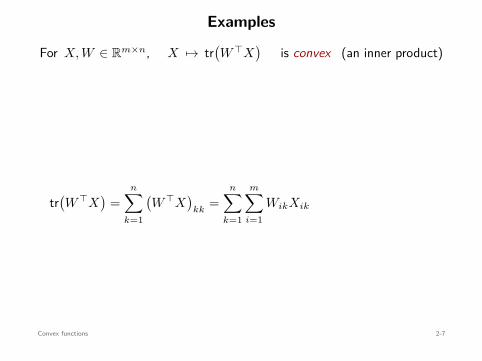
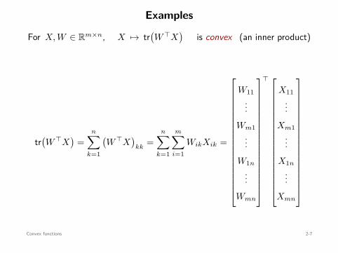
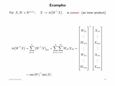
Examples
For X, W ∈ Rm×n, X 7→ tr(W ⊤X
)
is convex (an inner product)
tr(W ⊤X
)=
n∑
k=1
(W ⊤X
)kk
=n∑
k=1
m∑
i=1WikXik =
W11...
Wm1...
W1n
...Wmn
⊤
X11...
Xm1...
X1n
...Xmn
= vec(W )⊤vec(X)
Convex functions 2-7
Examples
For X, W ∈ Rm×n, X 7→ tr(W ⊤X
)is convex (an inner product)
tr(W ⊤X
)=
n∑
k=1
(W ⊤X
)kk
=n∑
k=1
m∑
i=1WikXik =
W11...
Wm1...
W1n
...Wmn
⊤
X11...
Xm1...
X1n
...Xmn
= vec(W )⊤vec(X)
Convex functions 2-7
Examples
For X, W ∈ Rm×n, X 7→ tr(W ⊤X
)is convex (an inner product)
tr(W ⊤X
)=
n∑
k=1
(W ⊤X
)kk
=n∑
k=1
m∑
i=1WikXik =
W11...
Wm1...
W1n
...Wmn
⊤
X11...
Xm1...
X1n
...Xmn
= vec(W )⊤vec(X)
Convex functions 2-7
Examples
For X, W ∈ Rm×n, X 7→ tr(W ⊤X
)is convex (an inner product)
tr(W ⊤X
)=
n∑
k=1
(W ⊤X
)kk
=n∑
k=1
m∑
i=1WikXik
=
W11...
Wm1...
W1n
...Wmn
⊤
X11...
Xm1...
X1n
...Xmn
= vec(W )⊤vec(X)
Convex functions 2-7
Examples
For X, W ∈ Rm×n, X 7→ tr(W ⊤X
)is convex (an inner product)
tr(W ⊤X
)=
n∑
k=1
(W ⊤X
)kk
=n∑
k=1
m∑
i=1WikXik =
W11...
Wm1...
W1n
...Wmn
⊤
X11...
Xm1...
X1n
...Xmn
= vec(W )⊤vec(X)
Convex functions 2-7
Examples
For X, W ∈ Rm×n, X 7→ tr(W ⊤X
)is convex (an inner product)
tr(W ⊤X
)=
n∑
k=1
(W ⊤X
)kk
=n∑
k=1
m∑
i=1WikXik =
W11...
Wm1...
W1n
...Wmn
⊤
X11...
Xm1...
X1n
...Xmn
= vec(W )⊤vec(X)Convex functions 2-7
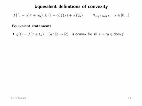
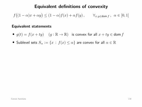
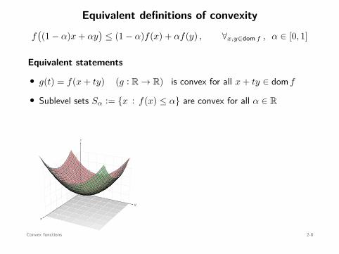
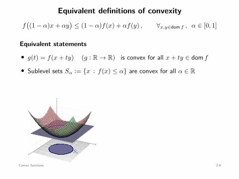
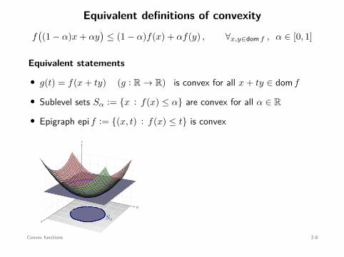
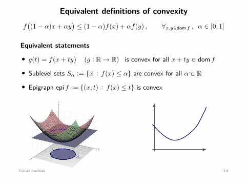
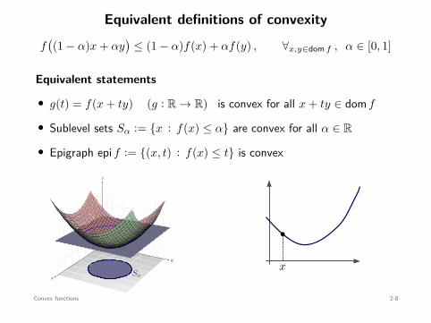
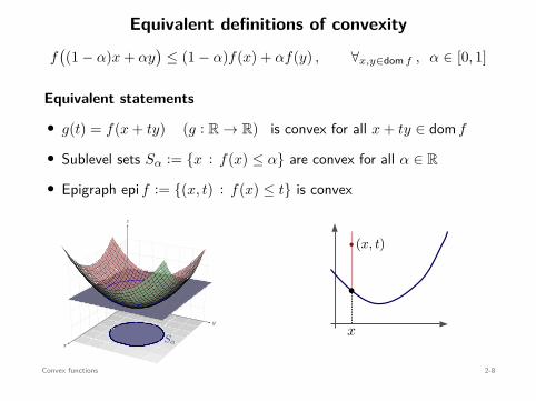
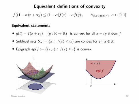
Equivalent definitions of convexity
f((1 − α)x + αy
)≤ (1 − α)f(x) + αf(y) , ∀x,y∈dom f , α ∈ [0, 1]
Equivalent statements
• g(t) = f(x + ty) (g : R → R) is convex for all x + ty ∈ dom f
• Sublevel sets Sα := x : f(x) ≤ α are convex for all α ∈ R
• Epigraph epi f := (x, t) : f(x) ≤ t is convex
x
y
z
Sα
b
x
b (x, t)
epi f
Convex functions 2-8
How to identify convex functions?
definitiondifferentiability conds.1D convexity
operations preserving convexity
vocabulary + grammar
Convex functions 2-9
How to identify convex functions?
definitiondifferentiability conds.1D convexity
operations preserving convexity
vocabulary + grammar
Convex functions 2-9

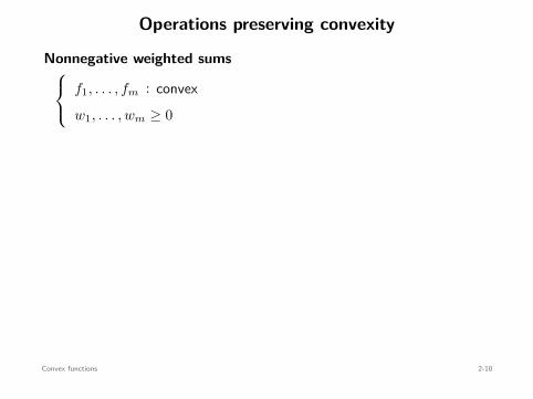
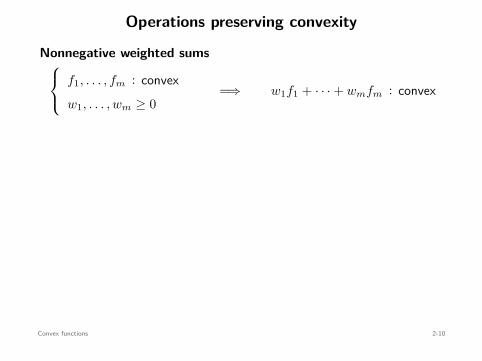
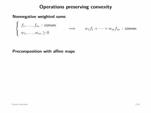
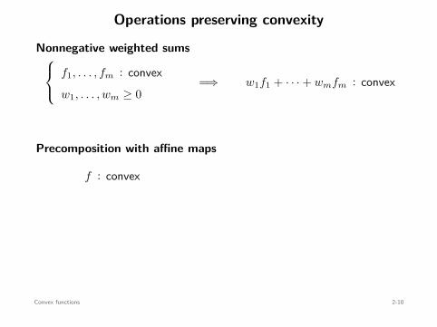
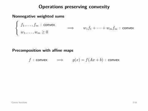
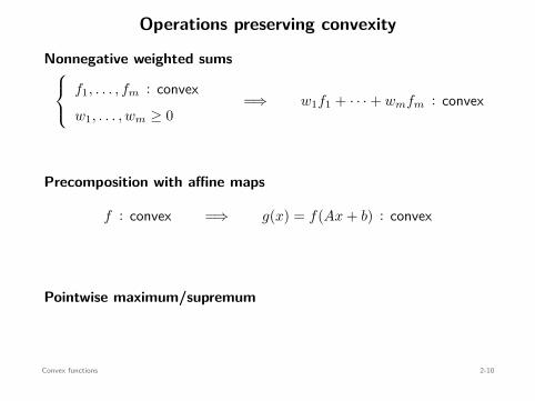
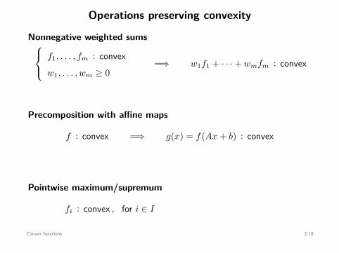
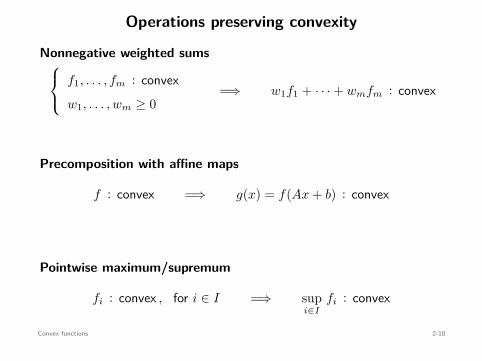
Operations preserving convexity
Nonnegative weighted sums
f1, . . . , fm : convexw1, . . . , wm ≥ 0
=⇒ w1f1 + · · · + wmfm : convex
Precomposition with affine maps
f : convex =⇒ g(x) = f(Ax + b) : convex
Pointwise maximum/supremum
fi : convex , for i ∈ I =⇒ supi∈I
fi : convex
Convex functions 2-10
Operations preserving convexity
Nonnegative weighted sums
f1, . . . , fm : convexw1, . . . , wm ≥ 0
=⇒ w1f1 + · · · + wmfm : convex
Precomposition with affine maps
f : convex =⇒ g(x) = f(Ax + b) : convex
Pointwise maximum/supremum
fi : convex , for i ∈ I =⇒ supi∈I
fi : convex
Convex functions 2-10
Operations preserving convexity
Nonnegative weighted sums
f1, . . . , fm : convexw1, . . . , wm ≥ 0
=⇒ w1f1 + · · · + wmfm : convex
Precomposition with affine maps
f : convex =⇒ g(x) = f(Ax + b) : convex
Pointwise maximum/supremum
fi : convex , for i ∈ I =⇒ supi∈I
fi : convex
Convex functions 2-10
Operations preserving convexity
Nonnegative weighted sums
f1, . . . , fm : convexw1, . . . , wm ≥ 0
=⇒ w1f1 + · · · + wmfm : convex
Precomposition with affine maps
f : convex =⇒ g(x) = f(Ax + b) : convex
Pointwise maximum/supremum
fi : convex , for i ∈ I =⇒ supi∈I
fi : convex
Convex functions 2-10
Operations preserving convexity
Nonnegative weighted sums
f1, . . . , fm : convexw1, . . . , wm ≥ 0
=⇒ w1f1 + · · · + wmfm : convex
Precomposition with affine maps
f : convex =⇒ g(x) = f(Ax + b) : convex
Pointwise maximum/supremum
fi : convex , for i ∈ I =⇒ supi∈I
fi : convex
Convex functions 2-10
Operations preserving convexity
Nonnegative weighted sums
f1, . . . , fm : convexw1, . . . , wm ≥ 0
=⇒ w1f1 + · · · + wmfm : convex
Precomposition with affine maps
f : convex
=⇒ g(x) = f(Ax + b) : convex
Pointwise maximum/supremum
fi : convex , for i ∈ I =⇒ supi∈I
fi : convex
Convex functions 2-10
Operations preserving convexity
Nonnegative weighted sums
f1, . . . , fm : convexw1, . . . , wm ≥ 0
=⇒ w1f1 + · · · + wmfm : convex
Precomposition with affine maps
f : convex =⇒ g(x) = f(Ax + b) : convex
Pointwise maximum/supremum
fi : convex , for i ∈ I =⇒ supi∈I
fi : convex
Convex functions 2-10
Operations preserving convexity
Nonnegative weighted sums
f1, . . . , fm : convexw1, . . . , wm ≥ 0
=⇒ w1f1 + · · · + wmfm : convex
Precomposition with affine maps
f : convex =⇒ g(x) = f(Ax + b) : convex
Pointwise maximum/supremum
fi : convex , for i ∈ I =⇒ supi∈I
fi : convex
Convex functions 2-10
Operations preserving convexity
Nonnegative weighted sums
f1, . . . , fm : convexw1, . . . , wm ≥ 0
=⇒ w1f1 + · · · + wmfm : convex
Precomposition with affine maps
f : convex =⇒ g(x) = f(Ax + b) : convex
Pointwise maximum/supremum
fi : convex , for i ∈ I
=⇒ supi∈I
fi : convex
Convex functions 2-10
Operations preserving convexity
Nonnegative weighted sums
f1, . . . , fm : convexw1, . . . , wm ≥ 0
=⇒ w1f1 + · · · + wmfm : convex
Precomposition with affine maps
f : convex =⇒ g(x) = f(Ax + b) : convex
Pointwise maximum/supremum
fi : convex , for i ∈ I =⇒ supi∈I
fi : convex
Convex functions 2-10
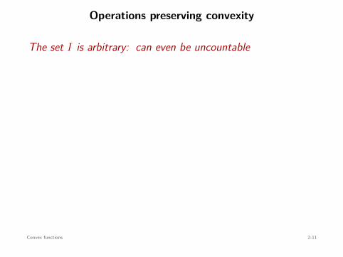
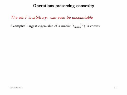
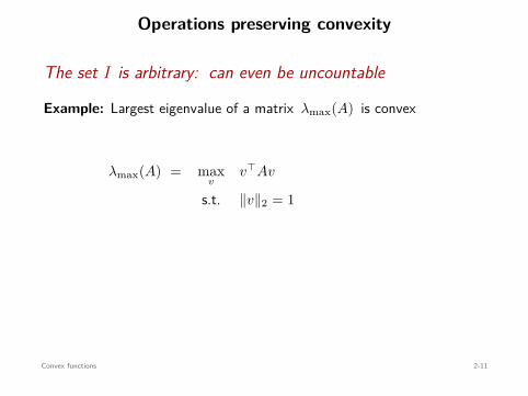
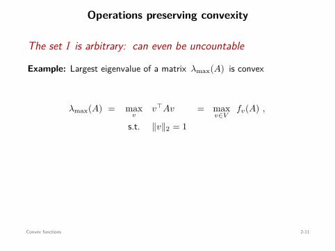
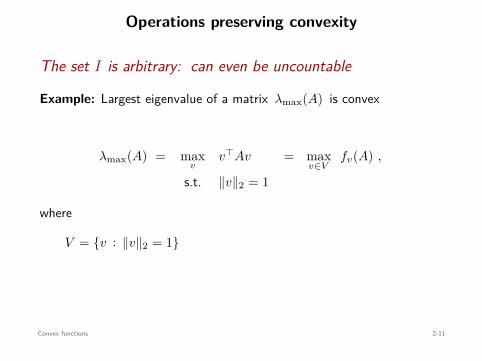
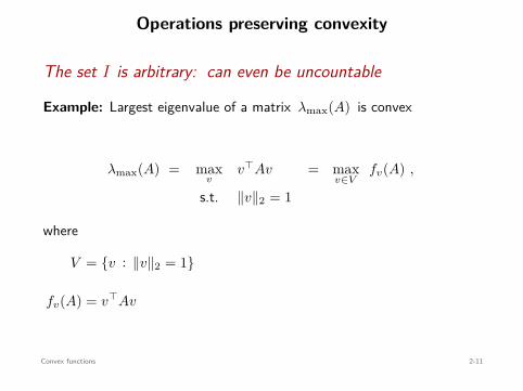
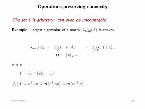
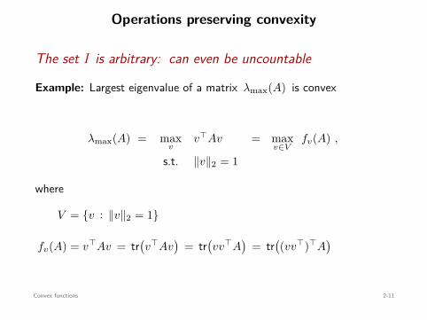
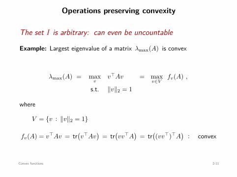
Operations preserving convexity
The set I is arbitrary: can even be uncountable
Example: Largest eigenvalue of a matrix λmax(A) is convex
λmax(A) = maxv
v⊤Av
s.t. ∥v∥2 = 1
= maxv∈V
fv(A) ,
where
V = v : ∥v∥2 = 1
fv(A) = v⊤Av = tr(v⊤Av
)= tr
(vv⊤A
)= tr
((vv⊤)⊤A
): convex
Convex functions 2-11
Operations preserving convexity
The set I is arbitrary: can even be uncountable
Example: Largest eigenvalue of a matrix λmax(A) is convex
λmax(A) = maxv
v⊤Av
s.t. ∥v∥2 = 1
= maxv∈V
fv(A) ,
where
V = v : ∥v∥2 = 1
fv(A) = v⊤Av = tr(v⊤Av
)= tr
(vv⊤A
)= tr
((vv⊤)⊤A
): convex
Convex functions 2-11
Operations preserving convexity
The set I is arbitrary: can even be uncountable
Example: Largest eigenvalue of a matrix λmax(A) is convex
λmax(A) = maxv
v⊤Av
s.t. ∥v∥2 = 1
= maxv∈V
fv(A) ,
where
V = v : ∥v∥2 = 1
fv(A) = v⊤Av = tr(v⊤Av
)= tr
(vv⊤A
)= tr
((vv⊤)⊤A
): convex
Convex functions 2-11
Operations preserving convexity
The set I is arbitrary: can even be uncountable
Example: Largest eigenvalue of a matrix λmax(A) is convex
λmax(A) = maxv
v⊤Av
s.t. ∥v∥2 = 1
= maxv∈V
fv(A) ,
where
V = v : ∥v∥2 = 1
fv(A) = v⊤Av = tr(v⊤Av
)= tr
(vv⊤A
)= tr
((vv⊤)⊤A
): convex
Convex functions 2-11
Operations preserving convexity
The set I is arbitrary: can even be uncountable
Example: Largest eigenvalue of a matrix λmax(A) is convex
λmax(A) = maxv
v⊤Av
s.t. ∥v∥2 = 1
= maxv∈V
fv(A) ,
where
V = v : ∥v∥2 = 1
fv(A) = v⊤Av = tr(v⊤Av
)= tr
(vv⊤A
)= tr
((vv⊤)⊤A
): convex
Convex functions 2-11
Operations preserving convexity
The set I is arbitrary: can even be uncountable
Example: Largest eigenvalue of a matrix λmax(A) is convex
λmax(A) = maxv
v⊤Av
s.t. ∥v∥2 = 1
= maxv∈V
fv(A) ,
where
V = v : ∥v∥2 = 1
fv(A) = v⊤Av
= tr(v⊤Av
)= tr
(vv⊤A
)= tr
((vv⊤)⊤A
): convex
Convex functions 2-11
Operations preserving convexity
The set I is arbitrary: can even be uncountable
Example: Largest eigenvalue of a matrix λmax(A) is convex
λmax(A) = maxv
v⊤Av
s.t. ∥v∥2 = 1
= maxv∈V
fv(A) ,
where
V = v : ∥v∥2 = 1
fv(A) = v⊤Av = tr(v⊤Av
)
= tr(vv⊤A
)= tr
((vv⊤)⊤A
): convex
Convex functions 2-11
Operations preserving convexity
The set I is arbitrary: can even be uncountable
Example: Largest eigenvalue of a matrix λmax(A) is convex
λmax(A) = maxv
v⊤Av
s.t. ∥v∥2 = 1
= maxv∈V
fv(A) ,
where
V = v : ∥v∥2 = 1
fv(A) = v⊤Av = tr(v⊤Av
)= tr
(vv⊤A
)
= tr((vv⊤)⊤A
): convex
Convex functions 2-11
Operations preserving convexity
The set I is arbitrary: can even be uncountable
Example: Largest eigenvalue of a matrix λmax(A) is convex
λmax(A) = maxv
v⊤Av
s.t. ∥v∥2 = 1
= maxv∈V
fv(A) ,
where
V = v : ∥v∥2 = 1
fv(A) = v⊤Av = tr(v⊤Av
)= tr
(vv⊤A
)= tr
((vv⊤)⊤A
)
: convex
Convex functions 2-11
Operations preserving convexity
The set I is arbitrary: can even be uncountable
Example: Largest eigenvalue of a matrix λmax(A) is convex
λmax(A) = maxv
v⊤Av
s.t. ∥v∥2 = 1
= maxv∈V
fv(A) ,
where
V = v : ∥v∥2 = 1
fv(A) = v⊤Av = tr(v⊤Av
)= tr
(vv⊤A
)= tr
((vv⊤)⊤A
): convex
Convex functions 2-11

Examples
• f(x) =∥∥y − Ax
∥∥22 = g(h(x)) : convex
h(x) = −Ax + y affine
g(z) = ∥z∥22 convex
• f(x) =∥∥y − Ax
∥∥1 = g(h(x)) : convex
h(x) = −Ax + y affine
g(z) = ∥z∥1 convex
Convex functions 2-12
Examples
• f(x) =∥∥y − Ax
∥∥22
= g(h(x)) : convex
h(x) = −Ax + y affine
g(z) = ∥z∥22 convex
• f(x) =∥∥y − Ax
∥∥1 = g(h(x)) : convex
h(x) = −Ax + y affine
g(z) = ∥z∥1 convex
Convex functions 2-12
Examples
• f(x) =∥∥y − Ax
∥∥22 = g(h(x))
: convex
h(x) = −Ax + y affine
g(z) = ∥z∥22 convex
• f(x) =∥∥y − Ax
∥∥1 = g(h(x)) : convex
h(x) = −Ax + y affine
g(z) = ∥z∥1 convex
Convex functions 2-12
Examples
• f(x) =∥∥y − Ax
∥∥22 = g(h(x))
: convex
h(x) = −Ax + y
affine
g(z) = ∥z∥22 convex
• f(x) =∥∥y − Ax
∥∥1 = g(h(x)) : convex
h(x) = −Ax + y affine
g(z) = ∥z∥1 convex
Convex functions 2-12
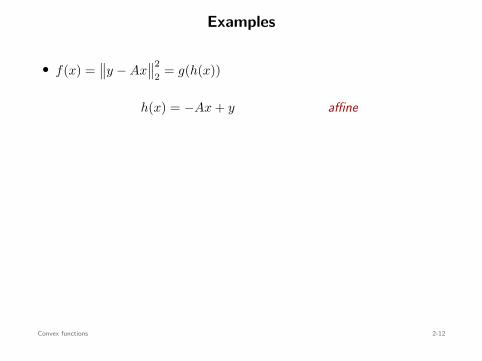
Examples
• f(x) =∥∥y − Ax
∥∥22 = g(h(x))
: convex
h(x) = −Ax + y affine
g(z) = ∥z∥22 convex
• f(x) =∥∥y − Ax
∥∥1 = g(h(x)) : convex
h(x) = −Ax + y affine
g(z) = ∥z∥1 convex
Convex functions 2-12
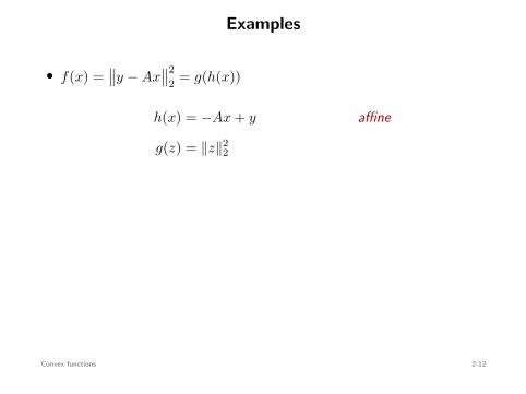
Examples
• f(x) =∥∥y − Ax
∥∥22 = g(h(x))
: convex
h(x) = −Ax + y affine
g(z) = ∥z∥22
convex
• f(x) =∥∥y − Ax
∥∥1 = g(h(x)) : convex
h(x) = −Ax + y affine
g(z) = ∥z∥1 convex
Convex functions 2-12
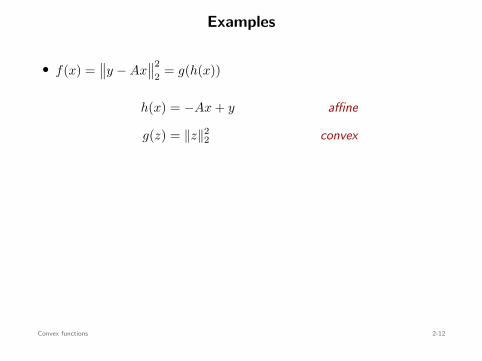
Examples
• f(x) =∥∥y − Ax
∥∥22 = g(h(x))
: convex
h(x) = −Ax + y affine
g(z) = ∥z∥22 convex
• f(x) =∥∥y − Ax
∥∥1 = g(h(x)) : convex
h(x) = −Ax + y affine
g(z) = ∥z∥1 convex
Convex functions 2-12
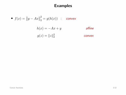
Examples
• f(x) =∥∥y − Ax
∥∥22 = g(h(x)) : convex
h(x) = −Ax + y affine
g(z) = ∥z∥22 convex
• f(x) =∥∥y − Ax
∥∥1 = g(h(x)) : convex
h(x) = −Ax + y affine
g(z) = ∥z∥1 convex
Convex functions 2-12
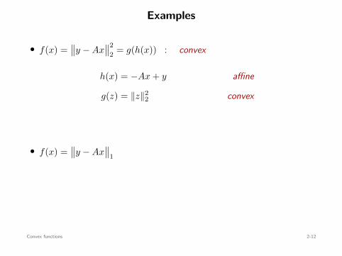
Examples
• f(x) =∥∥y − Ax
∥∥22 = g(h(x)) : convex
h(x) = −Ax + y affine
g(z) = ∥z∥22 convex
• f(x) =∥∥y − Ax
∥∥1
= g(h(x)) : convex
h(x) = −Ax + y affine
g(z) = ∥z∥1 convex
Convex functions 2-12
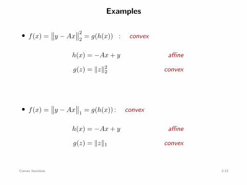
Examples
• f(x) =∥∥y − Ax
∥∥22 = g(h(x)) : convex
h(x) = −Ax + y affine
g(z) = ∥z∥22 convex
• f(x) =∥∥y − Ax
∥∥1 = g(h(x)) : convex
h(x) = −Ax + y affine
g(z) = ∥z∥1 convex
Convex functions 2-12
Outline
Convex setsIdentifying convex setsExamples: geometrical sets and filter design constraints
Convex functionsIdentifying convex functionsRelation to convex sets
Optimization problemsConvex problems, properties, and problem manipulationExamples and solvers
Statistical estimationMaximum likelihood & maximum a posterioriNonparametric estimationHypothesis testing & optimal detection
Optimization problems 3-1
Convex optimization problems
minimizex
f(x)
subject to gi(x) ≤ 0 , i = 1, . . . , m
hi(x) = 0 , i = 1, . . . , p
convex
convexaffine
Some notation
p⋆ = infx
f(x)
s.t. x ∈ Ω
∈ [−∞, +∞]
x⋆ ∈ argminx
f(x)
s.t. x ∈ Ω
Optimal value:
A minimizer:
unbounded
infeasible
Optimization problems 3-2
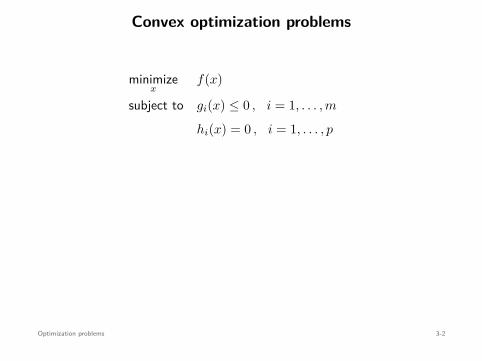
Convex optimization problems
minimizex
f(x)
subject to gi(x) ≤ 0 , i = 1, . . . , m
hi(x) = 0 , i = 1, . . . , p
convex
convexaffine
Some notation
p⋆ = infx
f(x)
s.t. x ∈ Ω
∈ [−∞, +∞]
x⋆ ∈ argminx
f(x)
s.t. x ∈ Ω
Optimal value:
A minimizer:
unbounded
infeasible
Optimization problems 3-2
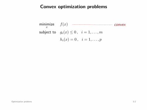
Convex optimization problems
minimizex
f(x)
subject to gi(x) ≤ 0 , i = 1, . . . , m
hi(x) = 0 , i = 1, . . . , p
convex
convexaffine
Some notation
p⋆ = infx
f(x)
s.t. x ∈ Ω
∈ [−∞, +∞]
x⋆ ∈ argminx
f(x)
s.t. x ∈ Ω
Optimal value:
A minimizer:
unbounded
infeasible
Optimization problems 3-2
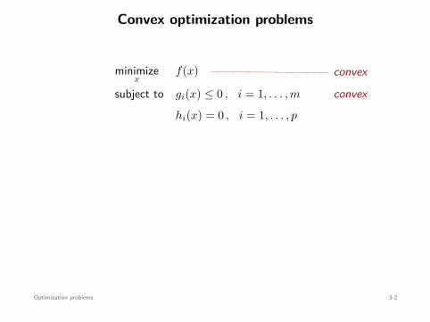
Convex optimization problems
minimizex
f(x)
subject to gi(x) ≤ 0 , i = 1, . . . , m
hi(x) = 0 , i = 1, . . . , p
convex
convex
affine
Some notation
p⋆ = infx
f(x)
s.t. x ∈ Ω
∈ [−∞, +∞]
x⋆ ∈ argminx
f(x)
s.t. x ∈ Ω
Optimal value:
A minimizer:
unbounded
infeasible
Optimization problems 3-2
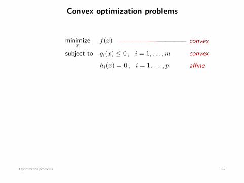
Convex optimization problems
minimizex
f(x)
subject to gi(x) ≤ 0 , i = 1, . . . , m
hi(x) = 0 , i = 1, . . . , p
convex
convexaffine
Some notation
p⋆ = infx
f(x)
s.t. x ∈ Ω
∈ [−∞, +∞]
x⋆ ∈ argminx
f(x)
s.t. x ∈ Ω
Optimal value:
A minimizer:
unbounded
infeasible
Optimization problems 3-2
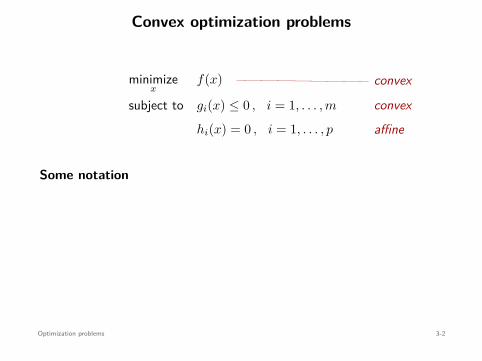
Convex optimization problems
minimizex
f(x)
subject to gi(x) ≤ 0 , i = 1, . . . , m
hi(x) = 0 , i = 1, . . . , p
convex
convexaffine
Some notation
p⋆ = infx
f(x)
s.t. x ∈ Ω
∈ [−∞, +∞]
x⋆ ∈ argminx
f(x)
s.t. x ∈ Ω
Optimal value:
A minimizer:
unbounded
infeasible
Optimization problems 3-2
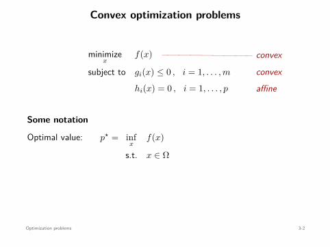
Convex optimization problems
minimizex
f(x)
subject to gi(x) ≤ 0 , i = 1, . . . , m
hi(x) = 0 , i = 1, . . . , p
convex
convexaffine
Some notation
p⋆ = infx
f(x)
s.t. x ∈ Ω
∈ [−∞, +∞]
x⋆ ∈ argminx
f(x)
s.t. x ∈ Ω
Optimal value:
A minimizer:
unbounded
infeasible
Optimization problems 3-2
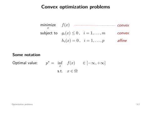
Convex optimization problems
minimizex
f(x)
subject to gi(x) ≤ 0 , i = 1, . . . , m
hi(x) = 0 , i = 1, . . . , p
convex
convexaffine
Some notation
p⋆ = infx
f(x)
s.t. x ∈ Ω
∈ [−∞, +∞]
x⋆ ∈ argminx
f(x)
s.t. x ∈ Ω
Optimal value:
A minimizer:
unbounded
infeasible
Optimization problems 3-2
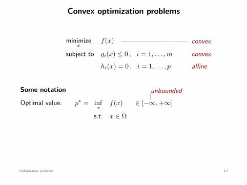
Convex optimization problems
minimizex
f(x)
subject to gi(x) ≤ 0 , i = 1, . . . , m
hi(x) = 0 , i = 1, . . . , p
convex
convexaffine
Some notation
p⋆ = infx
f(x)
s.t. x ∈ Ω
∈ [−∞, +∞]
x⋆ ∈ argminx
f(x)
s.t. x ∈ Ω
Optimal value:
A minimizer:
unbounded
infeasible
Optimization problems 3-2
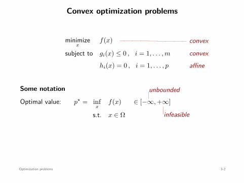
Convex optimization problems
minimizex
f(x)
subject to gi(x) ≤ 0 , i = 1, . . . , m
hi(x) = 0 , i = 1, . . . , p
convex
convexaffine
Some notation
p⋆ = infx
f(x)
s.t. x ∈ Ω
∈ [−∞, +∞]
x⋆ ∈ argminx
f(x)
s.t. x ∈ Ω
Optimal value:
A minimizer:
unbounded
infeasible
Optimization problems 3-2
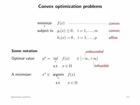
Convex optimization problems
minimizex
f(x)
subject to gi(x) ≤ 0 , i = 1, . . . , m
hi(x) = 0 , i = 1, . . . , p
convex
convexaffine
Some notation
p⋆ = infx
f(x)
s.t. x ∈ Ω
∈ [−∞, +∞]
x⋆ ∈ argminx
f(x)
s.t. x ∈ Ω
Optimal value:
A minimizer:
unbounded
infeasible
Optimization problems 3-2
Convex optimization problems
Theorem
In convex problems, a local minimizer is always a global minimizer.
Proof (for unconstrained problems w/ differentiable objective):
Recall that for any x, y ∈ dom f ,
f(y) ≥ f(x) + ∇f(x)⊤(y − x)
x⋆: local minimizer ⇒ ∇f(x⋆) = 0
Therefore, f(y) ≥ f(x⋆), for all y.
f(x) + ∇f(x)⊤(y − x)b
x
Optimization problems 3-3
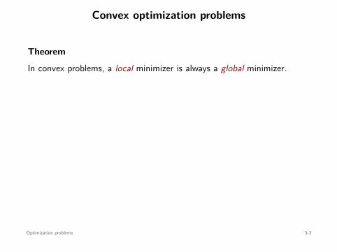
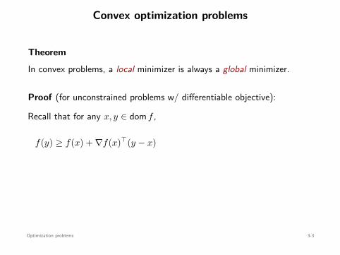
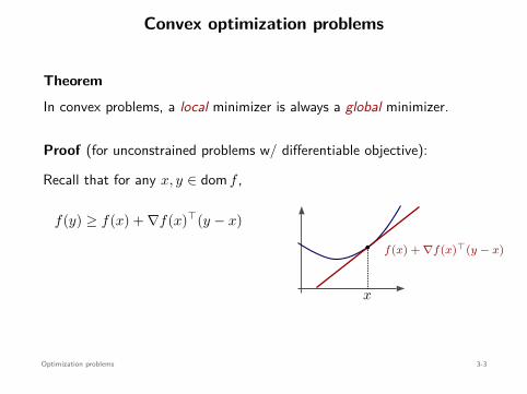
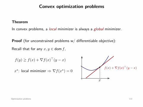
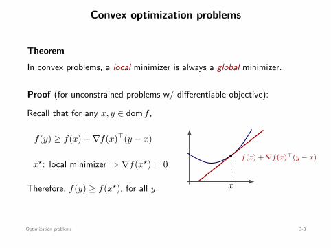

Equivalence between optimization problems
minimizex
f(x)
subject to x ∈ X
(P1)
minimizey
g(y)
subject to y ∈ Y
(P2)
(P1) and (P2) are equivalent when
• Given a solution x⋆ of (P1) we can obtain a solution y⋆ of (P2)
• Given a solution y⋆ of (P2) we can obtain a solution x⋆ of (P1)
Optimization problems 3-4
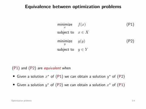

Examples
maximizex
f(x) ⇐⇒ minimizex
− f(x)
minimizex
f(x)
subject to x > 0⇐⇒ minimize
yf
(ey
)
minimizex
f(x) ⇐⇒minimize
x,tt
subject to f(x) ≤ t
Optimization problems 3-5
Examples
maximizex
f(x)
⇐⇒ minimizex
− f(x)
minimizex
f(x)
subject to x > 0⇐⇒ minimize
yf
(ey
)
minimizex
f(x) ⇐⇒minimize
x,tt
subject to f(x) ≤ t
Optimization problems 3-5
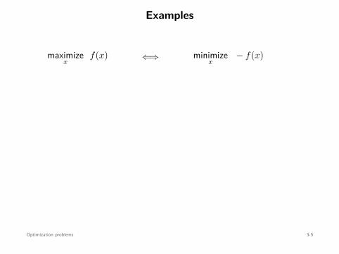
Examples
maximizex
f(x) ⇐⇒ minimizex
− f(x)
minimizex
f(x)
subject to x > 0⇐⇒ minimize
yf
(ey
)
minimizex
f(x) ⇐⇒minimize
x,tt
subject to f(x) ≤ t
Optimization problems 3-5
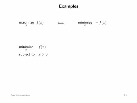
Examples
maximizex
f(x) ⇐⇒ minimizex
− f(x)
minimizex
f(x)
subject to x > 0
⇐⇒ minimizey
f(ey
)
minimizex
f(x) ⇐⇒minimize
x,tt
subject to f(x) ≤ t
Optimization problems 3-5
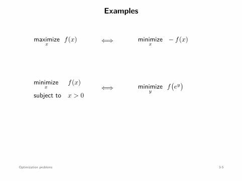
Examples
maximizex
f(x) ⇐⇒ minimizex
− f(x)
minimizex
f(x)
subject to x > 0⇐⇒ minimize
yf
(ey
)
minimizex
f(x) ⇐⇒minimize
x,tt
subject to f(x) ≤ t
Optimization problems 3-5
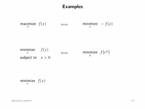
Examples
maximizex
f(x) ⇐⇒ minimizex
− f(x)
minimizex
f(x)
subject to x > 0⇐⇒ minimize
yf
(ey
)
minimizex
f(x)
⇐⇒minimize
x,tt
subject to f(x) ≤ t
Optimization problems 3-5
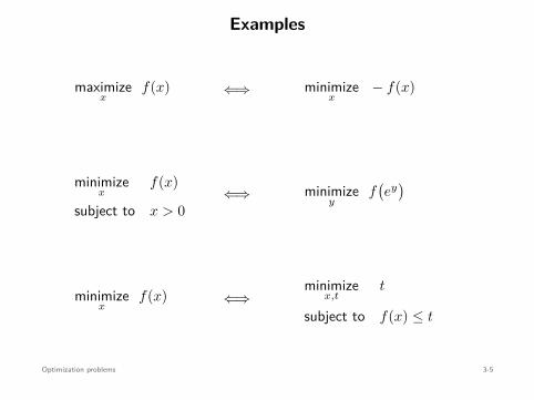
Examples
maximizex
f(x) ⇐⇒ minimizex
− f(x)
minimizex
f(x)
subject to x > 0⇐⇒ minimize
yf
(ey
)
minimizex
f(x) ⇐⇒minimize
x,tt
subject to f(x) ≤ t
Optimization problems 3-5

Examples
minimizex
a f(x) + b
> 0
⇐⇒ minimizex
f(x)
minimizex
f(x)
convex
⇐⇒ minimizex
g(f(x)
)
if im f ⊆ dom g
and g f : convex
Optimization problems 3-6
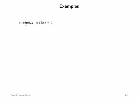
Examples
minimizex
a f(x) + b
> 0
⇐⇒ minimizex
f(x)
minimizex
f(x)
convex
⇐⇒ minimizex
g(f(x)
)
if im f ⊆ dom g
and g f : convex
Optimization problems 3-6
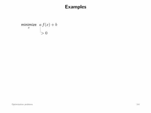
Examples
minimizex
a f(x) + b
> 0
⇐⇒ minimizex
f(x)
minimizex
f(x)
convex
⇐⇒ minimizex
g(f(x)
)
if im f ⊆ dom g
and g f : convex
Optimization problems 3-6
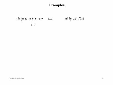
Examples
minimizex
a f(x) + b
> 0
⇐⇒ minimizex
f(x)
minimizex
f(x)
convex
⇐⇒ minimizex
g(f(x)
)
if im f ⊆ dom g
and g f : convex
Optimization problems 3-6
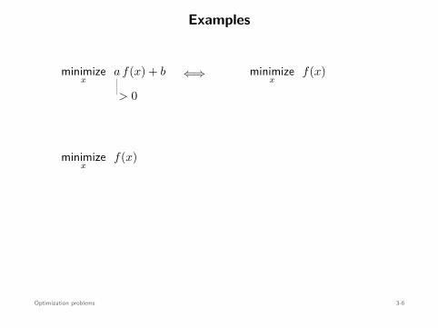
Examples
minimizex
a f(x) + b
> 0
⇐⇒ minimizex
f(x)
minimizex
f(x)
convex
⇐⇒ minimizex
g(f(x)
)
if im f ⊆ dom g
and g f : convex
Optimization problems 3-6
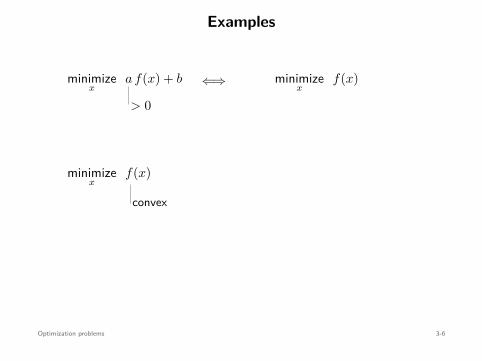
Examples
minimizex
a f(x) + b
> 0
⇐⇒ minimizex
f(x)
minimizex
f(x)
convex
⇐⇒ minimizex
g(f(x)
)
if im f ⊆ dom g
and g f : convex
Optimization problems 3-6
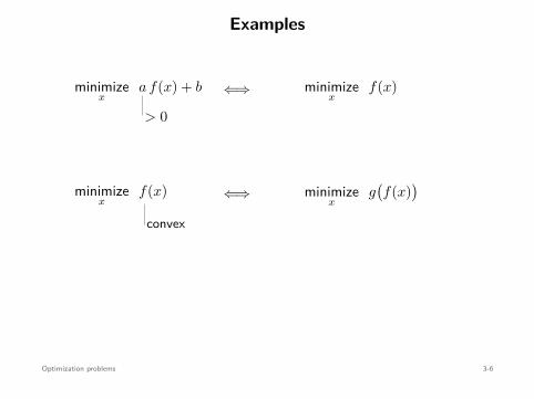
Examples
minimizex
a f(x) + b
> 0
⇐⇒ minimizex
f(x)
minimizex
f(x)
convex
⇐⇒ minimizex
g(f(x)
)
if im f ⊆ dom g
and g f : convex
Optimization problems 3-6
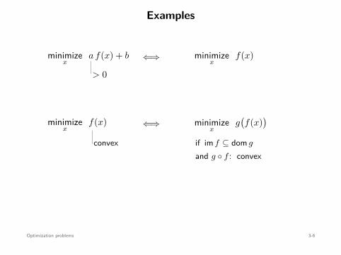
Examples
minimizex
a f(x) + b
> 0
⇐⇒ minimizex
f(x)
minimizex
f(x)
convex
⇐⇒ minimizex
g(f(x)
)
if im f ⊆ dom g
and g f : convex
Optimization problems 3-6

Air Traffic Control
• n airplanes land in order 1, 2, . . . , n
• ti: arrival time of airplane i
• Airplane i has to land in interval [mi, Mi]
m1 M1 m2 M2 m3 M3 m4 M4
tt1 t2 t3 t4
mini
ti+1 − ti
Goal: compute t1, . . . , tn that maximize mini ti+1 − ti
Optimization problems 3-7

Air Traffic Control
• n airplanes land in order 1, 2, . . . , n
• ti: arrival time of airplane i
• Airplane i has to land in interval [mi, Mi]
m1 M1 m2 M2 m3 M3 m4 M4
tt1 t2 t3 t4
mini
ti+1 − ti
Goal: compute t1, . . . , tn that maximize mini ti+1 − ti
Optimization problems 3-7

Air Traffic Control
• n airplanes land in order 1, 2, . . . , n
• ti: arrival time of airplane i
• Airplane i has to land in interval [mi, Mi]
m1 M1 m2 M2 m3 M3 m4 M4
t
t1 t2 t3 t4
mini
ti+1 − ti
Goal: compute t1, . . . , tn that maximize mini ti+1 − ti
Optimization problems 3-7

Air Traffic Control
• n airplanes land in order 1, 2, . . . , n
• ti: arrival time of airplane i
• Airplane i has to land in interval [mi, Mi]
m1 M1 m2 M2 m3 M3 m4 M4
t
t1 t2 t3 t4
mini
ti+1 − ti
Goal: compute t1, . . . , tn that maximize mini ti+1 − ti
Optimization problems 3-7
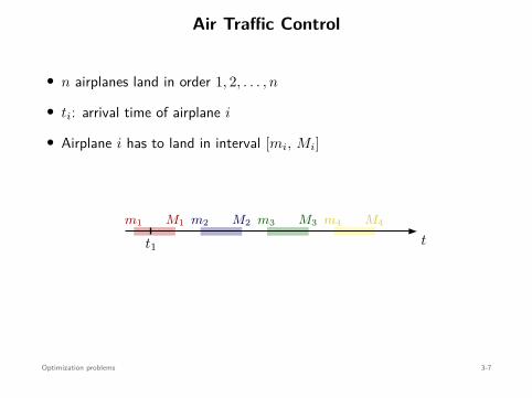
Air Traffic Control
• n airplanes land in order 1, 2, . . . , n
• ti: arrival time of airplane i
• Airplane i has to land in interval [mi, Mi]
m1 M1 m2 M2 m3 M3 m4 M4
tt1
t2 t3 t4
mini
ti+1 − ti
Goal: compute t1, . . . , tn that maximize mini ti+1 − ti
Optimization problems 3-7
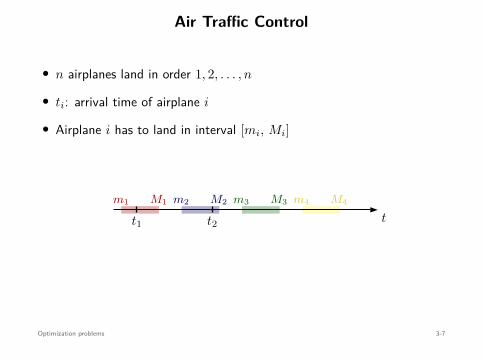
Air Traffic Control
• n airplanes land in order 1, 2, . . . , n
• ti: arrival time of airplane i
• Airplane i has to land in interval [mi, Mi]
m1 M1 m2 M2 m3 M3 m4 M4
tt1 t2
t3 t4
mini
ti+1 − ti
Goal: compute t1, . . . , tn that maximize mini ti+1 − ti
Optimization problems 3-7
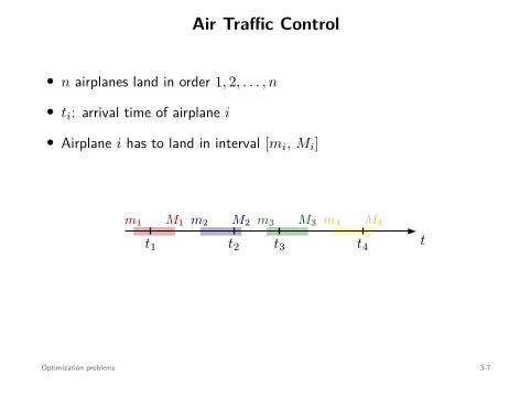
Air Traffic Control
• n airplanes land in order 1, 2, . . . , n
• ti: arrival time of airplane i
• Airplane i has to land in interval [mi, Mi]
m1 M1 m2 M2 m3 M3 m4 M4
tt1 t2 t3 t4
mini
ti+1 − ti
Goal: compute t1, . . . , tn that maximize mini ti+1 − ti
Optimization problems 3-7
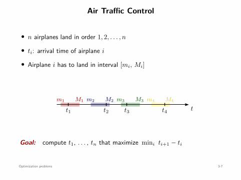
Air Traffic Control
• n airplanes land in order 1, 2, . . . , n
• ti: arrival time of airplane i
• Airplane i has to land in interval [mi, Mi]
m1 M1 m2 M2 m3 M3 m4 M4
tt1 t2 t3 t4
mini
ti+1 − ti
Goal: compute t1, . . . , tn that maximize mini ti+1 − ti
Optimization problems 3-7
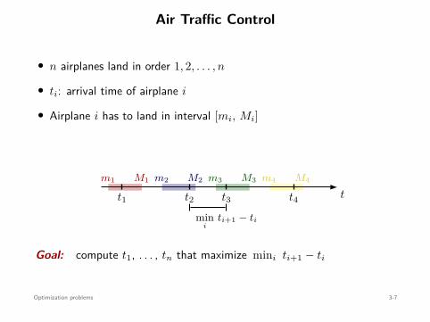
Air Traffic Control
• n airplanes land in order 1, 2, . . . , n
• ti: arrival time of airplane i
• Airplane i has to land in interval [mi, Mi]
m1 M1 m2 M2 m3 M3 m4 M4
tt1 t2 t3 t4
mini
ti+1 − ti
Goal: compute t1, . . . , tn that maximize mini ti+1 − ti
Optimization problems 3-7
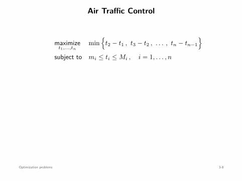
Air Traffic Control
maximizet1,...,tn
min
t2 − t1 , t3 − t2 , . . . , tn − tn−1
subject to mi ≤ ti ≤ Mi , i = 1, . . . , n
⇐⇒ minimizet1,...,tn
− min
t2 − t1 , t3 − t2 , . . . , tn − tn−1
subject to mi ≤ ti ≤ Mi , i = 1, . . . , n
⇐⇒ minimizet1,...,tn
max
t1 − t2 , t2 − t3 , . . . , tn−1 − tn
subject to mi ≤ ti ≤ Mi , i = 1, . . . , n
Convex
Optimization problems 3-8
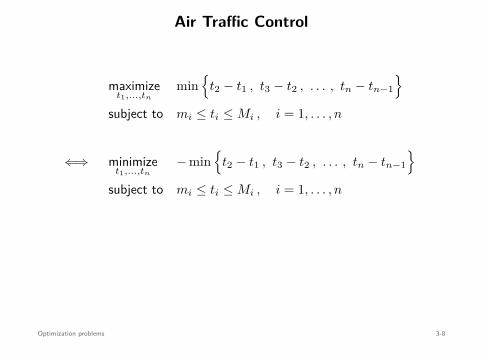
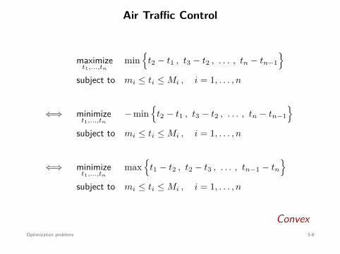
Air Traffic Control
maximizet1,...,tn
min
t2 − t1 , t3 − t2 , . . . , tn − tn−1
subject to mi ≤ ti ≤ Mi , i = 1, . . . , n
⇐⇒ minimizet1,...,tn
− min
t2 − t1 , t3 − t2 , . . . , tn − tn−1
subject to mi ≤ ti ≤ Mi , i = 1, . . . , n
⇐⇒ minimizet1,...,tn
max
t1 − t2 , t2 − t3 , . . . , tn−1 − tn
subject to mi ≤ ti ≤ Mi , i = 1, . . . , n
ConvexOptimization problems 3-8
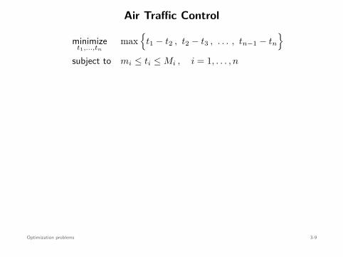
Air Traffic Control
minimizet1,...,tn
max
t1 − t2 , t2 − t3 , . . . , tn−1 − tn
subject to mi ≤ ti ≤ Mi , i = 1, . . . , n
⇐⇒ minimizet1,...,tn,s
s
subject to max
t1 − t2 , t2 − t3 , . . . , tn−1 − tn
≤ s
mi ≤ ti ≤ Mi , i = 1, . . . , n
⇐⇒ minimizet1,...,tn,s
s
subject to t1 − t2 ≤ s...
tn−1 − tn ≤ s
mi ≤ ti ≤ Mi , i = 1, . . . , n
Optimization problems 3-9
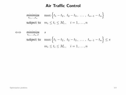
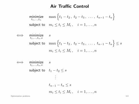
Air Traffic Control
minimizet1,...,tn
max
t1 − t2 , t2 − t3 , . . . , tn−1 − tn
subject to mi ≤ ti ≤ Mi , i = 1, . . . , n
⇐⇒ minimizet1,...,tn,s
s
subject to max
t1 − t2 , t2 − t3 , . . . , tn−1 − tn
≤ s
mi ≤ ti ≤ Mi , i = 1, . . . , n
⇐⇒ minimizet1,...,tn,s
s
subject to t1 − t2 ≤ s...
tn−1 − tn ≤ s
mi ≤ ti ≤ Mi , i = 1, . . . , nOptimization problems 3-9

Air Traffic ControlThis is a linear program (LP):
minimizex
c⊤x
subject to Ax ≤ b
with x = (t1, . . . , tn, s) ∈ Rn+1, c = (0, · · · , 0, 1), and
A =
1 −1 0 · · · 0 0 −10 1 −1 · · · 0 0 −1
. . .
0 0 0 · · · 1 −1 −1−1 0 0 · · · 0 0 0
1 0 0 · · · 0 0 0. . .
0 0 0 · · · 0 −1 00 0 0 · · · 0 1 0
b =
00...0
−m1
M1
...−mn
Mn
Optimization problems 3-10
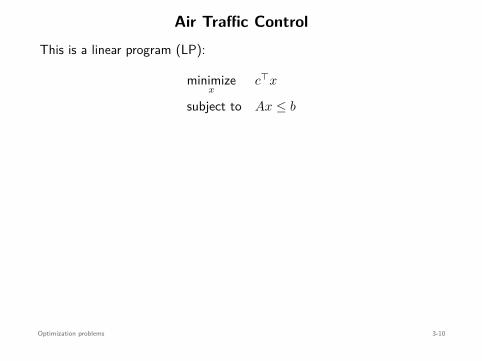
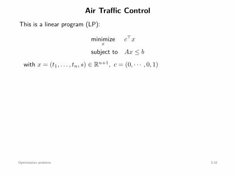
Air Traffic ControlThis is a linear program (LP):
minimizex
c⊤x
subject to Ax ≤ b
with x = (t1, . . . , tn, s) ∈ Rn+1, c = (0, · · · , 0, 1)
, and
A =
1 −1 0 · · · 0 0 −10 1 −1 · · · 0 0 −1
. . .
0 0 0 · · · 1 −1 −1−1 0 0 · · · 0 0 0
1 0 0 · · · 0 0 0. . .
0 0 0 · · · 0 −1 00 0 0 · · · 0 1 0
b =
00...0
−m1
M1
...−mn
Mn
Optimization problems 3-10
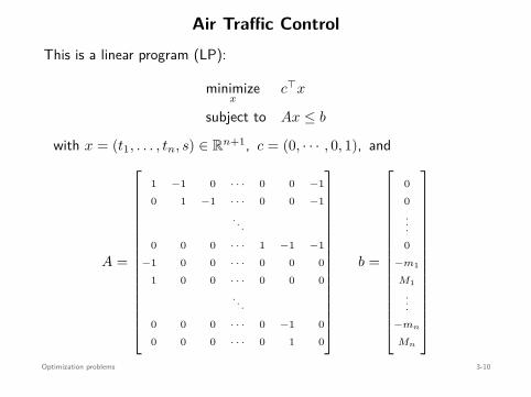
Air Traffic ControlThis is a linear program (LP):
minimizex
c⊤x
subject to Ax ≤ b
with x = (t1, . . . , tn, s) ∈ Rn+1, c = (0, · · · , 0, 1), and
A =
1 −1 0 · · · 0 0 −10 1 −1 · · · 0 0 −1
. . .
0 0 0 · · · 1 −1 −1−1 0 0 · · · 0 0 0
1 0 0 · · · 0 0 0. . .
0 0 0 · · · 0 −1 00 0 0 · · · 0 1 0
b =
00...0
−m1
M1
...−mn
Mn
Optimization problems 3-10

Air Traffic Control
Can be solved, e.g., with MATLAB’s linprog solver
But we have to explicitly construct A, b, and c . . .
CVX (cvxr.com/cvx) manipulates and solves convex problems
Optimization problems 3-11

Air Traffic Control
Can be solved, e.g., with MATLAB’s linprog solver
But we have to explicitly construct A, b, and c . . .
CVX (cvxr.com/cvx) manipulates and solves convex problems
Optimization problems 3-11

Air Traffic Control
Can be solved, e.g., with MATLAB’s linprog solver
But we have to explicitly construct A, b, and c . . .
CVX (cvxr.com/cvx) manipulates and solves convex problems
Optimization problems 3-11

Air Traffic Control
cvx_beg inv a r i a b l e s t1 t2 t3 t4 t5 ;maximize ( min ( [ t2−t1 , t3−t2 , t4−t3 , t5−t4 ] ) ) ;s u b j e c t to
1 <= t1 <= 2 ;3 <= t2 <= 4 ;5 <= t3 <= 6 ;7 <= t4 <= 8 ;9 <= t5 <= 10 ;
cvx_end
(t⋆1 , t⋆
2 , t⋆3 , t⋆
4 , t⋆5) = (1 , 3.25 , 5.5 , 7.75 , 10)
Optimization problems 3-12
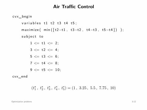

Portfolio Optimization
• £T to invest in n assets• ri: return of asset i, for i = 1, . . . , n (random variables)• First two moments of the random vector r = (r1, . . . , rn) are known:
µ = E[r] Σ = E[(r − µ)(r − µ)⊤]
• An investment x = (x1, . . . , xn) has return
s(x) = r⊤x = r1x1 + · · · + rnxn
E[s(x)
]= E[r1] x1 + · · · + E[rn] xn = µ1 x1 + · · · + µn xn = µ⊤x
Var(s(x)
)= E
[(s(x) − E[s(x)]
)2]
= E[(
(r − µ)⊤x)2
]= x⊤Σ x
Optimization problems 3-13

Portfolio Optimization
• £T to invest in n assets
• ri: return of asset i, for i = 1, . . . , n (random variables)• First two moments of the random vector r = (r1, . . . , rn) are known:
µ = E[r] Σ = E[(r − µ)(r − µ)⊤]
• An investment x = (x1, . . . , xn) has return
s(x) = r⊤x = r1x1 + · · · + rnxn
E[s(x)
]= E[r1] x1 + · · · + E[rn] xn = µ1 x1 + · · · + µn xn = µ⊤x
Var(s(x)
)= E
[(s(x) − E[s(x)]
)2]
= E[(
(r − µ)⊤x)2
]= x⊤Σ x
Optimization problems 3-13

Portfolio Optimization
• £T to invest in n assets• ri: return of asset i, for i = 1, . . . , n (random variables)
• First two moments of the random vector r = (r1, . . . , rn) are known:
µ = E[r] Σ = E[(r − µ)(r − µ)⊤]
• An investment x = (x1, . . . , xn) has return
s(x) = r⊤x = r1x1 + · · · + rnxn
E[s(x)
]= E[r1] x1 + · · · + E[rn] xn = µ1 x1 + · · · + µn xn = µ⊤x
Var(s(x)
)= E
[(s(x) − E[s(x)]
)2]
= E[(
(r − µ)⊤x)2
]= x⊤Σ x
Optimization problems 3-13

Portfolio Optimization
• £T to invest in n assets• ri: return of asset i, for i = 1, . . . , n (random variables)• First two moments of the random vector r = (r1, . . . , rn) are known:
µ = E[r] Σ = E[(r − µ)(r − µ)⊤]
• An investment x = (x1, . . . , xn) has return
s(x) = r⊤x = r1x1 + · · · + rnxn
E[s(x)
]= E[r1] x1 + · · · + E[rn] xn = µ1 x1 + · · · + µn xn = µ⊤x
Var(s(x)
)= E
[(s(x) − E[s(x)]
)2]
= E[(
(r − µ)⊤x)2
]= x⊤Σ x
Optimization problems 3-13
Portfolio Optimization
• £T to invest in n assets• ri: return of asset i, for i = 1, . . . , n (random variables)• First two moments of the random vector r = (r1, . . . , rn) are known:
µ = E[r] Σ = E[(r − µ)(r − µ)⊤]
• An investment x = (x1, . . . , xn) has return
s(x) = r⊤x = r1x1 + · · · + rnxn
E[s(x)
]
= E[r1] x1 + · · · + E[rn] xn = µ1 x1 + · · · + µn xn = µ⊤x
Var(s(x)
)= E
[(s(x) − E[s(x)]
)2]
= E[(
(r − µ)⊤x)2
]= x⊤Σ x
Optimization problems 3-13
Portfolio Optimization
• £T to invest in n assets• ri: return of asset i, for i = 1, . . . , n (random variables)• First two moments of the random vector r = (r1, . . . , rn) are known:
µ = E[r] Σ = E[(r − µ)(r − µ)⊤]
• An investment x = (x1, . . . , xn) has return
s(x) = r⊤x = r1x1 + · · · + rnxn
E[s(x)
]= E[r1] x1 + · · · + E[rn] xn
= µ1 x1 + · · · + µn xn = µ⊤x
Var(s(x)
)= E
[(s(x) − E[s(x)]
)2]
= E[(
(r − µ)⊤x)2
]= x⊤Σ x
Optimization problems 3-13

Portfolio Optimization
• £T to invest in n assets• ri: return of asset i, for i = 1, . . . , n (random variables)• First two moments of the random vector r = (r1, . . . , rn) are known:
µ = E[r] Σ = E[(r − µ)(r − µ)⊤]
• An investment x = (x1, . . . , xn) has return
s(x) = r⊤x = r1x1 + · · · + rnxn
E[s(x)
]= E[r1] x1 + · · · + E[rn] xn = µ1 x1 + · · · + µn xn
= µ⊤x
Var(s(x)
)= E
[(s(x) − E[s(x)]
)2]
= E[(
(r − µ)⊤x)2
]= x⊤Σ x
Optimization problems 3-13
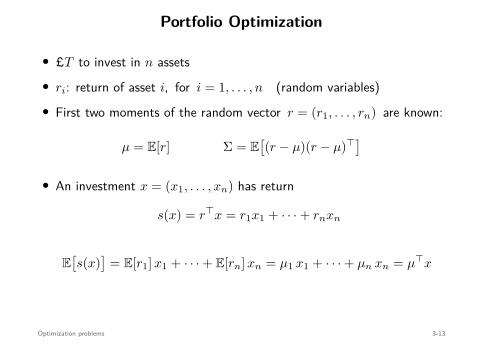
Portfolio Optimization
• £T to invest in n assets• ri: return of asset i, for i = 1, . . . , n (random variables)• First two moments of the random vector r = (r1, . . . , rn) are known:
µ = E[r] Σ = E[(r − µ)(r − µ)⊤]
• An investment x = (x1, . . . , xn) has return
s(x) = r⊤x = r1x1 + · · · + rnxn
E[s(x)
]= E[r1] x1 + · · · + E[rn] xn = µ1 x1 + · · · + µn xn = µ⊤x
Var(s(x)
)= E
[(s(x) − E[s(x)]
)2]
= E[(
(r − µ)⊤x)2
]= x⊤Σ x
Optimization problems 3-13
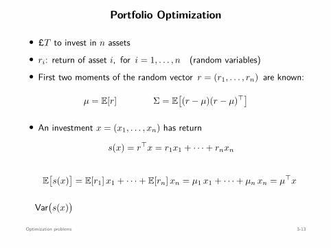
Portfolio Optimization
• £T to invest in n assets• ri: return of asset i, for i = 1, . . . , n (random variables)• First two moments of the random vector r = (r1, . . . , rn) are known:
µ = E[r] Σ = E[(r − µ)(r − µ)⊤]
• An investment x = (x1, . . . , xn) has return
s(x) = r⊤x = r1x1 + · · · + rnxn
E[s(x)
]= E[r1] x1 + · · · + E[rn] xn = µ1 x1 + · · · + µn xn = µ⊤x
Var(s(x)
)
= E[(
s(x) − E[s(x)])2
]= E
[((r − µ)⊤x
)2]
= x⊤Σ x
Optimization problems 3-13
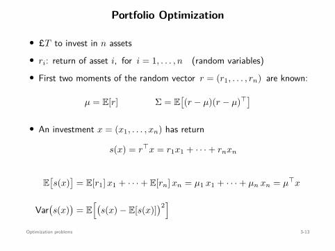
Portfolio Optimization
• £T to invest in n assets• ri: return of asset i, for i = 1, . . . , n (random variables)• First two moments of the random vector r = (r1, . . . , rn) are known:
µ = E[r] Σ = E[(r − µ)(r − µ)⊤]
• An investment x = (x1, . . . , xn) has return
s(x) = r⊤x = r1x1 + · · · + rnxn
E[s(x)
]= E[r1] x1 + · · · + E[rn] xn = µ1 x1 + · · · + µn xn = µ⊤x
Var(s(x)
)= E
[(s(x) − E[s(x)]
)2]
= E[(
(r − µ)⊤x)2
]= x⊤Σ x
Optimization problems 3-13
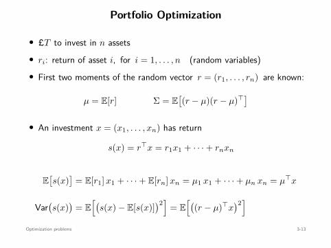
Portfolio Optimization
• £T to invest in n assets• ri: return of asset i, for i = 1, . . . , n (random variables)• First two moments of the random vector r = (r1, . . . , rn) are known:
µ = E[r] Σ = E[(r − µ)(r − µ)⊤]
• An investment x = (x1, . . . , xn) has return
s(x) = r⊤x = r1x1 + · · · + rnxn
E[s(x)
]= E[r1] x1 + · · · + E[rn] xn = µ1 x1 + · · · + µn xn = µ⊤x
Var(s(x)
)= E
[(s(x) − E[s(x)]
)2]
= E[(
(r − µ)⊤x)2
]
= x⊤Σ x
Optimization problems 3-13
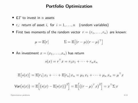
Portfolio Optimization
• £T to invest in n assets• ri: return of asset i, for i = 1, . . . , n (random variables)• First two moments of the random vector r = (r1, . . . , rn) are known:
µ = E[r] Σ = E[(r − µ)(r − µ)⊤]
• An investment x = (x1, . . . , xn) has return
s(x) = r⊤x = r1x1 + · · · + rnxn
E[s(x)
]= E[r1] x1 + · · · + E[rn] xn = µ1 x1 + · · · + µn xn = µ⊤x
Var(s(x)
)= E
[(s(x) − E[s(x)]
)2]
= E[(
(r − µ)⊤x)2
]= x⊤Σ x
Optimization problems 3-13

Portfolio Optimization
Different investment strategies
• Minimize variance while guaranteeing minimum expected return smin:
minimizex
Var(s(x)
)
subject to x ≥ 0n
1⊤n x = T
E[s(x)
]≥ smin
⇐⇒ minimizex
x⊤Σx
subject to x ≥ 0n
1⊤n x = T
µ⊤x ≥ smin
Convex Quadratic Program (QP)
Optimization problems 3-14
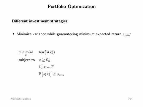
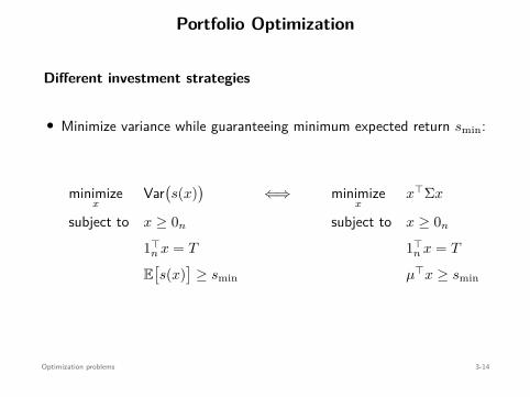
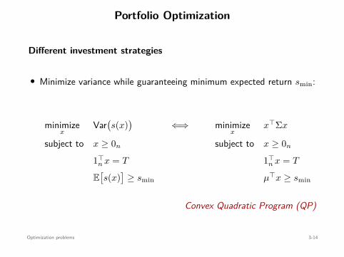
Portfolio Optimization
• Maximize expected return with risk penalty β ≥ 0:
maximizex
E[s(x)
]− β Var(s(x))
subject to x ≥ 0n
1⊤n x = T
⇐⇒ minimizex
−µ⊤x + β x⊤Σ x
subject to x ≥ 0n
1⊤n x = T
Convex QP
Optimization problems 3-15
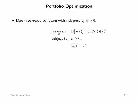
Portfolio Optimization
• Maximize expected return with risk penalty β ≥ 0:
maximizex
E[s(x)
]− β Var(s(x))
subject to x ≥ 0n
1⊤n x = T
⇐⇒ minimizex
−µ⊤x + β x⊤Σ x
subject to x ≥ 0n
1⊤n x = T
Convex QP
Optimization problems 3-15
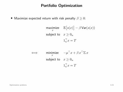
Portfolio Optimization
• Maximize expected return with risk penalty β ≥ 0:
maximizex
E[s(x)
]− β Var(s(x))
subject to x ≥ 0n
1⊤n x = T
⇐⇒ minimizex
−µ⊤x + β x⊤Σ x
subject to x ≥ 0n
1⊤n x = T
Convex QP
Optimization problems 3-15
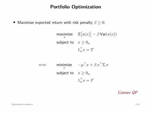
Portfolio Optimization
• Maximize expected return with risk penalty β ≥ 0:
maximizex
E[s(x)
]− β Var(s(x))
subject to x ≥ 0n
1⊤n x = T
⇐⇒ minimizex
−µ⊤x + β x⊤Σ x
subject to x ≥ 0n
1⊤n x = T
Convex QP
Optimization problems 3-15
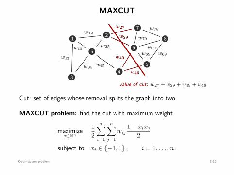
MAXCUT
1 2
34
5
6
7
89
w12
w13
w15w25
w35 w45
w69 w68
w78
w79
w89
w27
w29
w49
w46
w27
w29
w49
w46
value of cut: w27 + w29 + w49 + w46
Cut: set of edges whose removal splits the graph into two
MAXCUT problem: find the cut with maximum weight
maximizex∈Rn
12
n∑
i=1
n∑
j=1wij
1 − xixj
2
subject to xi ∈ −1, 1 , i = 1, . . . , n .
Optimization problems 3-16
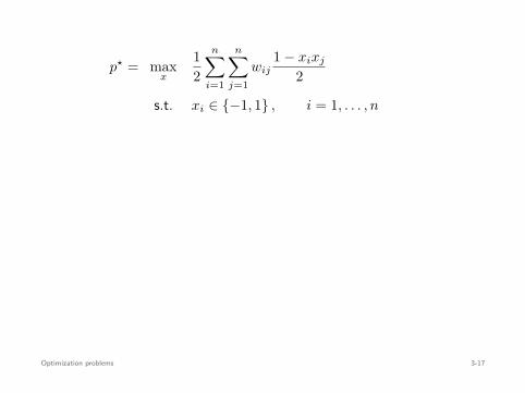
p⋆ = maxx
12
n∑
i=1
n∑
j=1wij
1 − xixj
2
s.t. xi ∈ −1, 1 , i = 1, . . . , n
= − minx
14
[n∑
i=1
n∑
j=1wijxixj −
n∑
i=1
n∑
j=1wij
]
s.t. x2i = 1 , i = 1, . . . , n
= − minx
14
(x⊤Wx − 1⊤
n W1n
)
s.t. x2i = 1 , i = 1, . . . , n
W ∈ Rn×n: weighted adjacency matrix
Optimization problems 3-17
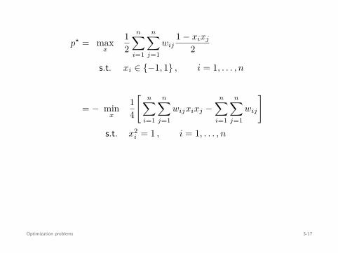
p⋆ = maxx
12
n∑
i=1
n∑
j=1wij
1 − xixj
2
s.t. xi ∈ −1, 1 , i = 1, . . . , n
= − minx
14
[n∑
i=1
n∑
j=1wijxixj −
n∑
i=1
n∑
j=1wij
]
s.t. x2i = 1 , i = 1, . . . , n
= − minx
14
(x⊤Wx − 1⊤
n W1n
)
s.t. x2i = 1 , i = 1, . . . , n
W ∈ Rn×n: weighted adjacency matrix
Optimization problems 3-17
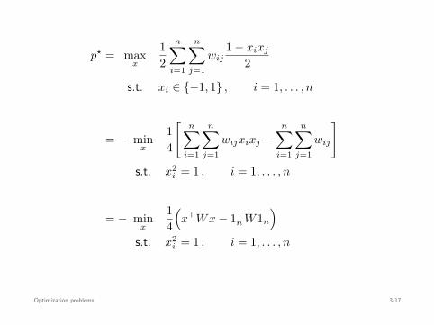
p⋆ = maxx
12
n∑
i=1
n∑
j=1wij
1 − xixj
2
s.t. xi ∈ −1, 1 , i = 1, . . . , n
= − minx
14
[n∑
i=1
n∑
j=1wijxixj −
n∑
i=1
n∑
j=1wij
]
s.t. x2i = 1 , i = 1, . . . , n
= − minx
14
(x⊤Wx − 1⊤
n W1n
)
s.t. x2i = 1 , i = 1, . . . , n
W ∈ Rn×n: weighted adjacency matrix
Optimization problems 3-17
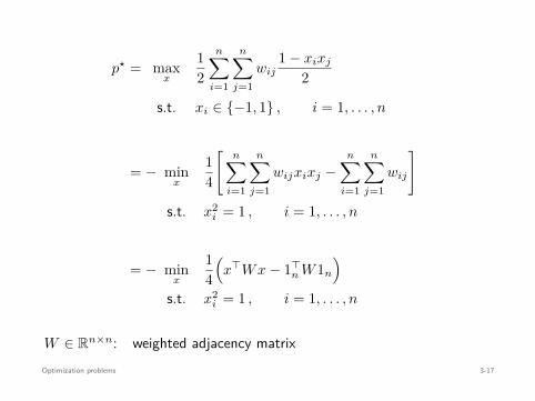
p⋆ = maxx
12
n∑
i=1
n∑
j=1wij
1 − xixj
2
s.t. xi ∈ −1, 1 , i = 1, . . . , n
= − minx
14
[n∑
i=1
n∑
j=1wijxixj −
n∑
i=1
n∑
j=1wij
]
s.t. x2i = 1 , i = 1, . . . , n
= − minx
14
(x⊤Wx − 1⊤
n W1n
)
s.t. x2i = 1 , i = 1, . . . , n
W ∈ Rn×n: weighted adjacency matrixOptimization problems 3-17
−p⋆ = minx
14
(x⊤Wx − 1⊤
n W1n
)
s.t. x2i = 1 , i = 1, . . . , n
• x⊤Wx = tr(x⊤Wx
)= tr
(Wxx⊤)
• For any X ∈ Sn and x ∈ Rn, X = xx⊤ ⇐⇒
X ⪰ 0
rank(X) = 1
−p⋆ = minX∈Sn
14
(tr
(WX
)− 1⊤
n W1n
)
s.t. Xii = 1 , i = 1, . . . , n
X ⪰ 0
rank(X) = 1 nonconvex
Optimization problems 3-18
−p⋆ = minx
14
(x⊤Wx − 1⊤
n W1n
)
s.t. x2i = 1 , i = 1, . . . , n
• x⊤Wx = tr(x⊤Wx
)= tr
(Wxx⊤)
• For any X ∈ Sn and x ∈ Rn, X = xx⊤ ⇐⇒
X ⪰ 0
rank(X) = 1
−p⋆ = minX∈Sn
14
(tr
(WX
)− 1⊤
n W1n
)
s.t. Xii = 1 , i = 1, . . . , n
X ⪰ 0
rank(X) = 1 nonconvex
Optimization problems 3-18
−p⋆ = minx
14
(x⊤Wx − 1⊤
n W1n
)
s.t. x2i = 1 , i = 1, . . . , n
• x⊤Wx = tr(x⊤Wx
)= tr
(Wxx⊤)
• For any X ∈ Sn and x ∈ Rn, X = xx⊤ ⇐⇒
X ⪰ 0
rank(X) = 1
−p⋆ = minX∈Sn
14
(tr
(WX
)− 1⊤
n W1n
)
s.t. Xii = 1 , i = 1, . . . , n
X ⪰ 0
rank(X) = 1 nonconvex
Optimization problems 3-18
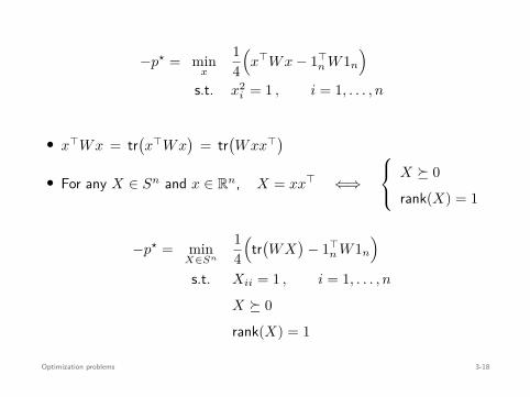
−p⋆ = minx
14
(x⊤Wx − 1⊤
n W1n
)
s.t. x2i = 1 , i = 1, . . . , n
• x⊤Wx = tr(x⊤Wx
)= tr
(Wxx⊤)
• For any X ∈ Sn and x ∈ Rn, X = xx⊤ ⇐⇒
X ⪰ 0
rank(X) = 1
−p⋆ = minX∈Sn
14
(tr
(WX
)− 1⊤
n W1n
)
s.t. Xii = 1 , i = 1, . . . , n
X ⪰ 0
rank(X) = 1
nonconvex
Optimization problems 3-18
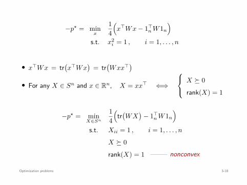
−p⋆ = minx
14
(x⊤Wx − 1⊤
n W1n
)
s.t. x2i = 1 , i = 1, . . . , n
• x⊤Wx = tr(x⊤Wx
)= tr
(Wxx⊤)
• For any X ∈ Sn and x ∈ Rn, X = xx⊤ ⇐⇒
X ⪰ 0
rank(X) = 1
−p⋆ = minX∈Sn
14
(tr
(WX
)− 1⊤
n W1n
)
s.t. Xii = 1 , i = 1, . . . , n
X ⪰ 0
rank(X) = 1 nonconvex
Optimization problems 3-18
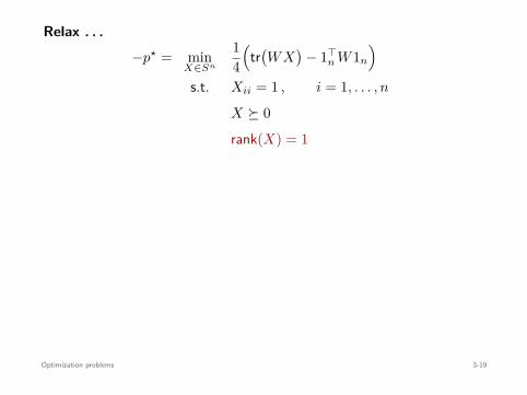
Relax . . .−p⋆ = min
X∈Sn
14
(tr
(WX
)− 1⊤
n W1n
)
s.t. Xii = 1 , i = 1, . . . , n
X ⪰ 0
rank(X) = 1
≥ minX∈Sn
14
(tr
(WX
)− 1⊤
n W1n
)
s.t. Xii = 1 , i = 1, . . . , n
X ⪰ 0
=: −d⋆
Convex Semi-Definite Program (SDP)
Optimization problems 3-19
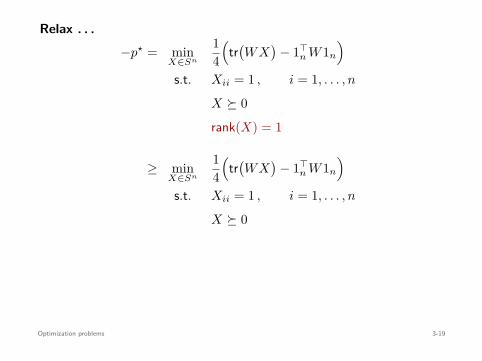
Relax . . .−p⋆ = min
X∈Sn
14
(tr
(WX
)− 1⊤
n W1n
)
s.t. Xii = 1 , i = 1, . . . , n
X ⪰ 0
rank(X) = 1
≥ minX∈Sn
14
(tr
(WX
)− 1⊤
n W1n
)
s.t. Xii = 1 , i = 1, . . . , n
X ⪰ 0
=: −d⋆
Convex Semi-Definite Program (SDP)
Optimization problems 3-19
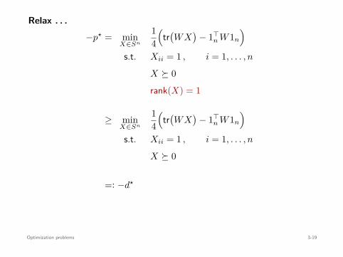
Relax . . .−p⋆ = min
X∈Sn
14
(tr
(WX
)− 1⊤
n W1n
)
s.t. Xii = 1 , i = 1, . . . , n
X ⪰ 0
rank(X) = 1
≥ minX∈Sn
14
(tr
(WX
)− 1⊤
n W1n
)
s.t. Xii = 1 , i = 1, . . . , n
X ⪰ 0
=: −d⋆
Convex Semi-Definite Program (SDP)
Optimization problems 3-19
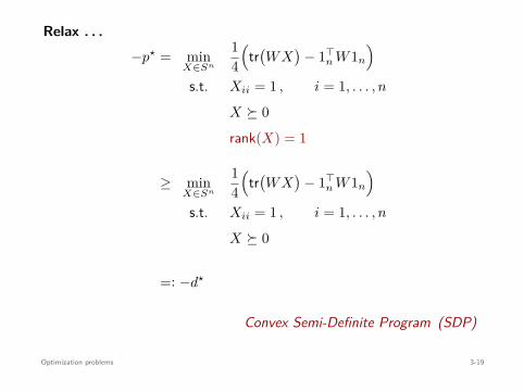
Relax . . .−p⋆ = min
X∈Sn
14
(tr
(WX
)− 1⊤
n W1n
)
s.t. Xii = 1 , i = 1, . . . , n
X ⪰ 0
rank(X) = 1
≥ minX∈Sn
14
(tr
(WX
)− 1⊤
n W1n
)
s.t. Xii = 1 , i = 1, . . . , n
X ⪰ 0
=: −d⋆
Convex Semi-Definite Program (SDP)
Optimization problems 3-19

Procedure: (Goemans & Williamson, 95’)
• Solve SDP, obtaining X⋆
• Factorize X⋆ = V ⊤V , where V =[v1 v2 · · · vn
]
• Draw r uniformly at random from unit-sphere
x ∈ Rn : ∥x∥2 = 1
• The following sets define a cut C on the vertices of the graph:
S =
i : r⊤vi ≥ 0
Sc =
i : r⊤vi < 0
It can be shown that
d⋆ ≥ p⋆ ≥ E[C] ≥ 0.87856 d⋆
Optimization problems 3-20
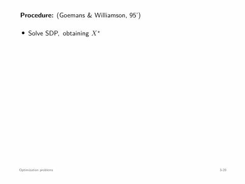
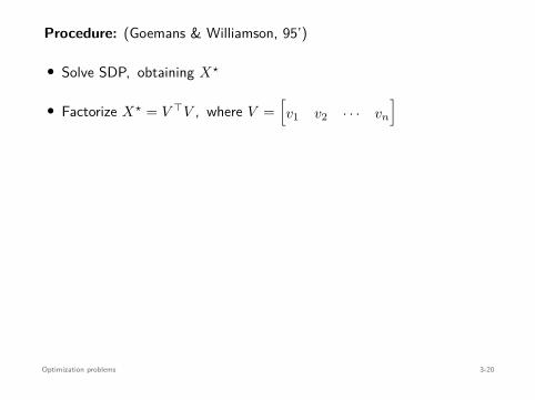
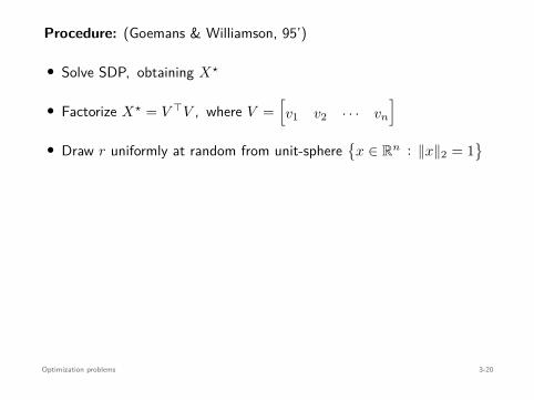
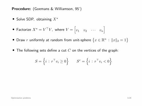
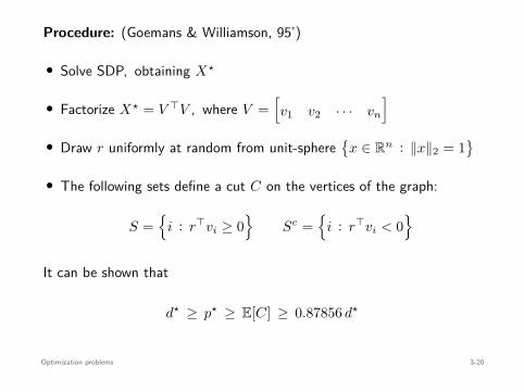
Solving Optimization Problems
CVX & other solvers are great for
• prototyping
• small-scale problems
Large-scale problems & real-time solutions require tailored solvers
Optimization problems 3-21
Solving Optimization Problems
CVX & other solvers are great for
• prototyping
• small-scale problems
Large-scale problems & real-time solutions require tailored solvers
Optimization problems 3-21
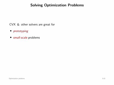
Solving Optimization Problems
CVX & other solvers are great for
• prototyping
• small-scale problems
Large-scale problems & real-time solutions require tailored solvers
Optimization problems 3-21
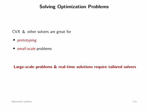
Solving Optimization Problems
CVX & other solvers are great for
• prototyping
• small-scale problems
Large-scale problems & real-time solutions require tailored solvers
Optimization problems 3-21

Example:
minimizex
∥x∥1
subject to Ax = b
where A ∈ Rm×n and b ∈ Rm are generated randomly.
For n = 5000 and m = 500,
• CVX: 56.16 s
• SPGL1: 0.82 s (tailored solver)
Optimization problems 3-22
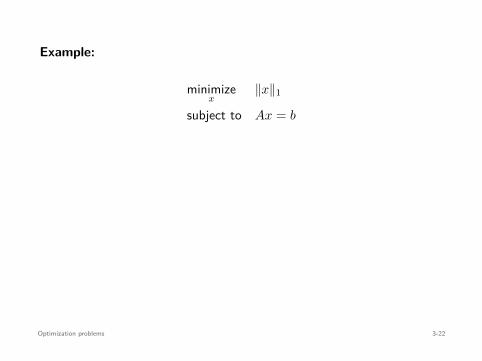
Example:
minimizex
∥x∥1
subject to Ax = b
where A ∈ Rm×n and b ∈ Rm are generated randomly.
For n = 5000 and m = 500,
• CVX: 56.16 s
• SPGL1: 0.82 s (tailored solver)
Optimization problems 3-22
Example:
minimizex
∥x∥1
subject to Ax = b
where A ∈ Rm×n and b ∈ Rm are generated randomly.
For n = 5000 and m = 500,
• CVX: 56.16 s
• SPGL1: 0.82 s (tailored solver)
Optimization problems 3-22
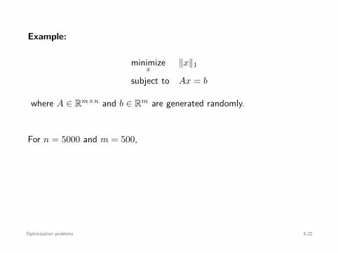
Example:
minimizex
∥x∥1
subject to Ax = b
where A ∈ Rm×n and b ∈ Rm are generated randomly.
For n = 5000 and m = 500,
• CVX: 56.16 s
• SPGL1: 0.82 s (tailored solver)
Optimization problems 3-22
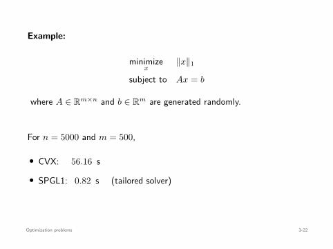
Example:
minimizex
∥x∥1
subject to Ax = b
where A ∈ Rm×n and b ∈ Rm are generated randomly.
For n = 5000 and m = 500,
• CVX: 56.16 s
• SPGL1: 0.82 s (tailored solver)
Optimization problems 3-22
Optimization Algorithms
• Unconstrained & differentiable
Gradient descent (and Nesterov’s acceleration scheme)Block coordinate descentNewton (and approximations)
• Constrained & differentiable
Projection methods (projected gradient descent, Frank-Wolfe, . . . )Interior-point algorithms (classes LP, QP, SOCP, SDP)
• Non-differentiable
Subgradient descentProximal methods (proximal gradient descent, ADMM, primal-dual)
And now, neural networks!
Optimization problems 3-23
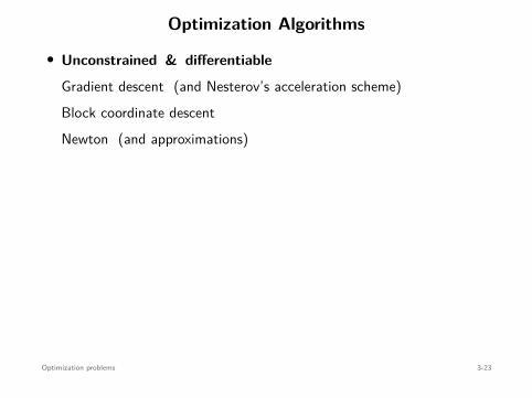
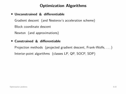
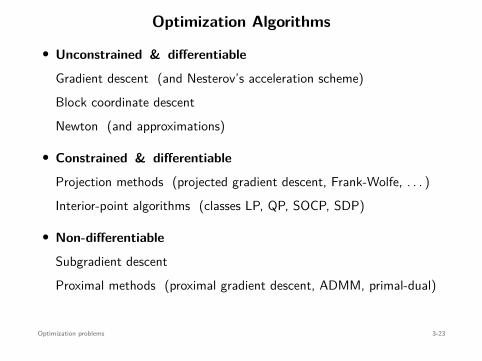
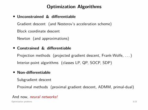
Optimization Algorithms
• Unconstrained & differentiable
Gradient descent (and Nesterov’s acceleration scheme)Block coordinate descentNewton (and approximations)
• Constrained & differentiable
Projection methods (projected gradient descent, Frank-Wolfe, . . . )Interior-point algorithms (classes LP, QP, SOCP, SDP)
• Non-differentiable
Subgradient descentProximal methods (proximal gradient descent, ADMM, primal-dual)
And now, neural networks!Optimization problems 3-23

Nesterov’s acceleration scheme
minimizex
f(x)
• f : Rn → R : differentiable
• ∇f : Lipschitz-continuous, i.e., there exists L ≥ 0 such that
∥∇f(y) − ∇f(x)∥2 ≤ L∥y − x∥2 , for all x, y ∈ dom f
• f⋆ := minx f(x) > −∞
Optimization problems 3-24
Nesterov’s acceleration scheme
minimizex
f(x)
• f : Rn → R : differentiable
• ∇f : Lipschitz-continuous, i.e., there exists L ≥ 0 such that
∥∇f(y) − ∇f(x)∥2 ≤ L∥y − x∥2 , for all x, y ∈ dom f
• f⋆ := minx f(x) > −∞
Optimization problems 3-24
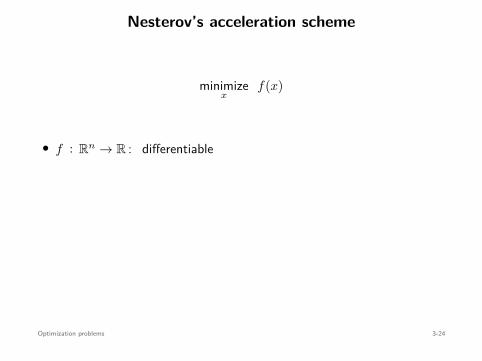
Nesterov’s acceleration scheme
minimizex
f(x)
• f : Rn → R : differentiable
• ∇f : Lipschitz-continuous, i.e., there exists L ≥ 0 such that
∥∇f(y) − ∇f(x)∥2 ≤ L∥y − x∥2 , for all x, y ∈ dom f
• f⋆ := minx f(x) > −∞
Optimization problems 3-24
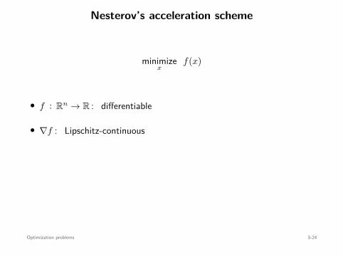
Nesterov’s acceleration scheme
minimizex
f(x)
• f : Rn → R : differentiable
• ∇f : Lipschitz-continuous
, i.e., there exists L ≥ 0 such that
∥∇f(y) − ∇f(x)∥2 ≤ L∥y − x∥2 , for all x, y ∈ dom f
• f⋆ := minx f(x) > −∞
Optimization problems 3-24
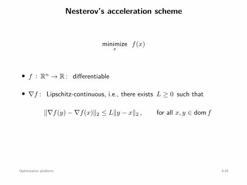
Nesterov’s acceleration scheme
minimizex
f(x)
• f : Rn → R : differentiable
• ∇f : Lipschitz-continuous, i.e., there exists L ≥ 0 such that
∥∇f(y) − ∇f(x)∥2 ≤ L∥y − x∥2 , for all x, y ∈ dom f
• f⋆ := minx f(x) > −∞
Optimization problems 3-24
Nesterov’s acceleration scheme
minimizex
f(x)
• f : Rn → R : differentiable
• ∇f : Lipschitz-continuous, i.e., there exists L ≥ 0 such that
∥∇f(y) − ∇f(x)∥2 ≤ L∥y − x∥2 , for all x, y ∈ dom f
• f⋆ := minx f(x) > −∞
Optimization problems 3-24

Nesterov’s acceleration scheme
Gradient descent:
starting at arbitrary x0 ∈ Rn,
xk+1 = xk − 1L
∇f(xk
)f(xk) − f⋆ ≤ L
2k
∥∥x0 − x⋆∥∥2
2
Nesterov’s method: starting at arbitrary y0 ∈ Rn,
xk+1 = yk − 1L
∇f(yk
)
yk+1 = xk − k − 1k + 2
(xk+1 − xk
) f(xk) − f⋆ ≤ 2L
(k + 1)2
∥∥x0 − x⋆∥∥2
2
Optimization problems 3-25
Nesterov’s acceleration scheme
Gradient descent: starting at arbitrary x0 ∈ Rn,
xk+1 = xk − 1L
∇f(xk
)
f(xk) − f⋆ ≤ L
2k
∥∥x0 − x⋆∥∥2
2
Nesterov’s method: starting at arbitrary y0 ∈ Rn,
xk+1 = yk − 1L
∇f(yk
)
yk+1 = xk − k − 1k + 2
(xk+1 − xk
) f(xk) − f⋆ ≤ 2L
(k + 1)2
∥∥x0 − x⋆∥∥2
2
Optimization problems 3-25
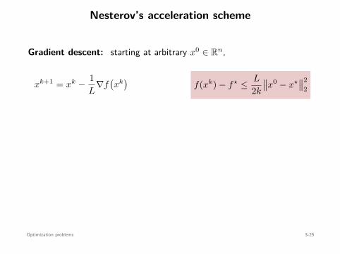
Nesterov’s acceleration scheme
Gradient descent: starting at arbitrary x0 ∈ Rn,
xk+1 = xk − 1L
∇f(xk
)f(xk) − f⋆ ≤ L
2k
∥∥x0 − x⋆∥∥2
2
Nesterov’s method: starting at arbitrary y0 ∈ Rn,
xk+1 = yk − 1L
∇f(yk
)
yk+1 = xk − k − 1k + 2
(xk+1 − xk
) f(xk) − f⋆ ≤ 2L
(k + 1)2
∥∥x0 − x⋆∥∥2
2
Optimization problems 3-25
Nesterov’s acceleration scheme
Gradient descent: starting at arbitrary x0 ∈ Rn,
xk+1 = xk − 1L
∇f(xk
)f(xk) − f⋆ ≤ L
2k
∥∥x0 − x⋆∥∥2
2
Nesterov’s method: starting at arbitrary y0 ∈ Rn,
xk+1 = yk − 1L
∇f(yk
)
yk+1 = xk − k − 1k + 2
(xk+1 − xk
) f(xk) − f⋆ ≤ 2L
(k + 1)2
∥∥x0 − x⋆∥∥2
2
Optimization problems 3-25
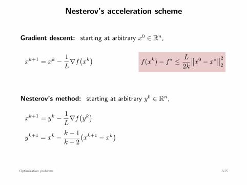
Nesterov’s acceleration scheme
Gradient descent: starting at arbitrary x0 ∈ Rn,
xk+1 = xk − 1L
∇f(xk
)f(xk) − f⋆ ≤ L
2k
∥∥x0 − x⋆∥∥2
2
Nesterov’s method: starting at arbitrary y0 ∈ Rn,
xk+1 = yk − 1L
∇f(yk
)
yk+1 = xk − k − 1k + 2
(xk+1 − xk
)
f(xk) − f⋆ ≤ 2L
(k + 1)2
∥∥x0 − x⋆∥∥2
2
Optimization problems 3-25
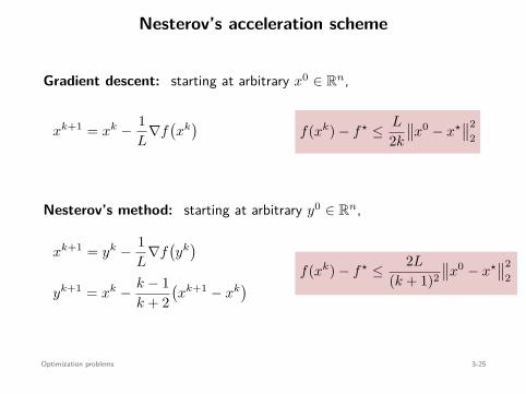
Nesterov’s acceleration scheme
Gradient descent: starting at arbitrary x0 ∈ Rn,
xk+1 = xk − 1L
∇f(xk
)f(xk) − f⋆ ≤ L
2k
∥∥x0 − x⋆∥∥2
2
Nesterov’s method: starting at arbitrary y0 ∈ Rn,
xk+1 = yk − 1L
∇f(yk
)
yk+1 = xk − k − 1k + 2
(xk+1 − xk
) f(xk) − f⋆ ≤ 2L
(k + 1)2
∥∥x0 − x⋆∥∥2
2
Optimization problems 3-25
Example
minimizex∈Rn
logm∑
i=1exp
(a⊤
i x + b)
randomly generated data with m = 500, n = 50
iterations k
|f(xk) − f⋆|/|f⋆|
gradient descent
Nesterov
Optimization problems 3-26
Example
minimizex∈Rn
logm∑
i=1exp
(a⊤
i x + b)
randomly generated data with m = 500, n = 50
iterations k
|f(xk) − f⋆|/|f⋆|
gradient descent
Nesterov
Optimization problems 3-26
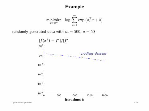
Example
minimizex∈Rn
logm∑
i=1exp
(a⊤
i x + b)
randomly generated data with m = 500, n = 50
iterations k
|f(xk) − f⋆|/|f⋆|
gradient descent
Nesterov
Optimization problems 3-26
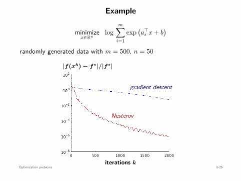
Example
minimizex∈Rn
logm∑
i=1exp
(a⊤
i x + b)
randomly generated data with m = 500, n = 50
iterations k
|f(xk) − f⋆|/|f⋆|
gradient descent
Nesterov
Optimization problems 3-26
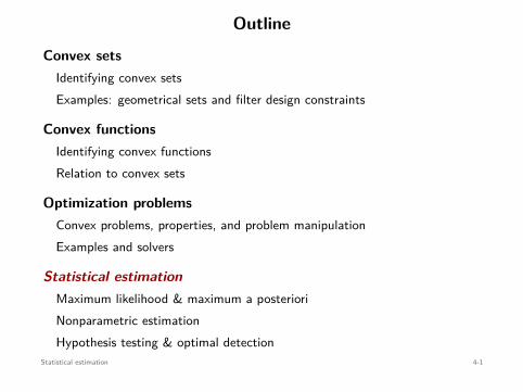
Outline
Convex setsIdentifying convex setsExamples: geometrical sets and filter design constraints
Convex functionsIdentifying convex functionsRelation to convex sets
Optimization problemsConvex problems, properties, and problem manipulationExamples and solvers
Statistical estimationMaximum likelihood & maximum a posterioriNonparametric estimationHypothesis testing & optimal detection
Statistical estimation 4-1

Maximum likelihood
Y ∈ Rm: random vector with density fY
(y ; x
)
x ∈ Rn: parameter to estimate (we may know that x ∈ C ⊂ Rn)
Maximum Likelihood (ML) estimate: Given realization y of Y ,
maximizex
fY
(y ; x
)
subject to x ∈ C
⇐⇒ maximizex
log fY
(y ; x
)
subject to x ∈ C
⇐⇒ minimizex
− log fY
(y ; x
)
subject to x ∈ C
negative log-likelihood
Statistical estimation 4-2
Maximum likelihood
Y ∈ Rm: random vector with density fY
(y ; x
)
x ∈ Rn: parameter to estimate
(we may know that x ∈ C ⊂ Rn)
Maximum Likelihood (ML) estimate: Given realization y of Y ,
maximizex
fY
(y ; x
)
subject to x ∈ C
⇐⇒ maximizex
log fY
(y ; x
)
subject to x ∈ C
⇐⇒ minimizex
− log fY
(y ; x
)
subject to x ∈ C
negative log-likelihood
Statistical estimation 4-2
Maximum likelihood
Y ∈ Rm: random vector with density fY
(y ; x
)
x ∈ Rn: parameter to estimate (we may know that x ∈ C ⊂ Rn)
Maximum Likelihood (ML) estimate: Given realization y of Y ,
maximizex
fY
(y ; x
)
subject to x ∈ C
⇐⇒ maximizex
log fY
(y ; x
)
subject to x ∈ C
⇐⇒ minimizex
− log fY
(y ; x
)
subject to x ∈ C
negative log-likelihood
Statistical estimation 4-2
Maximum likelihood
Y ∈ Rm: random vector with density fY
(y ; x
)
x ∈ Rn: parameter to estimate (we may know that x ∈ C ⊂ Rn)
Maximum Likelihood (ML) estimate: Given realization y of Y ,
maximizex
fY
(y ; x
)
subject to x ∈ C
⇐⇒ maximizex
log fY
(y ; x
)
subject to x ∈ C
⇐⇒ minimizex
− log fY
(y ; x
)
subject to x ∈ C
negative log-likelihood
Statistical estimation 4-2
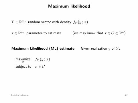
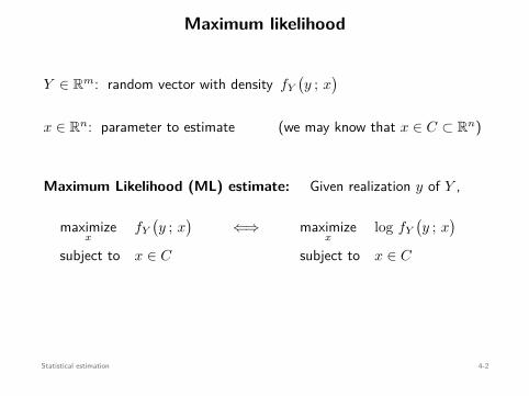
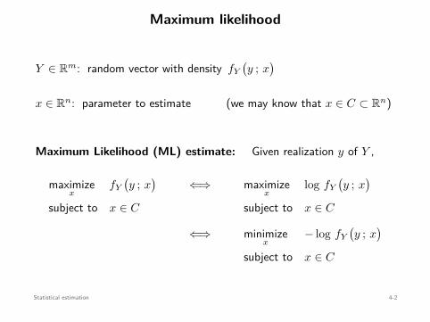
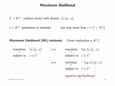
Maximum likelihood
Y ∈ Rm: random vector with density fY
(y ; x
)
x ∈ Rn: parameter to estimate (we may know that x ∈ C ⊂ Rn)
Maximum Likelihood (ML) estimate: Given realization y of Y ,
maximizex
fY
(y ; x
)
subject to x ∈ C
⇐⇒ maximizex
log fY
(y ; x
)
subject to x ∈ C
⇐⇒ minimizex
− log fY
(y ; x
)
subject to x ∈ C
negative log-likelihoodStatistical estimation 4-2
Maximum likelihoodExample: linear measurement model
• Parameter to estimate: x ∈ Rn
• Observations: Yi = a⊤i x + Vi, i = 1, . . . , m, for known ai ∈ Rn
Vi: iid copies of random variable V with density fV (v)
=⇒ Yi has density fV (yi − a⊤i x) and Yi’s are independent
=⇒ fY1···Ym(y1, . . . , ym) =m∏
i=1fYi(yi) =
m∏
i=1fV (yi − a⊤
i x)
The ai’s will denote the rows of A =
— a⊤1 —...
— a⊤m —
∈ Rm×n
Statistical estimation 4-3
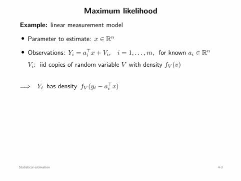
Maximum likelihoodExample: linear measurement model
• Parameter to estimate: x ∈ Rn
• Observations: Yi = a⊤i x + Vi, i = 1, . . . , m, for known ai ∈ Rn
Vi: iid copies of random variable V with density fV (v)
=⇒ Yi has density fV (yi − a⊤i x)
and Yi’s are independent
=⇒ fY1···Ym(y1, . . . , ym) =m∏
i=1fYi(yi) =
m∏
i=1fV (yi − a⊤
i x)
The ai’s will denote the rows of A =
— a⊤1 —...
— a⊤m —
∈ Rm×n
Statistical estimation 4-3
Maximum likelihoodExample: linear measurement model
• Parameter to estimate: x ∈ Rn
• Observations: Yi = a⊤i x + Vi, i = 1, . . . , m, for known ai ∈ Rn
Vi: iid copies of random variable V with density fV (v)
=⇒ Yi has density fV (yi − a⊤i x) and Yi’s are independent
=⇒ fY1···Ym(y1, . . . , ym) =m∏
i=1fYi(yi) =
m∏
i=1fV (yi − a⊤
i x)
The ai’s will denote the rows of A =
— a⊤1 —...
— a⊤m —
∈ Rm×n
Statistical estimation 4-3
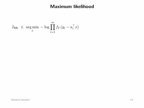
Maximum likelihood
xML ∈ arg minx
− logm∏
i=1fV (yi − a⊤
i x)
= arg minx
−m∑
i=1log fV (yi − a⊤
i x)
Common noise densities:
Gaussian: V ∼ N (0, σ2) fV (v) = 1√2πσ2 exp
(− v2
2σ2
)
xML ∈ arg minx
−m∑
i=1log 1√
2πσ2exp
(− (yi − a⊤
i x)2
2σ2
)
= arg minx
12σ2
m∑
i=1
(yi − a⊤
i x)2
= arg minx
12σ2
∥∥y − Ax∥∥2
2 Convex
Statistical estimation 4-4
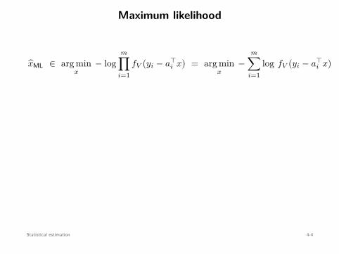
Maximum likelihood
xML ∈ arg minx
− logm∏
i=1fV (yi − a⊤
i x) = arg minx
−m∑
i=1log fV (yi − a⊤
i x)
Common noise densities:
Gaussian: V ∼ N (0, σ2) fV (v) = 1√2πσ2 exp
(− v2
2σ2
)
xML ∈ arg minx
−m∑
i=1log 1√
2πσ2exp
(− (yi − a⊤
i x)2
2σ2
)
= arg minx
12σ2
m∑
i=1
(yi − a⊤
i x)2
= arg minx
12σ2
∥∥y − Ax∥∥2
2 Convex
Statistical estimation 4-4
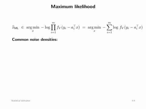
Maximum likelihood
xML ∈ arg minx
− logm∏
i=1fV (yi − a⊤
i x) = arg minx
−m∑
i=1log fV (yi − a⊤
i x)
Common noise densities:
Gaussian: V ∼ N (0, σ2) fV (v) = 1√2πσ2 exp
(− v2
2σ2
)
xML ∈ arg minx
−m∑
i=1log 1√
2πσ2exp
(− (yi − a⊤
i x)2
2σ2
)
= arg minx
12σ2
m∑
i=1
(yi − a⊤
i x)2
= arg minx
12σ2
∥∥y − Ax∥∥2
2 Convex
Statistical estimation 4-4
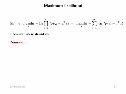
Maximum likelihood
xML ∈ arg minx
− logm∏
i=1fV (yi − a⊤
i x) = arg minx
−m∑
i=1log fV (yi − a⊤
i x)
Common noise densities:
Gaussian:
V ∼ N (0, σ2) fV (v) = 1√2πσ2 exp
(− v2
2σ2
)
xML ∈ arg minx
−m∑
i=1log 1√
2πσ2exp
(− (yi − a⊤
i x)2
2σ2
)
= arg minx
12σ2
m∑
i=1
(yi − a⊤
i x)2
= arg minx
12σ2
∥∥y − Ax∥∥2
2 Convex
Statistical estimation 4-4
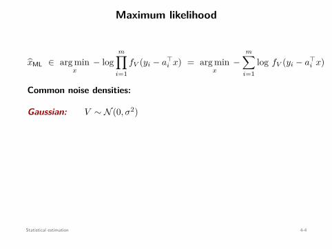
Maximum likelihood
xML ∈ arg minx
− logm∏
i=1fV (yi − a⊤
i x) = arg minx
−m∑
i=1log fV (yi − a⊤
i x)
Common noise densities:
Gaussian: V ∼ N (0, σ2)
fV (v) = 1√2πσ2 exp
(− v2
2σ2
)
xML ∈ arg minx
−m∑
i=1log 1√
2πσ2exp
(− (yi − a⊤
i x)2
2σ2
)
= arg minx
12σ2
m∑
i=1
(yi − a⊤
i x)2
= arg minx
12σ2
∥∥y − Ax∥∥2
2 Convex
Statistical estimation 4-4
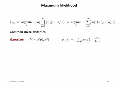
Maximum likelihood
xML ∈ arg minx
− logm∏
i=1fV (yi − a⊤
i x) = arg minx
−m∑
i=1log fV (yi − a⊤
i x)
Common noise densities:
Gaussian: V ∼ N (0, σ2) fV (v) = 1√2πσ2 exp
(− v2
2σ2
)
xML ∈ arg minx
−m∑
i=1log 1√
2πσ2exp
(− (yi − a⊤
i x)2
2σ2
)
= arg minx
12σ2
m∑
i=1
(yi − a⊤
i x)2
= arg minx
12σ2
∥∥y − Ax∥∥2
2 Convex
Statistical estimation 4-4
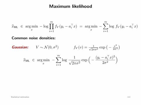
Maximum likelihood
xML ∈ arg minx
− logm∏
i=1fV (yi − a⊤
i x) = arg minx
−m∑
i=1log fV (yi − a⊤
i x)
Common noise densities:
Gaussian: V ∼ N (0, σ2) fV (v) = 1√2πσ2 exp
(− v2
2σ2
)
xML ∈ arg minx
−m∑
i=1log 1√
2πσ2exp
(− (yi − a⊤
i x)2
2σ2
)
= arg minx
12σ2
m∑
i=1
(yi − a⊤
i x)2
= arg minx
12σ2
∥∥y − Ax∥∥2
2 Convex
Statistical estimation 4-4
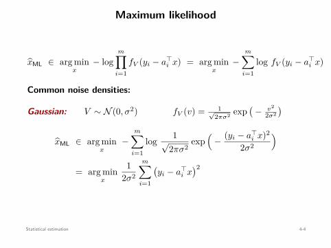
Maximum likelihood
xML ∈ arg minx
− logm∏
i=1fV (yi − a⊤
i x) = arg minx
−m∑
i=1log fV (yi − a⊤
i x)
Common noise densities:
Gaussian: V ∼ N (0, σ2) fV (v) = 1√2πσ2 exp
(− v2
2σ2
)
xML ∈ arg minx
−m∑
i=1log 1√
2πσ2exp
(− (yi − a⊤
i x)2
2σ2
)
= arg minx
12σ2
m∑
i=1
(yi − a⊤
i x)2
= arg minx
12σ2
∥∥y − Ax∥∥2
2 Convex
Statistical estimation 4-4
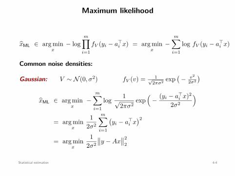
Maximum likelihood
xML ∈ arg minx
− logm∏
i=1fV (yi − a⊤
i x) = arg minx
−m∑
i=1log fV (yi − a⊤
i x)
Common noise densities:
Gaussian: V ∼ N (0, σ2) fV (v) = 1√2πσ2 exp
(− v2
2σ2
)
xML ∈ arg minx
−m∑
i=1log 1√
2πσ2exp
(− (yi − a⊤
i x)2
2σ2
)
= arg minx
12σ2
m∑
i=1
(yi − a⊤
i x)2
= arg minx
12σ2
∥∥y − Ax∥∥2
2
Convex
Statistical estimation 4-4
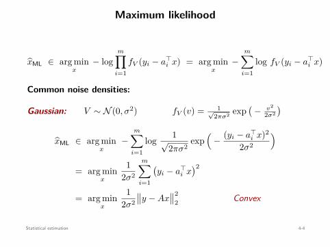
Maximum likelihood
xML ∈ arg minx
− logm∏
i=1fV (yi − a⊤
i x) = arg minx
−m∑
i=1log fV (yi − a⊤
i x)
Common noise densities:
Gaussian: V ∼ N (0, σ2) fV (v) = 1√2πσ2 exp
(− v2
2σ2
)
xML ∈ arg minx
−m∑
i=1log 1√
2πσ2exp
(− (yi − a⊤
i x)2
2σ2
)
= arg minx
12σ2
m∑
i=1
(yi − a⊤
i x)2
= arg minx
12σ2
∥∥y − Ax∥∥2
2 Convex
Statistical estimation 4-4
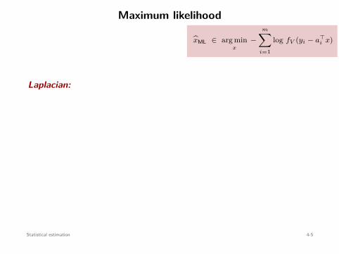
Maximum likelihood
xML ∈ arg minx
−m∑
i=1
log fV (yi − a⊤i x)
Laplacian:
V ∼ L(0, a) fV (v) = 1√2a
exp(
− |v|a
)(a > 0)
xML ∈ arg minx
−m∑
i=1log 1√
2aexp
(− |yi − a⊤
i x|a
)
= arg minx
1a
m∑
i=1
∣∣yi − a⊤i x
∣∣
= arg minx
1a
∥∥y − Ax∥∥
1 Convex
Statistical estimation 4-5
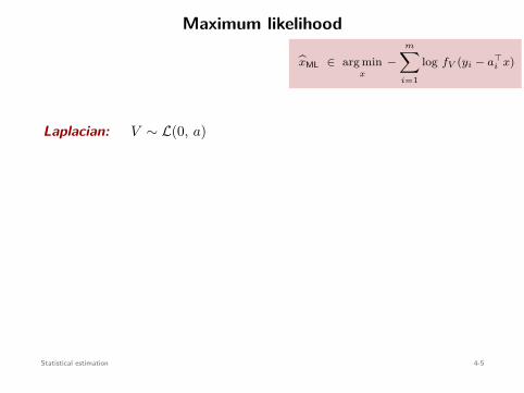
Maximum likelihood
xML ∈ arg minx
−m∑
i=1
log fV (yi − a⊤i x)
Laplacian: V ∼ L(0, a)
fV (v) = 1√2a
exp(
− |v|a
)(a > 0)
xML ∈ arg minx
−m∑
i=1log 1√
2aexp
(− |yi − a⊤
i x|a
)
= arg minx
1a
m∑
i=1
∣∣yi − a⊤i x
∣∣
= arg minx
1a
∥∥y − Ax∥∥
1 Convex
Statistical estimation 4-5
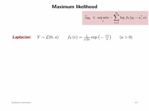
Maximum likelihood
xML ∈ arg minx
−m∑
i=1
log fV (yi − a⊤i x)
Laplacian: V ∼ L(0, a) fV (v) = 1√2a
exp(
− |v|a
)(a > 0)
xML ∈ arg minx
−m∑
i=1log 1√
2aexp
(− |yi − a⊤
i x|a
)
= arg minx
1a
m∑
i=1
∣∣yi − a⊤i x
∣∣
= arg minx
1a
∥∥y − Ax∥∥
1 Convex
Statistical estimation 4-5
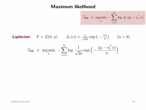
Maximum likelihood
xML ∈ arg minx
−m∑
i=1
log fV (yi − a⊤i x)
Laplacian: V ∼ L(0, a) fV (v) = 1√2a
exp(
− |v|a
)(a > 0)
xML ∈ arg minx
−m∑
i=1log 1√
2aexp
(− |yi − a⊤
i x|a
)
= arg minx
1a
m∑
i=1
∣∣yi − a⊤i x
∣∣
= arg minx
1a
∥∥y − Ax∥∥
1 Convex
Statistical estimation 4-5
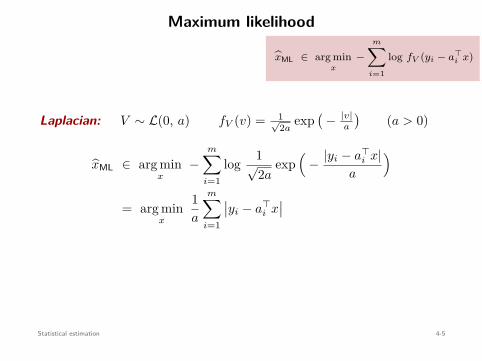
Maximum likelihood
xML ∈ arg minx
−m∑
i=1
log fV (yi − a⊤i x)
Laplacian: V ∼ L(0, a) fV (v) = 1√2a
exp(
− |v|a
)(a > 0)
xML ∈ arg minx
−m∑
i=1log 1√
2aexp
(− |yi − a⊤
i x|a
)
= arg minx
1a
m∑
i=1
∣∣yi − a⊤i x
∣∣
= arg minx
1a
∥∥y − Ax∥∥
1 Convex
Statistical estimation 4-5
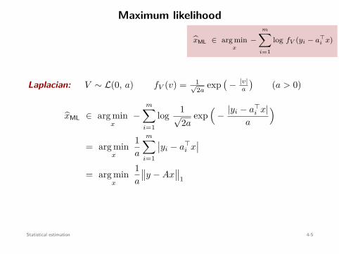
Maximum likelihood
xML ∈ arg minx
−m∑
i=1
log fV (yi − a⊤i x)
Laplacian: V ∼ L(0, a) fV (v) = 1√2a
exp(
− |v|a
)(a > 0)
xML ∈ arg minx
−m∑
i=1log 1√
2aexp
(− |yi − a⊤
i x|a
)
= arg minx
1a
m∑
i=1
∣∣yi − a⊤i x
∣∣
= arg minx
1a
∥∥y − Ax∥∥
1
Convex
Statistical estimation 4-5
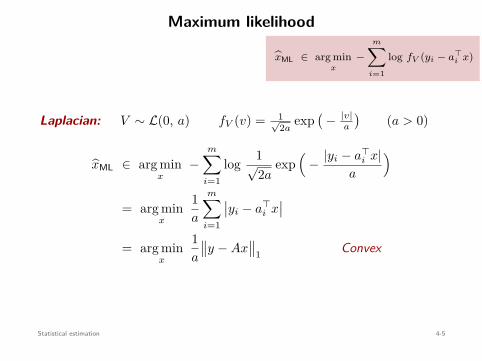
Maximum likelihood
xML ∈ arg minx
−m∑
i=1
log fV (yi − a⊤i x)
Laplacian: V ∼ L(0, a) fV (v) = 1√2a
exp(
− |v|a
)(a > 0)
xML ∈ arg minx
−m∑
i=1log 1√
2aexp
(− |yi − a⊤
i x|a
)
= arg minx
1a
m∑
i=1
∣∣yi − a⊤i x
∣∣
= arg minx
1a
∥∥y − Ax∥∥
1 Convex
Statistical estimation 4-5

Maximum likelihood
Uniform:
V ∼ U(−c, c) fV (v) = 1
2c , |v| ≤ c
0 , oth.
xML ∈ arg minx
−m∑
i=1log fV (yi − a⊤
i x)
= arg minx
− ∑mi=1 log 1
2c
s.t. |yi − a⊤i x| ≤ c , i = 1, . . . , m .
= find x
s.t. ∥y − Ax∥∞ ≤ c
feasibility problem (convex)
Statistical estimation 4-6
Maximum likelihood
Uniform: V ∼ U(−c, c)
fV (v) = 1
2c , |v| ≤ c
0 , oth.
xML ∈ arg minx
−m∑
i=1log fV (yi − a⊤
i x)
= arg minx
− ∑mi=1 log 1
2c
s.t. |yi − a⊤i x| ≤ c , i = 1, . . . , m .
= find x
s.t. ∥y − Ax∥∞ ≤ c
feasibility problem (convex)
Statistical estimation 4-6
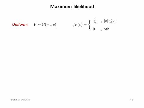
Maximum likelihood
Uniform: V ∼ U(−c, c) fV (v) = 1
2c , |v| ≤ c
0 , oth.
xML ∈ arg minx
−m∑
i=1log fV (yi − a⊤
i x)
= arg minx
− ∑mi=1 log 1
2c
s.t. |yi − a⊤i x| ≤ c , i = 1, . . . , m .
= find x
s.t. ∥y − Ax∥∞ ≤ c
feasibility problem (convex)
Statistical estimation 4-6
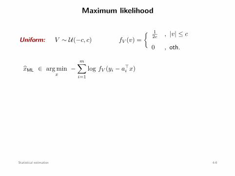
Maximum likelihood
Uniform: V ∼ U(−c, c) fV (v) = 1
2c , |v| ≤ c
0 , oth.
xML ∈ arg minx
−m∑
i=1log fV (yi − a⊤
i x)
= arg minx
− ∑mi=1 log 1
2c
s.t. |yi − a⊤i x| ≤ c , i = 1, . . . , m .
= find x
s.t. ∥y − Ax∥∞ ≤ c
feasibility problem (convex)
Statistical estimation 4-6
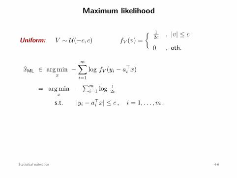
Maximum likelihood
Uniform: V ∼ U(−c, c) fV (v) = 1
2c , |v| ≤ c
0 , oth.
xML ∈ arg minx
−m∑
i=1log fV (yi − a⊤
i x)
= arg minx
− ∑mi=1 log 1
2c
s.t. |yi − a⊤i x| ≤ c , i = 1, . . . , m .
= find x
s.t. ∥y − Ax∥∞ ≤ c
feasibility problem (convex)
Statistical estimation 4-6
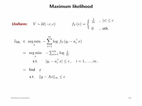
Maximum likelihood
Uniform: V ∼ U(−c, c) fV (v) = 1
2c , |v| ≤ c
0 , oth.
xML ∈ arg minx
−m∑
i=1log fV (yi − a⊤
i x)
= arg minx
− ∑mi=1 log 1
2c
s.t. |yi − a⊤i x| ≤ c , i = 1, . . . , m .
= find x
s.t. ∥y − Ax∥∞ ≤ c
feasibility problem (convex)
Statistical estimation 4-6
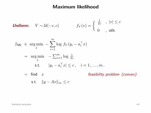
Maximum likelihood
Uniform: V ∼ U(−c, c) fV (v) = 1
2c , |v| ≤ c
0 , oth.
xML ∈ arg minx
−m∑
i=1log fV (yi − a⊤
i x)
= arg minx
− ∑mi=1 log 1
2c
s.t. |yi − a⊤i x| ≤ c , i = 1, . . . , m .
= find x
s.t. ∥y − Ax∥∞ ≤ c
feasibility problem (convex)
Statistical estimation 4-6

Example with a discrete RV
Y ∈ N: # of traffic accidents in a given period
Y ∼ Poisson(µ) P(Y = k) = e−µµk
k ! , k = 0, 1, . . .
Assumption: µ depends on vector of explanatory variables U ∈ Rn as
µ = a⊤U + b , a ∈ Rn , b ∈ R
e.g., U1 = traffic flow during the period, U2 = rainfall, . . .
Goal:
Given m independent observations(
U (i), Y (i))m
i=1, estimate a and b.
Statistical estimation 4-7
Example with a discrete RV
Y ∈ N: # of traffic accidents in a given period
Y ∼ Poisson(µ)
P(Y = k) = e−µµk
k ! , k = 0, 1, . . .
Assumption: µ depends on vector of explanatory variables U ∈ Rn as
µ = a⊤U + b , a ∈ Rn , b ∈ R
e.g., U1 = traffic flow during the period, U2 = rainfall, . . .
Goal:
Given m independent observations(
U (i), Y (i))m
i=1, estimate a and b.
Statistical estimation 4-7
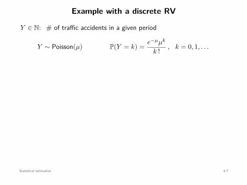
Example with a discrete RV
Y ∈ N: # of traffic accidents in a given period
Y ∼ Poisson(µ) P(Y = k) = e−µµk
k ! , k = 0, 1, . . .
Assumption: µ depends on vector of explanatory variables U ∈ Rn as
µ = a⊤U + b , a ∈ Rn , b ∈ R
e.g., U1 = traffic flow during the period, U2 = rainfall, . . .
Goal:
Given m independent observations(
U (i), Y (i))m
i=1, estimate a and b.
Statistical estimation 4-7
Example with a discrete RV
Y ∈ N: # of traffic accidents in a given period
Y ∼ Poisson(µ) P(Y = k) = e−µµk
k ! , k = 0, 1, . . .
Assumption: µ depends on vector of explanatory variables U ∈ Rn as
µ = a⊤U + b , a ∈ Rn , b ∈ R
e.g., U1 = traffic flow during the period, U2 = rainfall, . . .
Goal:
Given m independent observations(
U (i), Y (i))m
i=1, estimate a and b.
Statistical estimation 4-7
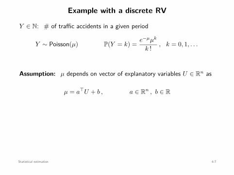
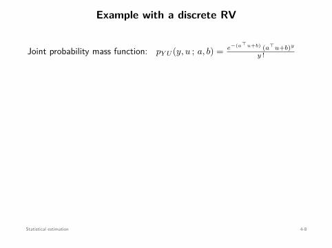
Example with a discrete RV
Joint probability mass function: pY U (y, u ; a, b) = e−(a⊤u+b) (a⊤u+b)y
y !
ML estimator:
(aML, bML
)∈ arg min
a,b−
m∑
i=1log pY U (yi, ui ; a, b)
= arg mina,b
−m∑
i=1log e−(a⊤u(i)+b) (a⊤u(i) + b)y(i)
y(i) !
= arg mina,b
m∑
i=1a⊤u(i) + b
︸ ︷︷ ︸affine
− y(i) log(a⊤u(i) + b
)
︸ ︷︷ ︸convex
Convex
Statistical estimation 4-8
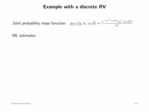
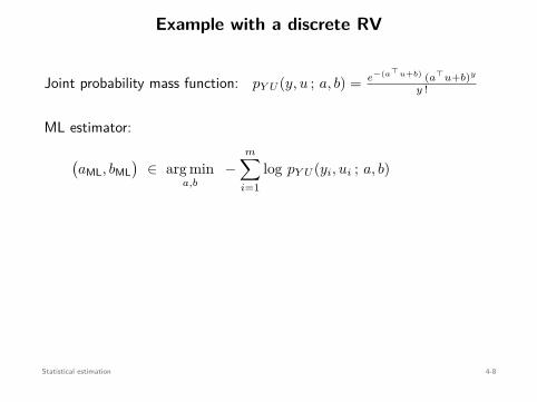
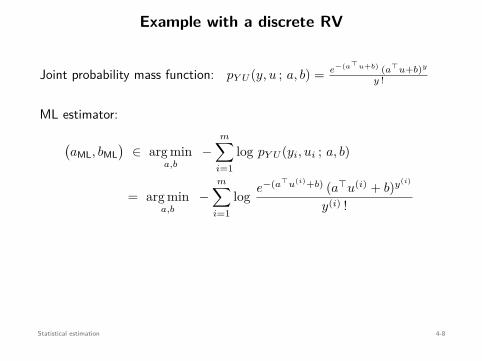
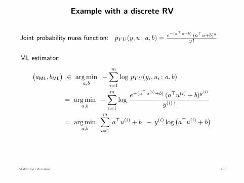
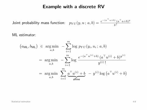
Example with a discrete RV
Joint probability mass function: pY U (y, u ; a, b) = e−(a⊤u+b) (a⊤u+b)y
y !
ML estimator:
(aML, bML
)∈ arg min
a,b−
m∑
i=1log pY U (yi, ui ; a, b)
= arg mina,b
−m∑
i=1log e−(a⊤u(i)+b) (a⊤u(i) + b)y(i)
y(i) !
= arg mina,b
m∑
i=1a⊤u(i) + b︸ ︷︷ ︸
affine
− y(i) log(a⊤u(i) + b
)
︸ ︷︷ ︸convex
Convex
Statistical estimation 4-8
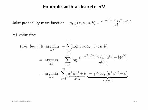
Example with a discrete RV
Joint probability mass function: pY U (y, u ; a, b) = e−(a⊤u+b) (a⊤u+b)y
y !
ML estimator:
(aML, bML
)∈ arg min
a,b−
m∑
i=1log pY U (yi, ui ; a, b)
= arg mina,b
−m∑
i=1log e−(a⊤u(i)+b) (a⊤u(i) + b)y(i)
y(i) !
= arg mina,b
m∑
i=1a⊤u(i) + b︸ ︷︷ ︸
affine
− y(i) log(a⊤u(i) + b
)︸ ︷︷ ︸
convex
Convex
Statistical estimation 4-8
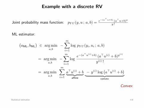
Example with a discrete RV
Joint probability mass function: pY U (y, u ; a, b) = e−(a⊤u+b) (a⊤u+b)y
y !
ML estimator:
(aML, bML
)∈ arg min
a,b−
m∑
i=1log pY U (yi, ui ; a, b)
= arg mina,b
−m∑
i=1log e−(a⊤u(i)+b) (a⊤u(i) + b)y(i)
y(i) !
= arg mina,b
m∑
i=1a⊤u(i) + b︸ ︷︷ ︸
affine
− y(i) log(a⊤u(i) + b
)︸ ︷︷ ︸
convex
Convex
Statistical estimation 4-8

Maximum a posteriori (MAP)
Y ∈ Rm: random vector w/ density fY (y)
X ∈ Rn: random vector to estimate no longer a parameterprior knowledge: fX(x)
MAP estimator:
xMAP ∈ arg maxx
fX|Y (x|y) Bayes= arg maxx
fY |X(y|x)fX(x)fY (y)
= arg maxx
fY |X(y|x)fX(x)
= arg maxx
log(fY |X(y|x)fX(x)
)
= arg minx
− log fY |X(y|x) − log fX(x)
Statistical estimation 4-9
Maximum a posteriori (MAP)
Y ∈ Rm: random vector w/ density fY (y)
X ∈ Rn: random vector to estimate
no longer a parameterprior knowledge: fX(x)
MAP estimator:
xMAP ∈ arg maxx
fX|Y (x|y) Bayes= arg maxx
fY |X(y|x)fX(x)fY (y)
= arg maxx
fY |X(y|x)fX(x)
= arg maxx
log(fY |X(y|x)fX(x)
)
= arg minx
− log fY |X(y|x) − log fX(x)
Statistical estimation 4-9
Maximum a posteriori (MAP)
Y ∈ Rm: random vector w/ density fY (y)
X ∈ Rn: random vector to estimate no longer a parameter
prior knowledge: fX(x)
MAP estimator:
xMAP ∈ arg maxx
fX|Y (x|y) Bayes= arg maxx
fY |X(y|x)fX(x)fY (y)
= arg maxx
fY |X(y|x)fX(x)
= arg maxx
log(fY |X(y|x)fX(x)
)
= arg minx
− log fY |X(y|x) − log fX(x)
Statistical estimation 4-9
Maximum a posteriori (MAP)
Y ∈ Rm: random vector w/ density fY (y)
X ∈ Rn: random vector to estimate no longer a parameterprior knowledge: fX(x)
MAP estimator:
xMAP ∈ arg maxx
fX|Y (x|y) Bayes= arg maxx
fY |X(y|x)fX(x)fY (y)
= arg maxx
fY |X(y|x)fX(x)
= arg maxx
log(fY |X(y|x)fX(x)
)
= arg minx
− log fY |X(y|x) − log fX(x)
Statistical estimation 4-9
Maximum a posteriori (MAP)
Y ∈ Rm: random vector w/ density fY (y)
X ∈ Rn: random vector to estimate no longer a parameterprior knowledge: fX(x)
MAP estimator:
xMAP ∈ arg maxx
fX|Y (x|y) Bayes= arg maxx
fY |X(y|x)fX(x)fY (y)
= arg maxx
fY |X(y|x)fX(x)
= arg maxx
log(fY |X(y|x)fX(x)
)
= arg minx
− log fY |X(y|x) − log fX(x)
Statistical estimation 4-9
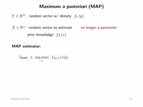
Maximum a posteriori (MAP)
Y ∈ Rm: random vector w/ density fY (y)
X ∈ Rn: random vector to estimate no longer a parameterprior knowledge: fX(x)
MAP estimator:
xMAP ∈ arg maxx
fX|Y (x|y)
Bayes= arg maxx
fY |X(y|x)fX(x)fY (y)
= arg maxx
fY |X(y|x)fX(x)
= arg maxx
log(fY |X(y|x)fX(x)
)
= arg minx
− log fY |X(y|x) − log fX(x)
Statistical estimation 4-9
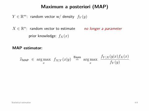
Maximum a posteriori (MAP)
Y ∈ Rm: random vector w/ density fY (y)
X ∈ Rn: random vector to estimate no longer a parameterprior knowledge: fX(x)
MAP estimator:
xMAP ∈ arg maxx
fX|Y (x|y) Bayes= arg maxx
fY |X(y|x)fX(x)fY (y)
= arg maxx
fY |X(y|x)fX(x)
= arg maxx
log(fY |X(y|x)fX(x)
)
= arg minx
− log fY |X(y|x) − log fX(x)
Statistical estimation 4-9
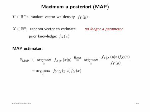
Maximum a posteriori (MAP)
Y ∈ Rm: random vector w/ density fY (y)
X ∈ Rn: random vector to estimate no longer a parameterprior knowledge: fX(x)
MAP estimator:
xMAP ∈ arg maxx
fX|Y (x|y) Bayes= arg maxx
fY |X(y|x)fX(x)fY (y)
= arg maxx
fY |X(y|x)fX(x)
= arg maxx
log(fY |X(y|x)fX(x)
)
= arg minx
− log fY |X(y|x) − log fX(x)
Statistical estimation 4-9
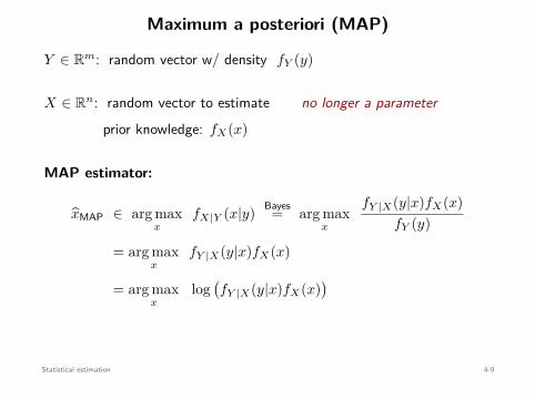
Maximum a posteriori (MAP)
Y ∈ Rm: random vector w/ density fY (y)
X ∈ Rn: random vector to estimate no longer a parameterprior knowledge: fX(x)
MAP estimator:
xMAP ∈ arg maxx
fX|Y (x|y) Bayes= arg maxx
fY |X(y|x)fX(x)fY (y)
= arg maxx
fY |X(y|x)fX(x)
= arg maxx
log(fY |X(y|x)fX(x)
)
= arg minx
− log fY |X(y|x) − log fX(x)
Statistical estimation 4-9
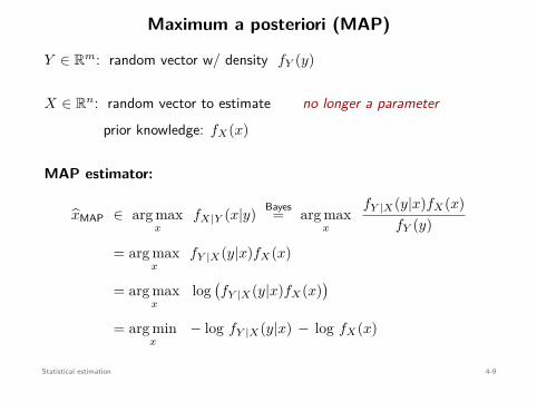
Maximum a posteriori (MAP)
Y ∈ Rm: random vector w/ density fY (y)
X ∈ Rn: random vector to estimate no longer a parameterprior knowledge: fX(x)
MAP estimator:
xMAP ∈ arg maxx
fX|Y (x|y) Bayes= arg maxx
fY |X(y|x)fX(x)fY (y)
= arg maxx
fY |X(y|x)fX(x)
= arg maxx
log(fY |X(y|x)fX(x)
)
= arg minx
− log fY |X(y|x) − log fX(x)
Statistical estimation 4-9
Maximum a posteriori (MAP)
Example: linear measurement model
• Observations: Yi = a⊤i X + Vi, i = 1, . . . , m , & Vi
iid= V ∼ U(−c, c)
fY1···Ym|X(y1, . . . , ym|x) =m∏
i=1fYi|X(yi|x) =
m∏
i=1U
(a⊤
i x − c , a⊤i x + c
)
• Random vector to estimate in Rn: X ∼ N(x, Σ
) (known x, Σ
)
fX(x) = 1(2π)n/2|Σ|1/2 exp
(− 1
2(x − x)⊤Σ−1(x − x))
xMAP ∈ arg minx
− log fY1···Ym|X(y1, . . . , ym|x) − log fX(x)
= arg minx
12 (x − x)⊤Σ−1(x − x)
s.t. ∥Ax − y∥∞ ≤ c
Convex
Statistical estimation 4-10
Maximum a posteriori (MAP)
Example: linear measurement model• Observations: Yi = a⊤
i X + Vi, i = 1, . . . , m
, & Viiid= V ∼ U(−c, c)
fY1···Ym|X(y1, . . . , ym|x) =m∏
i=1fYi|X(yi|x) =
m∏
i=1U
(a⊤
i x − c , a⊤i x + c
)
• Random vector to estimate in Rn: X ∼ N(x, Σ
) (known x, Σ
)
fX(x) = 1(2π)n/2|Σ|1/2 exp
(− 1
2(x − x)⊤Σ−1(x − x))
xMAP ∈ arg minx
− log fY1···Ym|X(y1, . . . , ym|x) − log fX(x)
= arg minx
12 (x − x)⊤Σ−1(x − x)
s.t. ∥Ax − y∥∞ ≤ c
Convex
Statistical estimation 4-10
Maximum a posteriori (MAP)
Example: linear measurement model• Observations: Yi = a⊤
i X + Vi, i = 1, . . . , m , & Viiid= V ∼ U(−c, c)
fY1···Ym|X(y1, . . . , ym|x)
=m∏
i=1fYi|X(yi|x) =
m∏
i=1U
(a⊤
i x − c , a⊤i x + c
)
• Random vector to estimate in Rn: X ∼ N(x, Σ
) (known x, Σ
)
fX(x) = 1(2π)n/2|Σ|1/2 exp
(− 1
2(x − x)⊤Σ−1(x − x))
xMAP ∈ arg minx
− log fY1···Ym|X(y1, . . . , ym|x) − log fX(x)
= arg minx
12 (x − x)⊤Σ−1(x − x)
s.t. ∥Ax − y∥∞ ≤ c
Convex
Statistical estimation 4-10
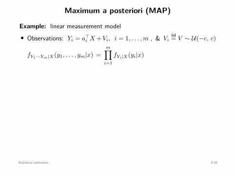
Maximum a posteriori (MAP)
Example: linear measurement model• Observations: Yi = a⊤
i X + Vi, i = 1, . . . , m , & Viiid= V ∼ U(−c, c)
fY1···Ym|X(y1, . . . , ym|x) =m∏
i=1fYi|X(yi|x)
=m∏
i=1U
(a⊤
i x − c , a⊤i x + c
)
• Random vector to estimate in Rn: X ∼ N(x, Σ
) (known x, Σ
)
fX(x) = 1(2π)n/2|Σ|1/2 exp
(− 1
2(x − x)⊤Σ−1(x − x))
xMAP ∈ arg minx
− log fY1···Ym|X(y1, . . . , ym|x) − log fX(x)
= arg minx
12 (x − x)⊤Σ−1(x − x)
s.t. ∥Ax − y∥∞ ≤ c
Convex
Statistical estimation 4-10
Maximum a posteriori (MAP)
Example: linear measurement model• Observations: Yi = a⊤
i X + Vi, i = 1, . . . , m , & Viiid= V ∼ U(−c, c)
fY1···Ym|X(y1, . . . , ym|x) =m∏
i=1fYi|X(yi|x) =
m∏
i=1U
(a⊤
i x − c , a⊤i x + c
)
• Random vector to estimate in Rn: X ∼ N(x, Σ
) (known x, Σ
)
fX(x) = 1(2π)n/2|Σ|1/2 exp
(− 1
2(x − x)⊤Σ−1(x − x))
xMAP ∈ arg minx
− log fY1···Ym|X(y1, . . . , ym|x) − log fX(x)
= arg minx
12 (x − x)⊤Σ−1(x − x)
s.t. ∥Ax − y∥∞ ≤ c
Convex
Statistical estimation 4-10
Maximum a posteriori (MAP)
Example: linear measurement model• Observations: Yi = a⊤
i X + Vi, i = 1, . . . , m , & Viiid= V ∼ U(−c, c)
fY1···Ym|X(y1, . . . , ym|x) =m∏
i=1fYi|X(yi|x) =
m∏
i=1U
(a⊤
i x − c , a⊤i x + c
)
• Random vector to estimate in Rn: X ∼ N(x, Σ
)
(known x, Σ
)
fX(x) = 1(2π)n/2|Σ|1/2 exp
(− 1
2(x − x)⊤Σ−1(x − x))
xMAP ∈ arg minx
− log fY1···Ym|X(y1, . . . , ym|x) − log fX(x)
= arg minx
12 (x − x)⊤Σ−1(x − x)
s.t. ∥Ax − y∥∞ ≤ c
Convex
Statistical estimation 4-10
Maximum a posteriori (MAP)
Example: linear measurement model• Observations: Yi = a⊤
i X + Vi, i = 1, . . . , m , & Viiid= V ∼ U(−c, c)
fY1···Ym|X(y1, . . . , ym|x) =m∏
i=1fYi|X(yi|x) =
m∏
i=1U
(a⊤
i x − c , a⊤i x + c
)
• Random vector to estimate in Rn: X ∼ N(x, Σ
) (known x, Σ
)
fX(x) = 1(2π)n/2|Σ|1/2 exp
(− 1
2(x − x)⊤Σ−1(x − x))
xMAP ∈ arg minx
− log fY1···Ym|X(y1, . . . , ym|x) − log fX(x)
= arg minx
12 (x − x)⊤Σ−1(x − x)
s.t. ∥Ax − y∥∞ ≤ c
Convex
Statistical estimation 4-10
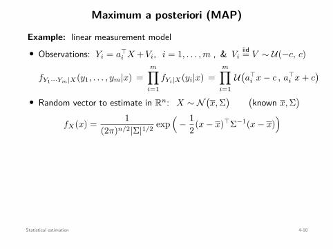
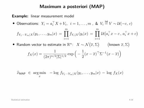
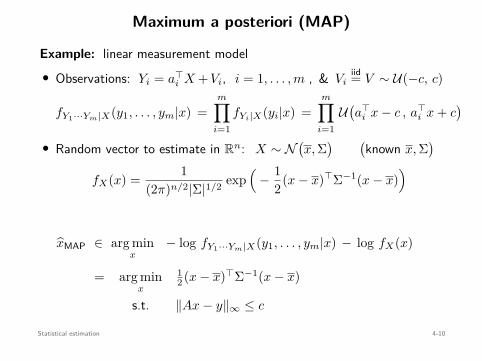
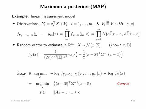

Maximum a posteriori (MAP)
LASSO:
• Observations: Yi = a⊤i X + Vi, i = 1, . . . , m, with
Viiid= V ∼ N (0, σ2)
• Random vector to estimate X ∈ Rn has iid Laplacian entries L(0, b)
xMAP ∈ arg minx
12
∥∥y − Ax∥∥2
2 + σ2
b∥x∥1
Known as basis pursuit denoising or LASSO (Convex)
Statistical estimation 4-11
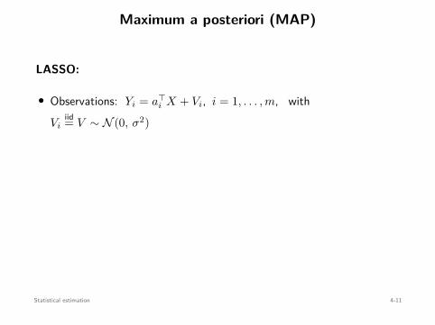
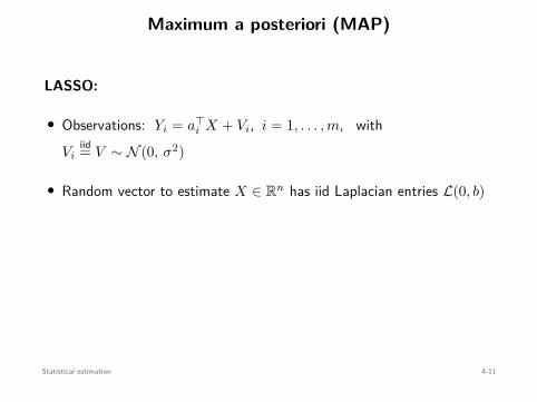
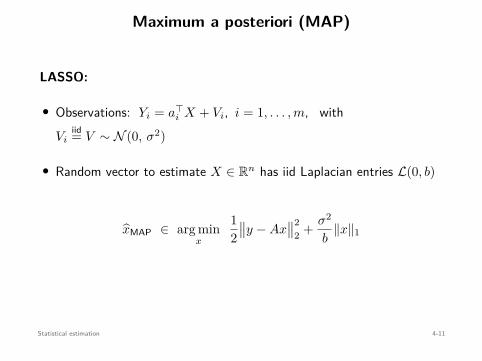
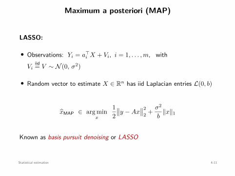
Maximum a posteriori (MAP)
LASSO:
• Observations: Yi = a⊤i X + Vi, i = 1, . . . , m, with
Viiid= V ∼ N (0, σ2)
• Random vector to estimate X ∈ Rn has iid Laplacian entries L(0, b)
xMAP ∈ arg minx
12
∥∥y − Ax∥∥2
2 + σ2
b∥x∥1
Known as basis pursuit denoising or LASSO
(Convex)
Statistical estimation 4-11
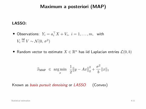
Maximum a posteriori (MAP)
LASSO:
• Observations: Yi = a⊤i X + Vi, i = 1, . . . , m, with
Viiid= V ∼ N (0, σ2)
• Random vector to estimate X ∈ Rn has iid Laplacian entries L(0, b)
xMAP ∈ arg minx
12
∥∥y − Ax∥∥2
2 + σ2
b∥x∥1
Known as basis pursuit denoising or LASSO (Convex)
Statistical estimation 4-11

Nonparametric estimation
ML and MAP allow estimating parameters of given distributions
What about estimating non-canonical distributions?
Example:
X: discrete RV taking values on 100 equidistant points in [−1, 1]
EX EX2E[3X3 − 2X]
P(X < 0)−1 0 1
We requireEX ∈ [−0.1, 0.1] EX2 ∈ [0.5, 0.6]
E[3X3 − 2X
]∈ [−0.3, −0.2]
P(X < 0
)∈ [0.3, 0.4]
Find a distribution satisfying these constraints & with maximum entropy
Statistical estimation 4-12
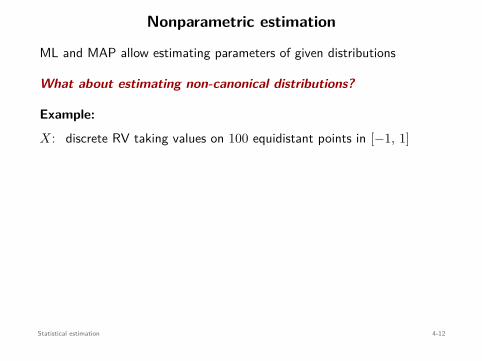
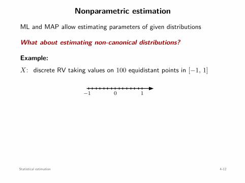
Nonparametric estimation
ML and MAP allow estimating parameters of given distributions
What about estimating non-canonical distributions?
Example:
X: discrete RV taking values on 100 equidistant points in [−1, 1]
EX EX2E[3X3 − 2X]
P(X < 0)
−1 0 1
We requireEX ∈ [−0.1, 0.1] EX2 ∈ [0.5, 0.6]
E[3X3 − 2X
]∈ [−0.3, −0.2]
P(X < 0
)∈ [0.3, 0.4]
Find a distribution satisfying these constraints & with maximum entropy
Statistical estimation 4-12
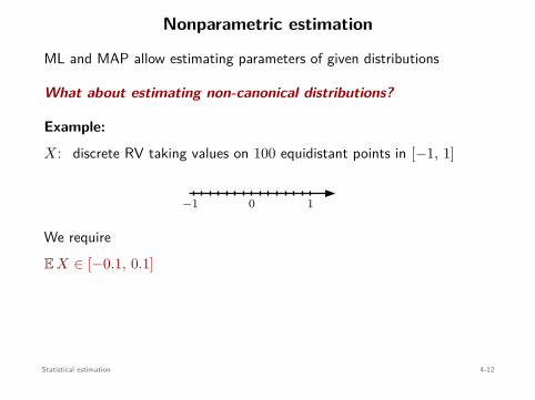
Nonparametric estimation
ML and MAP allow estimating parameters of given distributions
What about estimating non-canonical distributions?
Example:
X: discrete RV taking values on 100 equidistant points in [−1, 1]
EX EX2E[3X3 − 2X]
P(X < 0)
−1 0 1
We requireEX ∈ [−0.1, 0.1]
EX2 ∈ [0.5, 0.6]
E[3X3 − 2X
]∈ [−0.3, −0.2]
P(X < 0
)∈ [0.3, 0.4]
Find a distribution satisfying these constraints & with maximum entropy
Statistical estimation 4-12
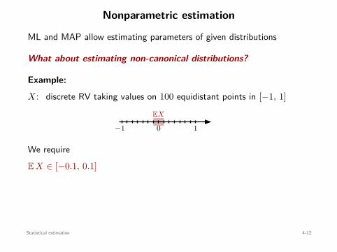
Nonparametric estimation
ML and MAP allow estimating parameters of given distributions
What about estimating non-canonical distributions?
Example:
X: discrete RV taking values on 100 equidistant points in [−1, 1]
EX
EX2E[3X3 − 2X]
P(X < 0)
−1 0 1
We requireEX ∈ [−0.1, 0.1]
EX2 ∈ [0.5, 0.6]
E[3X3 − 2X
]∈ [−0.3, −0.2]
P(X < 0
)∈ [0.3, 0.4]
Find a distribution satisfying these constraints & with maximum entropy
Statistical estimation 4-12
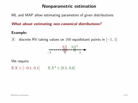
Nonparametric estimation
ML and MAP allow estimating parameters of given distributions
What about estimating non-canonical distributions?
Example:
X: discrete RV taking values on 100 equidistant points in [−1, 1]
EX EX2
E[3X3 − 2X]
P(X < 0)
−1 0 1
We requireEX ∈ [−0.1, 0.1] EX2 ∈ [0.5, 0.6]
E[3X3 − 2X
]∈ [−0.3, −0.2]
P(X < 0
)∈ [0.3, 0.4]
Find a distribution satisfying these constraints & with maximum entropy
Statistical estimation 4-12
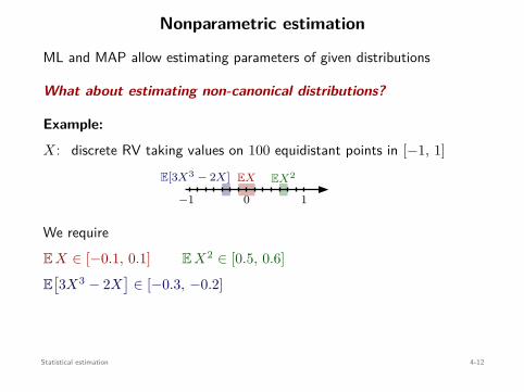
Nonparametric estimation
ML and MAP allow estimating parameters of given distributions
What about estimating non-canonical distributions?
Example:
X: discrete RV taking values on 100 equidistant points in [−1, 1]
EX EX2E[3X3 − 2X]
P(X < 0)
−1 0 1
We requireEX ∈ [−0.1, 0.1] EX2 ∈ [0.5, 0.6]
E[3X3 − 2X
]∈ [−0.3, −0.2]
P(X < 0
)∈ [0.3, 0.4]
Find a distribution satisfying these constraints & with maximum entropy
Statistical estimation 4-12
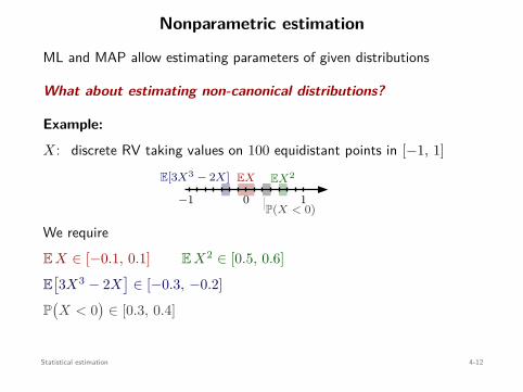
Nonparametric estimation
ML and MAP allow estimating parameters of given distributions
What about estimating non-canonical distributions?
Example:
X: discrete RV taking values on 100 equidistant points in [−1, 1]
EX EX2E[3X3 − 2X]
P(X < 0)−1 0 1
We requireEX ∈ [−0.1, 0.1] EX2 ∈ [0.5, 0.6]
E[3X3 − 2X
]∈ [−0.3, −0.2]
P(X < 0
)∈ [0.3, 0.4]
Find a distribution satisfying these constraints & with maximum entropy
Statistical estimation 4-12
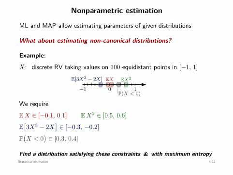
Nonparametric estimation
ML and MAP allow estimating parameters of given distributions
What about estimating non-canonical distributions?
Example:
X: discrete RV taking values on 100 equidistant points in [−1, 1]
EX EX2E[3X3 − 2X]
P(X < 0)−1 0 1
We requireEX ∈ [−0.1, 0.1] EX2 ∈ [0.5, 0.6]
E[3X3 − 2X
]∈ [−0.3, −0.2]
P(X < 0
)∈ [0.3, 0.4]
Find a distribution satisfying these constraints & with maximum entropyStatistical estimation 4-12
Nonparametric estimation
α = (−1, −0.9798, . . . , 0.9798, 1) ∈ R100 values that X takesp ∈ R100 such that pi = P(X = αi)
p: pmf =⇒ belongs to the probability simplex
p ∈ ∆n :=
x ∈ Rn : x ≥ 0n , 1⊤n x = 1
Rn
∆n
EX ∈ [−0.1, 0.1] ⇐⇒ −0.1 ≤ α⊤p ≤ 0.1
EX2 ∈ [0.5, 0.6] ⇐⇒ 0.5 ≤ β⊤p ≤ 0.6 βi = α2i
E[3X3 − 2X
]∈ [−0.3, −0.2] ⇐⇒ −0.3 ≤ γ⊤p ≤ −0.2 γi = 3α2
i − 2αi
P(X < 0
)∈ [0.3, 0.4] ⇐⇒ 0.3 ≤ σ⊤p ≤ 0.4 σi = 1 if i < 50
σi = 0 if i ≥ 50All constraints are linear inequalities in p!
Statistical estimation 4-13
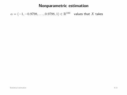
Nonparametric estimation
α = (−1, −0.9798, . . . , 0.9798, 1) ∈ R100 values that X takes
p ∈ R100 such that pi = P(X = αi)
p: pmf =⇒ belongs to the probability simplex
p ∈ ∆n :=
x ∈ Rn : x ≥ 0n , 1⊤n x = 1
Rn
∆n
EX ∈ [−0.1, 0.1] ⇐⇒ −0.1 ≤ α⊤p ≤ 0.1
EX2 ∈ [0.5, 0.6] ⇐⇒ 0.5 ≤ β⊤p ≤ 0.6 βi = α2i
E[3X3 − 2X
]∈ [−0.3, −0.2] ⇐⇒ −0.3 ≤ γ⊤p ≤ −0.2 γi = 3α2
i − 2αi
P(X < 0
)∈ [0.3, 0.4] ⇐⇒ 0.3 ≤ σ⊤p ≤ 0.4 σi = 1 if i < 50
σi = 0 if i ≥ 50All constraints are linear inequalities in p!
Statistical estimation 4-13
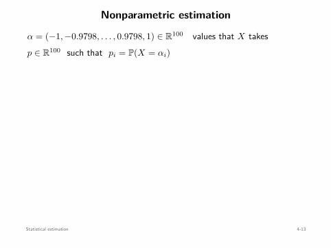
Nonparametric estimation
α = (−1, −0.9798, . . . , 0.9798, 1) ∈ R100 values that X takesp ∈ R100 such that pi = P(X = αi)
p: pmf =⇒ belongs to the probability simplex
p ∈ ∆n :=
x ∈ Rn : x ≥ 0n , 1⊤n x = 1
Rn
∆n
EX ∈ [−0.1, 0.1] ⇐⇒ −0.1 ≤ α⊤p ≤ 0.1
EX2 ∈ [0.5, 0.6] ⇐⇒ 0.5 ≤ β⊤p ≤ 0.6 βi = α2i
E[3X3 − 2X
]∈ [−0.3, −0.2] ⇐⇒ −0.3 ≤ γ⊤p ≤ −0.2 γi = 3α2
i − 2αi
P(X < 0
)∈ [0.3, 0.4] ⇐⇒ 0.3 ≤ σ⊤p ≤ 0.4 σi = 1 if i < 50
σi = 0 if i ≥ 50All constraints are linear inequalities in p!
Statistical estimation 4-13
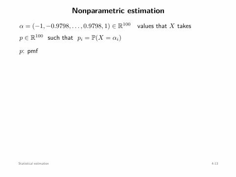
Nonparametric estimation
α = (−1, −0.9798, . . . , 0.9798, 1) ∈ R100 values that X takesp ∈ R100 such that pi = P(X = αi)
p: pmf
=⇒ belongs to the probability simplex
p ∈ ∆n :=
x ∈ Rn : x ≥ 0n , 1⊤n x = 1
Rn
∆n
EX ∈ [−0.1, 0.1] ⇐⇒ −0.1 ≤ α⊤p ≤ 0.1
EX2 ∈ [0.5, 0.6] ⇐⇒ 0.5 ≤ β⊤p ≤ 0.6 βi = α2i
E[3X3 − 2X
]∈ [−0.3, −0.2] ⇐⇒ −0.3 ≤ γ⊤p ≤ −0.2 γi = 3α2
i − 2αi
P(X < 0
)∈ [0.3, 0.4] ⇐⇒ 0.3 ≤ σ⊤p ≤ 0.4 σi = 1 if i < 50
σi = 0 if i ≥ 50All constraints are linear inequalities in p!
Statistical estimation 4-13
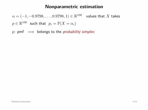
Nonparametric estimation
α = (−1, −0.9798, . . . , 0.9798, 1) ∈ R100 values that X takesp ∈ R100 such that pi = P(X = αi)
p: pmf =⇒ belongs to the probability simplex
p ∈ ∆n :=
x ∈ Rn : x ≥ 0n , 1⊤n x = 1
Rn
∆n
EX ∈ [−0.1, 0.1] ⇐⇒ −0.1 ≤ α⊤p ≤ 0.1
EX2 ∈ [0.5, 0.6] ⇐⇒ 0.5 ≤ β⊤p ≤ 0.6 βi = α2i
E[3X3 − 2X
]∈ [−0.3, −0.2] ⇐⇒ −0.3 ≤ γ⊤p ≤ −0.2 γi = 3α2
i − 2αi
P(X < 0
)∈ [0.3, 0.4] ⇐⇒ 0.3 ≤ σ⊤p ≤ 0.4 σi = 1 if i < 50
σi = 0 if i ≥ 50All constraints are linear inequalities in p!
Statistical estimation 4-13
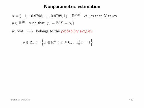
Nonparametric estimation
α = (−1, −0.9798, . . . , 0.9798, 1) ∈ R100 values that X takesp ∈ R100 such that pi = P(X = αi)
p: pmf =⇒ belongs to the probability simplex
p ∈ ∆n :=
x ∈ Rn : x ≥ 0n , 1⊤n x = 1
Rn
∆n
EX ∈ [−0.1, 0.1] ⇐⇒ −0.1 ≤ α⊤p ≤ 0.1
EX2 ∈ [0.5, 0.6] ⇐⇒ 0.5 ≤ β⊤p ≤ 0.6 βi = α2i
E[3X3 − 2X
]∈ [−0.3, −0.2] ⇐⇒ −0.3 ≤ γ⊤p ≤ −0.2 γi = 3α2
i − 2αi
P(X < 0
)∈ [0.3, 0.4] ⇐⇒ 0.3 ≤ σ⊤p ≤ 0.4 σi = 1 if i < 50
σi = 0 if i ≥ 50All constraints are linear inequalities in p!
Statistical estimation 4-13
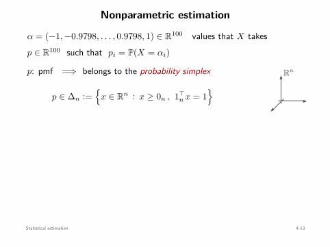
Nonparametric estimation
α = (−1, −0.9798, . . . , 0.9798, 1) ∈ R100 values that X takesp ∈ R100 such that pi = P(X = αi)
p: pmf =⇒ belongs to the probability simplex
p ∈ ∆n :=
x ∈ Rn : x ≥ 0n , 1⊤n x = 1
Rn
∆n
EX ∈ [−0.1, 0.1] ⇐⇒ −0.1 ≤ α⊤p ≤ 0.1
EX2 ∈ [0.5, 0.6] ⇐⇒ 0.5 ≤ β⊤p ≤ 0.6 βi = α2i
E[3X3 − 2X
]∈ [−0.3, −0.2] ⇐⇒ −0.3 ≤ γ⊤p ≤ −0.2 γi = 3α2
i − 2αi
P(X < 0
)∈ [0.3, 0.4] ⇐⇒ 0.3 ≤ σ⊤p ≤ 0.4 σi = 1 if i < 50
σi = 0 if i ≥ 50All constraints are linear inequalities in p!
Statistical estimation 4-13
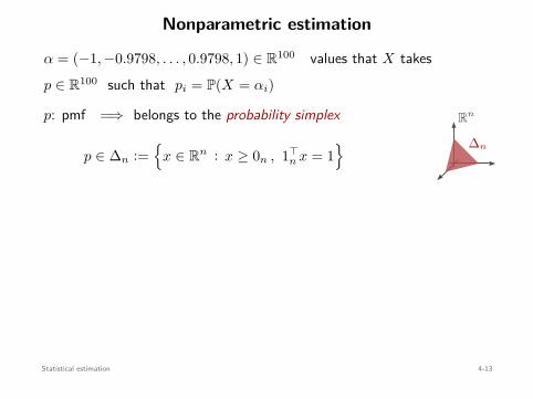
Nonparametric estimation
α = (−1, −0.9798, . . . , 0.9798, 1) ∈ R100 values that X takesp ∈ R100 such that pi = P(X = αi)
p: pmf =⇒ belongs to the probability simplex
p ∈ ∆n :=
x ∈ Rn : x ≥ 0n , 1⊤n x = 1
Rn
∆n
EX ∈ [−0.1, 0.1] ⇐⇒ −0.1 ≤ α⊤p ≤ 0.1
EX2 ∈ [0.5, 0.6] ⇐⇒ 0.5 ≤ β⊤p ≤ 0.6 βi = α2i
E[3X3 − 2X
]∈ [−0.3, −0.2] ⇐⇒ −0.3 ≤ γ⊤p ≤ −0.2 γi = 3α2
i − 2αi
P(X < 0
)∈ [0.3, 0.4] ⇐⇒ 0.3 ≤ σ⊤p ≤ 0.4 σi = 1 if i < 50
σi = 0 if i ≥ 50All constraints are linear inequalities in p!
Statistical estimation 4-13
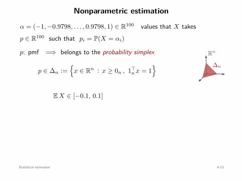
Nonparametric estimation
α = (−1, −0.9798, . . . , 0.9798, 1) ∈ R100 values that X takesp ∈ R100 such that pi = P(X = αi)
p: pmf =⇒ belongs to the probability simplex
p ∈ ∆n :=
x ∈ Rn : x ≥ 0n , 1⊤n x = 1
Rn
∆n
EX ∈ [−0.1, 0.1]
⇐⇒ −0.1 ≤ α⊤p ≤ 0.1
EX2 ∈ [0.5, 0.6] ⇐⇒ 0.5 ≤ β⊤p ≤ 0.6 βi = α2i
E[3X3 − 2X
]∈ [−0.3, −0.2] ⇐⇒ −0.3 ≤ γ⊤p ≤ −0.2 γi = 3α2
i − 2αi
P(X < 0
)∈ [0.3, 0.4] ⇐⇒ 0.3 ≤ σ⊤p ≤ 0.4 σi = 1 if i < 50
σi = 0 if i ≥ 50All constraints are linear inequalities in p!
Statistical estimation 4-13
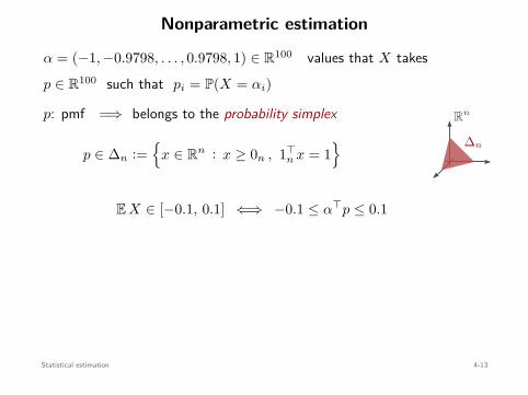
Nonparametric estimation
α = (−1, −0.9798, . . . , 0.9798, 1) ∈ R100 values that X takesp ∈ R100 such that pi = P(X = αi)
p: pmf =⇒ belongs to the probability simplex
p ∈ ∆n :=
x ∈ Rn : x ≥ 0n , 1⊤n x = 1
Rn
∆n
EX ∈ [−0.1, 0.1] ⇐⇒ −0.1 ≤ α⊤p ≤ 0.1
EX2 ∈ [0.5, 0.6] ⇐⇒ 0.5 ≤ β⊤p ≤ 0.6 βi = α2i
E[3X3 − 2X
]∈ [−0.3, −0.2] ⇐⇒ −0.3 ≤ γ⊤p ≤ −0.2 γi = 3α2
i − 2αi
P(X < 0
)∈ [0.3, 0.4] ⇐⇒ 0.3 ≤ σ⊤p ≤ 0.4 σi = 1 if i < 50
σi = 0 if i ≥ 50All constraints are linear inequalities in p!
Statistical estimation 4-13
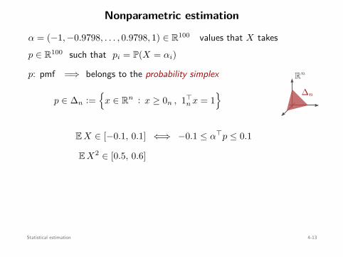
Nonparametric estimation
α = (−1, −0.9798, . . . , 0.9798, 1) ∈ R100 values that X takesp ∈ R100 such that pi = P(X = αi)
p: pmf =⇒ belongs to the probability simplex
p ∈ ∆n :=
x ∈ Rn : x ≥ 0n , 1⊤n x = 1
Rn
∆n
EX ∈ [−0.1, 0.1] ⇐⇒ −0.1 ≤ α⊤p ≤ 0.1
EX2 ∈ [0.5, 0.6]
⇐⇒ 0.5 ≤ β⊤p ≤ 0.6 βi = α2i
E[3X3 − 2X
]∈ [−0.3, −0.2] ⇐⇒ −0.3 ≤ γ⊤p ≤ −0.2 γi = 3α2
i − 2αi
P(X < 0
)∈ [0.3, 0.4] ⇐⇒ 0.3 ≤ σ⊤p ≤ 0.4 σi = 1 if i < 50
σi = 0 if i ≥ 50All constraints are linear inequalities in p!
Statistical estimation 4-13
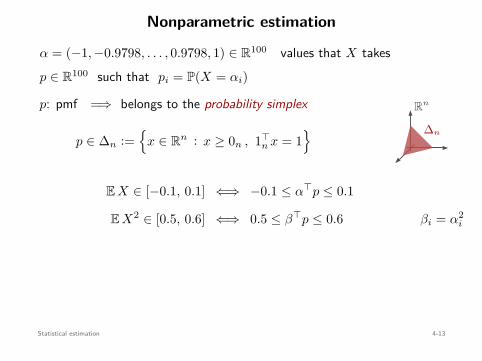
Nonparametric estimation
α = (−1, −0.9798, . . . , 0.9798, 1) ∈ R100 values that X takesp ∈ R100 such that pi = P(X = αi)
p: pmf =⇒ belongs to the probability simplex
p ∈ ∆n :=
x ∈ Rn : x ≥ 0n , 1⊤n x = 1
Rn
∆n
EX ∈ [−0.1, 0.1] ⇐⇒ −0.1 ≤ α⊤p ≤ 0.1
EX2 ∈ [0.5, 0.6] ⇐⇒ 0.5 ≤ β⊤p ≤ 0.6 βi = α2i
E[3X3 − 2X
]∈ [−0.3, −0.2] ⇐⇒ −0.3 ≤ γ⊤p ≤ −0.2 γi = 3α2
i − 2αi
P(X < 0
)∈ [0.3, 0.4] ⇐⇒ 0.3 ≤ σ⊤p ≤ 0.4 σi = 1 if i < 50
σi = 0 if i ≥ 50All constraints are linear inequalities in p!
Statistical estimation 4-13
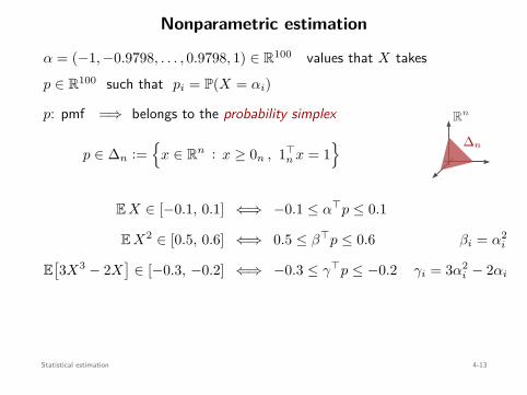
Nonparametric estimation
α = (−1, −0.9798, . . . , 0.9798, 1) ∈ R100 values that X takesp ∈ R100 such that pi = P(X = αi)
p: pmf =⇒ belongs to the probability simplex
p ∈ ∆n :=
x ∈ Rn : x ≥ 0n , 1⊤n x = 1
Rn
∆n
EX ∈ [−0.1, 0.1] ⇐⇒ −0.1 ≤ α⊤p ≤ 0.1
EX2 ∈ [0.5, 0.6] ⇐⇒ 0.5 ≤ β⊤p ≤ 0.6 βi = α2i
E[3X3 − 2X
]∈ [−0.3, −0.2] ⇐⇒ −0.3 ≤ γ⊤p ≤ −0.2 γi = 3α2
i − 2αi
P(X < 0
)∈ [0.3, 0.4] ⇐⇒ 0.3 ≤ σ⊤p ≤ 0.4 σi = 1 if i < 50
σi = 0 if i ≥ 50All constraints are linear inequalities in p!
Statistical estimation 4-13
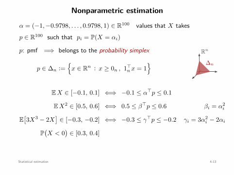
Nonparametric estimation
α = (−1, −0.9798, . . . , 0.9798, 1) ∈ R100 values that X takesp ∈ R100 such that pi = P(X = αi)
p: pmf =⇒ belongs to the probability simplex
p ∈ ∆n :=
x ∈ Rn : x ≥ 0n , 1⊤n x = 1
Rn
∆n
EX ∈ [−0.1, 0.1] ⇐⇒ −0.1 ≤ α⊤p ≤ 0.1
EX2 ∈ [0.5, 0.6] ⇐⇒ 0.5 ≤ β⊤p ≤ 0.6 βi = α2i
E[3X3 − 2X
]∈ [−0.3, −0.2] ⇐⇒ −0.3 ≤ γ⊤p ≤ −0.2 γi = 3α2
i − 2αi
P(X < 0
)∈ [0.3, 0.4]
⇐⇒ 0.3 ≤ σ⊤p ≤ 0.4 σi = 1 if i < 50
σi = 0 if i ≥ 50All constraints are linear inequalities in p!
Statistical estimation 4-13
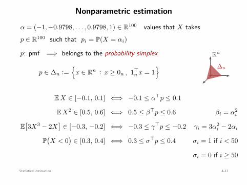
Nonparametric estimation
α = (−1, −0.9798, . . . , 0.9798, 1) ∈ R100 values that X takesp ∈ R100 such that pi = P(X = αi)
p: pmf =⇒ belongs to the probability simplex
p ∈ ∆n :=
x ∈ Rn : x ≥ 0n , 1⊤n x = 1
Rn
∆n
EX ∈ [−0.1, 0.1] ⇐⇒ −0.1 ≤ α⊤p ≤ 0.1
EX2 ∈ [0.5, 0.6] ⇐⇒ 0.5 ≤ β⊤p ≤ 0.6 βi = α2i
E[3X3 − 2X
]∈ [−0.3, −0.2] ⇐⇒ −0.3 ≤ γ⊤p ≤ −0.2 γi = 3α2
i − 2αi
P(X < 0
)∈ [0.3, 0.4] ⇐⇒ 0.3 ≤ σ⊤p ≤ 0.4 σi = 1 if i < 50
σi = 0 if i ≥ 50
All constraints are linear inequalities in p!
Statistical estimation 4-13
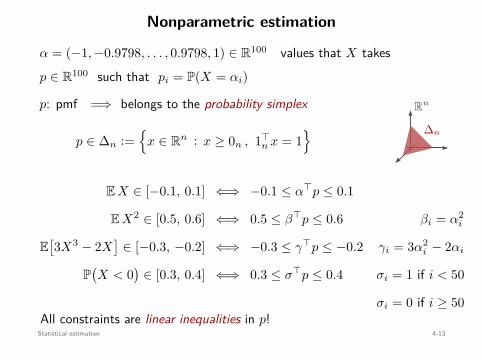
Nonparametric estimation
α = (−1, −0.9798, . . . , 0.9798, 1) ∈ R100 values that X takesp ∈ R100 such that pi = P(X = αi)
p: pmf =⇒ belongs to the probability simplex
p ∈ ∆n :=
x ∈ Rn : x ≥ 0n , 1⊤n x = 1
Rn
∆n
EX ∈ [−0.1, 0.1] ⇐⇒ −0.1 ≤ α⊤p ≤ 0.1
EX2 ∈ [0.5, 0.6] ⇐⇒ 0.5 ≤ β⊤p ≤ 0.6 βi = α2i
E[3X3 − 2X
]∈ [−0.3, −0.2] ⇐⇒ −0.3 ≤ γ⊤p ≤ −0.2 γi = 3α2
i − 2αi
P(X < 0
)∈ [0.3, 0.4] ⇐⇒ 0.3 ≤ σ⊤p ≤ 0.4 σi = 1 if i < 50
σi = 0 if i ≥ 50All constraints are linear inequalities in p!
Statistical estimation 4-13
Nonparametric estimation
Maximize entropy
= minimize negative entropy:
−H(p) :=n∑
i=1pi log pi
Convex because d2
dx2 x log x = 1x > 0, for all x > 0
Optimization problem: (convex)
minimizep∈R100
∑ni=1 pi log pi
subject to −0.1 ≤ α⊤p ≤ 0.1
0.5 ≤ β⊤p ≤ 0.6
−0.3 ≤ γ⊤p ≤ −0.2
0.3 ≤ σ⊤p ≤ 0.4
Statistical estimation 4-14
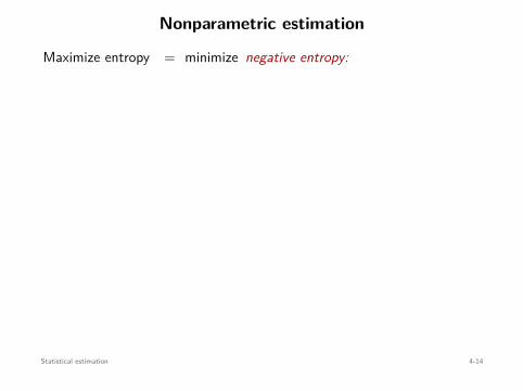
Nonparametric estimation
Maximize entropy = minimize negative entropy:
−H(p) :=n∑
i=1pi log pi
Convex because d2
dx2 x log x = 1x > 0, for all x > 0
Optimization problem: (convex)
minimizep∈R100
∑ni=1 pi log pi
subject to −0.1 ≤ α⊤p ≤ 0.1
0.5 ≤ β⊤p ≤ 0.6
−0.3 ≤ γ⊤p ≤ −0.2
0.3 ≤ σ⊤p ≤ 0.4
Statistical estimation 4-14
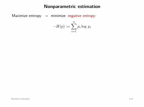
Nonparametric estimation
Maximize entropy = minimize negative entropy:
−H(p) :=n∑
i=1pi log pi
Convex because d2
dx2 x log x = 1x > 0, for all x > 0
Optimization problem: (convex)
minimizep∈R100
∑ni=1 pi log pi
subject to −0.1 ≤ α⊤p ≤ 0.1
0.5 ≤ β⊤p ≤ 0.6
−0.3 ≤ γ⊤p ≤ −0.2
0.3 ≤ σ⊤p ≤ 0.4
Statistical estimation 4-14
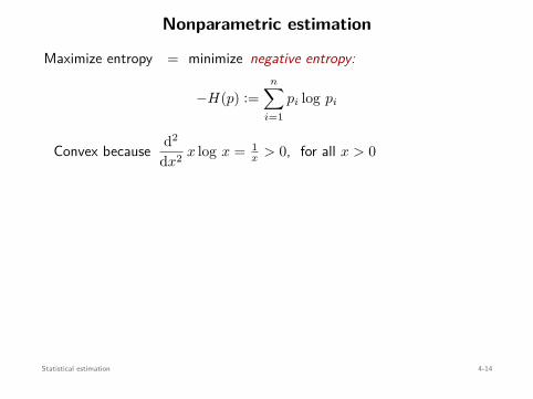
Nonparametric estimation
Maximize entropy = minimize negative entropy:
−H(p) :=n∑
i=1pi log pi
Convex because d2
dx2 x log x = 1x > 0, for all x > 0
Optimization problem: (convex)
minimizep∈R100
∑ni=1 pi log pi
subject to −0.1 ≤ α⊤p ≤ 0.1
0.5 ≤ β⊤p ≤ 0.6
−0.3 ≤ γ⊤p ≤ −0.2
0.3 ≤ σ⊤p ≤ 0.4
Statistical estimation 4-14
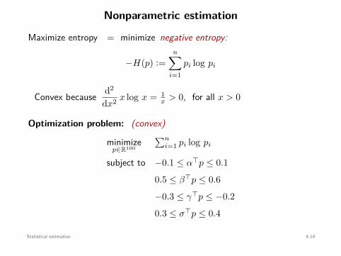
Nonparametric estimation
Maximize entropy = minimize negative entropy:
−H(p) :=n∑
i=1pi log pi
Convex because d2
dx2 x log x = 1x > 0, for all x > 0
Optimization problem: (convex)
minimizep∈R100
∑ni=1 pi log pi
subject to −0.1 ≤ α⊤p ≤ 0.1
0.5 ≤ β⊤p ≤ 0.6
−0.3 ≤ γ⊤p ≤ −0.2
0.3 ≤ σ⊤p ≤ 0.4
Statistical estimation 4-14
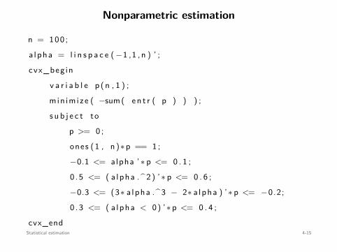
Nonparametric estimation
n = 100 ;a lpha = l i n s p a c e ( −1 ,1 ,n ) ’ ;cvx_beg in
v a r i a b l e p (n , 1 ) ;m in im ize ( −sum( e n t r ( p ) ) ) ;s u b j e c t to
p >= 0 ;ones (1 , n )∗p == 1 ;−0.1 <= alpha ’∗ p <= 0 . 1 ;0 . 5 <= ( a lpha . ^ 2 ) ’∗ p <= 0 . 6 ;−0.3 <= (3∗ a lpha .^3 − 2∗ a lpha ) ’∗ p <= −0.2;0 . 3 <= ( a lpha < 0) ’∗ p <= 0 . 4 ;
cvx_endStatistical estimation 4-15
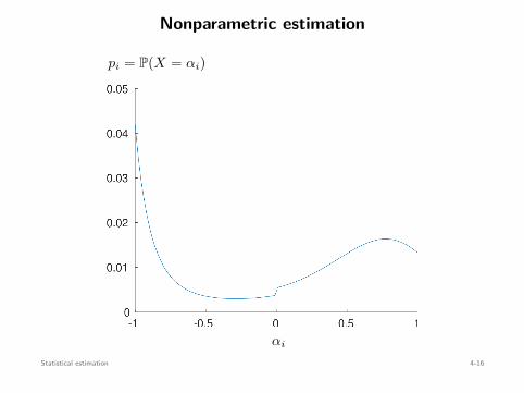
Nonparametric estimation
pi = P(X = αi)
αi
Statistical estimation 4-16
Hypothesis testing & optimal detection
X : discrete random variable w/ probability mass function (pmf) pθ
X ∈ 1, . . . , n
θ ∈ 1, . . . , mx
p1(x)
x
p2(x)
P =
P(X = 1 | θ = 1) P(X = 1 | θ = 2) · · · P(X = 1 | θ = m)
P(X = 2 | θ = 1) P(X = 2 | θ = 2) · · · P(X = 2 | θ = m)...
......
P(X = n | θ = 1) P(X = n | θ = 2) · · · P(X = n | θ = m)
∈ Rn×m
Goal: Estimate θ based on an observation of X
Statistical estimation 4-17
Hypothesis testing & optimal detection
X : discrete random variable w/ probability mass function (pmf) pθ
X ∈ 1, . . . , n
θ ∈ 1, . . . , m
x
p1(x)
x
p2(x)
P =
P(X = 1 | θ = 1) P(X = 1 | θ = 2) · · · P(X = 1 | θ = m)
P(X = 2 | θ = 1) P(X = 2 | θ = 2) · · · P(X = 2 | θ = m)...
......
P(X = n | θ = 1) P(X = n | θ = 2) · · · P(X = n | θ = m)
∈ Rn×m
Goal: Estimate θ based on an observation of X
Statistical estimation 4-17
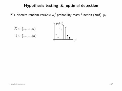
Hypothesis testing & optimal detection
X : discrete random variable w/ probability mass function (pmf) pθ
X ∈ 1, . . . , n
θ ∈ 1, . . . , mx
p1(x)
x
p2(x)
P =
P(X = 1 | θ = 1) P(X = 1 | θ = 2) · · · P(X = 1 | θ = m)
P(X = 2 | θ = 1) P(X = 2 | θ = 2) · · · P(X = 2 | θ = m)...
......
P(X = n | θ = 1) P(X = n | θ = 2) · · · P(X = n | θ = m)
∈ Rn×m
Goal: Estimate θ based on an observation of X
Statistical estimation 4-17
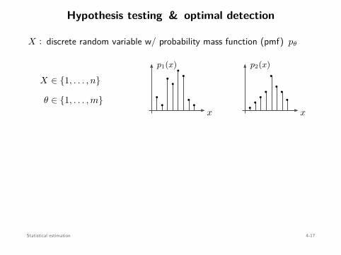
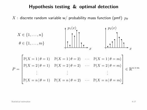
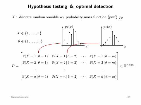
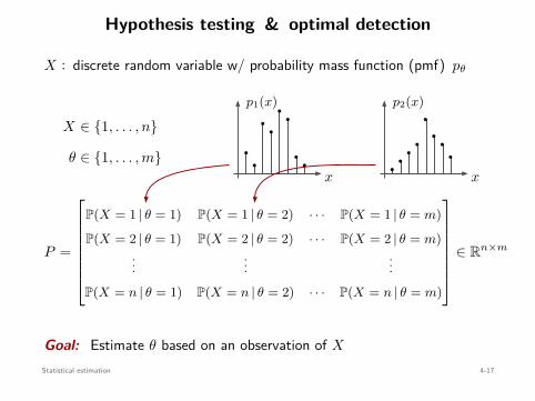

Detector:
Ψ : 1, . . . , n
︸ ︷︷ ︸X
−→ 1, . . . , m
︸ ︷︷ ︸θ
Example: maximum likelihood detector
θML = ΨML(x) = arg maxj
P(X = x | θ = j
)
Randomized detector: Random variable θ whose pmf depends on X
T =
P(θ = 1 | X = 1) P(θ = 1 | X = 2) · · · P(θ = 1 | X = n)
P(θ = 2 | X = 1) P(θ = 2 | X = 2) · · · P(θ = 2 | X = n)...
......
P(θ = m | X = 1) P(θ = m | X = 2) · · · P(θ = m | X = n)
∈ Rm×n
Each column ti ∈ Rm satisfies 1⊤mti = 1, ti ≥ 0
If each ti is a canonical vector (0, . . . , 1, . . . , 0), then T is deterministic
Statistical estimation 4-18
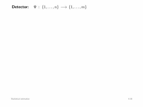
Detector: Ψ : 1, . . . , n
︸ ︷︷ ︸X
−→ 1, . . . , m
︸ ︷︷ ︸θ
Example: maximum likelihood detector
θML = ΨML(x) = arg maxj
P(X = x | θ = j
)
Randomized detector: Random variable θ whose pmf depends on X
T =
P(θ = 1 | X = 1) P(θ = 1 | X = 2) · · · P(θ = 1 | X = n)
P(θ = 2 | X = 1) P(θ = 2 | X = 2) · · · P(θ = 2 | X = n)...
......
P(θ = m | X = 1) P(θ = m | X = 2) · · · P(θ = m | X = n)
∈ Rm×n
Each column ti ∈ Rm satisfies 1⊤mti = 1, ti ≥ 0
If each ti is a canonical vector (0, . . . , 1, . . . , 0), then T is deterministic
Statistical estimation 4-18
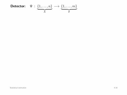
Detector: Ψ : 1, . . . , n︸ ︷︷ ︸X
−→ 1, . . . , m︸ ︷︷ ︸θ
Example: maximum likelihood detector
θML = ΨML(x) = arg maxj
P(X = x | θ = j
)
Randomized detector: Random variable θ whose pmf depends on X
T =
P(θ = 1 | X = 1) P(θ = 1 | X = 2) · · · P(θ = 1 | X = n)
P(θ = 2 | X = 1) P(θ = 2 | X = 2) · · · P(θ = 2 | X = n)...
......
P(θ = m | X = 1) P(θ = m | X = 2) · · · P(θ = m | X = n)
∈ Rm×n
Each column ti ∈ Rm satisfies 1⊤mti = 1, ti ≥ 0
If each ti is a canonical vector (0, . . . , 1, . . . , 0), then T is deterministic
Statistical estimation 4-18
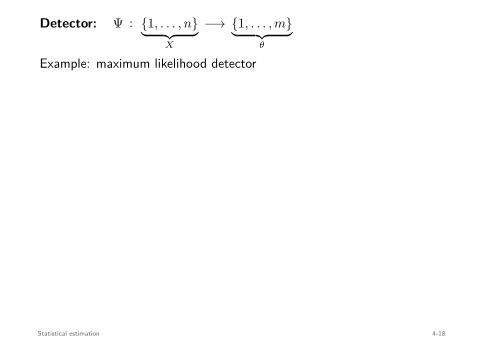
Detector: Ψ : 1, . . . , n︸ ︷︷ ︸X
−→ 1, . . . , m︸ ︷︷ ︸θ
Example: maximum likelihood detector
θML = ΨML(x) = arg maxj
P(X = x | θ = j
)
Randomized detector: Random variable θ whose pmf depends on X
T =
P(θ = 1 | X = 1) P(θ = 1 | X = 2) · · · P(θ = 1 | X = n)
P(θ = 2 | X = 1) P(θ = 2 | X = 2) · · · P(θ = 2 | X = n)...
......
P(θ = m | X = 1) P(θ = m | X = 2) · · · P(θ = m | X = n)
∈ Rm×n
Each column ti ∈ Rm satisfies 1⊤mti = 1, ti ≥ 0
If each ti is a canonical vector (0, . . . , 1, . . . , 0), then T is deterministic
Statistical estimation 4-18
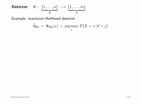
Detector: Ψ : 1, . . . , n︸ ︷︷ ︸X
−→ 1, . . . , m︸ ︷︷ ︸θ
Example: maximum likelihood detector
θML = ΨML(x) = arg maxj
P(X = x | θ = j
)
Randomized detector: Random variable θ whose pmf depends on X
T =
P(θ = 1 | X = 1) P(θ = 1 | X = 2) · · · P(θ = 1 | X = n)
P(θ = 2 | X = 1) P(θ = 2 | X = 2) · · · P(θ = 2 | X = n)...
......
P(θ = m | X = 1) P(θ = m | X = 2) · · · P(θ = m | X = n)
∈ Rm×n
Each column ti ∈ Rm satisfies 1⊤mti = 1, ti ≥ 0
If each ti is a canonical vector (0, . . . , 1, . . . , 0), then T is deterministic
Statistical estimation 4-18
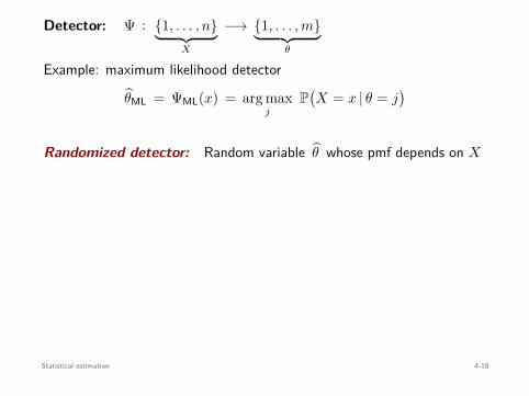
Detector: Ψ : 1, . . . , n︸ ︷︷ ︸X
−→ 1, . . . , m︸ ︷︷ ︸θ
Example: maximum likelihood detector
θML = ΨML(x) = arg maxj
P(X = x | θ = j
)
Randomized detector: Random variable θ whose pmf depends on X
T =
P(θ = 1 | X = 1) P(θ = 1 | X = 2) · · · P(θ = 1 | X = n)
P(θ = 2 | X = 1) P(θ = 2 | X = 2) · · · P(θ = 2 | X = n)...
......
P(θ = m | X = 1) P(θ = m | X = 2) · · · P(θ = m | X = n)
∈ Rm×n
Each column ti ∈ Rm satisfies 1⊤mti = 1, ti ≥ 0
If each ti is a canonical vector (0, . . . , 1, . . . , 0), then T is deterministic
Statistical estimation 4-18
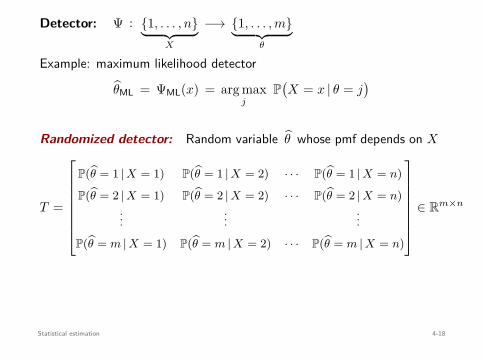
Detector: Ψ : 1, . . . , n︸ ︷︷ ︸X
−→ 1, . . . , m︸ ︷︷ ︸θ
Example: maximum likelihood detector
θML = ΨML(x) = arg maxj
P(X = x | θ = j
)
Randomized detector: Random variable θ whose pmf depends on X
T =
P(θ = 1 | X = 1) P(θ = 1 | X = 2) · · · P(θ = 1 | X = n)
P(θ = 2 | X = 1) P(θ = 2 | X = 2) · · · P(θ = 2 | X = n)...
......
P(θ = m | X = 1) P(θ = m | X = 2) · · · P(θ = m | X = n)
∈ Rm×n
Each column ti ∈ Rm satisfies 1⊤mti = 1, ti ≥ 0
If each ti is a canonical vector (0, . . . , 1, . . . , 0), then T is deterministic
Statistical estimation 4-18
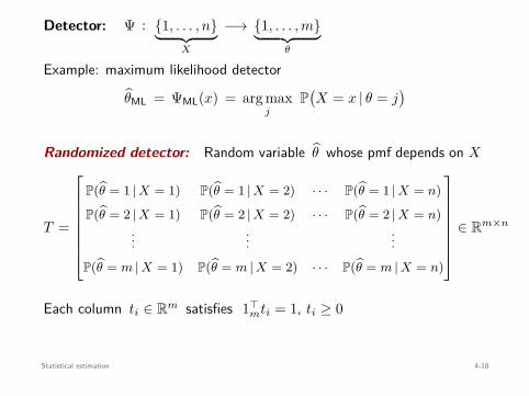
Detector: Ψ : 1, . . . , n︸ ︷︷ ︸X
−→ 1, . . . , m︸ ︷︷ ︸θ
Example: maximum likelihood detector
θML = ΨML(x) = arg maxj
P(X = x | θ = j
)
Randomized detector: Random variable θ whose pmf depends on X
T =
P(θ = 1 | X = 1) P(θ = 1 | X = 2) · · · P(θ = 1 | X = n)
P(θ = 2 | X = 1) P(θ = 2 | X = 2) · · · P(θ = 2 | X = n)...
......
P(θ = m | X = 1) P(θ = m | X = 2) · · · P(θ = m | X = n)
∈ Rm×n
Each column ti ∈ Rm satisfies 1⊤mti = 1, ti ≥ 0
If each ti is a canonical vector (0, . . . , 1, . . . , 0), then T is deterministic
Statistical estimation 4-18
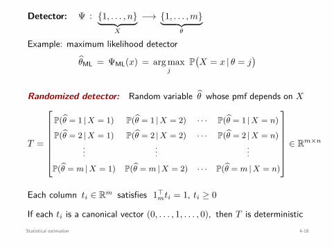
Detector: Ψ : 1, . . . , n︸ ︷︷ ︸X
−→ 1, . . . , m︸ ︷︷ ︸θ
Example: maximum likelihood detector
θML = ΨML(x) = arg maxj
P(X = x | θ = j
)
Randomized detector: Random variable θ whose pmf depends on X
T =
P(θ = 1 | X = 1) P(θ = 1 | X = 2) · · · P(θ = 1 | X = n)
P(θ = 2 | X = 1) P(θ = 2 | X = 2) · · · P(θ = 2 | X = n)...
......
P(θ = m | X = 1) P(θ = m | X = 2) · · · P(θ = m | X = n)
∈ Rm×n
Each column ti ∈ Rm satisfies 1⊤mti = 1, ti ≥ 0
If each ti is a canonical vector (0, . . . , 1, . . . , 0), then T is deterministicStatistical estimation 4-18
Detection probability matrix:
D := TP ∈ Rm×m
Dij =n∑
k=1P
(θ = i | X = k
)· P
(X = k | θ = j
)
= P(
θ = i
︸ ︷︷ ︸guess
| θ = j
︸ ︷︷ ︸true
)
Goal: Design T such that the Dij ’s, for i = j, are as small as possible
Multi-objective optimization
Statistical estimation 4-19
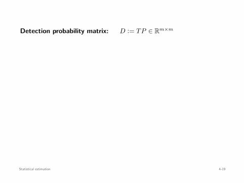
Detection probability matrix: D := TP ∈ Rm×m
Dij =n∑
k=1P
(θ = i | X = k
)· P
(X = k | θ = j
)
= P(
θ = i
︸ ︷︷ ︸guess
| θ = j
︸ ︷︷ ︸true
)
Goal: Design T such that the Dij ’s, for i = j, are as small as possible
Multi-objective optimization
Statistical estimation 4-19
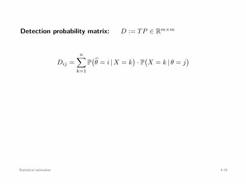
Detection probability matrix: D := TP ∈ Rm×m
Dij =n∑
k=1P
(θ = i | X = k
)· P
(X = k | θ = j
)
= P(
θ = i
︸ ︷︷ ︸guess
| θ = j
︸ ︷︷ ︸true
)
Goal: Design T such that the Dij ’s, for i = j, are as small as possible
Multi-objective optimization
Statistical estimation 4-19
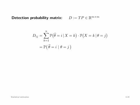
Detection probability matrix: D := TP ∈ Rm×m
Dij =n∑
k=1P
(θ = i | X = k
)· P
(X = k | θ = j
)
= P(
θ = i
︸ ︷︷ ︸guess
| θ = j
︸ ︷︷ ︸true
)
Goal: Design T such that the Dij ’s, for i = j, are as small as possible
Multi-objective optimization
Statistical estimation 4-19
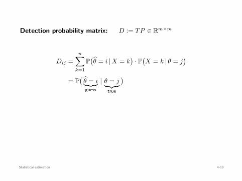
Detection probability matrix: D := TP ∈ Rm×m
Dij =n∑
k=1P
(θ = i | X = k
)· P
(X = k | θ = j
)
= P(
θ = i︸ ︷︷ ︸guess
| θ = j︸ ︷︷ ︸true
)
Goal: Design T such that the Dij ’s, for i = j, are as small as possible
Multi-objective optimization
Statistical estimation 4-19
Detection probability matrix: D := TP ∈ Rm×m
Dij =n∑
k=1P
(θ = i | X = k
)· P
(X = k | θ = j
)
= P(
θ = i︸ ︷︷ ︸guess
| θ = j︸ ︷︷ ︸true
)
Goal: Design T such that the Dij ’s, for i = j, are as small as possible
Multi-objective optimization
Statistical estimation 4-19
Detection probability matrix: D := TP ∈ Rm×m
Dij =n∑
k=1P
(θ = i | X = k
)· P
(X = k | θ = j
)
= P(
θ = i︸ ︷︷ ︸guess
| θ = j︸ ︷︷ ︸true
)
Goal: Design T such that the Dij ’s, for i = j, are as small as possible
Multi-objective optimization
Statistical estimation 4-19
Minimax detector
Note that
P(θ = j | θ = j
)= 1 − P
(θ = j | θ = j
)= 1 − Djj
Minimax detector:
minimizeT ∈Rm×n
maxj=i,...,m
1 − Djj(T )
subject to T ⊤1m = 1n , T ≥ 0
⇐⇒ minimizeT ∈Rm×n
maxj=i,...,m
1 − tr(TP eje⊤
j
)
subject to T ⊤1m = 1n , T ≥ 0
Convex
Statistical estimation 4-20
Minimax detector
Note that
P(θ = j | θ = j
)
= 1 − P(θ = j | θ = j
)= 1 − Djj
Minimax detector:
minimizeT ∈Rm×n
maxj=i,...,m
1 − Djj(T )
subject to T ⊤1m = 1n , T ≥ 0
⇐⇒ minimizeT ∈Rm×n
maxj=i,...,m
1 − tr(TP eje⊤
j
)
subject to T ⊤1m = 1n , T ≥ 0
Convex
Statistical estimation 4-20
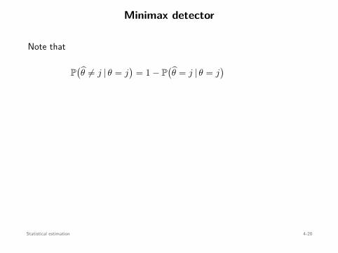
Minimax detector
Note that
P(θ = j | θ = j
)= 1 − P
(θ = j | θ = j
)
= 1 − Djj
Minimax detector:
minimizeT ∈Rm×n
maxj=i,...,m
1 − Djj(T )
subject to T ⊤1m = 1n , T ≥ 0
⇐⇒ minimizeT ∈Rm×n
maxj=i,...,m
1 − tr(TP eje⊤
j
)
subject to T ⊤1m = 1n , T ≥ 0
Convex
Statistical estimation 4-20
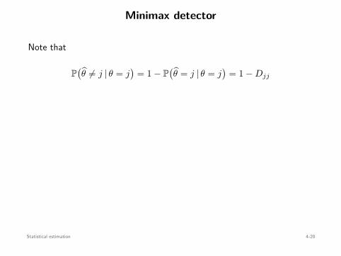
Minimax detector
Note that
P(θ = j | θ = j
)= 1 − P
(θ = j | θ = j
)= 1 − Djj
Minimax detector:
minimizeT ∈Rm×n
maxj=i,...,m
1 − Djj(T )
subject to T ⊤1m = 1n , T ≥ 0
⇐⇒ minimizeT ∈Rm×n
maxj=i,...,m
1 − tr(TP eje⊤
j
)
subject to T ⊤1m = 1n , T ≥ 0
Convex
Statistical estimation 4-20
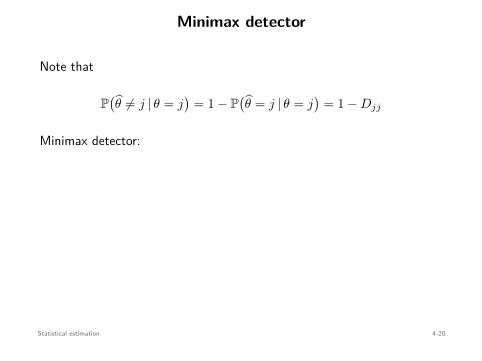
Minimax detector
Note that
P(θ = j | θ = j
)= 1 − P
(θ = j | θ = j
)= 1 − Djj
Minimax detector:
minimizeT ∈Rm×n
maxj=i,...,m
1 − Djj(T )
subject to T ⊤1m = 1n , T ≥ 0
⇐⇒ minimizeT ∈Rm×n
maxj=i,...,m
1 − tr(TP eje⊤
j
)
subject to T ⊤1m = 1n , T ≥ 0
Convex
Statistical estimation 4-20
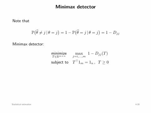
Minimax detector
Note that
P(θ = j | θ = j
)= 1 − P
(θ = j | θ = j
)= 1 − Djj
Minimax detector:
minimizeT ∈Rm×n
maxj=i,...,m
1 − Djj(T )
subject to T ⊤1m = 1n , T ≥ 0
⇐⇒ minimizeT ∈Rm×n
maxj=i,...,m
1 − tr(TP eje⊤
j
)
subject to T ⊤1m = 1n , T ≥ 0
Convex
Statistical estimation 4-20
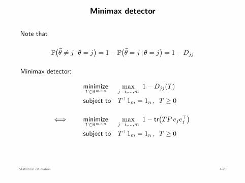
Minimax detector
Note that
P(θ = j | θ = j
)= 1 − P
(θ = j | θ = j
)= 1 − Djj
Minimax detector:
minimizeT ∈Rm×n
maxj=i,...,m
1 − Djj(T )
subject to T ⊤1m = 1n , T ≥ 0
⇐⇒ minimizeT ∈Rm×n
maxj=i,...,m
1 − tr(TP eje⊤
j
)
subject to T ⊤1m = 1n , T ≥ 0
Convex
Statistical estimation 4-20
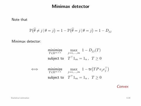
Minimax detector
Note that
P(θ = j | θ = j
)= 1 − P
(θ = j | θ = j
)= 1 − Djj
Minimax detector:
minimizeT ∈Rm×n
maxj=i,...,m
1 − Djj(T )
subject to T ⊤1m = 1n , T ≥ 0
⇐⇒ minimizeT ∈Rm×n
maxj=i,...,m
1 − tr(TP eje⊤
j
)
subject to T ⊤1m = 1n , T ≥ 0
Convex
Statistical estimation 4-20

Pareto-optimal detectors
Recall that we want to minimize all Dij = P(θ = i | θ = j
), for i = j
Scalarization: Fix W ∈ Rm×m w/ Wii = 0, and Wij > 0 for i = j
minimizeT
m∑
i=1
m∑
j=1WijDij(T )
subject to T ⊤1m = 1n , T ≥ 0
By varying W we can find Pareto optimal solutions
Observations:
• Constraints ⇐⇒ 1⊤mti = 1, ti ≥ 0, for i = 1, . . . , n
• Objective ⇐⇒ tr(W ⊤TP
)
= tr((WP ⊤)⊤T
)=
∑ni=1 c⊤
i ti
where ci: ith column of C := WP ⊤
Statistical estimation 4-21
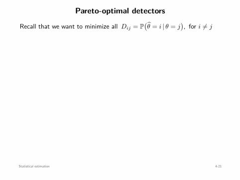
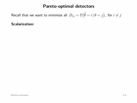
Pareto-optimal detectors
Recall that we want to minimize all Dij = P(θ = i | θ = j
), for i = j
Scalarization:
Fix W ∈ Rm×m w/ Wii = 0, and Wij > 0 for i = j
minimizeT
m∑
i=1
m∑
j=1WijDij(T )
subject to T ⊤1m = 1n , T ≥ 0
By varying W we can find Pareto optimal solutions
Observations:
• Constraints ⇐⇒ 1⊤mti = 1, ti ≥ 0, for i = 1, . . . , n
• Objective ⇐⇒ tr(W ⊤TP
)
= tr((WP ⊤)⊤T
)=
∑ni=1 c⊤
i ti
where ci: ith column of C := WP ⊤
Statistical estimation 4-21
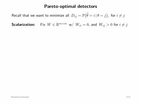
Pareto-optimal detectors
Recall that we want to minimize all Dij = P(θ = i | θ = j
), for i = j
Scalarization: Fix W ∈ Rm×m w/ Wii = 0, and Wij > 0 for i = j
minimizeT
m∑
i=1
m∑
j=1WijDij(T )
subject to T ⊤1m = 1n , T ≥ 0
By varying W we can find Pareto optimal solutions
Observations:
• Constraints ⇐⇒ 1⊤mti = 1, ti ≥ 0, for i = 1, . . . , n
• Objective ⇐⇒ tr(W ⊤TP
)
= tr((WP ⊤)⊤T
)=
∑ni=1 c⊤
i ti
where ci: ith column of C := WP ⊤
Statistical estimation 4-21
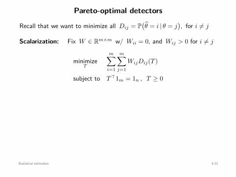
Pareto-optimal detectors
Recall that we want to minimize all Dij = P(θ = i | θ = j
), for i = j
Scalarization: Fix W ∈ Rm×m w/ Wii = 0, and Wij > 0 for i = j
minimizeT
m∑
i=1
m∑
j=1WijDij(T )
subject to T ⊤1m = 1n , T ≥ 0
By varying W we can find Pareto optimal solutions
Observations:
• Constraints ⇐⇒ 1⊤mti = 1, ti ≥ 0, for i = 1, . . . , n
• Objective ⇐⇒ tr(W ⊤TP
)
= tr((WP ⊤)⊤T
)=
∑ni=1 c⊤
i ti
where ci: ith column of C := WP ⊤
Statistical estimation 4-21
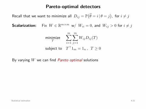
Pareto-optimal detectors
Recall that we want to minimize all Dij = P(θ = i | θ = j
), for i = j
Scalarization: Fix W ∈ Rm×m w/ Wii = 0, and Wij > 0 for i = j
minimizeT
m∑
i=1
m∑
j=1WijDij(T )
subject to T ⊤1m = 1n , T ≥ 0
By varying W we can find Pareto optimal solutions
Observations:
• Constraints ⇐⇒ 1⊤mti = 1, ti ≥ 0, for i = 1, . . . , n
• Objective ⇐⇒ tr(W ⊤TP
)
= tr((WP ⊤)⊤T
)=
∑ni=1 c⊤
i ti
where ci: ith column of C := WP ⊤
Statistical estimation 4-21
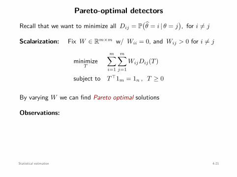
Pareto-optimal detectors
Recall that we want to minimize all Dij = P(θ = i | θ = j
), for i = j
Scalarization: Fix W ∈ Rm×m w/ Wii = 0, and Wij > 0 for i = j
minimizeT
m∑
i=1
m∑
j=1WijDij(T )
subject to T ⊤1m = 1n , T ≥ 0
By varying W we can find Pareto optimal solutions
Observations:
• Constraints ⇐⇒ 1⊤mti = 1, ti ≥ 0, for i = 1, . . . , n
• Objective ⇐⇒ tr(W ⊤TP
)
= tr((WP ⊤)⊤T
)=
∑ni=1 c⊤
i ti
where ci: ith column of C := WP ⊤
Statistical estimation 4-21
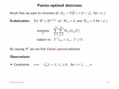
Pareto-optimal detectors
Recall that we want to minimize all Dij = P(θ = i | θ = j
), for i = j
Scalarization: Fix W ∈ Rm×m w/ Wii = 0, and Wij > 0 for i = j
minimizeT
m∑
i=1
m∑
j=1WijDij(T )
subject to T ⊤1m = 1n , T ≥ 0
By varying W we can find Pareto optimal solutions
Observations:
• Constraints ⇐⇒ 1⊤mti = 1, ti ≥ 0, for i = 1, . . . , n
• Objective ⇐⇒ tr(W ⊤TP
)
= tr((WP ⊤)⊤T
)=
∑ni=1 c⊤
i ti
where ci: ith column of C := WP ⊤
Statistical estimation 4-21
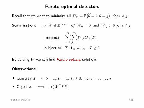
Pareto-optimal detectors
Recall that we want to minimize all Dij = P(θ = i | θ = j
), for i = j
Scalarization: Fix W ∈ Rm×m w/ Wii = 0, and Wij > 0 for i = j
minimizeT
m∑
i=1
m∑
j=1WijDij(T )
subject to T ⊤1m = 1n , T ≥ 0
By varying W we can find Pareto optimal solutions
Observations:
• Constraints ⇐⇒ 1⊤mti = 1, ti ≥ 0, for i = 1, . . . , n
• Objective ⇐⇒ tr(W ⊤TP
)
= tr((WP ⊤)⊤T
)=
∑ni=1 c⊤
i ti
where ci: ith column of C := WP ⊤
Statistical estimation 4-21
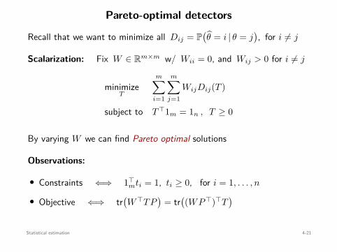
Pareto-optimal detectors
Recall that we want to minimize all Dij = P(θ = i | θ = j
), for i = j
Scalarization: Fix W ∈ Rm×m w/ Wii = 0, and Wij > 0 for i = j
minimizeT
m∑
i=1
m∑
j=1WijDij(T )
subject to T ⊤1m = 1n , T ≥ 0
By varying W we can find Pareto optimal solutions
Observations:
• Constraints ⇐⇒ 1⊤mti = 1, ti ≥ 0, for i = 1, . . . , n
• Objective ⇐⇒ tr(W ⊤TP
)= tr
((WP ⊤)⊤T
)
=∑n
i=1 c⊤i ti
where ci: ith column of C := WP ⊤
Statistical estimation 4-21
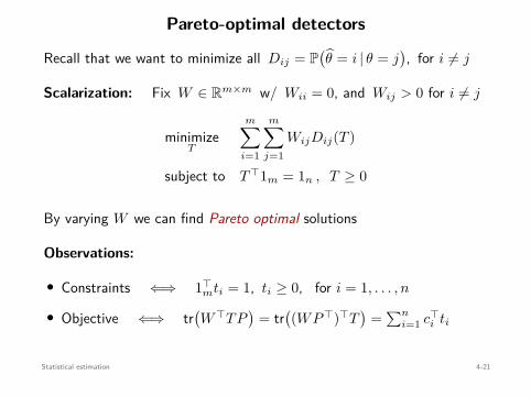
Pareto-optimal detectors
Recall that we want to minimize all Dij = P(θ = i | θ = j
), for i = j
Scalarization: Fix W ∈ Rm×m w/ Wii = 0, and Wij > 0 for i = j
minimizeT
m∑
i=1
m∑
j=1WijDij(T )
subject to T ⊤1m = 1n , T ≥ 0
By varying W we can find Pareto optimal solutions
Observations:
• Constraints ⇐⇒ 1⊤mti = 1, ti ≥ 0, for i = 1, . . . , n
• Objective ⇐⇒ tr(W ⊤TP
)= tr
((WP ⊤)⊤T
)=
∑ni=1 c⊤
i ti
where ci: ith column of C := WP ⊤
Statistical estimation 4-21
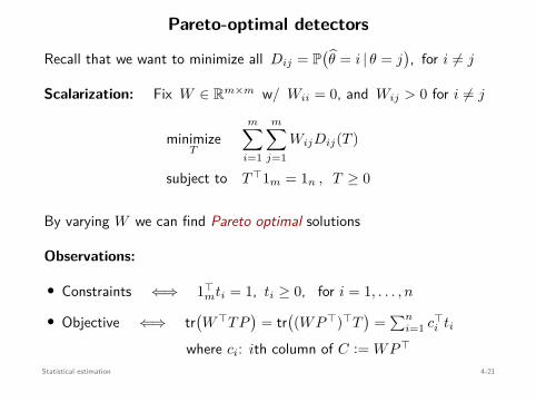
Pareto-optimal detectors
Recall that we want to minimize all Dij = P(θ = i | θ = j
), for i = j
Scalarization: Fix W ∈ Rm×m w/ Wii = 0, and Wij > 0 for i = j
minimizeT
m∑
i=1
m∑
j=1WijDij(T )
subject to T ⊤1m = 1n , T ≥ 0
By varying W we can find Pareto optimal solutions
Observations:
• Constraints ⇐⇒ 1⊤mti = 1, ti ≥ 0, for i = 1, . . . , n
• Objective ⇐⇒ tr(W ⊤TP
)= tr
((WP ⊤)⊤T
)=
∑ni=1 c⊤
i ti
where ci: ith column of C := WP ⊤
Statistical estimation 4-21
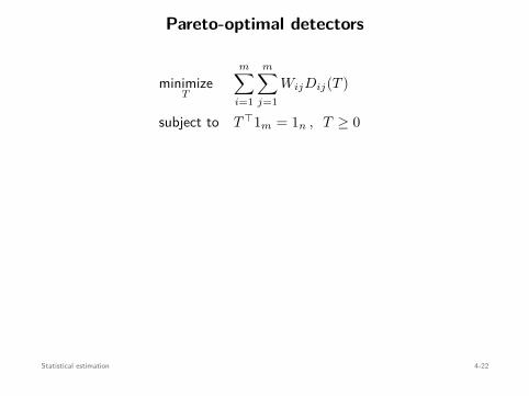
Pareto-optimal detectors
minimizeT
m∑
i=1
m∑
j=1WijDij(T )
subject to T ⊤1m = 1n , T ≥ 0
⇐⇒ minimizet1,...,tn
∑ni=1 c⊤
i ti
subject to 1⊤mti = 1 , ti ≥ 0 , i = 1, . . . , n
Decouples into n independent optimization problems: for column i,
minimizeti
c⊤i ti
subject to 1⊤mti = 1 , ti ≥ 0
t⋆i = (0, . . . , 1, . . . , 0) =⇒ T is deterministic
Rm
−cb
t⋆i
Statistical estimation 4-22
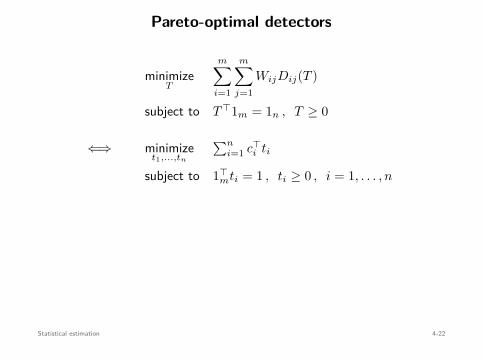
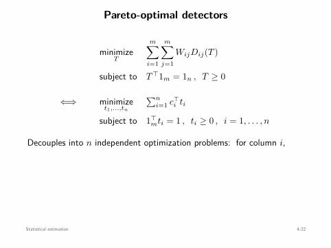
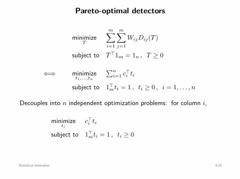
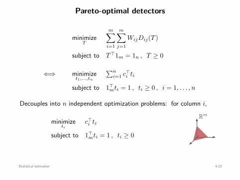
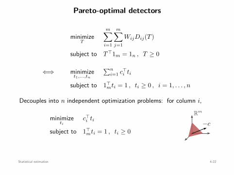
Pareto-optimal detectors
minimizeT
m∑
i=1
m∑
j=1WijDij(T )
subject to T ⊤1m = 1n , T ≥ 0
⇐⇒ minimizet1,...,tn
∑ni=1 c⊤
i ti
subject to 1⊤mti = 1 , ti ≥ 0 , i = 1, . . . , n
Decouples into n independent optimization problems: for column i,
minimizeti
c⊤i ti
subject to 1⊤mti = 1 , ti ≥ 0
t⋆i = (0, . . . , 1, . . . , 0) =⇒ T is deterministic
Rm
−c
b
t⋆i
Statistical estimation 4-22
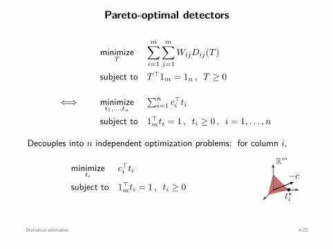
Pareto-optimal detectors
minimizeT
m∑
i=1
m∑
j=1WijDij(T )
subject to T ⊤1m = 1n , T ≥ 0
⇐⇒ minimizet1,...,tn
∑ni=1 c⊤
i ti
subject to 1⊤mti = 1 , ti ≥ 0 , i = 1, . . . , n
Decouples into n independent optimization problems: for column i,
minimizeti
c⊤i ti
subject to 1⊤mti = 1 , ti ≥ 0
t⋆i = (0, . . . , 1, . . . , 0) =⇒ T is deterministic
Rm
−cb
t⋆i
Statistical estimation 4-22
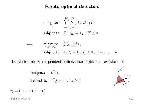
Pareto-optimal detectors
minimizeT
m∑
i=1
m∑
j=1WijDij(T )
subject to T ⊤1m = 1n , T ≥ 0
⇐⇒ minimizet1,...,tn
∑ni=1 c⊤
i ti
subject to 1⊤mti = 1 , ti ≥ 0 , i = 1, . . . , n
Decouples into n independent optimization problems: for column i,
minimizeti
c⊤i ti
subject to 1⊤mti = 1 , ti ≥ 0
t⋆i = (0, . . . , 1, . . . , 0)
=⇒ T is deterministic
Rm
−cb
t⋆i
Statistical estimation 4-22
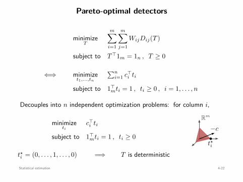
Pareto-optimal detectors
minimizeT
m∑
i=1
m∑
j=1WijDij(T )
subject to T ⊤1m = 1n , T ≥ 0
⇐⇒ minimizet1,...,tn
∑ni=1 c⊤
i ti
subject to 1⊤mti = 1 , ti ≥ 0 , i = 1, . . . , n
Decouples into n independent optimization problems: for column i,
minimizeti
c⊤i ti
subject to 1⊤mti = 1 , ti ≥ 0
t⋆i = (0, . . . , 1, . . . , 0) =⇒ T is deterministic
Rm
−cb
t⋆i
Statistical estimation 4-22
Example: binary hypothesis testing
X is generated by either p1 (θ = 1) or p2 (θ = 2)
P =
P(X = 1 | θ = 1) P(X = 1 | θ = 2)
P(X = 2 | θ = 1) P(X = 2 | θ = 2)...
...P(X = n | θ = 1) P(X = n | θ = 2)
∈ Rn×2
T =
P(θ = 1 | X = 1) P(θ = 1 | X = 2) · · · P(θ = 1 | X = n)
P(θ = 2 | X = 1) P(θ = 2 | X = 2) · · · P(θ = 2 | X = n)
∈ R2×n
D =
P
(θ = 1 | θ = 1
)P
(θ = 1 | θ = 2
)
P(θ = 2 | θ = 1
)P
(θ = 2 | θ = 2
)
=
1 − Pfp Pfn
Pfp 1 − Pfn
Statistical estimation 4-23
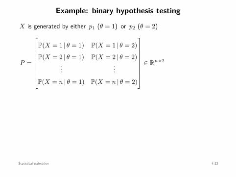
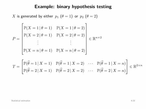
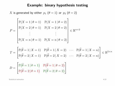
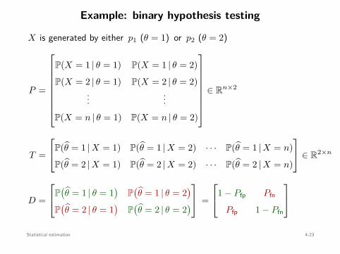
Pareto-optimal detectors:
Select W ∈ R2×2, set C = WP ⊤, and column i of TPO solves
minimizeti
c⊤i ti (ci: column i of C)
subject to 1⊤2 ti = 1 , ti ≥ 0
C =
0 W12
W21 0
P(X = 1 | θ = 1) · · · P(X = n | θ = 1)
P(X = 1 | θ = 2) · · · P(X = n | θ = 2)
=
W12 P(X = 1 | θ = 2) · · · W12 P(X = n | θ = 2)
W21 P(X = 1 | θ = 1) · · · W21 P(X = n | θ = 1)
Therefore,
c⊤i ti = t1i W12 P(X = i | θ = 2) + t2i W21 P(X = i | θ = 1)
Statistical estimation 4-24
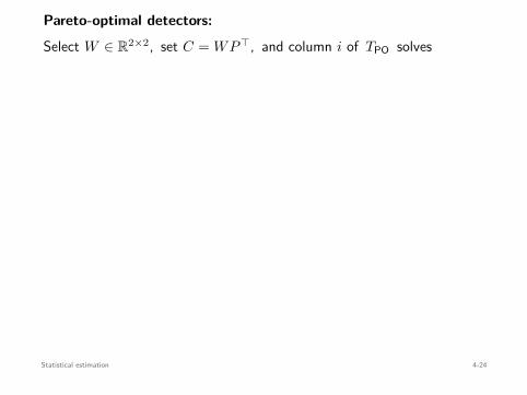
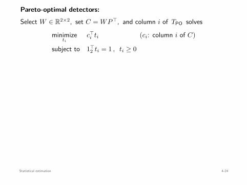
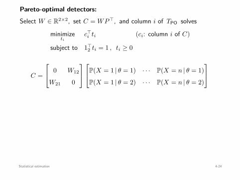
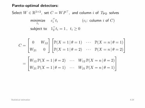
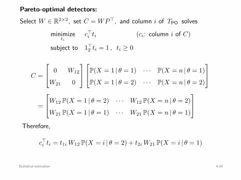
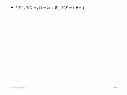
• If W12 P(X = i | θ = 2) < W21 P(X = i | θ = 1),
(t⋆1i , t⋆
2i) = (1 , 0) =⇒ θPO = 1
• If W12 P(X = i | θ = 2) ≥ W21 P(X = i | θ = 1) ,
(t⋆1i , t⋆
2i) = (0 , 1) =⇒ θPO = 2
This is the likelihood-ratio test: Decide θ = 2 if
P(X = i | θ = 2)P(X = i | θ = 1) ≥ W21
W12=: α
Neyman-Pearson lemma:
For each α > 0, the likelihood-ratio test yields a (deterministic)Pareto-optimal detector.
Statistical estimation 4-25
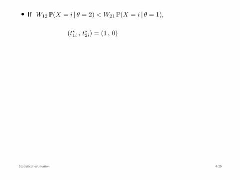
• If W12 P(X = i | θ = 2) < W21 P(X = i | θ = 1),
(t⋆1i , t⋆
2i) = (1 , 0)
=⇒ θPO = 1
• If W12 P(X = i | θ = 2) ≥ W21 P(X = i | θ = 1) ,
(t⋆1i , t⋆
2i) = (0 , 1) =⇒ θPO = 2
This is the likelihood-ratio test: Decide θ = 2 if
P(X = i | θ = 2)P(X = i | θ = 1) ≥ W21
W12=: α
Neyman-Pearson lemma:
For each α > 0, the likelihood-ratio test yields a (deterministic)Pareto-optimal detector.
Statistical estimation 4-25
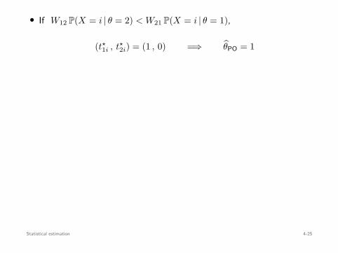
• If W12 P(X = i | θ = 2) < W21 P(X = i | θ = 1),
(t⋆1i , t⋆
2i) = (1 , 0) =⇒ θPO = 1
• If W12 P(X = i | θ = 2) ≥ W21 P(X = i | θ = 1) ,
(t⋆1i , t⋆
2i) = (0 , 1) =⇒ θPO = 2
This is the likelihood-ratio test: Decide θ = 2 if
P(X = i | θ = 2)P(X = i | θ = 1) ≥ W21
W12=: α
Neyman-Pearson lemma:
For each α > 0, the likelihood-ratio test yields a (deterministic)Pareto-optimal detector.
Statistical estimation 4-25
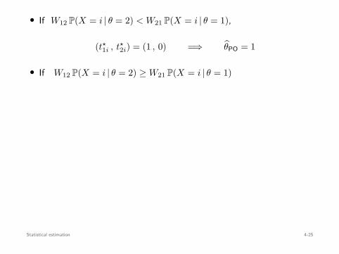
• If W12 P(X = i | θ = 2) < W21 P(X = i | θ = 1),
(t⋆1i , t⋆
2i) = (1 , 0) =⇒ θPO = 1
• If W12 P(X = i | θ = 2) ≥ W21 P(X = i | θ = 1)
,
(t⋆1i , t⋆
2i) = (0 , 1) =⇒ θPO = 2
This is the likelihood-ratio test: Decide θ = 2 if
P(X = i | θ = 2)P(X = i | θ = 1) ≥ W21
W12=: α
Neyman-Pearson lemma:
For each α > 0, the likelihood-ratio test yields a (deterministic)Pareto-optimal detector.
Statistical estimation 4-25
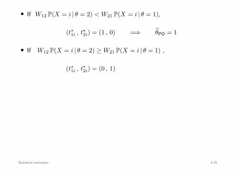
• If W12 P(X = i | θ = 2) < W21 P(X = i | θ = 1),
(t⋆1i , t⋆
2i) = (1 , 0) =⇒ θPO = 1
• If W12 P(X = i | θ = 2) ≥ W21 P(X = i | θ = 1) ,
(t⋆1i , t⋆
2i) = (0 , 1)
=⇒ θPO = 2
This is the likelihood-ratio test: Decide θ = 2 if
P(X = i | θ = 2)P(X = i | θ = 1) ≥ W21
W12=: α
Neyman-Pearson lemma:
For each α > 0, the likelihood-ratio test yields a (deterministic)Pareto-optimal detector.
Statistical estimation 4-25
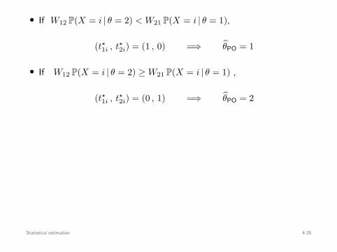
• If W12 P(X = i | θ = 2) < W21 P(X = i | θ = 1),
(t⋆1i , t⋆
2i) = (1 , 0) =⇒ θPO = 1
• If W12 P(X = i | θ = 2) ≥ W21 P(X = i | θ = 1) ,
(t⋆1i , t⋆
2i) = (0 , 1) =⇒ θPO = 2
This is the likelihood-ratio test: Decide θ = 2 if
P(X = i | θ = 2)P(X = i | θ = 1) ≥ W21
W12=: α
Neyman-Pearson lemma:
For each α > 0, the likelihood-ratio test yields a (deterministic)Pareto-optimal detector.
Statistical estimation 4-25
• If W12 P(X = i | θ = 2) < W21 P(X = i | θ = 1),
(t⋆1i , t⋆
2i) = (1 , 0) =⇒ θPO = 1
• If W12 P(X = i | θ = 2) ≥ W21 P(X = i | θ = 1) ,
(t⋆1i , t⋆
2i) = (0 , 1) =⇒ θPO = 2
This is the likelihood-ratio test:
Decide θ = 2 if
P(X = i | θ = 2)P(X = i | θ = 1) ≥ W21
W12=: α
Neyman-Pearson lemma:
For each α > 0, the likelihood-ratio test yields a (deterministic)Pareto-optimal detector.
Statistical estimation 4-25
• If W12 P(X = i | θ = 2) < W21 P(X = i | θ = 1),
(t⋆1i , t⋆
2i) = (1 , 0) =⇒ θPO = 1
• If W12 P(X = i | θ = 2) ≥ W21 P(X = i | θ = 1) ,
(t⋆1i , t⋆
2i) = (0 , 1) =⇒ θPO = 2
This is the likelihood-ratio test: Decide θ = 2 if
P(X = i | θ = 2)P(X = i | θ = 1) ≥ W21
W12=: α
Neyman-Pearson lemma:
For each α > 0, the likelihood-ratio test yields a (deterministic)Pareto-optimal detector.
Statistical estimation 4-25
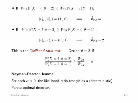
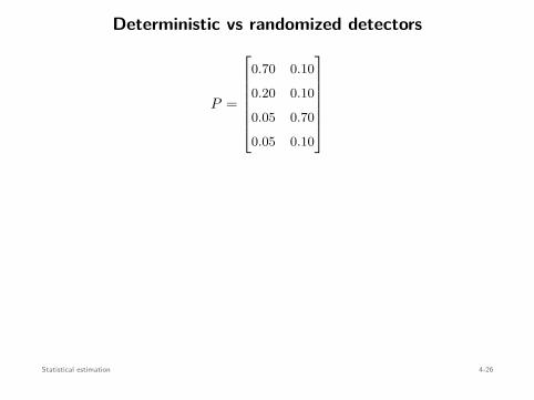
Deterministic vs randomized detectors
P =
0.70 0.10
0.20 0.10
0.05 0.70
0.05 0.10
Varying α yields 3 different Pareto-optimal detectors (excl. extremes):
T(1)PO =
1 0 0 0
0 1 1 1
T
(2)PO =
1 1 0 0
0 0 1 1
T
(3)PO =
1 1 0 1
0 0 1 0
Minimax detector (random):
TMM =
1 2/3 0 0
0 1/3 1 1
Statistical estimation 4-26
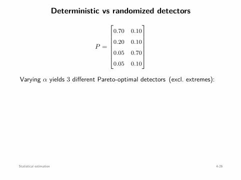
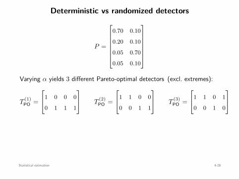
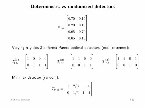
Deterministic vs randomized detectorsReceiver operating characteristic (ROC)
Minimax estimator has (Pfp, Pfn) = ( 16 , 1
6 ) and outperforms anydeterministic estimator
Statistical estimation 4-27
Deterministic vs randomized detectorsReceiver operating characteristic (ROC)
Pfp
Pfn
Minimax estimator has (Pfp, Pfn) = ( 16 , 1
6 ) and outperforms anydeterministic estimator
Statistical estimation 4-27
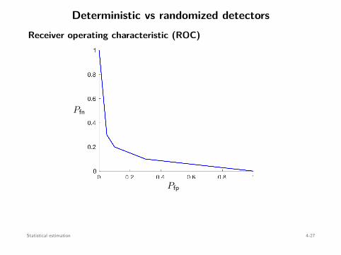
Deterministic vs randomized detectorsReceiver operating characteristic (ROC)
Pfp
Pfn
Minimax estimator has (Pfp, Pfn) = ( 16 , 1
6 ) and outperforms anydeterministic estimator
Statistical estimation 4-27
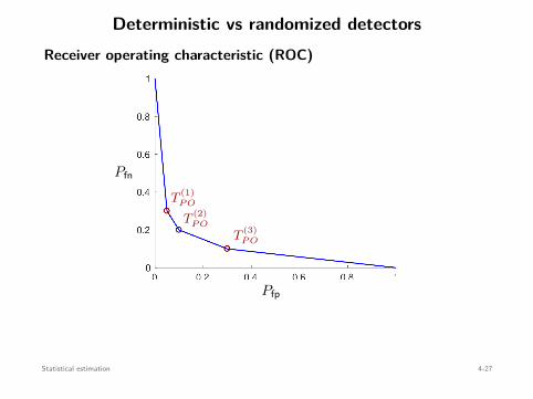
Deterministic vs randomized detectorsReceiver operating characteristic (ROC)
Pfp
Pfn
T(1)P O
T(2)P O
T(3)P O
Minimax estimator has (Pfp, Pfn) = ( 16 , 1
6 ) and outperforms anydeterministic estimator
Statistical estimation 4-27
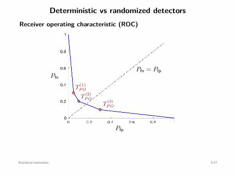
Deterministic vs randomized detectorsReceiver operating characteristic (ROC)
Pfp
Pfn
T(1)P O
T(2)P O
T(3)P O
Pfn = Pfp
Minimax estimator has (Pfp, Pfn) = ( 16 , 1
6 ) and outperforms anydeterministic estimator
Statistical estimation 4-27
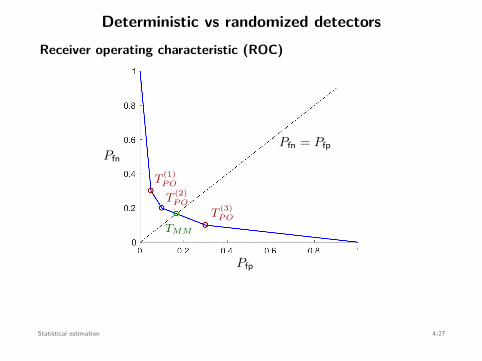
Deterministic vs randomized detectorsReceiver operating characteristic (ROC)
Pfp
Pfn
T(1)P O
T(2)P O
T(3)P O
Pfn = Pfp
TMM
Minimax estimator has (Pfp, Pfn) = ( 16 , 1
6 ) and outperforms anydeterministic estimator
Statistical estimation 4-27
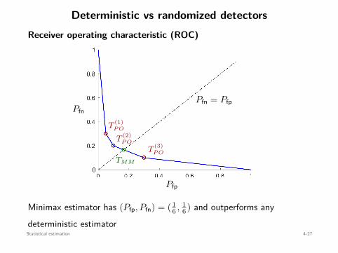
Deterministic vs randomized detectorsReceiver operating characteristic (ROC)
Pfp
Pfn
T(1)P O
T(2)P O
T(3)P O
Pfn = Pfp
TMM
Minimax estimator has (Pfp, Pfn) = ( 16 , 1
6 ) and outperforms anydeterministic estimator
Statistical estimation 4-27

Conclusions
1 2
34
5
6
7
89
x x
convex nonconvex
• Optimization problems arise in many areas
• Essential to distinguish easy (convex) from hard (nonconvex) probs
• Use CVX/CVXPY/Convex for small-scale problems
• Didn’t cover optimality conditions & theory
• Didn’t cover optimization algorithms
• Statistical estimation:Find parameters of distributions (ML/MAP)Entire distributions (nonparametric)
• Multiple hypothesis testing via optimization
Statistical estimation 4-28
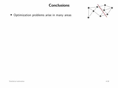
Conclusions1 2
34
5
6
7
89
x x
convex nonconvex
• Optimization problems arise in many areas
• Essential to distinguish easy (convex) from hard (nonconvex) probs
• Use CVX/CVXPY/Convex for small-scale problems
• Didn’t cover optimality conditions & theory
• Didn’t cover optimization algorithms
• Statistical estimation:Find parameters of distributions (ML/MAP)Entire distributions (nonparametric)
• Multiple hypothesis testing via optimization
Statistical estimation 4-28
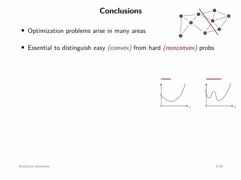
Conclusions1 2
34
5
6
7
89
x x
convex nonconvex
• Optimization problems arise in many areas
• Essential to distinguish easy (convex) from hard (nonconvex) probs
• Use CVX/CVXPY/Convex for small-scale problems
• Didn’t cover optimality conditions & theory
• Didn’t cover optimization algorithms
• Statistical estimation:Find parameters of distributions (ML/MAP)Entire distributions (nonparametric)
• Multiple hypothesis testing via optimization
Statistical estimation 4-28
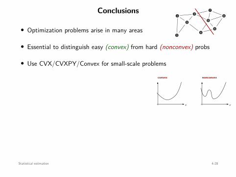
Conclusions1 2
34
5
6
7
89
x x
convex nonconvex
• Optimization problems arise in many areas
• Essential to distinguish easy (convex) from hard (nonconvex) probs
• Use CVX/CVXPY/Convex for small-scale problems
• Didn’t cover optimality conditions & theory
• Didn’t cover optimization algorithms
• Statistical estimation:Find parameters of distributions (ML/MAP)Entire distributions (nonparametric)
• Multiple hypothesis testing via optimization
Statistical estimation 4-28
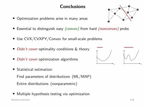
Conclusions1 2
34
5
6
7
89
x x
convex nonconvex
• Optimization problems arise in many areas
• Essential to distinguish easy (convex) from hard (nonconvex) probs
• Use CVX/CVXPY/Convex for small-scale problems
• Didn’t cover optimality conditions & theory
• Didn’t cover optimization algorithms
• Statistical estimation:Find parameters of distributions (ML/MAP)Entire distributions (nonparametric)
• Multiple hypothesis testing via optimizationStatistical estimation 4-28

References and Resources
Lectures:
• web.stanford.edu/∼boyd/cvxbook/
• users.isr.ist.utl.pt/∼jxavier/NonlinearOptimization18799-2018
• www.seas.ucla.edu/∼vandenbe/ee236cStatistical estimation 4-29