Embed Size (px)
Citation preview

Fundamentals of Media Processing
Lecturer:
池畑 諭(Prof. IKEHATA Satoshi)児玉 和也(Prof. KODAMA
Kazuya)
Support:
佐藤 真一(Prof. SATO Shinichi)孟 洋(Prof. MO Hiroshi)

Course Overview (15 classes in total)
1-10 Machine Learning by Prof. Satoshi Ikehata
11-15 Signal Processing by Prof. Kazuya Kodama
Grading will be based on the final report.

10/16 (Today) Introduction
10/23 Basic mathematics (1) (Linear algebra, probability, numerical computation)
10/30 Basic mathematics (2) (Linear algebra, probability, numerical computation)
11/6 Machine Learning Basics (1)
11/20 Deep Feedforward Networks
11/27 Regularization and Deep Learning
12/4 Optimization for Training Deep Models
12/11 Convolutional Neural Networks and Its Application (1)
12/18 Convolutional Neural Networks and Its Application (2)
11/13 Machine Learning Basics (2)
Basic of Machine Learning (Maybe for beginners)
Basic of Deep Learning
CNN and its Application
Chap. 2,3,4
Chap. 2,3,4
Chap. 1
Chap. 5
Chap. 5
Chap. 6
Chap. 7
Chap. 8
Chap. 9 and more
Chap. 9 and more

Convolutional Neural Networks

History of Convolutional Neural Networks
◼ 1990s, the neural network research group at AT & T developed
a convolutional network for reading checks (LeCun1998)
◼ Several OCR and handwriting recognition systems based on
CNN were deployed by Microsoft (Simard2003)
◼ AlexNet (2012) won the ImageNet object recognition
challenge, and the current intensity of commercial interest in
deep learning began
0
20
40
60
80
100
120
140
2010 2011 2012 2013 2014 2015 2016 2017 2018
# of Papers with “Deep” in CVPR

https://cdn-images-1.medium.com/max/1600/1*ZCjPUFrB6eHPRi4eyP6aaA.gif
Convolutional Neural Networks (1)
◼ Convolutional Neural networks (CNN; LeCun1989) are a neural
network for processing data of gild-like structure. The major
examples include image data
◼ CNN are simply neural networks that use convolution in piece of
general matrix multiplication in at least one of their layers. In
general convolution, the kernel is flipped, but in neural networks,
it does not matter since the kernel itself is learned
𝑆 𝑖, 𝑗 = 𝐼 ∗ 𝐾 𝑖, 𝑗 =
𝑚
𝑛
𝐼 𝑖 + 𝑚, 𝑖 + 𝑛 𝐾(𝑖, 𝑗)
Cross correlation based on the
commutative property in convolution
◼ The multichannel convolutional operations requires that the input
and output of the convolution have same channels to make the
convolution commutative; In reality, what CNN do is cross
correlation rather than convolution

◼ CNN leverages three important ideas
⚫ Sparse interactions
- Each unit is interacted with smaller number of units
⚫ Parameter sharing
- Traditional neural net→ dense multiplication (𝑦 = 𝑊𝒙)
- We only need few parameters (# of kernel × size of kernel)
⚫ Equivariant to translation
- 𝑓 𝑔 𝑥 = 𝑔(𝑓(𝑥))
- “translation then convolution” is same with “convolution,
then translation”
- CNN is not naturally equivalent to rotation and scale
CNNStandard NN
Convolutional Neural Networks (2)

Convolutional Neural Networks (3)

CNN and Neuroscience (1)
https://www.researchgate.net/figure/Schematic-diagram-of-anatomical-connections-and-neuronal-selectivities-of-early-visual_fig15_268228820
https://www.intechopen.com/books/visual-cortex-current-status-and-perspectives/adaptation-and-neuronal-network-in-visual-cortex

CNN and Neuroscience (2)
◼ V1 cells have weights that are described by Gabor functions that
prefers the specific direction of edges
Feature maps learned by CNN

Example of the CNN
◼ Convolutional neural networks consist of convolution,
pooling, and fully-connected layers

Pooling (1)
◼ A pooling function replaces the output of the net at a certain
location with a summary statistic of the nearby outputs
⚫ Max pooling: the maximum within a rectangular neighborhood
⚫ Average pooling: the mean within a rectangular neighborhood
12 20 30 0
8 12 2 0
34 70 37 4
112 100 25 12
20
112
30
37
13
79
8
20
Max pooling Average pooling
◼ Pooling encourages the network to learn the invariance to small
translations of the input
◼ For many tasks, pooling is essential for handling inputs of varying
size (varying the size of an offset between pooling regions so that
the final output layer always receives the same number of
summary statistics regardless of the input size)

Pooling (2)
◼ Boureau2010 (mentioned in image classification task):
“Depending on the data and features, either max or average pooling
may perform best. The optimal pooling type for a given classification
problem may be neither max nor average pooling”
Average Max

◼ An infinitely strong prior places zero probability on some
parameters and says these parameter values are completely
forbidden. We can imagine CNN as being similar to a fully
connected net but with an infinitely strong prior over its weights
(e.g., translation invariance) and without some priors in standard
neural network (e.g., permutation invariance)
◼ Convolution and pooling can cause underfitting. If a task relies
on preserving precise spatial information, then using pooling
on all features can increase the training error. Some CNN
therefore uses pooling on some specific channels
(Szegedy2014) in order to get both highly invariant features
and features that will not underfit when the translation
invariance prior is incorrect
Pooling (3)

Variance of the Basic Convolution Function (1)
◼ The convolution function used in CNN and the standard discrete
convolution operation is usually different
• The convolution in CNN is an operation that consists of
many applications of convolution in parallel to extract many
kinds of features at many locations
• The input and output are grid of vector-valued observations
(i.e., 3-D tensors; e.g., RGB image)
◼ Stride: We may want to skip over some positions of the kernel
to reduce the computational cost. We can define a downsampled
convolution function with stride as:
𝑍𝑖,𝑗,𝑘 =
𝑙,𝑚,𝑛
𝑉𝑙,𝑗+𝑚−1,𝑘+𝑛−1𝐾𝑖,𝑙,𝑚,𝑛𝑖: output channel
𝑙: input channel
𝑍𝑖,𝑗,𝑘 =
𝑙,𝑚,𝑛
𝑉𝑙, 𝑗−1 ∗𝑠+𝑚, 𝑘−1 ∗𝑠+𝑛𝐾𝑖,𝑙,𝑚,𝑛Downsampled convolution
with stride (s)
𝑗: offset of rows
𝑘: offset of columns

Variance of the Basic Convolution Function (2)
◼ To avoid shrink of the output size after the convolution, we can
do zero padding of the input V to make it wider
• valid convolution: The output size shrinks
• same convolution: The output size is same with the input
◼ Tiled convolution (Gregor2010): offers a compromise between
a convolutional layer and a locally connected layer (learning a
separate set of weights at every spatial location to emphasize the
local information). We learn a set of kernels that we rotate
through as we move through space, which implies that we use
different kernels at different locations.
◼ To back-propagate the convolution layer, we can simply see the
convolution operation as a (sparse) matrix multiplication. As for
the bias, it is typical to have one bias per channel of the output
and share it across all locations (for tiled convolution, across
same tiling patterns as the kernels)

Learning A Simple Convolutional Neural Networks
◼ Suppose we want to train a convolutional network that
incorporates strided convolution of kernel stack 𝐾 applied to
multichannel image 𝑉 with stride s
◼ Suppose the loss function is 𝐽(𝑉, 𝐾). • During the back propagation, we will receive a tensor G
such that
• To train the network we need to compute the derivatives
with respect to the weights in the kernel:
• We may need to compute the gradient with respect to the
hidden layer V,
𝜕
𝜕𝐾𝑖,𝑗,𝑘,𝑙𝐽 𝑉, 𝐾 =
𝑚,𝑛
𝐺𝑖,𝑚,𝑛𝑉𝑗, 𝑚−1 ∗𝑠+𝑘, 𝑛−1 ∗𝑠+𝑙
𝐺𝑖,𝑗,𝑘 =𝜕
𝜕𝑍𝑖,𝑗,𝑘𝐽(𝑉, 𝐾) (Z is the output of the convolution).
𝜕
𝜕𝑉𝑖,𝑗,𝑘𝐽 𝑉, 𝐾 =
𝑙,𝑚 (s.t. 𝑙−1 ∗𝑠+𝑚=𝑗)
𝑛,𝑝 (s.t. 𝑛−1 ∗𝑠+𝑝=𝑘
𝐾𝑞,𝑖,𝑚,𝑝𝐺𝑞,𝑙,𝑛

Structured Outputs
◼ Convolutional networks can be used to output a high-
dimensional structured object (e.g., semantic segmentation)
◼ The issue is the output dimension can be smaller then input due to
the pooling layers with large stride. To overcome this issue:
a. Produce an initial guess at low resolution, then refine it using
graphical model such as CRF/MRF
b. Use upsampling/unpooling layer to increase the output size

Data Types
◼ One advantage to fully-convolutional neural networks is that
they can process inputs with varying size of images in
training/test data (note that valid for only spatial variation)
◼ If we put the dense layer with convolution layer (e.g., for
assigning label to an entire image), we need some additional
design steps, like inserting a pooling layer whose pooling
regions scale in size proportional to the size of the input to
maintain a fixed number of pooled outputs
Long et al., “Fully convolutional networks for semantic segmentation”, In CVPR2015


Random and Unsupervised Features
◼ The forward/backward propagation for the supervised training
of CNN is time consuming. One way to reduce the cost of
convolutional neural network training is to use features that are
not trained in a supervised fashion
◼ One is to initialize them randomly (e.g., Jarrett2009), another is
to design them by hand (e.g., edge detector). Finally, one can
learn the kernels with an unsupervised criterion (e.g.,
Coates2011 applied k-means clustering to small image patches
then use each learned centroid as convolution kernel)
◼ A greedy layer-wise pretraining (e.g., Lee2009) train the first
layer in isolation, then extract all features from the first layer
only once then train the second layer in isolation and so on.
◼ Today, it is common to learn the CNN in purely supervised manner

Preprocessing
◼ In computer vision applications, images should be standardized so
that their pixels all lie in the same reasonable range (e.g., [0,1]).
Mixing different ranges results in failure. The common procedure
is to subtract the mean from each image and divide it by std (global
contrast normalization) or do it per local region (local contrast
normalization). The result is the image of zero-mean and one-std
◼ The images should have the same aspect ratio (generally square)
achieved by clopping and scaling

Design of the Hyperparameters in CNN

Applications of CNN

Image Classification
◼ ImageNet Large Scale Visual Recognition Competition
(ILSVRC): 1.2M for training, 150K for test.
◼ Object localization for 1000 categories, object detection for 200
categories, object detection from video for 30 categories

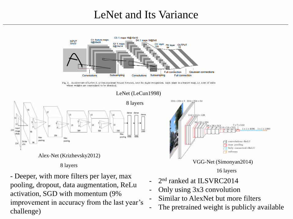
LeNet and Its Variance
Alex-Net (Krizhevsky2012)
VGG-Net (Simonyan2014)8 layers
16 layers
LeNet (LeCun1998)
8 layers
- Deeper, with more filters per layer, max
pooling, dropout, data augmentation, ReLu
activation, SGD with momentum (9%
improvement in accuracy from the last year’s
challenge)
- 2nd ranked at ILSVRC2014
- Only using 3x3 convolution
- Similar to AlexNet but more filters
- The pretrained weight is publicly available

GoogLeNet and Inception Module
◼ Google-Net (Segedy2014): Won ILSVRC2014 (22 Layers)
◼ 1x1 convolution is used as a dimension reduction
https://medium.com/coinmonks/paper-review-of-googlenet-inception-v1-winner-of-ilsvlc-2014-image-classification-c2b3565a64e7
Inception module
◼ Global average pooling is introduced by averaging feature map
from 7x7 to 1x1 to remove the weights for FCN layers

Deep Residual Networks
◼ ResNet (He2015): Won ILSVRC2015 (152 layers)
◼ Basic concept is “More Layers is Better”
◼ To avoid vanishing gradient problem, the residual function
𝐻 𝑥 = 𝐹 𝑥 + 𝑥 is introduced which allows the gradient being
rapidly propagated through the network when applying backprop

1x1 1x1 1x1
Densely Connected Convolutional Networks
◼ DenseNets (Huang2017): introduces direct connections between
any two layers with the same feature-map size. The idea behind is
“it may be useful to reference feature maps from earlier in the
network”
◼ DenseNets require substantially fewer parameters and less
computation to achieve state-of-the-art performance

Object Detection (1)
◼ Object detection task in the context of deep neural networks asks
“where the object is” as well as “what is the object”
From Liu2014

Object Detection (2)
◼ Regions with Convolutional Neural Networks (R-CNN;
Girshick2013): (a) extract region proposals (b) where CNN is
applied for extracting features, (c) which are then classified using
SVM, (d) then bounding box regression is applied
◼ The original R-CNN introduces selective search (hierarchical
grouping) for region extraction: (a) initial candidate regions, (b)
use greedy algorithm to merge similar regions into larger one
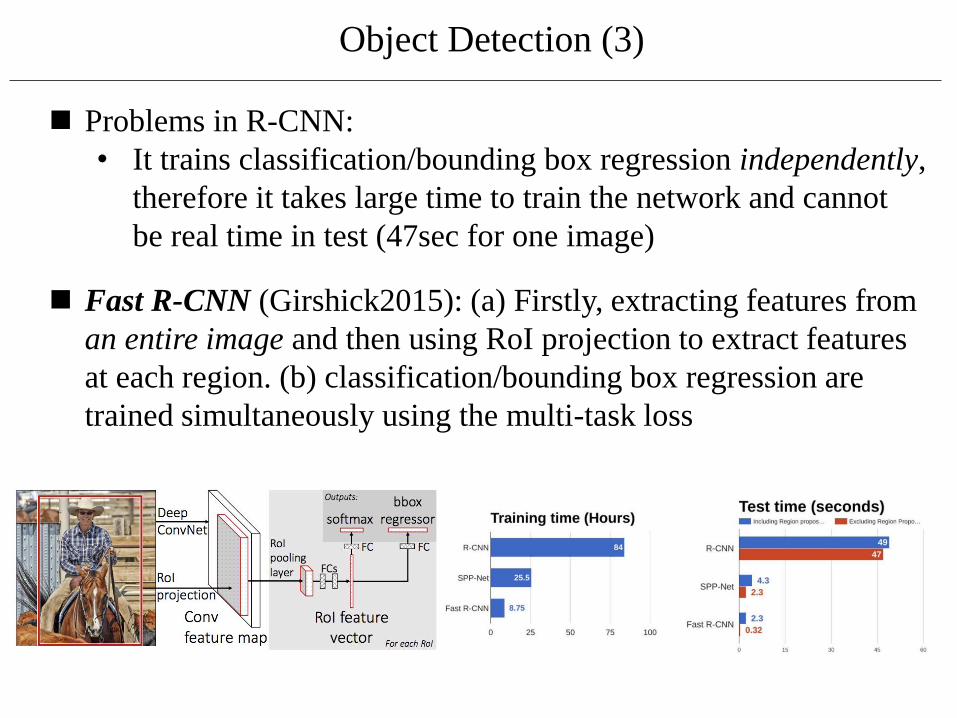
Object Detection (3)
◼ Fast R-CNN (Girshick2015): (a) Firstly, extracting features from
an entire image and then using RoI projection to extract features
at each region. (b) classification/bounding box regression are
trained simultaneously using the multi-task loss
◼ Problems in R-CNN:
• It trains classification/bounding box regression independently,
therefore it takes large time to train the network and cannot
be real time in test (47sec for one image)
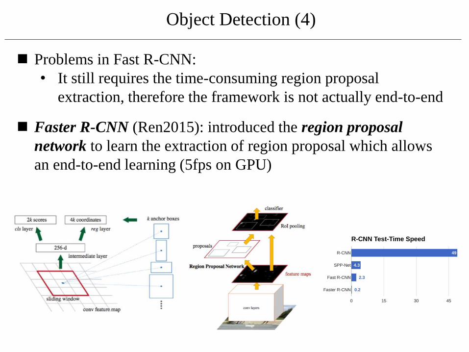
Object Detection (4)
◼ Faster R-CNN (Ren2015): introduced the region proposal
network to learn the extraction of region proposal which allows
an end-to-end learning (5fps on GPU)
◼ Problems in Fast R-CNN:
• It still requires the time-consuming region proposal
extraction, therefore the framework is not actually end-to-end

Object detection in the wild by Faster R-CNN + ResNet-101
https://www.youtube.com/watch?v=WZmSMkK9VuA

Object Detection (5)
◼ YOLO (You Only Look Once; Redmon2016): unlike previous
algorithms that are “proposal extraction + classification”, YOLO
uses a single CNN to predicts the bounding boxes and the class
probabilities for the box (use information outside the local region)
◼ YOLO takes an image and split it into grid, within each of the
grid bounding boxes are taken. The bounding boxes whose class
probability is above a threshold is selected to locate the object
◼ 2x faster but less accurate than Faster R-CNN. It is also weak for
small objects

https://www.youtube.com/watch?v=V4P_ptn2FF4

Object Detection (6)
◼ Mask R-CNN (He2017):
• Solved the “subpixel shift”
problem in Faster R-CNN
• Can also predict object masks


Semantic Segmentation (1)
◼ Semantic segmentation task is to predict a pixel-wise instance
label corresponding to an input image or vide frames
◼ VOC2012 and MSCOCO are important benchmark datasets
◼ Unlike other CNN tasks, the output is structured (e.g,. image)
SegNet: https://www.youtube.com/watch?v=CxanE_W46ts

FCN (Long2014)
Semantic Segmentation (2)
◼ The standard strategy is to use the encoder-decoder architecture
DeconvNet (Noh2015)
No skip
connection

Semantic Segmentation (3)
◼ Unpooling: the reverse operation of max pooling. It recodes the
locations of maximum activations selected during pooling operation
in switch variables, which are employed to place each activation
back to its original pooled location
◼ Deconvolution (transposed convolution): densify the sparse
activations obtained by unpooling through convolution-like
operations with multiple learned filters
Deconvolution operation

Seg-Net (Badrinarayanan2015)
Semantic Segmentation (5)
U-Net (Ronneberger2015)
◼ Skip connection is a very powerful tool to keep the original
resolution and propagate loss effectively in back propagation
w/ class balancing
w/ weighted loss on boundary

Semantic Segmentation (6)
◼ Other than the encoder-decoder like net, we can use the dilated
convolution (Yu2015) without using pooling to keep the original
resolution
https://github.com/vdumoulin/conv_arithmetic

https://blog.mapillary.com/update/2018/06/14/robust-cv.html
Semantic Segmentation (7)
◼ One of the current state-of-the-art works (Bulo2018)

Other Important Architectures (1)
◼ Stacked Hourglass Networks (Newell2016) was proposed to
extract multi-scale feature extraction in a single path
◼ SHNet consists of multiple encoder-decoder networks with skip
connections

Other Important Architectures (2)
◼ Deep learning on 3-D data (e.g., voxel, point could) is a challenging
task due to the high-dimensinoality. The main approaches are
categorized into two: (a) 3-D CNN on regular voxels, (b) 3-D CNN
on irregular point cloud (or graph). An example of the latter approach
was given by Su2018 with BCL (bilateral convolution layer)

Other Important Architectures (3)
◼ Stereo matching is an important 3-D vision task to achieve the
autonomous driving car. The input is two or more images instead of
one (in similar with the optical flow estimation)
Kendall, Alex, et al. "End-to-End Learning of Geometry and Context for Deep Stereo Regression,2016

Similar concept in “Yu et al., Deep Stereo Matching with Explicit Cost Aggregation Sub-Architecture, 2018”
Introduced the concept of “Joint Filtering on Cost Volume”
Other Important Architectures (4)
◼ The recent trend is to use the end-to-end stereo regression model:
Cost aggregation part is
incorporated in the architecture

Other Important Architectures (5)
◼ The multi-task training is one of the most interesting topics
Yang et.al., SegStereo: Exploiting Semantic Information for Disparity Estimation, ECCV2018

Zhou et al., Unsupervised Learning of Stereo Matching, ICCV2017
Other Important Architectures (6)
◼ Unsupervised CNN is a new topic to train the network without
training data. The CNN is combined with traditional model-based
approaches to compute the loss (e.g., window-based stereo matching)

Introduction of My Work
Photometric Stereo

INPUT OUTPUT
Photometric Stereo

𝐼 𝑐(𝐼) 𝐼′
RAW Camera
TransformCamera
Image
𝒍
𝒏
𝒗
𝜖
𝑐
𝜌
𝜌
𝒏
𝒍1
BRDF
normallight
Model Error
𝜌
𝜌
𝒗view
⋮
𝒏
𝒍𝟐𝒗
𝒏
𝒍∞𝒗
+
+
Imaged-based 3D Modeling
Geometrical Optical
SLAM, SfM,
Multi-view Stereo
Photometric Stereo (#IMG ≥ 2),
Shape-from-Shading (#IMG = 1),
Inverse Projection Inverse Light Transport

R. J. Woodham, Photometric Method for Determining Surface Orientation from Multiple Images. Optical Engineering 19(1)139–144 (1980).
Surface Plane
Camera
Light 1
Light 2
Light 3
The First Photometric Stereo Algorithm
(Woodham1980)
If following assumptions are held,
Surface normals are uniquely recovered from
images under three different illumination
- Lambertian reflectance
- known directional light sources
- no shadows and ambient(natural) illumination
𝜌(𝒏, 𝒍, 𝒗)
𝒏
𝒍
𝒗
𝐼
BRDF RAW
𝜖normal
light
view
+
Lambertian
Gaussian

A Benchmark Dataset and Evaluation for Non-Lambertian and Uncalibrated Photometric Stereo
Boxin Shi, Zhe Wu, Zhipeng Mo, Dinglong Duan, Sai-Kit Yeung, and Ping Tan In Proc. IEEE Conf. on Computer Vision and Pattern
Recognition (CVPR) Las Vegas, NV, USA, Jun. 2016
Unfortunately, Real Scenes Are NOT Lambertian

Better BRDF (𝜌) Modeling
Bett
er
Err
or
(𝜖)
Modelin
g
+
Wu2010
Ikehata2012, 2017
Woodham1980
Hernández 2010
Ikehata2014
Goldman2010Shi2014
Ikehata2014
Ikehata2018
Wan2017Other classes
BRDF/Error Modeling in Calibrated
Non-Lambertian Photometric Stereo

[1] S. Ikehata, D. Wipf, Y. Matsushita and K. Aizawa, “Robust Photometric Stereo Using Sparse Regression”, CVPR2012
[2] S. Ikehata, D. Wipf, Y. Matsushita and K. Aizawa, “Photometric Stereo using Sparse Bayesian Regression for General Diffuse Surfaces”, IEEE TPAMI, 2014
noiseshadow
Narrow Specular
CVPR2012(*1) TPAMI2014(*2) NIPS2017(*3)
ObservationDiffuse(D)
Error(E)
Maximize the sparsity of the
error matrix
General diffuse
[3] Hao He, Bo Xin, Satoshi Ikehata, David Wipf, “From Sparse Bayesian Learning to Deep Recurrent Nets”, NIPS2017 (Oral)
Lambertian
Sparse Bayesian Learning RCNN
For Better Outlier Handling
Photometric stereo using
sparse regression
Lambertian
L0 minimization
algorithm
Inlier model

For General Isotropic Materials
K-lobe-isotropic-BRDF-based PS[CVPR2014(*1) ]
𝜌 = 𝜌1 𝒏𝑇𝜶1 + 𝜌2 𝒏𝑇𝜶2 +⋯+ 𝜌𝐾(𝒏𝑇𝜶𝐾) (shape const.)
K-lobe isotropic BRDF by Chandarker2013
𝒏𝑇𝒍
𝐼
𝒍𝑇𝒗 𝑙2
𝑙1
𝑙3
𝑔0,0(𝐼, 𝒍𝑇𝒗)
𝑔0,1(𝐼, 𝒍𝑇𝒗)
𝑔1,0(𝐼, 𝒍𝑇𝒗)
𝑔𝑘1,𝑘2(𝐼, 𝒍𝑇𝒗)
𝑔𝐾1,𝐾2(𝐼, 𝒍𝑇𝒗)
𝒏,𝜷
Linearize
・ Non-linear model
・ Non-linear constraints
・ Linear model
・ Linear constraints
[1] S. Ikehata and K. Aizawa, “Photometric Stereo using Constrained Bivariate Regression for Spatially Varying Isotropic Surfaces”, CVPR2014 (Oral)
Solve the dual problem
in a tractable formRendered with MERL BRDF database

A Benchmark Dataset and Evaluation for Non-Lambertian and Uncalibrated Photometric Stereo
Boxin Shi, Zhe Wu, Zhipeng Mo, Dinglong Duan, Sai-Kit Yeung, and Ping Tan In Proc. IEEE Conf. on Computer Vision and Pattern
Recognition (CVPR) Las Vegas, NV, USA, Jun. 2016
Best accuracy in robust approaches
Best accuracy without specular removal
DiLiGenT Benchmark
(Shi2016)
⚫ Photometric stereo image dataset
with calibrated Directional Lightings,
objects of General reflectance, and
ground Truth shapes (normals)
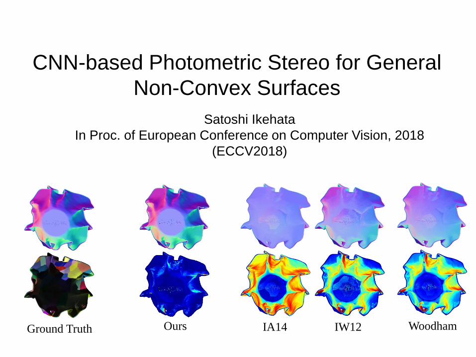
CNN-based Photometric Stereo for General
Non-Convex Surfaces
Satoshi Ikehata
In Proc. of European Conference on Computer Vision, 2018
(ECCV2018)
Ours IA14 IW12 WoodhamGround Truth

◼ Multiple interactions of light and surface are difficult to be modeled in a
mathematically tractable form
Direct
illumination
Direct + indirect
illumination
Convex Nonconvex
Can neural networks represent this complicated interaction?
Photometric Stereo for Non-Convex Surfaces

…
Fixed size input (LR images) Unordered, hundreds of images
(+ lighting direction)
Structured Input Unstructured Input
…?
Two-view stereo Multi-view stereo
CNN CNNInput Input
Photometric stereo
Challenges in PS with Deep Learning

3
3
Target pixel
Target pixel
𝒏𝐺𝑇 𝒏𝐺𝑇
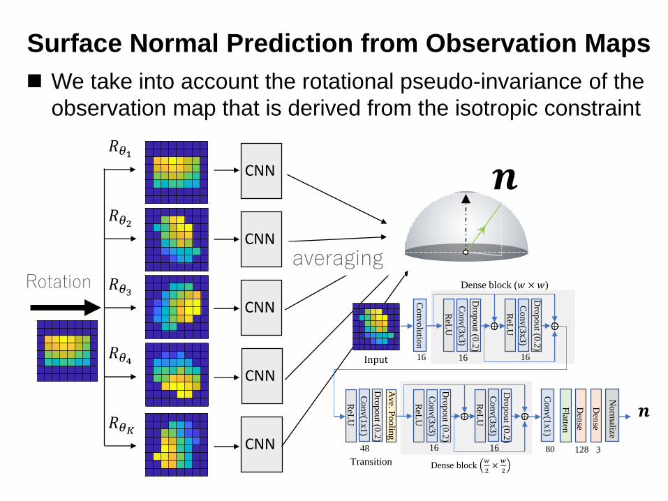
Solution: 2-D Observation map as Input of CNN
◼ All the photometric stereo inputs (images, lights) per pixel are merged
to a fixed-size, intermediate representation called observation map.
An observation map reasonably encodes the geometry, material and
behavior of the light at around a surface point
Projecting observations to a 2-D map based on the light directions
CNN
CNN
CNN
CNN
CNN
𝑅𝜃2
𝑅𝜃1
𝑅𝜃3
𝑅𝜃4
𝑅𝜃𝐾
𝒏
Rotationaveraging
Input
Co
nvo
lutio
n
ReL
U
Dro
po
ut (0
.2)
Co
nv(3
x3
)
ReL
U
Dro
po
ut (0
.2)
Co
nv(3
x3
)
ReL
U
Dro
po
ut (0
.2)
Co
nv(1
x1
)
Co
nv(1
x1
)
Den
se
Den
se
Flatten
No
rmalize
ReL
U
Dro
po
ut (0
.2)
Co
nv(3
x3
)
ReL
U
Dro
po
ut (0
.2)
Co
nv(3
x3
)
Dense block (𝑤 × 𝑤)
Dense block 𝑤
2×
𝑤
2
Ave. P
oo
ling
Transition
16 16 16
48 16 16 80 128 3
𝒏
Surface Normal Prediction from Observation Maps
◼ We take into account the rotational pseudo-invariance of the
observation map that is derived from the isotropic constraint

Rendered image
baseColor
roughness
Render
object
Parameters of
BSDF
Synthetic Dataset for Training Networks

Experimental Results
Ours (K=10) TH18 IW14 ST14GT
HARVEST, 96 lightings
BALL BEAR BUDDHA CAT COW GOBLET HARVEST POT1 POT2 READING AVE. ERR
OURS 2.2 4.1 7.9 4.6 8.0 7.3 14.0 5.4 6.0 12.6 7.2
HS17 [20] 1.3 5.6 8.5 4.9 8.2 7.6 15.8 5.2 6.4 12.1 7.6
TM18 [21] 1.5 5.8 10.4 5.4 6.3 11.5 22.6 6.1 7.8 11.0 8.8
IW14 [7] 2.0 4.8 8.4 5.4 13.3 8.7 18.9 6.9 10.2 12.0 9.0
SS17 [19] 2.0 6.3 12.7 6.5 8.0 11.3 16.9 7.1 7.9 15.5 9.4
ST14 [18] 1.7 6.1 10.6 6.1 13.9 10.1 25.4 6.5 8.8 13.6 10.3
SH17 [25] 2.2 5.3 9.3 5.6 16.8 10.5 24.6 7.3 8.4 13.0 10.3
IA14 [17] 3.3 7.1 10.5 6.7 13.1 9.7 26.0 6.6 8.8 14.2 10.6
GC10 [14] 3.2 6.6 14.9 8.2 9.6 14.2 27.8 8.5 7.9 19.1 12.0
BASELINE [12] 4.1 8.4 14.9 8.4 25.6 18.5 30.6 8.9 14.7 19.8 15.4
Table. Quantitative comparison on DiLiGenT Dataset