Futures Price under the BOPM - 國立臺灣大學lyuu/finance1/2017/20170426.pdf · Martingale Pricing and Numerairea • Themartingalepricingformula(67)onp.518usesthe moneymarketaccountasnumeraire.b

Futures Price under the BOPM

• Futures prices form a martingale under the risk-neutral

probability.

– The expected futures price in the next period isa

pfFu+ (1− pf)Fd = F

(1− d

u− du+

u− 1

u− dd

)= F.

• Can be generalized to

Fi = Eπi [Fk ], i ≤ k,

where Fi is the futures price at time i.

• This equation holds under stochastic interest rates, too.b

aRecall p. 476.bSee Exercise 13.2.11 of the textbook.

c©2017 Prof. Yuh-Dauh Lyuu, National Taiwan University Page 521

Martingale Pricing and Numerairea

• The martingale pricing formula (67) on p. 518 uses the

money market account as numeraire.b

– It expresses the price of any asset relative to the

money market account.

• The money market account is not the only choice for

numeraire.

• Suppose asset S’s value is positive at all times.

aJohn Law (1671–1729), “Money to be qualified for exchaning goods

and for payments need not be certain in its value.”bLeon Walras (1834–1910).


Martingale Pricing and Numeraire (concluded)

• Choose S as numeraire.

• Martingale pricing says there exists a risk-neutral

probability π under which the relative price of any asset

C is a martingale:

C(i)

S(i)= Eπ

i

[C(k)

S(k)

], i ≤ k.

– S(j) denotes the price of S at time j.

• So the discount process remains a martingale.a

aThis result is related to Girsanov’s theorem (1960).


Example

• Take the binomial model with two assets.

• In a period, asset one’s price can go from S to S1 or

S2.

• In a period, asset two’s price can go from P to P1 or

P2.

• Both assets must move up or down at the same time.

• Assume

S1

P1<

S

P<

S2

P2(68)

to rule out arbitrage opportunities.


Example (continued)

• For any derivative security, let C1 be its price at time

one if asset one’s price moves to S1.

• Let C2 be its price at time one if asset one’s price

moves to S2.

• Replicate the derivative by solving

αS1 + βP1 = C1,

αS2 + βP2 = C2,

using α units of asset one and β units of asset two.


Example (continued)

• By Eqs. (68) on p. 524, α and β have unique solutions.

• In fact,

α =P2C1 − P1C2

P2S1 − P1S2and β =

S2C1 − S1C2

S2P1 − S1P2.

• The derivative costs

C = αS + βP

=P2S − PS2

P2S1 − P1S2C1 +

PS1 − P1S

P2S1 − P1S2C2.


Example (continued)

• It is easy to verify that

C

P= p

C1

P1+ (1− p)

C2

P2.

– Above,

pΔ=

(S/P )− (S2/P2)

(S1/P1)− (S2/P2).

– By Eqs. (68) on p. 524, 0 < p < 1.

• C’s price using asset two as numeraire (i.e., C/P ) is a

martingale under the risk-neutral probability p.

• The expected returns of the two assets are irrelevant.


Example (concluded)

• In the BOPM, S is the stock and P is the bond.

• Furthermore, p assumes the bond is the numeraire.

• In the binomial option pricing formula (p. 255), the

S∑

b(j;n, pu/R) term uses the stock as the numeraire.

– It results in a different probability measure pu/R.

• In the limit, SN(x) for the call and SN(−x) for the put

in the Black-Scholes formula (p. 285) use the stock as

the numeraire.a

aSee Exercise 13.2.12 of the textbook.


Brownian Motiona

• Brownian motion is a stochastic process {X(t), t ≥ 0 }with the following properties.

1. X(0) = 0, unless stated otherwise.

2. for any 0 ≤ t0 < t1 < · · · < tn, the random variables

X(tk)−X(tk−1)

for 1 ≤ k ≤ n are independent.b

3. for 0 ≤ s < t, X(t)−X(s) is normally distributed

with mean μ(t− s) and variance σ2(t− s), where μ

and σ �= 0 are real numbers.

aRobert Brown (1773–1858).bSo X(t)−X(s) is independent of X(r) for r ≤ s < t.


Brownian Motion (concluded)

• The existence and uniqueness of such a process is

guaranteed by Wiener’s theorem.a

• This process will be called a (μ, σ) Brownian motion

with drift μ and variance σ2.

• Although Brownian motion is a continuous function of t

with probability one, it is almost nowhere differentiable.

• The (0, 1) Brownian motion is called the Wiener process.

• If condition 3 is replaced by “X(t)−X(s) depends only

on t− s,” we have the more general Levy process.b

aNorbert Wiener (1894–1964). He received his Ph.D. from Harvard

in 1912.bPaul Levy (1886–1971).


Example

• If {X(t), t ≥ 0 } is the Wiener process, then

X(t)−X(s) ∼ N(0, t− s).

• A (μ, σ) Brownian motion Y = {Y (t), t ≥ 0 } can be

expressed in terms of the Wiener process:

Y (t) = μt+ σX(t). (69)

• Note that

Y (t+ s)− Y (t) ∼ N(μs, σ2s).


Brownian Motion as Limit of Random Walk

Claim 1 A (μ, σ) Brownian motion is the limiting case of

random walk.

• A particle moves Δx to the right with probability p

after Δt time.

• It moves Δx to the left with probability 1− p.

• Define

XiΔ=

⎧⎨⎩ +1 if the ith move is to the right,

−1 if the ith move is to the left.

– Xi are independent with

Prob[Xi = 1 ] = p = 1− Prob[Xi = −1 ].


Brownian Motion as Limit of Random Walk (continued)

• Assume nΔ= t/Δt is an integer.

• Its position at time t is

Y (t)Δ= Δx (X1 +X2 + · · ·+Xn) .

• Recall

E[Xi ] = 2p− 1,

Var[Xi ] = 1− (2p− 1)2.


Brownian Motion as Limit of Random Walk (continued)

• Therefore,

E[Y (t) ] = n(Δx)(2p− 1),

Var[Y (t) ] = n(Δx)2[1− (2p− 1)2

].

• With ΔxΔ= σ

√Δt and p

Δ= [ 1 + (μ/σ)

√Δt ]/2,a

E[Y (t) ] = nσ√Δt (μ/σ)

√Δt = μt,

Var[Y (t) ] = nσ2Δt[1− (μ/σ)2Δt

] → σ2t,

as Δt → 0.

aIdentical to Eq. (38) on p. 278!


Brownian Motion as Limit of Random Walk (concluded)

• Thus, {Y (t), t ≥ 0 } converges to a (μ, σ) Brownian

motion by the central limit theorem.

• Brownian motion with zero drift is the limiting case of

symmetric random walk by choosing μ = 0.

• Similarity to the the BOPM: The p is identical to the

probability in Eq. (38) on p. 278 and Δx = lnu.

• Note that

Var[Y (t+Δt)− Y (t) ]

=Var[ΔxXn+1 ] = (Δx)2 ×Var[Xn+1 ] → σ2Δt.


Geometric Brownian Motion

• Let XΔ= {X(t), t ≥ 0 } be a Brownian motion process.

• The process

{Y (t)Δ= eX(t), t ≥ 0 },

is called geometric Brownian motion.

• Suppose further that X is a (μ, σ) Brownian motion.

• X(t) ∼ N(μt, σ2t) with moment generating function

E[esX(t)

]= E [Y (t)s ] = eμts+(σ2ts2/2)

from Eq. (25) on p 158.


Geometric Brownian Motion (concluded)

• In particular,

E[Y (t) ] = eμt+(σ2t/2),

Var[Y (t) ] = E[Y (t)2

]− E[Y (t) ]2

= e2μt+σ2t(eσ

2t − 1).


0.2 0.4 0.6 0.8 1Time (t)

-1

1

2

3

4

5

6

Y(t)


A Case for Long-Term Investmenta

• Suppose the stock follows the geometric Brownian

motion

S(t) = S(0) eN(μt,σ2t) = S(0) etN(μ,σ2/t ), t ≥ 0,

where μ > 0.

• The annual rate of return has a normal distribution:

N

(μ,

σ2

t

).

• The larger the t, the likelier the return is positive.

• The smaller the t, the likelier the return is negative.aContributed by Prof. King, Gow-Hsing on April 9, 2015. See

http://www.cb.idv.tw/phpbb3/viewtopic.php?f=7&t=1025


Continuous-Time Financial Mathematics


A proof is that which convinces a reasonable man;

a rigorous proof is that which convinces an

unreasonable man.

— Mark Kac (1914–1984)

The pursuit of mathematics is a

divine madness of the human spirit.

— Alfred North Whitehead (1861–1947),

Science and the Modern World


Stochastic Integrals

• Use WΔ= {W (t), t ≥ 0 } to denote the Wiener process.

• The goal is to develop integrals of X from a class of

stochastic processes,a

It(X)Δ=

∫ t

0

X dW, t ≥ 0.

• It(X) is a random variable called the stochastic integral

of X with respect to W .

• The stochastic process { It(X), t ≥ 0 } will be denoted

by∫X dW .

aKiyoshi Ito (1915–2008).


Stochastic Integrals (concluded)

• Typical requirements for X in financial applications are:

– Prob[∫ t

0X2(s) ds < ∞ ] = 1 for all t ≥ 0 or the

stronger∫ t

0E[X2(s) ] ds < ∞.

– The information set at time t includes the history of

X and W up to that point in time.

– But it contains nothing about the evolution of X or

W after t (nonanticipating, so to speak).

– The future cannot influence the present.


Ito Integral

• A theory of stochastic integration.

• As with calculus, it starts with step functions.

• A stochastic process {X(t) } is simple if there exist

0 = t0 < t1 < · · ·such that

X(t) = X(tk−1) for t ∈ [ tk−1, tk), k = 1, 2, . . .

for any realization (see figure on next page).


��

��

��

��

��

��

� ��

�


Ito Integral (continued)

• The Ito integral of a simple process is defined as

It(X)Δ=

n−1∑k=0

X(tk)[W (tk+1)−W (tk) ], (70)

where tn = t.

– The integrand X is evaluated at tk, not tk+1.

• Define the Ito integral of more general processes as a

limiting random variable of the Ito integral of simple

stochastic processes.


Ito Integral (continued)

• Let X = {X(t), t ≥ 0 } be a general stochastic process.

• Then there exists a random variable It(X), unique

almost certainly, such that It(Xn) converges in

probability to It(X) for each sequence of simple

stochastic processes X1, X2, . . . such that Xn converges

in probability to X .

• If X is continuous with probability one, then It(Xn)

converges in probability to It(X) as

δnΔ= max

1≤k≤n(tk − tk−1)

goes to zero.


Ito Integral (concluded)

• It is a fundamental fact that∫X dW is continuous

almost surely.

• The following theorem says the Ito integral is a

martingale.a

Theorem 19 The Ito integral∫X dW is a martingale.

• A corollary is the mean value formula

E

[∫ b

a

X dW

]= 0.

aSee Exercise 14.1.1 for simple stochastic processes.


Discrete Approximation

• Recall Eq. (70) on p. 546.

• The following simple stochastic process { X(t) } can be

used in place of X to approximate∫ t

0X dW ,

X(s)Δ= X(tk−1) for s ∈ [ tk−1, tk), k = 1, 2, . . . , n.

• Note the nonanticipating feature of X.

– The information up to time s,

{ X(t),W (t), 0 ≤ t ≤ s },

cannot determine the future evolution of X or W .


Discrete Approximation (concluded)

• Suppose we defined the stochastic integral as

n−1∑k=0

X(tk+1)[W (tk+1)−W (tk) ].

• Then we would be using the following different simple

stochastic process in the approximation,

Y (s)Δ= X(tk) for s ∈ [ tk−1, tk), k = 1, 2, . . . , n.

• This clearly anticipates the future evolution of X .a

aSee Exercise 14.1.2 of the textbook for an example where it matters.


�

�

�

�

��

��

��


Ito Process

• The stochastic process X = {Xt, t ≥ 0 } that solves

Xt = X0 +

∫ t

0

a(Xs, s) ds+

∫ t

0

b(Xs, s) dWs, t ≥ 0

is called an Ito process.

– X0 is a scalar starting point.

– { a(Xt, t) : t ≥ 0 } and { b(Xt, t) : t ≥ 0 } are

stochastic processes satisfying certain regularity

conditions.

– a(Xt, t): the drift.

– b(Xt, t): the diffusion.


Ito Process (continued)

• A shorthanda is the following stochastic differential

equation for the Ito differential dXt,

dXt = a(Xt, t) dt+ b(Xt, t) dWt. (71)

– Or simply

dXt = at dt+ bt dWt.

– This is Brownian motion with an instantaneous drift

at and an instantaneous variance b2t .

• X is a martingale if at = 0 (Theorem 19 on p. 548).

aPaul Langevin (1872–1946) in 1904.


Ito Process (concluded)

• dW is normally distributed with mean zero and

variance dt.

• An equivalent form of Eq. (71) is

dXt = at dt+ bt√dt ξ, (72)

where ξ ∼ N(0, 1).


Euler Approximation

• Define tnΔ= nΔt.

• The following approximation follows from Eq. (72),

X(tn+1)

=X(tn) + a(X(tn), tn)Δt+ b(X(tn), tn)ΔW (tn). (73)

• It is called the Euler or Euler-Maruyama method.

• Recall that ΔW (tn) should be interpreted as

W (tn+1)−W (tn),

not W (tn)−W (tn−1)!


Euler Approximation (concluded)

• With the Euler method, one can obtain a sample path

X(t1), X(t2), X(t3), . . .

from a sample path

W (t0),W (t1),W (t2), . . . .

• Under mild conditions, X(tn) converges to X(tn).


More Discrete Approximations

• Under fairly loose regularity conditions, Eq. (73) on

p. 555 can be replaced by

X(tn+1)

=X(tn) + a(X(tn), tn)Δt+ b(X(tn), tn)√Δt Y (tn).

– Y (t0), Y (t1), . . . are independent and identically

distributed with zero mean and unit variance.


More Discrete Approximations (concluded)

• An even simpler discrete approximation scheme:

X(tn+1)

=X(tn) + a(X(tn), tn)Δt+ b(X(tn), tn)√Δt ξ.

– Prob[ ξ = 1 ] = Prob[ ξ = −1 ] = 1/2.

– Note that E[ ξ ] = 0 and Var[ ξ ] = 1.

• This is a binomial model.

• As Δt goes to zero, X converges to X .a

aHe (1990).


Trading and the Ito Integral

• Consider an Ito process

dSt = μt dt+ σt dWt.

– St is the vector of security prices at time t.

• Let φt be a trading strategy denoting the quantity of

each type of security held at time t.

– Hence the stochastic process φtSt is the value of the

portfolio φt at time t.

• φt dStΔ= φt(μt dt+ σt dWt) represents the change in the

value from security price changes occurring at time t.


Trading and the Ito Integral (concluded)

• The equivalent Ito integral,

GT (φ)Δ=

∫ T

0

φt dSt =

∫ T

0

φtμt dt+

∫ T

0

φtσt dWt,

measures the gains realized by the trading strategy over

the period [ 0, T ].


Ito’s Lemmaa

A smooth function of an Ito process is itself an Ito process.

Theorem 20 Suppose f : R → R is twice continuously

differentiable and dX = at dt+ bt dW . Then f(X) is the

Ito process,

f(Xt)

= f(X0) +

∫ t

0

f ′(Xs) as ds+

∫ t

0

f ′(Xs) bs dW

+1

2

∫ t

0

f ′′(Xs) b2s ds

for t ≥ 0.

aIto (1944).


Ito’s Lemma (continued)

• In differential form, Ito’s lemma becomes

df(X) = f ′(X) a dt+ f ′(X) b dW +1

2f ′′(X) b2 dt.

(74)

• Compared with calculus, the interesting part is the third

term on the right-hand side.

• A convenient formulation of Ito’s lemma is

df(X) = f ′(X) dX +1

2f ′′(X)(dX)2.



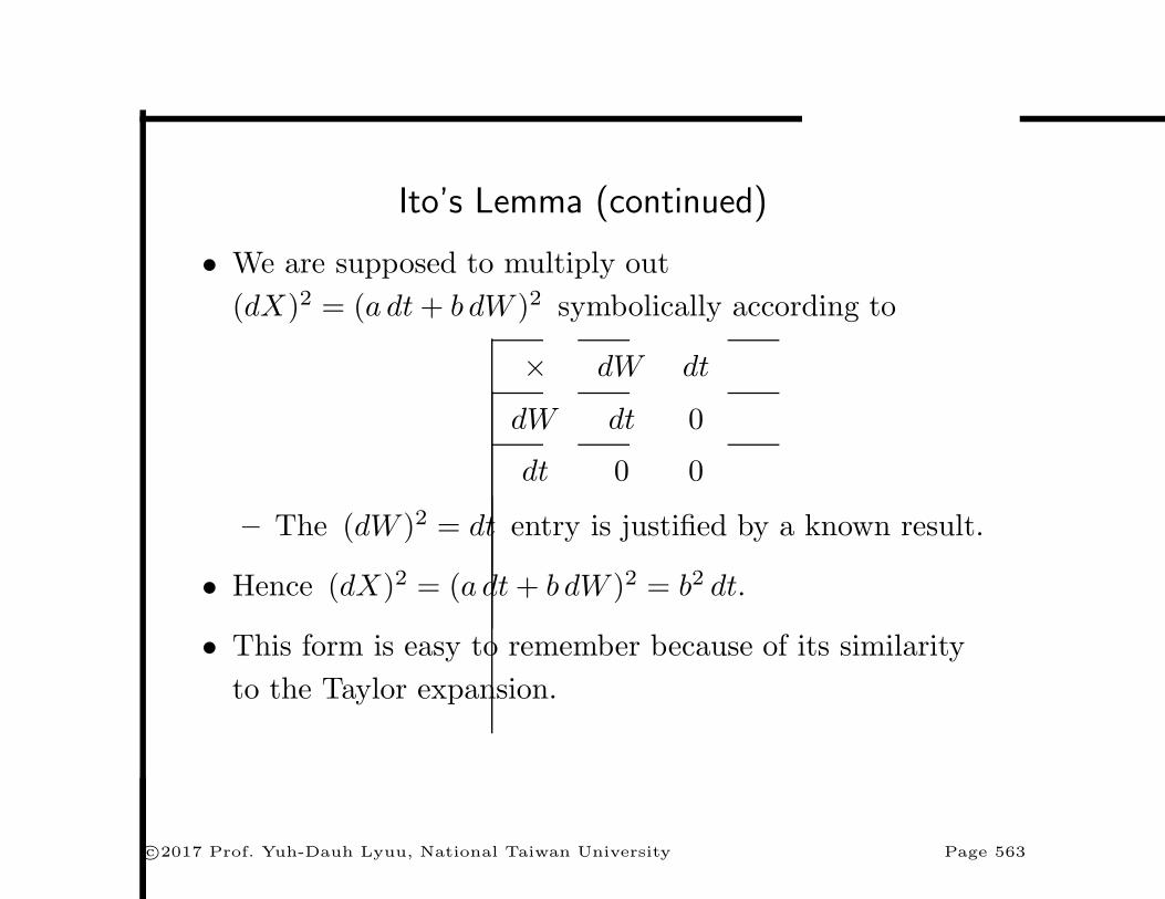
• We are supposed to multiply out

(dX)2 = (a dt+ b dW )2 symbolically according to

× dW dt

dW dt 0

dt 0 0

– The (dW )2 = dt entry is justified by a known result.

• Hence (dX)2 = (a dt+ b dW )2 = b2 dt.

• This form is easy to remember because of its similarity

to the Taylor expansion.



Theorem 21 (Higher-Dimensional Ito’s Lemma) Let

W1,W2, . . . ,Wn be independent Wiener processes and

XΔ= (X1, X2, . . . , Xm) be a vector process. Suppose

f : Rm → R is twice continuously differentiable and Xi is

an Ito process with dXi = ai dt+∑n

j=1 bij dWj. Then

df(X) is an Ito process with the differential,

df(X) =m∑i=1

fi(X) dXi +1

2

m∑i=1

m∑k=1

fik(X) dXi dXk,

where fiΔ= ∂f/∂Xi and fik

Δ= ∂2f/∂Xi∂Xk.



• The multiplication table for Theorem 21 is

× dWi dt

dWk δik dt 0

dt 0 0

in which

δik =

⎧⎨⎩ 1, if i = k,

0, otherwise.



• In applying the higher-dimensional Ito’s lemma, usually

one of the variables, say X1, is time t and dX1 = dt.

• In this case, b1j = 0 for all j and a1 = 1.

• As an example, let

dXt = at dt+ bt dWt.

• Consider the process f(Xt, t).



• Then

df =∂f

∂XtdXt +

∂f

∂tdt+

1

2

∂2f

∂X2t

(dXt)2

=∂f

∂Xt(at dt+ bt dWt) +

∂f

∂tdt

+1

2

∂2f

∂X2t

(at dt+ bt dWt)2

=

(∂f

∂Xtat +

∂f

∂t+

1

2

∂2f

∂X2t

b2t

)dt

+∂f

∂Xtbt dWt. (75)



Theorem 22 (Alternative Ito’s Lemma) Let

W1,W2, . . . ,Wm be Wiener processes and

XΔ= (X1, X2, . . . , Xm) be a vector process. Suppose

f : Rm → R is twice continuously differentiable and Xi is

an Ito process with dXi = ai dt+ bi dWi. Then df(X) is the

following Ito process,

df(X) =m∑i=1

fi(X) dXi +1

2

m∑i=1

m∑k=1

fik(X) dXi dXk.


Ito’s Lemma (concluded)

• The multiplication table for Theorem 22 is

× dWi dt

dWk ρik dt 0

dt 0 0

• Above, ρik denotes the correlation between dWi and

dWk.


Geometric Brownian Motion

• Consider geometric Brownian motion

Y (t)Δ= eX(t).

– X(t) is a (μ, σ) Brownian motion.

– By Eq. (69) on p. 531,

dX = μ dt+ σ dW.

• Note that

∂Y

∂X= Y,

∂2Y

∂X2= Y.


Geometric Brownian Motion (continued)

• Ito’s formula (74) on p. 562 implies

dY = Y dX + (1/2)Y (dX)2

= Y (μ dt+ σ dW ) + (1/2)Y (μ dt+ σ dW )2

= Y (μ dt+ σ dW ) + (1/2)Y σ2 dt.

• Hence

dY

Y=

(μ+ σ2/2

)dt+ σ dW. (76)

• The annualized instantaneous rate of return is μ+ σ2/2

(not μ).a

aConsistent with Lemma 11 (p. 283).


Geometric Brownian Motion (concluded)

• Similarly, suppose

dY

Y= μ dt+ σ dW.

• Then X(t)Δ= lnY (t) follows

dX =(μ− σ2/2

)dt+ σ dW.


Product of Geometric Brownian Motion Processes

• Let

dY

Y= a dt+ b dWY ,

dZ

Z= f dt+ g dWZ .

• Assume dWY and dWZ have correlation ρ.

• Consider the Ito process

UΔ= Y Z.


Product of Geometric Brownian Motion Processes(continued)

• Apply Ito’s lemma (Theorem 22 on p. 568):

dU = Z dY + Y dZ + dY dZ

= ZY (a dt+ b dWY ) + Y Z(f dt+ g dWZ)

+Y Z(a dt+ b dWY )(f dt+ g dWZ)

= U(a+ f + bgρ) dt+ Ub dWY + Ug dWZ .

• The product of correlated geometric Brownian motion

processes thus remains geometric Brownian motion.


Product of Geometric Brownian Motion Processes(continued)

• Note that

Y = exp[(a− b2/2

)dt+ b dWY

],

Z = exp[(f − g2/2

)dt+ g dWZ

],

U = exp[ (

a+ f − (b2 + g2

)/2)dt+ b dWY + g dWZ

].

– There is no bgρ term in U !


Product of Geometric Brownian Motion Processes(concluded)

• lnU is Brownian motion with a mean equal to the sum

of the means of lnY and lnZ.

• This holds even if Y and Z are correlated.

• Finally, lnY and lnZ have correlation ρ.


Quotients of Geometric Brownian Motion Processes

• Suppose Y and Z are drawn from p. 573.

• Let

UΔ= Y/Z.

• We now show thata

dU

U= (a− f + g2 − bgρ) dt+ b dWY − g dWZ .

(77)

• Keep in mind that dWY and dWZ have correlation ρ.

aExercise 14.3.6 of the textbook is erroneous.


Quotients of Geometric Brownian Motion Processes(concluded)

• The multidimensional Ito’s lemma (Theorem 22 on

p. 568) can be employed to show that

dU

= (1/Z) dY − (Y/Z2) dZ − (1/Z2) dY dZ + (Y/Z3) (dZ)2

= (1/Z)(aY dt+ bY dWY )− (Y/Z2)(fZ dt+ gZ dWZ)

−(1/Z2)(bgY Zρ dt) + (Y/Z3)(g2Z2 dt)

= U(a dt+ b dWY )− U(f dt+ g dWZ)

−U(bgρ dt) + U(g2 dt)

= U(a− f + g2 − bgρ) dt+ Ub dWY − Ug dWZ .


Forward Price

• Suppose S follows

dS

S= μ dt+ σ dW.

• Consider F (S, t)Δ= Sey(T−t) for some constants y and T .

• As F is a function of two variables, we need the various

partial derivatives of F (S, t) with respect to S and t.

• Note that in partial differentiation with respect to one

variable, other variables are held constant.a

aContributed by Mr. Sun, Ao (R05922147) on April 26, 2017.


Forward Prices (continued)

• Now,

∂F

∂S= ey(T−t),

∂2F

∂S2= 0,

∂F

∂t= −ySey(T−t).

• Then

dF = ey(T−t) dS − ySey(T−t) dt

= Sey(T−t) (μ dt+ σ dW )− ySey(T−t) dt

= F (μ− y) dt+ Fσ dW.


Forward Prices (concluded)

• One can also prove it by Eq. (75) on p. 567.

• Thus F follows

dF

F= (μ− y) dt+ σ dW.

• This result has applications in forward and futures

contracts.

• In Eq. (52) on p. 446, μ = r = y.

• SodF

F= σ dW,

a martingale.a

aIt is also consistent with p. 521.


Ornstein-Uhlenbeck (OU) Process

• The OU process:

dX = −κX dt+ σ dW,

where κ, σ ≥ 0.

• For t0 ≤ s ≤ t and X(t0) = x0, it is known that

E[X(t) ] = e−κ(t−t0) E[x0 ],

Var[X(t) ] =σ2

2κ

(1− e−2κ(t−t0)

)+ e−2κ(t−t0) Var[x0 ],

Cov[X(s),X(t) ] =σ2

2κe−κ(t−s)

[1− e−2κ(s−t0)

]

+e−κ(t+s−2t0) Var[x0 ].


Ornstein-Uhlenbeck Process (continued)

• X(t) is normally distributed if x0 is a constant or

normally distributed.

• X is said to be a normal process.

• E[x0 ] = x0 and Var[x0 ] = 0 if x0 is a constant.

• The OU process has the following mean reversion

property.

– When X > 0, X is pulled toward zero.

– When X < 0, it is pulled toward zero again.


Ornstein-Uhlenbeck Process (continued)

• A generalized version:

dX = κ(μ−X) dt+ σ dW,

where κ, σ ≥ 0.

• Given X(t0) = x0, a constant, it is known that

E[X(t) ] = μ+ (x0 − μ) e−κ(t−t0), (78)

Var[X(t) ] =σ2

2κ

[1− e−2κ(t−t0)

],

for t0 ≤ t.


Ornstein-Uhlenbeck Process (concluded)

• The mean and standard deviation are roughly μ and

σ/√2κ , respectively.

• For large t, the probability of X < 0 is extremely

unlikely in any finite time interval when μ > 0 is large

relative to σ/√2κ .

• The process is mean-reverting.

– X tends to move toward μ.

– Useful for modeling term structure, stock price

volatility, and stock price return.


Square-Root Process

• Suppose X is an OU process.

• Consider

VΔ= X2.

• Ito’s lemma says V has the differential,

dV = 2X dX + (dX)2

= 2√V (−κ

√V dt+ σ dW ) + σ2 dt

=(−2κV + σ2

)dt+ 2σ

√V dW,

a square-root process.


Square-Root Process (continued)

• In general, the square-root process has the stochastic

differential equation,

dX = κ(μ−X) dt+ σ√X dW,

where κ, σ ≥ 0 and X(0) is a nonnegative constant.

• Like the OU process, it possesses mean reversion: X

tends to move toward μ, but the volatility is

proportional to√X instead of a constant.


Square-Root Process (continued)

• When X hits zero and μ ≥ 0, the probability is one

that it will not move below zero.

– Zero is a reflecting boundary.

• Hence, the square-root process is a good candidate for

modeling interest rates.a

• The OU process, in contrast, allows negative interest

rates.b

• The two processes are related (see p. 586).

aCox, Ingersoll, & Ross (1985).bBut some rates have gone negative in Europe in 2015!


Square-Root Process (concluded)

• The random variable 2cX(t) follows the noncentral

chi-square distribution,a

χ

(4κμ

σ2, 2cX(0) e−κt

),

where cΔ= (2κ/σ2)(1− e−κt)−1.

• Given X(0) = x0, a constant,

E[X(t) ] = x0e−κt + μ

(1− e−κt

),

Var[X(t) ] = x0σ2

κ

(e−κt − e−2κt

)+ μ

σ2

2κ

(1− e−κt

)2,

for t ≥ 0.aWilliam Feller (1906–1970) in 1951.


Documents

Futures Price under the BOPM - 國立臺灣大學lyuu/finance1/2017/20170426.pdf · Martingale Pricing and Numerairea • Themartingalepricingformula(67)onp.518usesthe moneymarketaccountasnumeraire.b