Embed Size (px)
Citation preview
General Thermodynamicsfor
Process Simulation
Dr. Jungho Cho, ProfessorDepartment of Chemical Engineering
Dong Yang University

Thermodynamic Models built in Simulator
Four Criteria for Equilibria
Situation ConditionThermal Equilibrium
Mechanical Equilibrium
, Phase Equilibria (VLE, LLE)
Chemical Equilibrium
βα TT =βα PP =
li
vi μμ = 21 l
ili μμ =
0,
=
∂∂
PT
Gξ
Fugacity (or chemical potential) is defined as an escaping tendencyof a component ‘i’ in a certain phase into another phase.

Thermodynamic Models built in Simulator
Basic Phase Equilibria Relations
Vapor-liquid equilibrium calculations
The basic relationship for every component in vapor-liquidequilibrium is:
where: the fugacity of component i in the vapor phase
: the fugacity of component i in the liquid phase
( ) ( )il
iiv
i xPTfyPTf ,,ˆ,,ˆ =
vif̂l
if̂
(1)

Thermodynamic Models built in Simulator
Basic Phase Equilibria Relations
There are two methods for representing liquid fugacities.
- Equation of state method- Liquid activity coefficient method

Thermodynamic Models built in Simulator
Equation of State Method
The equation of state method defines fugacities as:
where:φiv is the vapor phase fugacity coefficientφil is the liquid phase fugacity coefficientyi is the mole fraction of i in the vapor xi is the mole fraction of i in the liquid P is the system pressure
Pyf ivi
vi φ̂ˆ = (2)
Pxf ili
li φ̂ˆ = (3)

Thermodynamic Models built in Simulator
Equation of State Method
We can then rewrite equation 1 as:
(4)
This is the standard equation used to represent vapor-liquid equilibrium using the equation-of-state method.
φiv and φil are both calculated by the equation-of-state.
Note that K-values are defined as:
ilii
vi xy φφ ˆˆ =
i
ii x
yK = (5)

Thermodynamic Models built in Simulator
Liquid Activity Coefficient Method (VLE)
The activity coefficient method defines liquid fugacities as:
The vapor fugacity is the same as the EOS approach:
Pyf ivi
vi φ̂ˆ =
where:iγ is the liquid activity coefficient of component i0
if is the standard liquid fugacity of component iviφ̂ is calculated from an equation-of-state model
We can then rewrite equation 1 as:0ˆ
iiiivi fxPy γφ =
0ˆiii
li fxf γ= (6)
(7)
(8)

Thermodynamic Models built in Simulator
Liquid Activity Coefficient Method (LLE)
• For Liquid-Liquid Equilibrium (LLE) the relationship is:
where the designators 1 and 2 represent the two separate liquid phases.
• Using the activity coefficient definition of fugacity, this can be rewritten and simplified as:
21 ˆˆ li
li ff =
2211 li
li
li
li xx γγ = (10)
(9)

Thermodynamic Models built in Simulator
K-values
The k-values can be calculated from:
Or
( )P
PPRTVP
xyK
vi
sati
lisat
isati
li
i
ii φ
φγ
ˆ
exp
−
==
vi
li
i
ii x
yKφφˆˆ
==
(11)
(12)

Thermodynamic Models built in Simulator
Example 2: Ideal Raoult’s Law
The preceding equation reduces to the following ideal Raoult’s law: vap
iii PxPy =
Example : Pxy plot at constant T(75oC). (P in kPa, T in oC)
22447.29452724.14ln 1 +
−=t
Pvap
20964.29722043.14ln 2 +
−=t
Pvap,
SolutionAt 75oC, kPaPvap 21.831 = and kPaP vap 98.411 =
The total pressure vapvap PxPxP 2211 += ( ) 1212 xPPPP vapvapvap −+=,
Vapor phase composition, ( ) PPx
xPPPPxy
vap
vapvapvap
vap11
1212
111 =
−+=
Thermodynamic Models built in Simulator
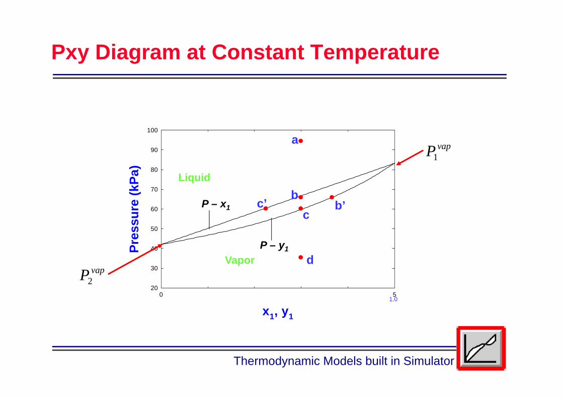
Pxy Diagram at Constant Temperature
x1, y1
0 5
Pres
sure
(kPa
)
20
30
40
50
60
70
80
90
100
1.0
vapP1
vapP2
a
bb’
cc’
d
Liquid
Vapor
P – x1
P – y1

Thermodynamic Models built in Simulator
Example 3: Slightly Non-ideal System
vapiiii PxPy γ=
For systems which the liquid phase behaves nonideally:
Relation between activity coefficient and excess Gibbs energy is as:( )
ijnPTi
ex
i nRTnG
≠
∂
∂=,,
/lnγ
As an example, excess Gibbs energy expression is as:
21xAxRTGex
=
Therefore, 1γ 2γand becomes.
( )221 exp Ax=γ ( )2
12 exp Ax=γ
So, ( )[ ] ( ) vapvap PxAxPxxAP 222111
21 exp1exp +−= ( )[ ]
PPxxAy
vap11
21
11exp −=

Thermodynamic Models built in Simulator
Prediction with Margules Equations
x1, y1
0.0 0.2 0.4 0.6 0.8 1.0
Pres
sure
(kPa
)
20
40
60
80
100
120
140
160
A = 0.0A = 0.5A = 1.0A = 2.0A = 3.0
Unstable

Thermodynamic Models built in Simulator
Deviations from Raoult’s Law (1 of 2) In general, you can expect non-ideality of unlike molecules. Either the size
and shape or the intermolecular interactions between components may be dissimilar. For short, these are called size and energy asymmetry. Energy asymmetry occurs between polar and non-polar molecules and also between different polar molecules.
In the majority of mixtures, activity coefficients is greater than unity. The result is a higher fugacity than ideal. The fugacity can be interpreted as the tendency to vaporize. If compounds vaporize mere than in an ideal solution, then they increase their average distance. So activity coefficients is greater than unity indicate repulsion between unlike molecules. If the repulsion is strong, liquid-liquid separation occurs. This is another mechanism that decreases close contact between unlike molecules.
If the activity coefficient is larger than unity, the system is said to show positive deviations from Raoult’s law. Negative deviations from Raoult’s law occur when the activity coefficient is smaller than unity.

Thermodynamic Models built in Simulator
Deviations from Raoult’s Law (2 of 2)
x1, y1
0.0 0.2 0.4 0.6 0.8 1.0
Pres
sure
(kPa
)
30
40
50
60
70
80
90
positive
negative
ideal
Sub-cooled Liquid
Super-heated Vapor

Thermodynamic Models built in Simulator
Isothermal Flash Calculations
Liquidfeed
T,P,Fzi
T & P
L, xi
Heater Valve
FlashDrum

Thermodynamic Models built in Simulator
Equilibrium Flash Vaporization
The equilibrium flash separator is the simplest equilibrium-stage process with which the designer must deal. Despite the fact that only one stage is involved, the calculation of the compositions and the relative amount of the vapor and liquid phases at any given pressure and temperature usually involves a tedious trial-and-error solution.
Buford D. Smith, 1963

Thermodynamic Models built in Simulator
Flash Calculation (1 of 4)
MESH Equation
Material Balance Equilbrium Relations Summation of Compositions Enthalpy(H) Balance

Thermodynamic Models built in Simulator
Flash Calculation (2 of 4)
Overall Material Balance
Component Material Balance
Equilibrium Relations
LVF +=
iii LxVyFz +=
iii xKy =
(1)
(2)
(3)

Thermodynamic Models built in Simulator
Flash Calculation (3 of 4)
Summation of Compositions
Defining
Combining (1) through (5), we obtain:
=i
ix 1
FV=φ
( ) ( )( ) =
−+−=
i i
ii
KKzF 0
111
φφ
(4b)
(5)
(6)
=i
iy 1(4a)
Thermodynamic Models built in Simulator
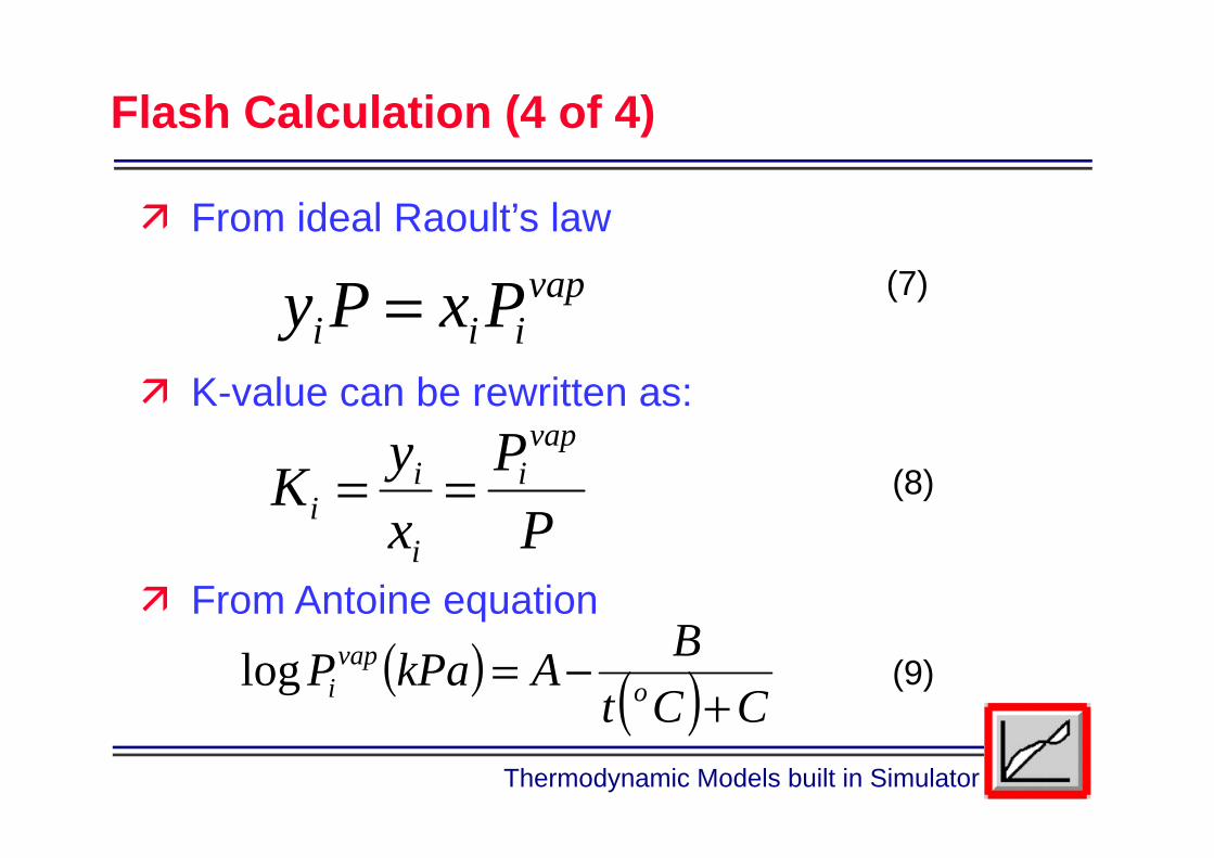
Flash Calculation (4 of 4)
From ideal Raoult’s law
K-value can be rewritten as:
From Antoine equation
vapiii PxPy =
PP
xyK
vapi
i
ii ==
( ) ( ) CCtBAkPaP o
vapi +
−=log
(7)
(8)
(9)

Thermodynamic Models built in Simulator
Antoine Coefficients
Benzene TolueneA 6.01788 6.08436B 1203.677 1347.620C 219.904 219.787
( ) ( ) CCtBAkPaP o
vapi +
−=log

Thermodynamic Models built in Simulator
Rachford-Rice Function
φ0.0 0.2 0.4 0.6 0.8 1.0
F(φ)
-0.15
-0.10
-0.05
0.00
0.05
0.10
707.0=φ
( ) ( )( ) =
−+−=
i i
ii
KKzF 0
111
φφ

Thermodynamic Models built in Simulator
Flash Calculation Results (1 of 3)
Vapor Flowrate (K-mole/hr)
Liquid Flowrate (K-mole/hr)
(1)
(2)
( ) 7.70)707.0(100 =×== φFV
3.297.70100 =−=−= VFL

Thermodynamic Models built in Simulator
Flash Calculation Results (2 of 3)
Mole Fraction at the liquid phase
Mole Fraction at the vapor phase
(3)
(4)
( )11 −+=
i
ii K
zxφ
4479.0=Bx 5521.0=Tx
(5)
(6)
( )11 −+==
i
iiiii K
zKxKyφ
6631.0=By 3369.0=Ty

Thermodynamic Models built in Simulator
Flash Calculation Results (3 of 3)
Mole Fraction of Benzene0.0 0.1 0.2 0.3 0.4 0.5 0.6 0.7 0.8 0.9 1.0
Pre
ssur
e (k
Pa)
60
80
100
120
140
160
180
200
4329.0=Bx6429.0=By
Thermodynamic Models built in Simulator
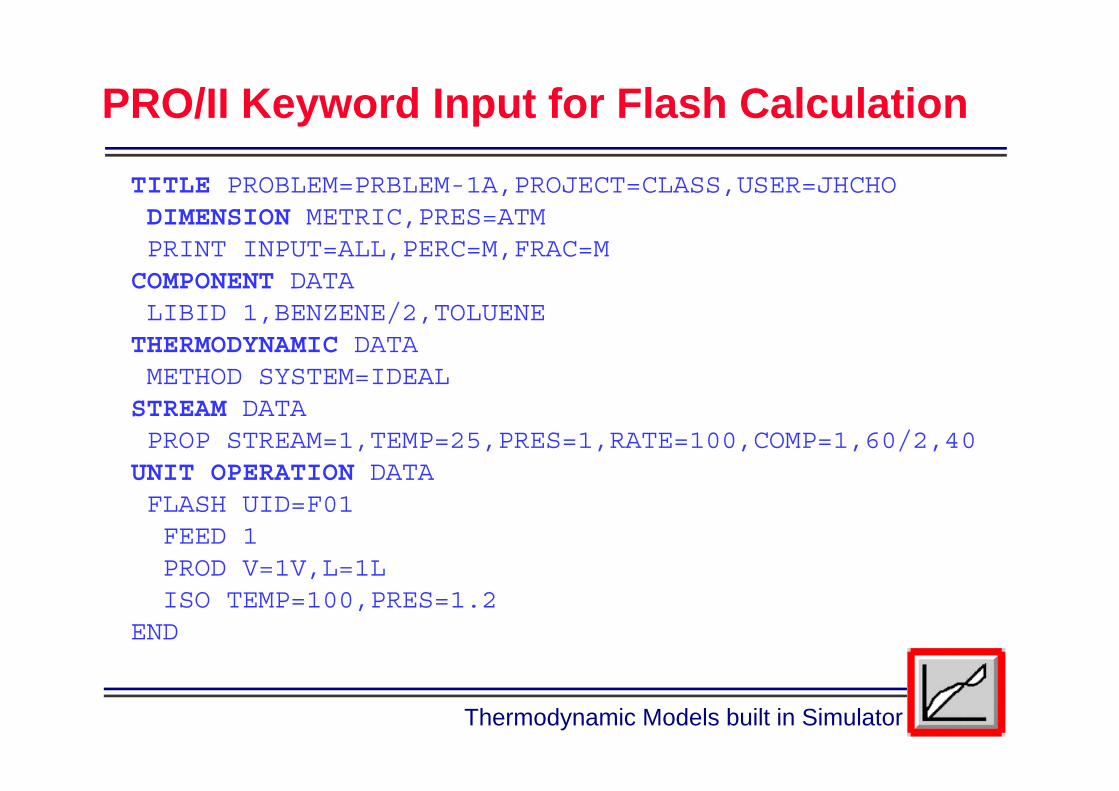
PRO/II Keyword Input for Flash Calculation
TITLE PROBLEM=PRBLEM-1A,PROJECT=CLASS,USER=JHCHODIMENSION METRIC,PRES=ATMPRINT INPUT=ALL,PERC=M,FRAC=M
COMPONENT DATALIBID 1,BENZENE/2,TOLUENE
THERMODYNAMIC DATAMETHOD SYSTEM=IDEAL
STREAM DATAPROP STREAM=1,TEMP=25,PRES=1,RATE=100,COMP=1,60/2,40
UNIT OPERATION DATAFLASH UID=F01FEED 1PROD V=1V,L=1LISO TEMP=100,PRES=1.2
END

Thermodynamic Models built in Simulator
PRO/II Output Summary for Flash Calculation
STREAM ID 1 1L 1VNAMEPHASE LIQUID LIQUID VAPOR
FLUID MOLAR FRACTIONS1 BENZENE 0.6000 0.4476 0.66292 TOLUENE 0.4000 0.5524 0.3371
TOTAL RATE, KG-MOL/HR 100.0000 75.6710 24.3290
TEMPERATURE, C 25.0000 100.0000 100.0000PRESSURE, ATM 1.0000 1.2000 1.2000ENTHALPY, M*KCAL/HR 0.0865 0.2800 0.2681MOLECULAR WEIGHT 85.1285 85.8632 82.8433MOLE FRAC VAPOR 0.0000 0.0000 1.0000MOLE FRAC LIQUID 1.0000 1.0000 0.0000

Thermodynamic Models built in Simulator
PRO/II BVLE Analysis

Thermodynamic Models built in Simulator
Dew & Bubble Point Calculation
Dew Point is the very state at which condensation is about to occur. Dew Point Temperature Calculation at a Given Pressure Dew Point Pressure Calculation at a Given Temperature Vapor Fraction is ‘1’ at Dew Point
Bubble Point is the very state at which vaporization is about to occur. Bubble Point Temperature Calculation at a Given Pressure Bubble Point Pressure Calculation at a Given Temperature Vapor Fraction is ‘0’ at Bubble Point

Thermodynamic Models built in Simulator
Ex-1: Bubble Point Failure Case
Calculate the bubble point pressure at 85oC of the following stream. Did you get a converged solution? If not, why?
Use SRK for your simulation.
Component Mole %C1 65C2 15C3 15IC4 5
Save as Filename:
EX-1.inp

Thermodynamic Models built in Simulator
Difference between Gas and Vapor
For gas, T > Tc
For vapor, T < Tc
T: System temperature, Tc: Critical temperature
“Methane Gas” but not “Methane Vapor” “Water Vapor” but not “Water Gas”

Thermodynamic Models built in Simulator
Ex-2: C7 Plus Heavy Cut Characterization
Calculate the bubble pressure at 45oC and dew temperature at 1.5bar of the following stream. Regard C6+ as NC6(1), NC7(2) and NC8(3) and compare the results. Use SRK for your simulation.
Component Mole %C1 5
C2 10
C3 15
IC4 10
NC4 20
IC5 15
NC5 20
C6+ 5
Save as Filename: EX-2A.inp for NC6, EX-2B.inp for NC7, EX-2C.inp for NC8

Thermodynamic Models built in Simulator
Results for EX-2
Characterization of heavycut is very important in the calculation of dew point temperature.
EX-2A.inp, EX-2B.inp, EX-2C.inp
Bubble Pat 45oC
Dew Tat 1.5bar
C6 Plus
18.505 30.519 NC618.561 42.783 NC718.669 59.585 NC8

Thermodynamic Models built in Simulator
Results for EX-2A (C6+ NC6)

Thermodynamic Models built in Simulator
Results for EX-2B (C6+ NC7)

Thermodynamic Models built in Simulator
Results for EX-2C (C6+ NC8)

Thermodynamic Models built in Simulator
The End of General Thermodynamics
The End….