Title

Global Classical and Weak Solutions to the Three-DimensionalFull Compressible Navier-Stokes System with Vacuum andLarge Oscillations (Mathematical Analysis in Fluid and GasDynamics)

Author(s) HUANG, Xiangdi; LI, Jing

Citation 数理解析研究所講究録 (2013), 1830: 98-118

Issue Date 2013-04

URL http://hdl.handle.net/2433/194822

Right

Type Departmental Bulletin Paper

Textversion publisher

Kyoto University

Global Classical and Weak Solutions to theThree-Dimensional Full Compressible Navier-Stokes

System with Vacuum and Large Oscillations*

Xiangdi HUANGa, Jing LIba NCMIS, Academy of Mathematics and System Sciences,Chinese Academy of Sciences, Beijing 100190,P. R. China

b Institute of Applied Mathematics, AMSS,& Hua Loo-Keng Key Laboratory of Mathematics,

Chinese Academy of Sciences, Beijing 100190, P. R. China

The motion of compressible viscous, heat-conductive polytropic fluid reads

$[Matrix]$ (0.1)

where $\mathfrak{D}(u)$ is the deformation tensor:

$\mathfrak{D}(u)=\frac{1}{2}(\nabla u+(\nabla u)^{tr})$ .

Here $\rho,$$u=(u^{1}, u^{2}, u^{3})^{tr},$ $e,$ $P(\rho, e)$ , and $\theta$ represent respectively the fluid density, veloc-

ity, specific intemal energy, pressure, and absolute temperature. The constant viscosity$co$efficients $\mu$ and $\lambda$ satisfy the physical restrictions:

$\mu>0,$ $2\mu+3\lambda\geq 0$ . (0.2)

We study the ideal polytropic fluids so that $P$ and $e$ are given by the state equations:

$P( \rho, e)=(\gamma-1)\rho e=R\rho\theta, e=\frac{R\theta}{\gamma-1}$ , (0.3)

where $\gamma>1$ is the adiabatic constant, and $R,$ $\kappa$ are both positive constants.

Let $\tilde{\rho},\tilde{\theta}$ both be fixed positive constants. We look for the solutions $(\rho(x, t), u(x, t), \theta(x, t))$ ,with the far field behavior:

$(\rho, u, \theta)(x, t)arrow(\tilde{\rho}, 0,\tilde{\theta})$ , as $|x|arrow\infty,$ $t>0$ , (0.4)

$(\rho, \rho u, \rho\theta)(x, t=0)=(\rho 0, \rho 0u0, \rho 0\theta 0)(x) , x\in\mathbb{R}^{3}$ , (0.5)

Moreover, for classical solutions, we replace the initial condition with

$(\rho, u, \theta)(x, t=0)=(\rho_{0}, u0, \theta_{0})$ , $x\in \mathbb{R}^{3}$ , with $\rho 0\geq 0,$ $\theta_{0}\geq 0$ . (0.6)

’This research is partially supported by SRF for ROCS, SEM, and National Science Foundation ofChina under grant 10971215. Email: xdhuang@amss.ac.cn (X. Huang), ajingli@gmail.com (J. Li).

数理解析研究所講究録第 1830巻 2013年 98-118 98

We assume that $\tilde{\rho}=\tilde{\theta}=1$ . and define the initial energy $C_{0}$ as follows:

$C_{0}= \Delta\frac{1}{2}\int\rho_{0}|u_{0}|^{2}dx+R\int(\rho_{0}\log\rho_{0}-\rho_{0}+1)dx$

(0.7)$+ \frac{R}{\gamma-1}\int\rho_{0}(\theta_{0}-\log\theta_{0}-1)dx+\frac{R}{2(\gamma-1)}\int\rho_{0}(\theta_{0}-1)^{2}dx.$

Then the first main result in this paper can be stated as follows:

Theorem 0.1 For given numbers $M>0$ (not necessarily small), $q\in(3,6)$ , and $\overline{\rho}>2,$

suppose that the initial data $(\rho_{0}, u_{0}, \theta_{0})$ satisfies$\rho_{0}-1\in H^{2}\cap W^{2,q}, u_{0}\in H^{2}, \theta_{0}-1\in H^{2}$, (0.8)

$0 \leq\inf\rho_{0}\leq\sup\rho 0<\overline{\rho}, \inf\theta_{0}\geq 0, \Vert\nabla u_{0}\Vert_{L^{2}}\leq M$ , (0.9)

and the compatibility conditions:

$-\mu\triangle u_{0}-(\mu+\lambda)\nabla divu_{0}+R\nabla(\rho_{0}\theta_{0})=\sqrt{\rho_{0}}g_{1}$ , (0.10)

$\kappa\triangle\theta_{0}+\frac{\mu}{2}|\nabla u_{0}+(\nabla uo)^{tr}|^{2}+\lambda(divu_{0})^{2}=\sqrt{\rho_{0}}g_{2},$ (0.11)

with $g_{1},$ $g_{2}\in L^{2}$ . Then there exists a positive constant $\epsilon$ depending only on $\mu,$$\lambda,$

$\kappa,$ $R,$

$\gamma,\overline{\rho}$ , and $M$ such that if$C_{0}\leq\epsilon$ , (0.12)

the Cauchy problem (0.1) $(o.4)(0.6)$ has a unique global classical solution $(\rho, u, \theta)$ in$\mathbb{R}^{3}\cross(0, \infty)$ satisfying

$0\leq\rho(x, t)\leq 2\overline{\rho}, \theta(x, t)\geq 0, x\in \mathbb{R}^{3}, t\geq 0$, (0.13)

$\{\begin{array}{l}\rho-1\in C([0, T];H^{2}\cap W^{2,q}) , (u, \theta-1)\in C([0, T];H^{2}) ,u\in L^{\infty}(\tau, T;H^{3}\cap W^{3,q}) , \theta-1\in L^{\infty}(\tau, T;H^{4}) ,(u_{t}, \theta_{t})\in L^{\infty}(\tau, T;H^{2})\cap H^{1}(\tau, T;H^{1}) ,\end{array}$ (0.14)

and the following large-time behavior:

$\lim_{tarrow\infty}(\Vert\rho(\cdot, t)-1\Vert_{L^{p}}+\Vert\nabla u(\cdot, t)\Vert_{L^{r}}+\Vert\nabla\theta(\cdot, t)\Vert_{L^{r}})=0$ , (0.15)

with any$0<\tau<T<\infty, p\in(2, \infty) , r\in[2,6)$ . (0.16)

The next result of this paper will treat the weak solutions. To begin with, we givethe definition of weak solutions.

Definition 0.1 We say that $( \rho, u, E=\frac{1}{2}|u|^{2}+\frac{R}{\gamma-1}\theta)$ is a weak solution to Cauchyproblem $(0.1)(o.4)(0.5)$ provided that

$\rho-1\in L_{1oc}^{\infty}([0, \infty);L^{2}\cap L^{\infty}(\mathbb{R}^{3})) , u, \theta-1\in L^{2}(0, \infty;H^{1}(\mathbb{R}^{3}))$ ,

and that for all test functions $\psi\in \mathcal{D}(\mathbb{R}^{3}\cross(-\infty, \infty))$ ,

$\int_{\mathbb{R}^{3}}\rho 0\psi(\cdot, 0)dx+\int_{0}^{\infty}\int_{\mathbb{R}^{3}}(\rho\psi_{t}+\rho u\cdot\nabla\psi)dxdt=0$, (0.17)

99

$\int_{\mathbb{R}^{3}}\rho_{0}u_{0}^{j}\psi(\cdot, 0)dx+\int_{0}^{\infty}\int_{\mathbb{R}^{3}}(\rho u^{j}\psi_{t}+\rho u^{j}u\cdot\nabla\psi+P(\rho, \theta)\psi_{x_{j}})dxdt$

(0.18)$- \int_{0}^{\infty}\int_{\mathbb{R}^{3}}(\mu\nabla u^{j}\cdot\nabla\psi+(\mu+\lambda)(divu)\psi_{x_{j}})dxdt=0, j=1,2,3,$

$\int_{\mathbb{R}^{3}}(\frac{1}{2}\rho 0|u_{0}|^{2}+\frac{R}{\gamma-1}\rho_{0}\theta_{0})\psi(\cdot, 0)dx$

$= \int_{0}^{\infty}\int_{\mathbb{R}^{3}}(\rho E\psi_{t}+(\rho E+P)u\cdot\nabla\psi)dxdt$ (0.19)

$- \int_{0}^{\infty}\int_{\mathbb{R}^{3}}(\kappa\nabla\theta+\frac{1}{2}\mu\nabla(|u|^{2})+\mu u\cdot\nabla u+\lambda udivu)\cdot\nabla\psi dxdt.$

We also define

$;=\Delta f_{t}+u\cdot\nabla f, G=\Delta(2\mu+\lambda)divu-R(\rho\theta-1) , \omega=\Delta\nabla\cross u$, (0.20)

which are the material derivative of $f$ , the effective viscous flux, and the vorticityrespectively. We now state our second main result as follows:

Theorem 0.2 For given numbers $M>0$ (not necessarily small), and $\overline{\rho}>2$ , thereexists a positive constant $\epsilon$ depending only on $\mu,$

$\lambda,$$\kappa,$ $R,$ $\gamma,\overline{\rho}$ , and $M$ such that if the

initial data $(\rho_{0}, u_{0}, \theta_{0})$ satisfies (0.9) and

$C_{0}\leq\epsilon$ , (0.21)

with $C_{0}$ as in (0.7), there is a global weak solution $(\rho, u, \theta)$ to the Cauchy problem (0.1)(0.4) $(0.5)$ satisfying

$\rho-1\in C([0, \infty);L^{2}\cap L^{p}) , (\rho u, \rho|u|^{2}, \rho(\theta-1))\in C([0, \infty);H^{-1})$, (0.22)

$u\in C((O, \infty);L^{2}) , \theta-1\in C((0, \infty);W^{1,r})$, (0.23)

$u(\cdot, t), \omega(\cdot, t), G(\cdot, t), \nabla\theta(\cdot, t)\in H^{1}, t>0$, (0.24)

$\rho\in[0,2\overline{\rho}]$ a.e., $\theta\geq 0$ a.e., (0.25)

and the following large-time behavior:

$\lim_{tarrow\infty}(\Vert\rho(\cdot, t)-1\Vert_{Lp}+\Vert u(\cdot, t)\Vert_{L^{p}\cap L}\infty+\Vert\nabla\theta(\cdot, t)\Vert_{L^{r}})=0$, (0.26)

with any $p,$ $r$ as in (0.16). In addition, there exists some positive constant $C$ dependingonly on $\mu,$

$\lambda,$$\kappa,$ $R,$ $\gamma,\overline{\rho}$, and $M$, such that, for $\sigma(t)=\Delta\min\{1, t\}$ , the following estimates

hold$\sup \Vert u\Vert_{H^{1}}+\int_{0}^{\infty}\int|(\rho u)_{t}+div(\rho u\otimesu)|^{2}dxdt\leq C$ , (0.27)

$t\in(0,\infty)$

$\sup_{t\in(0,\infty)}\int((\rho-1)^{2}+\rho|u|^{2}+\rho(\theta-1)^{2})dx$

(0.28)$+ \int_{0}^{\infty}(\Vert Vu\Vert_{L^{2}}^{2}+\Vert\nabla\theta\Vert_{L^{2}}^{2})dt\leq CC_{0}^{1/4},$

$\sup_{t\in(0,\infty)}(\sigma^{2}\Vert\nabla u\Vert_{L^{6}}^{2}+\sigma^{4}\Vert\theta-1\Vert_{H^{2}}^{2})$

(0.29)$+ \int_{0}^{\infty}(\sigma^{2}\Vert u_{t}\Vert_{L^{2}}^{2}+\sigma^{2}\Vert\nabla\dot{u}\Vert_{L^{2}}^{2}+\sigma^{4}\Vert\theta_{t}\Vert_{H^{1}}^{2})dt\leq CC_{0}^{1/8}$

100

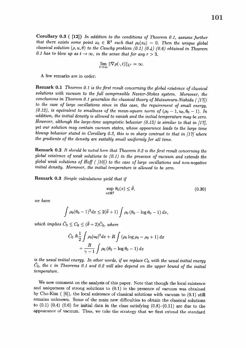
Corollary 0.3 ([12]) In addition to the conditions of Theorem 0.1, assume furtherthat there exists some point $x_{0}\in \mathbb{R}^{3}$ such that $\rho_{0}(x_{0})=0$ . Then the unique globalclassical solution $(\rho, u, \theta)$ to the Cauchy problem (0.1) (0.4) (0.6) obtained in Theorem0.1 has to blow up as $tarrow\infty$ , in the sense that for any $r>3,$

$\lim_{tarrow\infty}\Vert\nabla\rho(\cdot, t)\Vert_{L^{r=\infty}}.$

A few remarks are in order:

Remark 0.1 Theorem 0.1 is the first result concerning the global existence of classicalsolutions with vacuum to the full compressible Navier-Stokes system. Moreover, theconclusions in Theorem 0.1 genemlize the classical theory of Matsumura-Nishida $([17J)$to the case of large oscillations since in this case, the requirement of small energy,(0.12), is equivalent to smallness of the mean-square norm of $(\rho_{0}-1, u_{0}, \theta_{0}-1)$ . Inaddition, the initial density is allowed to vanish and the initial temperature may be zero.However, although the large-time asymptotic behavior (0.15) $i_{s}s$ similar to that in $[17J,$

yet our solution may contain vacuum states, whose appearance leads to the large timeblowup behavior stated in Corollary 0.3, this is in sharp contrast to that in $[17J$ wherethe gmdients of the density are suitably small uniformly for all time.

Remark 0.2 It should be noted here that Theorem 0.2 is the first result concerning theglobal existence of weak solutions to (0.1) in the presence of vacuum and extends theglobal weak solutions of Hoff ([$1OJ$) to the case of large oscillations and non-negativeinitial density. Moreover, the initial temperature is allowed to be zero.

Remark 0.3 Simple calculations yield that if

$\sup_{x\in \mathbb{R}^{3}}\theta_{0}(x)\leq\overline{\theta}$, (0.30)

we have

$\int\rho_{0}(\theta_{0}-1)^{2}dx\leq 2(\overline{\theta}+1)\int\rho_{0}(\theta_{0}-\log\theta_{0}-1)dx,$

which implies $\tilde{C}_{0}\leq C_{0}\leq(\overline{\theta}+2)\tilde{C}_{0}$ , where

$\tilde{c}_{0=\frac{1}{2}}^{\triangle}\int\rho_{0}|u_{0}|^{2}dx+R\int(\rho_{0}\log\rho_{0}-\rho_{0}+1)dx$

$+ \frac{R}{\gamma-1}\int\rho 0(\theta_{0}-\log\theta_{0}-1)dx$

$is\sim the$ usual initial energy. In other words, if we replace $C_{0}$ with the usual initial energy$C_{0}$ , the $\epsilon$ in Theorems 0.1 and 0.2 will also depend on the upper bound of the initialtemperature.

We now comment on the analysis of this paper. Note that though the local existenceand uniqueness of strong solutions to (0.1) in the presence of vacuum was obtainedby Cho-Kim ([6]), the local existence of classical solutions with vacuum to (0.1) stillremains unknown. Some of the main new difficulties to obtain the classical solutionsto (0.1) (0.4) (0.6) for initial data in the class satisfying $(0.8)-(0.11)$ are due to theappearance of vacuum. Thus, we take the strategy that we first extend the standard

101

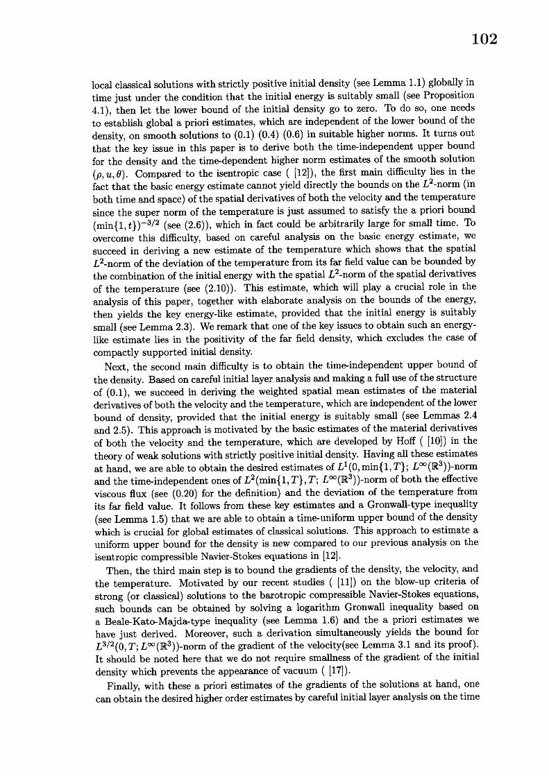
$10$cal classical solutions with strictly positive initial density (see Lemma 1.1) globally intime just under the condition that the initial energy is suitably small (see Proposition4.1), then let the lower bound of the initial density go to zero. To do so, one needsto estabhsh global a priori estimates, which are independent of the lower bound of thedensity, on smooth solutions to (0.1) (0.4) (0.6) in suitable higher norms. It turns outthat the key issue in this paper is to derive both the time-independent upper boundfor the density and the time-dependent higher norm estimates of the smooth solution$(\rho, u, \theta)$ . Compared to the isentropic case ([12]), the first main difficulty lies in thefact that the basic energy estimate cannot yield directly the bounds on the $L^{2}$-norm (in

both time and space) of the spatial derivatives of both the velocity and the temperaturesince the super norm of the temperature is just assumed to satisfy the a priori bound$( \min\{1, t\})^{-3/2}$ (see (2.6)), which in fact could be arbitrarily large for small time. Toovercome this difficulty, based on careful analysis on the basic energy estimate, wesucceed in deriving a new estimate of the temperature which shows that the spatial$L^{2}$-norm of the deviation of the temperature from its far field value can be bounded bythe combination of the initial energy with the spatial $L^{2}$-norm of the spatial derivativesof the temperature (see (2.10)). This estimate, which will play a crucial role in theanalysis of this paper, together with elaborate analysis on the bounds of the energy,then yields the key energy-like estimate, provided that the initial energy is suitablysmall (see Lemma 2.3). We remark that one of the key issues to obtain such an energy-like estimate hes in the positivity of the far field density, which excludes the case ofcompactly supported initial density.

Next, the second main difficulty is to obtain the timeindependent upper bound ofthe density. Based on careful initial layer analysis and making a full use of the structureof (0.1), we succeed in deriving the weighted spatial mean estimates of the materialderivatives of both the velocity and the temperature, which are independent of the lowerbound of density, provided that the initial energy is suitably small (see Lemmas 2.4and 2.5). This approach is motivated by the basic estimates of the material derivativesof both the velocity and the temperature, which are developed by Hoff ([10]) in thetheory of weak solutions with strictly positive initial density. Having all these estimatesat hand, we are able to obtain the desired estimates of $L^{1}(0, \min\{1, T\};L^{\infty}(\mathbb{R}^{3}))$-normand the time-independent ones of $L^{2}( \min\{1, T\}, T;L^{\infty}(\mathbb{R}^{3}))$-norm of both the effectiveviscous flux (see (0.20) for the definition) and the deviation of the temperature fromits far field value. It follows from these key estimates and a Gronwall-type inequality(see Lemma 1.5) that we are able to obtain a time-uniform upper bound of the densitywhich is crucial for global estimates of classical solutions. This approach to estimate auniform upper bound for the density is new compared to our previous analysis on theisentropic compressible Navier-Stokes equations in [12].

Then, the third main step is to bound the gradients of the density, the velocity, andthe temperature. Motivated by our recent studies ([11]) on the blow-up criteria ofstrong (or classical) solutions to the barotropic compressible Navier-Stokes equations,such bounds can be obtained by solving a logarithm Gronwall inequality based ona Beale-Kato-Majda-type inequality (see Lemma 1.6) and the a priori estimates wehave just derived. Moreover, such a derivation simultaneously yields the bound for$L^{3/2}(0, T;L^{\infty}(\mathbb{R}^{3}))$-norm of the gradient of the velocity(see Lemma 3.1 and its proof).

It should be noted here that we do not require smallness of the gradient of the initialdensity which prevents the appearance of vacuum ([17]).

Finally, with these a priori estimates of the gradients of the solutions at hand, onecan obtain the desired higher order estimates by careful initial layer analysis on the time

102

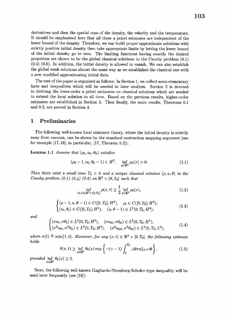
derivatives and then the spatial ones of the density, the velocity and the temperature.It should be emphasized here that all these a priori estimates are independent of thelower bound of the density. Therefore, we can build proper approximate solutions withstrictly positive initial density then take appropriate limits by letting the lower boundof the initial density go to zero. The limiting functions having exactly the desiredproperties are shown to be the global classical solutions to the Cauchy problem (0.1)(0.4) (0.6). In addition, the initial density is allowed to vanish. We can also establishthe global weak solutions almost the same way as we established the classical one witha new modified approximating initial data.

The rest of the paper is organized as follows: In Section 1, we collect some elementaryfacts and inequalities which will be needed in later analysis. Section 2 is devotedto deriving the lower-order a priori estimates on classical solutions which are neededto extend the local solution to all time. Based on the previous results, higher-orderestimates are established in Section 3. Then finally, the main results, Theorems 0.1and 0.2, are proved in Section 4.

1 Preliminaries

The following well-known local existence theory, where the initial density is strictlyaway from vacuum, can be shown by the standard contraction mapping argument (seefor example [17, 18], in particular, [17, Theorem 5.2] $)$ .

Lemma 1. 1 $A$ ssume that $(\rho_{0}, u_{0}, \theta_{0})$ satisfies

$( \rho_{0}-1, u_{0}, \theta_{0}-1)\in H^{3}, \inf_{x\in \mathbb{R}^{3}}\rho_{0}(x)>0$. (1.1)

Then there exist a small time $T_{0}>0$ and a unique classical solution $(\rho, u, \theta)$ to theCauchy pmblem (0.1) (0.4) (0.6) on $\mathbb{R}^{3}\cross(0, T_{0}]$ such that

$\inf_{(x,t)\in \mathbb{R}^{3}\cross(0,T_{0}]}\rho(x, t)\geq\frac{1}{2}\inf_{x\in \mathbb{R}^{3}}\rho_{0}(x)$, (1.2)

$\{\begin{array}{l}(\rho-1, u, \theta-1)\in C([O, T_{0}];H^{3}) , \rho_{t}\in C([0, T_{0}];H^{2}) ,(u_{t}, \theta_{t})\in C([0, T_{0}];H^{1}) , (u, \theta-1)\in L^{2}(0, T_{0};H^{4}) ,\end{array}$ (1.3)

and

$\{\begin{array}{l}(\sigma u_{t}, \sigma\theta_{t})\in L^{2}(0, T_{0};H^{3}) , (\sigma u_{tt}, \sigma\theta_{tt})\in L^{2}(0, T_{0};H^{1}) ,(\sigma^{2}u_{tt}, \sigma^{2}\theta_{tt})\in L^{2}(0, T_{0};H^{2}) , (\sigma^{2}u_{ttt}, \sigma^{2}\theta_{ttt})\in L^{2}(0, T_{0};L^{2}) ,\end{array}$ (1.4)

where $\sigma(t)=\Delta\min\{1, t\}$ . Moreover, for any $(x, t)\in \mathbb{R}^{3}\cross[0, T_{0}]$ , the following estimateholds

$\theta(x, t)\geq\inf_{x\in \mathbb{R}^{3}}\theta_{0}(x)\exp\{-(\gamma-1)\int_{0}^{T_{0}}\Vert divu\Vert_{L}\infty dt\}$ , (1.5)

provided $\inf_{x\in \mathbb{R}^{3}}\theta_{0}(x)\geq 0.$

Next, the following well-known Gagliardo-Nirenberg-Sobolev-type inequality will beused later frequently (see [19]).

103

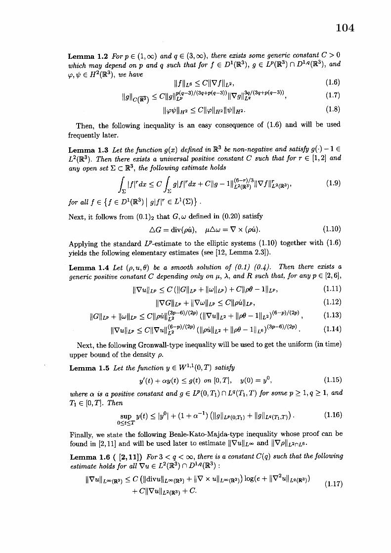
Lemma 1.2 For $p\in(1, \infty)$ and $q\in(3, \infty)$ , there exists some generic constant $C>0$

which may depend on $p$ and $q$ such that for $f\in D^{1}(\mathbb{R}^{3}),$ $g\in L^{p}(\mathbb{R}^{3})\cap D^{1,q}(\mathbb{R}^{3})$ , and$\varphi,$

$\psi\in H^{2}(\mathbb{R}^{3})$ , we have$\Vert f\Vert_{L^{6}}\leq C\Vert\nabla f\Vert_{L^{2}}$ , (1.6)

$\Vert g\Vert_{c(\overline{\mathbb{R}^{3}})}\leq C\Vert g\Vert_{L^{p}}^{p(q-3)/(3q+p(q-3))}\Vert\nabla g\Vert_{L^{q}}^{3q/(3q+p(q-3))}$, (1.7)

$\Vert\varphi\psi\Vert_{H^{2}}\leq C\Vert\varphi\Vert_{H^{2}}\Vert\psi\Vert_{H^{2}}$ . (1.8)

Then, the following inequality is an easy consequence of (1.6) and will be usedfrequently later.

Lemma 1.3 Let the function $g(x)$ defined in $\mathbb{R}^{3}$ be non-negative and satisfy $g(\cdot)-1\in$

$L^{2}(\mathbb{R}^{3})$ . Then there exists a universal positive constant $C$ such that for $r\in[1,2]$ andany open set $\Sigma\subset \mathbb{R}^{3}$ , the following estimate holds

$\int_{\Sigma}|f|^{r}dx\leq C\int_{\Sigma}g|f|^{r}dx+C\Vert g-1\Vert_{L^{2}(\mathbb{R}^{3})}^{(6-r)/3}\Vert\nabla f\Vert_{L^{2}(\mathbb{R}^{3})}^{r}$ , (1.9)

for all $f\in\{f\in D^{1}(\mathbb{R}^{3})|g|f|^{r}\in L^{1}(\Sigma)\}.$

Next, it follows from $(0.1)_{2}$ that $G,$ $\omega$ defined in (0.20) satisfy

$\triangle G=div(\rho\dot{u}) , \mu\triangle\omega=\nabla\cross(\rho\dot{u})$ . (1.10)

Applying the standard $L^{p}$-estimate to the elhptic systems (1.10) together with (1.6)yields the following elementary estimates (see [12, Lemma 2.3]).

Lemma 1.4 Let $(\rho, u, \theta)$ be a smooth solution of (0.1) $(o.4)$ . Then there exists ageneric positive constant $C$ depending only on $\mu,$

$\lambda$ , and $R$ such that, for any $p\in[2,6],$

$\Vert\nabla u\Vert_{Lp}\leq C(\Vert G\Vert_{L^{p}}+\Vert\omega\Vert_{Lp})+C\Vert\rho\theta-1\Vert_{L^{p}}$, (1.11)

$\Vert\nabla G\Vert_{Lp}+\Vert\nabla\omega\Vert_{L^{p}}\leq C\Vert\rho\dot{u}\Vert_{Lp}$ , (1.12)

$\Vert G\Vert_{Lp}+\Vert\omega\Vert_{Lp}\leq C\Vert\mu\dot{r}\Vert_{L^{2}}^{(3p-6)/(2p)} (\Vert Vu\Vert_{L^{2}}+\Vert\rho\theta-1\Vert_{L^{2}})^{(6-p)/(2p)}$ , (1.13)

$\Vert$ Vu $\Vert_{L^{p}}\leq C\Vert\nabla u\Vert_{L^{2}}^{(6-p)/(2p)}(\Vert\dot{\mu}\iota\Vert_{L^{2}}+\Vert\rho\theta-1\Vert_{L^{6}})^{(3p-6)/(2p)}$ . (1.14)

Next, the following Gronwall-type inequality will be used to get the uniform (in time)upper bound of the density $\rho.$

Lemma 1.5 Let the function $y\in W^{1,1}(0, T)$ satisfy

$y’(t)+\alpha y(t)\leq g(t)on[0, T], y(0)=y^{0}$ , (1.15)

where $\alpha$ is a positive constant and $g\in L^{p}(0, T_{1})\cap L^{q}(T_{1}, T)$ for some $p\geq 1,$ $q\geq 1$ , and$T_{1}\in[0, T]$ . Then

$\sup_{0\leq t\leq T}y(t)\leq|y^{0}|+(1+\alpha^{-1})(\Vert g\Vert_{Lp(0,T_{1})}+\Vert g\Vert_{L^{q}(T_{1},T)})$. (1.16)

Finally, we state the following Beale-Kato-Majda-type inequality whose proof can befound in [2, 11] and will be used later to estimate $1\nabla u\Vert_{L\infty}$ and $\Vert\nabla\rho\Vert_{L^{2}\cap L^{6}}.$

Lemma 1.6 ([2, 11]) For $3<q<\infty$ , there is a constant $C(q)$ such that the followingestimate holds for all $\nabla u\in L^{2}(\mathbb{R}^{3})\cap D^{1,q}(\mathbb{R}^{3})$ :

$\Vert\nabla u\Vert_{L\infty(\mathbb{R}^{3})}\leq C(\infty\infty$(1.17)

$+C\Vert\nabla u\Vert_{L^{2}(\mathbb{R}^{3})}+C.$

104

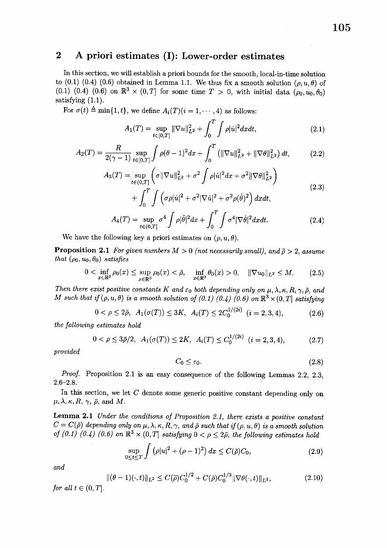
$2A$ priori estimates (I): Lower-order estimatesIn this section, we will establish a priori bounds for the smooth, local-in-time solution

to (0.1) (0.4) (0.6) obtained in Lemma 1.1. We thus fix a smooth solution $(\rho, u, \theta)$ of(0.1) (0.4) (0.6) on $\mathbb{R}^{3}\cross(0, T] for some time T>0, with$ initial $data (\rho_{0}, u_{0}, \theta_{0})$

satisfying (1. 1).For $\sigma(t)=\Delta\min\{1, t\}$ , we define $A_{i}(T)(i=1, \cdots, 4)$ as follows:

$A_{1}(T)= \sup_{t\in[0,T]}\Vert\nabla u\Vert_{L^{2}}^{2}+\int_{0}^{T}\int\rho|\dot{u}|^{2}dxdt$, (2.1)

$A_{2}(T)= \frac{R}{2(\gamma-1)}\sup_{t\in[0,T]}\int\rho(\theta-1)^{2}dx+\int_{0}^{T}(\Vert\nabla u\Vert_{L^{2}}^{2}+\Vert\nabla\theta\Vert_{L^{2}}^{2})dt$ , (2.2)

$A_{3}(T)= \sup_{t\in(0,T]}(\sigma\Vert\nabla u\Vert_{L^{2}}^{2}+\sigma^{2}\int\rho|\dot{u}|^{2}dx+\sigma^{2}\Vert\nabla\theta\Vert_{L^{2}}^{2})$

(2.3)$+ \int_{0}^{T}\int(\sigma\rho|\dot{u}|^{2}+\sigma^{2}|\nabla\dot{u}|^{2}+\sigma^{2}\rho(\dot{\theta})^{2})dxdt,$

$A_{4}(T)= \sup_{t\in(0,T]}\sigma^{4}\int\rho|\dot{\theta}|^{2}dx+\int_{0}^{T}\int\sigma^{4}|\nabla\dot{\theta}|^{2}dxdt$ . (2.4)

We have the following key a priori estimates on $(\rho, u, \theta)$ .Proposition 2.1 For given numbers $M>0$ (not necessarily small), and $\overline{\rho}>2$ , assumethat $(\rho_{0}, u_{0}, \theta_{0})$ satisfies

$0< \inf_{x\in \mathbb{R}^{3}}\rho_{0}(x)\leq\sup_{x\in \mathbb{R}^{3}}\rho_{0}(x)<\overline{\rho}, \inf_{x\in \mathbb{R}^{3}}\theta_{0}(x)>0, \Vert\nabla u_{0}\Vert_{L^{2}}\leq M$. (2.5)

Then there exist positive constants $K$ and $\epsilon_{0}$ both depending only on $\mu,$$\lambda,$

$\kappa,$ $R,$ $\gamma,\overline{\rho}$ , and$M$ such that if $(\rho, u, \theta)$ is a smooth solution of (0.1) $(o.4)(0.6)$ on $\mathbb{R}^{3}\cross(0, T]$ satisfying

$0<\rho\leq 2\overline{\rho}, A_{1}(\sigma(T))\leq 3K, A_{i}(T)\leq 2C_{0}^{1/(2i)}(i=2,3,4)$, (2.6)

the following estimates hold

$0<\rho\leq 3\overline{\rho}/2, A_{1}(\sigma(T))\leq 2K, A_{i}(T)\leq C_{0}^{1/(2i)}(i=2,3,4)$ , (2.7)

provided$C_{0}\leq\epsilon_{0}$ . (2.8)

Pmof. Proposition 2.1 is an easy consequence of the following Lemmas 2.2, 2.3,2.6-2.8.

In this section, we let $C$ denote some generic positive constant depending only on$\mu,$

$\lambda,$$\kappa,$ $R,$ $\gamma,\overline{\rho}$ , and $M.$

Lemma 2.1 Under the conditions of Proposition 2.1, there exists a positive constant$C=C(\overline{\rho})$ depending only on $\mu,$

$\lambda,$$\kappa,$ $R,$ $\gamma$ , and $\overline{\rho}$ such that if $(\rho, u, \theta)$ is a smooth solution

of (0.1) (0.4) (0.6) on $\mathbb{R}^{3}\cross(0, T]$ satisfying $0<\rho\leq 2\overline{\rho}$ , the following estimates hold

$\sup_{0\leq t\leq T}\int(\rho|u|^{2}+(\rho-1)^{2})dx\leq C(\overline{\rho})C_{0}$ , (2.9)

and$\Vert(\theta-1)(\cdot, t)\Vert_{L^{2}}\leq C(\overline{\rho})C_{0}^{1/2}+C(\overline{\rho})C_{0}^{1/3}\Vert\nabla\theta(\cdot, t)\Vert_{L^{2}}$ , (2.10)

for all $t\in(O, T].$

105

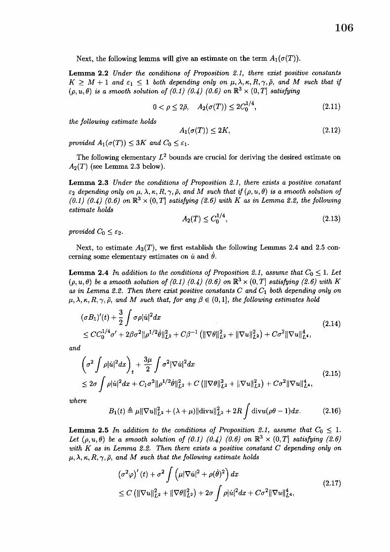
Next, the following lemma will give an estimate on the term $A_{1}(\sigma(T))$ .

Lemma 2.2 Under the conditions of Proposition 2.1, there exist positive constants$K\geq M+1$ and $\epsilon_{1}\leq 1$ both depending only on $\mu,$

$\lambda,$$\kappa,$ $R,$ $\gamma,\overline{\rho}$ , and $M$ such that if

$(\rho, u, \theta)$ is a smooth solution of (0.1) $(o.4)(0.6)$ on $\mathbb{R}^{3}\cross(0, T]$ satisfying

$0<\rho\leq 2\overline{\rho}, A_{2}(\sigma(T))\leq 2C_{0}^{1/4}$ , (2.11)

the following estimate holds$A_{1}(\sigma(T))\leq 2K$ , (2.12)

provided $A_{1}(\sigma(T))\leq 3K$ and $C_{0}\leq\epsilon_{1}.$

The following elementary $L^{2}$ bounds are crucial for deriving the desired estimate on$A_{2}(T)$ (see Lemma 2.3 below).

Lemma 2.3 Under the conditions of Proposition 2.1, there exists a positive constant$\epsilon_{2}$ depending only on $\mu,$

$\lambda,$$\kappa,$ $R,$ $\gamma,\overline{\rho}$ , and $M$ such that if $(\rho, u, \theta)$ is a smooth solution of

(0.1) (0.4) (0.6) on $\mathbb{R}^{3}\cross(0, T]$ satisfying $(2.6)$ with $K$ as in Lemma 2.2, the followingestimate holds

$A_{2}(T)\leq C_{0}^{1/4}$ , (2.13)

provided $C_{0}\leq\epsilon_{2}.$

Next, to estimate $A_{3}(T)$ , we first establish the following Lemmas 2.4 and 2.5 con-cerning some elementary estimates on $\dot{u}$ and $\dot{\theta}.$

Lemma 2.4 In addition to the conditions of Proposition 2.1, assume that $C_{0}\leq 1$ . Let$(\rho, u, \theta)$ be a smooth solution of (0.1) (0.4) (0.6) on $\mathbb{R}^{3}\cross(0, T]$ satisfying $(2.6)$ with $K$

as in Lemma 2.2. Then there exist positive constants $C$ and $C_{1}$ both depending only on$\mu,$

$\lambda,$$\kappa,$ $R,$ $\gamma,\overline{\rho}$, and $M$ such that, for any $\beta\in(0,1]$ , the following estimates hold

$( \sigma B_{1})’(t)+\frac{3}{2}\int\sigma\rho|\dot{u}|^{2}dx$

(2.14)$\leq CC_{0}^{1/4}\sigma’+2\beta\sigma^{2}\Vert\rho^{1/2}\dot{\theta}\Vert_{L^{2}}^{2}+C\beta^{-1}(\Vert\nabla\theta\Vert_{L^{2}}^{2}+\Vert\nabla u\Vert_{L^{2}}^{2})+C\sigma^{2}\Vert\nabla u\Vert_{L^{4}}^{4},$

and

$( \sigma^{2}\int\rho|\dot{u}|^{2}dx)_{t}+\frac{3\mu}{2}\int\sigma^{2}|\nabla\dot{u}|^{2}dx$

(2.15)$\leq 2\sigma\int\rho|\dot{u}|^{2}dx+C_{1}\sigma^{2}\Vert\rho^{1/2}\dot{\theta}\Vert_{L^{2}}^{2}+C(\Vert\nabla\theta\Vert_{L^{2}}^{2}+\Vert\nabla u\Vert_{L^{2}}^{2})+C\sigma^{2}\Vert$Vu $\Vert_{L^{4}}^{4},$

where$B_{1}(t)= \Delta\mu\Vert\nabla u\Vert_{L^{2}}^{2}+(\lambda+\mu)\Vert divu\Vert_{L^{2}}^{2}+2R\int divu(\rho\theta-1)dx$ . (2.16)

Lemma 2.5 In addition to the conditions of Proposition 2.1, assume that $C_{0}\leq 1.$

Let $(\rho, u, \theta)$ be a smooth solution of (0.1) $(o.4)(0.6)$ on $\mathbb{R}^{3}\cross(0, T]$ satisfying $(2.6)$

with $K$ as in Lemma 2.2. Then there exists a positive constant $C$ depending only on$\mu,$

$\lambda,$$\kappa,$ $R,$ $\gamma,\overline{\rho}$, and $M$ such that the following estimate holds

$( \sigma^{2}\varphi)’(t)+\sigma^{2}\int(\mu|\nabla\dot{u}|^{2}+\rho(\dot{\theta})^{2})dx$

(2.17)$\leq C(\Vert\nabla u\Vert_{L^{2}}^{2}+\Vert\nabla\theta\Vert_{L^{2}}^{2})+2\sigma\int\rho|\dot{u}|^{2}dx+C\sigma^{2}\Vert\nabla u\Vert_{L^{4}}^{4},$

106

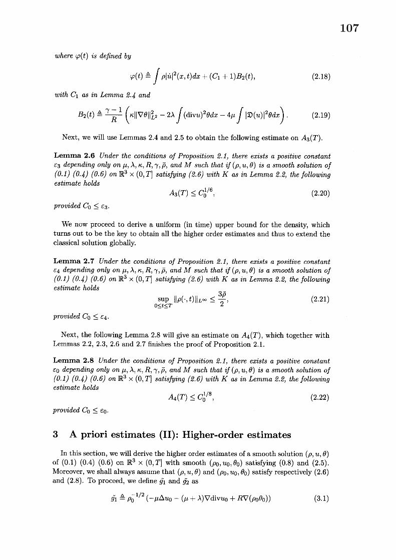
where $\varphi(t)$ is defined by

$\varphi(t)=\Delta\int\rho|\dot{u}|^{2}(x, t)dx+(C_{1}+1)B_{2}(t)$ , (2.18)

with $C_{1}$ as in Lemma 2.4 and

$B_{2}(t)= \Delta\frac{\gamma-1}{R}(\kappa\Vert\nabla\theta\Vert_{L^{2}}^{2}-2\lambda\int(divu)^{2}\theta dx-4\mu\int|\mathfrak{D}(u)|^{2}\theta dx)$ . (2.19)

Next, we will use Lemmas 2.4 and 2.5 to obtain the following estimate on $A_{3}(T)$ .

Lemma 2.6 Under the conditions of Proposition 2.1, there exists a positive constant$\epsilon_{3}$ depending only on $\mu,$

$\lambda,$$\kappa,$ $R,$ $\gamma,\overline{\rho}$ , and $M$ such that if $(\rho, u, \theta)$ is a smooth solution of

(0.1) $(o.4)(0.6)$ on $\mathbb{R}^{3}\cross(0, T]$ satisfying $(2.6)$ with $K$ as in Lemma 2.2, the followingestimate holds

$A_{3}(T)\leq C_{0}^{1/6}$ , (2.20)

provided $C_{0}\leq\epsilon_{3}.$

We now proceed to derive a uniform (in time) upper bound for the density, whichtums out to be the key to obtain all the higher order estimates and thus to extend theclassical solution globally.

Lemma 2.7 Under the conditions of Proposition 2.1, there exists a positive constant$\epsilon_{4}$ depending only on $\mu,$

$\lambda,$$\kappa,$ $R,$ $\gamma,\overline{\rho}$ , and $M$ such that if $(\rho, u, \theta)$ is a smooth solution of

(0.1) (0.4) (0.6) on $\mathbb{R}^{3}\cross(0, T]$ satisfying $(2.6)$ with $K$ as in Lemma 2.2, the followingestimate holds

$\sup_{0\leq t\leq T}\Vert\rho(\cdot, t)\Vert_{L^{\infty}}\leq\frac{3\overline{\rho}}{2}$ , (2.21)

provided $C_{0}\leq\epsilon_{4}.$

Next, the following Lemma 2.8 will give an estimate on $A_{4}(T)$ , which together withLemmas 2.2, 2.3, 2.6 and 2.7 finishes the proof of Proposition 2.1.

Lemma 2.8 Under the conditions of Proposition 2.1, there exists a positive constant$\epsilon_{0}$ depending only on $\mu,$

$\lambda,$$\kappa,$ $R,$ $\gamma,\overline{\rho}$, and $M$ such that if $(\rho, u, \theta)$ is a smooth solution of

(0.1) (0.4) (0.6) on $\mathbb{R}^{3}\cross(0, T]$ satisfying $(2.6)$ with $K$ as in Lemma 2.2, the followingestimate holds

$A_{4}(T)\leq C_{0}^{1/8}$ , (2.22)

provided $C_{0}\leq\epsilon_{0}.$

3 $A$ priori estimates (II): Higher-order estimates

In this section, we will derive the higher order estimates of a smooth solution $(\rho, u, \theta)$

of (0.1) (0.4) (0.6) on $\mathbb{R}^{3}\cross(0, T] with$ smooth $(\rho_{0}, u_{0}, \theta_{0})$ satisfying (0.8) and (2.5).Moreover, we shall always assume that $(\rho, u, \theta)$ and $(\rho 0, u_{0}, \theta_{0})$ satisfy respectively (2.6)and (2.8). To proceed, we define $\tilde{g}_{1}$ and $\tilde{g}_{2}$ as

$\tilde{g}_{1}=\Delta\rho_{0}^{1/2}(-\mu\triangle u_{0}-(\mu+\lambda)\nabla divu_{0}+R\nabla(\rho_{0}\theta_{0}))$ (3.1)

107

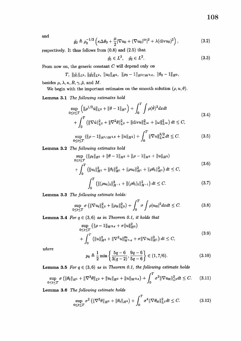
and$\tilde{g}_{2}=\Delta\rho_{0}^{-1/2}(\kappa\Delta\theta_{0}+\frac{\mu}{2}|\nabla u_{0}+(\nabla u_{0})^{tr}|^{2}+\lambda(divu_{0})^{2})$ , (3.2)

respectively. It thus follows from (0.8) and (2.5) that$\tilde{g}_{1}\in L^{2}, \tilde{g}_{2}\in L^{2}$. (3.3)

From now on, the generic constant $C$ will depend only on$T, \Vert\tilde{g}_{1}\Vert_{L^{2}}, \Vert\tilde{g}_{2}\Vert_{L^{2}}, \Vert u_{0}\Vert_{H^{2}}, \Vert\rho 0-1\Vert_{H^{2}\cap W^{2,q}}, \Vert\theta_{0}-1\Vert_{H^{2}},$

besides $\mu,$$\lambda,$

$\kappa,$ $R,$ $\gamma,\overline{\rho}$ , and $M.$

We begin with the important estimates on the smooth solution $(\rho, u, \theta)$ .

Lemma 3.1 The following estimates hold

$\sup_{0\leq t\leq T}(\Vert\rho^{1/2}\dot{u}\Vert_{L^{2}}+\Vert\theta-1\Vert_{H^{1}})+\int_{0}^{T}\int\rho(\dot{\theta})^{2}dxdt$

(3.4)$+ \int_{0}^{T}$ $(\Vert\nabla\dot{u}\Vert_{L^{2}}^{2}+\Vert\nabla^{2}\theta\Vert_{L^{2}}^{2}+\Vert$ divu $\Vert_{L^{\infty}}^{2}+\Vert\omega\Vert_{L^{\infty}}^{2})dt\leq C,$

$\sup_{0\leq t\leq T}(\Vert\rho-1\Vert_{H^{1}\cap W^{1,6}}+\Vert u\Vert_{H^{2}})+\int_{0}^{T}\Vert\nabla u\Vert_{L\infty}^{3/2}dt\leq C$. (3.5)

Lemma 3.2 The following estimates hold

$\sup_{0\leq t\leq T}(\Vert\rho_{t}\Vert_{H^{1}}+\Vert\theta-1\Vert_{H^{2}}+\Vert\rho-1\Vert_{H^{2}}+\Vert u\Vert_{H^{2}})$

$+ \int_{0}^{T}(\Vert u_{t}\Vert_{H^{1}}^{2}+\Vert\theta_{t}\Vert_{H^{1}}^{2}+\Vert\rho u_{t}\Vert_{H^{1}}^{2}+\Vert\rho\theta_{t}\Vert_{H^{1}}^{2})dt\leq C,$

(3.6)

$\int_{0}^{T}(\Vert(\rho u_{t})_{t}\Vert_{H^{-1}}^{2}+\Vert(\rho\theta_{t})_{t}\Vert_{H^{-1}}^{2})dt\leq C$. (3.7)

Lemma 3.3 The following estimate holds:

$\sup_{0\leq t\leq T}\sigma(\Vert\nabla u_{t}\Vert_{L^{2}}^{2}+\Vert\rho_{tt}\Vert_{L^{2}}^{2})+\int_{0}^{T}\sigma\int\rho|u_{tt}|^{2}dxdt\leq C$. (3.8)

Lemma 3.4 For $q\in(3,6)$ as in Theorem 0.1, it holds that

$\sup_{0\leq t\leq T}(\Vert\rho-1\Vert_{W^{2,q}}+\sigma\Vert u\Vert_{H^{3}}^{2})$

$+ \int_{0}^{T}(\Vert u\Vert_{H^{3}}^{2}+\Vert\nabla^{2}u\Vert_{W^{1,q}}^{p0}+\sigma\Vert\nabla u_{t}\Vert_{H^{1}}^{2})dt\leq C,$

(3.9)

where$p_{0}= \Delta\frac{1}{2}\min\{\frac{5q-6}{3(q-2)}, \frac{9q-6}{5q-6}\}\in(1,7/6)$ . (3.10)

Lemma 3.5 For $q\in(3,6)$ as in Theorem 0.1, the following estimate holds

$\sup_{0\leq t\leq T}\sigma(\Vert\theta_{t}\Vert_{H^{1}}+\Vert\nabla^{3}\theta\Vert_{L^{2}}+\Vert u_{t}\Vert_{H^{2}}+\Vert u\Vert_{W^{3,q}})+\int_{0}^{T}\sigma^{2}\Vert\nabla u_{tt}\Vert_{L^{2}}^{2}dt\leq C$. (3.11)

Lemma 3.6 The following estimate holds

$\sup_{0\leq t\leq T}\sigma^{2}(\Vert\nabla^{2}\theta\Vert_{H^{2}}+\Vert\theta_{t}\Vert_{H^{2}})+\int_{0}^{T}\sigma^{4}\Vert\nabla\theta_{tt}\Vert_{L^{2}}^{2}dt\leq C$. (3.12)

108

4 Proofs of Theorems 0.1 and 0.2

With all the a priori estimates in Sections 2 and 3 at hand, we are ready to provethe main results of this paper in this section.

Proposition 4.1 For given numbers $M>0$ (not necessarily small), $\overline{\rho}>2$ , assumethat $(\rho_{0}, u_{0}, \theta_{0})$ satisfies (1.1), (2.5), and (2.8). Then there exists a unique classical so-lution $(\rho, u, \theta)$ of $(0.1)(0.4)(0.6)$ in $\mathbb{R}^{3}\cross(0, \infty)$ satisfying $(1.3)-(1.5)$ with $T_{0}$ replacedby any $T\in(0, \infty)$ . Moreover, (2.9), (2.6) hold for any $T\in(O, \infty)$ .

Pmof of Theorem 0.1. Let $(\rho_{0}, u_{0}, \theta_{0})$ satisfying $(0.8)-(0.11)$ be initial data as de-scribed in Theorem 0.1. Assume that $C_{0}$ satisfies (0.12), where

$\epsilon=\epsilon_{0}\Delta/2$ , (4.1)

with $\epsilon_{0}$ as in Proposition 2.1. For constants

$\delta, \eta\in(0, \min\{1,\overline{\rho}-\sup_{x\in \mathbb{R}^{3}}\rho_{0}(x)\})$, (4.2)

we define$\rho_{0}^{\delta,\eta}=\Delta\frac{j_{\delta}*\rho_{0}+\eta}{1+\eta}, u_{0}^{\delta,\eta}=\triangle j_{\delta}*u_{0}, \theta_{0}^{\delta,\eta}=\triangle\frac{j_{\delta}*\theta_{0}+\eta}{1+\eta}$ , (4.3)

where $j_{\delta}$ is the standard mollifying kernel of width $\delta$. Then, $(\rho_{0}^{\delta,\eta}, u_{0}^{\delta,\eta}, \theta_{0}^{\delta,\eta})$ satisfies

$\{\begin{array}{ll}(\rho_{0}^{\delta,\eta}-1, u_{0}^{\delta,\eta}, \theta_{0}^{\delta,\eta}-1)\in H^{\infty}, \frac{\eta}{1+\eta}\leq\rho_{0}^{\delta,\eta}\leq\frac{\overline{\rho}+\eta}{1+\eta}<\overline{\rho}, \theta_{0}^{\delta,\eta}\geq\frac{\eta}{\overline{\rho}+\eta}, \Vert\nabla u_{0}^{\delta,\eta}\Vert_{L^{2}}\leq M,\end{array}$ (4.4)

and

$\{\begin{array}{l}\lim_{\delta+\etaarrow 0}(\Vert\rho_{0}^{\delta,\eta}-\rho 0\Vert_{H^{2}\cap W^{2,q}}+\Vert u_{0}^{\delta,\eta}-u_{0}\Vert_{H^{2}}+\Vert\theta_{0}^{\delta,\eta}-\theta_{0}\Vert_{H^{2}})=0,\Vert\nabla(\rho_{0}^{\delta,\eta}, u_{0}^{\delta,\eta}, \theta_{0}^{\delta,\eta})\Vert_{H^{1}}\leq\Vert\nabla(\rho_{0}, u_{0}, \theta_{0})\Vert_{H^{1}}, \Vert\nabla\rho_{0}^{\delta,\eta}\Vert_{W^{1,q}}\leq\Vert\nabla\rho_{0}\Vert_{W^{1,q}},\end{array}$ (4.5)

due to (0.8) and (0.9). Moreover, the initial norm $C_{0}^{\delta,\eta}$ for $(\rho_{0}^{\delta,\eta}, u_{0}^{\delta,\eta}, \theta_{0}^{\delta,\eta})$, i.e., the righthand side of (0.7) with $(\rho_{0}, u_{0}, \theta_{0})$ replaced by $(\rho_{0}^{\delta,\eta}, u_{0}^{\delta,\eta}, \theta_{0}^{\delta,\eta})$ , satisfies

$\lim_{\etaarrow 0}\lim_{\deltaarrow 0}C_{0}^{\delta,\eta}=C_{0}.$

Therefore, there exists an$\eta_{0}\in(0, \min\{1,\overline{\rho}-\sup_{x\in \mathbb{R}^{3}}\rho_{0}(x)\})$ such that, for any $\eta\in(0, \eta_{0})$ ,

we can find some $\delta_{0}(\eta)>0$ such that

$C_{0}^{\delta,\eta}\leq C_{0}+\epsilon 0/2\leq\epsilon_{0}$ , (4.6)

provided that$0<\eta\leq\eta_{0}, 0<\delta\leq\delta_{0}(\eta)$ . (4.7)

We assume that $\delta,$$\eta$ satisfy (4.7). Proposition 4.1 together with (4.6) and (4.4) thus

yields that there exists a smooth solution $(\rho^{\delta,\eta}, u^{\delta,\eta}, \theta^{\delta,\eta})$ of (0.1) (0.4) (0.6) with initialdata $(\rho_{0}^{\delta,\eta}, u_{0}^{\delta,\eta}, \theta_{0}^{\delta,\eta})$ on $\mathbb{R}^{3}\cross[0, T]$ for all $T>0$ . Moreover, (2.9) and (2.6) both holdwith $(\rho, u, \theta)$ being replaced by $(\rho^{\delta,\eta}, u^{\delta,\eta}, \theta^{\delta,\eta})$ .

109

Next, for the initial data $(\rho_{0}^{\delta,\eta}, u_{0}^{\delta,\eta}, \theta_{0}^{\delta,\eta})$, the $\tilde{g}_{1}$ in (3.1) in fact is

$\tilde{g}_{1}^{\Delta}=(\rho_{0}^{\delta,\eta})^{-1/2}(-\mu\Delta u_{0}^{\delta,\eta}-(\mu+\lambda)\nabla divu_{0}^{\delta,\eta}+R\nabla(\rho_{0}^{\delta,\eta}\theta_{0}^{\delta,\eta}))$

$=(\rho_{0}^{\delta,\eta})^{-1/2}(j_{\delta}*\rho_{0})^{1/2}g_{1}+(\rho_{0}^{\delta,\eta})^{-1/2}(j_{\delta}*(\sqrt{\rho 0}g_{1})-\sqrt{j_{\delta}*\rho 0}g_{1})$

(4.8)$+R(\rho_{0}^{\delta,\eta})^{-1/2}\nabla(j_{\delta}*(\rho_{0}\theta_{0})-(1+\eta)^{-2}(j_{\delta}*\rho_{0})(j_{\delta}*\theta_{0}))$

$+R\eta(1+\eta)^{-2}(\rho_{0}^{\delta,\eta})^{-1/2}\nabla(\rho_{0}^{\delta,\eta}+\theta_{0}^{\delta,\eta})$,

where in the second equality we have used (0.10). Similarly, the $\tilde{g}_{2}$ in (3.2) is

$\tilde{g}_{2^{\Delta}}=(\rho_{0}^{\delta,\eta})^{-1/2}(\kappa\triangle\theta_{0}^{\delta,\eta}+\frac{\mu}{2}|\nabla u_{0}^{\delta,\eta}+(\nabla u_{0}^{\delta,\eta})^{tr}|^{2}+\lambda(divu_{0}^{\delta,\eta})^{2})$

$=(\rho_{0}^{\delta,\eta})^{-1/2}(j_{\delta}*\rho_{0})^{1/2}g_{2}+(\rho_{0}^{\delta,\eta})^{-1/2}(j_{\delta}*(\sqrt{\rho 0}g_{2})-\sqrt{j_{\delta}*\rho 0}g_{2})$

(4.9)$- \frac{\mu}{2}(\rho_{0}^{\delta,\eta})^{-1/2}(j_{\delta}*(|\nabla u0+(\nabla uo)^{tr}|^{2})-|\nabla(j_{\delta}*u_{0})+(\nabla(j_{\delta}*u_{0}))^{tr}|^{2})$

$-\lambda(\rho_{0}^{\delta,\eta})^{-1/2}(j_{\delta}*((divu_{0})^{2})-(div(j_{\delta}*u_{0}))^{2})$ ,

due to (0.11). Since $g_{1},$$g_{2}\in L^{2}$ , one deduces from (4.8), (4.9), (4.4), (4.5), and (0.8)

that there exists some positive constant $C$ independent of $\delta$ and $\eta$ such that

$\{\begin{array}{l}\Vert\tilde{g}_{1}\Vert_{L^{2}}\leq(1+\eta)^{1/2}\Vert g_{1}\Vert_{L^{2}}+C\eta^{-1/2}m_{1}(\delta)+C\sqrt{\eta},\Vert\tilde{g}_{2}\Vert_{L^{2}}\leq(1+\eta)^{1/2}\Vert g_{2}\Vert_{L^{2}}+C\eta^{-1/2}m_{2}(\delta) ,\end{array}$ (4.10)

with $0\leq m_{i}(\delta)arrow 0(i=1,2)$ ae $\deltaarrow 0$ . Hence, for any $0<\eta<0$ , there exists some$0<\delta_{1}(\eta)\leq\delta_{0}(\eta)$ such that

$m_{1}(\delta)+m_{2}(\delta)<\eta$ , (4.11)

for any $0<\delta<\delta_{1}(\eta)$ . We thus obtain from (4.10) and (4.11) that there exists somepositive constant $C$ independent of $\delta$ and $\eta$ such that

$\Vert\tilde{g}_{1}\Vert_{L^{2}}+\Vert\tilde{g}_{2}\Vert_{L^{2}}\leq 2\Vert g_{1}\Vert_{L^{2}}+2\Vert g_{2}\Vert_{L^{2}}+C$, (4.12)

provided that$0<\eta<\eta 0, 0<\delta<\delta_{1}(\eta)$ . (4.13)

Now, we assume that $\eta,$$\delta$ satisfy (4.13). It thus follows from (4.6), Proposition

2.1, (4.5), (4.12), and Lemmas 3.1-3.6 that for any $T>0$ , there exists some positiveconstant $C$ independent of $\delta$ and $\eta$ such that (2.9), (2.6), (3.6), (3.7), (3.9), (3.11),and (3.12) hold for $(\rho^{\delta,\eta}, u^{\delta,\eta}, \theta^{\delta,\eta})$ . Then passing to the limit first $\deltaarrow 0$ , then $\etaarrow 0,$

together with standard arguments yields that there exists a solution $(\rho, u, \theta)$ of (0.1)(0.4) (0.6) on $\mathbb{R}^{3}\cross(0, T] for all T>0, such that (\rho, u, \theta)$ satisfies (2.9), (2.6), (3.6),(3.7), (3.9), (3.11) and (3.12). Hence, $(\rho, u, \theta)$ satisfies (0.13), $(0.14)_{2},$ $(0.14)_{3}$ , and

$\rho-1\in L^{\infty}(0, T;H^{2}\cap W^{2,q}) , (u, \theta-1)\in L^{\infty}(0, T;H^{2})$ . (4.14)

Moreover, $(0.1)$ holds in $\mathcal{D}’(\mathbb{R}^{3}\cross(0, T))$ .Next, to finish the existence part of Theorem 0.1, it remains to prove

$\rho-1\in C([0, T];H^{2}\cap W^{2,q}) , u, \theta-1\in C([0, T];H^{2})$ . (4.15)

It follows from (3.6) and (4.14) that

$\rho-1\in C([0, T];H^{1}\cap W^{1,\infty})\cap C([0, T];H^{2}\cap W^{2,q} - weak)$ , (4.16)

110

and for all $r\in[2,6)$ ,$u, \theta-1\in C([0, T];H^{1}\cap W^{1,r})$ . (4.17)

Since (0.1) holds in $\mathcal{D}’(\mathbb{R}^{3}\cross(0, T))$ for all $T\in(0, \infty)$ , one derives from [15, Lemma2.3] that, for $j_{\nu}(x)$ being the standard mollifying kernel of width $v,$ $\rho^{\nu}=\Delta\rho*j_{\nu}$ satisfies

$(\triangle\rho^{\nu})_{t}+div(u\Delta\rho^{\nu})=-div(\rho\triangle u)*j_{\nu}-2div(\partial_{i}\rho\cdot\partial_{i}u)*j_{\nu}+R_{\nu}$ , (4.18)

where $R_{\nu}$ satisfies

$\int_{0}^{T}\Vert R_{\nu}\Vert_{L^{2}\cap L^{q}}^{3/2}dt\leq C\int_{0}^{T}\Vert u\Vert_{W^{1\infty}}^{3/2},\Vert\Delta\rho\Vert_{L^{2}\cap L^{q}}^{3/2}dt\leq C$, (4.19)

due to (3.5), (3.6), and (3.9). Multiplying (4.18) by $q|\Delta\rho^{\nu}|^{q-2}\triangle\rho^{\nu}$ , we obtain afterintegration by parts that

$(\Vert\Delta\rho^{\nu}\Vert_{Lq}^{q})’(t)$

$=(1-q) \int|\triangle\rho^{\nu}|^{q}divudx-q\int(div(\rho\triangle u)*j_{\nu})|\triangle\rho^{\nu}|^{q-2}\triangle\rho^{\nu}dx$

$-2q \int(div(\partial_{i}\rho\cdot\partial_{i}u)*j_{\nu})|\triangle\rho^{\nu}|^{q-2}\triangle\rho^{v}dx+q\int R_{\nu}|\triangle\rho^{\nu}|^{q-2}\triangle\rho^{\nu}dx,$

which together with (3.6), (3.9), and (4.19) yields that, for $p_{0}$ as in (3.10),

$\sup_{t\in[0,T]}\Vert\triangle\rho^{\nu}\Vert_{Lq}+\int_{0}^{T}|(\Vert\Delta\rho^{\nu}\Vert_{L^{q}}^{q})’(t)|^{po}dt$

$\leq C+C\int_{0}^{T}(\Vert\nabla u\Vert_{W^{2,q}}^{p0}+\Vert R_{\nu}\Vert_{L^{2}\cap L^{q}}^{p0})dt$

$\leq C.$

This fact combining with the Ascoli-Arzela theorem thus leads to

$\Vert\triangle\rho^{\nu}(\cdot, t)\Vert_{Lq}arrow\Vert\Delta\rho(\cdot, t)\Vert_{Lq}$ in $C([O, T])$ , as $\nuarrow 0^{+}.$

In particular, we have$\Vert\nabla^{2}\rho(\cdot, t)\Vert_{Lq}\in C([O, T])$ . (4.20)

Similarly, one can obtain that

$\Vert\nabla^{2}\rho(\cdot, t)\Vert_{L^{2}}\in C([O, T])$ . (4.21)

Therefore, the continuity of $\nabla^{2}\rho$ in $L^{p}(p=2, q)$ , i.e.,

$\nabla^{2}\rho\in C([0, T];L^{2}\cap L^{q})$ , (4.22)

follows directly from (4.16), (4.20), and (4.21).It follows from (3.6) and (3.7) that

$\rho u_{t}, \rho\theta_{t}\in C([0, T];L^{2})$ , (4.23)

which together with (4.16), (4.17), and (4.22) gives

$u\in C([0, T];H^{2})$ . (4.24)

111

This fact combining with (4.23), (4.22), (4.17), and (3.6) leads to

$\theta-1\in C([0, T];H^{2})$ ,

which as well as (4.16), (4.22), and (4.24) leads to (4.15).Finally, since the proof of the uniqueness of $(\rho, u, \theta)$ is similar to that of [4, Theorem

1 $]$ , to finish the proof of Theorem 0.1, it remains to prove (0.15). We will only show

$\lim_{tarrow\infty}\Vert Vu\Vert_{L^{2}}=0$, (4.25)

since the other terms in (0.15) follow directly from (0.26). It follows from (2.6) that

$l^{\infty}|(\Vert\nabla u\Vert_{L^{2}}^{2})’(t)|dt$

$=2 \int_{1}^{\infty}|\int\partial_{j}u^{i}\partial_{j}u_{t}^{i}dx|dt$

$=2l^{\infty}| \int\partial_{j}u^{i}\partial_{j}(\dot{u}^{i}-u^{k}\partial_{k}u^{i})dx|dt$

$=2 \int_{1}^{\infty}|\int(\partial_{j}u^{i}\partial_{j}\dot{u}^{i}-\partial_{j}u^{i}\partial_{j}u^{k}\partial_{k}u^{i}-\partial_{j}u^{i}u^{k}\partial_{kj}u^{i})dx|dt$

$=l^{\infty}| \int(2\partial_{j}u^{i}\partial_{j}\dot{u}^{i}-2\partial_{j}u^{i}\partial_{j}u^{k}\partial_{k}u^{i}+|\nabla u|^{2}divu)dx|dt$

$\leq C\int_{1}^{\infty}(\Vert\nabla u\Vert_{L^{2}}\Vert\nabla\dot{u}\Vert_{L^{2}}+\Vert\nabla u\Vert_{L^{3}}^{3})dt$

$\leq C\int_{1}^{\infty}(\Vert\nabla\dot{u}\Vert_{L^{2}}^{2}+\Vert\nabla u\Vert_{L^{2}}^{2}+\Vert\nabla u\Vert_{L^{4}}^{4})dt$

$\leq C,$

which together with (2.6) implies (4.25). We finish the proof of Theorem 0.1.Pmof of Theorem 0.2. We will prove TheoremO.2in three steps.Step 1. Construction of approximate solutions. Let $(\rho_{0}, u_{0}, \theta_{0})$ satisfying (0.9) be

initial data as described in Theorem 0.2. Assume that $C_{0}$ satisfies (0.21) with $\epsilon$ as in(4.1). Let $\delta$ and $\eta$ be as in (4.2) and $j_{\delta}$ be the standard mollifier. We define

$\hat{\rho}_{0}^{\delta,\eta}=\Delta\frac{j_{\delta}*\rho 0+\eta}{1+\eta}, \hat{u}_{0}^{\delta,\eta}=\Delta j_{\delta}*u_{0}, \hat{\theta}_{0}^{\delta,\eta}=\Delta\frac{j_{\delta}*(\rho 0\theta_{0})+\eta}{j_{\delta}*\rho 0+\eta}$ . (4.26)

Then, $(\hat{\rho}_{0}^{\delta,\eta},\hat{u}_{0}^{\delta,\eta},\hat{\theta}_{0}^{\delta,\eta})$ satisfies

$\{\begin{array}{ll}(\hat{\rho}_{0}^{\delta,\eta}-1,\hat{u}_{0}^{\delta,\eta},\hat{\theta}_{0}^{\delta,\eta}-1)\in H^{\infty}, 0<\frac{\eta}{1+\eta}\leq\hat{\rho}_{0}^{\delta,\eta}\leq\frac{\overline{\rho}+\eta}{1+\eta}<\overline{\rho}, \hat{\theta}_{0}^{\delta,\eta}\geq\frac{\eta}{\overline{\rho}+\eta}>0, \Vert\nabla\hat{u}_{0}^{\delta,\eta}\Vert_{L^{2}}\leq M,\end{array}$ (4.27)

due to (0.9). Moreover, it follows from (0.9) and (0.21) that

$\lim_{\etaarrow 0}\lim_{\deltaarrow 0}(\Vert\hat{\rho}_{0}^{\delta,\eta}-\rho 0\Vert_{L^{2}}+\Vert\hat{u}_{0}^{\delta,\eta}-uo\Vert_{H^{1}}+\Vert\hat{\rho}_{0}^{\delta,\eta}\hat{\theta}_{0}^{\delta,\eta}-\rho 0\theta_{0}\Vert_{L^{2}})=0$ . (4.28)

We claim that the initial norm $\hat{C}_{0}^{\delta,\eta}$ for $(\hat{\rho}_{0}^{\delta,\eta},\hat{u}_{0}^{\delta,\eta},\hat{\theta}_{0}^{\delta,\eta})$ , i.e., the right hand side of (0.7)with $(\rho_{0}, u_{0}, \theta_{0})$ replaced by $(\hat{\rho}_{0}^{\delta,\eta},\hat{u}_{0}^{\delta,\eta},\hat{\theta}_{0}^{\delta,\eta})$, satisfies

lim $\lim\hat{C}_{0}^{\delta,\eta}\leq C_{0}$ , (4.29)$\etaarrow 0\deltaarrow 0$

112

which yields that there exists an $\hat{\eta}>0$ such that, for any $\eta\in(0,\hat{\eta})$ , there exists some$\hat{\delta}(\eta)>0$ such that

$\hat{C}_{0}^{\delta,\eta}\leq C_{0}+\epsilon 0/2\leq\epsilon_{0}$ , (4.30)

provided$0<\eta\leq\hat{\eta}, 0<\delta\leq\hat{\delta}(\eta)$ . (4.31)

We assume that $\delta,$$\eta$ always satisfy (4.31). Proposition 4.1 as well ae (4.27) and (4.30)

thus yields that there exists a smooth solution $(\hat{\rho}^{\delta,\eta},\hat{u}^{\delta,\eta},\hat{\theta}^{\delta,\eta})$ of (0.1) (0.4) (0.6) withinitial data $(\hat{\rho}_{0}^{\delta,\eta},\hat{u}_{0}^{\delta,\eta},\hat{\theta}_{0}^{\delta,\eta})$ on $\mathbb{R}^{3}\cross[0, T]$ for all $T>0$ . Moreover, for any $T>0,$$(\hat{\rho}^{\delta,\eta},\hat{u}^{\delta,\eta},\hat{\theta}^{\delta,\eta})$ satisfies (2.9), (2.6) with $(\rho, u, \theta)$ replaced by $(\hat{\rho}^{\delta,\eta},\hat{u}^{\delta,\eta},\hat{\theta}^{\delta,\eta})$ .

It remains to prove (4.29). In fact, we only have to show

$\etaarrow 0\deltaarrow 0hm\lim\int\hat{\rho}_{0}^{\delta,\eta}(\hat{\theta}_{0}^{\delta,\eta}-\log\hat{\theta}_{0}^{\delta,\eta}-1)dx\leq\int\rho_{0}(\theta_{0}-\log\theta_{0}-1)dx$ , (4.32)

since the other terms in (4.29) can be proved in a similar and even simpler way. Noticingthat

$\hat{\rho}_{0}^{\delta,\eta}(\hat{\theta}_{0}^{\delta,\eta}-\log\hat{\theta}_{0}^{\delta,\eta}-1)$

$= \hat{\rho}_{0}^{\delta,\eta}(\hat{\theta}_{0}^{\delta,\eta}-1)^{2}\int_{0}^{1}\frac{\alpha}{\alpha(\hat{\theta}_{0}^{\delta,\eta}-1)+1}d\alpha$

$= \frac{(j_{\delta}*(\rho_{0}\theta_{0}-\rho_{0}))^{2}}{1+\eta}\int_{0}^{1}\frac{\alpha}{\alpha(j_{\delta}*(\rho_{0}\theta_{0})-j_{\delta}*\rho_{0})+j_{\delta}*\rho 0+\eta}d\alpha$

$\in[0, \eta^{-1}(j_{\delta}*(\rho_{0}\theta_{0}-\rho_{0}))^{2}],$

we deduce from (4.28) and Lebesgue’s dominated convergence theorem that

$\lim_{\deltaarrow 0}\int\hat{\rho}_{0}^{\delta,\eta}(\hat{\theta}_{0}^{\delta,\eta}-\log\hat{\theta}_{0}^{\delta,\eta}-1)dx$

$= \int\frac{\rho_{0}+\eta}{1+\eta}(\frac{\rho_{0}\theta_{0}+\eta}{\rho_{0}+\eta}-\log\frac{\rho_{0}\theta_{0}+\eta}{\rho_{0}+\eta}-1)dx$

$=(1+ \eta)^{-1}\int_{(\rho 0\theta_{0}<1/2)\cup(\rho 0\theta_{0}>2)}(\rho_{0}\theta_{0}-\rho_{0}-(\rho_{0}+\eta)\log\frac{\rho_{0}\theta_{0}+\eta}{\rho_{0}+\eta})dx$ (4.33)

$+(1+ \eta)^{-1}\int_{(1/2\leq\rho_{0}\theta_{0}\leq 2)}(\rho 0+\eta)(\frac{\rho_{0}\theta_{0}+\eta}{\rho 0+\eta}-\log\frac{\rho_{0}\theta_{0}+\eta}{\rho 0+\eta}-1)dx$

$=\Delta(1+\eta)^{-1}I_{1}+(1+\eta)^{-1}I_{2},$

where we have used the following simple fact that, for $f\in L^{p}(1\leq p<\infty)$ ,

$\lim_{\deltaarrow 0}\Vert j_{\delta}*f-f\Vert_{L^{p}}=0,$ $\lim_{\deltaarrow 0}j_{\delta}*f(x)=f(x)$ , a.e. $x\in \mathbb{R}^{3}.$

It follows from (0.21) that

$|(\rho_{0}\theta_{0}<1/2)\cup(\rho_{0}\theta_{0}>2)|$

$\leq 4\int(\rho_{0}\theta_{0}-1)^{2}dx$

$\leq 8\int(\rho_{0}\theta_{0}-\rho_{0})^{2}dx+8\int(\rho 0-1)^{2}dx$

$\leq C,$

113

which combining with Lebesgue’s dominated convergence theorem yields

$I_{1}= \int_{(\rho 0\theta_{0}<1/2)\cup(\rho 0\theta_{0}>2)}(\rho_{0}\theta_{0}-\rho_{0}\log(\rho_{0}\theta_{0}+\eta)-\eta\log(\rho_{0}\theta_{0}+\eta))dx$

$+ \int_{(\rho 0\theta_{0}<1/2)\cup(\rho_{0}\theta_{0}>2)}((\rho 0+\eta)\log(\rho 0+\eta)-\rho_{0})dx$

$\leq\int_{(\rho 0\theta_{0}<1/2)\cup(\rho_{0}\theta_{0}>2)}(\rho_{0}\theta_{0}-\rho_{0}\log(\rho 0\theta_{0})-\eta\log\eta)dx$ (4.34)

$+ \int_{(\rho 0\theta_{0}<1/2)\cup(\rho 0\theta_{0}>2)}(\rho_{0}\log(\rho 0+\eta)+\eta\log(\rho 0+\eta)-\rho_{0})dx$

$arrow\int_{(\rho 0\theta_{0}<1/2)\cup(\rho 0\theta_{0}>2)}\rho_{0}(\theta_{0}-\log\theta_{0}-1)dx$ , a$s$ $\etaarrow 0.$

Noticing that

$( \rho 0+\eta)(\frac{\rho_{0}\theta_{0}+\eta}{\rho 0+\eta}-\log\frac{\rho_{0}\theta_{0}+\eta}{\rho 0+\eta}-1)$

$=( \rho_{0}\theta_{0}-\rho_{0})^{2}\int_{0}^{1}\frac{\alpha}{\alpha(\rho 0\theta_{0}-\rho_{0})+\rho 0+\eta}d\alpha$

$\in[0,2(\rho_{0}\theta_{0}-\rho_{0})^{2}],$

provided $\rho_{0}\theta_{0}\geq 1/2$ , we deduce from Lebesgue’s dominated convergence theorem that

$\lim_{\etaarrow 0}I_{2}=\int_{(1/2\leq\rho 0\theta_{0}\leq 2)}\rho_{0}(\theta_{0}-\log\theta_{0}-1)dx,$

which together with (4.33) and (4.34) gives (4.32).Step 2. Compactness results. For the approximate solutions $(\hat{\rho}^{\delta,\eta},\hat{u}^{\delta,\eta},\hat{\theta}^{\delta,\eta})$ obtained

in the previous step, we will pass to the limit first $\deltaarrow 0$ , then $\etaarrow 0$ and apply (2.6)to obtain the global existence of weak solutions. Since the two steps are similar, wewill only sketch the arguments for $\deltaarrow 0$ . Thus, we fix $\eta\in(0,\hat{\eta})$ and simply denote$(\hat{\rho}^{\delta,\eta},\hat{u}^{\delta,\eta},\hat{\theta}^{\delta,\eta})$ by $(\rho^{\delta}, u^{\delta}, \theta^{\delta})$ . For $R\in(0, \infty)$ , let $B_{R}(x_{0})=\Delta\{x\in \mathbb{R}^{3}||x-x_{0}|<R\}$

denote a ball centered at $x_{0}\in \mathbb{R}^{3}$ with radius $R$ . We claim that there exists someappropriate subsequence $\delta_{j}arrow 0$ of $\deltaarrow 0$ such that, for any $0<\tau<T<\infty$ and$0<R<\infty$ , we have

$\{\begin{array}{l}\theta^{\delta_{j}}-1arrow\theta-1 weakly in L^{2}(0, T;H^{1}(\mathbb{R}^{3})) ,u^{\delta_{j}}arrow u weakly star in L^{\infty}(0, T;H^{1}(\mathbb{R}^{3})) ,\end{array}$ (4.35)

$\{\begin{array}{ll}\rho^{\delta_{j}}-1arrow\rho-1 in C([0, T];L^{2}(\mathbb{R}^{3})- weak ) ,\rho^{\delta_{j}}-1arrow\rho-1 in C([0, T];H^{-1}(B_{R}(0))) ,\end{array}$ (4.36)

$\{\begin{array}{l}\rho^{\delta_{j}}u^{\delta_{j}}arrow\rho u, \rho^{\delta_{j}}(\theta^{\delta_{j}}-1)arrow\rho(\theta-1) in C([0, T];L^{2}(\mathbb{R}^{3})- weak ) ,\rho^{\delta_{j}}u^{\delta_{j}}arrow\rho u in C([0, T];H^{-1}(B_{R}(0))) ,\end{array}$ (4.37)

$\rho^{\delta_{j}}|u^{\delta_{j}}|^{2}arrow\rho|u|^{2}$ in $C([O, T];L^{3}- weak)$ , (4.38)

and

$\{\begin{array}{l}u^{\delta_{j}}arrow u, G^{\delta_{j}}arrow G, \omega^{\delta_{j}}arrow\omega, \nabla\theta^{\delta_{j}}arrow\nabla\theta in C([\tau, T];H^{1}(\mathbb{R}^{3})-weak ) ,u^{\delta_{j}}arrow u, G^{\delta_{j}}arrow G, \omega^{\delta_{j}}arrow\omega, \nabla\theta^{\delta_{j}}arrow\nabla\theta in C([\tau, T];L^{2}(B_{R}(0))) .\end{array}$ (4.39)

114

We thus write (0.1) in the weak forms for the approximate solutions $(\rho^{\delta}, u^{\delta}, \theta^{\delta})$ , thenlet $\delta=\delta_{j}$ and take appropriate limits. Standard arguments as well as $(4.35)-(4.39)$thus yield that the limit $(\rho, u, \theta)$ is a weak solution of (0.1) (0.4) (0.5) in the senseof Definition 0.1 and satisfies $(0.22)-(0.25)$ except $\rho-1\in C([O, \infty), L^{2})$ which in factcan be obtained by similar arguments leading to (4.22). In addition, the estimates$(0.27)-(0.29)$ follows direct from (2.9), (2.6), and $(4.35)-(4.39)$ .

It remains to prove $(4.36)-(4.39)$ since (4.35) is a direct consequence of (2.6). Itfollows from (2.9), (2.6), and $(0.1)_{1}$ that

$\sup \Vert\rho_{t}^{\delta}\Vert_{H^{-1}(\mathbb{R}^{3})}\leq C,$

$t\in[0,\infty)$

which as well as (2.6), [15, Lemma C.l], and the Aubin-Lions lemma yields that thereexists a subsequence of $\delta_{j}arrow 0$ , still denoted by $\delta_{j}$ , such that (4.36) holds. Moreover,one deduces that (extract a subsequence)

$\rho^{\delta_{j}}-1arrow\rho-1,$ $\nabla u^{\delta_{j}}arrow\nabla u$ weakly in $L^{4}(\mathbb{R}^{3}\cross(1, \infty))$ ,

with $\rho-1$ and $\nabla u$ satisfying

$\int_{1}^{\infty}(\Vert\rho-1\Vert_{L^{4}}^{4}+\Vert\nabla u\Vert_{L^{4}}^{4})dt\leq C$ . (4.40)

Then, simple calculations together with (2.6) yield that, for any $0<T<\infty$ , thereexists some $C(T)$ independent of $\delta$ and $\eta$ such that

$\Vert(\rho^{\delta}u^{\delta})_{t}\Vert_{L^{2}(0,T;H^{-1}(\mathbb{R}^{3}))}+\Vert(\rho^{\delta}\theta^{\delta})_{t}\Vert_{L^{2}(0,T;H^{-1}(\mathbb{R}^{3}))}\leq C(T)$ , (4.41)

which together with (2.6), (4.36), and (4.35) gives (4.37).Next, to prove (4.38), one deduces from (2.6) and $(0.1)_{1}$ that, for any $\zeta\in H^{1}(\mathbb{R}^{3})$ ,

$| \int(\rho^{\delta}|u^{\delta}|^{2})_{t}\zeta dx|$

$=|- \int div(\rho^{\delta}u^{\delta})|u^{\delta}|^{2}\zeta dx+2\int\rho^{\delta}u^{\delta}\cdot u_{t}^{\delta}\zeta dx|$

$=| \int\rho^{\delta}u^{\delta}\cdot\nabla(|u^{\delta}|^{2}\zeta)dx+2\int\rho^{\delta}u^{\delta}\cdot(\dot{u}^{\delta}-u^{\delta}\cdot\nabla u^{\delta})\zeta dx|$

$\leq C\int\rho^{\delta}|u^{\delta}|^{3}|\nabla\zeta|dx+C\int\rho^{\delta}|u^{\delta}|^{2}|\nabla u^{\delta}||\zeta|dx+C\int\rho^{\delta}|u^{\delta}||\dot{u}^{\delta}||\zeta|dx$

$\leq C\Vert u^{\delta}\Vert_{L^{6}}^{3}\Vert\nabla\zeta\Vert_{L^{2}}+C\Vert u^{\delta}\Vert_{L^{6}}^{2}\Vert\nabla u^{\delta}\Vert_{L^{2}}\Vert\zeta\Vert_{L^{6}}+C\Vert u^{\delta}\Vert_{L^{6}}\Vert(\rho^{\delta})^{1/2}\dot{u}^{\delta}\Vert_{L^{2}}\Vert\zeta\Vert_{L^{3}}$

$\leq C(\Vert\nabla u^{\delta}\Vert_{L^{2}}+\Vert(\rho^{\delta})^{1/2}\dot{u}^{\delta}\Vert_{L^{2}})\Vert\zeta\Vert_{H^{1}},$

which together with (2.6) gives

$\int_{0}^{\infty}\Vert(\rho^{\delta}|u^{\delta}|^{2})_{t}\Vert_{H}^{2_{-1}}dt\leq C$. (4.42)

It follows from (2.6) that

$\sup \Vert\rho^{\delta}|u^{\delta}|^{2}\Vert_{L^{1}\cap L^{3}}\leq C,$

$t\in[0,\infty)$

115

which combining with (4.42), (4.35), and (4.37) yields (4.38).

Finally, we prove (4.39) which imphes the strong limits of $u^{\delta}$ and $\theta^{\delta}$ . We deduce from(2.6), (1.12), (4.41) that

$\sup(\Vert u^{\delta}\Vert_{H^{i}}+\sigma^{2}\Vert G^{\delta}\Vert_{H^{1}}+\sigma^{2}\Vert\omega^{\delta}\Vert_{H^{1}}+\sigma^{2}\Vert\nabla\theta^{\delta}\Vert_{H^{1}})\leq C$ , (4.43)$t\in[0,\infty)$

and

$l^{T}(\Vert u_{t}^{\delta}\Vert_{L^{2}(\mathbb{R}^{3})}^{2}+\Vert G_{t}^{\delta}\Vert_{H^{-1}(\mathbb{R}^{3})}^{2}+\Vert\omega_{t}^{\delta}\Vert_{H^{-1}(\mathbb{R}^{3})}^{2}+\Vert\theta_{t}^{\delta}\Vert_{H^{1}(\mathbb{R}^{3})}^{2})dt\leq C(\tau, T)$, (4.44)

for all $0<\tau<T<\infty$ . The Aubin-Lions lemma together with (4.43) and (4.44) thusgives (4.39).

Step 3. Proofs of (0.26).

Finally, to finish the proof of Theorem 0.2, it remains to prove (0.26). Since $(\rho, u)$

satisfies (0.17), for the standard mollifier $j_{\nu}(x)(\nu>0),$ $\rho^{\nu}=\Delta\rho*j_{\nu}$ satisfies

$\{\begin{array}{l}\rho_{t}^{\nu}+div(u\rho^{\nu})=r_{\nu},\rho^{\nu}(x, t=0)=\rho_{0}*j_{\nu},\end{array}$ (4.45)

where $r_{\nu}$ satisfies, for any $T>0,$

$\lim_{\nuarrow 0+}\int_{0}^{T}\Vert r_{\nu}\Vert_{L^{2}}^{2}dt=0$, (4.46)

due to (2.9), (2.6), and [15, Lemma 2.3]. Multiplying (4.45) by $4(\rho^{\nu}-1)^{3}$ , we obtainafter integration by parts that, for $t\geq 1,$

$(\Vert\rho^{\nu}-1\Vert_{L^{4}}^{4})’$

$=-4 \int(\rho^{\nu}-1)^{3}divudx-3\int(\rho^{\nu}-1)^{4}divudx+4\int r_{\nu}(\rho^{\nu}-1)^{3}dx$ (4.47)

$\leq C\Vert\rho^{\nu}-1\Vert_{L^{4}}^{4}+C\Vert\nabla u\Vert_{L^{4}}^{4}+C\Vertr_{\nu}\Vert_{L^{2}},$

which implies that, for all $1\leq N\leq s\leq N+1\leq t\leq N+2,$

$\Vert\rho^{\nu}(\cdot, t)-1\Vert_{L^{4}}^{4}\leq\Vert\rho^{\nu}(\cdot, s)-1\Vert_{L^{4}}^{4}+C\int_{N}^{N+2}(\Vert\rho^{\nu}-1\Vert_{L^{4}}^{4}+\Vert\nabla u\Vert_{L^{4}}^{4})dt$

(4.48)$+C \int_{N}^{N+2}\Vert r_{\nu}\Vert_{L^{2}}dt.$

Letting $\nuarrow 0^{+}$ in (4.48) together with (4.46) and (0.22) yields that

$\Vert\rho(\cdot, t)-1\Vert_{L^{4}}^{4}\leq\Vert\rho(\cdot, s)-1\Vert_{L^{4}}^{4}+C\int_{N}^{N+2}(\Vert\rho-1\Vert_{L^{4}}^{4}+\Vert\nabla u\Vert_{L^{4}}^{4})dt$ . (4.49)

Integrating (4.49) with respect to $s$ over $[N, N+1]$ leads to

$\sup_{t\in[N+1,N+2]}\Vert\rho(\cdot, t)-1\Vert_{L^{4}}^{4}\leq C\int_{N}^{N+2}(\Vert\rho-1\Vert_{L^{4}}^{4}+\Vert\nabla u\Vert_{L^{4}}^{4})dt$

(4.50)$arrow 0, aeNarrow\infty,$

116

due to (4.40). This together with (0.25) and (0.28) imphes that, for all $p\in(2, \infty)$ ,

$\lim_{tarrow\infty}\int|\rho-1|^{p}dx=0$ . (4.51)

Finally, we will prove$\lim_{tarrow\infty}(\Vert u\Vert_{L^{4}}+\Vert\nabla\theta\Vert_{L^{2}})=0$ , (4.52)

which combining with (4.51), (0.25), $(0.27)-(0.29)$ , and the Gagliardo-Nirenberg in-equahty thus gives (0.26). In fact, one deduces from $(0.27)-(0.29)$ that

$\int_{1}^{\infty}(\Vert u\Vert_{L^{4}}^{4}+\Vert\nabla\theta\Vert_{L^{2}}^{2})dt$

$\leq C\int_{1}^{\infty}\Vert u\Vert_{L^{2}}\Vert\nabla u\Vert_{L^{2}}^{3}dt+\int_{1}^{\infty}\Vert\nabla\theta\Vert_{L^{2}}^{2}dt$(4.53)

$\leq C,$

$l^{\infty}| \frac{d}{dt}(\Vert u(\cdot, t)\Vert_{L^{4}}^{4})|dt=4\int_{1}^{\infty}|\int|u|^{2}u\cdot u_{t}dx|dt$

$\leq C\int_{1}^{\infty}\Vert u\Vert_{L\infty}\Vert u\Vert_{L^{4}}^{2}\Vert u_{t}\Vert_{L^{2}}dt (454)$

$\leq C,$

and$l^{\infty}| \frac{d}{dt}(\Vert\nabla\theta(\cdot, t)\Vert_{L^{2}}^{2})|dt=2\int_{1}^{\infty}|\int\nabla\theta\cdot\nabla\theta_{t}dx|dt$

$\leq C\int_{1}^{\infty}\Vert\nabla\theta\Vert_{L^{2}}\Vert\nabla\theta_{t}\Vert_{L^{2}}dt$

(4.55)

$\leq C.$

Thus, we derive (4.52) easily from $(4.53)-(4.55)$ . The proof of Theorem 0.2 is finished.

References

[1] S. N. Antontsev, A. V. Kazhikhov, V. N. Monakhov, Boundary value pmblems inmechanics of nonhomogeneous fluids, North-Holland Publishing Co., Amsterdam,1990.

[2] J. T. Beale, T. Kat0, A. Majda, Remarks on the breakdown of smooth solutionsfor the 3-D Euler equations, Commun. Math. Phys. 94 (1984), 61-66.

[3] D. Bresch, B. Desjardins, On the existence of global weak solutions to the Navier-Stokes equations for viscous compressible and heat conducting fluids.J. Math.Pures Appl. (9) 87 (2007), 57-90.

[4] Y. Cho, B.J. Jin, Blow-up of viscous heat-conducting compressible flows, J. Math.Anal. Appl. 320 (2006), 819-826.

[5] Y. Cho, H. Kim, On classical solutions of the compressible Navier-Stokes equationswith nonnegative initial densities. Manuscript Math. 120 (2006), 91-129.

[6] Y. Cho, H. Kim, Existence results for viscous polytropic fluids with vacuum. J.Differential Equations 228 (2006), 377-411.

117

[7] E. Feireisl, Dynamics of Viscous Compressible Fluids, Oxford Science Publication,Oxford, 2004.

[8] E. Feireisl, On the motion of a viscous, compressible, and heat conducting fluid,Indiana Univ. Math. J. 53 (2004), 1707-1740.

[9] E. Feireisl, A. Novotny, H. Petzeltov\’a, On the existence of globally defined weaksolutions to the Navier-Stokes equations. J. Math. Fluid Mech. 3 (2001), 358-392.

[10] D. Hoff, Discontinuous solutions of the Navier-Stokes equations for multidimen-sional flows of heat-conducting fluids. Arch. Rational Mech. Anal. 139 (1997),303-354.

[11] X. D. Huang, J. Li, Z. P. Xin, Serrin type criterion for the three-dimensionalcompressible flows. Siam J. Math. Anal. 43, (2011), 1872-1886.

[12] X. D. Huang, J. Li, Z. P. Xin, Global well-posedness of classical solutions with large

oscillations and vacuum to the three-dimensional isentropic compressible Navier-Stokes equations, Comm. Pure Appl. Math. 65 (2012), no. 4, 549-585.

[13] A. V. Kazhikhov, Cauchy problem for viscous gas equations, Siberian Math. J. 23(1982), 44-49.

[14] A. V. Kazhikhov, V. V. Shelukhin, Unique global solution with respect to time ofinitial-boundary value problems for one-dimensional equations of a viscous gas, J.Appl. Math. Mech. 41 (1977), 273-282.

[15] P. L. Lions, Mathematical topics in fluid mechanics. Vol. 1. Incompressible models,Oxford University Press, New York, 1996.

[16] P. L. Lions, Mathematical topics in fluid mechanics. Vol. 2. Compressible models,Oxford University Press, New York, 1998.

[17] A. Matsumura, T. Nishida, The initial value problem for the equations of motionof viscous and heat-conductive gases, J. Math. Kyoto Univ. 20 (1980), 67-104.

[18] J. Nash, Le probl\‘eme de Cauchy pour les \’equations diff\’erentielles d’un fluideg\’en\’eral,Bull. Soc. Math. France. 90 (1962), 487-497.

[19] L. Nirenberg, On elhptic partial differential equations, Ann. Scuola Norm. Sup.Pisa (3)13 (1959), 115-162.

[20] O. Rozanova, Blow up of smooth solutions to the compressible Navier-Stokesequations with the data highly decreasing at infinity, J. Differ. Eqs. 245 (2008),1762-1774.

[21] J. Serrin, On the uniqueness of compressible fluid motion, Arch. Rational. Mech.Anal. 3 (1959), 271-288.

[22] Z. P. Xin, Blowup of smooth solutions to the compressible Navier-Stokes equationwith compact density. Comm. Pure Appl. Math. 51 (1998), 229-240.

118