DUKE ENVIRONMENTAL ECONOMICS WORKING PAPER SERIESorganized by the

NICHOLAS INSTITUTE FOR ENVIRONMENTAL POLICY SOLUTIONS

Hazardous Waste Hits Hollywood:Superfund and Housing Prices in Los Angeles

Ralph Mastromonaco

Working Paper EE 11-01January 2011

NICHOLAS INSTITUTEFOR ENVIRONMENTAL POLICY SOLUTIONS

 

 

Hazardous  Waste  Hits  Hollywood  

Superfund  and  Housing  Prices  in  Los  Angeles  

Ralph  Mastromonaco  

January  2011  

Abstract  This  paper  contributes  to  the  ongoing  debate  concerning  the  effect  of  various  actions  taken  by  the  U.S.  Environmental  Protection  Agency  under  CERCLA,  commonly  known  as  the  Superfund  Program,  on  housing  prices.  This  study  uses  a  housing  transaction  panel  dataset  encompassing  the  five  major  counties  of  the  Los  Angeles  Combined  Statistical  Area  to  estimate  the  program's  influence  on  the  local  housing  market.  The  study  differs  from  national  sample  analyses  and  site-­‐specific  analyses  by  providing  policy-­‐relevant  estimates  of  the  hedonic  price  function  in  a  particular  region  for  the  “average  site.”  Using  house  and  time-­‐varying  census  tract  fixed  effects,  I  am  able  to  avoid  many  of  the  endogeneity  problems  seen  in  previous  research  attempting  to  measure  the  Superfund  treatment  effect.  Further,  an  estimate  of  the  effect  on  housing  prices  is  given  for  each  of  the  major  events  that  occur  under  a  typical  Superfund  remediation.  After  controlling  for  confounding  correlated  unobservables,  I  find  a  7.3%  increase  in  sales  price  for  houses  within  3  km  of  a  site  that  moves  through  the  complete  Superfund  program.  The  analysis  gives  evidence  of  positive  price  appreciation  for  housing  markets  and  serves  as  a  lower  bound  for  measuring  remediation  benefits.  

Acknowledgements  I  am  grateful  to  Christopher  Timmins  for  his  advice  and  guidance.  I  would  also  like  to  thank  Patrick  Bayer,  Robert  McMillian,  Shakeeb  Khan,  James  Roberts,  Dan  LaFave,  Michael  R.  Dalton,  Patrick  Coate,  Kyle  Mangum,  Peter  Maniloff,  and  discussion  group  participants  at  Duke  University  for  suggestions  and  advice.  I  also  am  appreciative  to  the  two  anonymous  referees  for  valuable  criticism  and  suggestions.  All  remaining  errors  are  my  own.  

The  Duke  Environmental  Economics  Working  Paper  Series  provides  a  forum  for  Duke  faculty  working  in  environmental  and  resource  economics  to  disseminate  their  research.  These  working  papers  have  not  undergone  peer  review  at  the  time  of  posting.  

 

Hazardous Waste Hits Hollywood:Superfund and Housing Prices in Los Angeles∗

Ralph Mastromonacoa

November 12, 2010

aDepartment of EconomicsDuke University

213 Social Sciences BuildingDurham, NC 27708-0097

ram51@duke.eduPhone: (919) 660-1800

Fax: (919) 684-8974

AbstractThis paper contributes to the ongoing debate concerning the effect of various ac-

tions taken by the U.S. Environmental Protection Agency under CERCLA, commonlyknown as the Superfund Program, on housing prices. This study uses a housing trans-action panel dataset encompassing the five major counties of the Los Angeles Com-bined Statistical Area to estimate the program’s influence on the local housing market.The study differs from national sample analyses and site-specific analyses by provid-ing policy-relevant estimates of the hedonic price function in a particular region forthe “average site”. Using house and time-varying census tract fixed effects, I am ableto avoid many of the endogeneity problems seen in previous research attempting tomeasure the Superfund treatment effect. Further, an estimate of the effect on hous-ing prices is given for each of the major events that occur under a typical Superfundremediation. After controlling for confounding correlated unobservables, I find a 7.3%increase in sales price for houses within 3 km of a site that moves through the com-plete Superfund program. The analysis gives evidence of positive price appreciationfor housing markets and serves as a lower bound for measuring remediation benefits.

Keywords: Superfund; housing market; unobserved heterogeneity; hazardous waste; he-donic regression;Fixed Effects.

∗I am grateful to Christopher Timmins for his advice and guidance. I would also like to thank PatrickBayer, Robert McMillian, Shakeeb Khan, James Roberts, Dan LaFave, Michael R. Dalton, Patrick Coate,Kyle Mangum, Peter Maniloff, and discussion group participants at Duke University for suggestions andadvice. I also am appreciative to the two anonymous referees for valuable criticism and suggestions. Allremaining errors are my own.

1

1 Introduction

The valuation of environmental disamenities has long been of interest to economists and

policy makers. First, there has been a desire to conduct proper cost-benefit analysis for

environmental remediation activities. This was manifested in Executive Orders 12291 and

12866, issued by Presidents Reagan and Clinton, respectively, requiring a thorough cost-

benefit analysis of regulatory actions undertaken by the federal government (Reagan (1981);

Clinton (1993)). Second, accurately assigning a value to a non-marketed amenity and dis-

amenities poses a non-trivial challenge. One such disamenity that has received much atten-

tion in the literature is the so-called “Superfund” program, enacted by Congress in 1980 via

the Comprehensive Environmental Response, Compensation, and Liability Act (CERCLA).

Managed by the U.S. Environmental Protection Agency (EPA), the Superfund program

identifies and coordinates hazardous waste remediation and has accountable costs. However,

the actual welfare benefit of action is under dispute as economists continue to debate the

existence of observable benefits.

In order to place a value on non-marketed amenities, such as distance from hazardous

waste sites, economists often employ hedonic pricing models of the housing market. In such

models, price is regressed on a vector of attributes of each house that is sold. In this context,

proximity to hazardous waste is traditionally included as a housing characteristic alongside

the number of bedrooms, the number of bathrooms, square footage, and so on. Isolation of

the variation in price that is directly attributable to the presence of hazardous waste sites

provides an estimate of the value of these disamenities to homeowners.

Economists have generally approached the particular question of how the Superfund pro-

gram effects housing values in two ways. The first approach is to conduct a national analysis

of aggregated home prices in areas with and without Superfund sites of various types. This

approach generally ignores site-specific idiosyncrasies and looks for the national average ef-

2

fect. Generally, the second approach is to isolate one Superfund site and utilize housing

transactions data to measure the value of distance from the target site, usually at different

points in time.

It can be argued, however, that these approaches lack generalizability. Policy makers are

likely to be interested in the benefits of additional remediation efforts at current and future

sites. Estimates from national analyses may not be accurate measures of the hedonic price

schedule in a particular region, since there is no reason to expect preferences for environ-

mental quality to be constant across the nation. Conversely, site-specific analyses uncover

idiosyncratic price gradients for specific sites in specific places. These estimates cannot be

generalized to different sites in different locations. A more valuable resource would be a set

of estimates that are generalizable across many sites in a particular region. A regional or

city-level analysis accounts for the idiosyncratic preferences of the area while averaging over

all hazardous waste sites the region. Imposing homogeneity on hazardous waste sites in a

region is a more palatable assumption than imposing homogeneity over sites in a country,

and the resultant estimates should be more applicable within the region than estimates from

the national sample. These concerns motivate this paper.

To uncover the regional implicit price for environmental quality as it relates to Superfund

sites, it is necessary to use the regional housing market, not simply housing transactions in a

radius around a site. Intuitively, identification will come from comparing the variation in the

prices for houses near Superfund sites to the variation in prices for houses that are distant.

This identification strategy requires some measure of proximity. The prevailing method for

utilizing housing transactions data uses the distance from the house to the nearest Superfund

site (or some function of it) as the measure of the disamenity. However, this approach has

received some criticism in the literature since using the distance to the nearest site can ob-

scure the impact of multiple sites, and hazardous waste sites could be located in city centers

3

or other areas which have higher housing prices.1 A natural consequence of incorporating all

sites in a region is the potential for houses to be located near multiple sites. This problem

is exacerbated in regions where Superfund sites are clustered spatially. To control for the

omitted variables bias, naıve extensions of the “nearest-site” method might seek to keep

adding regressors measuring the distance the second site, third site, etc. However, this could

conflate the impact of one close site versus two, more distant sites.

Additionally, existing studies that make use of housing transactions data have paid scant

attention to the impact of unobservable housing attributes at both the house and neighbor-

hood level. Correlation between these unobserved attributes and Superfund site proximity

has the potential to severely bias results. Houses that are located close to Superfund sites

may look very different in ways unobservable to the econometrician than those houses located

at a greater distance, even after controlling for neighborhood attributes. Moreover, if there is

a correlation between remediation decisions and unobserved neighborhood quality, estimates

of the effect of hazardous waste cleanup could be upwardly biased. A careful treatment of

these varied sources of endogeneity is required in order to obtain consistent estimates.

The existing literature that examines the impact of the Superfund life-cycle on housing

prices is limited. Most of the national analyses have focused on one particular aspect of the

Superfund remediation process. Site-specific analyses have paid more attention to the varied

impacts a site might have on the housing market as it progresses from an unknown danger

to a remediated site. However, as noted above, these studies have inadequately controlled

for unobserved heterogeneity and suffer from the lack of generalizability of their estimates.

This paper seeks to confront many of these outstanding issues in the literature. First,

to address generalizability concerns, I conduct my analysis on all Superfund sites in the

Los Angeles Combined Statistical Area (CSA) and derive implicit price estimates that are

derived from the preferences of homeowners in this region. Since all sites in the region are

1Farber (1998); Gayer et al. (2000); Greenstone and Gallagher (2008)

4

incorporated into the study and treated homogeneously, the results should be interpreted

as price effects from the “average site” in the Los Angeles CSA. While the results are only

applicable to the area under study, the methods employed can be extended to any region

where housing data exist.

Second, this paper addresses the questions over the validity of the nearest-site method by

introducing an alternative hazardous waste accounting system which involves simply count-

ing the number of sites in a radius around each house, rather than using the distance to the

nearest site. This method implicitly forces the effect of the site to be constant within the

radius, but controls for the possibility of multiple sites. This allows for an assessment of the

bias that multiple sites can have on nearest-site methods, which is likely to vary location-

to-location based on the existing spatial correlation of hazardous waste sites. However, if

the influence of multiple sites on housing prices tends to be insignificant, the site-counting

metric provides similar results to the nearest-site metric.

Third, I demonstrate the potential for unobserved housing and neighborhood quality to

be correlated with Superfund incidence. In the Los Angeles CSA, census tracts that are

near Superfund sites tend to be lower-income, higher-minority neighborhoods while cen-

sus tracts that are near Superfund sites that receive remediation tend to be higher-income,

lower-minority neighborhoods. This raises the concern that unobserved neighborhood qual-

ity could bias the results. Similarly, houses that are near Superfund sites tend to have lower

prices after demeaning by neighborhood level prices and conditional on their observables.

This suggests that within a neighborhood, the houses closer to Superfund sites might be

different in unobservable ways from those houses at the far end of the neighborhood. By

employing a repeat-sales model with time-varying neighborhood fixed effects, I can simul-

taneously control for both sources of endogeneity. The identification strategy requires the

assumption that house level unobservables are constant over time. I provide evidence from

housing transactions data that changes in household unobservables are unlikely to be corre-

5

lated with Superfund site proximity, which indicates the failure of this assumption should

not induce biased estimates. Specifically, I use a binary response model to show that Su-

perfund site status changes do not increase the likelihood of nearby home improvements.

Identification results from within-neighborhood variation in price changes.

Finally, I provide detailed, testable estimates of how the price of proximity to the aver-

age Superfund sites changes as it progresses from unknown to completely remediated. The

concept of counting the number of sites around every house is easily extended to count the

number of sites of each type around every house. This allows for preferences over Superfund

sites to vary by site status. The differences in coefficients are testable for statistical signif-

icance and provide an estimate of the impact that moving the site from one status to the

next has on the local housing market. Furthermore, I include the designation “Construction

Complete” in the set of possible site statuses. Whereas most studies focus only on listing and

delisting from the National Priorities List, including the date that each site was labeled as

“Construction Complete” allows me to delineate the time EPA declares that all remediation

activities have finished. Since there are generally many months that pass between the time a

site is listed as “Construction Complete” and the time the site is deleted from the National

Priorities list, the use of deletion as a proxy for cleanup can be troublesome, since many

houses sold before deletion could in fact have received the cleanup treatment.

In terms of my results, I find that in Los Angeles, the Superfund program has had a posi-

tive impact on prices. Perhaps most interestingly, the largest price change is seen after a site

is designated “Construction Complete.” On average, listing a site on the Final NPL raises

prices 1.6%, designating a site listed on the Final National Priorities list as “Construction

Complete” raises prices of nearby houses 2.3%, while proposing a site to the Final NPL has

no significant effect on price. These results contrast with Greenstone and Gallagher (2008)2,

2In this study, the authors do not separately estimate the effects of Final Listing on the NPL and Deletionfrom the NPL. Given this specification, the “Construction Complete” designation is irrelevant.

6

who found no significant effect in listing sites on the Final National Priorities list, and lead

to a different conclusion than they reach about the value of the Superfund program. Addi-

tionally, I find ignoring “Construction Complete” causes the estimate of the effect of deleting

a site from the National Priorities List to not be statistically different than zero, which is

a result consistent with the findings of Noonan et al. (2007). However, using “Construction

Complete” as the indicator of “cleanup” rather than deletion from the National Priorities

list provides a very different conclusion about the value of “cleanup”. From the beginning

of the Superfund siting process to deletion from the National Priorities List, nearby houses

experience a statistically significant increase in price of 7.3%.

The remainder of this paper is divided into four sections. Section 2 provides some back-

ground on the CERCLA legislation and previous research. Section 3 describes the data used

in this research. Section 4 introduces the main econometric model, Section 5 presents the

results, and Section 6 concludes.

2 Background CERCLA and the Hedonic Pricing Model

2.1 CERCLA

On December 11, 1980, the United States Congress passed the Comprehensive Environmen-

tal Response, Compensation and Liability Act (CERCLA). CERCLA gave EPA, amongst

other things, broad powers to respond to hazardous waste dangers and created a trust fund

to pay for all of the actions undertaken - referred to as the “Superfund.” Response could take

the form of either a short-term, urgent cleanup to mitigate imminent human health dangers,

a long-term remediation and liability search, or some combination thereof. To organize and

facilitate the cleanup of the nation’s most dangerous sites, EPA created the National Pri-

orities List (NPL). The NPL represents the collection of sites that EPA deems of highest

priority for cleanup.

7

In order to be listed on the NPL, a site must first be identified by EPA. The agency

becomes aware of a site through various communication channels (state environmental agen-

cies, public comment, etc.), and then proposes a site to be listed on the NPL in the Federal

Register, if warranted. Once placed in the Federal Register, EPA accepts comments and will

then place the site on the Final NPL if it meets certain criteria. These criteria include a

previously administered Hazard Ranking Score (HRS) of sufficient intensity, the state envi-

ronmental authority designating the site a top-priority, or whether the U.S. Public Health

Service recommends removing people from the proximity of a site and EPA finds it more

cost-effective to use the long-term remediation process (i.e. the Superfund program) versus

its emergency cleanup powers. Once a site is on the Final NPL, a Record of Decision is issued

detailing the remedy to be implemented.3 Once the prescribed remedy has been constructed

and all hazards are contained, EPA designates the site as “Construction Complete.” Prior

to deletion, EPA will post plans to delete the site in a local newspaper and solicit public

comment. Once monitoring confirms that health hazards have been contained and deletion

is deemed appropriate, EPA will enter notification of deletion in the Federal Register.

While EPA naturally has many steps in between, the major, publicized actions center

around the proposal of a site to the NPL, the listing of a site on the NPL, designating the

site as “Construction Complete,” and the deletion of the site from the NPL, all of which

entail some public announcement or entry into the Federal Register. I use these major ac-

tions as representing EPA’s position to the public on the relative risk posed by each site in

subsequent analysis. Section 3 below explains how I translate Superfund site status into a

measure of environmental quality.

3For a description of the remedy selection process, see Gupta et al. (1996)

8

2.2 Literature Review

The literature on estimating the impact of the Superfund Program on housing values is

vast. Kiel and Williams (2007) have an excellent survey of the results to this point. Two

main approaches have been followed when trying to estimate the value or impact of local

disamenities. The first approach is to take a known disamenity and try to determine how

distance from the site impacts the selling price of a home. This requires individual trans-

action data for each house sold in a given period and generally uses hedonic pricing theory

stemming from Rosen (1974) with distance from a site as a housing attribute. According to

this method, if the researcher knows a sufficient amount of information about each house, he

or she can control for these characteristics and isolate the effect of distance from the nearest

site. However, this approach has its limits in terms of calculating marginal willingness to

pay. Many papers have noted the plethora of problems with Rosen’s two-step procedure of

first estimating the hedonic price function and then regressing the estimated coefficient on

demand characteristics (Brown and Rosen (1982); Bartik (1987a,b); Epple (1987)). Dealing

with the issues raised by these authors is beyond the scope of this paper.

Michaels and Smith (1990) demonstrate the heterogeneity in willingness to pay for site

removal across housing “sub-markets” by studying how distance to the closest hazardous

landfill affects the price of a house, while controlling for whether or not the sale took place

after site discovery, in the suburban Boston area. Kohlhase (1991) runs separate hedonic

price regressions for the Houston market for three years: 1976, 1980, and 1985. These years

correspond to a pre-Superfund time, a time concurrent with the creation of the passing of

CERCLA, and a period after all sites in the Houston area were placed on the NPL. Her

results show that distance-from-site has a positive influence on price once the sites are listed

on the NPL. In their paper, Kiel and Zabel (2001) focus on the two Superfund sites in

Woburn, MA. They are interested in the premium paid for distance from the nearest site

but do not allow multiple sites to enter into the hedonic price function. Further, they do not

9

employ panel data. Rather, they estimate the price function at several points in time, and

interestingly, determine that price effects cease past three miles. Kiel and Williams (2007)

conduct site-specific analysis on a national sample of Superfund sites to demonstrate the het-

erogeneity of treatment effects across the country. By demonstrating a clear heterogeneity

in effects across housing markets, their results highlight the limits of using national housing

market analyses for determining the value of cleaning a particular site. These studies at-

tempt to control for neighborhood effects by assigning census tract characteristics for each

house they see transact, which could be endogenous and measured with error when applied

to intra-censal years.

Exceptions to the “nearest-site” approach include Hite et al. (2001); Gayer et al. (2000).

In the former study, the authors use proximity to each landfill in Franklin County, Ohio as a

separate regressor in the hedonic price function, finding a significant influence on prices for

all landfills. The latter examines how much residents are willing to pay to avoid the risk of

cancer before and after the Remedial Investigation for each NPL site in Grand Rapids, MN

is released. They find that consumers’s perception of cancer risks are overestimated before

EPA releases a detailed estimate of the risks and therefore pay a much higher premium for

houses farther from the site before the release of the report. They find that even at the

inflated perceived risk levels, the upper-bound for the willingness to pay for the six sites

in the area to be cleaned is about one-sixth of the remediation cost. It should be noted,

however, that none of the above research utilizes fixed-effects regressions to control for all

neighborhood unobservables or individual, unobserved house attributes.

Additionally, as pointed out by Farber (1998), site-distance regression models have the

inherent problem of a correlation between the location of hazardous waste and economic

opportunity, thus confounding the relative appeal of living near what could be an employ-

ment center. Gayer et al. (2000) also criticizes the site-distance approach as falsely assuming

that remediation alleviates both the health risks and aesthetic attributes that may impact

10

housing values. Cameron (2006) demonstrates the possibility of directional heterogeneity in

the effect of distance. Her analysis explains how a given distance in a down-wind direction

from an odorous Superfund site is very different than traveling that same distance in the

up-wind direction. Ignoring direction can conflate the effects. As will be shown, the site

counting method in this paper addresses the first two concerns. Directional heterogeneity

could pose a problem since only proximity is employed. However, averaging over many sites

should serve to mitigate the idiosyncratic effects of house-site relationships.

The second approach in the literature looks at how median housing prices vary across

counties or census tracts with respect to the number or characterization of environmental

disamenities contained within. This strand begins with Greenberg and Hughes (1992) in a

study of the New Jersey housing market. They compare the median home values in commu-

nities with and without a Superfund site and find that rural counties with Superfund sites

had lower rates of appreciation than rural control counties. This result was not repeated

for urban counties. Noonan et al. (2007) study the effect that Superfund site cleanup has

on block-group level prices using a national sample. They estimate a system of equations

to capture price and non-price effects of an NPL site being deleted. Like this study, they

use a first-differencing approach to control for time-invariant neighborhood unobservables.

However, they do not control for time-variant unobservables nor can they control for within-

neighborhood heterogeneity since they employ aggregated data.

Most recently, Greenstone and Gallagher (2008) examine how housing prices vary across

census tracts with and without an NPL site. Recognizing the problem of correlation be-

tween unobserved census tract attributes and the presence of a NPL site, Greenstone and

Gallagher utilize a regression discontinuity design centered around the assumption that sites

with similar HRS scores are likely to be in census tracts with similar unobserved characteris-

tics. They note the fact that when EPA began operating the Superfund program, Congress

mandated that they select 400 sites to place on the initial NPL list. Using HRS scores to

11

determine the top 400 sites, EPA placed those sites with an HRS score of 28.5 or higher on

the NPL, creating a “quasi-experimental” discontinuity in treatment. As a result, they find

no statistically significant evidence that census tracts on opposing sides of the discontinuity

had differing housing market outcomes. However, they are unable to account for housing

market outcomes at a more localized level than the census tract.

Interest in life-cycle effects spans both strands of the Superfund literature. All of the

studies above acknowledge the idea that any given Superfund site will have different effects

on the housing market as its classification under CERCLA changes. Some studies only fo-

cus on estimating the effect of sites of a particular status: Noonan et al. (2007) (Deleted

NPL sites), Greenstone and Gallagher (2008) (Final or Deleted NPL sites), Greenberg and

Hughes (1992) (Final NPL sites). Other studies estimate an effect for a separate time pe-

riod that corresponds to each of the target site’s statuses: Kiel and Zabel (2001); Kiel and

Williams (2007). However, there is little discussion about the statistical significance of the

changes to the distance gradient and they do not consider “Construction Complete” as an

official status4. This paper adds to this area of the literature by contributing these two novel

features.

2.3 Review of Hedonic Theory

As previously mentioned, the research noted above draws on hedonic pricing theory to char-

acterize how environmental amenities are valued in the housing market. Hedonic pricing

equilibrium, as explained in Rosen (1974), provides a framework for analyzing the implicit

price for attributes of a differentiated product. 5 The differentiated product is housing and

the attribute of interest is the environmental quality surrounding the house. The analogy

4Kiel and Williams (2007) specify a “Cleanup” time period which corresponds to the time between thecommencement of clean up activities and delisting from the NPL. While this strategy is in a similar spiritto my own strategy, they treat a site as cleaned when it is removed from the NPL whereas I treat the siteas cleaned when the EPA ceases remediation activities. Several months can pass between these two events.

5For a full analysis of extending hedonic pricing equilibrium to the housing market, see Palmquist (1984).

12

is developed by assuming homeowners act like firms supplying housing to the market. Each

firm has a production function that shapes inputs into a finished product: a house. Some

firms are located near hazardous waste sites, which makes the cost of supplying a clean

environment very high. These firms find it profitable to supply a low level of environmen-

tal quality. Conversely, some firms are located in pristine areas, giving them a low cost of

production. These firms find it profitable to supply a high amount of environmental quality.

Heterogeneity in firms gives rise to a continuum of offer curves, defined as the locus of prices

and quantities that maximize each firm’s profit.

On the consumer side of the market, individuals search for a house to maximize their

utility, which is defined over wealth and a vector of housing attributes. A consumer’s bid

curve for a given attribute is the locus of prices and quantities that give a maximum utility.

A key assumption is that the market for houses is supplied by a continuum of firms that make

available a set of houses in which every possible combination of housing attributes exists.

This allows consumers to select the bundle of characteristics that maximizes their utility,

given the price. A hedonic equilibrium is reached by consumers and suppliers transacting

in the market and the implicit price for each attribute is set where the marginal consumer’s

bid curve becomes tangent to the marginal seller’s offer curve.

Empirically, the covariance between price and the quantity of a given attribute identifies

the location of the intersection of bid and offer curves. Regressing price on the attributes

of the house provides a linear approximation to the slope of the price gradient at the ob-

served equilibrium. However, a common challenge is dealing with the difficulty of observing

all characteristics of a given house. If the researcher can effectively control for the omitted

variables that are likely to be correlated with observed attributes, estimates of the slope

allow inference about the relative importance of the various attributes in setting the price.

This paper demonstrates the importance of controlling for these omitted variables.

13

3 Data

The data used in this analysis comprises two parts: housing transactions data and Superfund

hazardous waste site data. In the following subsections, I describe these two datasets in

detail, as well as discuss potential sources of omitted variables bias.

3.1 Housing Data

The housing transactions data for this analysis comes from Dataquick Information Systems,

a real estate information aggregator. The data provides a record of each single family hous-

ing transaction, attached and detached, that took place between 1988 and 2008 for Los

Angeles, Ventura, Orange, San Bernardino, and Riverside counties6. The dataset contains

many observable characteristics for each house (e.g. number of bedrooms, square footage,

etc.) as well as the transaction price, loan amount, transaction date, latitude and longitude

coordinates and the year 2000 census tract. Each property is uniquely identified in the data

which allows the creation of a panel data set. In an effort to remove outliers, houses observed

in the top and bottom 1% of the price and square footage distribution are dropped, as well

as the top 1% of the number of bedrooms and the number of bathrooms distribution. Houses

with missing attribute or location data are also dropped from the dataset.

The main analysis of this paper makes use of a panel dataset and house level fixed

effects, whereas certain alternative specifications relax the panel requirement. Sample se-

lection could be an issue if the set of houses that only sell once are substantially different

in unobservable ways. Table 1 provides the summary statistics for the two sets of houses.

Houses that have only sold once tend to be slightly bigger, have more rooms, and sell for

approximately $4,000 more. While the differences in all means reported in Table 1 are statis-

tically significant, the differences are not large enough to warrant sample selection concerns.

6These five counties make up the Los Angeles-Long Beach-Riverside Combined Statistical Area, morecommonly referred to as “Greater Los Angeles”

14

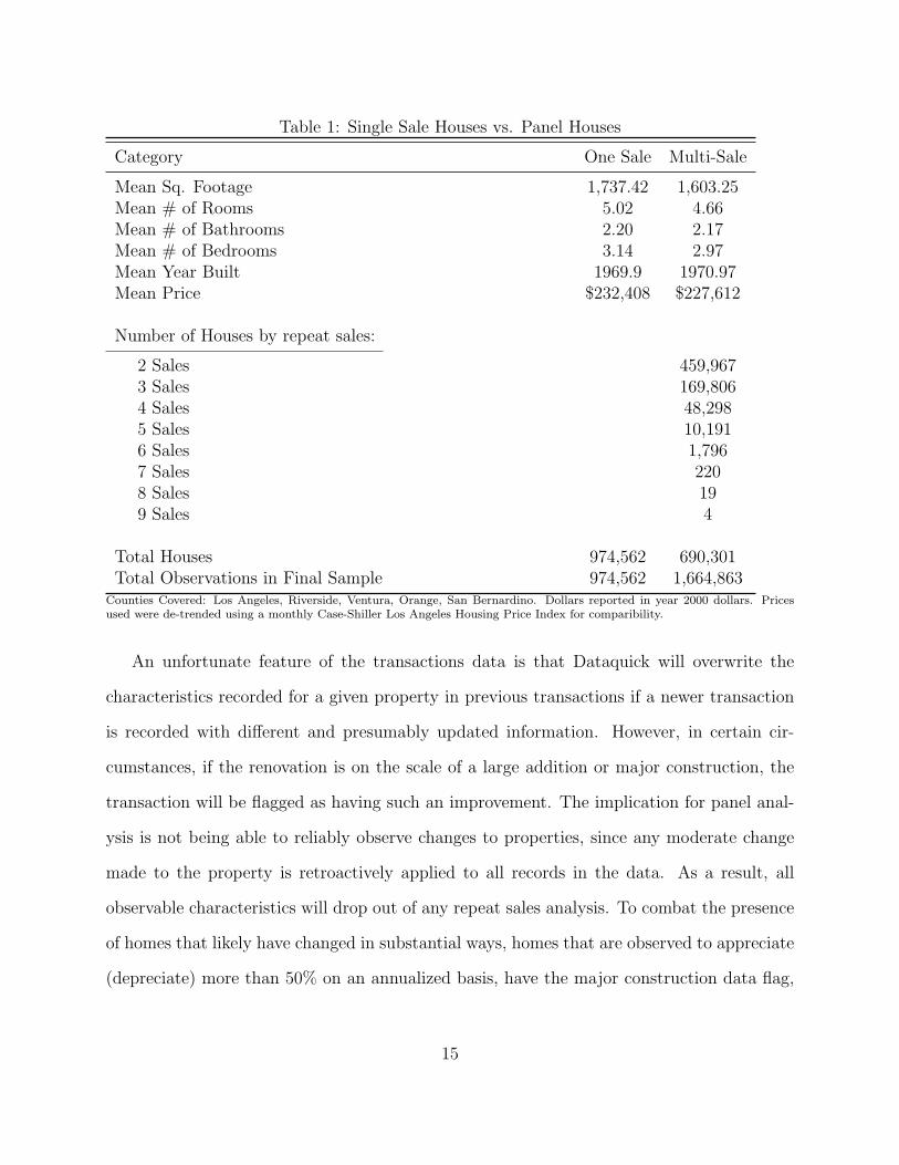
Table 1: Single Sale Houses vs. Panel Houses

Category One Sale Multi-Sale

Mean Sq. Footage 1,737.42 1,603.25Mean # of Rooms 5.02 4.66Mean # of Bathrooms 2.20 2.17Mean # of Bedrooms 3.14 2.97Mean Year Built 1969.9 1970.97Mean Price $232,408 $227,612

Number of Houses by repeat sales:

2 Sales 459,9673 Sales 169,8064 Sales 48,2985 Sales 10,1916 Sales 1,7967 Sales 2208 Sales 199 Sales 4

Total Houses 974,562 690,301Total Observations in Final Sample 974,562 1,664,863

Counties Covered: Los Angeles, Riverside, Ventura, Orange, San Bernardino. Dollars reported in year 2000 dollars. Pricesused were de-trended using a monthly Case-Shiller Los Angeles Housing Price Index for comparibility.

An unfortunate feature of the transactions data is that Dataquick will overwrite the

characteristics recorded for a given property in previous transactions if a newer transaction

is recorded with different and presumably updated information. However, in certain cir-

cumstances, if the renovation is on the scale of a large addition or major construction, the

transaction will be flagged as having such an improvement. The implication for panel anal-

ysis is not being able to reliably observe changes to properties, since any moderate change

made to the property is retroactively applied to all records in the data. As a result, all

observable characteristics will drop out of any repeat sales analysis. To combat the presence

of homes that likely have changed in substantial ways, homes that are observed to appreciate

(depreciate) more than 50% on an annualized basis, have the major construction data flag,

15

transact with a loan amount greater than the transaction price by $5,000, or are observed

to transact twice or more in any 12 month span are dropped from the sample.

Concern still remains that properties with unobserved changes are resident in the dataset.

If changes in properties are not correlated in any way with Superfund site exposure, then

unobserved property improvements should not bias any results. However, in a repeat-sales

model, the price effects of proximity to Superfund sites are identified by changes in site sta-

tus. If, for example, there is a correlation between home improvement and Superfund site

remediation, the estimated price effects of hazardous waste cleanup will be biased upwards as

it will be impossible to distinguish between those paying for improved environmental quality

and those paying for improved housing.

As a first-order test, it is possible to check whether the properties that have been dropped

from the sample as properties with suspected improvements are more likely to be in close

proximity to Superfund sites than those that aren’t likely to have received an improvement.

To conduct the test, for each property I note which transaction(s) cause it to be removed

from the main sample. Any property that is improved is then treated as improved for any

subsequent transactions I observe. Since a repeat-sales model will be biased if homes are

receiving unobserved improvements as Superfund sites are being remediated, I want to test

the relationship between changes in housing quality and changes in Superfund site status.

Consider the following binary response model:

Pr(Yit = 1|Zit) = Φ(Zitβ) (1)

Yit = Yit − Yit−1

Zit = Zit − Zit−1

where Yit = 1 if house i is renovated by time t and Yit = 0 otherwise, Zi is a vector

of hazardous waste measures for house i and year dummies, and Φ is the standard normal

16

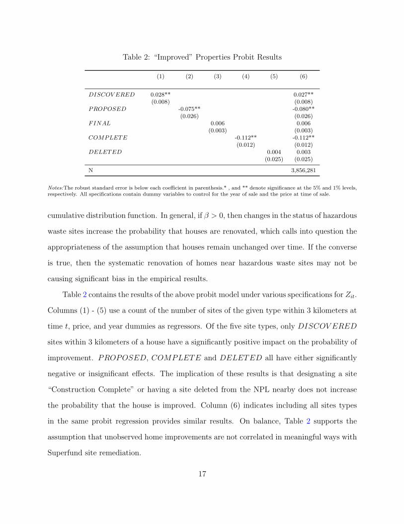
Table 2: “Improved” Properties Probit Results

(1) (2) (3) (4) (5) (6)

DISCOV ERED 0.028** 0.027**(0.008) (0.008)

PROPOSED -0.075** -0.080**(0.026) (0.026)

FINAL 0.006 0.006(0.003) (0.003)

COMPLETE -0.112** -0.112**(0.012) (0.012)

DELETED 0.004 0.003(0.025) (0.025)

N 3,856,281

Notes:The robust standard error is below each coefficient in parenthesis.* , and ** denote significance at the 5% and 1% levels,respectively. All specifications contain dummy variables to control for the year of sale and the price at time of sale.

cumulative distribution function. In general, if β > 0, then changes in the status of hazardous

waste sites increase the probability that houses are renovated, which calls into question the

appropriateness of the assumption that houses remain unchanged over time. If the converse

is true, then the systematic renovation of homes near hazardous waste sites may not be

causing significant bias in the empirical results.

Table 2 contains the results of the above probit model under various specifications for Zit.

Columns (1) - (5) use a count of the number of sites of the given type within 3 kilometers at

time t, price, and year dummies as regressors. Of the five site types, only DISCOV ERED

sites within 3 kilometers of a house have a significantly positive impact on the probability of

improvement. PROPOSED, COMPLETE and DELETED all have either significantly

negative or insignificant effects. The implication of these results is that designating a site

“Construction Complete” or having a site deleted from the NPL nearby does not increase

the probability that the house is improved. Column (6) indicates including all sites types

in the same probit regression provides similar results. On balance, Table 2 supports the

assumption that unobserved home improvements are not correlated in meaningful ways with

Superfund site remediation.

17

3.2 Superfund Site Data

The U.S. Environmental Protection Agency makes available via its website a comprehensive

data set detailing the names and locations of all hazardous waste sites reported to EPA and

the actions taken at these sites.7 Most important to this research, EPA details the date that

the site was discovered, the date any site was promoted to the Proposed National Priorities

list, the date any site moved from the Proposed NPL to the Final NPL, and the date any

site was deleted from the Final NPL. While not confidential, the dates that sites were listed

as “Construction Complete” and the verified location coordinates are not available in this

database and were provided directly by EPA. For this study, attention is restricted to the

set of hazardous waste sites that were proposed to be listed on the Final NPL (NPL sites)

by January 1, 2008. The principle reason for this restriction is that EPA has not verified the

longitude and latitude coordinates for non-NPL sites. As a result, I have a complete record

of action and location for 29 NPL sites within the five counties in the Los Angeles area; all

of which were at least proposed to the Final NPL in the timeframe in question.8

Table 3 provides a summary of how the Superfund site profile for the Greater Los Angeles

area has evolved over the sample period. At the end of 1990, there were no sites that were

being proposed to the Final NPL, listed as “Construction Complete”, or Deleted from the

NPL. By the end of 2000, there were still no Deleted NPL sites and only one site proposed

to the NPL. As would be expected, the majority of the remediation activities took place

later in the sample period. Census data would be unable to provide estimates of the price

effect of deleting a site from the NPL since there would be no variation in the data.

7The CERCLIS database can be downloaded in ASCII text format at http://www.epa.gov/superfund/sites/phonefax/products.htm

8One Superfund site was removed from the proposed NPL list and never listed. This site was droppedfrom the analysis since it is likely very different from the other sites that were all eventually listed.

18

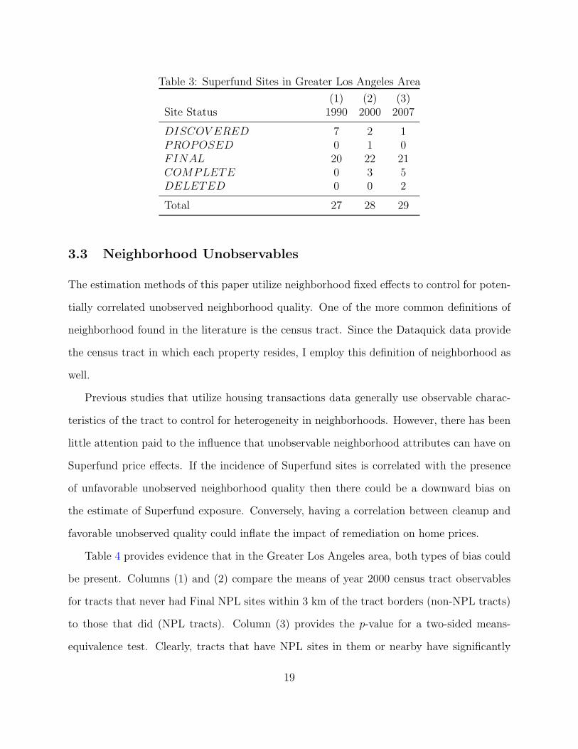
Table 3: Superfund Sites in Greater Los Angeles Area

(1) (2) (3)Site Status 1990 2000 2007

DISCOV ERED 7 2 1PROPOSED 0 1 0FINAL 20 22 21COMPLETE 0 3 5DELETED 0 0 2

Total 27 28 29

3.3 Neighborhood Unobservables

The estimation methods of this paper utilize neighborhood fixed effects to control for poten-

tially correlated unobserved neighborhood quality. One of the more common definitions of

neighborhood found in the literature is the census tract. Since the Dataquick data provide

the census tract in which each property resides, I employ this definition of neighborhood as

well.

Previous studies that utilize housing transactions data generally use observable charac-

teristics of the tract to control for heterogeneity in neighborhoods. However, there has been

little attention paid to the influence that unobservable neighborhood attributes can have on

Superfund price effects. If the incidence of Superfund sites is correlated with the presence

of unfavorable unobserved neighborhood quality then there could be a downward bias on

the estimate of Superfund exposure. Conversely, having a correlation between cleanup and

favorable unobserved quality could inflate the impact of remediation on home prices.

Table 4 provides evidence that in the Greater Los Angeles area, both types of bias could

be present. Columns (1) and (2) compare the means of year 2000 census tract observables

for tracts that never had Final NPL sites within 3 km of the tract borders (non-NPL tracts)

to those that did (NPL tracts). Column (3) provides the p-value for a two-sided means-

equivalence test. Clearly, tracts that have NPL sites in them or nearby have significantly

19

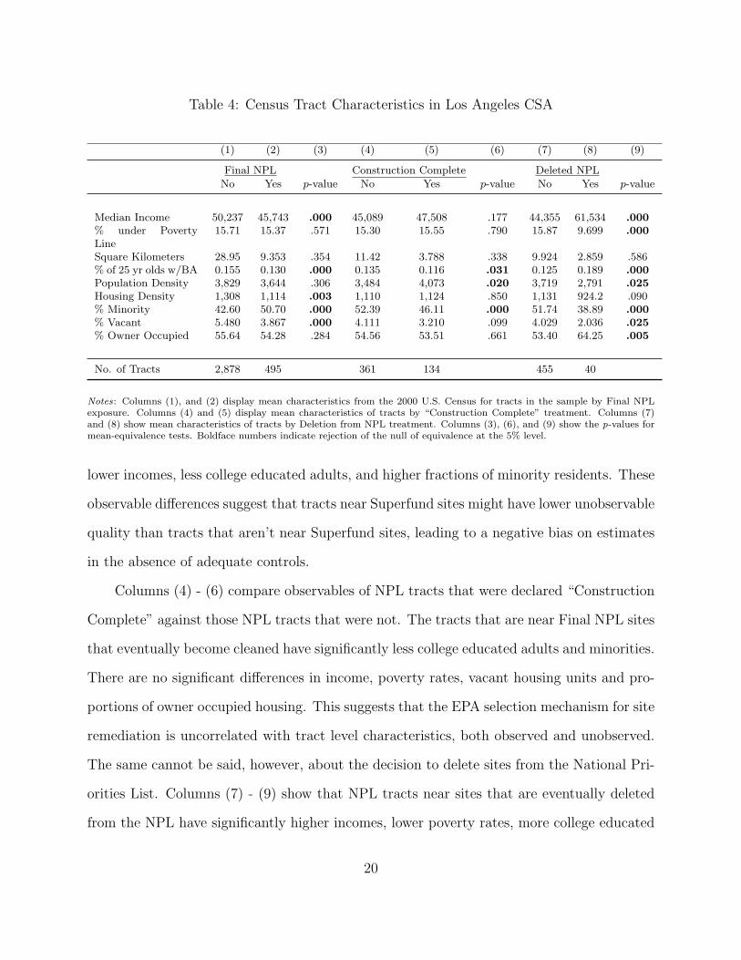
Table 4: Census Tract Characteristics in Los Angeles CSA

(1) (2) (3) (4) (5) (6) (7) (8) (9)

Final NPL Construction Complete Deleted NPL

No Yes p-value No Yes p-value No Yes p-value

Median Income 50,237 45,743 .000 45,089 47,508 .177 44,355 61,534 .000% under PovertyLine

15.71 15.37 .571 15.30 15.55 .790 15.87 9.699 .000

Square Kilometers 28.95 9.353 .354 11.42 3.788 .338 9.924 2.859 .586% of 25 yr olds w/BA 0.155 0.130 .000 0.135 0.116 .031 0.125 0.189 .000Population Density 3,829 3,644 .306 3,484 4,073 .020 3,719 2,791 .025Housing Density 1,308 1,114 .003 1,110 1,124 .850 1,131 924.2 .090% Minority 42.60 50.70 .000 52.39 46.11 .000 51.74 38.89 .000% Vacant 5.480 3.867 .000 4.111 3.210 .099 4.029 2.036 .025% Owner Occupied 55.64 54.28 .284 54.56 53.51 .661 53.40 64.25 .005

No. of Tracts 2,878 495 361 134 455 40

Notes: Columns (1), and (2) display mean characteristics from the 2000 U.S. Census for tracts in the sample by Final NPLexposure. Columns (4) and (5) display mean characteristics of tracts by “Construction Complete” treatment. Columns (7)and (8) show mean characteristics of tracts by Deletion from NPL treatment. Columns (3), (6), and (9) show the p-values formean-equivalence tests. Boldface numbers indicate rejection of the null of equivalence at the 5% level.

lower incomes, less college educated adults, and higher fractions of minority residents. These

observable differences suggest that tracts near Superfund sites might have lower unobservable

quality than tracts that aren’t near Superfund sites, leading to a negative bias on estimates

in the absence of adequate controls.

Columns (4) - (6) compare observables of NPL tracts that were declared “Construction

Complete” against those NPL tracts that were not. The tracts that are near Final NPL sites

that eventually become cleaned have significantly less college educated adults and minorities.

There are no significant differences in income, poverty rates, vacant housing units and pro-

portions of owner occupied housing. This suggests that the EPA selection mechanism for site

remediation is uncorrelated with tract level characteristics, both observed and unobserved.

The same cannot be said, however, about the decision to delete sites from the National Pri-

orities List. Columns (7) - (9) show that NPL tracts near sites that are eventually deleted

from the NPL have significantly higher incomes, lower poverty rates, more college educated

20

adults, less minorities, less vacant housing, higher proportions of owner occupied housing

and are less densely populated.9 It stands to reason that the sites that are deleted from the

NPL are in tracts with very positive unobservables and naıve estimates of the price effect of

deletion are likely to be positively biased.

3.4 House Level Unobservables

Controlling for unobserved heterogeneity at the neighborhood level may not be sufficient to

remove all omitted variable bias. When using tract-level fixed effects, identification comes

from within-tract variation. Given that the average size for tracts near NPL sites is approxi-

mately 9.4 square kilometers, the econometrician might be concerned that houses in the part

of a tract near a Superfund site could look very different in unobserved ways than houses in

another part of the tract. If houses near Superfund sites tend to be less well maintained and

updated than their counterparts within the tract, estimates without house-level controls for

endogeneity could be seriously biased.

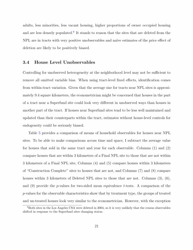
Table 5 provides a comparison of means of household observables for houses near NPL

sites. To be able to make comparisons across time and space, I subtract the average value

for houses that sold in the same tract and year for each observable. Columns (1) and (2)

compare houses that are within 3 kilometers of a Final NPL site to those that are not within

3 kilometers of a Final NPL site, Columns (4) and (5) compare houses within 3 kilometers

of “Construction Complete” sites to houses that are not, and Columns (7) and (8) compare

houses within 3 kilometers of Deleted NPL sites to those that are not. Columns (3), (6),

and (9) provide the p-values for two-sided mean equivalence t-tests. A comparison of the

p-values for the observable characteristics show that by treatment type, the groups of treated

and un-treated houses look very similar to the econometrician. However, with the exception

9Both sites in the Los Angeles CSA were deleted in 2004, so it is very unlikely that the census observablesshifted in response to the Superfund sites changing status.

21

Table 5: House Level Average Deviations from Tract-Level Means

(1) (2) (3) (4) (5) (6) (7) (8) (9)

Final NPL Construction Complete Deleted NPL

Yes No p-value Yes No p-value Yes No p-value

Price -880.5 53.51 .000 -514.5 2.334 .555 -4,589 4.720 .012No. of Bedrooms -0.00105 6.41e-05 .561 -0.00637 2.89e-05 .338 -0.0287 2.95e-05 .040No. of Bathrooms 0.00190 -0.000116 .200 -0.00259 1.18e-05 .633 -0.0187 1.93e-05 .101Square Footage 0.202 -0.0123 .870 -3.237 0.0147 .472 -16.94 0.0174 .073Year Built 0.0461 -0.00280 .130 0.187 -0.000849 .093 -0.202 0.000207 .389

Observations 152,435 2,508,130 12,016 2,648,549 2734 2,657,831

Notes: Columns (1), and (2) display the average demeaned characteristics for houses in the sample by Final NPL treatment.Columns (4) and (5) display the average demeaned characteristics for houses by “Construction Complete” treatment. Columns(7) and (8) display the average demeaned characteristics for houses by Deletion from NPL treatment. Treatment for a houseis defined as a house being within 3 kilometers of any site of the given type. Each variable for each house is demeaned bythe mean value observed for houses that sold in the same tract and year. Columns (3), (6), and (9) show the p-values formean-equivalence tests. Boldface numbers indicate rejection of the null of equivalence at the 5% level.

of the “Construction Complete” category, the respective groups have very different prices;

the houses near the sites have lower prices. While it may not be surprising that the only

difference between houses that are near sites and those that aren’t is that nearby houses

have lower prices, the data presented so far cannot distinguish between the case where lower

prices are caused by Superfund site proximity and the case where lower prices are caused by

lower unobserved housing quality near the sites. When the information contained in Table 5

is compared to the final results that control for unobserved heterogeneity, the argument for

the presence of lower unobserved quality becomes very strong.

4 Empirical Model

4.1 Hazardous Waste Measures

This paper departs from the prevalent measure for hazardous waste exposure, distance to

the nearest site, by counting the number of sites around each house. This method requires

22

selecting some maximum distance between a house and a site beyond which there is assumed

to be no price effect. As noted previously, some researchers have tried to estimate the distance

at which hazardous waste sites cease to affect home values with varying results. For this

study’s main specification, I count the number of sites that are within a 3 kilometer radius

of each house to measure the amount of hazardous waste exposure. However, the results are

robust to other specifications of distance.

Furthermore, to gain insight into how the life-cycle events of the Superfund program

separately influence the housing market, I include a measure of each of these steps. As

previously mentioned, in the context of my model, each hazardous waste site can be in

one of five stages at any given time: the DISCOV ERED period is the time after EPA is

aware of a potential hazard but before being proposed to the NPL; PROPOSAL is the time

after a site is proposed to the NPL but before a final listing on the NPL; FINAL is the

time after a site is listed on the Final NPL but before the site is designated “Construction

Complete”; COMPLETE is the time between designation as “Construction Completed”

and deletion from the NPL; DELETED is the time after EPA removes the site from the

NPL. These categories measure the major actions of the Superfund program that housing

market participants are likely to be interested in: the discovery of a hazardous waste site,

the potential for future cleanup, the promise of future cleanup, the completion of cleanup

and the verification of safety. Looking at the variation of housing prices as the density of

each type of Superfund site in close proximity varies can explain how each step is separately

valued in the market.

Since I know the location of each house and the location of each site, I can calculate the

distance between each pair. Furthermore, for each site, I know the timeframe for each of the

five periods above. Using transaction dates from the housing data, I can create a snapshot

of the hazardous waste profile around every house, specific to the day it was sold. The result

is a vector, for each house transaction, of counts of each of the five “types” of Superfund

23

sites nearby on the transaction date.

4.2 Main Specification

The general specification of this paper, given in Equation (2), assumes the hedonic price

function is linear in attributes. The price of any house i, sold at time t, in census tract j, is

a function of a vector of observable attributes of that house and a constant Xit, the vector of

hazardous waste site type counts in various stages, Zit, a fixed effect for which census tract

- year the house was sold in, δjt, an unobserved house attribute, γi, and an i.i.d. mean zero

disturbance term, εit. Data restrictions preclude me from observing changes in observable

characteristics Xit, therefore the subscript t is dropped.

lnPriceit = αXi + βZit + δjt + γi + εit (2)

Since Xi is constant over time, the coefficient α is unidentified. β is the coefficient of interest

and measures the effect that the density of hazardous waste sites in various stages in the

Superfund program have on the selling price of a home.

This specification explicitly accounts for both sources of bias discussed in Section 3. The

neighborhood level unobservable, δjt captures all determinants of price common to houses

that transact in a given tract and year. It’s worth noting that allowing the tract effect to

vary by year is a relaxation of the stronger assumption of time invariant neighborhood fixed

effects. Additionally, using observable characteristics from census years for data that is intra-

censal implicitly assumes that the tract is constant over time. This specification requires

no such assumption. House-level unobserved quality is controlled for by γi. Time-invariant

unobservables specific to each house that could bias estimates, such as aesthetics, hardwood

floors, gardens, abundant sunlight, historical significance, etc., will all be contained in this

term.

24

4.3 Flexible Distance Specification

The main specification assumes that the effect on price is constant inside a certain radius.

This restriction can be relaxed by splitting the radius of impact into expanding concentric

circles. For example, the main specification can be modified to count the number of sites

of each type separately that are present 0 - 1 km, 1 - 2 km, and 2 - 3 km from each house.

Under this alternate specification, Zit from Equation (2) expands in dimension to have three

sets of counts for each site status. Unobserved heterogeneity is controlled for in an identical

manner, and the model allows for distance from the site to have heterogenous impact.

4.4 Identification

Identification in the model described in Equation (2) requires successfully removing both δjt

and γi, the time-varying neighborhood fixed effect and the time-invariant house level fixed

effect, respectively. Careful attention must be paid to the method employed to remove these

unobservables. On the surface, Equation (2) is nothing more than a repeat-sales model

with a neighborhood fixed effect that changes overtime. However, since the data are an

unbalanced panel, using pre-packaged fixed effects routines or least-squares dummy variable

methods will be inconsistent.

To see why this is the case, consider for simplicity that each house sells only twice. First

differencing Equation (2) yields:

lnPriceit − lnPriceit−1 = α(Xi −Xi) + β(Zit − Zit−1) + (δjt − δjt−1) + (γi − γi) + (εit − εit−1)

(3)

¯lnPriceit = βZit + (δjt − δjt−1) + εit (4)

25

After first differencing, Equation (4) still has two unobserved terms: The neighborhood effect

in time t and the neighborhood effect in time t− 1. To mean difference away δjt, I need to

take the average of all first-differenced variables over the set of observations that had a sale

in neighborhood j and in time t. The problem arises from the fact that each observation

in this set has a second neighborhood unobservable that is not necessarily the same time as

δjt−1. Mean differencing removes δjt from Equation (4), but still leaves δjt−1 and the average

second neighborhood effect for all houses that sold in t. Using dummy variables for the

neighborhood-year fixed effects in Equation (4) and running OLS will leave this unobserved

“remainder” term and provide inconsistent estimates. To successfully remove both δjt and

δjt−1 from Equation (4), I must mean-difference by taking the average over the houses in

neighborhood j that sold in both years t and t− 1. This removes all unobserved terms and

provides a consistent estimate of β. Identification is driven by within-tract variation Super-

fund site exposure. Since the hazardous waste sites are always in existence and the distance

between sites and houses aren’t changing, identification comes from site status changes.

The identification strategy outlined above is built on several assumptions. First, β is not

indexed by either time or space, which implies that preferences over Superfund site exposure

remain constant throughout the entire sample period and the entire Los Angeles area. Sec-

ond, the house-level effect γi is assumed to be constant over time and data limitations force

the assumption of fixed housing observables. Third, counting the sites in a circle around

each house assumes the effect is constant within the radius of the circle.

Spatial variance in preferences is documented in the literature by site-specific studies.

The variance in estimates across the country and even within cities demonstrates both a

heterogeneity in Superfund sites and in preferences in local housing markets. While there

is no doubt a spatial distribution of preferences in Los Angeles10, this issue is intentionally

10See Redfearn (2009) for a discussion of spatial variation of preferences in hedonic studies and an appli-cation to light rail access in the Los Angeles area.

26

abstracted from in order to obtain an average estimate for the region. The robustness of

the assumption of time-invariant preferences is examined in the next section by allowing β

to vary by time periods. Section 3 examined the assumption of constant house level observ-

ables and unobservables. The evidence from the data suggests that improvements in housing

quality are not positively correlated with site status changes. Lastly, the robustness of the

assumption of constant impact within a 3 kilometer radius is examined by use of the flexible

distance specification and by examining results under various sizes of radii.

Finally, the research design raises concerns of correlated error terms. First, to control for

correlation in the error terms for each property i, standard errors are clustered on properties.

Second, there is concern that error terms in Equation (2) can be spatially autocorrelated. To

test for spatial autocorrelation, I group houses by their census tract and calculate Moran’s

I (MI) test statistic developed in Moran (1950) under various weighting schemes.11 For all

choices of weights, MI returned values very close to zero, indicating that the residuals are

not substantially spatially autocorrelated.

5 Results

5.1 Main Results

5.1.1 Site Count Specification

The results for the estimation of Equation (2) can be found in Column (1), Panel A of Table

6. Estimates of the various elements of β are listed with standard errors in parenthesis

underneath. EPA discovering an eventual NPL site actually raises home values by nearly

4%. Then, as the site is proposed, listed on the Final NPL and designated “Construction

Complete”, prices continue to rise. Panel B provides analysis of these step-by-step differences.

11See Case (1991) for a discussion of Moran’s I and testing for spatial autocorrelation in spatial demandmodels.

27

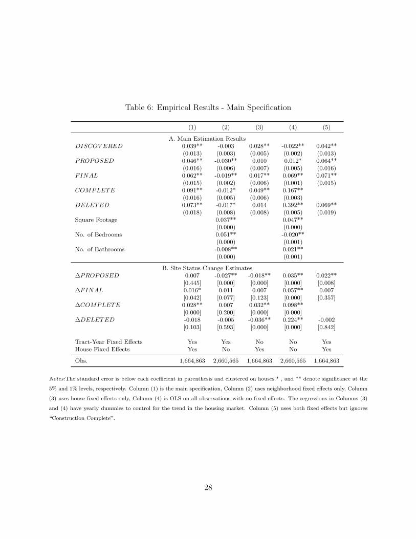
Table 6: Empirical Results - Main Specification

(1) (2) (3) (4) (5)

A. Main Estimation ResultsDISCOV ERED 0.039** -0.003 0.028** -0.022** 0.042**

(0.013) (0.003) (0.005) (0.002) (0.013)PROPOSED 0.046** -0.030** 0.010 0.012* 0.064**

(0.016) (0.006) (0.007) (0.005) (0.016)FINAL 0.062** -0.019** 0.017** 0.069** 0.071**

(0.015) (0.002) (0.006) (0.001) (0.015)COMPLETE 0.091** -0.012* 0.049** 0.167**

(0.016) (0.005) (0.006) (0.003)DELETED 0.073** -0.017* 0.014 0.392** 0.069**

(0.018) (0.008) (0.008) (0.005) (0.019)Square Footage 0.037** 0.047**

(0.000) (0.000)No. of Bedrooms 0.051** -0.020**

(0.000) (0.001)No. of Bathrooms -0.008** 0.021**

(0.000) (0.001)

B. Site Status Change Estimates∆PROPOSED 0.007 -0.027** -0.018** 0.035** 0.022**

[0.445] [0.000] [0.000] [0.000] [0.008]∆FINAL 0.016* 0.011 0.007 0.057** 0.007

[0.042] [0.077] [0.123] [0.000] [0.357]∆COMPLETE 0.028** 0.007 0.032** 0.098**

[0.000] [0.200] [0.000] [0.000]∆DELETED -0.018 -0.005 -0.036** 0.224** -0.002

[0.103] [0.593] [0.000] [0.000] [0.842]

Tract-Year Fixed Effects Yes Yes No No YesHouse Fixed Effects Yes No Yes No Yes

Obs. 1,664,863 2,660,565 1,664,863 2,660,565 1,664,863

Notes:The standard error is below each coefficient in parenthesis and clustered on houses.* , and ** denote significance at the

5% and 1% levels, respectively. Column (1) is the main specification, Column (2) uses neighborhood fixed effects only, Column

(3) uses house fixed effects only, Column (4) is OLS on all observations with no fixed effects. The regressions in Columns (3)

and (4) have yearly dummies to control for the trend in the housing market. Column (5) uses both fixed effects but ignores

“Construction Complete”.

28

Values in this panel represent the difference in the price effect that result from moving

from one site status to the next. Below each value in brackets is the p-value from a Wald

equivalence test. These tests reveal that proposing a site to the NPL and deleting a site from

the NPL do not have a statistically significant effect on prices, whereas listing a previously

proposed site on the Final NPL has a significantly positive effect of 1.6% and designating a

Final NPL site as “Construction Complete” has a significantly positive effect of 2.8%.

Columns (2) - (4) present estimates using different combinations of fixed effects: Column

(2) presents results without house level fixed effects and all single sale houses are included,

Column (3) presents results without tract-year fixed effects but with year dummies to control

for temporal market effects, and Column (4) presents the results with no fixed effects at all.

The estimates of the life-cycle changes in site status are all insignificant when not controlling

for fixed effects except for PROPOSED, which is negative. Ignoring the negative impact

that unobserved housing quality has on prices obscures the positive effects of the Superfund

program. Column (3) reveals that the absence of house-level fixed effects induces more bias

than the absence of tract-level fixed effects as the estimates are somewhat similar to the

main specification. However, Column (4) demonstrates the general influence of unobserved

heterogeneity. Without controlling for the unobserved quality of houses and neighborhoods

in close proximity of Superfund sites, the estimated benefit of designating a Final NPL site

as “Construction Complete” is 9.8% and the benefit of taking a “Construction Complete”

site off of the NPL is an additional 22.4%. Finally, Column (5) provides results from a model

that uses the same fixed effects as Column (1) but ignores “Construction Complete” as a

site status. Under this specification, all price improvements are realized at site discovery

and proposal to the NPL. This finding is consistent with previous studies that ignored

“Construction Complete” and found no effect for final listing on the NPL and deletion from

the NPL.

One counterintuitive result is the large, positive coefficient on DISCOV ERED. It

29

might be expected that discovering a nearby site is posing health risks would negatively

impact prices. One possibility is that rising housing prices cause discovery. If prices are

rising exogenously by an influx of new buyers, then hazardous waste spills have a higher

probability of being discovered. This can lead to a situation where sites are being discovered

only after additional residents enter the area and drive up prices. Furthermore, the probit

model from Section 3 indicated that site discovery increases the probability of houses being

renovated. Discovery of sites could be endogenous with reinvestment in the community. This

phenomenon should be addressed by future research.

5.1.2 Flexible Distance Specification

Table 7 provides estimates of the flexible distance estimator. In Panel A, Columns (1) - (3)

list the coefficients of the regression corresponding to the main specification where the counts

of each site type are broken out by whether they fall within 0 - 1 kilometers, 1 - 2 kilometers,

or 2 - 3 kilometers. They are presented horizontally for ease of comparison. Moving down

each column documents how, for a given distance band, the estimated coefficient changes as

site status changes. Panel B provides these differences by distance bands along with p-values

from Wald tests of equivalence. Moving across any row in Panel A allows comparison of the

effect a site of that type has on prices as distance increases. Panel C lists the difference in

coefficients with p-values from Wald tests of equivalence underneath in brackets. Finally,

Panel D reports the difference in site status change effects and tests for equivalence between

distance bands.

Several important facts emerge from Table 7 Panel B. First, the effect of deleting a

site has a negative and significant effect at 0 - 1 km and 1 - 2 km, whereas the main

specification reports no significant effect for deletion. Second, the effect of designating a site

“Construction Complete” has positive, significant effects on price that are stronger at closer

distances. Panel D reveals that this effect is significantly lower at the farthest distance band.

30

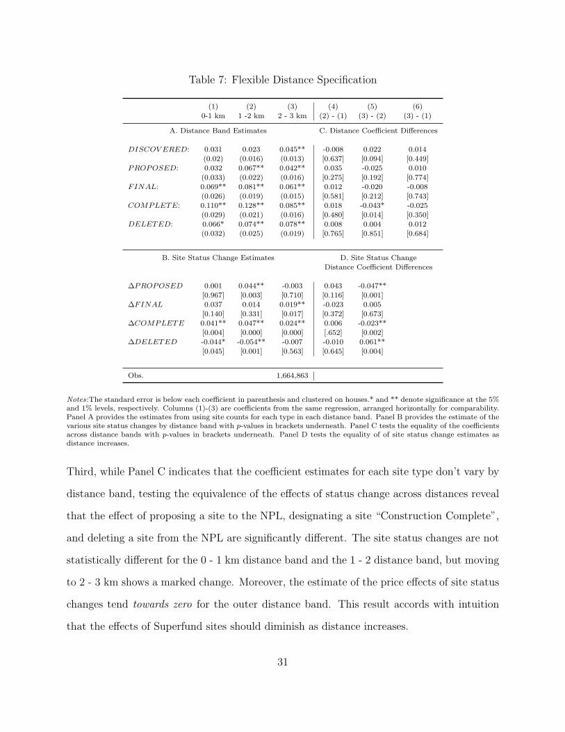
Table 7: Flexible Distance Specification

(1) (2) (3) (4) (5) (6)

0-1 km 1 -2 km 2 - 3 km (2) - (1) (3) - (2) (3) - (1)

A. Distance Band Estimates C. Distance Coefficient Differences

DISCOV ERED: 0.031 0.023 0.045** -0.008 0.022 0.014

(0.02) (0.016) (0.013) [0.637] [0.094] [0.449]

PROPOSED: 0.032 0.067** 0.042** 0.035 -0.025 0.010

(0.033) (0.022) (0.016) [0.275] [0.192] [0.774]

FINAL: 0.069** 0.081** 0.061** 0.012 -0.020 -0.008

(0.026) (0.019) (0.015) [0.581] [0.212] [0.743]

COMPLETE: 0.110** 0.128** 0.085** 0.018 -0.043* -0.025

(0.029) (0.021) (0.016) [0.480] [0.014] [0.350]

DELETED: 0.066* 0.074** 0.078** 0.008 0.004 0.012

(0.032) (0.025) (0.019) [0.765] [0.851] [0.684]

B. Site Status Change Estimates D. Site Status Change

Distance Coefficient Differences

∆PROPOSED 0.001 0.044** -0.003 0.043 -0.047**

[0.967] [0.003] [0.710] [0.116] [0.001]

∆FINAL 0.037 0.014 0.019** -0.023 0.005

[0.140] [0.331] [0.017] [0.372] [0.673]

∆COMPLETE 0.041** 0.047** 0.024** 0.006 -0.023**

[0.004] [0.000] [0.000] [.652] [0.002]

∆DELETED -0.044* -0.054** -0.007 -0.010 0.061**

[0.045] [0.001] [0.563] [0.645] [0.004]

Obs. 1,664,863

Notes:The standard error is below each coefficient in parenthesis and clustered on houses.* and ** denote significance at the 5%and 1% levels, respectively. Columns (1)-(3) are coefficients from the same regression, arranged horizontally for comparability.Panel A provides the estimates from using site counts for each type in each distance band. Panel B provides the estimate of thevarious site status changes by distance band with p-values in brackets underneath. Panel C tests the equality of the coefficientsacross distance bands with p-values in brackets underneath. Panel D tests the equality of of site status change estimates asdistance increases.

Third, while Panel C indicates that the coefficient estimates for each site type don’t vary by

distance band, testing the equivalence of the effects of status change across distances reveal

that the effect of proposing a site to the NPL, designating a site “Construction Complete”,

and deleting a site from the NPL are significantly different. The site status changes are not

statistically different for the 0 - 1 km distance band and the 1 - 2 distance band, but moving

to 2 - 3 km shows a marked change. Moreover, the estimate of the price effects of site status

changes tend towards zero for the outer distance band. This result accords with intuition

that the effects of Superfund sites should diminish as distance increases.

31

5.2 Robustness

In this subsection I provide results demonstrating the robustness of the results presented

so far. First, I examine the assumption of a time-constant hedonic price surface and find

that the preferences that give rise to the implicit prices appear to be relatively constant over

time. Second, I vary the size of the exposure circles used in the main specification and show

similar conclusions can be drawn about the Superfund program’s effects.

5.2.1 Time Varying Preferences

The identification strategy assumes that β is the same in all periods. This can be a troubling

assumption given the twenty year sample period. Its very plausible that the hedonic price

surface shifts throughout the time period. To check the sensitivity of the results to this

assumption, I estimate a similar model to the main specification that allows preferences to

change over time. I break the sample period into four 5-year periods and estimate separate

coefficients for each.

Consider rewriting Equation (2) the following way:

lnPriceit = αXi + β1Zit ∗ I{t ∈ E1}+ β2Zit ∗ I{t ∈ E2}+

β3Zit ∗ I{t ∈ E3}+ β4Zit ∗ I{t ∈ E4}+ δjt + γi + εit (5)

where I{·} is the indicator function, {E1, E2, E3, E4} correspond to the first, second, third

and fourth 5-year era in the dataset, {β1, β2, β3, β4} are the time varying parameters, and

Xi, α, and Zit have the same interpretation as in the main specification. If these parame-

ters are not statistically different from each other, then identification concerns of the main

specification should be mitigated. Note that this example differences away the unobserved

error terms the in the same way as the main specification.

Table 8 provides the coefficient estimates for Equation (5). Columns (5) - (7) provide

32

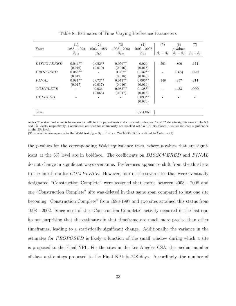
Table 8: Estimates of Time Varying Preference Parameters

(1) (2) (3) (4) (5) (6) (7)Years 1988 - 1992 1993 - 1997 1998 - 2002 2003 - 2008 p-values

β1,k β2,k β3,k β4,k β2 − β1 β3 − β2 β4 − β3

DISCOV ERED 0.044** 0.052** 0.056** 0.029 .501 .800 .174(0.016) (0.019) (0.016) (0.018)

PROPOSED 0.066** - 0.037* 0.132** - .046† .020(0.019) (0.018) (0.040)

FINAL 0.081** 0.072** 0.071** 0.066** .146 .957 .214(0.017) (0.017) (0.016) (0.016)

COMPLETE - 0.034 0.083** 0.128** - .433 .000(0.065) (0.017) (0.018)

DELETED - - - 0.090** - - -(0.020)

Obs. 1,664,863

Notes:The standard error is below each coefficient in parenthesis and clustered on houses.* and ** denote significance at the 5%and 1% levels, respectively. Coefficients omitted for collinearity are marked with a ”-”. Boldfaced p-values indicate significanceat the 5% level.†This p-value corresponds to the Wald test β3 − β1 = 0 since PROPOSED is omitted in Column (2).

the p-values for the corresponding Wald equivalence tests, where p-values that are signif-

icant at the 5% level are in boldface. The coefficients on DISCOV ERED and FINAL

do not change in significant ways over time. Preferences appear to shift from the third era

to the fourth era for COMPLETE. However, four of the seven sites that were eventually

designated “Construction Complete” were assigned that status between 2003 - 2008 and

one “Construction Complete” site was deleted in that same span compared to just one site

becoming “Construction Complete” from 1993-1997 and two sites attained this status from

1998 - 2002. Since most of the “Construction Complete” activity occurred in the last era,

its not surprising that the estimates in that timeframe are much more precise than other

timeframes, leading to a statistically significant change. Additionally, the variance in the

estimates for PROPOSED is likely a function of the small window during which a site

is proposed to the Final NPL. For the sites in the Los Angeles CSA, the median number

of days a site stays proposed to the Final NPL is 248 days. Accordingly, the number of

33

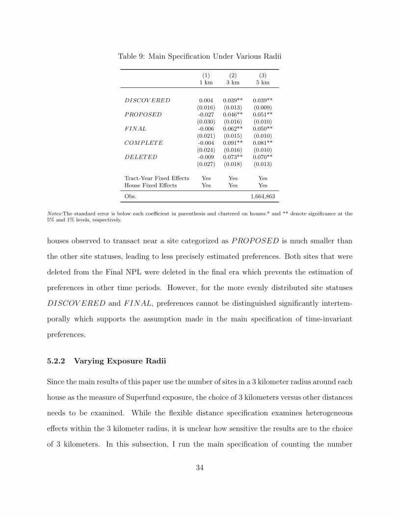
Table 9: Main Specification Under Various Radii

(1) (2) (3)1 km 3 km 5 km

DISCOV ERED 0.004 0.039** 0.039**(0.016) (0.013) (0.009)

PROPOSED -0.027 0.046** 0.051**(0.030) (0.016) (0.010)

FINAL -0.006 0.062** 0.050**(0.021) (0.015) (0.010)

COMPLETE -0.004 0.091** 0.081**(0.024) (0.016) (0.010)

DELETED -0.009 0.073** 0.070**(0.027) (0.018) (0.013)

Tract-Year Fixed Effects Yes Yes YesHouse Fixed Effects Yes Yes Yes

Obs. 1,664,863

Notes:The standard error is below each coefficient in parenthesis and clustered on houses.* and ** denote significance at the5% and 1% levels, respectively.

houses observed to transact near a site categorized as PROPOSED is much smaller than

the other site statuses, leading to less precisely estimated preferences. Both sites that were

deleted from the Final NPL were deleted in the final era which prevents the estimation of

preferences in other time periods. However, for the more evenly distributed site statuses

DISCOV ERED and FINAL, preferences cannot be distinguished significantly intertem-

porally which supports the assumption made in the main specification of time-invariant

preferences.

5.2.2 Varying Exposure Radii

Since the main results of this paper use the number of sites in a 3 kilometer radius around each

house as the measure of Superfund exposure, the choice of 3 kilometers versus other distances

needs to be examined. While the flexible distance specification examines heterogeneous

effects within the 3 kilometer radius, it is unclear how sensitive the results are to the choice

of 3 kilometers. In this subsection, I run the main specification of counting the number

34

of sites of each type in a radius around each house at 2 different radii: 1 kilometer and 5

kilometers. Kiel and Zabel (2001) estimate the maximum distance for price effects to be

three miles, or 4.828 kilometers, so I use 5 kilometers as a comparison on the larger side.

Conversely, it is interesting to see how the estimates change when restricting the exposure

window to only 1 kilometer.

Table 9 contains the results of the regression defined in Equation (2) under 1, 3, and 5 km

radii, respectively. A comparison of Columns (2) and (3) reveals that changing the radius

from 3 km to 5 km has little impact on the sign, significance and magnitude of the coefficients.

However, when restricting the radius to 1 km the estimates all become insignificant. While

intuition would suggest that the impact of Superfund sites on the housing market should be

larger closer to the sites, these results suggest that homeowners that sort themselves in close

proximity to Superfund sites don’t care about hazardous waste exposure. Individuals who

are responsive to the risks of living near Superfund sites don’t live in close proximity, so as

sites are remediated, homeowners that are sensitive to environmental quality capitalize the

improvement at the farther distances.

5.3 Nearest-Site Results

The prevailing method for capturing exposure to Superfund sites is to use the distance to

the nearest site as the measure of disamenity. If Superfund sites are clustered and many

houses are in close proximity to multiple sites, nearest-site methods can suffer from an

omitted variables problem that the site-counting method will not. Conversely, if clustering

of Superfund sites is not prevalent, then the site-counting method is similar to using distance

to the nearest site. In the limit, if no house has more than one house nearby, then the site-

count method reduces to the nearest-site method with the exposure measure becoming a

simple function of distance equal to 1 if a site is within a certain radius, and 0 otherwise.

To compare the results using the site-count method to the traditional distance to nearest

35

site method, I employ a proximity function similar to that found in Kiel and Zabel (2001):

PROXi = max(0, D0 −Di) (6)

where Di is the distance from house i to the nearest site and D0 represents the maximum

distance of Superfund site influence, which is set to 5 km.12 To make a fair comparison, I

maintain the use of both sets of fixed effects. Consider the following regression equation:

lnPriceit = αXi + β′Zit ∗ PROXi + δjt + γi + εit (7)

where β is a (5×1) vector of parameters, Zit is a (5×1) vector of dummy variables indicating

the status of the nearest site to house i at the time of sale, PROXi is the proximity function

in Equation (6), and δjt and γi are the tract-year and house-level fixed effects, respectively.

Column (1) of Table 10 provides the results of estimating Equation (7) while Column

(2) provides the differences in coefficients and the associated p-value from the Wald test of

equivalence. The coefficients are most easily interpreted as the marginal value for a house

with PROXi = 1, or a house that is 4 km away from a Superfund site. These estimates

are somewhat similar to those found in the main results. Specifically, the largest and most

significant improvement in price, 2.3%, comes when a site is designated “Construction Com-

plete”. These results show an improvement in price when a site is proposed to the Final

NPL whereas the previous results measured the improvement at final listing on the NPL.

Both sets of results indicate no significant change in price when a site is deleted from the

NPL.

Column (3) provides estimation results when additional regressors measuring the prox-

imity to the second nearest site are included. The goal of this regression is to capture the

extent to which multiple sites can contribute to an omitted variables problem. In the Los

12As mentioned in the previous section, Kiel and Zabel (2001) find D0 = 3 miles, which is roughly 5 km.

36

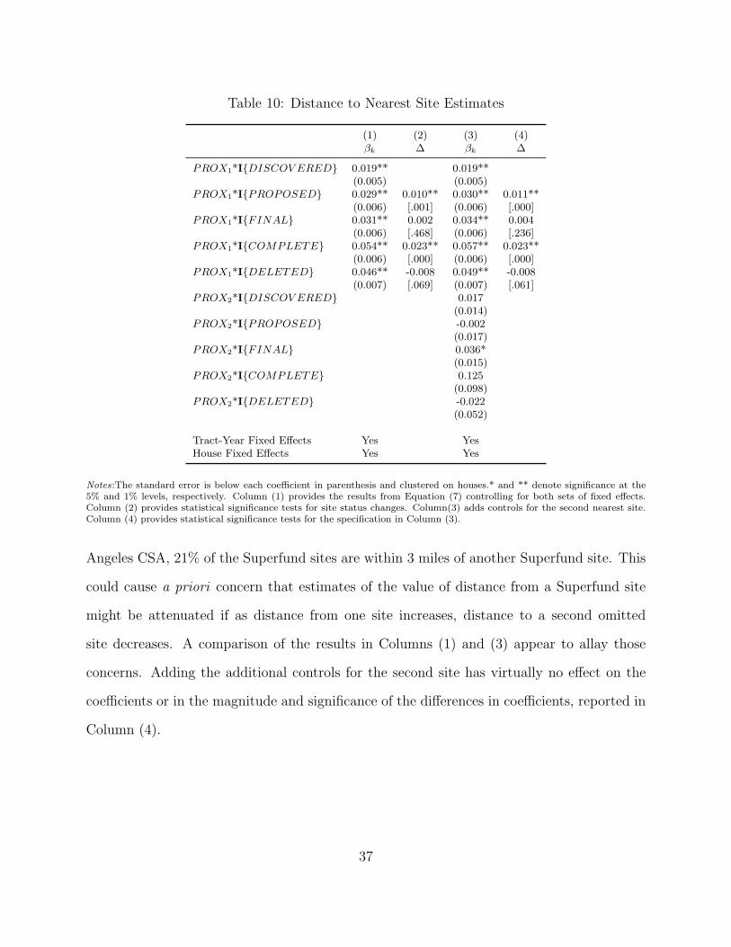
Table 10: Distance to Nearest Site Estimates

(1) (2) (3) (4)βk ∆ βk ∆

PROX1*I{DISCOV ERED} 0.019** 0.019**(0.005) (0.005)

PROX1*I{PROPOSED} 0.029** 0.010** 0.030** 0.011**(0.006) [.001] (0.006) [.000]

PROX1*I{FINAL} 0.031** 0.002 0.034** 0.004(0.006) [.468] (0.006) [.236]

PROX1*I{COMPLETE} 0.054** 0.023** 0.057** 0.023**(0.006) [.000] (0.006) [.000]

PROX1*I{DELETED} 0.046** -0.008 0.049** -0.008(0.007) [.069] (0.007) [.061]

PROX2*I{DISCOV ERED} 0.017(0.014)

PROX2*I{PROPOSED} -0.002(0.017)

PROX2*I{FINAL} 0.036*(0.015)

PROX2*I{COMPLETE} 0.125(0.098)

PROX2*I{DELETED} -0.022(0.052)

Tract-Year Fixed Effects Yes YesHouse Fixed Effects Yes Yes

Notes:The standard error is below each coefficient in parenthesis and clustered on houses.* and ** denote significance at the5% and 1% levels, respectively. Column (1) provides the results from Equation (7) controlling for both sets of fixed effects.Column (2) provides statistical significance tests for site status changes. Column(3) adds controls for the second nearest site.Column (4) provides statistical significance tests for the specification in Column (3).

Angeles CSA, 21% of the Superfund sites are within 3 miles of another Superfund site. This

could cause a priori concern that estimates of the value of distance from a Superfund site

might be attenuated if as distance from one site increases, distance to a second omitted

site decreases. A comparison of the results in Columns (1) and (3) appear to allay those

concerns. Adding the additional controls for the second site has virtually no effect on the

coefficients or in the magnitude and significance of the differences in coefficients, reported in

Column (4).

37

5.4 Discussion

One of the main goals of this study is to separately value the life-cycle effects of Superfund

sites in a region. The positive impact on prices of designating a site as “Construction Com-

plete” is the most robust finding. The effects are seen at small and large radii, are positive

over time, and are invariant to the use of site-counts or distance to the nearest site. This

result comes in contrast to those studies in the literature that focus solely on deletion from

the NPL as the indicator of site remediation. My results suggest information about the

remediation of Superfund sites is communicated well before deletion from the NPL takes

place, causing the effect of deletion to be insignificant. Additionally, my main results show

that there is a significant increase in prices once a site is actually listed on the Final NPL,

suggesting that the promise of future remediation registers positively on prices.

Second, the importance of controlling for unobserved heterogeneity cannot be under-

stated. While the importance of house-level fixed effects appear to be relatively greater, not

controlling for both house-level and neighborhood-level unobserved quality will lead to bi-

ased estimates. Many of the existing site-specific studies ignore unobserved housing quality

and control for neighborhood quality by using the most recent census data, which might

not be constant throughout the sample period. Using tract-year fixed effects eliminates this

problem, while effectively controlling for these unobserved elements.

Third, while the results of this study are only applicable to the Greater Los Angeles

area, they are generalizable to any site in the region and the methods are generalizable to

any metropolitan area where housing transactions data are available. A balance is struck

between national studies, which impose homogeneity on Superfund sites and preferences,

and site-specific studies, which allow for heterogeneous sites but are not generalizable. The

result is a method that measures the idiosyncratic preferences of a region while averaging

over a small sample of sites, allowing estimates to be applied to new sites outside of the

38

current study.13

Finally, the importance of omitted variable bias in studies that utilize distance to the

nearest Superfund site as the measure of exposure is examined and found to be minimal in

the Los Angeles area. The results show that adding the distance to the second nearest site

has little impact on the estimates for proximity. In this case, the results mimic those of the

site-count method introduced in this paper. However, the mitigation of the omitted variable

bias is likely do more to the use of house-level fixed effects than to the general robustness

of nearest-site methods. In a repeat sales model, distance to the second site is differenced

away, unless the site changes status between sales. For any given supply of houses in close

proximity to multiple sites, the subset of observations where the “second site” changes status

simultaneously with the “first site” will be smaller, reducing the impact that the “second

site” has on repeat sales estimates. Since the site-count method doesn’t ignore the presence

of multiple sites and provides similar results to existing methods in the absence of omit-

ted variables bias, it is demonstrated to be a valuable addition to the literature on valuing

environmental disamenities.

6 Conclusion

This paper argues policy relevant estimates of the price effects in the housing market of

Superfund site remediation requires a regional or city level analysis. If policymakers require

an estimate of the value of remediating a particular site, national sample estimates derived

from the average preferences of U.S. homeowners, not of the local homeowners who will

be affected by action, may be insufficient. Conversely, estimates derived from site-specific

analyses might not be externally applicable if the analysis was in a different region or a

13Applying the estimates to sites within the study is also a benefit of this study. For instance, policymakershave an estimate of the value of taking a particular site that is currently on the Final NPL to “ConstructionComplete” status.

39

different site, since estimates will be a function of a particular site’s idiosyncrasies. Averaging

over multiple sites and measuring the preferences of a particular region provides estimates

that are applicable to other sites in the region of interest. This paper demonstrates a

method for obtaining consistent estimates of the various life-cycle events of Superfund site

remediation that is generalizable to any area where housing transactions data are available.

The results suggest that different actions undertaken by EPA communicate different

things to the housing market. Listing a site on the Final NPL is shown to increase nearby

housing prices by 1.6%. This suggests that at the time of listing, the externality of hazardous

waste proximity was already capitalized and the promise of remediation is enough to move

prices upward. Once EPA designates a site as “Construction Complete”, local housing

prices gain an additional 2.8%. Deletion of an NPL site seems to have no significant impact

on prices. While the absence of an effect for deleting a site from the NPL is in line with

estimates from previous research, the results for the impact of listing a site on the Final NPL

and designating a site as “Construction Complete” demonstrate a break from the literature

that attempts to estimate average effects across multiple sites.

The lack of evidence of a positive price impact of Superfund site remediation from hedonic

pricing studies has called into question the return on investment for the high cost of site

remediation. This paper demonstrates a clear, positive impact on prices as a result of the

Superfund program, the largest of which comes directly from the act of cleaning a site, not

deleting it from the NPL. While this result comes with the caveat of being applicable only

to the Los Angeles CSA, the point is made that one-size-fits-all national estimates obscure

the heterogeneity in regional preferences. There is no doubt that there are certain areas of

the country which are likely to place low value on site remediation and some areas which

will place a high value on site remediation. Any remediation decision should be made in

reference to the preferences of the local populace, not the average preferences of the nation

or the idiosyncratic preferences of homeowners around one particular site remediated in the

40

past. This study establishes the influence of this distinction in approach on conclusions

drawn about the benefits to the housing market of the Superfund program.

41

References

Bartik, T. J. (1987a). Estimating Hedonic Demand Parameters with Single Market Data:The Problems Caused by Unobserved Tastes. Review of Economics and Statistics,69(1):178–180.

Bartik, T. J. (1987b). The Estimation of Demand Parameters in Hedonic Price Models.Journal of Political Economy, 95(1):81–88.

Brown, J. N. and Rosen, H. S. (1982). On the Estimation of Structual Hedonic Price Models.Econometrica, 50(3):765–768.

Cameron, T. A. (2006). Directional heterogeneity in distance profiles in hedonic propertyvalue models. Journal of Environmental Economics and Management, 51:26 – 45.

Case, A. C. (Jul., 1991). Spatial patterns in household demand. Econometrica, 59(4):953–965.

Clinton, W. J. (1993). Executive Order 12886: Federal Regulation. Federal Register, 58(190).

Epple, D. (1987). Hedonic Prices and Implicit Markets: Estimating Demand and SupplyFunctions for Differentiated Products. Journal of Political Economy, 95(1):59–80.

Farber, S. (1998). Undesirable facilities and property values: a summary of empirical studies.Ecological Economics, 24:1–14.

Gayer, T., Hamilton, J. T., and Viscusi, W. K. (2000). Private values of risk tradeoffs atsuperfund sites: Housing market evidence on learning about risk. Review of Economicsand Statistics, 82(3):439–451.

Greenberg, M. and Hughes, J. (1992). The impact of hazardous waste Superfund sites onthe value of houses sold in New Jersey. The Annals of Regional Science, 26(2):147–153.

Greenstone, M. and Gallagher, J. (2008). Does hazardous waste matter? evidence from thehousing market and the superfund program. Quarterly Journal of Economics, 123(3):951–1003.

Gupta, S., Van Houtven, G., and Cropper, M. (1996). Paying for permanence: an economicanalysis of EPA’s cleanup decisions at Superfund sites. RAND Journal of Economics,27(3):563–582.

Hite, D., Chern, W., Hitzhusen, F., and Randall, A. (2001). Property-Value Impacts of anEnvironmental Disamenity: The Case of Landfills. Journal of Real Estate Finance andEconomics, 22(2/3):185–202.

Kiel, K. and Williams, M. (2007). The impact of Superfund sites on local property values:Are all sites the same? Journal of Urban Economics, 61:170–192.

42

Kiel, K. and Zabel, J. (2001). Estimating the Economics Benefits of Cleaning Up Super-fund Sites: The Case of Woburn, Massachusetts. Journal of Real Estate Finance andEconomics, 22(2/3):163–184.

Kohlhase, J. E. (1991). The impact of toxic waste sites on housing values. Journal of UrbanEconomics, 30:1–26.

Michaels, R. G. and Smith, V. K. (1990). Market segmentation and valuing amenities withhedonic models: The case of hazardous waste sites. Journal of Urban Economics, 28:223–242.

Moran, P. A. P. (1950). Notes on continuous stochastic phenomena. Biometrika, 37(1/2):17–23.

Noonan, D. S., Krupka, D. J., and Baden, B. M. (2007). Neighborhood Dynamics and PriceEffects of Superfund Site Clean-up. Journal of Regional Science, 47(4):665–692.

Palmquist, R. B. (1984). Estimating the Demand for the Characteristics of Housing. TheReview of Economics and Statistics, 66(3):394–404.

Reagan, R. (1981). Executive Order 12291: Federal Regulation. Federal Register, page 46FR 13193. Revoked by E.O. 12886.

Redfearn, C. L. (2009). How informative are average effects? Hedonic regression and amenitycapitalization in complex urban housing markets. Regional Science and Urban Economics,39(3):297 – 306.

Rosen, S. (1974). Hedonic prices and implicit markets: Product differentiation in purecompetition. Journal of Political Economy, 82(1):34–55.

43