Embed Size (px)
Citation preview
Hidden Process Modelswith Applications to fMRI Data
Rebecca A. HutchinsonMarch 24, 2010
Biostatistics and Biomathematics SeminarFred Hutchinson Cancer Research Center
2
Introduction
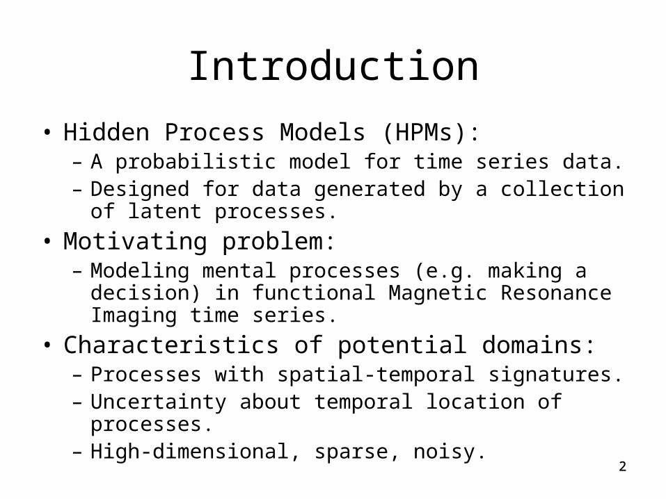
• Hidden Process Models (HPMs): – A probabilistic model for time series data.– Designed for data generated by a collection of latent
processes.
• Motivating problem:– Modeling mental processes (e.g. making a decision)
in functional Magnetic Resonance Imaging time series.
• Characteristics of potential domains:– Processes with spatial-temporal signatures.– Uncertainty about temporal location of processes.– High-dimensional, sparse, noisy.
2
3
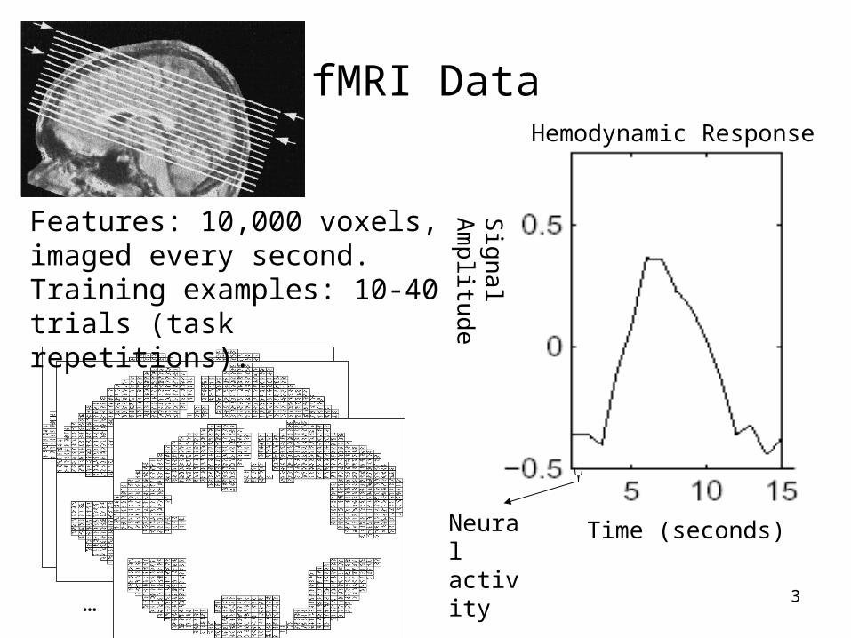
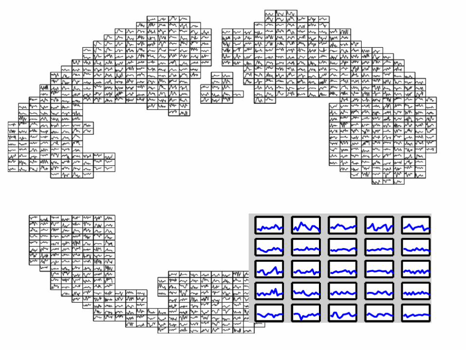
fMRI Data
…
Sign
al
Am
plitu
de
Time (seconds)
Hemodynamic Response
Neural activity
Features: 10,000 voxels, imaged every second.Training examples: 10-40 trials (task repetitions).
4
5
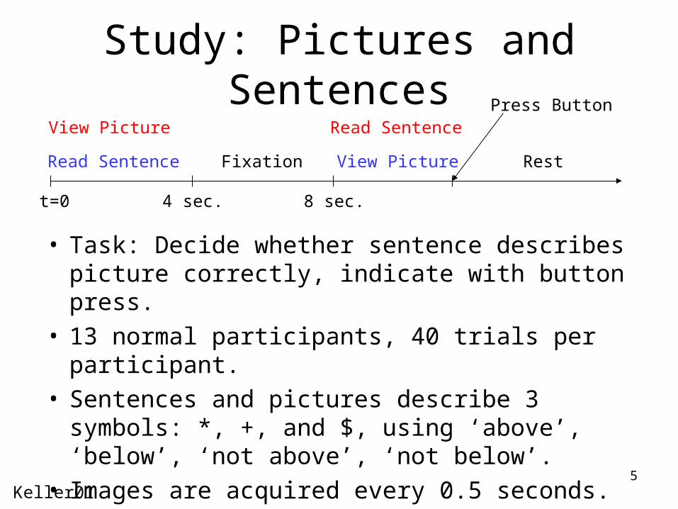
Study: Pictures and Sentences
• Task: Decide whether sentence describes picture correctly, indicate with button press.
• 13 normal participants, 40 trials per participant.• Sentences and pictures describe 3 symbols: *,
+, and $, using ‘above’, ‘below’, ‘not above’, ‘not below’.
• Images are acquired every 0.5 seconds.
Read Sentence
View Picture Read Sentence
View PictureFixation
Press Button
4 sec. 8 sec.t=0
Rest
Keller01
6
Motivation
• To track mental processes over time. – Estimate process hemodynamic responses.– Estimate process timings.
• Allowing processes that do not directly correspond to the stimuli timing is a key contribution of HPMs!
• To compare hypotheses of cognitive behavior.
7
Related Work
• fMRI– General Linear Model (Dale99)
• Must assume timing of process onset to estimate hemodynamic response.
– Computer models of human cognition (Just99, Anderson04)• Predict fMRI data rather than learning parameters of processes from
the data.
• Machine Learning – Classification of windows of fMRI data (overview in Haynes06)
• Does not typically model overlapping hemodynamic responses.
– Dynamic Bayes Networks (Murphy02, Ghahramani97)• HPM assumptions/constraints can be encoded by extending
factorial HMMs with links between the Markov chains.
7
8
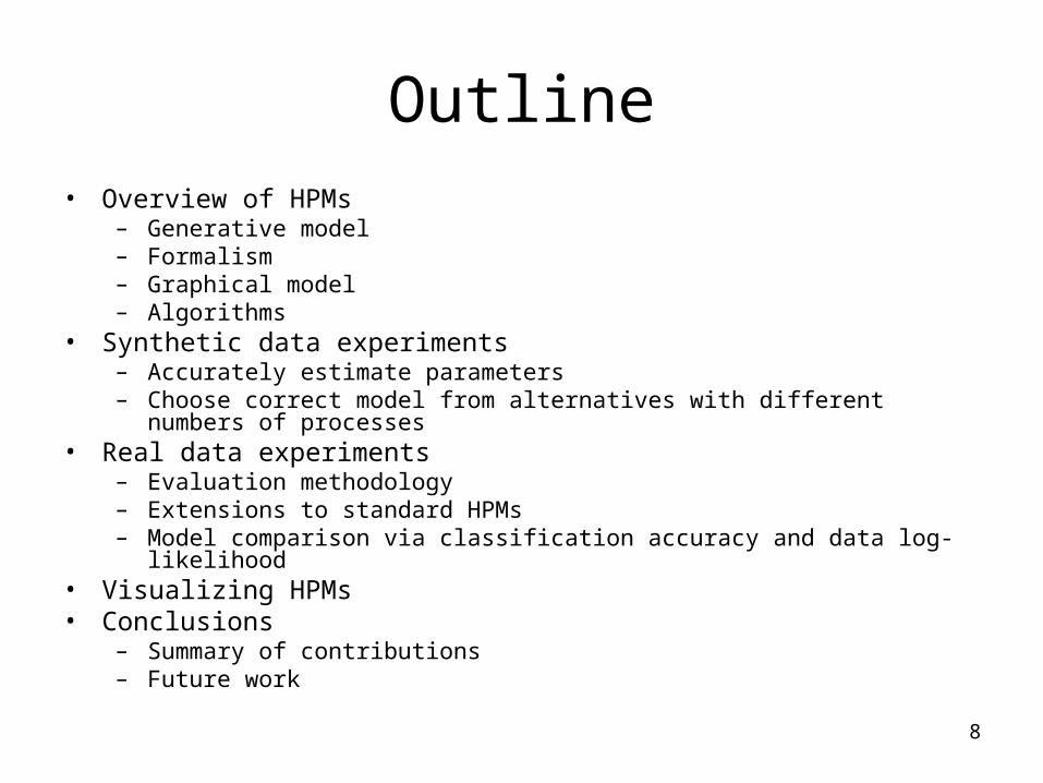
Outline• Overview of HPMs
– Generative model– Formalism– Graphical model– Algorithms
• Synthetic data experiments– Accurately estimate parameters– Choose correct model from alternatives with different numbers of processes
• Real data experiments– Evaluation methodology– Extensions to standard HPMs– Model comparison via classification accuracy and data log-likelihood
• Visualizing HPMs• Conclusions
– Summary of contributions– Future work
9
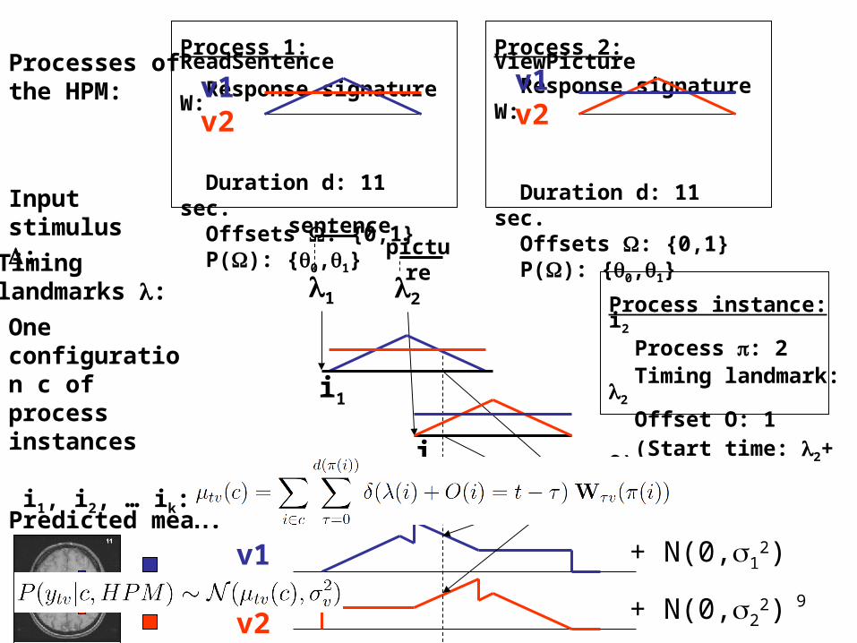
Process 1: ReadSentence Response signature W:
Duration d: 11 sec. Offsets : {0,1} P(): {0,1}
One configuration c of process instances i1, i2, … ik:
Predicted mean:
Input stimulus :
i1
Timing landmarks : 21
i2
Process instance: i2 Process : 2 Timing landmark: 2
Offset O: 1 (Start time: 2+ O)
sentencepicture
v1v2
Process 2: ViewPicture Response signature W:
Duration d: 11 sec. Offsets : {0,1} P(): {0,1}
v1v2
Processes of the HPM:
v1
v2
+ N(0,12)
+ N(0,22)
10
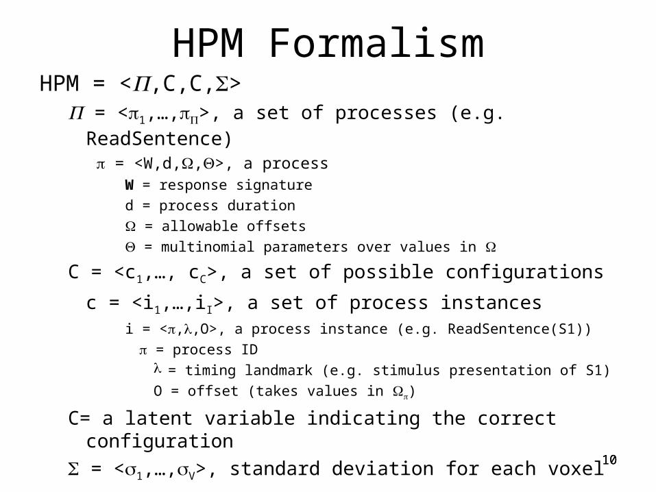
HPM FormalismHPM = <,C,C,>
= <1,…,>, a set of processes (e.g. ReadSentence)
= <W,d,,>, a processW = response signature
d = process duration
= allowable offsets
= multinomial parameters over values in
C = <c1,…, cC>, a set of possible configurations
c = <i1,…,iI>, a set of process instances i = <,,O>, a process instance (e.g. ReadSentence(S1))
= process ID = timing landmark (e.g. stimulus presentation of S1)
O = offset (takes values in )
C= a latent variable indicating the correct configuration
= <1,…,V>, standard deviation for each voxel10
11
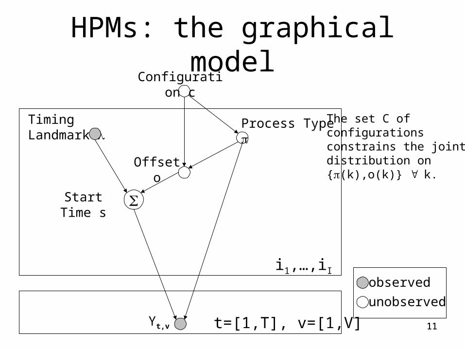
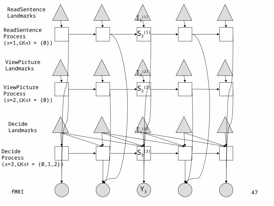
HPMs: the graphical model
Offset o
Process Type
Start Time s
observed
unobserved
Timing Landmark
Yt,v
i1,…,iI
t=[1,T], v=[1,V]
The set C of configurations constrains the joint distribution on {(k),o(k)} k.
Configuration c
11
12
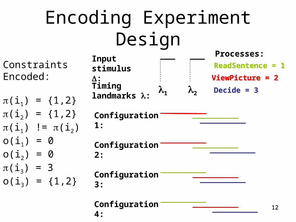
Encoding Experiment Design
Configuration 1:
Input stimulus :
Timing landmarks :
21
ViewPicture = 2
ReadSentence = 1
Decide = 3
Configuration 2:
Configuration 3:
Configuration 4:
Constraints Encoded:
(i1) = {1,2}(i2) = {1,2}(i1) != (i2)o(i1) = 0o(i2) = 0(i3) = 3o(i3) = {1,2}
Processes:
12
ViewPicture = 2
ReadSentence = 1
Decide = 3
ViewPicture = 2
ReadSentence = 1
13
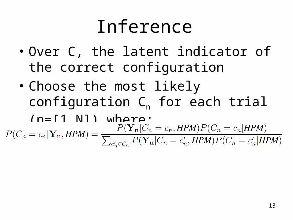
Inference• Over C, the latent indicator of the correct
configuration
• Choose the most likely configuration Cn for each trial (n=[1,N]) where:
13
14
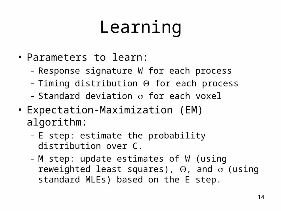
Learning
• Parameters to learn:– Response signature W for each process– Timing distribution for each process – Standard deviation for each voxel
• Expectation-Maximization (EM) algorithm:– E step: estimate the probability distribution over C.– M step: update estimates of W (using reweighted
least squares), , and (using standard MLEs) based on the E step.
14
15
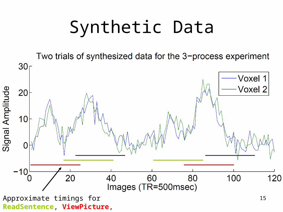
Synthetic Data
Approximate timings for ReadSentence, ViewPicture, Decide
16
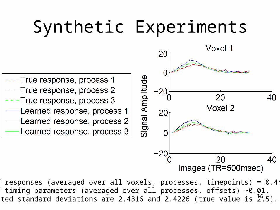
Synthetic Experiments
MSE of responses (averaged over all voxels, processes, timepoints) = 0.4427.MSE of timing parameters (averaged over all processes, offsets) ~0.01.Estimated standard deviations are 2.4316 and 2.4226 (true value is 2.5).
17
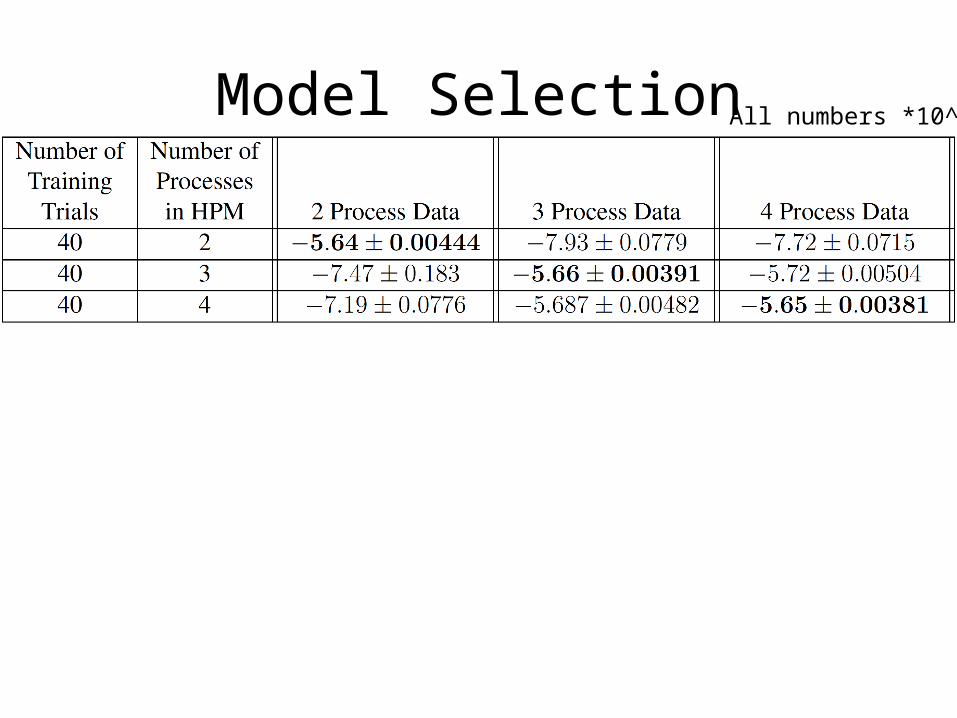
Model Selection All numbers *10^5
18
Synthetic Data Results
• Tracking processes: HPMs can recover the parameters of the model used to generate the data.
• Comparing models: HPMs can use held-out data log-likelihood to identify the model with the correct number of latent processes.
19
Evaluating HPMs on real data
• No ground truth for the problems HPMs were designed for.
• Can use data log-likelihood to compare– Baseline: average of all training trials
• Can do classification of known entities (like the stimuli), but HPMs are not optimized for this.
20
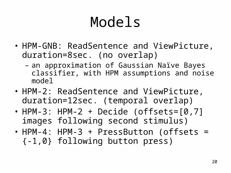
Models
• HPM-GNB: ReadSentence and ViewPicture, duration=8sec. (no overlap)– an approximation of Gaussian Naïve Bayes classifier,
with HPM assumptions and noise model
• HPM-2: ReadSentence and ViewPicture, duration=12sec. (temporal overlap)
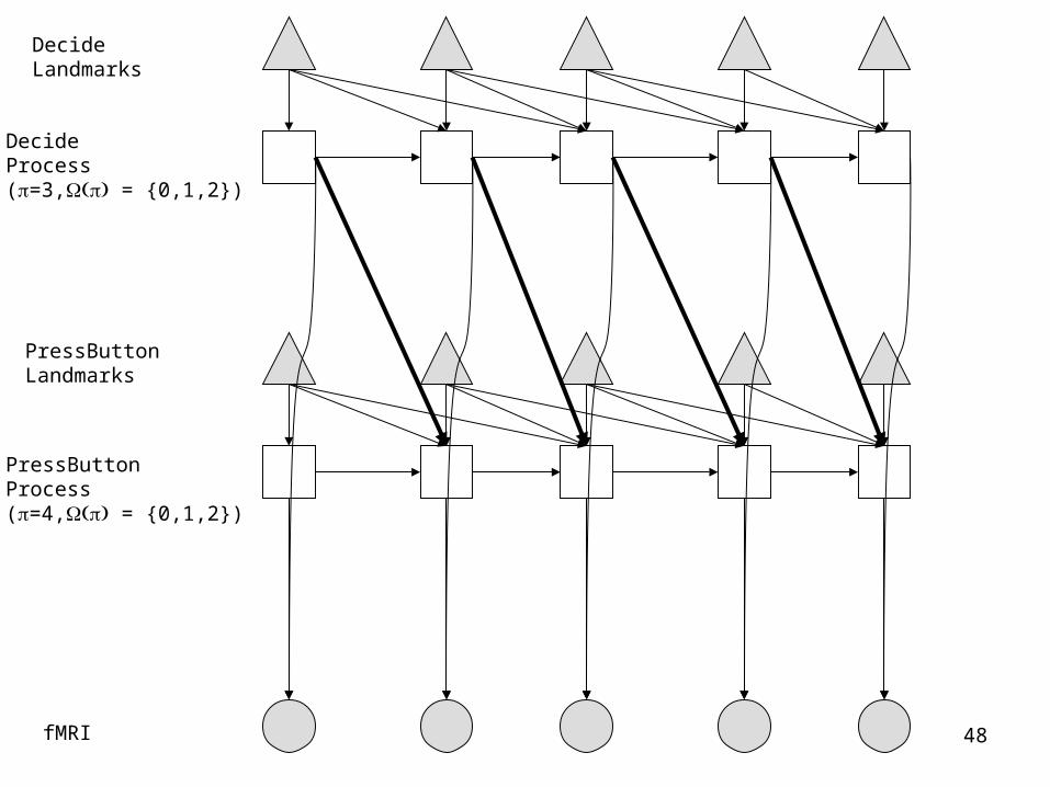
• HPM-3: HPM-2 + Decide (offsets=[0,7] images following second stimulus)
• HPM-4: HPM-3 + PressButton (offsets = {-1,0} following button press)
21
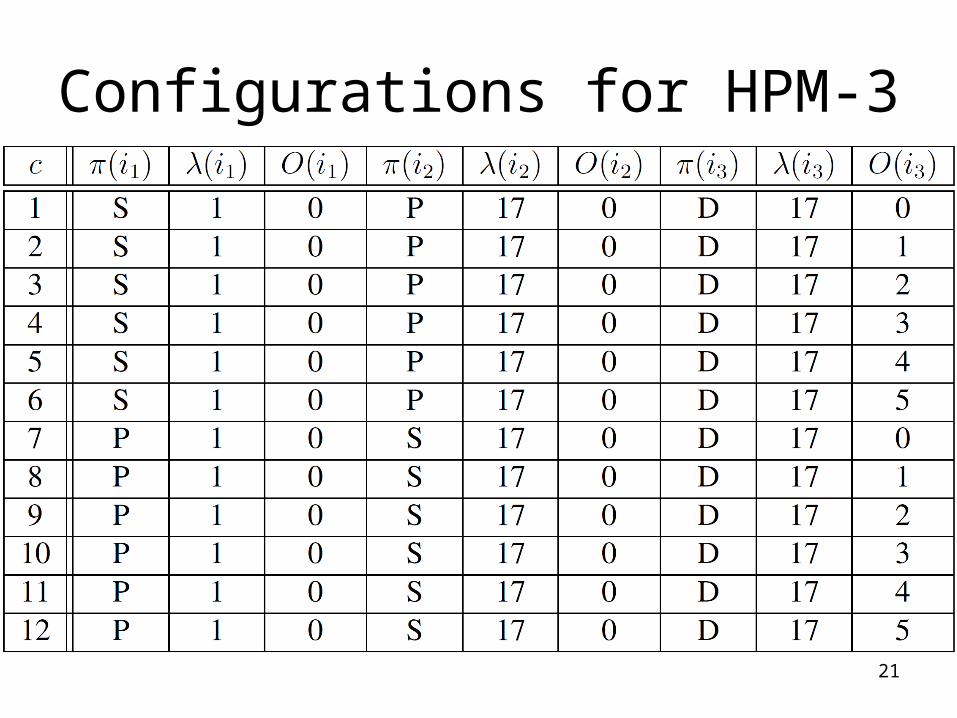
Configurations for HPM-3
22
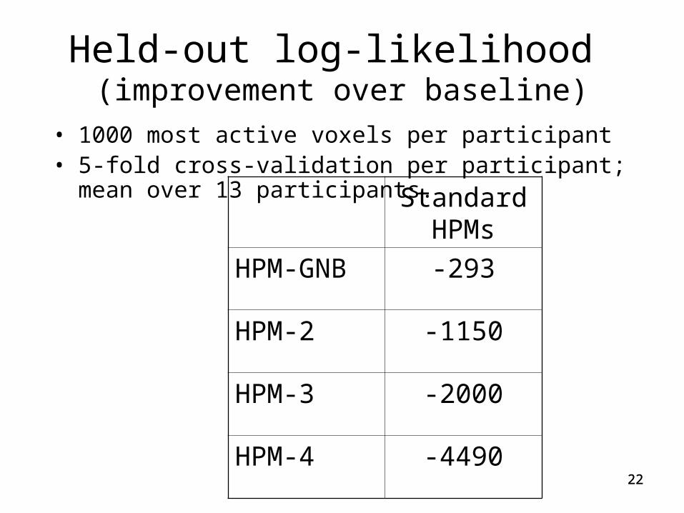
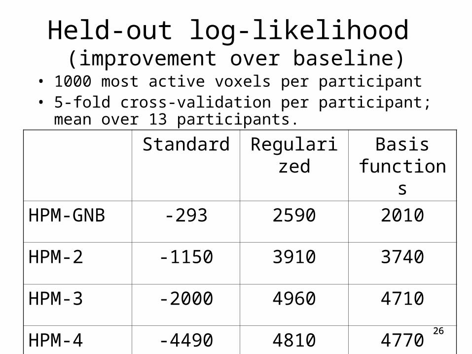
Held-out log-likelihood (improvement over baseline)
• 1000 most active voxels per participant• 5-fold cross-validation per participant; mean over 13
participants. Standard HPMs
HPM-GNB -293
HPM-2 -1150
HPM-3 -2000
HPM-4 -449022
23
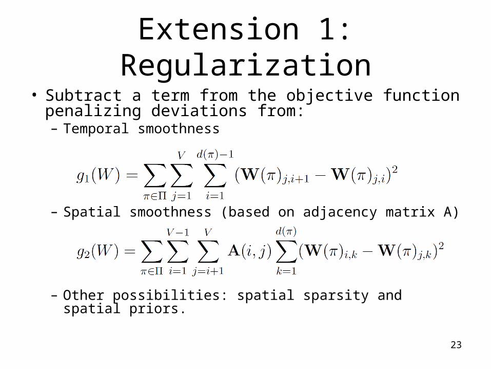
Extension 1: Regularization
• Subtract a term from the objective function penalizing deviations from:– Temporal smoothness
– Spatial smoothness (based on adjacency matrix A)
– Other possibilities: spatial sparsity and spatial priors.
24
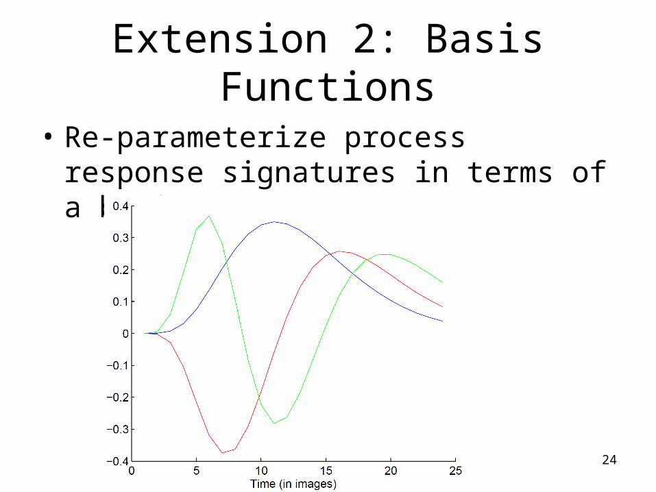
Extension 2: Basis Functions
• Re-parameterize process response signatures in terms of a basis set
25
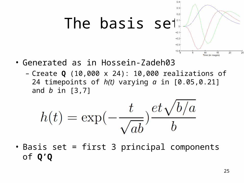
The basis set
• Generated as in Hossein-Zadeh03– Create Q (10,000 x 24): 10,000 realizations of 24
timepoints of h(t) varying a in [0.05,0.21] and b in [3,7]
• Basis set = first 3 principal components of Q’Q
26
Held-out log-likelihood (improvement over baseline)
• 1000 most active voxels per participant• 5-fold cross-validation per participant; mean over 13
participants.
Standard Regularized Basis functions
HPM-GNB -293 2590 2010
HPM-2 -1150 3910 3740
HPM-3 -2000 4960 4710
HPM-4 -4490 4810 477026
27
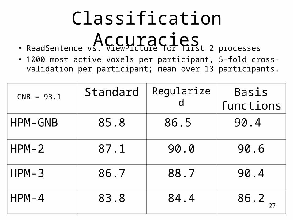
Classification Accuracies• ReadSentence vs. ViewPicture for first 2 processes• 1000 most active voxels per participant, 5-fold cross-
validation per participant; mean over 13 participants.
Standard Regularized Basis functions
HPM-GNB 85.8 86.5 90.4
HPM-2 87.1 90.0 90.6
HPM-3 86.7 88.7 90.4
HPM-4 83.8 84.4 86.2
GNB = 93.1
28
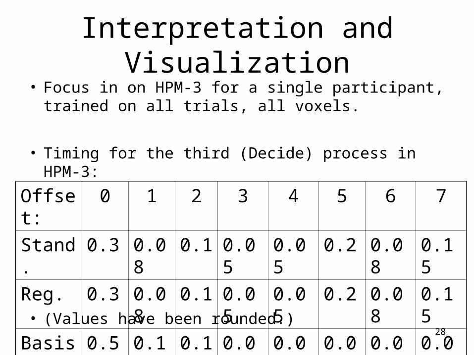
Interpretation and Visualization• Focus in on HPM-3 for a single participant,
trained on all trials, all voxels.
• Timing for the third (Decide) process in HPM-3:
• (Values have been rounded.)
Offset: 0 1 2 3 4 5 6 7
Stand. 0.3 0.08 0.1 0.05 0.05 0.2 0.08 0.15
Reg. 0.3 0.08 0.1 0.05 0.05 0.2 0.08 0.15
Basis 0.5 0.1 0.1 0.08 0.05 0.03 0.05 0.08
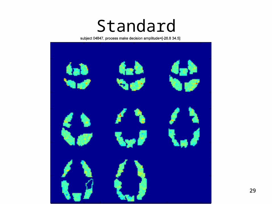
29
Standard
29
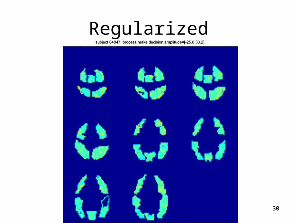
30
Regularized
30

31
Basis functions
31
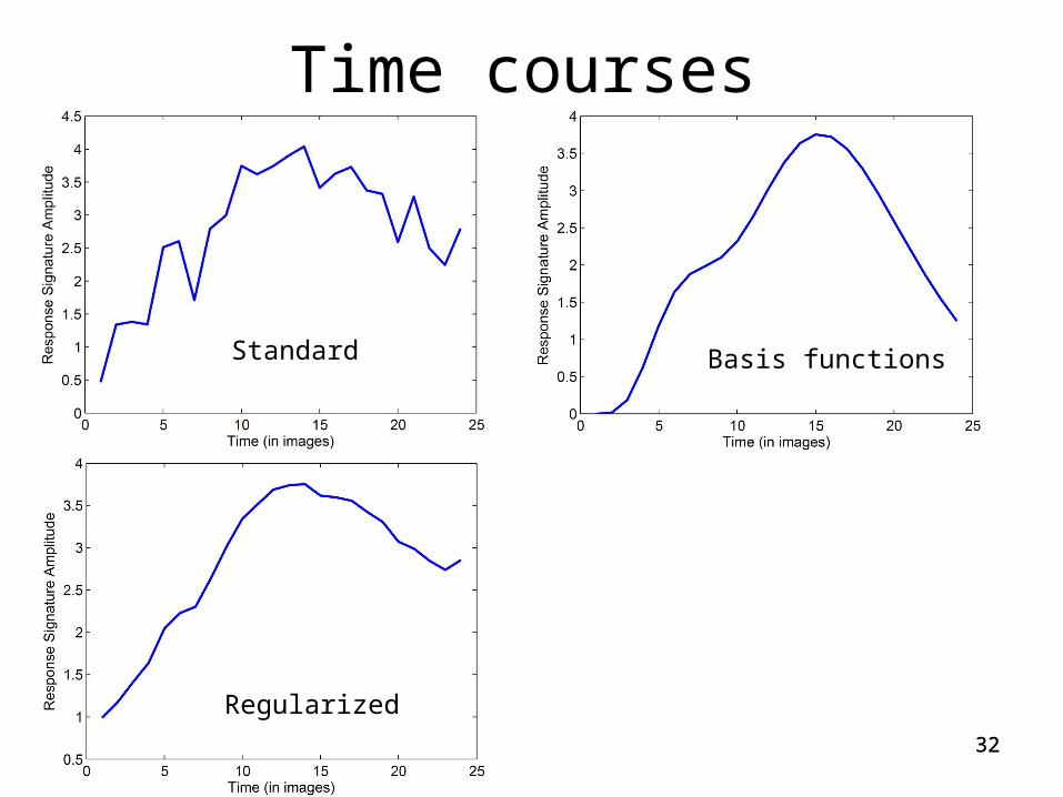
32
Time courses
Standard
Regularized
Basis functions
32
33
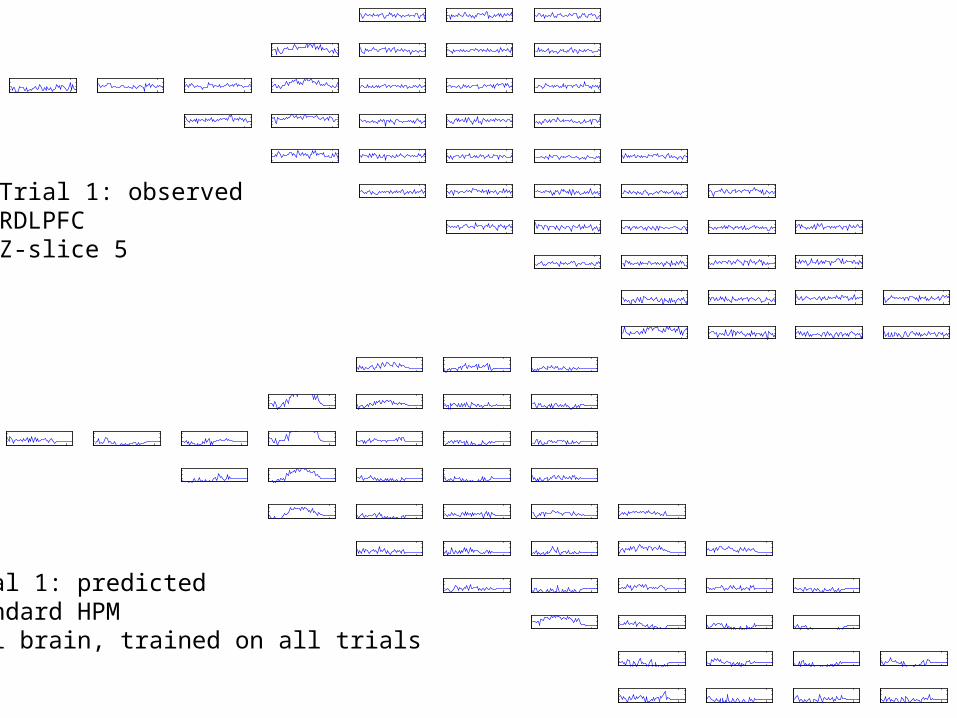
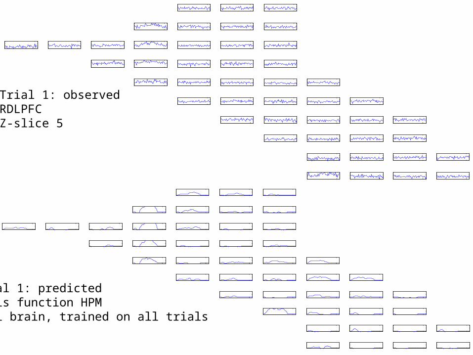
Trial 1: observedRDLPFCZ-slice 5
Trial 1: predictedStandard HPMFull brain, trained on all trials
34
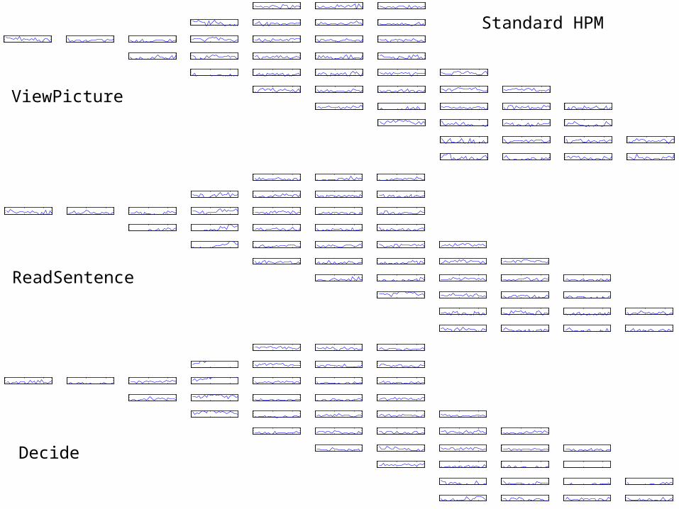
ViewPicture
ReadSentence
Decide
Standard HPM
35
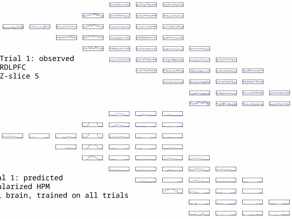
Trial 1: observedRDLPFCZ-slice 5
Trial 1: predictedRegularized HPMFull brain, trained on all trials
36
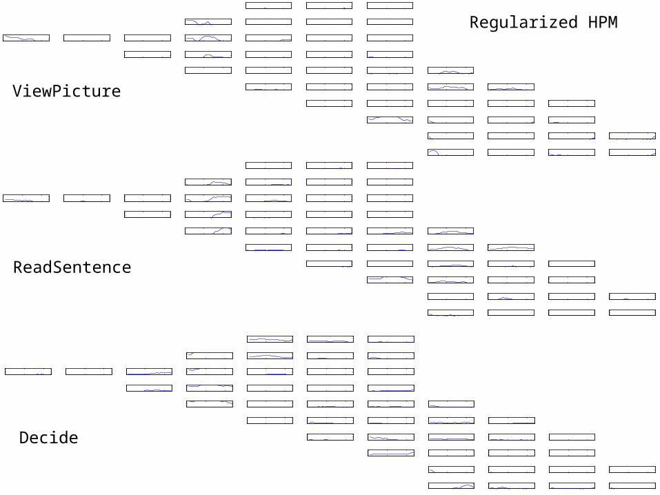
ViewPicture
ReadSentence
Decide
Regularized HPM
37
Trial 1: observedRDLPFCZ-slice 5
Trial 1: predictedBasis function HPMFull brain, trained on all trials
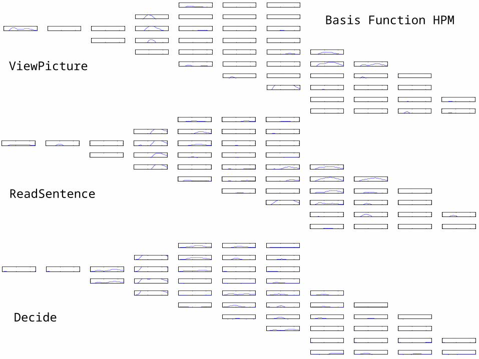
38
ViewPicture
ReadSentence
Decide
Basis Function HPM
39
Caveats
• While visualizing these parameters can help us understand the model, it is important to remember that they are specific to the design choices of the particular HPM.
• These are parameters – not the results of statistical significance tests.
40
Summary of Results
• Synthetic data results – HPMs can recover the parameters of the model
used to generate the data in an ideal situation.– We can use held-out data log-likelihood to
identify the model with the correct number of latent processes.
• Real data results – Standard HPMs can overfit on real fMRI data.– Regularization and HPMs parameterized with
basis functions consistently outperform the baseline in terms of held-out data log-likelihood.
– Example comparison of 4 models.
41
Contributions
• Estimates for Decide!
• To our knowledge, HPMs are the first probabilistic model for fMRI data that can estimate the hemodynamic response for overlapping mental processes with unknown onset while simultaneously estimating a distribution over the timing of the processes.
42
Future Directions
• Combine regularization and basis functions.• Develop a better noise model.• Relax the linearity assumption.• Automatically discover the number of latent
processes.• Learn process durations.• Continuous offsets.• Leverage DBN algorithms.
43
ReferencesJohn R. Anderson, Daniel Bothell, Michael D. Byrne, Scott Douglass, Christian Lebiere, and Yulin Qin. An integrated theory of the mind. Psychological Review, 111(4):1036–1060, 2004. http://act-r.psy.cmu.edu/about/.
Anders M. Dale. Optimal experimental design for event-related fMRI. Human Brain Mapping, 8:109–114, 1999.
Zoubin Ghahramani and Michael I. Jordan. Factorial hidden Markov models. Machine Learning, 29:245–275, 1997.
John-Dylan Haynes and Geraint Rees. Decoding mental states from brain activity in humans. Nature Reviews Neuroscience, 7:523–534, July 2006.
Gholam-Ali Hossein-Zadeh, Babak A. Ardekani, and Hamid Soltanian-Zadeh. A signal subspace approach for modeling the hemodynamic response function in fmri. Magnetic Resonance Imaging, 21:835–843, 2003.
Marcel Adam Just, Patricia A. Carpenter, and Sashank Varma. Computational modeling of high-level cognition and brain function. Human Brain Mapping, 8:128–136, 1999. http://www.ccbi.cmu.edu/project 10modeling4CAPS.htm.
Tim A. Keller, Marcel Adam Just, and V. Andrew Stenger. Reading span and the timecourse of cortical activation in sentence-picture verification. In Annual Convention of the Psychonomic Society, 2001.
Kevin P. Murphy. Dynamic bayesian networks. To appear in Probabilistic Graphical Models, M. Jordan, November 2002.
43

44
Thank you!

45
Questions?
46
(end of talk)
47
ReadSentence Landmarks
ReadSentence Process(=1, = {0})
ViewPicture Landmarks
ViewPicture Process(=2, = {0})
DecideLandmarks
Decide Process(=3, = {0,1,2})
fMRI
I3(1)
S3(1)
S3(2)
I3(2)
I3(3)
S3(3)
Y3
48
PressButtonLandmarks
PressButton Process(=4, = {0,1,2})
DecideLandmarks
fMRI
Decide Process(=3, = {0,1,2})