Universidade de Sao Paulo

Instituto de Fısica

Hidrodinamica Evento-por-eventopara o LHC

Meera Vieira Machado

Orientador: Prof.a Dra. Frederique Marie Brigitte Sylvie Grassi

Dissertacao de Mestrado apresentada ao Instituto deFısica, Universidade de Sao Paulo, para a obtencao do

tıtulo de Mestre em Ciencias

Banca Examinadora:

Prof.a Dra. Frederique Marie Brigitte Sylvie Grassi (IFUSP)Prof. Dr. Fernando Silveira Navarra (IFUSP)Prof.a Dra. Sandra dos Santos Padula (IFT/UNESP)

Sao Paulo2015

FICHA CATALOGRÁFICA

Preparada pelo Serviço de Biblioteca e Informação

do Instituto de Física da Universidade de São Paulo

Machado, Meera Vieira Hidrodinâmica evento-por-evento para o LHC / Event-by-event hydrodynamics for LHC. São Paulo, 2015. Dissertação (Mestrado) – Universidade de São Paulo. Instituto de Física. Depto. Física Matemática. Orientador: Profa. Dra. Frederique Grassi Área de Concentração: Física de Altas Energias. Unitermos: 1. Hidrodinâmica; 2. LHC; 3. Colisões de íons pesados; 4. Evento-por-evento. USP/IF/SBI-078/2015

Universidade de Sao Paulo

Instituto de Fısica

Event-by-event Hydrodynamicsfor LHC

Meera Vieira Machado

Supervisor: Prof. Dr. Frederique Marie Brigitte Sylvie Grassi

Masters dissertation submitted to the PhysicsInstitute, University of Sao Paulo, in partial fulfillmentof the requirements for the degree of Master of Sciences

Examination Committee:

Prof. Dr. Frederique Marie Brigitte Sylvie Grassi (IFUSP)Prof. Dr. Fernando Silveira Navarra (IFUSP)Prof. Dr. Sandra dos Santos Padula (IFT/UNESP)

Sao Paulo2015

Acknowledgments

First and foremost, I would like to thank my parents Maria Zuleide Vieira de Sousa andJose Wagner Borges Machado and my grandmother Rosa Vieira de Sousa for the endless sup-port on my studies. Secondly, to Elmar van Cleynenbreugel, for providing me with love andfriendship through the last two years. I am also grateful for my family in Brasılia and Ceara,for giving me courage and be always there rooting for me, even being so far away. I appreciatethe long term support and companionship of my friends in Brasilia, who have been with methrough my child and adulthood, always offering a hand whenever I needed help.

From Sao Paulo, I would like to thank my friends in the Mathematical Physics Department(IFUSP), specially Arthur Eduardo da Mota Loureiro, for providing me with new insights inphysics and even philosophy of science and being the closest I had to a family in this city. Iam grateful to Thiago Razseja, Javier Lorca, Pablo Ibieta and Alessandra Brognara for theirfriendship when we had all just arrived.

I thank my office colleagues Leonardo de Avellar and Tania Torrejon for the interestingdiscussions on physics and other matters and for coping with me through these years.

I thank my supervisor, Prof. Dr. Frederique Grassi, for being patient and orienting methrough this whole process, thus providing me with way more knowledge on science researchthan I had before. I also thank Professor Fernando Gardim and Dr. Danuce Dudek for the nu-merous discussions on the NexSPheRIO code, which helped a lot with my research. My thanksto Dr. Jacquelyn Noronha-Hostler, who not only provided me with her numerical codes, butalso taught me a lot about harmonic flows and other observables. I am grateful to Prof. SandraPadula for adding me to her IFT project so that I could make also use of UNESP’s compu-tational power. I thank Prof. Yogiro Hama for the brief, yet useful discussions on heavy-ioncollisions and Prof. Wei-Liang Qian for helping me with NexSPheRIO.

I am truly grateful for the numerical support team of IFUSP, Prof. Jorge de Lyra andJoao Borges, without whom I would not have been able to perform such extensive numericalcalculations and the NCC and Grid-UNESP personnel, for letting me use their computationalpower to also run the NexSPheRIO code.

I would also like to thank the Mathematical Physics Department’s secretaries Amelia Gen-ova, Cecilia Blanco and Simone Shinomiya for having done so much for me during all thoseyears, as well as the CPG-IFUSP personnel, specially Andrea Wirkus, Eber De Patto Lima,Paula Mondini and Claudia Conde for the attention and help with all the necessary procedures.

At last, I thank CNPq for the financial support.

v

Resumo

E feita uma analise de hidrodinamica evento-por-evento para colisoes de Pb-Pb a energiaincidente de

√sNN = 2.76 TeV. Estudamos os efeitos de duas equacoes de estado sob as

mesmas condicoes iniciais e desacoplamento: uma e caracterizada por um ponto crıtico e aoutra e baseada em calculos de Lattice QCD (Cromodinamica Quantica). Os observaveis deinteresse sao os espectros de partıculas em termos da pseudo rapidez e momento transversal,assim como os coeficientes harmonicos de Fourier que, por sua vez, carregam as anisotropiasiniciais do sistema durante toda a sua evolucao. Tais observaveis sao calculados e comparadoscom dados experimentais do Large Hadron Collider (LHC). Por fim, os calculos baseados emparametros referentes as energias do LHC sao comparados com trabalhos anteriores feitos combase em dados experimentais do Relativistic Heavy-Ion Collider (RHIC). Os principais metodosusados no caso anterior sao aplicados a este trabalho, o que resulta em algumas diferencas entreos resultados dos dois tipos de colisao, desde a distribuicao de energia inicial a temperaturasde freeze-out.

vi

Abstract

We perform an event-by-event hydrodynamic analysis for Pb-Pb collisions at the incidentenergy of

√sNN = 2.76 TeV, also studying the effects of two equations of state under the

same initial conditions and freeze-out scenario: one characterized by a critical point and theother based on Lattice QCD (Quantum Chromodynamics) calculations. The observables ofinterest are particle spectra in terms of pseudorapidity and transverse momentum, as well asflow harmonics, which are coefficients that carry information on the initial anisotropies of thesystem throughout its evolution. Those are computed and compared with experimental LargeHadron Collider (LHC) data. There are slight differences in the results for each equation ofstate, caused by their distinct features. Lastly, the LHC-based calculations are compared withprevious works related to the Relativistic Heavy-Ion Collider (RHIC) experimental data. Themain techniques of the latter are performed in this work, which results in differences betweensome aspects in the outcome for each collision type, from initial energy distributions to freeze-out temperatures.

vii

Summary

1 Introduction 1

2 Hydrodynamics and the Collision 32.1 The Equations of Motion . . . . . . . . . . . . . . . . . . . . . . . . . . . . . . . 32.2 Initial Conditions . . . . . . . . . . . . . . . . . . . . . . . . . . . . . . . . . . . 62.3 Equations of State . . . . . . . . . . . . . . . . . . . . . . . . . . . . . . . . . . 8

2.3.1 Equation of State with Critical Point (CPEoS) . . . . . . . . . . . . . . . 82.3.2 Lattice QCD Equation of State (LattEoS) . . . . . . . . . . . . . . . . . 152.3.3 Comparison between EoS . . . . . . . . . . . . . . . . . . . . . . . . . . 17

2.4 Cooper-Frye Decoupling Mechanism . . . . . . . . . . . . . . . . . . . . . . . . . 18

3 On NexSPheRIO 213.1 The SPH Method . . . . . . . . . . . . . . . . . . . . . . . . . . . . . . . . . . . 213.2 Decoupling in SPH . . . . . . . . . . . . . . . . . . . . . . . . . . . . . . . . . . 273.3 The Code’s Structure . . . . . . . . . . . . . . . . . . . . . . . . . . . . . . . . . 28

4 Results 304.1 Centrality Classes . . . . . . . . . . . . . . . . . . . . . . . . . . . . . . . . . . . 304.2 Particle Spectra . . . . . . . . . . . . . . . . . . . . . . . . . . . . . . . . . . . . 32

4.2.1 Pseudorapidity Distribution . . . . . . . . . . . . . . . . . . . . . . . . . 334.2.2 Transverse Momentum Distribution . . . . . . . . . . . . . . . . . . . . . 36

4.3 Flow Analysis . . . . . . . . . . . . . . . . . . . . . . . . . . . . . . . . . . . . . 394.3.1 Event Plane Method . . . . . . . . . . . . . . . . . . . . . . . . . . . . . 404.3.2 Results . . . . . . . . . . . . . . . . . . . . . . . . . . . . . . . . . . . . . 40

4.4 Comparison with RHIC . . . . . . . . . . . . . . . . . . . . . . . . . . . . . . . 50

5 Conclusion 56

A Energy-momentum Tensor in any Reference Frame 58

B Coordinates in Heavy-Ion Collisions 60

C Relativistic Fluid’s Action in a General Coordinate System 62

References 67

viii

Chapter 1

Introduction

The Big Bang theory is one of the most accepted explanations to the beginning of theUniverse. Proposed by LeMaıtre, the latter would have expanded from a state of high energydensity and extreme temperatures. Due to said conditions and the relative small distances, it isbelieved that millionths of seconds after the Big Bang, quarks and gluons were asymptoticallyfree. Such state of matter is denoted Quark-Gluon Plasma. In the year of 2000, the EuropeanOrganization for Nuclear Research (CERN) officially announced[1] that compelling evidencefor the existence of a new state of matter had been found. This followed the analysis of manyexperimental data collected during 15 years of heavy-ion experiments at the Super Proton Syn-chrotron (SPS).

In the same year, the Relativistic Heavy-Ion Collider (RHIC) started accelerating goldatoms to a center-of-mass energy several times higher than before, reaching up to 200 AGeV inthe following years. Later on, Brookhaven National Laboratory claimed to have come upon amedium where the relevant degrees of freedom, over nuclear volumes, are those of quarks andgluons, rather than of hadrons[2]. Such is the Quark-Gluon Plasma, a strongly interacting lowviscosity fluid.

Built to smash lead atoms at even higher energies (2.76 ATeV) than its predecessors, theLarge Hadron Collider (LHC) is the present of ultra-relativistic heavy ion collisions. Studiesof the experimental data collected by the ALICE (A Large Ion Collider Experiment), CMS(Compact Muon Solenoid) and ATLAS (A Toroidal LHC Apparatus) detectors should givenew insight on the QGP properties and perhaps even give signs of new physics.

When studying the collisions of heavy-ions, one should analyze each step separately. Firstthe nuclei collide at relativistic energies, meaning that they are Lorentz contracted in the beamdirection by a factor of γ = (1− v2)−1/2, where v is their velocity in the laboratory frame. Atsuch extreme temperature and energy density values, the Quark-Gluon Plasma is thus formed.The great pressure difference between its core and the vacuum surrounding it makes the QGPsuffer an explosive collective expansion, eventually undergoing a phase transition to a purehadronic state as the temperature cools down. At last, the produced hadrons reach the de-tectors, which is the only piece of concrete information that theoreticians and experimentalistshave to study the whole evolution that precedes this final moment.

Reconstructing the steps of a heavy-ion expansion is no easy task and many models havebeen formulated throughout the years. Enrico Fermi was the first to propose the fruitful idea

1

of considering the formed matter in thermal equilibrium and apply statistical methods to itsstudy[3]. His model was based on the statistical weights of each particle species and it failedto explain the high abundance of pions in relation to kaons. Following the former’s main ideaon thermal equilibrium, Landau suggested that matter expands according the hydrodynamicequations of motion before hadron emission occurs[4, 5]. From then on, the latter has beenextensively applied in the realm of relativistic heavy-ion collisions, alongside with models ofinitial conditions, equations of state and freeze-out scenarios.

In this work we apply event-by-event hydrodynamics to simulate Pb-Pb collisions at√sNN = 2.76 TeV and compare the resultant observables with LHC data from the ALICE,

CMS and ATLAS detectors. We begin by presenting the necessary ingredients for the calcu-lation: first, we outline the hydrodynamic equations of motion in section 2.1, followed by ananalysis of the initial conditions generated by Nexus[6] at such high energies. Two equationsof state are then discussed as well as the system’s freeze-out mechanism.

With the main parts set, we proceed on employing the Smoothed-Particle Hydrodynamics(SPH) method to solve the hydrodynamic equations of motion using the variational princi-ple. The aforementioned is the core of the Smoothed-Particle hydrodynamic evolution ofRelativistic Heavy-IOn collisions (SPheRIO)[7, 8] numerical code; its outline is the subject ofsection 3.3.

Finally, we compare the results to some heavy-ion collision observables, such as chargedparticle production in terms of pseudorapidity and transverse momentum as well as flowanisotropies, lastly comparing them with previous works on RHIC, where we discuss the mainsimilarities and differences between them.

2

Chapter 2

Hydrodynamics and the Collision

2.1 The Equations of Motion

It was previously stated that relativistic hydrodynamics can describe the dynamics of theexpansion that follows a heavy-ion collision, due to the collective behavior of the producedmatter. Hydrodynamics is a long-distance description of what can be either a classical or aquantum many-body system [9]. Therefore, the phenomena considered in such dynamics aremacroscopic, meaning that a fluid is seen as a continuous medium [10]. Any infinitesimalfluid element is still large compared to the distance between the molecules in it. That is thecontinuum hypothesis. Such assumption implies that the typical scale of the hydrodynamicvariables is way larger than the microscopic scale defined by the interactions between the fluidcomponents[11]. Local thermodynamic equilibrium, the condition upon hydrodynamic relies,may thus prevail[12].

In order to obtain the equations of motion of relativistic hydrodynamics, it is necessaryto inquire deeper into the conservation laws governing it. According to Noether’s theorem,continuous symmetries in a theory lead to conserved quantities, which imply the existence ofconserved currents [9]. For the case at hand, there is symmetry in spacetime translation, whichleads to the conservation of total energy and momentum, whose associated conserved currentsare the energy-momentum tensor T µν . Additionally, the fluid may carry other conserved quan-tities such as baryon number or charge [13]. In the relativistic case, the number of particles isnot conserved, since the energy is high enough for particle creation and annihilation to occur.The conservation of baryon number, for instance, leads to the conserved current Jµ. Thus weshall have:

∂µTµν = 0, (2.1)

∂µJµ = 0. (2.2)

These are the conservation laws of a system described by relativistic hydrodynamics.

We shall consider the fluid in Minkowski space with metric ηµν = diag(1,−1,−1,−1) aswell as c = ~ = kb = 1. Its 4-velocity is defined by uµ = dxµ

dτ, where τ is the proper time and

xµ(τ) is the trajectory of the fluid element. Hence, taking uµ = (u0, ~u) we must have:

3

u0 =dx0

dτ= γ,

~u =dx

dτ= γ~v, (2.3)

where γ = 1√1−~v2 is the Lorentz Factor and ~v is the velocity of a fluid element with respect

to the laboratory rest frame. Consequently, the fluid velocity is normalized, uµuµ = u20−~u2 = 1.

As it was previously mentioned, the assumption of local thermodynamic equilibrium isvalid for the system at hand. That means the fluid element has isotropic properties in its restframe. For instance, energy and momentum flux are zero. A nonzero current would define adirection in space, violating isotropy [11, 12]. In ideal hydrodynamics, baryon flux must bezero in the proper frame[12].

We define the conserved current Jµ = (n0, ~n), with n0 as the baryon number density and ~nas the baryon flux. If n is the baryon number density in the fluid’s rest frame, then JµRF = (n, 0).In order to obtain Jµ in a moving frame, it is necessary to do a Lorentz Transformation:

Jµ = ΛµνJ

νRF . (2.4)

Since Λµν = ∂x′µ

∂xν:

Λ00 = γ Λi

0 = γvi

Λ0j = −γvj Λi

j = δij + vivjγ − 1

v2, (2.5)

with Λ0j and Λi

j conveniently chosen[13]. Therefore:

J0 = Λ0νJ

νRF = Λ0

0J0RF + Λ0

iJiRF = γn,

J i = ΛiνJ

νRF = Λi

0J0RF + Λi

jJjRF = γnvi,

⇒ Jµ = (γn, γnvi)

⇒ Jµ = nuµ. (2.6)

From ∂µJµ = 0 and equation (2.6) above:

∂µJµ = ∂µnu

µ = 0,

∂(nγ)

∂t+∇ · (nγ~v) = 0, (2.7)

which is the continuity equation.

It is worth remarking that Jµ = nuµ is the simplest 4-vector we can write with the quan-tities n and uµ, without accounting for their derivatives.

4

The conserved currents associated with energy-momentum conservation can be written asa tensor T µν , where each value of ν indicates a component of the 4-momentum and µ corre-sponds to components of the conserved current [12]. Having established that, T 00 becomes theenergy density, T 0j is the momentum density, T i0 the energy flux along axis i and T ij formsthe momentum flux density tensor – also known as pressure tensor [10, 12].

Firstly, we shall define T µν in the fluid’s proper frame. The components associated withmomentum density and energy flux, T 0j and T i0, thus disappear. T 00 = ε, where ε is the properenergy density. Since Pascal’s Law is valid in this case, T ijdaj – momentum flux through asurface element daj – equals the pressure acting in such surface, Pdaj. Hence, T ij = Pδij andT µν acquires the form:

T µνRF =

ε 0 0 00 P 0 00 0 P 00 0 0 P

. (2.8)

Secondly, consider an inertial frame in which the fluid appears to be moving with velocity~v. Under a Lorentz transformation T µν shall be written as:

T µν = ΛµαΛν

βTαβRF . (2.9)

Using equations (2.5) in the expression above (see Appendix A), we finally arrive at T µν ’sexpression for ideal fluids at an arbitrary speed, ~v:

T µν = (ε+ P )uµuν − Pηµν . (2.10)

It is worth noticing that T µν = T νµ.

Under the perfect fluid hypothesis, the energy-momentum tensor and baryonic currenttake the forms depicted as equations (2.6) and (2.10). ε = ε(x), P = P (x), uµ = uµ(x) andn = n(x) are promoted to slowly varying fields. Additionally, an equilibrium equation of statesupplies one with P (T, µ), from which the thermodynamic relations s = ∂P

∂T, n = ∂P

∂µand

ε = −P + Ts+ µn evaluate ε,n and s – entropy density [9].

Given equation (2.1), the projection of T µν in the four-velocity’s direction shall be uν∂µTµν =

0. Thus:

uν∂µ[(ε+ P )uµuν ]− uν∂µPηµν = 0

.Recalling that uµuµ = 1,

∂µ[(ε+ P )uµ] + (ε+ P )uµuν∂µuν − uµ∂µP = 0

.Since uν∂µu

ν = 0, one shall have:

∂µ(ε+ P )uµ + (ε+ P )∂µuµ − uµ∂µP = 0

⇒ uµ∂µε+ (ε+ P )∂µuµ = 0

⇒ uµ∂µ(−P + Ts+ µn) + (Ts+ µn)∂µuµ = 0.

5

Equation (2.2) and ∂µP = s∂µT + n∂µµ yield:

T (uµ∂µs+ s∂µuµ) = 0

⇒ ∂µ(suµ) = 0, (2.11)

which is the conservation of entropy density current, sµ = suµ. Locally, entropy does notincrease in ideal hydrodynamics [9]. Hence:

∂µTµν = 0 ∂µJ

µ = 0

with the conserved currents defined as:

Jµ = nuµ

T µν = (ε+ P )uµuν − Pηµν

consist in the Equations of Motion of Relativistic Ideal Hydrodynamics (EoM). Combined withthe equation of state, P (T, µ) they form a closed system of equations.

2.2 Initial Conditions

The first stage in solving the hydrodynamic equations is setting their initial (IC) andboundary conditions. The latter demand that energy density and other thermodynamic vari-ables tend to zero at large distances from the collision center or, in the case of a boost-invariantsystem, the collision axis[14].

When the nuclei collide, particles are created and they interact with each other throughcomplex processes not completely understood. One then assumes that the system eventuallyreaches local thermodynamic equilibrium, since hydrodynamics strongly relies on such assump-tion. Having said that, T µν , Jµ and uµ generated by this microscopic dynamic may not coincidewith those of local equilibrium. Thus, one shall define the local fluid rest frame by solving thefollowing eigenvalue equation:

T µνuν = εuµ, (2.12)

where uµ is a normalized time-like eigenvector and ε the associated eigenvalue[15, 16]. Thebaryon density (and other number densities) in this frame can be calculated by contracting itsrespective current with the four-velocity:

n = Jµuµ.

Finally, the remaining thermodynamic quantities are obtained using the equation of state.

The assumption of highly symmetric and smooth IC was commonly used for many yearsin high-energy nuclear collisions. However, the system’s finite size implies in large fluctuationsvarying from event to event at its initial stage. Their effects on observables – in particu-lar, elliptic flow (Chapter 4) – were firstly accounted for by the NexSPheRIO group[16]. The

6

use of such fluctuating IC became mandatory with the observation of higher order flows (seeChapter 4), notably triangular flow, as suggested in [17, 18], their appearance from a widerange of centralities[19, 20] to even the most central collisions[21, 22] as well as factorizationbreaking[23], structures in two-particle correlations[24, 25], etc. This new approach is calledevent-by-event hydrodynamics.

In the event-by-event method, one solves the hydrodynamic EOM for each event and cal-culates the observables, taking their mean value at the end. This closely mimics what is doneexperimentally.

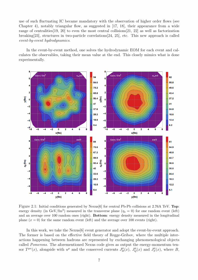
Figure 2.1: Initial conditions generated by Nexus[6] for central Pb-Pb collisions at 2.76A TeV. Top:energy density (in GeV/fm3) measured in the transverse plane (ηs = 0) for one random event (left)and an average over 100 random ones (right). Bottom: energy density measured in the longitudinalplane (x = 0) for the same random event (left) and the average over 100 events (right).

In this work, we take the Nexus[6] event generator and adopt the event-by-event approach.The former is based on the effective field theory of Regge-Gribov, where the multiple inter-actions happening between hadrons are represented by exchanging phenomenological objectscalled Pomerons. The aforementioned Nexus code gives as output the energy-momentum ten-sor T µν(x), alongside with uµ and the conserved currents JµB(x), JµQ(x) and JµS (x), where B,

7

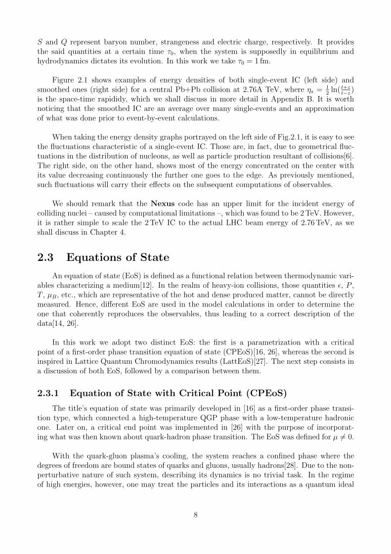
S and Q represent baryon number, strangeness and electric charge, respectively. It providesthe said quantities at a certain time τ0, when the system is supposedly in equilibrium andhydrodynamics dictates its evolution. In this work we take τ0 = 1 fm.

Figure 2.1 shows examples of energy densities of both single-event IC (left side) andsmoothed ones (right side) for a central Pb+Pb collision at 2.76A TeV, where ηs = 1

2ln( t+z

t−z )is the space-time rapididy, which we shall discuss in more detail in Appendix B. It is worthnoticing that the smoothed IC are an average over many single-events and an approximationof what was done prior to event-by-event calculations.

When taking the energy density graphs portrayed on the left side of Fig.2.1, it is easy to seethe fluctuations characteristic of a single-event IC. Those are, in fact, due to geometrical fluc-tuations in the distribution of nucleons, as well as particle production resultant of collisions[6].The right side, on the other hand, shows most of the energy concentrated on the center withits value decreasing continuously the further one goes to the edge. As previously mentioned,such fluctuations will carry their effects on the subsequent computations of observables.

We should remark that the Nexus code has an upper limit for the incident energy ofcolliding nuclei – caused by computational limitations –, which was found to be 2 TeV. However,it is rather simple to scale the 2 TeV IC to the actual LHC beam energy of 2.76 TeV, as weshall discuss in Chapter 4.

2.3 Equations of State

An equation of state (EoS) is defined as a functional relation between thermodynamic vari-ables characterizing a medium[12]. In the realm of heavy-ion collisions, those quantities ε, P ,T , µB, etc., which are representative of the hot and dense produced matter, cannot be directlymeasured. Hence, different EoS are used in the model calculations in order to determine theone that coherently reproduces the observables, thus leading to a correct description of thedata[14, 26].

In this work we adopt two distinct EoS: the first is a parametrization with a criticalpoint of a first-order phase transition equation of state (CPEoS)[16, 26], whereas the second isinspired in Lattice Quantum Chromodynamics results (LattEoS)[27]. The next step consists ina discussion of both EoS, followed by a comparison between them.

2.3.1 Equation of State with Critical Point (CPEoS)

The title’s equation of state was primarily developed in [16] as a first-order phase transi-tion type, which connected a high-temperature QGP phase with a low-temperature hadronicone. Later on, a critical end point was implemented in [26] with the purpose of incorporat-ing what was then known about quark-hadron phase transition. The EoS was defined for µ 6= 0.

With the quark-gluon plasma’s cooling, the system reaches a confined phase where thedegrees of freedom are bound states of quarks and gluons, usually hadrons[28]. Due to the non-perturbative nature of such system, describing its dynamics is no trivial task. In the regimeof high energies, however, one may treat the particles and its interactions as a quantum ideal

8

gas[16]. By virtue of the wave function’s symmetry properties, the former’s quantum state isfully characterized by the set of occupation numbers[29]:

{n1, n2, . . . , nj, . . . } ≡ {nj}, (2.13)

where nj represents the number of particles in orbital j. In the case of fermions, nj = 0 or1, while for bosons, nj could assume any value from 0 to N , with N as the total number ofparticles. The energy of said system is given by:

E =∑j

εjnj. (2.14)

Taking the context of the grand canonical ensemble, which represents a system in thermo-dynamic equilibrium, the grand partition function has the following expression:

ln Ξ = ±∑j

ln{1± exp(−β(εj − µ))} (2.15)

and the sum is over all single-particle quantum states. Additionally, the ± represents thestatistics of Fermi-Dirac (+) and Bose-Einstein (−) and β = 1/T . In the thermodynamic limit:

ln Ξ = ±g V

(2π)3

∫d3p ln{1± exp(−β(ε(p)− µ))}, (2.16)

where g is degeneracy factor, V the systems volume and ε(p) =√p2 +m2, with p as the

momentum of the particle and m as its mass. In the aforementioned limit, the pressure ofparticle j at temperature T with chemical potential µj is given by:

Pj(T, µj) = ± 1

βlimV→∞

1

Vln Ξ. (2.17)

Thus,

Pj(T, µj) =±gjβ(2π)3

∫d3p ln{1± exp(−β(εj(p)− µj))}. (2.18)

Integrating in spherical coordinates:

Pj(T, µj) =±gjβ(2π)3

4π

∫ ∞0

p2 ln(1± e−β(εj(p2)−µj))dp.

Integrating by parts shall yield the following result:

Pj(T, µj) =gj

6π2

∫ ∞0

p4√p2 +m2

j

1

eβ(εj−µj) ± 1dp, (2.19)

with mj as the j-th particle’s mass.

The total pressure of a hadron gas has the subsequent expression:

PHG(T, µ) =∑j

Pj(T, µj), (2.20)

which is a sum over all particle species and resonances. In order to get a practical applicationto hydrodynamics, we set all number densities save the baryonic one to be null everywhere[16].Hence, µj = BjµB, with B as the baryon number. The equation above becomes:

9

PHG(T, µB) =∑j

gj6π2

∫ ∞0

p4√p2 +m2

j

1

eβ(εj−BjµB) ± 1dp. (2.21)

The baryon number is defined as B = 13(q − q), where q and q represent the numbers of quark

and anti-quarks respectively. For mesons, B = 0 whereas for baryons −1 < B < 1. It is alsoimportant to remark that mesons are bosons while baryons are fermions. Knowing that, weshall rewrite PHG:

PHG(T, µB) =∑j

{fermions}

gj6π2

∫ ∞0

p4√p2 +m2

j

1

eβ(√p2+m2

j−BjµB) + 1dp

+∑j

{bosons}

gj6π2

∫ ∞0

p4√p2 +m2

j

1

eβ√p2+m2

j − 1dp. (2.22)

From the analysis of thermal models, it becomes clear that the ideal gas approach requires amodification to adjust the size of the system[16]. Since the volume to fit the particle abundancesis found to be small, one should then introduce the excluded-volume correction, represented bythe coupled equations below[16]:

PHG(T, µB) =∑j=1

P idj (T, µj), (2.23)

µj ≡ µj − υjPHG, (2.24)

where υj is the excluded volume of the j-th hadron species and P idj (T, µj) corresponds to the

pressure in expression (2.19). The remaining thermodynamic variables are calculated with therelations:

nB =

(∂PHG∂µB

)V,T

=∑j

(∂Pj∂µB

)=∑j

Bjnj, (2.25)

with nj as the j-th particle baryon number density. As for energy and entropy densities:

s =∂PHG∂T

,

ε = −PHG + Ts+ µnB.

In regard to the resonances included in the hadron gas, all meson and baryon massessmaller than 1.5 GeV and 2 GeV, respectively, are taken into consideration. Resonance widthsare not included[16]. We shall move on to the equation for the QGP phase.

10

Quantum Chromodynamics (QCD) is thought to possess two striking features: asymp-totic freedom and confinement. The first dictates that particle interactions weaken at shorterdistances. The second, on the other hand, states that quarks and gluons cannot be found asisolated objects. However, as energy and temperature increase, a phase transition may occurto a state where the degrees of freedom correspond to the color charged particles themselves[14]. Such stage is the aforementioned Quark-Gluon Plasma.

Taking the QCD properties cited above into consideration, the MIT Bag Model[30] assumesthat quarks and gluons are asymptotically free inside hadrons, which is a simple approach todescribe the latter’s structure. It proposes that strongly interacting particles consist of fieldsconfined to a finite region of space that possesses a constant positive potential energy per unitvolume, B [31]. One calls such region a bag. Boundary conditions ensure that fields vanishoutside it.

This MIT Bag description of a hadron as fields confined to a volume V could be extendedas means of computing an EoS for the QGP phase[16]. In that case, the QGP will be taken asan ideal quark-gluon gas restricted by V , with total energy given by[30]:

E = Er + BV⇒ ε = εr + B, (2.26)

where Er and εr are, respectively, the gas internal energy and energy density. Additionally, thepressure will take the form:

P = Pr − B. (2.27)

Combining the expression above with (2.21) will yield the following equation for QGPpressure:

PQGP =∑j

gj6π2

∫ ∞0

p4√p2 +m2

j

dp

eβ(√p2+m2

j−µj) ± 1− B. (2.28)

The sum is over gluons and up, down and strange quarks. One may write it more explicitly as:

PQGP =∑

{u,u,d,d,s,s}

gj6π2

∫ ∞0

p4√p2 +m2

j

dp

eβ(√p2+m2

j−BjµB) + 1

+gG6π2

∫ ∞0

p3

eβp − 1dp− B, (2.29)

where gj = 2× 3 and gG = 2× 8. Then, neglecting the masses of the up and down quarks,

PQGP =∑{u,u,d,d}

gj6π2

∫ ∞0

p3dp

eβ(p−BjµB) + 1+

gG6π2

∫ ∞0

p3

eβp − 1dp

+∑{s,s}

gj6π2

∫ ∞0

p4√p2 +m2

j

dp

eβ(√p2+m2

j−BjµB)− B. (2.30)

11

In this work we adopt the bag constant value as B = 380 MeV/fm3[16].

As the Quark-Gluon Plasma cools down, confinement wins over and, consequently, thedegrees of freedom correspond to the formed hadrons. The type of phase transition betweenQGP and HG varies with the value of µ[26, 32].

Let µ ∼ 0. Current QCD simulations with non-zero quark masses indicate the transitionas an analytical crossover[33]. Put differently, at a certain temperature interval, the thermody-namic variables rapidly change without any singularities.

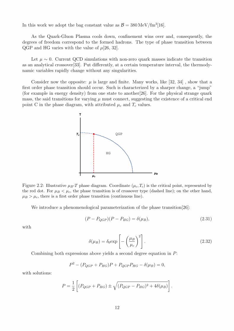
Consider now the opposite: µ is large and finite. Many works, like [32, 34] , show that afirst order phase transition should occur. Such is characterized by a sharper change, a “jump”(for example in energy density) from one state to another[26]. For the physical strange quarkmass, the said transitions for varying µ must connect, suggesting the existence of a critical endpoint C in the phase diagram, with attributed µc and Tc values.

HG

QGP

μcμB

Tc

T

Figure 2.2: Illustrative µB-T phase diagram. Coordinate (µc, Tc) is the critical point, represented bythe red dot. For µB < µc, the phase transition is of crossover type (dashed line); on the other hand,µB > µc, there is a first order phase transition (continuous line).

We introduce a phenomenological parameterization of the phase transition[26]:

(P − PQGP )(P − PHG) = δ(µB), (2.31)

with

δ(µB) = δ0exp

[−(µBµc

)2]. (2.32)

Combining both expressions above yields a second degree equation in P :

P 2 − (PQGP + PHG)P + PQGPPHG − δ(µB) = 0,

with solutions:

P =1

2

[(PQGP + PHG)±

√(PQGP − PHG)2 + 4δ(µB)

].

12

If µB � µc, δ(µB) should approach 0. In that case, the solutions above would be P = PQGP(positive sign) and P = PHG (negative sign). As previously mentioned, for large values ofµB, the phase transition should be of first order. Hence, PHG(T, µB) = PQGP (T, µB) whenboth states are in equilibrium. When considering this situation, it is possible to choose eithersolution. For all subsequent calculations, we take the one with positive sign. Thus, by defining:

λ ≡ 1

2

[1− (PQGP − PHG)√

(PQGP − PHG)2 + 4δ(µB)

], (2.33)

one can write the pressure in terms of λ:

P =1

2

[−(PQGP − PHG) + 2PQGP +

√(PQGP − PHG)2 + 4δ(µB)

]=

1

2

√(PQGP − PHG)2 + 4δ(µB)

[1− (PQGP − PHG)− 2PQGP√

(PQGP − PHG)2 + 4δ(µB)

]= λ

√(PQGP − PHG)2 + 4δ(µB) + PQGP .

Adding and subtracting 2δ(µB)√(PQGP−PHG)2+4δ(µB)

,

P = PQGP +2δ(µB)√

(PQGP − PHG)2 + 4δ(µB)+ λ√

(PQGPPHG)2 + 4δ(µB)

− 2δ(µB)√(PQGP − PHG)2 + 4δ(µB)

= PQGP +2δ(µB)√

(PQGP − PHG)2 + 4δ(µB)+λ[(PQGP − PHG)2 + 4δ(µB)]− 2δ(µB)√

(PQGP − PHG)2 + 4δ(µB).

By using (2.33) and simplifying, one arrives at the following result:

P = λPHG + (1− λ)PQGP +2δ(µB)√

(PQGP − PHG)2 + 4δ(µB). (2.34)

In order to compute nB, one must use the thermodynamic relation:

nB =

(∂P

∂µB

)T

=∂

∂µB(PHGλ) +

∂

∂µB(1− λ)PQGP

+∂

∂µB

[2δ(µB)√

(PQGP − PHG)2 + 4δ(µB)

]. (2.35)

We shall evaluate each term separately. Firstly:

∂

∂µB(PIλ) = λnI + PI

∂λ

∂µB,

where I could stand for either HG or QGP, and

13

∂λ

∂µB= −1

2

{(nQGP − nHG)

[(PQGP − PHG)2 + 4δ(µB)

]−1/2

− 1

2(PQGP − PHG)

[2(PQGP − PHG)(nQGP − nHG)

+ 4(−2)(µB/µ2c)δ(µB)

] [(PQGP − PHG)2 + 4δ(µB)

]−3/2 }.

Secondly, we take the derivative of the remaining term:

∂

∂µB

[2δ(µB)√

(PQGP − PHG)2 + 4δ(µB)

]= 2(−2)

(µBµ2c

)δ(µB)

[(PQGP − PHG)2 + 4δ(µB)

]−1/2

− δ(µB)

[2(PQGP − PHG)(nQGP − nHG)− 8

(µBµ2c

)δ(µB)

] [(PQGP − PHG)2 + 4δ(µB)

]−3/2.

Substituting the expressions above in (2.35) and simplifying shall result in:

nB = λnHG + (1− λ)nQGP −2(µB/µ

2c)δ(µB)√

(PQGP − PHG)2 + 4δ(µB). (2.36)

Knowing that s = ∂P∂T

, we can compute the entropy density:

s =∂

∂T(PHGλ) +

∂

∂T(1− λ)PQGP +

∂

∂T

[2δ(µB)√

(PQGP − PHG)2 + 4δ(µB)

](2.37)

We take each term’s derivative separately:

∂λ

∂T= −1

2

[(sQGP − sHG)√

(PQGP − PHG)2 + 4δ(µB)− (PQGP − PHG)(sQGP − sHG)

[(PQGP − PHG)2 + 4δ(µB)]3/2

]and

∂

∂T

[2δ(µB)√

(PQGP − PHG)2 + 4δ(µB)

]=

(−2)δ(µB)(PQGP − PHG)(sQGP − sHG)

[(PQGP − PHG)2 + 4δ(µB)]3/2.

By substituting in (2.37) and simplifying, we shall then have:

s = λsHG + (1− λ)sQGP . (2.38)

Finally, we use ε = −P + Ts+ µBnB to find the expression for energy density:

ε = λεHG + (1− λ)εQGP −2 [1 + (µB/µc)

2] δ(µB)√(PQGP − PHG)2 + 4δ(µB)

. (2.39)

CPEoS is now complete and can be used as input in the EoM of hydrodynamics.

14

2.3.2 Lattice QCD Equation of State (LattEoS)

Lattice simulations of QCD are able to depict the dynamics of strongly interacting matternon-perturbatively. Hence, a lattice QCD-based equation of state should be a fundamentalingredient in the evolution of heavy ion collisions, particularly of the Quark-Gluon Plasma.

EoS computations on the lattice at finite temperatures are performed using a fixed tem-poral extent Nτ and the temperature is varied by changing lattice spacing T = 1/(Nτa) [27].Therefore, hadron masses, which are dependent on temperature, also alter with lattice spac-ing (a). Since with decreasing T , a increases, the result shows a discrepancy between latticecalculations and predictions of the hadron resonance gas (HRG) model – in this case, there isno excluded volume correction. Other differences arise due to the quark masses used in latticeQCD being a factor of two larger than the physical ones [27].

HRG model is an useful tool for studying the high number of particles produced in heavyion collisions, up to a certain temperature limit. At the same time, lattice spacing for high Tdiminishes discretization errors, making lattice QCD calculations at such regime more accurate.The resulting EoS is an interpolation between hadron resonance gas at low T and lattice QCDat high T .

Energy and entropy density as well as pressure have their values computed by calculatingthe trace anomaly of the energy-momentum tensor, defined as Θ(T ) ≡ T µµ = ε − 3P (T ).Alongside with s = (ε + P )/T for nB = 0 (which is the case for the EoS at hand) ands = ∂P/∂T , one should have:

ε− 3P = Θ,

ε+ P = T∂P

∂T.

Subtracting one from the other:

Θ = T∂P

∂T− 4P.

Multiplying by T 5/T 5:

Θ = T 5 1

T 4

∂P

∂T+ T 5P (−4)

1

T 5

Θ = T 5∂(P/T 4)

∂T. (2.40)

Hence, the pressure difference at temperatures T and Tlow is expressed as the integral of thetrace anomaly:

P (T )

T 4− P (Tlow)

T 4low

=

∫ T

T low

dT ′

T ′5Θ(T ′). (2.41)

If one chooses the lower integration limit sufficiently small, P (Tlow) can be ignored due toexponential suppression. The remaining thermodynamic quantities, energy and entropy densityare computed using ε(T ) = Θ(T ) + 3P (T ) and s(T ) = (ε+ P )/T , respectively.

15

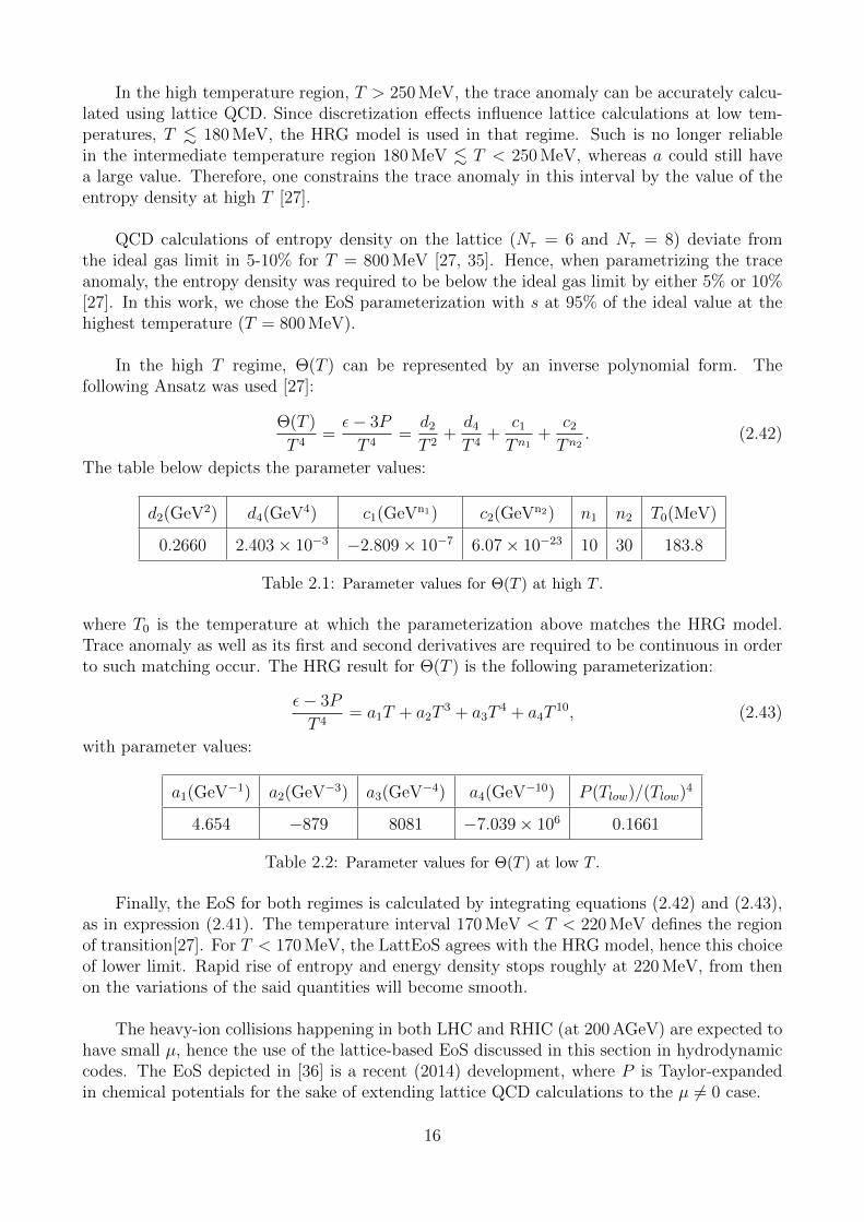
In the high temperature region, T > 250 MeV, the trace anomaly can be accurately calcu-lated using lattice QCD. Since discretization effects influence lattice calculations at low tem-peratures, T . 180 MeV, the HRG model is used in that regime. Such is no longer reliablein the intermediate temperature region 180 MeV . T < 250 MeV, whereas a could still havea large value. Therefore, one constrains the trace anomaly in this interval by the value of theentropy density at high T [27].

QCD calculations of entropy density on the lattice (Nτ = 6 and Nτ = 8) deviate fromthe ideal gas limit in 5-10% for T = 800 MeV [27, 35]. Hence, when parametrizing the traceanomaly, the entropy density was required to be below the ideal gas limit by either 5% or 10%[27]. In this work, we chose the EoS parameterization with s at 95% of the ideal value at thehighest temperature (T = 800 MeV).

In the high T regime, Θ(T ) can be represented by an inverse polynomial form. Thefollowing Ansatz was used [27]:

Θ(T )

T 4=ε− 3P

T 4=d2

T 2+d4

T 4+

c1

T n1+

c2

T n2. (2.42)

The table below depicts the parameter values:

d2(GeV2) d4(GeV4) c1(GeVn1) c2(GeVn2) n1 n2 T0(MeV)

0.2660 2.403× 10−3 −2.809× 10−7 6.07× 10−23 10 30 183.8

Table 2.1: Parameter values for Θ(T ) at high T .

where T0 is the temperature at which the parameterization above matches the HRG model.Trace anomaly as well as its first and second derivatives are required to be continuous in orderto such matching occur. The HRG result for Θ(T ) is the following parameterization:

ε− 3P

T 4= a1T + a2T

3 + a3T4 + a4T

10, (2.43)

with parameter values:

a1(GeV−1) a2(GeV−3) a3(GeV−4) a4(GeV−10) P (Tlow)/(Tlow)4

4.654 −879 8081 −7.039× 106 0.1661

Table 2.2: Parameter values for Θ(T ) at low T .

Finally, the EoS for both regimes is calculated by integrating equations (2.42) and (2.43),as in expression (2.41). The temperature interval 170 MeV < T < 220 MeV defines the regionof transition[27]. For T < 170 MeV, the LattEoS agrees with the HRG model, hence this choiceof lower limit. Rapid rise of entropy and energy density stops roughly at 220 MeV, from thenon the variations of the said quantities will become smooth.

The heavy-ion collisions happening in both LHC and RHIC (at 200 AGeV) are expected tohave small µ, hence the use of the lattice-based EoS discussed in this section in hydrodynamiccodes. The EoS depicted in [36] is a recent (2014) development, where P is Taylor-expandedin chemical potentials for the sake of extending lattice QCD calculations to the µ 6= 0 case.

16

2.3.3 Comparison between EoS

Having presented both EoS used in this work, we shall proceed on comparing them. Suchanalysis comprises a discussion on three stages of the hydrodynamic expansion of two collidingnuclei: Quark-Gluon Plasma, Hadron Gas and the phase transition between them.

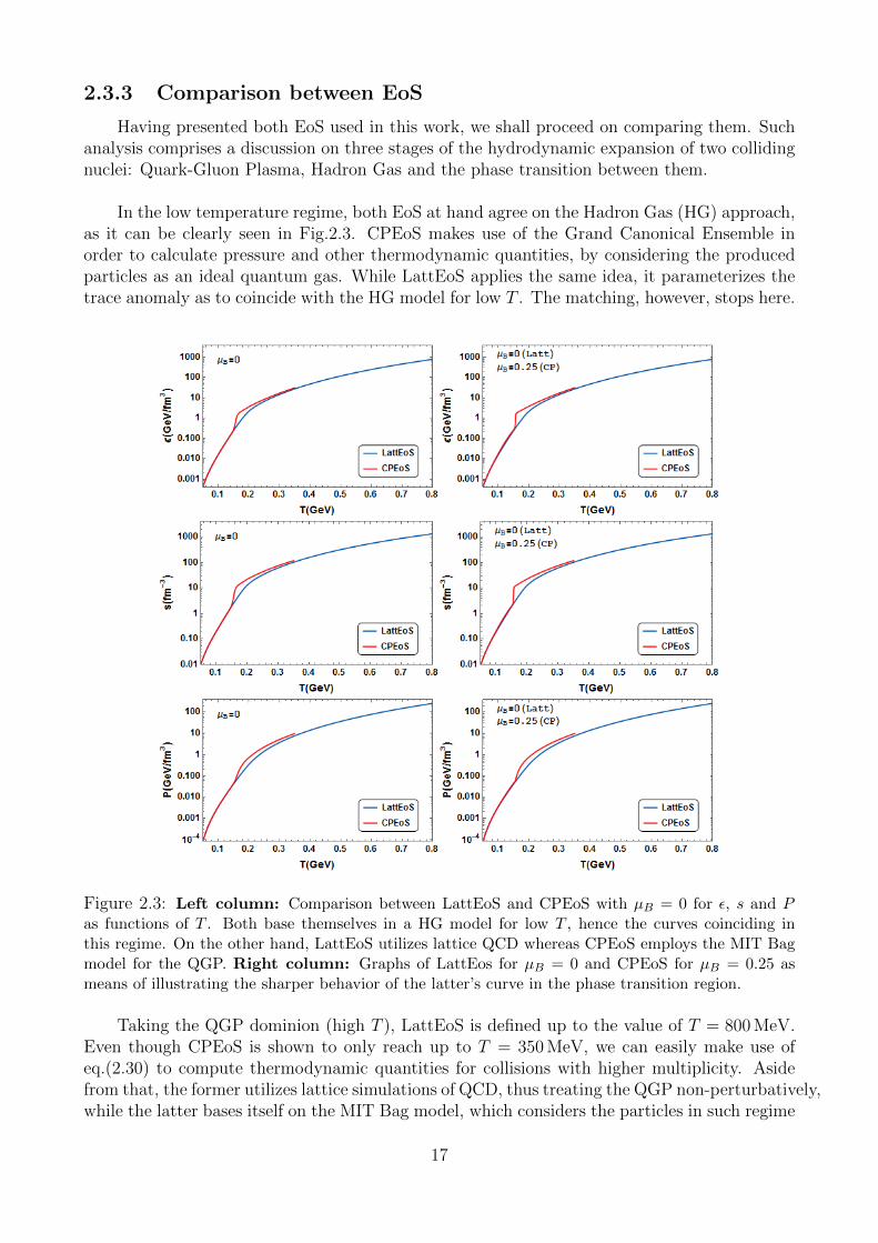
In the low temperature regime, both EoS at hand agree on the Hadron Gas (HG) approach,as it can be clearly seen in Fig.2.3. CPEoS makes use of the Grand Canonical Ensemble inorder to calculate pressure and other thermodynamic quantities, by considering the producedparticles as an ideal quantum gas. While LattEoS applies the same idea, it parameterizes thetrace anomaly as to coincide with the HG model for low T . The matching, however, stops here.

Figure 2.3: Left column: Comparison between LattEoS and CPEoS with µB = 0 for ε, s and Pas functions of T . Both base themselves in a HG model for low T , hence the curves coinciding inthis regime. On the other hand, LattEoS utilizes lattice QCD whereas CPEoS employs the MIT Bagmodel for the QGP. Right column: Graphs of LattEos for µB = 0 and CPEoS for µB = 0.25 asmeans of illustrating the sharper behavior of the latter’s curve in the phase transition region.

Taking the QGP dominion (high T ), LattEoS is defined up to the value of T = 800 MeV.Even though CPEoS is shown to only reach up to T = 350 MeV, we can easily make use ofeq.(2.30) to compute thermodynamic quantities for collisions with higher multiplicity. Asidefrom that, the former utilizes lattice simulations of QCD, thus treating the QGP non-perturbatively,while the latter bases itself on the MIT Bag model, which considers the particles in such regime

17

as an ideal quark-gluon gas with a bag constant.

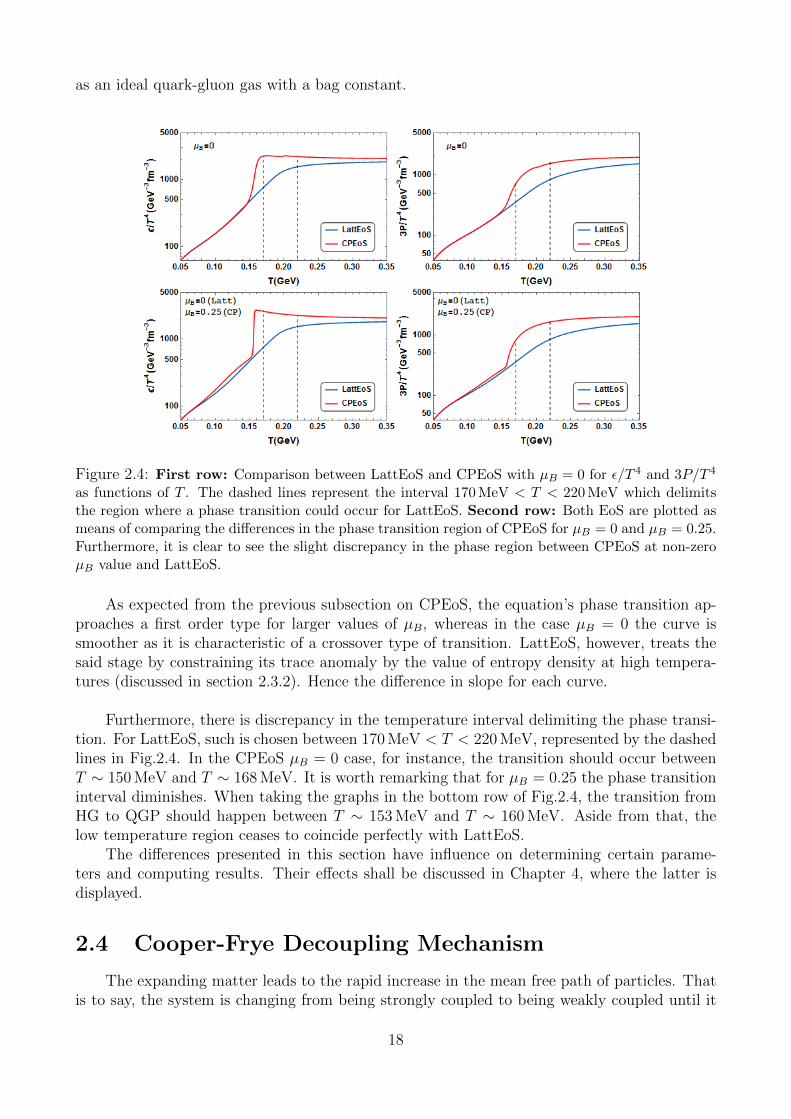
Figure 2.4: First row: Comparison between LattEoS and CPEoS with µB = 0 for ε/T 4 and 3P/T 4

as functions of T . The dashed lines represent the interval 170 MeV < T < 220 MeV which delimitsthe region where a phase transition could occur for LattEoS. Second row: Both EoS are plotted asmeans of comparing the differences in the phase transition region of CPEoS for µB = 0 and µB = 0.25.Furthermore, it is clear to see the slight discrepancy in the phase region between CPEoS at non-zeroµB value and LattEoS.

As expected from the previous subsection on CPEoS, the equation’s phase transition ap-proaches a first order type for larger values of µB, whereas in the case µB = 0 the curve issmoother as it is characteristic of a crossover type of transition. LattEoS, however, treats thesaid stage by constraining its trace anomaly by the value of entropy density at high tempera-tures (discussed in section 2.3.2). Hence the difference in slope for each curve.

Furthermore, there is discrepancy in the temperature interval delimiting the phase transi-tion. For LattEoS, such is chosen between 170 MeV < T < 220 MeV, represented by the dashedlines in Fig.2.4. In the CPEoS µB = 0 case, for instance, the transition should occur betweenT ∼ 150 MeV and T ∼ 168 MeV. It is worth remarking that for µB = 0.25 the phase transitioninterval diminishes. When taking the graphs in the bottom row of Fig.2.4, the transition fromHG to QGP should happen between T ∼ 153 MeV and T ∼ 160 MeV. Aside from that, thelow temperature region ceases to coincide perfectly with LattEoS.

The differences presented in this section have influence on determining certain parame-ters and computing results. Their effects shall be discussed in Chapter 4, where the latter isdisplayed.

2.4 Cooper-Frye Decoupling Mechanism

The expanding matter leads to the rapid increase in the mean free path of particles. Thatis to say, the system is changing from being strongly coupled to being weakly coupled until it

18

consists of substantially free streaming particles. Such stage in the evolution of matter is definedas thermal or kinetic freeze-out[14]. This work shall adopt the Cooper-Frye description[37] tomodel the said decoupling process. Other methods such as continuous emission and transportmodel will not be addressed.

The approach mentioned above assumes that the hadronic fluid suddenly stops interactingwhen the temperature falls to a decoupling value. Furthermore, it relies on the assumptionof the particle momentum distribution being unaffected by the system’s decoupling. In otherwords, the particle spectrum is evaluated on the freeze-out hypersurface σ characterized by:

Tfo = T (t, x, y, z), (2.44)

where Tfo is called freeze-out temperature. We shall address how these isotherms are deter-mined in Chapter 4.

In order to compute the momentum distribution of the particles crossing σ, one shall beginby portraying a many-body system as a collection of world lines. Let dσµ be the surface’snormal four-vector at some space-time point xµ and Dp = 2θ(p0)δ(p2−m2)d4p the four-volumein momentum space restricted to the mass-shell, centered on pµ. The net number of linestransiting across dσµ is, thus, given by:

dNW = fW (x, p)pµdσµDp, (2.45)

where fW (x, p) is the word line distribution function. Since σ is, in general, an arbitrary hyper-surface, dNW may not coincide with the net number of particles in said infinitesimal volumeof the phase-space at a certain time, dN [38]. In other words, when σ is space-like, its normalvector is time-like and dσµp

µ > 0, meaning that particles are leaving the surface. In such case,dNW = dN . However, if σ is time-like, one can have either dσµp

µ > 0 or dσµpµ < 0. In the

latter, particles are actually returning to the fluid, causing dNW 6= dN [39]. In this work, withfluctuating initial conditions, the number of returning particles is assumed to be negligible [40].

With dNW = dN , fW (x, p) should be the standard one-particle distribution function. Inaccordance to that, one has the following expression for the net number of particles crossing σat a certain time t, with given four-momentum between pµ and pµ + Dp:

dN = f(x, p)pµdσµDp, (2.46)

whose integral

N =

∫Dp

∫σ

f(x, p)pµdσµ (2.47)

counts the total number of emitted particles. One can also write it as the following:

N =

∫2θ(p0)δ(p2 −m2)d4p

∫σ

f(x, p)pµdσµ

=

∫2θ(p0)δ(p2

0 − ~p 2 −m2)d4p

∫σ

f(x, p)pµdσµ

Since E2 = ~p 2 +m2, N can be expressed as:

19

N =

∫2θ(p0)δ(p2

0 − E2)d4p

∫σ

f(x, p)pµdσµ.

Knowing that δ(x2 − a2) = 12|a|(δ(x+ a) + δ(x− a)):

N =

∫2θ(p0)

1

2E(δ(p0 + E) + δ(p0 − E))d4p

∫σ

f(x, p)pµdσµ,

with θ(p0) = 0, if p0 < 0 or θ(p0) = 1, if p0 > 0, one shall finally have:

N =

∫d3p

E

∫σ

f(x, p)pµdσµ. (2.48)

Alternately, (2.48) can give the particle distribution in momentum space:

EdN

d3p=

∫σ

f(x, p)pµdσµ, (2.49)

which is the said Cooper-Frye formula[37]. Due to the fluid being in local thermodynamicequilibrium as well as the assumption that there is no change in f(x, p) during the decouplingprocess, the latter can be expressed as:

f(x, p) =g

2π3

1

(e(pµuµ−µB)/T ± 1), (2.50)

where the positive sign indicates a Fermi-Dirac distribution, while the negative one, a Bose-Einstein distribution; g is the degeneracy factor associated to the particle to be considered.

20

Chapter 3

On NexSPheRIO

3.1 The SPH Method

In Section 2.1, we derived a non-linear set of differential equations to describe ideal rela-tivistic hydrodynamics. Due to their nature and the extremely complex medium caused by theIC fluctuations, it is no trivial task to solve those equations analytically, making numerical com-putation a desirable path to follow. In heavy-ion collisions, we take the hydrodynamic approachin order to infer information on its two main ingredients, the IC and EoS, from comparisonswith experimental data. In this work, we adopt the Smoothed-particle Hydrodynamics (SPH)computational method, as introduced in [41] and [42] in order to study astrophysical problems.The aforementioned can lead to a very precise solution of the hydrodynamic equations[43].

The SPH approach allows the study of system configurations with any geometry, as well asthe possibility of smoothing out unwanted local degrees of freedom. It is, therefore, a perfectfit to the variational formalism[7]. The basic idea of this method is to introduce a set of“particles” characterized by their Lagrangian coordinates {~ri}, which move with the fluid. Inorder to achieve that, we shall begin by considering the physical extensive quantity A, withcorresponding density distribution a(~r, t). We can write the latter as:

a(~r, t) =

∫a(~r ′, t)δ(~r − ~r ′)d3~r ′. (3.1)

In a first approximation, one should substitute δ(~r−~r ′) by a kernel function W , with withfinite support h and properties:

∫W (~r − ~r ′;h)d3~r ′ = 1, (3.2a)

limh→0

W (~r − ~r ′;h) = δ(~r − ~r ′), (3.2b)

which allows for expressing a(~r, t) as:

a(~r, t)→ a(~r, t) =

∫a(~r ′, t)W (~r − ~r ′;h)d3~r ′. (3.3)

The density a(~r, t) is a smoothed a(~r, t). W introduces a short-wavelength cut-off filter in theFourier representation of a(~r, t)[7]. For a practical application, one may reduce the degrees offreedom, by replacing the integral in (3.3) with a sum over a finite and discrete set of points,{~ri, i = 1, . . . , N}[16]:

21

a(~r, t)→ aSPH =N∑i

AiW (~r − ~ri;h), (3.4)

with weights Ai. Summing it all up:

a(~r, t)→ aSPH =N∑i

AiW (~r − ~ri;h). (3.5)

The latter is an ansatz which approximates a(~r, t) as a sum of finite dynamic “particles” withcoordinates ~ri, carrying the quantity Ai. Due to property 3.2a,∫

aSPH(~r, t)d3~r =N∑i

Ai,

with

Atot =N∑i

Ai

as the total amount of A in the system.

Since we deal with more than one extensive physical quantity in hydrodynamics, we choosea conserved quantity as the reference density, ρ, when applying the aforementioned method.The representation of ρ in the SPH form is

ρSPH(~r, t) =N∑i

%iW (~r − ~ri(t);h), (3.6)

where ~ri = ~ri(t) is the trajectory of the i-th “SPH particle and the weights {%i} are constantin time. In that case, the time derivative of ρSPH ,

∂

∂tρSPH(~r, t) =

N∑i

∂

∂t

(%iW (~r − ~ri(t);h)

),

takes the value

∂

∂tρSPH(~r, t) =

N∑i

%id

dtW (~r − ~ri(t);h)

= −N∑i

%id~ri(t)

dt∇ ·W (~r − ~ri(t);h).

Since d~ri(t)dt

= ~vi(t), the expression above becomes:

22

∂

∂tρSPH(~r, t) = −

N∑i

%i~vi(t)∇ ·W (~r − ~ri(t);h)

= −∇ ·N∑i

%i~vi(t)W (~r − ~ri(t);h)

= −∇ ·~jSPH(~r, t),

where

~jSPH(~r, t) =N∑i

%i~vi(t)W (~r − ~ri(t);h) (3.7)

is the SPH representation of ρ’s current density, ~j = ρ~v. Therefore, ρSPH satisfies the continuityequation:

∂

∂tρSPH +∇ ·~jSPH = 0, (3.8)

as expected.

It is rather simple to calculate other extensive quantities, such as A. Taking a as its density,then the amount of A carried by particle i for the unit reference ρ is:

Ai = %i

(a

ρ

)i

, (3.9)

so that the density distribution a(~r, t) becomes:

a(~r, t)→ aSPH(~r, t) =N∑i

(a

ρ

)i

%iW (~r − ~ri(t);h). (3.10)

Physically speaking, we are replacing a continuous fluid by a set of the so called “SPH par-ticles”. Moreover, we take the associated coordinates {~ri(t)} as variational degrees of freedom.Their equations of motion are thus obtained by minimizing the action for the hydrodynamicsystem.

Since we are interested in relativistic hydrodynamics, it is highly convenient to extend thevariational procedure to a general coordinate system, as in Appendix C. Hence the action fora relativistic fluid motion (from (C.9)):

I = −∫d4x√−gε, (3.11)

with constraints for conserved entropy (C.10) and baryon (C.11) densities:

(suµ);µ =1√−g

∂µ(√−gsuµ

)= 0, (3.12)

(nuµ);µ =1√−g

∂µ(√−gnuµ

)= 0. (3.13)

23

Let s∗ and n∗ be the entropy and baryon densities in a space-fixed frame. From expression(3.6), we may parameterize

√−gsγ = s∗ → s∗SPH =

∑i

νiW (~r − ~ri(τ)), (3.14)

√−gnγ = n∗ → n∗SPH =

∑i

βiW (~r − ~ri(τ)), (3.15)

Since ∫d3~rW (~r − ~ri) = 1, (3.16)

the total entropy and baryon number are

S =

∫d3~r√−gsγ =

∑i

νi, (3.17)

B =

∫d3~r√−gnγ =

∑i

βi. (3.18)

Analogously to (3.6), νi and βi are, respectively, the amount of entropy and baryon numbercarried by the i-th particle.

Since it is expected that most of the energy content is of non-baryonic nature (mostlypions), particularly in mid-rapidity regions (definition on Chapter 4), n is not suitable to beused as the reference density (ρ) in SPH representation[8]. Instead, the role falls on s, whichdoes not vanish in the region of interest. We have also stated in Appendix B that τ is a moreconvenient coordinate to employ in the study of heavy-ion collisions, hence ~ri = ~ri(τ). In ageneralized coordinate system, we use the notation τ = x0 and γ = u0. The latter’s generalizedexpression can be computed using

uµuµ = 1,

gµνuνuµ = 1.

We take the metric tensor as

(gµν) =

(g00 00 −g

)(3.19)

whose time-like coordinate is orthogonal to the space-like ones in order to unambiguously definethe conserved quantity s[16]. Also, −g is the 3× 3 space part of gµν . In this case,

gµνuνuµ = g00u

0u0 − gijuiuj = 1.

Since ui = γvi = u0vi,

g00u0u0 − gijvivju0u0 = 1

u20

(g00 − gijvivj

)= 1,

24

which yields

γ =1√

g00 − ~v Tg~v. (3.20)

We shall proceed on writing the action (3.11) in the SPH representation, by making use of(3.10) and (3.14):

ISPH = −∫dτ

∫d3~r∑i

νi

( √−gε√−gsγ

)i

W (~r − ~ri(τ)) (3.21)

= −∫dτ∑i

νi

(ε

sγ

)i

. (3.22)

Before moving on to the next step, we should define the specific volume Vi of S associated withparticle i,

Vi ≡νisi, (3.23)

and substitute it in ISPH :

ISPH = −∫dτ∑i

(εV

γ

)i

= −∫dτ∑i

(E

γ

)i

, (3.24)

with εiVi = Ei.

After minimizing the action above, one gets the following equation of motion[8]:

d~πidτ

= −∑j

νiνj

[Pi√−gγ2

i s2i

+Pj√−gγ2

j s2j

]∇iWij

−(∇ig00 − ~vi

Tg~vi) γiνi

2

(ε+ P

s

)i

+νiPiγisi

(1√−g∇i

√−g), (3.25)

with

~πi = γiνi

(P + ε

s

)i

g~vi. (3.26)

From Appendix B, we gather a rather convenient set of variables for heavy-ion collisions,the proper time, space-time rapidity and cartesian coordinates x and y:

τ =√t2 − z2, (3.27)

ηs =1

2ln

(t+ z

t− z

), (3.28)

~rT =

(xy

), (3.29)

25

respectively. Furthermore,

t = τ cosh(ηs)⇒ dt = cosh(ηs)dτ + τ sinh(ηs)dηs,

z = τ sinh(ηs)⇒ dz = sinh(ηs)dτ + τ cosh(ηs)dηs.

⇒ dt2 − dz2 = dτ 2 − τ 2dη2s

Since gµνdxµdxν = ηµνdξ

µdξν , with ξµ being coordinates in Minkowski space,

gµνdxµdxν = dt2 − dx2 − dy2 − dz2 = dτ 2 − dx2 − dy2 − τ 2dη2

s .

From the metric tensor depicted in (3.19),

g00 = 1, (3.30)

g =

1 0 00 1 00 0 τ 2

, (3.31)

√−g = τ. (3.32)

The parametrization (3.14) will thus become

τγisi = s∗i =∑j

νjW (qij),

where

qij =√

(xi − xj)2 + (yi − yj)2 + τ 2((ηs)i − (ηs)j)2.

Finally, the SPH equation of motion takes the form

d~πidτ≡ d

dτ

(~πTπηs

)i

= −1

τ

∑j

νiνj

[Piγis2

i

+Pjγjs2

j

]∇iWij, (3.33)

with

~πT = γν

(P + ε

s

)~vT , (3.34)

πηs = γν

(P + ε

s

)τvηs , (3.35)

where ~vT = d~rTdτ

and vηs = dηsdτ

. Since

~v Tg~v =(vx vy vηs

)1 0 00 1 00 0 τ

vxvyvηs

= ~v 2T + τ 2v2

ηs ,

the Lorentz factor (3.20) becomes

γ =1√

1− ~v 2T − τ 2v2

ηs

. (3.36)

26

The ordinary equations of motion presented above yield the velocities and positions of theSPH particles as a function of the expansion time, τ . They allow for computing the evolutionof all thermodynamic quantities, by taking also the equation of state and the parameterizationof the conserved quantity, s∗, alongside with its current, j∗ = ~vs∗.

3.2 Decoupling in SPH

Having derived the fluid’s equations of motion in the SPH formalism, it becomes clear thatsuch method should also be extended to the Cooper-Frye formula defined in Chapter 2,

EdN

d3p=

∫σ

dσµpµf (uµp

µ, T, µB) .

In order to compute the momentum distribution of SPH particles crossing the surface σ,we shall begin by approximating the expression above to a sum over all given particles in thesystem

EdN

d3p=∑j

(∆σnµ)j pµf (pµ(uµ)j, Tfo, (µB)j) , (3.37)

where ∆σj is a hypersurface element, (nµ)j its normal vector and

f (pµ(uµ)j, Tfo, (µB)j) =gj

2π3

[e(pµ(uµ)j−(µB)j)/Tfo ± 1

]−1. (3.38)

As (3.37) and (3.38) make explicit, the quantities with index j are inherent to the j-th particlewhen it is localized at σ, which in turn is defined by the isotherm Tfo.

Aside from ∆σj, all other quantities present in the expressions above can be computedrather directly from previously mentioned formulas by a method to be discussed in Chapter4. Therefore, it becomes necessary to write ∆σj in terms of more convenient quantities. Take,for instance, a particle j in its proper frame (PF ). In that case, pµ → p0, which implies thatpµ(nµ∆σ)j → p0(n0∆σ)j, when the particle reaches σ. Furthermore, (n0∆σ)j can be identifiedas (∆σ0)PFj , the proper hypersurface element.

Having established (∆σ0)PFj , it is worth recalling from its definition, that it possesses onlythe time component. Henceforth, ∣∣(∆σ0)PFj

∣∣ = Vj, (3.39)

where Vj is the 3-dimensional volume of the j-th particle in its proper frame. We thus proceedon recovering (∆σµ)j through a Lorentz transformation,

(∆σµ)j =[Λ0

µ(∆σ0)PF]j

=[(γ,−γvi)(∆σ0)PF

]j

=[uµ(∆σ0)PF

]j,

where we used the set of equations (2.5). Contracting with uµ on both sides, yield

(∆σ0)PFj = (uµ)j(∆σµ)j. (3.40)

Then,

27

Vj = |(uµ)j(∆σµ)j| = |(uµnµ)j|∆σj,

⇒ (∆σ)j =Vj

|(uµnµ)j|. (3.41)

Rewriting (3.37),

EdN

d3p=∑j

νj(nµ)jpµ

sj |(uµnµ)j|f (pµ(uµ)j, Tfo, (µB)j) , (3.42)

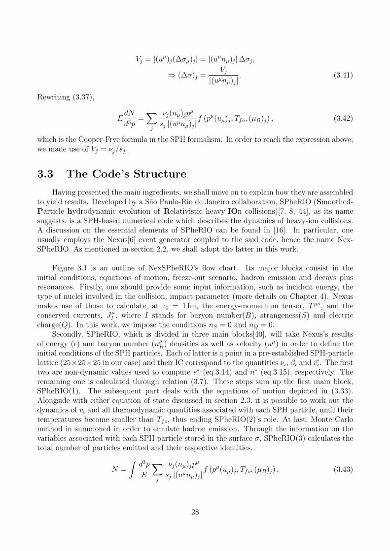
which is the Cooper-Frye formula in the SPH formalism. In order to reach the expression above,we made use of Vj = νj/sj.

3.3 The Code’s Structure

Having presented the main ingredients, we shall move on to explain how they are assembledto yield results. Developed by a Sao Paulo-Rio de Janeiro collaboration, SPheRIO (Smoothed-Particle hydrodynamic evolution of Relativistic heavy-IOn collisions)[7, 8, 44], as its namesuggests, is a SPH-based numerical code which describes the dynamics of heavy-ion collisions.A discussion on the essential elements of SPheRIO can be found in [16]. In particular, oneusually employs the Nexus[6] event generator coupled to the said code, hence the name Nex-SPheRIO. As mentioned in section 2.2, we shall adopt the latter in this work.

Figure 3.1 is an outline of NexSPheRIO’s flow chart. Its major blocks consist in theinitial conditions, equations of motion, freeze-out scenario, hadron emission and decays plusresonances. Firstly, one should provide some input information, such as incident energy, thetype of nuclei involved in the collision, impact parameter (more details on Chapter 4). Nexusmakes use of those to calculate, at τ0 = 1 fm, the energy-momentum tensor, T µν , and theconserved currents, JµI , where I stands for baryon number(B), strangeness(S) and electriccharge(Q). In this work, we impose the conditions nS = 0 and nQ = 0.

Secondly, SPheRIO, which is divided in three main blocks[40], will take Nexus’s resultsof energy (ε) and baryon number (nµB) densities as well as velocity (uµ) in order to define theinitial conditions of the SPH particles. Each of latter is a point in a pre-established SPH-particlelattice (25×25×25 in our case) and their IC correspond to the quantities νi, βi and ~vi. The firsttwo are non-dynamic values used to compute s∗ (eq.3.14) and n∗ (eq.3.15), respectively. Theremaining one is calculated through relation (3.7). These steps sum up the first main block,SPheRIO(1). The subsequent part deals with the equations of motion depicted in (3.33).Alongside with either equation of state discussed in section 2.3, it is possible to work out thedynamics of vi and all thermodynamic quantities associated with each SPH particle, until theirtemperatures become smaller than Tfo, thus ending SPheRIO(2)’s role. At last, Monte Carlomethod in summoned in order to emulate hadron emission. Through the information on thevariables associated with each SPH particle stored in the surface σ, SPheRIO(3) calculates thetotal number of particles emitted and their respective identities,

N =

∫d3p

E

∑j

νj(nµ)jpµ

sj |(uµnµ)j|f (pµ(uµ)j, Tfo, (µB)j) , (3.43)

28

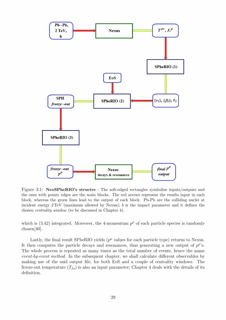
Figure 3.1: NexSPheRIO’s structre - The soft-edged rectangles symbolize inputs/outputs andthe ones with pointy edges are the main blocks. The red arrows represent the results input in eachblock, whereas the green lines lead to the output of each block. Pb-Pb are the colliding nuclei atincident energy 2 TeV (maximum allowed by Nexus); b is the impact parameter and it defines thechosen centrality window (to be discussed in Chapter 4).

which is (3.42) integrated. Moreover, the 4-momentum pµ of each particle species is randomlychosen[40].

Lastly, the final result SPheRIO yields (pµ values for each particle type) returns to Nexus.It then computes the particle decays and resonances, thus generating a new output of pµ’s.The whole process is repeated as many times as the total number of events, hence the nameevent-by-event method. In the subsequent chapter, we shall calculate different observables bymaking use of the said output file, for both EoS and a couple of centrality windows. Thefreeze-out temperature (Tfo) is also an input parameter; Chapter 4 deals with the details of itsdefinition.

29

Chapter 4

Results

4.1 Centrality Classes

In ultra-relativistic heavy-ion collisions, the energy involved is high enough to createparticle-antiparticle pairs. Therefore, the energy binding nucleons inside nuclei as well as thatof excited nuclear states may be ignored. As a result, only the spatial distribution of nucleonsand their cross section value have relevance to the collision outcome. Those are responsible forthe fluctuations in the initial energy density distribution observed and discussed in section 2.2.Considering that, we make use of simple geometric concepts (to be defined below) in order tostudy the initial moments of the colliding nuclei.

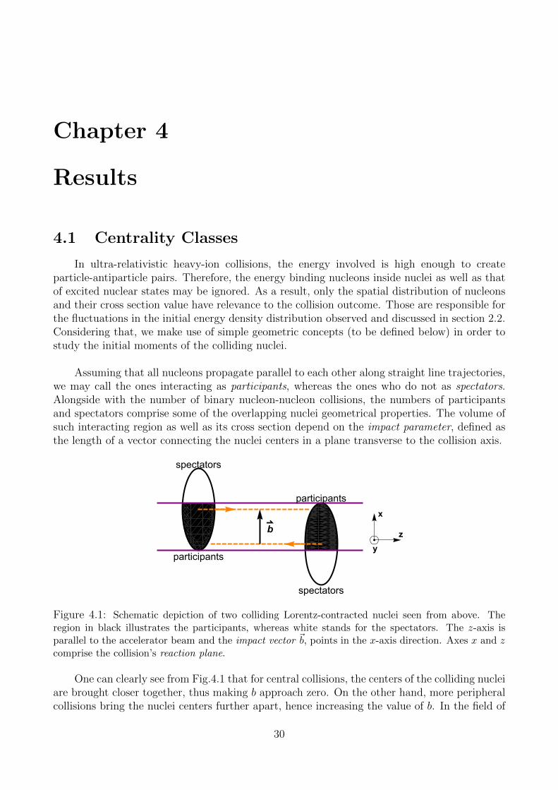
Assuming that all nucleons propagate parallel to each other along straight line trajectories,we may call the ones interacting as participants, whereas the ones who do not as spectators.Alongside with the number of binary nucleon-nucleon collisions, the numbers of participantsand spectators comprise some of the overlapping nuclei geometrical properties. The volume ofsuch interacting region as well as its cross section depend on the impact parameter, defined asthe length of a vector connecting the nuclei centers in a plane transverse to the collision axis.

b

spectators

participants

participants

spectators

x

z

y

Figure 4.1: Schematic depiction of two colliding Lorentz-contracted nuclei seen from above. Theregion in black illustrates the participants, whereas white stands for the spectators. The z-axis isparallel to the accelerator beam and the impact vector ~b, points in the x-axis direction. Axes x and zcomprise the collision’s reaction plane.

One can clearly see from Fig.4.1 that for central collisions, the centers of the colliding nucleiare brought closer together, thus making b approach zero. On the other hand, more peripheralcollisions bring the nuclei centers further apart, hence increasing the value of b. In the field of

30

heavy-ion collisions, it is customary to introduce a quantitative measure called centrality, whichis directly related to the impact parameter. The former is usually expressed as a percentage ofthe total nuclear interaction cross section σnuclcross [45]. In a nucleus-nucleus collision with impactparameter b, the centrality percentile c takes the form

c =

∫ b0dσcross/db

′db′∫∞0dσcross/db′db′

=1

σnuclcross

∫ b

0

dσcrossdb′

db′, (4.1)

where dσcross/db′ is the impact parameter distribution. The equation above may be simplified

by replacing the cross section using the number of events, N :

c ≈ 1

N

∫ b

0

dN

db′db′. (4.2)

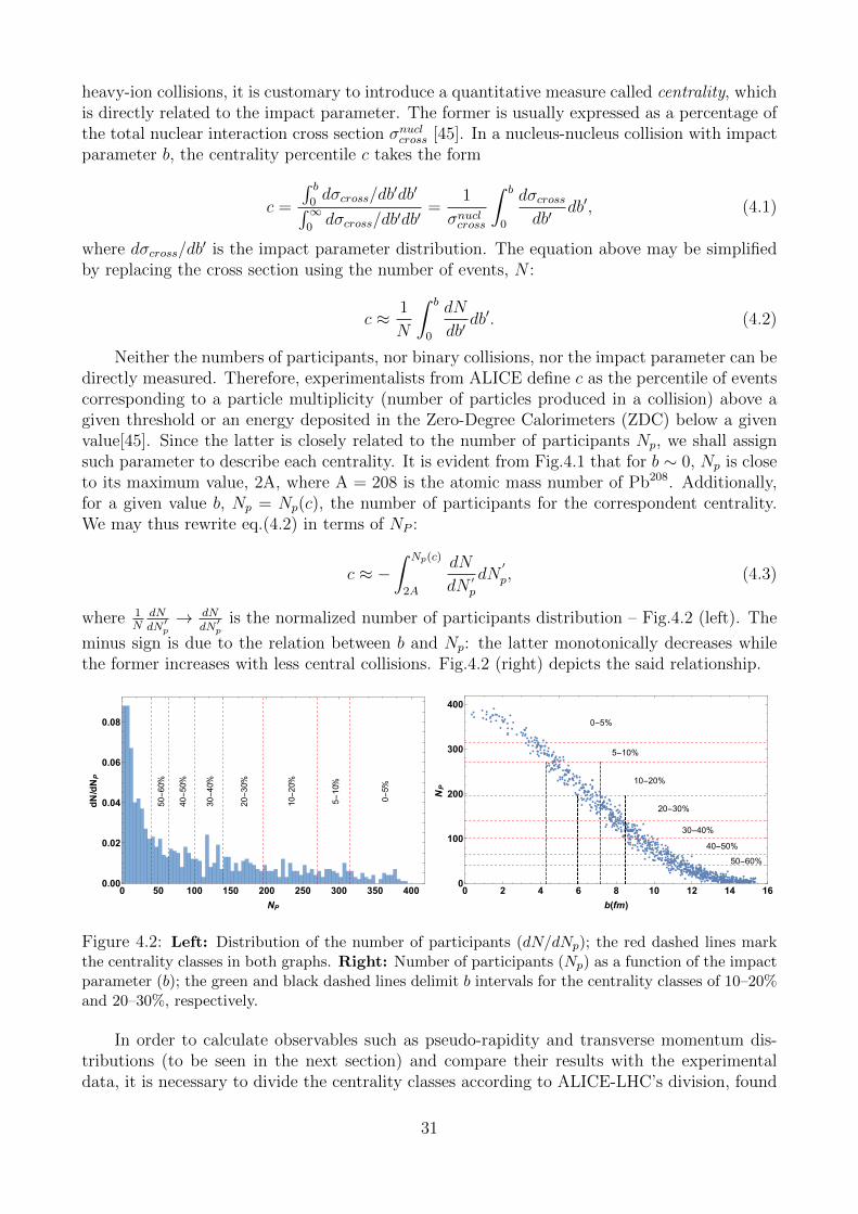
Neither the numbers of participants, nor binary collisions, nor the impact parameter can bedirectly measured. Therefore, experimentalists from ALICE define c as the percentile of eventscorresponding to a particle multiplicity (number of particles produced in a collision) above agiven threshold or an energy deposited in the Zero-Degree Calorimeters (ZDC) below a givenvalue[45]. Since the latter is closely related to the number of participants Np, we shall assignsuch parameter to describe each centrality. It is evident from Fig.4.1 that for b ∼ 0, Np is closeto its maximum value, 2A, where A = 208 is the atomic mass number of Pb208. Additionally,for a given value b, Np = Np(c), the number of participants for the correspondent centrality.We may thus rewrite eq.(4.2) in terms of NP :

c ≈ −∫ Np(c)

2A

dN

dN ′pdN

′

p, (4.3)

where 1N

dNdN ′p→ dN

dN ′pis the normalized number of participants distribution – Fig.4.2 (left). The

minus sign is due to the relation between b and Np: the latter monotonically decreases whilethe former increases with less central collisions. Fig.4.2 (right) depicts the said relationship.

0-5%

5-10%

10-20

%

20-30

%

30-40

%

40-50

%

50-60

%

0 50 100 150 200 250 300 350 4000.00

0.02

0.04

0.06

0.08

NP

dN/dNP

0-5%

5-10%

10-20%

20-30%

30-40%

40-50%

50-60%

0 2 4 6 8 10 12 14 160

100

200

300

400

b(fm)

NP

Figure 4.2: Left: Distribution of the number of participants (dN/dNp); the red dashed lines markthe centrality classes in both graphs. Right: Number of participants (Np) as a function of the impactparameter (b); the green and black dashed lines delimit b intervals for the centrality classes of 10–20%and 20–30%, respectively.

In order to calculate observables such as pseudo-rapidity and transverse momentum dis-tributions (to be seen in the next section) and compare their results with the experimentaldata, it is necessary to divide the centrality classes according to ALICE-LHC’s division, found

31

in [45, 46, 47]. Firstly, we employed the Nexus code to generate 1000 events with impact pa-rameter values spanning from b = 0 to b > 2RPb, the latter being the nuclear radius of lead.The distribution of the number of participants was then computed: we counted the number ofevents for given intervals of Np (Fig.4.2 left). From expression (4.3), it is possible to determinethe value of Np for each centrality class: taking 0–5%, for instance, one counts 5% of the eventswith higher multiplicity and checks the corresponding number of participants, thus obtainingNp(5%) ∼ 315. For the next centrality class, 5–10%, one repeats the aforementioned procedureand excludes the previous window (0–5%), which gives 270 . NP . 315. Those steps arerepeated for each centrality class.

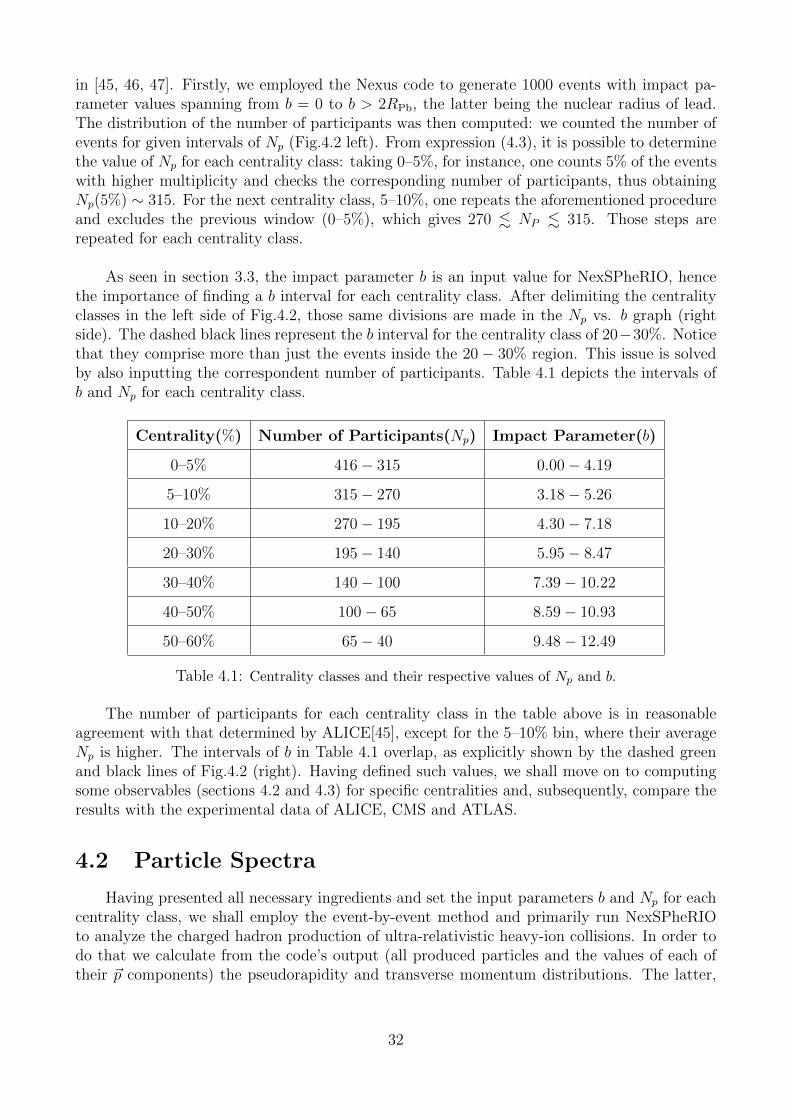
As seen in section 3.3, the impact parameter b is an input value for NexSPheRIO, hencethe importance of finding a b interval for each centrality class. After delimiting the centralityclasses in the left side of Fig.4.2, those same divisions are made in the Np vs. b graph (rightside). The dashed black lines represent the b interval for the centrality class of 20−30%. Noticethat they comprise more than just the events inside the 20− 30% region. This issue is solvedby also inputting the correspondent number of participants. Table 4.1 depicts the intervals ofb and Np for each centrality class.

Centrality(%) Number of Participants(Np) Impact Parameter(b)

0–5% 416− 315 0.00− 4.19

5–10% 315− 270 3.18− 5.26

10–20% 270− 195 4.30− 7.18

20–30% 195− 140 5.95− 8.47

30–40% 140− 100 7.39− 10.22

40–50% 100− 65 8.59− 10.93

50–60% 65− 40 9.48− 12.49

Table 4.1: Centrality classes and their respective values of Np and b.

The number of participants for each centrality class in the table above is in reasonableagreement with that determined by ALICE[45], except for the 5–10% bin, where their averageNp is higher. The intervals of b in Table 4.1 overlap, as explicitly shown by the dashed greenand black lines of Fig.4.2 (right). Having defined such values, we shall move on to computingsome observables (sections 4.2 and 4.3) for specific centralities and, subsequently, compare theresults with the experimental data of ALICE, CMS and ATLAS.

4.2 Particle Spectra

Having presented all necessary ingredients and set the input parameters b and Np for eachcentrality class, we shall employ the event-by-event method and primarily run NexSPheRIOto analyze the charged hadron production of ultra-relativistic heavy-ion collisions. In order todo that we calculate from the code’s output (all produced particles and the values of each oftheir ~p components) the pseudorapidity and transverse momentum distributions. The latter,

32

as its name suggests, is the particle 3-momentum component in the x-y (transverse) plane,designated by pT . The pseudorapidity variable, η, is defined as the following:

η ≡ 1

2ln

[|~p|+ pL|~p| − pL

]= − ln

(tan

θ

2

), (4.4)

where pL = pz is the 3-momentum longitudinal component and θ is the polar angle betweenthe charged particle direction and the beam axis.

Subsections 4.2.1 and 4.2.2 discuss the aforementioned distributions for the centralityclasses of 0–5% , 5–10%, 10–20% and 20–30% as well as both equations of state describedin Chapter 2. The results are then compared with ALICE data from [46, 47].

4.2.1 Pseudorapidity Distribution

One way of analyzing particle production in heavy-ion collisions is by computing the pseu-dorapidity spectrum, as previously mentioned. Since the latter does not require particle iden-tification, it presents itself as a viable candidate to compute the Nch distribution.

LHC produced Pb-Pb collisions at a center-of-mass energy per nucleon pair of√sNN =

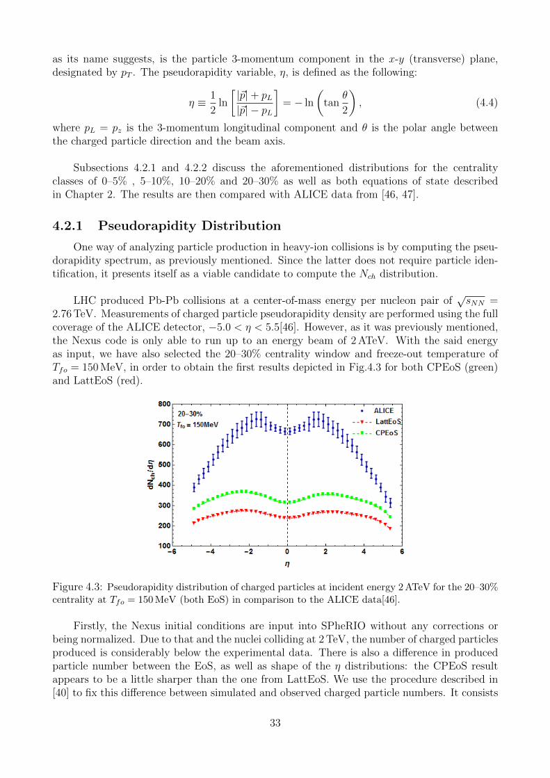
2.76 TeV. Measurements of charged particle pseudorapidity density are performed using the fullcoverage of the ALICE detector, −5.0 < η < 5.5[46]. However, as it was previously mentioned,the Nexus code is only able to run up to an energy beam of 2 ATeV. With the said energyas input, we have also selected the 20–30% centrality window and freeze-out temperature ofTfo = 150 MeV, in order to obtain the first results depicted in Fig.4.3 for both CPEoS (green)and LattEoS (red).

Figure 4.3: Pseudorapidity distribution of charged particles at incident energy 2 ATeV for the 20–30%centrality at Tfo = 150 MeV (both EoS) in comparison to the ALICE data[46].

Firstly, the Nexus initial conditions are input into SPheRIO without any corrections orbeing normalized. Due to that and the nuclei colliding at 2 TeV, the number of charged particlesproduced is considerably below the experimental data. There is also a difference in producedparticle number between the EoS, as well as shape of the η distributions: the CPEoS resultappears to be a little sharper than the one from LattEoS. We use the procedure described in[40] to fix this difference between simulated and observed charged particle numbers. It consists

33

in introducing a function dependent on ηs (spacetime rapidity) whose objective is to correct theinitial energy density (ε0) generated by Nexus along the longitudinal axis. In order to relate ε0with the pseudorapidity distribution of particles, we shall approximate

η =1

2ln

[|~p|+ pz|~p| − pz

]' ηs =

1

2ln

[t+ z

t− z

], (4.5)

which holds true at LHC energies. Such correction should preserve the fluctuations character-istic of an event initial energy density distribution.

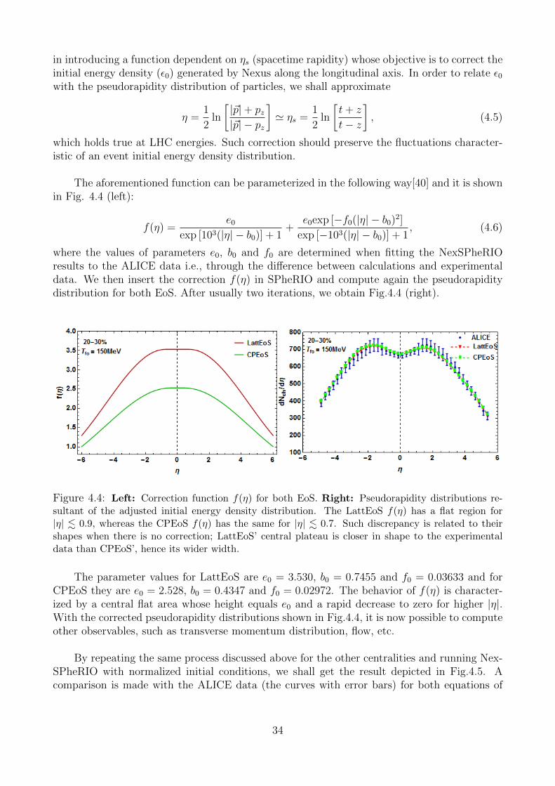
The aforementioned function can be parameterized in the following way[40] and it is shownin Fig. 4.4 (left):

f(η) =e0

exp [103(|η| − b0)] + 1+

e0exp [−f0(|η| − b0)2]

exp [−103(|η| − b0)] + 1, (4.6)

where the values of parameters e0, b0 and f0 are determined when fitting the NexSPheRIOresults to the ALICE data i.e., through the difference between calculations and experimentaldata. We then insert the correction f(η) in SPheRIO and compute again the pseudorapiditydistribution for both EoS. After usually two iterations, we obtain Fig.4.4 (right).

Figure 4.4: Left: Correction function f(η) for both EoS. Right: Pseudorapidity distributions re-sultant of the adjusted initial energy density distribution. The LattEoS f(η) has a flat region for|η| . 0.9, whereas the CPEoS f(η) has the same for |η| . 0.7. Such discrepancy is related to theirshapes when there is no correction; LattEoS’ central plateau is closer in shape to the experimentaldata than CPEoS’, hence its wider width.

The parameter values for LattEoS are e0 = 3.530, b0 = 0.7455 and f0 = 0.03633 and forCPEoS they are e0 = 2.528, b0 = 0.4347 and f0 = 0.02972. The behavior of f(η) is character-ized by a central flat area whose height equals e0 and a rapid decrease to zero for higher |η|.With the corrected pseudorapidity distributions shown in Fig.4.4, it is now possible to computeother observables, such as transverse momentum distribution, flow, etc.

By repeating the same process discussed above for the other centralities and running Nex-SPheRIO with normalized initial conditions, we shall get the result depicted in Fig.4.5. Acomparison is made with the ALICE data (the curves with error bars) for both equations of

34

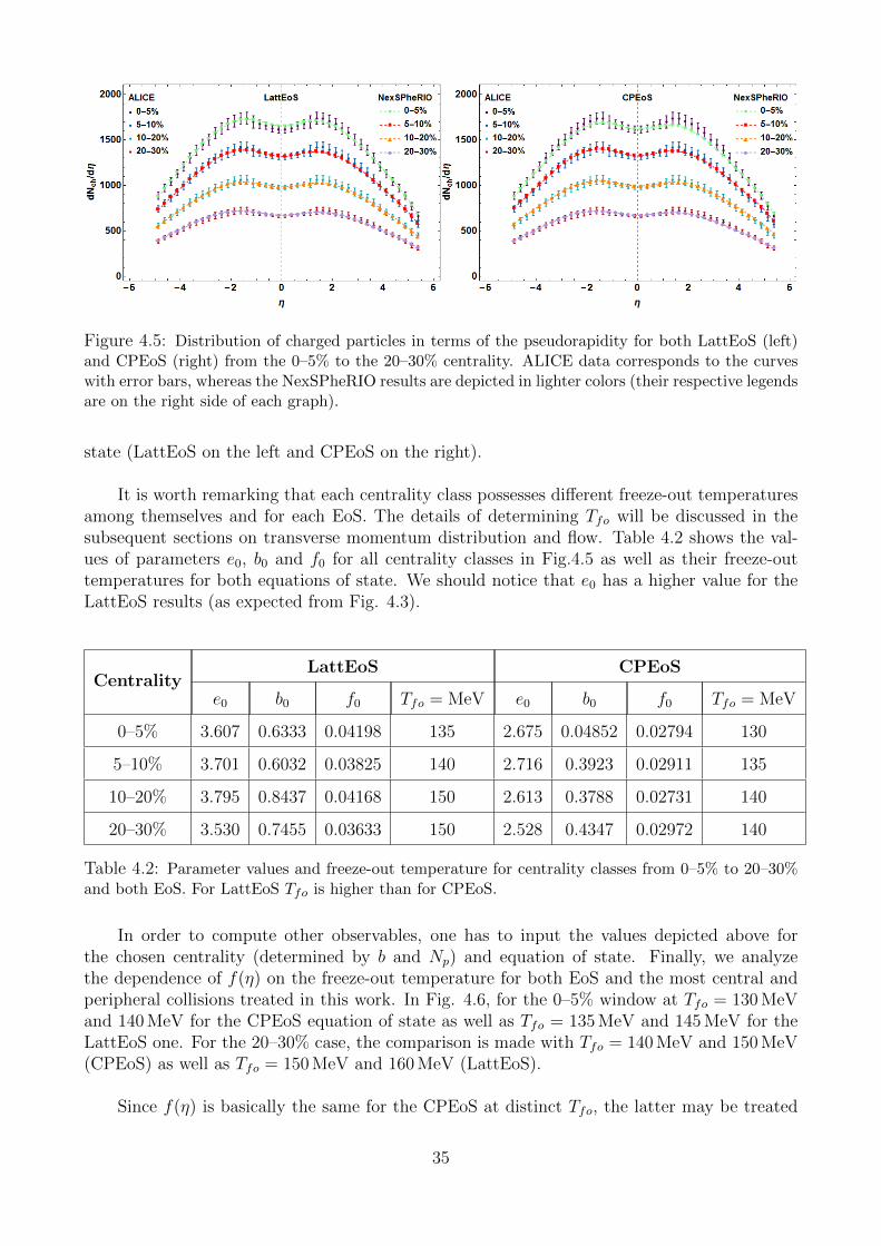
Figure 4.5: Distribution of charged particles in terms of the pseudorapidity for both LattEoS (left)and CPEoS (right) from the 0–5% to the 20–30% centrality. ALICE data corresponds to the curveswith error bars, whereas the NexSPheRIO results are depicted in lighter colors (their respective legendsare on the right side of each graph).

state (LattEoS on the left and CPEoS on the right).

It is worth remarking that each centrality class possesses different freeze-out temperaturesamong themselves and for each EoS. The details of determining Tfo will be discussed in thesubsequent sections on transverse momentum distribution and flow. Table 4.2 shows the val-ues of parameters e0, b0 and f0 for all centrality classes in Fig.4.5 as well as their freeze-outtemperatures for both equations of state. We should notice that e0 has a higher value for theLattEoS results (as expected from Fig. 4.3).

CentralityLattEoS CPEoS

e0 b0 f0 Tfo = MeV e0 b0 f0 Tfo = MeV

0–5% 3.607 0.6333 0.04198 135 2.675 0.04852 0.02794 130

5–10% 3.701 0.6032 0.03825 140 2.716 0.3923 0.02911 135

10–20% 3.795 0.8437 0.04168 150 2.613 0.3788 0.02731 140

20–30% 3.530 0.7455 0.03633 150 2.528 0.4347 0.02972 140

Table 4.2: Parameter values and freeze-out temperature for centrality classes from 0–5% to 20–30%and both EoS. For LattEoS Tfo is higher than for CPEoS.

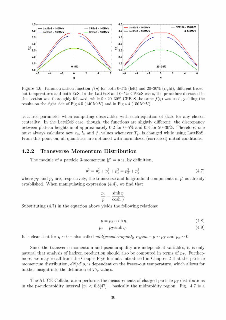
In order to compute other observables, one has to input the values depicted above forthe chosen centrality (determined by b and Np) and equation of state. Finally, we analyzethe dependence of f(η) on the freeze-out temperature for both EoS and the most central andperipheral collisions treated in this work. In Fig. 4.6, for the 0–5% window at Tfo = 130 MeVand 140 MeV for the CPEoS equation of state as well as Tfo = 135 MeV and 145 MeV for theLattEoS one. For the 20–30% case, the comparison is made with Tfo = 140 MeV and 150 MeV(CPEoS) as well as Tfo = 150 MeV and 160 MeV (LattEoS).

Since f(η) is basically the same for the CPEoS at distinct Tfo, the latter may be treated

35

0-5%

LattEoS - 145MeV

LattEoS - 135MeV

CPEoS - 140MeV

CPEoS - 130MeV

-6 -4 -2 0 2 4 61.0

1.5

2.0

2.5

3.0

3.5

4.0

4.5

η

f(η)

20-30%

& 140MeV

LattEoS - 160MeV

LattEoS - 150MeV

CPEoS - 150MeV

-6 -4 -2 0 2 4 61.0

1.5

2.0

2.5

3.0

3.5

4.0

4.5

η

f(η)

Figure 4.6: Parametrization function f(η) for both 0–5% (left) and 20–30% (right), different freeze-out temperatures and both EoS. In the LattEoS and 0–5% CPEoS cases, the procedure discussed inthis section was thoroughly followed, while for 20–30% CPEoS the same f(η) was used, yielding theresults on the right side of Fig.4.5 (140 MeV) and in Fig.4.4 (150 MeV).

as a free parameter when computing observables with such equation of state for any chosencentrality. In the LattEoS case, though, the functions are slightly different: the discrepancybetween plateau heights is of approximately 0.2 for 0–5% and 0.3 for 20–30%. Therefore, onemust always calculate new e0, b0 and f0 values whenever Tfo is changed while using LattEoS.From this point on, all quantities are obtained with normalized (corrected) initial conditions.

4.2.2 Transverse Momentum Distribution

The module of a particle 3-momentum |~p| = p is, by definition,

p2 = p2x + p2

y + p2z = p2

T + p2z, (4.7)

where pT and pz are, respectively, the transverse and longitudinal components of ~p, as alreadyestablished. When manipulating expression (4.4), we find that

pzp

=sinh η

cosh η.

Substituting (4.7) in the equation above yields the following relations:

p = pT cosh η, (4.8)

pz = pT sinh η. (4.9)

It is clear that for η ∼ 0 – also called mid(pseudo)rapidity region – p ∼ pT and pz ∼ 0.

Since the transverse momentum and pseudorapidity are independent variables, it is onlynatural that analysis of hadron production should also be computed in terms of pT . Further-more, we may recall from the Cooper-Frye formula introduced in Chapter 2 that the particlemomentum distribution, dN/d3p, is dependent on the freeze-out temperature, which allows forfurther insight into the definition of Tfo values.

The ALICE Collaboration performs the measurements of charged particle pT distributionsin the pseudorapidity interval |η| < 0.8[47] – basically the midrapidity region. Fig. 4.7 is a

36

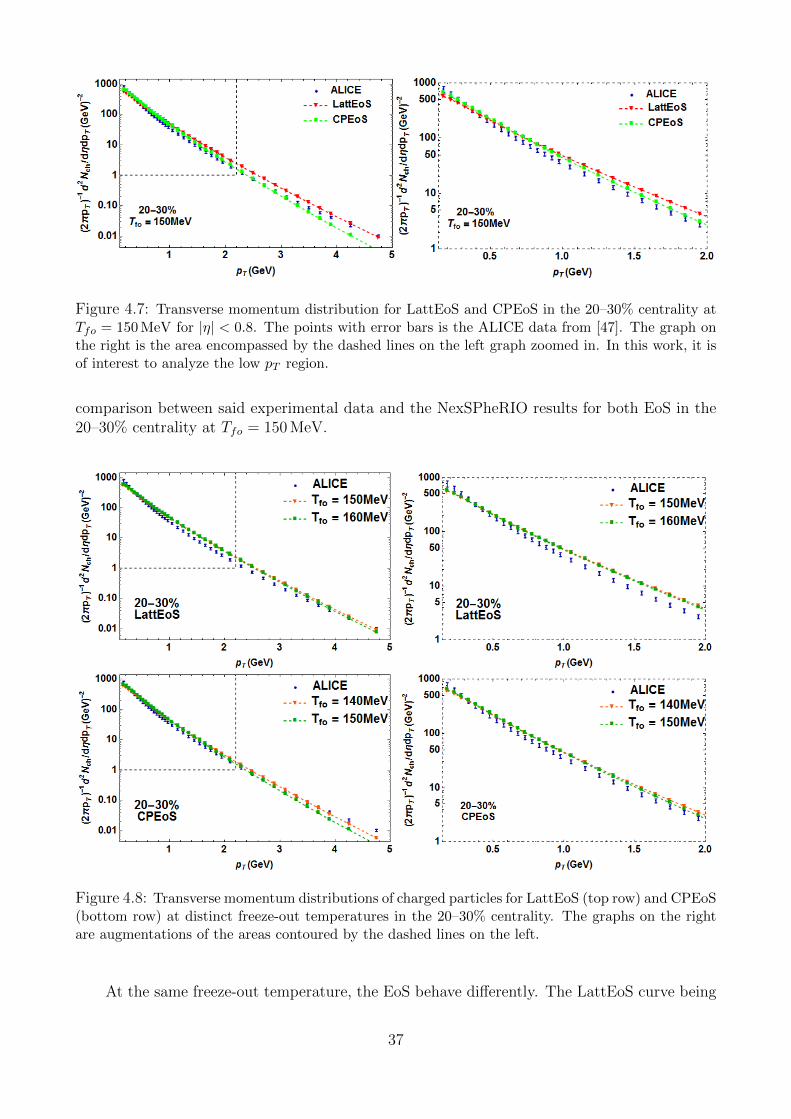
Figure 4.7: Transverse momentum distribution for LattEoS and CPEoS in the 20–30% centrality atTfo = 150 MeV for |η| < 0.8. The points with error bars is the ALICE data from [47]. The graph onthe right is the area encompassed by the dashed lines on the left graph zoomed in. In this work, it isof interest to analyze the low pT region.

comparison between said experimental data and the NexSPheRIO results for both EoS in the20–30% centrality at Tfo = 150 MeV.

Figure 4.8: Transverse momentum distributions of charged particles for LattEoS (top row) and CPEoS(bottom row) at distinct freeze-out temperatures in the 20–30% centrality. The graphs on the rightare augmentations of the areas contoured by the dashed lines on the left.

At the same freeze-out temperature, the EoS behave differently. The LattEoS curve being

37

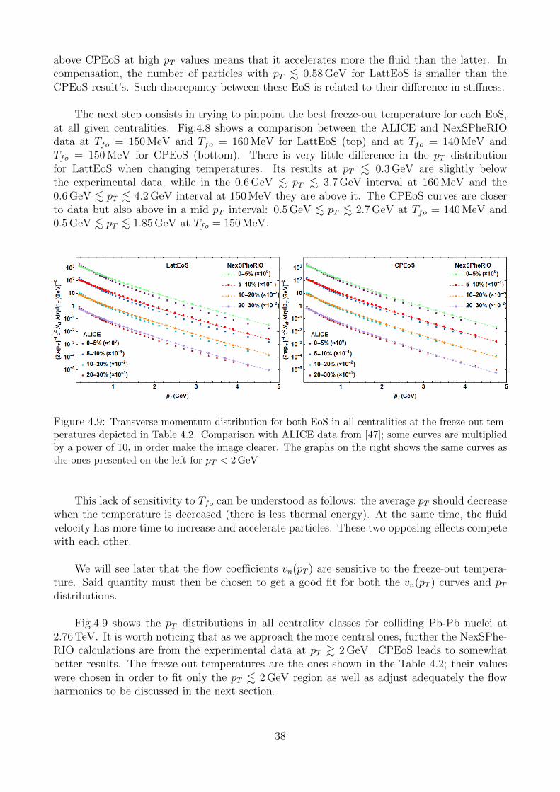
above CPEoS at high pT values means that it accelerates more the fluid than the latter. Incompensation, the number of particles with pT . 0.58 GeV for LattEoS is smaller than theCPEoS result’s. Such discrepancy between these EoS is related to their difference in stiffness.

The next step consists in trying to pinpoint the best freeze-out temperature for each EoS,at all given centralities. Fig.4.8 shows a comparison between the ALICE and NexSPheRIOdata at Tfo = 150 MeV and Tfo = 160 MeV for LattEoS (top) and at Tfo = 140 MeV andTfo = 150 MeV for CPEoS (bottom). There is very little difference in the pT distributionfor LattEoS when changing temperatures. Its results at pT . 0.3 GeV are slightly belowthe experimental data, while in the 0.6 GeV . pT . 3.7 GeV interval at 160 MeV and the0.6 GeV . pT . 4.2 GeV interval at 150 MeV they are above it. The CPEoS curves are closerto data but also above in a mid pT interval: 0.5 GeV . pT . 2.7 GeV at Tfo = 140 MeV and0.5 GeV . pT . 1.85 GeV at Tfo = 150 MeV.

Figure 4.9: Transverse momentum distribution for both EoS in all centralities at the freeze-out tem-peratures depicted in Table 4.2. Comparison with ALICE data from [47]; some curves are multipliedby a power of 10, in order make the image clearer. The graphs on the right shows the same curves asthe ones presented on the left for pT < 2 GeV

This lack of sensitivity to Tfo can be understood as follows: the average pT should decreasewhen the temperature is decreased (there is less thermal energy). At the same time, the fluidvelocity has more time to increase and accelerate particles. These two opposing effects competewith each other.

We will see later that the flow coefficients vn(pT ) are sensitive to the freeze-out tempera-ture. Said quantity must then be chosen to get a good fit for both the vn(pT ) curves and pTdistributions.

Fig.4.9 shows the pT distributions in all centrality classes for colliding Pb-Pb nuclei at2.76 TeV. It is worth noticing that as we approach the more central ones, further the NexSPhe-RIO calculations are from the experimental data at pT & 2 GeV. CPEoS leads to somewhatbetter results. The freeze-out temperatures are the ones shown in the Table 4.2; their valueswere chosen in order to fit only the pT . 2 GeV region as well as adjust adequately the flowharmonics to be discussed in the next section.

38

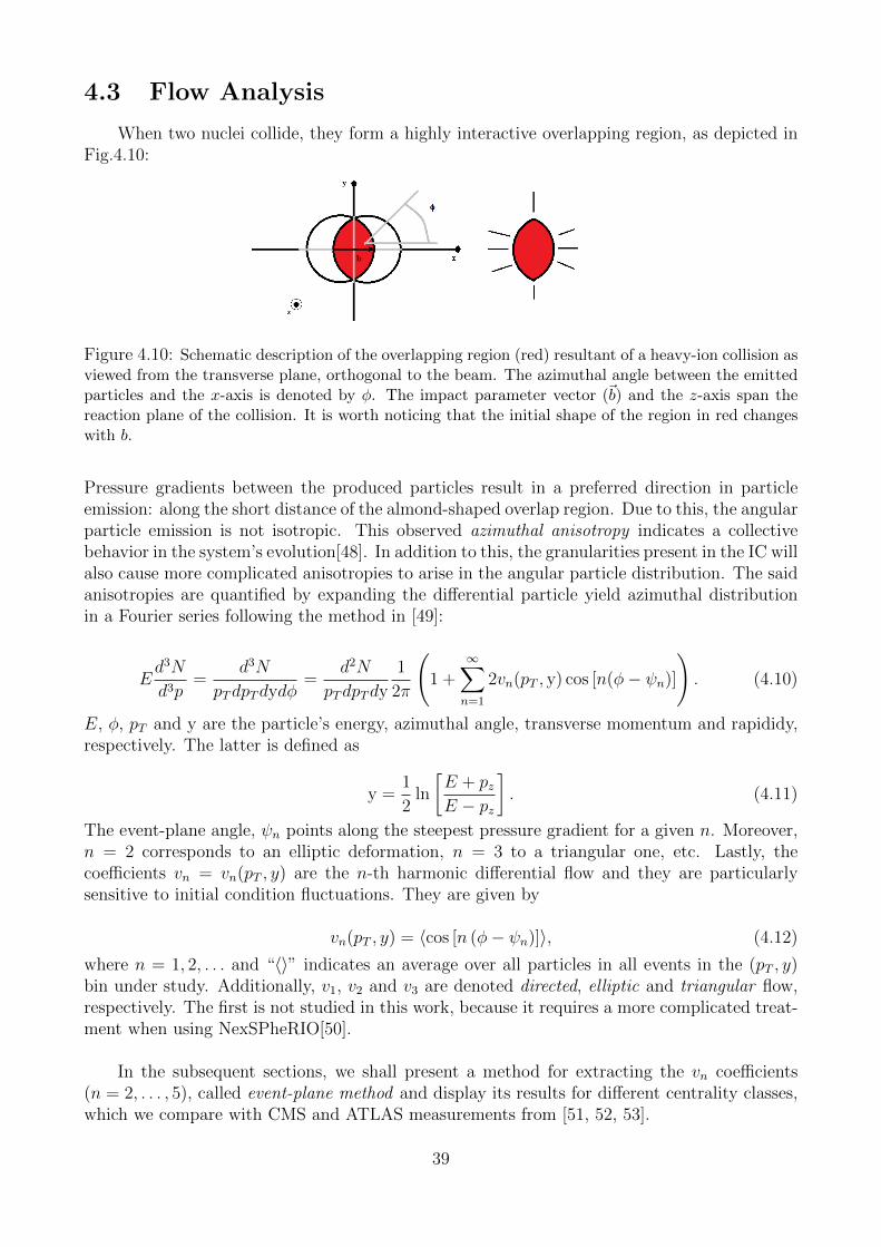
4.3 Flow Analysis

When two nuclei collide, they form a highly interactive overlapping region, as depicted inFig.4.10:

Figure 4.10: Schematic description of the overlapping region (red) resultant of a heavy-ion collision asviewed from the transverse plane, orthogonal to the beam. The azimuthal angle between the emittedparticles and the x-axis is denoted by φ. The impact parameter vector (~b) and the z-axis span thereaction plane of the collision. It is worth noticing that the initial shape of the region in red changeswith b.

Pressure gradients between the produced particles result in a preferred direction in particleemission: along the short distance of the almond-shaped overlap region. Due to this, the angularparticle emission is not isotropic. This observed azimuthal anisotropy indicates a collectivebehavior in the system’s evolution[48]. In addition to this, the granularities present in the IC willalso cause more complicated anisotropies to arise in the angular particle distribution. The saidanisotropies are quantified by expanding the differential particle yield azimuthal distributionin a Fourier series following the method in [49]:

Ed3N

d3p=

d3N

pTdpTdydφ=

d2N

pTdpTdy

1

2π

(1 +

∞∑n=1

2vn(pT , y) cos [n(φ− ψn)]

). (4.10)

E, φ, pT and y are the particle’s energy, azimuthal angle, transverse momentum and rapididy,respectively. The latter is defined as

y =1

2ln

[E + pzE − pz

]. (4.11)

The event-plane angle, ψn points along the steepest pressure gradient for a given n. Moreover,n = 2 corresponds to an elliptic deformation, n = 3 to a triangular one, etc. Lastly, thecoefficients vn = vn(pT , y) are the n-th harmonic differential flow and they are particularlysensitive to initial condition fluctuations. They are given by

vn(pT , y) = 〈cos [n (φ− ψn)]〉, (4.12)

where n = 1, 2, . . . and “〈〉” indicates an average over all particles in all events in the (pT , y)bin under study. Additionally, v1, v2 and v3 are denoted directed, elliptic and triangular flow,respectively. The first is not studied in this work, because it requires a more complicated treat-ment when using NexSPheRIO[50].

In the subsequent sections, we shall present a method for extracting the vn coefficients(n = 2, . . . , 5), called event-plane method and display its results for different centrality classes,which we compare with CMS and ATLAS measurements from [51, 52, 53].

39

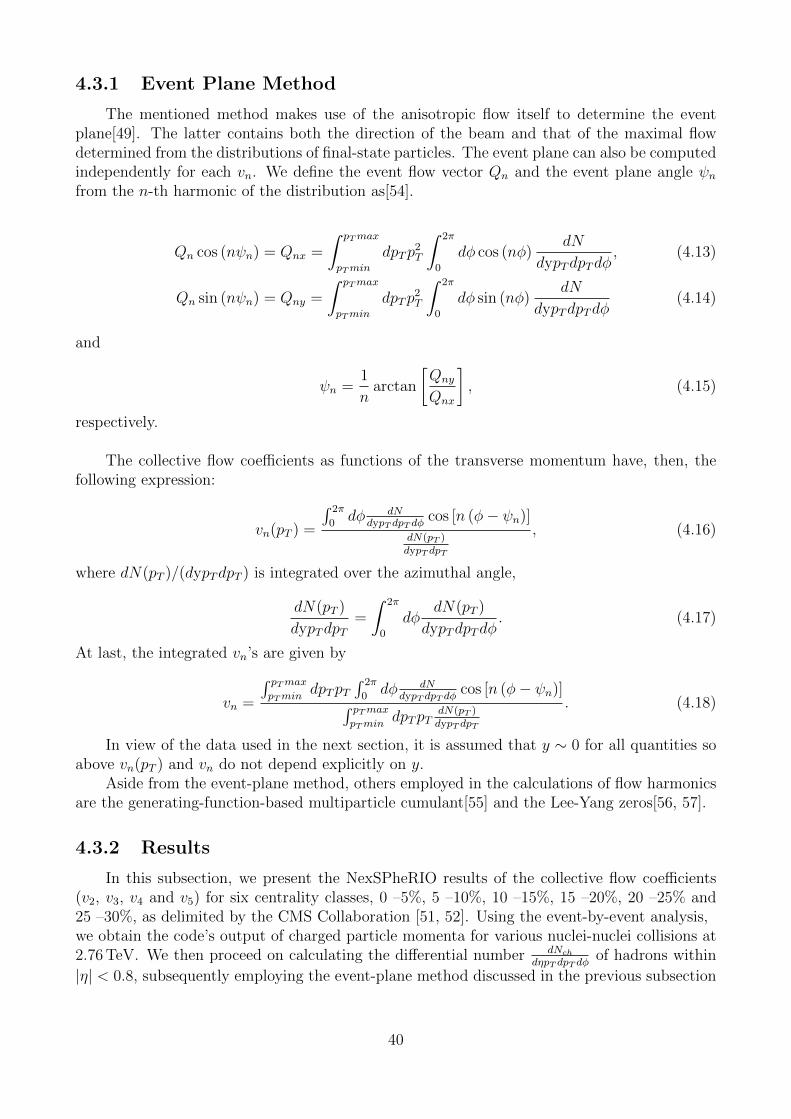
4.3.1 Event Plane Method

The mentioned method makes use of the anisotropic flow itself to determine the eventplane[49]. The latter contains both the direction of the beam and that of the maximal flowdetermined from the distributions of final-state particles. The event plane can also be computedindependently for each vn. We define the event flow vector Qn and the event plane angle ψnfrom the n-th harmonic of the distribution as[54].

Qn cos (nψn) = Qnx =

∫ pTmax

pTmin

dpTp2T

∫ 2π

0

dφ cos (nφ)dN

dypTdpTdφ, (4.13)

Qn sin (nψn) = Qny =

∫ pTmax

pTmin

dpTp2T

∫ 2π

0

dφ sin (nφ)dN

dypTdpTdφ(4.14)

and

ψn =1

narctan

[Qny

Qnx

], (4.15)

respectively.

The collective flow coefficients as functions of the transverse momentum have, then, thefollowing expression:

vn(pT ) =

∫ 2π

0dφ dN

dypT dpT dφcos [n (φ− ψn)]

dN(pT )dypT dpT

, (4.16)

where dN(pT )/(dypTdpT ) is integrated over the azimuthal angle,

dN(pT )

dypTdpT=

∫ 2π

0

dφdN(pT )

dypTdpTdφ. (4.17)

At last, the integrated vn’s are given by

vn =

∫ pTmaxpTmin

dpTpT∫ 2π

0dφ dN

dypT dpT dφcos [n (φ− ψn)]∫ pTmax

pTmindpTpT

dN(pT )dypT dpT

. (4.18)

In view of the data used in the next section, it is assumed that y ∼ 0 for all quantities soabove vn(pT ) and vn do not depend explicitly on y.

Aside from the event-plane method, others employed in the calculations of flow harmonicsare the generating-function-based multiparticle cumulant[55] and the Lee-Yang zeros[56, 57].

4.3.2 Results

In this subsection, we present the NexSPheRIO results of the collective flow coefficients(v2, v3, v4 and v5) for six centrality classes, 0 –5%, 5 –10%, 10 –15%, 15 –20%, 20 –25% and25 –30%, as delimited by the CMS Collaboration [51, 52]. Using the event-by-event analysis,we obtain the code’s output of charged particle momenta for various nuclei-nuclei collisions at2.76 TeV. We then proceed on calculating the differential number dNch

dηpT dpT dφof hadrons within

|η| < 0.8, subsequently employing the event-plane method discussed in the previous subsection

40

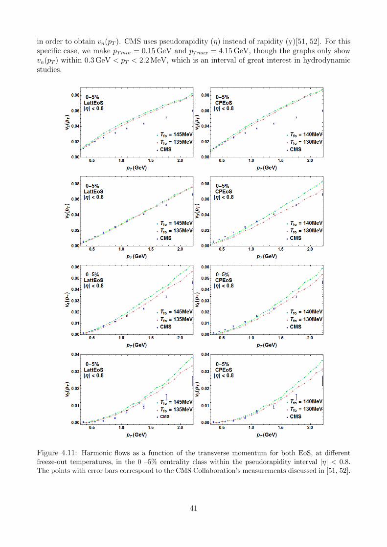
in order to obtain vn(pT ). CMS uses pseudorapidity (η) instead of rapidity (y)[51, 52]. For thisspecific case, we make pTmin = 0.15 GeV and pTmax = 4.15 GeV, though the graphs only showvn(pT ) within 0.3 GeV < pT < 2.2 MeV, which is an interval of great interest in hydrodynamicstudies.

Figure 4.11: Harmonic flows as a function of the transverse momentum for both EoS, at differentfreeze-out temperatures, in the 0 –5% centrality class within the pseudorapidity interval |η| < 0.8.The points with error bars correspond to the CMS Collaboration’s measurements discussed in [51, 52].

41

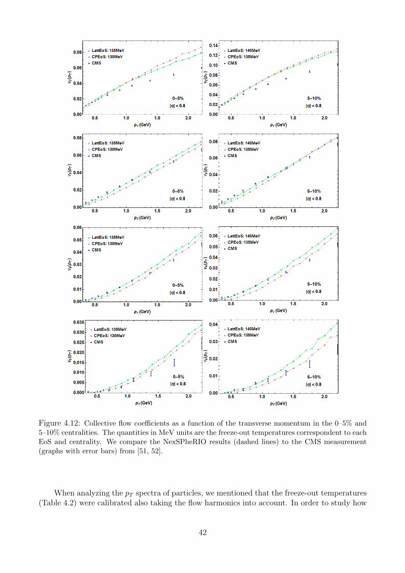
Figure 4.12: Collective flow coefficients as a function of the transverse momentum in the 0–5% and5–10% centralities. The quantities in MeV units are the freeze-out temperatures correspondent to eachEoS and centrality. We compare the NexSPheRIO results (dashed lines) to the CMS measurement(graphs with error bars) from [51, 52].

When analyzing the pT spectra of particles, we mentioned that the freeze-out temperatures(Table 4.2) were calibrated also taking the flow harmonics into account. In order to study how

42

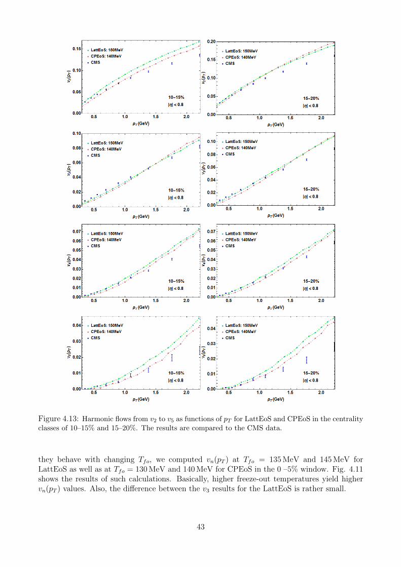
Figure 4.13: Harmonic flows from v2 to v5 as functions of pT for LattEoS and CPEoS in the centralityclasses of 10–15% and 15–20%. The results are compared to the CMS data.

they behave with changing Tfo, we computed vn(pT ) at Tfo = 135 MeV and 145 MeV forLattEoS as well as at Tfo = 130 MeV and 140 MeV for CPEoS in the 0 –5% window. Fig. 4.11shows the results of such calculations. Basically, higher freeze-out temperatures yield highervn(pT ) values. Also, the difference between the v3 results for the LattEoS is rather small.

43

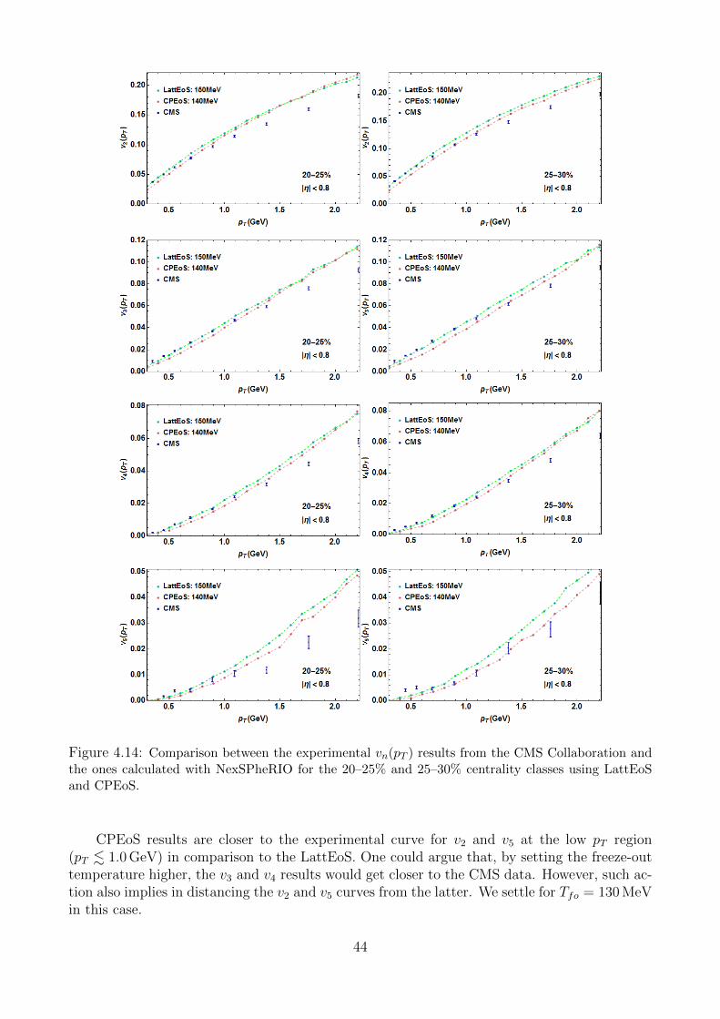
Figure 4.14: Comparison between the experimental vn(pT ) results from the CMS Collaboration andthe ones calculated with NexSPheRIO for the 20–25% and 25–30% centrality classes using LattEoSand CPEoS.

CPEoS results are closer to the experimental curve for v2 and v5 at the low pT region(pT . 1.0 GeV) in comparison to the LattEoS. One could argue that, by setting the freeze-outtemperature higher, the v3 and v4 results would get closer to the CMS data. However, such ac-tion also implies in distancing the v2 and v5 curves from the latter. We settle for Tfo = 130 MeVin this case.

44

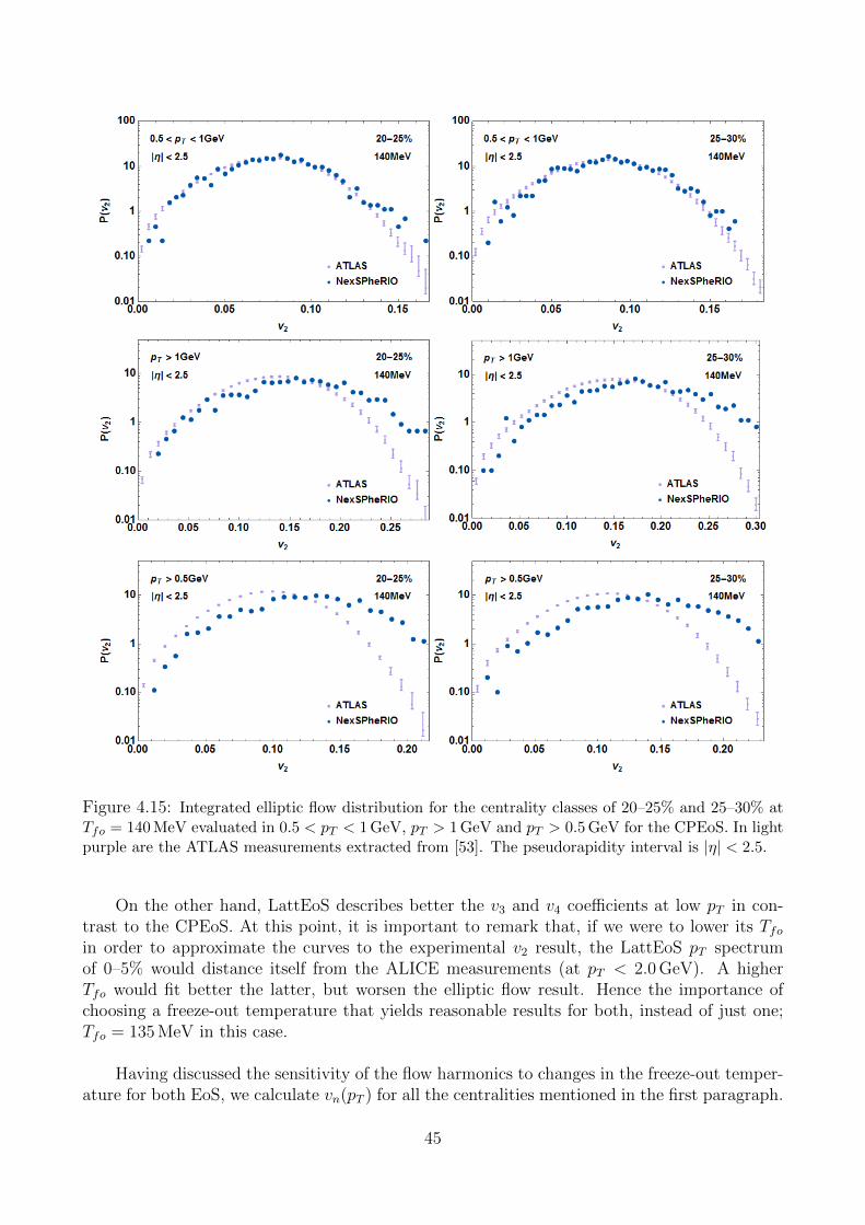
Figure 4.15: Integrated elliptic flow distribution for the centrality classes of 20–25% and 25–30% atTfo = 140 MeV evaluated in 0.5 < pT < 1 GeV, pT > 1 GeV and pT > 0.5 GeV for the CPEoS. In lightpurple are the ATLAS measurements extracted from [53]. The pseudorapidity interval is |η| < 2.5.

On the other hand, LattEoS describes better the v3 and v4 coefficients at low pT in con-trast to the CPEoS. At this point, it is important to remark that, if we were to lower its Tfoin order to approximate the curves to the experimental v2 result, the LattEoS pT spectrumof 0–5% would distance itself from the ALICE measurements (at pT < 2.0 GeV). A higherTfo would fit better the latter, but worsen the elliptic flow result. Hence the importance ofchoosing a freeze-out temperature that yields reasonable results for both, instead of just one;Tfo = 135 MeV in this case.

Having discussed the sensitivity of the flow harmonics to changes in the freeze-out temper-ature for both EoS, we calculate vn(pT ) for all the centralities mentioned in the first paragraph.

45

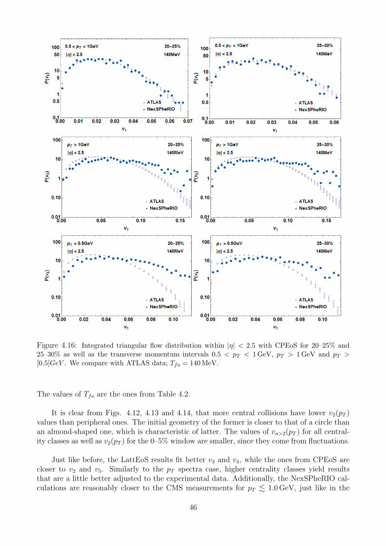
Figure 4.16: Integrated triangular flow distribution within |η| < 2.5 with CPEoS for 20–25% and25–30% as well as the transverse momentum intervals 0.5 < pT < 1 GeV, pT > 1 GeV and pT >[0.5]GeV . We compare with ATLAS data; Tfo = 140 MeV.

The values of Tfo are the ones from Table 4.2.

It is clear from Figs. 4.12, 4.13 and 4.14, that more central collisions have lower v2(pT )values than peripheral ones. The initial geometry of the former is closer to that of a circle thanan almond-shaped one, which is characteristic of latter. The values of vn>2(pT ) for all central-ity classes as well as v2(pT ) for the 0–5% window are smaller, since they come from fluctuations.

Just like before, the LattEoS results fit better v3 and v4, while the ones from CPEoS arecloser to v2 and v5. Similarly to the pT spectra case, higher centrality classes yield resultsthat are a little better adjusted to the experimental data. Additionally, the NexSPheRIO cal-culations are reasonably closer to the CMS measurements for pT . 1.0 GeV, just like in the

46

Figure 4.17: Distribution of the integrated collective flow coefficient, v4 for 20–25% and 25–30% atTfo = 140 MeV. Just like in the P (v2) and P (v3) calculations, we employed the CPEoS and computedthe particle spectrum within the 0.5 < pT < 1 GeV, pT > 1 GeV and pT > 0.5 Gev intervals. ATLASis represented by the light purple points; |η| < 2.5.

transverse momentum distribution comparisons.

So far, we have discussed vn(pT ) averaged over events. In order to study more closelythe IC fluctuations, it is interesting to look at the pT -integrated vn’s. So, our last step in theflow analysis consists in computing the integrated vn’s as in eq. (4.18). We then calculatethe distributions of the flow harmonic coefficients vn (n = 2, 3, 4) for charged particles with0.5 GeV < pT < 1.0 Gev, pT > 1.0 GeV and pT > 0.5 GeV in the |η| < 2.5 interval, as measuredby the ALTLAS Collaboration in [53]. The aforementioned is performed for the 20–25% and25–30% centrality classes with the CPEoS and Tfo = 140 MeV. We ran 1109 events for theformer and 1233 for the latter.

47

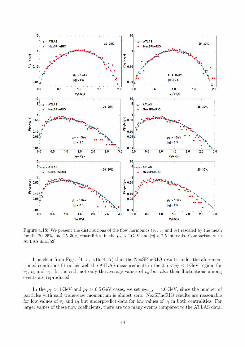
Figure 4.18: We present the distributions of the flow harmonics (v2, v3 and v4) rescaled by the meanfor the 20–25% and 25–30% centralities, in the pT > 1 GeV and |η| < 2.5 intervals. Comparison withATLAS data[53].

It is clear from Figs. (4.15, 4.16, 4.17) that the NexSPheRIO results under the aforemen-tioned conditions fit rather well the ATLAS measurements in the 0.5 < pT < 1 GeV region, forv2, v3 and v4. In the end, not only the average values of vn but also their fluctuations amongevents are reproduced.

In the pT > 1 GeV and pT > 0.5 GeV cases, we set pTmax = 4.0 GeV, since the number ofparticles with said transverse momentum is almost zero. NexSPheRIO results are reasonablefor low values of v2 and v3 but underpredict data for low values of v4 in both centralities. Forlarger values of these flow coefficients, there are too many events compared to the ATLAS data.

48

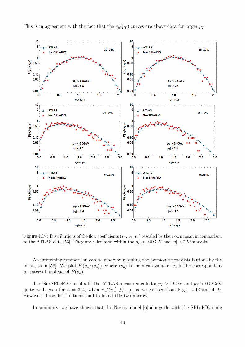
This is in agreement with the fact that the vn(pT ) curves are above data for larger pT .

Figure 4.19: Distributions of the flow coefficients (v2, v3, v4) rescaled by their own mean in comparisonto the ATLAS data [53]. They are calculated within the pT > 0.5 GeV and |η| < 2.5 intervals.

An interesting comparison can be made by rescaling the harmonic flow distributions by themean, as in [58]. We plot P (vn/〈vn〉), where 〈vn〉 is the mean value of vn in the correspondentpT interval, instead of P (vn).

The NexSPheRIO results fit the ATLAS measurements for pT > 1 GeV and pT > 0.5 GeVquite well, even for n = 3, 4, when vn/〈vn〉 . 1.5, as we can see from Figs. 4.18 and 4.19.However, these distributions tend to be a little two narrow.

In summary, we have shown that the Nexus model [6] alongside with the SPheRIO code

49

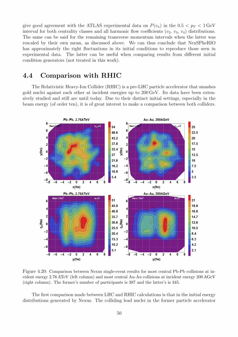
give good agreement with the ATLAS experimental data on P (vn) in the 0.5 < pT < 1 GeVinterval for both centrality classes and all harmonic flow coefficients (v2, v3, v4) distributions.The same can be said for the remaining transverse momentum intervals when the latter wasrescaled by their own mean, as discussed above. We can thus conclude that NexSPheRIOhas approximately the right fluctuations in its initial conditions to reproduce those seen inexperimental data. The latter can be useful when comparing results from different initialcondition generators (not treated in this work).

4.4 Comparison with RHIC

The Relativistic Heavy-Ion Collider (RHIC) is a pre-LHC particle accelerator that smashesgold nuclei against each other at incident energies up to 200 GeV. Its data have been exten-sively studied and still are until today. Due to their distinct initial settings, especially in thebeam energy (of order ten), it is of great interest to make a comparison between both colliders.

Figure 4.20: Comparison between Nexus single-event results for most central Pb-Pb collisions at in-cident energy 2.76 ATeV (left column) and most central Au-Au collisions at incident energy 200 AGeV(right column). The former’s number of participants is 387 and the latter’s is 345.

The first comparison made between LHC and RHIC calculations is that in the initial energydistributions generated by Nexus. The colliding lead nuclei in the former particle accelerator

50

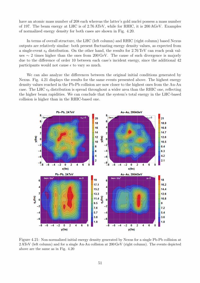
have an atomic mass number of 208 each whereas the latter’s gold nuclei possess a mass numberof 197. The beam energy at LHC is of 2.76 ATeV, while for RHIC, it is 200 AGeV. Examplesof normalized energy density for both cases are shown in Fig. 4.20.

In terms of overall structure, the LHC (left column) and RHIC (right column) based Nexusoutputs are relatively similar: both present fluctuating energy density values, as expected froma single-event ε0 distribution. On the other hand, the results for 2.76 TeV can reach peak val-ues ∼ 2 times higher than the ones from 200 GeV. The cause of such divergence is majorlydue to the difference of order 10 between each case’s incident energy, since the additional 42participants would not cause ε to vary so much.

We can also analyze the differences between the original initial conditions generated byNexus. Fig. 4.21 displays the results for the same events presented above. The highest energydensity values reached in the Pb-Pb collision are now closer to the highest ones from the Au-Aucase. The LHC ε0 distribution is spread throughout a wider area than the RHIC one, reflectingthe higher beam rapidities. We can conclude that the system’s total energy in the LHC-basedcollision is higher than in the RHIC-based one.

Figure 4.21: Non-normalized initial energy density generated by Nexus for a single Pb-Pb collision at2 ATeV (left column) and for a single Au-Au collision at 200 GeV (right column). The events depictedabove are the same as in Fig. 4.20

51

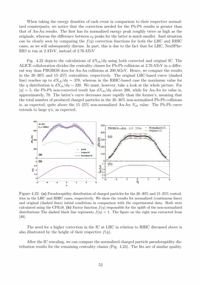
When taking the energy densities of each event in comparison to their respective normal-ized counterparts, we notice that the correction needed for the Pb-Pb results is greater thanthat of Au-Au results. The first has its normalized energy peak roughly twice as high as theoriginals, whereas the difference between ε0 peaks for the latter is much smaller. Said situationcan be clearly seen by comparing the f(η) correction functions for both the LHC and RHICcases, as we will subsequently discuss. In part, this is due to the fact that for LHC, NexSPhe-RIO is run at 2 ATeV, instead of 2.76 ATeV

Fig. 4.22 depicts the calculations of dNch/dη using both corrected and original IC. TheALICE collaboration divides the centrality classes for Pb-Pb collisions at 2.76 ATeV in a differ-ent way than PHOBOS does for Au-Au collisions at 200 AGeV. Hence, we compare the resultsin the 20–30% and 15–25% centralities, respectively. The original LHC-based curve (dashedline) reaches up to dNch/dη ∼ 370, whereas in the RHIC-based case the maximum value forthe η distribution is dNch/dη ∼ 320. We must, however, take a look at the whole picture. For|η| = 5, the Pb-Pb non-corrected result has dNch/dη above 200, while for Au-Au its value is,approximately, 70. The latter’s curve decreases more rapidly than the former’s, meaning thatthe total number of produced charged particles in the 20–30% non-normalized Pb-Pb collisionsis, as expected, quite above the 15–25% non-normalized Au-Au Nch value. The Pb-Pb curveextends to large η’s, as expected.

Figure 4.22: (a) Pseudorapidity distribution of charged particles for the 20–30% and 15–25% central-ities in the LHC and RHIC cases, respectively. We show the results for normalized (continuous lines)and original (dashed lines) initial conditions in comparison with the experimental data. Both werecalculated using the CPEoS. (b) Factor function f(η) responsible for the uplift of the non-normalizeddistributions The dashed black line represents f(η) = 1. The figure on the right was extracted from[40].

The need for a higher correction in the IC at LHC in relation to RHIC discussed above isalso illustrated by the height of their respective f(η).

After the IC rescaling, we can compare the normalized charged particle pseudorapidity dis-tribution results for the remaining centrality classes (Fig. 4.23). The fits are of similar quality.

52

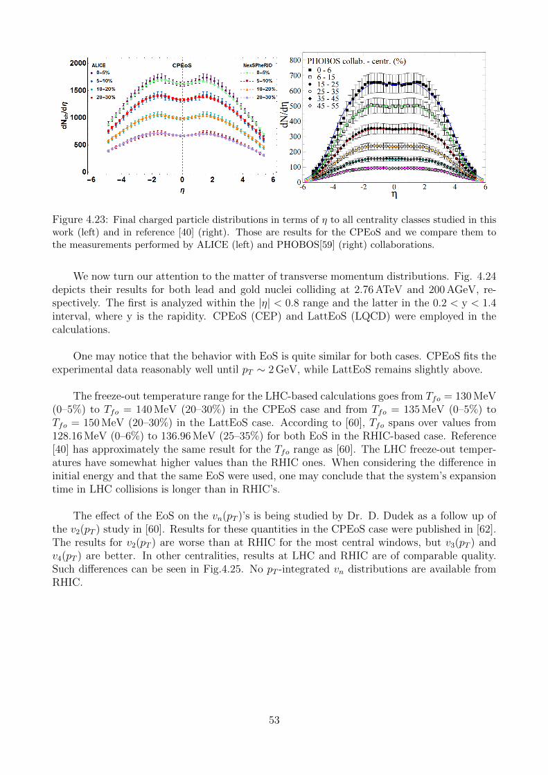
Figure 4.23: Final charged particle distributions in terms of η to all centrality classes studied in thiswork (left) and in reference [40] (right). Those are results for the CPEoS and we compare them tothe measurements performed by ALICE (left) and PHOBOS[59] (right) collaborations.

We now turn our attention to the matter of transverse momentum distributions. Fig. 4.24depicts their results for both lead and gold nuclei colliding at 2.76 ATeV and 200 AGeV, re-spectively. The first is analyzed within the |η| < 0.8 range and the latter in the 0.2 < y < 1.4interval, where y is the rapidity. CPEoS (CEP) and LattEoS (LQCD) were employed in thecalculations.

One may notice that the behavior with EoS is quite similar for both cases. CPEoS fits theexperimental data reasonably well until pT ∼ 2 GeV, while LattEoS remains slightly above.

The freeze-out temperature range for the LHC-based calculations goes from Tfo = 130 MeV(0–5%) to Tfo = 140 MeV (20–30%) in the CPEoS case and from Tfo = 135 MeV (0–5%) toTfo = 150 MeV (20–30%) in the LattEoS case. According to [60], Tfo spans over values from128.16 MeV (0–6%) to 136.96 MeV (25–35%) for both EoS in the RHIC-based case. Reference[40] has approximately the same result for the Tfo range as [60]. The LHC freeze-out temper-atures have somewhat higher values than the RHIC ones. When considering the difference ininitial energy and that the same EoS were used, one may conclude that the system’s expansiontime in LHC collisions is longer than in RHIC’s.

The effect of the EoS on the vn(pT )’s is being studied by Dr. D. Dudek as a follow up ofthe v2(pT ) study in [60]. Results for these quantities in the CPEoS case were published in [62].The results for v2(pT ) are worse than at RHIC for the most central windows, but v3(pT ) andv4(pT ) are better. In other centralities, results at LHC and RHIC are of comparable quality.Such differences can be seen in Fig.4.25. No pT -integrated vn distributions are available fromRHIC.

53

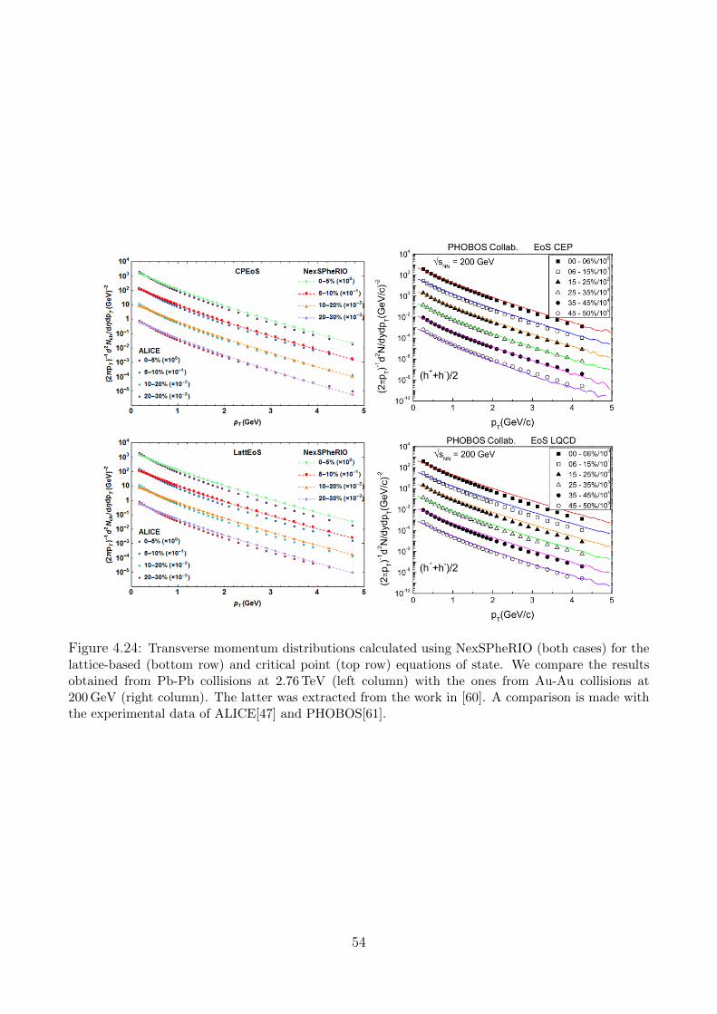
Figure 4.24: Transverse momentum distributions calculated using NexSPheRIO (both cases) for thelattice-based (bottom row) and critical point (top row) equations of state. We compare the resultsobtained from Pb-Pb collisions at 2.76 TeV (left column) with the ones from Au-Au collisions at200 GeV (right column). The latter was extracted from the work in [60]. A comparison is made withthe experimental data of ALICE[47] and PHOBOS[61].

54

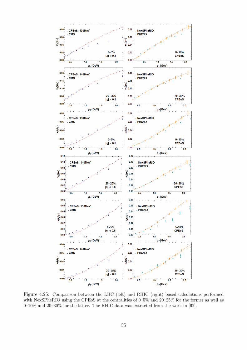
Figure 4.25: Comparison between the LHC (left) and RHIC (right) based calculations performedwith NexSPheRIO using the CPEoS at the centralities of 0–5% and 20–25% for the former as well as0–10% and 20–30% for the latter. The RHIC data was extracted from the work in [62].

55

Chapter 5

Conclusion

In this work, we applied event-by-event hydrodynamics in order to simulate the LHCheavy-ion experiments: lead nuclei colliding at incident energy of 2.76 ATeV. When perform-ing such task, one must determine a set of ingredients, such as the system’s initial conditions(IC), the equation of state that dictates the relations between the thermodynamic variablesand the freeze-out scenario. We generated the IC by making use of the Nexus model, whichgives as output the energy-momentum tensor as well as the baryon, strangeness and electriccharge currents. Secondly, two distinct EoS were discussed, one with µB 6= 0, characterized bya critical point ((µB)c, Tc) where the phase transition changes from first-order to a crossovertype (CPEoS) and a baryonless LatticeQCD-based one (LattEoS). Finally, we adopted theCooper-Frye decoupling mechanism, for which the particles momenta freeze after crossing ahypersurface defined by the isotherm T (t, x, y, z) = Tfo. The next step consisted in solving theequations of motion of hydrodynamics (introduced in section 2.1) by making use of the SPHmethod.

With the main ingredients and computing method established, we moved on to making ananalysis of the relation between impact parameter (b) and number of participants in a collision(Np), in order to define their values for each centrality class. The latter were divided as inthe ALICE collaboration [46, 47]. Being able to “choose” how central or peripheral a collisionwould be, we then ran the NexSPheRIO code at 2 ATeV, thus obtaining first the results oncharged particle distributions in terms of pseudorapidity. Since the aforementioned had insuf-ficient initial energy to produce the expected number of particles, we introduced a correctionfunction dependent on η with the objective of normalizing the Nexus-generated IC to be usableat the 2.76 TeV beam energy. The parameters of f(η) were calculated for the most centralcollisions (0–30%) and claimed different values for each EoS. The latter were also found to havedistinct freeze-out temperatures at given centrality. The final dNch/dη plots fit satisfactorilythe ALICE experimental data.

The effect of Tfo in the particle spectra was then observed when we computed the chargedparticle distribution in terms of transverse momentum in the |η| < 0.8 region. The LattEoScurve ended up being less steep than the CPEoS one at a given freeze-out temperature. Theformer’s result fit the ALICE measurements reasonably well for pT . 1 GeV, whereas the latterdid the same for pT . 2 GeV. They would adjust quite well to the experimental results in theregion of interest (pT < 2 GeV) the more peripheral were the centralities. The Tfo values weredefined as to best fit the LattEoS and CPEoS curves to the ALICE data on pT distribution,while still giving a reasonable result to the flow harmonics.

56

Having defined the correction function’s parameters as well as the freeze-out temperaturefor each centrality class and EoS, we analyzed how the flow coefficients change with transversemomentum (vn(pT )). By employing the event-plane method, we obtained from the NexSPhe-RIO results on dNch

ypT dpT dφ(|η| < 0.8) the curves for the flow harmonics v2, v3, v4 and v5 as

functions of pT . We found that the vn(pT ) curves get higher with increasing Tfo, in a mannerthat, depending on the chosen value, the graphs could fit either v2 and v5 or v3 and v4 better.Such observation called for a calibration of Tfo, in order to obtain a result that would adjustreasonably to all pT dependent quantities. Overall, the flow coefficient (vn(pT )) calculations forboth EoS at all given centralities were in sensible agreement with the CMS measurements inthe pT . 1 GeV region.

After computing vn(pT ), we looked at integrated vn (n = 2, 3, 4) distributions in the20–25% and 25–30% centrality classes, using CPEoS, for three pT intervals, 0.5 < pT < 1 GeV,pT > 1 GeV and pT > 1 GeV, as well as |η| < 2.5. In the case of 0.5 < pT < 1 GeV, the resultsadjusted well to the ATLAS collaboration measurements, for all flow harmonics at hand. Sincethe same cannot be said for the other two intervals, we rescaled by the mean value 〈vn〉, thuscalculating P (vn)/〈vn〉. We find the curves to fit the rescaled ATLAS data reasonably, thoughthey are a little too narrow for n = 3, 4. This type of calculation had never been done beforefor NexSPheRIO. It shows that not only the code leads to good results for the event-averagedvn(pT )’s, but also has the right amount of fluctuations in its IC to produce the correct vn’s onan event-by-event basis.

Finally, we made comparisons of our results to previous NexSPheRIO calculations forRHIC, which are found in references [40, 60]. We begin by analyzing the Nexus-generated ICfor the most central collisions in both cases. When they are normalized, the energy densitypeaks of Pb-Pb collisions at 2.76 ATeV reaches a factor 2 above e0 that for Au-Au collisions at200 AGeV. The correction that needs to be applied in order to get the normalized IC is largerat LHC than at RHIC (in part due to a technical limitation in NexSPheRIO). The quality ofthe fits to the pseudorapidity distributions then obtained is similar for both colliders.

Subsequently, we compared the results in charged particle distributions in terms of trans-verse momentum in the LHC and RHIC scenarios. We observe that the fits are of similarquality and share common characteristics for changes in centrality and equation of state. Wethen finally argued that the quality of the fits for the vn(pT )’s are not very different, except forv2(pT ) at the most central collisions.

All in all, the NexSPheRIO results of event-by-event hydrodynamics adjust well to themeasurements performed by LHC detectors, ALICE, CMS and ATLAS. This is surprising: itis usually expected that gluon saturation effects should be manifest at LHC and the IC, unlikethe Nexus’ ones, should incorporate this. We note, however, that the present analysis mustbe extended to the remaining centralities and could be done for various particle types, insteadof just charged particles. In addition, we could further the studies on LHC by calculating theHambury-Brown-Twiss (HBT) and Ridge effects, as well as trying out a more sophisticated par-ticle emission scenario: chemical freeze-out, along with continuous emission, transport model.At last, but not least, the effects of shear and bulk viscocities should be assessed.

57

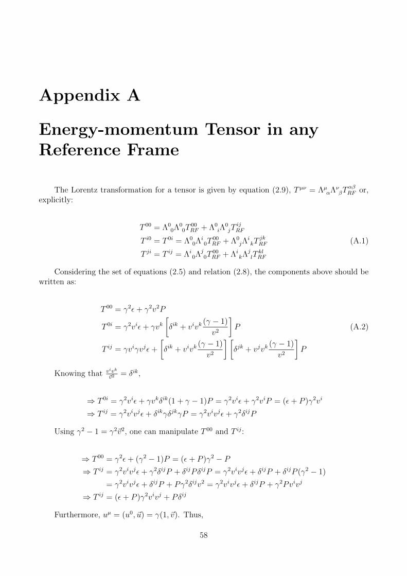
Appendix A

Energy-momentum Tensor in anyReference Frame

The Lorentz transformation for a tensor is given by equation (2.9), T µν = ΛµαΛν

βTαβRF or,

explicitly:

T 00 = Λ00Λ0

0T00RF + Λ0

iΛ0jT

ijRF

T i0 = T 0i = Λ00Λi

0T00RF + Λ0

jΛikT

jkRF (A.1)

T ji = T ij = Λi0Λj

0T00RF + Λi

kΛjlT

klRF

Considering the set of equations (2.5) and relation (2.8), the components above should bewritten as:

T 00 = γ2ε+ γ2v2P

T 0i = γ2viε+ γvk[δik + vivk

(γ − 1)

v2

]P (A.2)

T ij = γviγvjε+

[δik + vivk

(γ − 1)

v2

] [δjk + vjvk

(γ − 1)

v2

]P

Knowing that vivk

~v2= δik,

⇒ T 0i = γ2viε+ γvkδik(1 + γ − 1)P = γ2viε+ γ2viP = (ε+ P )γ2vi

⇒ T ij = γ2vivjε+ δikγδjkγP = γ2vivjε+ γ2δijP

Using γ2 − 1 = γ2~v2, one can manipulate T 00 and T ij:

⇒ T 00 = γ2ε+ (γ2 − 1)P = (ε+ P )γ2 − P⇒ T ij = γ2vivjε+ γ2δijP + δijPδijP = γ2vivjε+ δijP + δijP (γ2 − 1)

= γ2vivjε+ δijP + Pγ2δijv2 = γ2vivjε+ δijP + γ2Pvivj

⇒ T ij = (ε+ P )γ2vivj + Pδij

Furthermore, uµ = (u0, ~u) = γ(1, ~v). Thus,

58

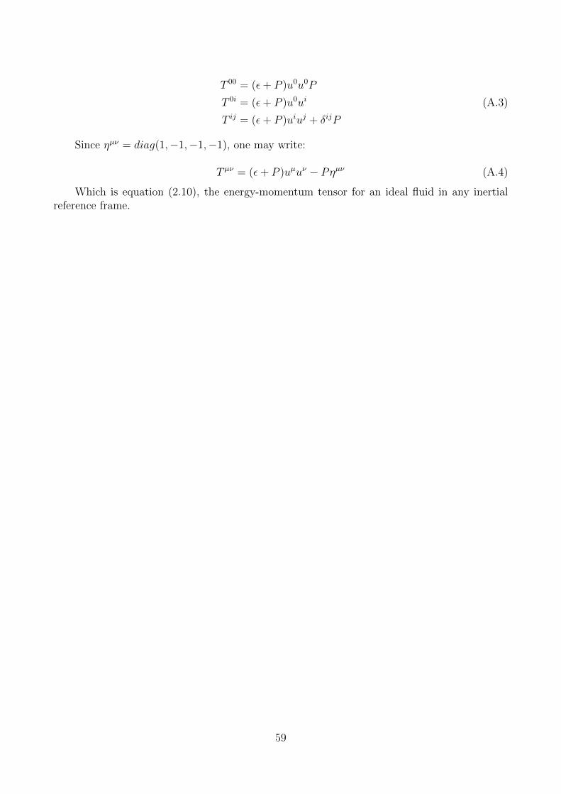
T 00 = (ε+ P )u0u0P

T 0i = (ε+ P )u0ui (A.3)

T ij = (ε+ P )uiuj + δijP

Since ηµν = diag(1,−1,−1,−1), one may write:

T µν = (ε+ P )uµuν − Pηµν (A.4)

Which is equation (2.10), the energy-momentum tensor for an ideal fluid in any inertialreference frame.

59

Appendix B

Coordinates in Heavy-Ion Collisions

The incident nuclei collide at z = t = 0 and we choose z as the collision axis. Thehydrodynamic evolution follows, starting at a proper initial time, τ0. Particles are createdaround z = t = 0 and are supposed to travel with longitudinal velocity vz = z/t. Thisprescription is boost invariant in the sense that for any Lorentz transformation along the zaxis, the relationship still holds [12, 63]. Since all particles at a given z have the same speed,vz, that is also the fluid velocity.

QGP

HG

z=tz=-t

τ0

z

t

Figure B.1: Space-time diagram of the longitudinal evolution of the collision. The black lines (z = tand z = −t) correspond to the nuclei trajectories, while the blue hyperbola represents the initialproper-time τ0. Dashed hyperbola illustrates the transition from QGP to HG and the green one is theend of the hydrodynamic expansion.

The beginning of the hydrodynamic expansion is delimited by the τ0 =√t2 − z2 hyper-

bola. As the value of proper-time changes, the stage of evolution corresponding to it will berepresented in Fig.B.1 as another hyperbola, whose equation is τ =

√t2 − z2. In addition to

proper time τ , we introduce ηs, defined as space-time rapidity:

t = τ cosh (ηs) (B.1)

z = τ sinh (ηs) (B.2)

60

When dividing (B.2) by (B.1), one should find an expression of ηs in terms of z and t.

z

t=

sinh (ηs)

cosh (ηs)= tanh (ηs)

Since tanh (ηs) = eηs−e−ηs

eηs+e−ηs:

eηs − e−ηs

eηs + e−ηs=z

t

Consequently:

z(eηs + e−ηs) = t(eηs − e−ηs)

eηs(t− z) = e−ηs(z + t)

⇒ e2ηs =

(t+ z

t− z

)Taking the natural logarithm on both sides:

ηs =1

2ln

(t+ z

t− z

)(B.3)

Under a Lorentz boost in the z direction, τ is invariant and ηs is shifted by a constant(similarly to the particle rapidity). Alongside with τ =

√t2 − z2 and Cartesian coordinates x

and y in the transverse plane, they are the variables used to depict the evolution of a heavy-ioncollision.

61

Appendix C

Relativistic Fluid’s Action in a GeneralCoordinate System

Take a general coordinate system with

ds2 = gµνdxµdxν .

Under a general transformation, x→ x′, the hypervolume element becomes

d4x′µ =

∥∥∥∥∂x′α∂xβ

∥∥∥∥ d4xµ,

where∥∥∂x′α∂xβ

∥∥ is the Jacobian(Jαβ)

determinant of the coordinate transformation[64]. Addition-ally, the metric tensor gµν may have the following expression:

gµν =∂x′α

∂xµ∂x′β

∂xνηαβ

= Jαµ Jβν ηαβ (C.1)

or, in matrix language, (gµν) = JTηJ . If g is the determinant of 4 × 4 matrix (gµν), one shallhave g = − (detJ)2 ⇒ detJ =

√−g. Hence,

d4xµ =√−gd4xµ, (C.2)

which gives the general action

I =

∫L√−gd4x, (C.3)

where L is a scalar Lagrangian density and√−gd4x is invariant.

We now proceed on presenting the covariant derivative of some contravariant vector V µ,defined as

V µ;ν ≡

∂V µ

∂xν+ ΓµναV

α, (C.4)

from which we may derive the divergence, V µ;µ:

V µ;µ = ∂νV

µ + ΓµµαVα. (C.5)

62

The coefficients Γµνα are known as components of the affine connection or as Christoffel symbolsand can be written in terms of the metric tensor:

Γµνα =1

2gσµ[∂gασ∂xν

+∂gνσ∂xα

− ∂gαν∂xσ

], (C.6)

where

Γµµα =1

2gσµ [∂µgασ + ∂αgµσ − ∂σgαµ]

=1

2gσµ∂αgµσ.

Knowing that Tr [M−1∂λM ] = ∂λ [ln (detM)] for an arbitrary matrix M ,

Γµµα =1

2∂α ln g =

1√−g

∂α√−g. (C.7)

Substituting the previous expression in (C.5) shall yield:

V µ;µ = ∂νV

µ +1√−g

∂α(√−g)V α

=1√−g

∂α(√−gV α

). (C.8)

The Lagrangian for a relativistic fluid in motion can be taken as L = −E[65], where E isthe fluid’s rest energy. Using (C.3) and L =

∫d3xL yields the action

I = −∫d4x√−gε, (C.9)

where ε is the density distribution associated to E, such that E =∫d3xε. From (C.8), we have

the general forms for the constraints ∂µ(suµ) = 0 and ∂µ(nuµ) = 0 presented in Section 2.1:

(suµ);µ =1√−g

∂µ(√−gsuµ

)= 0, (C.10)

(nuµ);µ =1√−g

∂µ(√−gnuµ

)= 0. (C.11)

63

References

[1] CERN Press Release Feb. 10, (2000) http://press-archive.web.cern.ch/press-rchive/PressReleases/Releases2000/PR01.00EQuarkGluonMatter.html;

[2] Brookhaven National Laboratory, Hunting the Quark Gluon Plasma (QGP) Formal Report- Results from the first 3 years at RHIC, Assessments by the experimental collaborations(2005);

[3] E. Fermi, Prog. Theor. Phys. 5, 570 (1950);

[4] L. D. Landau, Izv. Akad. Nauk. SSSR Ser. Fiz. 17, 51 (1953);

[5] S. Z. Belenkij, and L. D. Landau, Usp. Fiz. Nauk 56, 309 (1955), from “Collected papersof L. D. Landau” (ed. D. Ter-Haar, Pergamon, Oxford, 1965) p. 665;

[6] H. J. Drescher, F.M. Liu, S. Ostapchenko, T. Pierog, and K. Werner, Phys. Rev. C 65,054902 (2002);

[7] C. E. Aguiar, T. Kodama, T. Osada, and Y. Hama, J. Phys. G 27, 75 (2001);

[8] T. Kodama, C. E. Aguiar, T. Osada, and Y. Hama, J. Phys. G: Nucl. Part. Phys. 27 (2001)557-560;

[9] P. Kovtun, J. Phys. A: Math. Theor. 45 (2012) 473001 [arXiv:hep-th/1205.5040];

[10] L. D. Landau, and E. M. Lifshitz, Fluid Mechanics, ed. Pergamon Press (1987);

[11] Lecture notes from the course Fluidos Dissipativos Relativısticos e suas Recentes Aplicacoesem Fısica de Altas Energias - PGF5293-1/1, Prof. Jorge Noronha (2013);

[12] J.-Y. Ollitrault, Eur.J.Phys. 29: 275-302 (2008) [arXiv:nucl-th/0708.2433];

[13] S. Weinberg, Gravitation and Cosmology: Principles and Applications of the General The-ory of Relativity, ed. John Wiley & Sons, Inc. (1972);

[14] W. Florkowski, Phenomenology of Ultra-Relativistic Heavy-Ion Collisions, ed. World Sci-entific (2010);

[15] S. Jeon, and U. Heinz, [arXiv:hep-ph/1503.03931] (2015);

[16] Y. Hama, T. Kodama, and O. Socolowski Jr., Brazilian Journal of Physics, vol. 35, no.1,p. 24 (2005);

[17] B. Alver, and G. Roland, Phys.Rev. C 81, 054905 (2010) [arXiv:nucl-th/1003.0194];

64

[18] B. Alver, C. Gombeaud, M. Luzum, and J.-Y. Ollitrault, Phys.Rev. C 82, 034913 (2010)[arXiv:nucl-th/1007.5469];

[19] C. Gale, S. Jeon, B. Schenke, P. Tribedy, and R. Venugopalan, [arXiv:hep-ph/1210.5144](2012);

[20] B. Schenke, and R. Venugopalan, Phys. Rev. Lett. 113, 102301 (2014) [arXiv:nucl-th/1405.3605];

[21] G. Denicol, C. Gale, S. Jeon, J.-F. Paquet, and B. Schenke, [arXiv:nucl-th/1406.7792](2014);

[22] C. Shen, Z. Qiu, and U. Heinz, Phys. Rev. C 92, 014901 (2015) [arXiv:nucl-th/1502.04636];

[23] F. Gardim, F. Grassi, M. Luzum, and J.-Y. Ollitrault, Phys. Rev. C 87, 031901(R) (2013)[arXiv:nucl-th/1211.0989];

[24] J. Takahashi et al., Phys. Rev. Lett. 103, 242301 (2009);

[25] R. Andrade, F. Grassi, Y. Hama, W.-L. Qian, Physics Letters B, v. 712, p. 226-230, (2012)[arXiv:nucl-th/1008.4612];

[26] Y. Hama, R. P. G. Andrade, F. Grassi, O. Socolowsky Jr., T. Kodama, B. Tavares, andS. S. Padula, Nucl.Phys. A 774, 169 (2006);

[27] P. Huovinen, P. Petreczky, Nucl.Phys. A 837, 26 (2010) [arXiv:hep-ph/0912.2541];

[28] E. Megıas, E. R. Arriola, and L. L. Salcedo, Nucl. Phys. Proc. Suppl. 234, 313-316 (2013)[arXiv:hep-ph/1207.7287];

[29] S. R. A. Salinas, Introduction to Statistical Physics, ed. Springer (2001);

[30] A. Chodos, R. L. Jaffe, K. Johnson, C. B. Thorn, and V. F. Weisskopf, Phys. Rev. D 9,3471-95 (1974);

[31] A. Chodos, R. L. Jaffe, K. Johnson, and C. B. Thorn, Phys. Rev. D 10, 2599 (1974);

[32] Z. Fodor and S. D. Katz, JHEP 0203, 014 (2002) [arXiv:hep-lat/0106002];

[33] J. Casalderrey-Solana, H. Liu, D. Mateos, K. Rajagopal, and U. A. Wiedemann,[arXiv:hep-th/1101.0618] (2012);

[34] K. Rajagopal, and F. Wilczek, [arXiv:hep-ph/0011333] (2000);

[35] P. Petreczky, Nucl. Phys. A 830, 11c-18c (2009) [arXiv:hep-ph/0908.1917];

[36] P. Huovinen, P. Petreczky, and C. Schmidt, [arXiv:nucl-th/1407.8532] (2014);

[37] F. Cooper, and G. Frye, Phys. Rev. D 10, 186 (1974);

[38] F. Debbasch, J.P. Rivet, and W.A. van Leeuwen, Physica A 301, 181 (2001) [arXiv:astro-ph/0707.2499];

[39] D. H. Rischke, [arXiv:nucl-th/9809044] (1998);

65

[40] PhD Thesis: Sobre a evolucao hidrodinamica da materia nuclear criada em colisoes deıons pesados relativısticos - um estudo com condicoes iniciais flutuantes, Universidade deSao Paulo (2011), R. P. G. Andrade;

[41] L. B. Lucy, Astrophys. J. 82, 1013 (1977);

[42] R. A. Gingold and J. J. Monaghan, Mon. Not. R. Astro. Soc. 181, 375 (1977);

[43] J. Noronha-Hostler, J. Noronha, and F. Grassi, Phys. Rev. C 90, 034907 (2014);

[44] C. Aguiar, T. Kodama, Y. Hama, and T. Osada, Nucl. Phys. A 698 (2002) 639c,[arXiv:nucl-th/0102011];

[45] ALICE Collaboration, Phys. Rev. C 88, 044909 (2013) [arXiv:nucl-ex/1301.4361];

[46] ALICE Collaboration, Phys. Lett. B 726, 610-622 (2013) [arXiv:nucl-ex/1304.0347];

[47] ALICE Collaboration, Phys. Lett. B 720, 52-62 (2013) [arXiv:hep-ex/1208.2711];

[48] J.-Y. Ollitrault, Phys. Rev. D 46, 229 (1991);

[49] A. M. Poskanzer, and S. A. Voloshin, Phys. Rev. C 58, 1671 (1998) [arXiv:nucl-ex/9805001];

[50] F. G. Gardim, F. Grassi, Y. Hama, M. Luzum, and J.-Y. Ollitrault, Phys. Rev. C 83,064901 (2011) [atXiv:nucl-th/1103.4605];

[51] CMS Collaboration, Phys. Rev. C 87, 014902 (2013) [arXiv:nucl-ex/1204.1409];

[52] CMS Collaboration, Phys. Rev. C 89, 044906 (2014) [arXiv:nucl-ex/1310.8651];

[53] ATLAS Collaboration, JHEP 11, 183 (2013) [arXiv:hep-ex/1305.2942];

[54] J. Noronha-Hostler, G. S. Denicol, J. Noronha, R. P. G. Andrade, and F. Grassi, Phys.Rev. C 88, 044916 (2013) [arXiv: nucl-th/1305.1981] (2013);

[55] N. Borghini, P. M. Dinh, and J.-Y. Ollitrault, Phys. Rev. C 64, 054901 (2001) [arXiv:nucl-th/010540];

[56] R. S. Bhalerao, N. Borghini,and J.-Y. Ollitrault, Nucl. Phys. A 727, 373 (2003);

[57] N. Borghini, R. S. Bhalerao, and J.-Y. Ollitrault, J. of Phys. G 30, S1213 (2004);

[58] C. Gale, S. Jeon, B. Schencke, P. Tribedy, and R. Venugopalan, [arXiv: nucl-th/1209.6330](2012);

[59] B. B. Back et al., Braz. J. Phys. 34, 829 (2004);

[60] PhD thesis: Efeitos da equacao de estado em hidrodinamica relativıstica atraves de algunsobservaveis, Instituto de Fısica Teorica - Universidade Estadual Paulista (2014), D. M.Dudek;

[61] B. B. Back et al.[PHOBOS Collaboration], Phys. Rev. B 578, 297 (2004);

[62] F. G. Gardim, F. Grassi, M. Luzum, and J.-Y. Ollitrault, Phys. Rev. Lett. 109, 202302(2012) [arXiv:nucl-th/1203.2882];

66

[63] J. D. Bjorken, Phys. Rev. D 27, 140 (1983);

[64] J. A. Peacock, Cosmological Physics, Cambridge University Press (1999);

[65] H. T. Elze, Y. Hama, T. Kodama, M. Makler, and J. Rafelski, [arXiv:hep-ph/9809570](1998);

67