Hierarchical Linear Models: Applications in Educational ...hkier.fed.cuhk.edu.hk/journal/wp-content/uploads/2011/10/erj_v26n1... · Hierarchical Linear Models 43 The Necessity for

Educational Research Journal《教育研究學報》, Vol. 26, No. 1, Summer 2011 © Hong Kong Educational Research Association 2011

Hierarchical Linear Models: Applications in Educational Assessment Research Hussain Alkharusi Sultan Qaboos University, Oman

Of increasing interest to the educational assessment researchers is the role of educational assessment practices on student achievement-related outcomes (Black & Wiliam, 1998). By their inherent nature, the data collected in this line of research are hierarchically structured in that students are nested within classes. As might be expected, not considering the nested nature of the data in the educational assessment research may lead to invalid inferences about the relationship between educational assessment and student motivation and achievement. As a means of drawing valid inferences from hierarchically structured data, this paper highlights the utility and applicability of hierarchical linear modeling techniques in the educational assessment research. These techniques not only facilitate a decomposition of the relationship between the variables into separate student-level and class-level components, but also recognize the dependence among the outcomes of students within the same class (Raudenbush & Bryk, 2002). This dependence may arise as a result of shared students’ experiences with regard to the teacher’s assessment practices. This paper discusses the necessity for using these techniques in

________________________ Correspondence concerning this article should be addressed to Hussain Alkharusi, Department of Psychology, College of Education, P. O. Box 32 A1-Khod P.C.: 123, Sultanate of Oman. E-mail: [email protected]

42 Hussain Alkharusi

the educational assessment research in order to validate inferences and further research agenda in this area.

Key words: Hierarchical Linear Models, educational assessment research, data analysis

Introduction

Of increasing interest to educational assessment researchers is the influence of educational assessment practices on student motivation and achievement (Brookhart, 1994). In this line of research, key explanatory variables are typically measured at the classroom-level whereas the outcome variables are at the student-level. Under these circumstances, the researchers are required to utilize hierarchical linear modeling (HLM) analyses (Raudenbush & Bryk, 2002) to not only appropriately test relationships occurring at each level of the hierarchy, but also estimate potentially meaningful relationships that might cross the different levels of the hierarchy.

Given the movement in educational assessment research toward the role of educational assessment practices on student outcomes, it seems reasonable to argue that careful consideration of the hierarchical structure of the data is certainly warranted. The purpose of this paper is to highlight the utility and applicability of HLM as an appropriate way of handling the hierarchical structure of the data collected in educational assessment research. It should be acknowledged that the paper is an expository summary of HLM which is originated from Raudenbush and other statisticians. The readers are encouraged to utilize the references cited in the paper for more details about the topic. The paper begins with a discussion of the necessity for using HLM in the educational assessment research and then provides an overview of the conceptual framework of HLM along with certain methodological issues that need to be considered when employing the HLM. Throughout the paper, a real example from educational assessment literature will be used to illustrate the points.

Hierarchical Linear Models 43

The Necessity for HLM

HLM is a statistical method for analyzing hierarchically structured data (Raudenbush & Bryk, 2002). We say that a data set is hierarchically structured when we have lower-level observations nested within higher-level observations. For example, educational assessment researchers seeking to examine the effects of classroom assessment practices on student achievement may collect data on students in classrooms. Such data may include variables that describe students, such as student socioeconomic status (SES) and student achievement, as well as variables that describe classrooms, such as teacher’s frequent use of alternative assessments (ALTR). By their nature, such data require an analysis that takes into account the variability associated with each level of the hierarchy, that is, the variability within-classrooms and the variability between-classrooms.

The need for using HLM originates from the problems of using single-level analyses for hierarchically structured data. Some of these problems are aggregation bias, fallacy of wrong level, and unit of analysis. First, when data are aggregated, the within-class variance would be ignored and as such much information is lost, statistical power is reduced, a shift occurs in the meaning of the variables, and the relationship between the variables might differ in magnitude and direction for different levels of the analysis (Hox, 2002; Kreft & Leeuw, 1998; Snijders & Bosker, 1999). Likewise, when data are disaggregated, we might violate the assumption of independent observations which can lead to smaller estimates of standard errors that can result in rejecting the null hypotheses more often than we should (Hox, 2002; Kreft & Leeuw, 1998; Raudenbush & Bryk, 2002). Students within a classroom may share common characteristics of the teacher and his or her assessment practices, and as such even though students respond differently to the same classroom assessment activity, their responses may have commonality. As a result, outcome observations on students cannot often be assumed independent. Aggregation or disaggregation of the data can also lead to fallacies of the wrong level in which


conclusions are made at one level based on analyses at another level (Hox, 2002; Kreft & Leeuw, 1998; Snijders & Bosker, 1999).

Moreover, the appropriate unit of analysis, students or classrooms, may become a problematic issue in single-level analyses when the explanatory variables are measured at the classroom-level, but the outcome variable is measured at the student-level (Raudenbush & Bryk, 2002). For example, if a researcher is concerned with how class-level variables (e.g., teacher’s frequent uses of ALTR) affect the student-level outcome (e.g., student achievement), the question then arises as to what are the objects of measurement and analysis in the study and how to deal with potentially meaningful relations that might cross the class-level and student-level. As might be expected, ignoring the hierarchical nested nature of the data can result in misguided conclusions about the impact of classroom assessment on student. Fortunately, HLM acknowledges both levels of the hierarchy as critically important and as such treats them simultaneously (Kreft & Leeuw, 1998).

A Conceptual Illustration of HLM

To understand how HLM operates, let’s suppose that a researcher is interested in how student’s SES and teacher’s frequent use of ALTR influence student achievement. The researcher has collected data about teachers’ self-reported frequency of using ALTR and students’ SES and achievement scores. In this example, the objects of interest and measurement are teachers and students. Under the HLM framework, a clear conceptual distinction is made between student-level and class-level variables and effects. This conception is reflected in the two models that make up a two-level HLM. The first model captures the primary effects at the student-level within each class. The second model attempts to explain these student-level effects in terms of class-level variables.


A Fully Unconditional Model

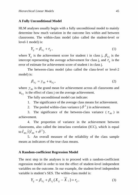
HLM analyses usually begin with a fully unconditional model to mainly determine how much variation in the outcome lies within and between classrooms. The within-class model (also called the student-level or level-1 model) is:

ijjij rY += 0β , (1)

where is the achievement score for student i in class j, ijY j0β is the intercept representing the average achievement for class j, and is the error of estimate for achievement score of student i in class j.

ijr

The between-class model (also called the class-level or level-2 model) is:

,0000 jj u+= γβ (2)

where 00γ is the grand mean for achievement across all classrooms and is the effect of class j on the average achievement. ju0

The fully unconditional model can indicate: 1. The significance of the average class means for achievement. 2. The pooled within-class variance ( ) in achievement. 2σ̂3. The significance of the between-class variance ( 00τ ) in

achievement. 4. The proportion of variance in the achievement between

classrooms, also called the intraclass correlation (ICC), which is equal to )ˆˆ(ˆ 2

0000 σττ + . 5. An overall measure of the reliability of the class sample

means as indicators of the true class means.

A Random-coefficient Regression Model

The next step in the analyses is to proceed with a random-coefficient regression model in order to test the effect of student-level independent variables on the outcome. In our example, the student-level independent variable is student’s SES. The within-class model is:

ijjijjjij rXXY +−+= )( .10 ββ , (3)


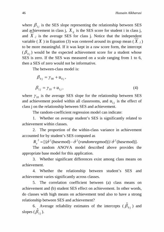
where j1β is the SES slope representing the relationship between SES and achievement in class j, is the SES score for student i in class j, and

ijXjX . is the average SES for class j. Notice that the independent

variable ( X ) in Equation (3) was centered around its group mean ( jX . ) to be more meaningful. If it was kept in a raw score form, the intercept ( j0β ) would be the expected achievement score for a student whose SES is zero. If the SES was measured on a scale ranging from 1 to 6, then a SES of zero would not be informative.

The between-class model is:

jj u0000 += γβ ,

jj u1101 += γβ , (4)

where 10γ is the average SES slope for the relationship between SES and achievement pooled within all classrooms, and is the effect of class j on the relationship between SES and achievement.

ju1

The random-coefficient regression model can indicate: 1. Whether on average student’s SES is significantly related to

achievement within classes. 2. The proportion of the within-class variance in achievement

accounted for by student’s SES computed as mod)](ˆ/mod)}(ˆmod)(ˆ[{ 2222 baserandomregbaseRy σσσ −= .

The random ANOVA model described above provides the appropriate base model for this application.

3. Whether significant differences exist among class means on achievement.

4. Whether the relationship between student’s SES and achievement varies significantly across classes.

5. The correlation coefficient between (a) class means on achievement and (b) student SES effect on achievement. In other words, do classes with high means on achievement tend also to have a strong relationship between SES and achievement?

6. Average reliability estimates of the intercepts ( ) and slopes ( ).

j0β̂j1β̂


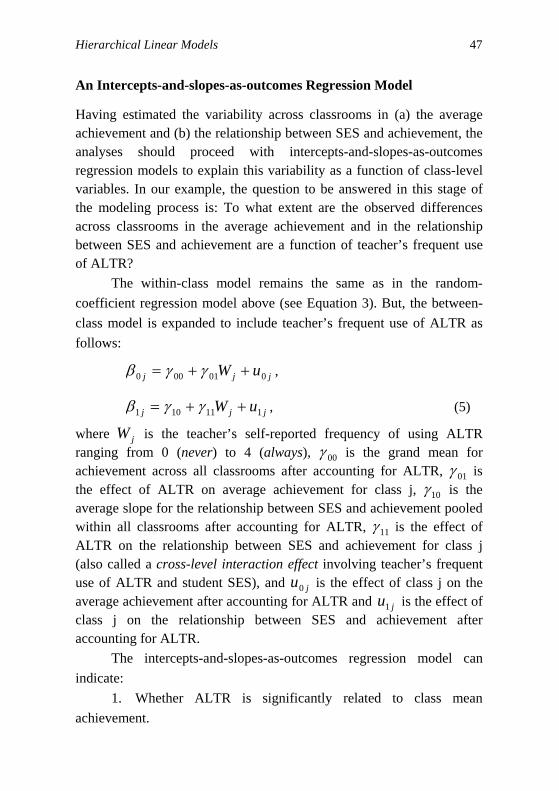
An Intercepts-and-slopes-as-outcomes Regression Model

Having estimated the variability across classrooms in (a) the average achievement and (b) the relationship between SES and achievement, the analyses should proceed with intercepts-and-slopes-as-outcomes regression models to explain this variability as a function of class-level variables. In our example, the question to be answered in this stage of the modeling process is: To what extent are the observed differences across classrooms in the average achievement and in the relationship between SES and achievement are a function of teacher’s frequent use of ALTR?

The within-class model remains the same as in the random-coefficient regression model above (see Equation 3). But, the between-class model is expanded to include teacher’s frequent use of ALTR as follows:

jjj uW 001000 ++= γγβ ,

jjj uW 111101 ++= γγβ , (5)

where is the teacher’s self-reported frequency of using ALTR ranging from 0 (never) to 4 (always),

jW00γ is the grand mean for

achievement across all classrooms after accounting for ALTR, 01γ is the effect of ALTR on average achievement for class j, 10γ is the average slope for the relationship between SES and achievement pooled within all classrooms after accounting for ALTR, 11γ is the effect of ALTR on the relationship between SES and achievement for class j (also called a cross-level interaction effect involving teacher’s frequent use of ALTR and student SES), and is the effect of class j on the average achievement after accounting for ALTR and is the effect of class j on the relationship between SES and achievement after accounting for ALTR.

ju0

ju1

The intercepts-and-slopes-as-outcomes regression model can indicate:

1. Whether ALTR is significantly related to class mean achievement.


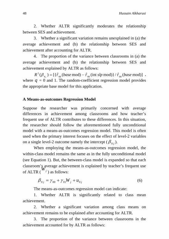
2. Whether ALTR significantly moderates the relationship between SES and achievement.

3. Whether a significant variation remains unexplained in (a) the average achievement and (b) the relationship between SES and achievement after accounting for ALTR.

4. The proportion of the variance between classrooms in (a) the average achievement and (b) the relationship between SES and achievement explained by ALTR as follows:

mod)](ˆ/mod)}(intˆmod)(ˆ[{)(2 baseslpbaseR qqqqqqq jτττβ −= ,

where q = 0 and 1. The random-coefficient regression model provides the appropriate base model for this application.

A Means-as-outcomes Regression Model

Suppose the researcher was primarily concerned with average differences in achievement among classrooms and how teacher’s frequent use of ALTR contributes to these differences. In this situation, the researcher should follow the aforementioned fully unconditional model with a means-as-outcomes regression model. This model is often used when the primary interest focuses on the effect of level-2 variables on a single level-2 outcome namely the intercept ( j0β ).

When employing the means-as-outcomes regression model, the within-class model remains the same as in the fully unconditional model (see Equation 1). But, the between-class model is expanded so that each classroom’s average achievement is explained by teacher’s frequent use of ALTR ( ) as follows: jW

jjj uW 001000 ++= γγβ (6)

The means-as-outcomes regression model can indicate: 1. Whether ALTR is significantly related to class mean

achievement. 2. Whether a significant variation among class means on

achievement remains to be explained after accounting for ALTR. 3. The proportion of the variance between classrooms in the

achievement accounted for by ALTR as follows:


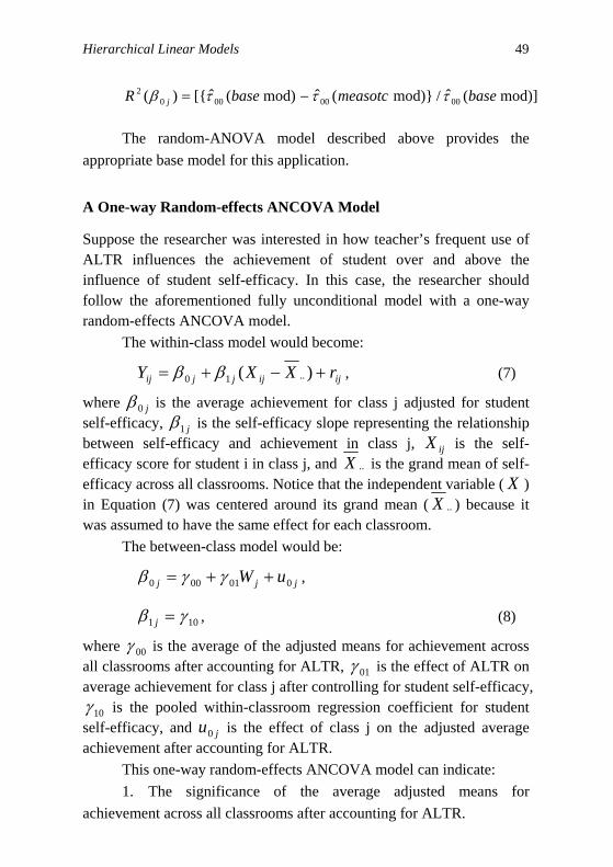
mod)](ˆ/mod)}(ˆmod)(ˆ[{)( 00000002 basemeasotcbaseR j τττβ −=

The random-ANOVA model described above provides the

appropriate base model for this application.

A One-way Random-effects ANCOVA Model

Suppose the researcher was interested in how teacher’s frequent use of ALTR influences the achievement of student over and above the influence of student self-efficacy. In this case, the researcher should follow the aforementioned fully unconditional model with a one-way random-effects ANCOVA model.

The within-class model would become:

ijijjjij rXXY +−+= )( ..10 ββ , (7)

where j0β is the average achievement for class j adjusted for student self-efficacy, j1β is the self-efficacy slope representing the relationship between self-efficacy and achievement in class j, is the self-efficacy score for student i in class j, and

ijX..X is the grand mean of self-

efficacy across all classrooms. Notice that the independent variable ( X ) in Equation (7) was centered around its grand mean ( ..X ) because it was assumed to have the same effect for each classroom.

The between-class model would be:

jjj uW 001000 ++= γγβ ,

101 γβ =j , (8)

where 00γ is the average of the adjusted means for achievement across all classrooms after accounting for ALTR, 01γ is the effect of ALTR on average achievement for class j after controlling for student self-efficacy,

10γ is the pooled within-classroom regression coefficient for student self-efficacy, and is the effect of class j on the adjusted average achievement after accounting for ALTR.

ju0

This one-way random-effects ANCOVA model can indicate: 1. The significance of the average adjusted means for

achievement across all classrooms after accounting for ALTR.


2. Whether ALTR is significantly related to class mean achievement after controlling for student self-efficacy.

3. The significance of the average effect of student self-efficacy on student achievement across all classrooms.

4. The proportion of the within-class variance in achievement accounted for by student self-efficacy computed as

mod)](ˆ/mod)}cov(ˆmod)(ˆ[{ 2222 baserandomanbaseR y σσσ −=

The random ANOVA model described above provides the appropriate base model for this application.

5. Whether a significant variation in the adjusted average achievement remains unexplained after accounting for ALTR.

6. The proportion of the variance in the adjusted class average achievement accounted for by ALTR as follows:

mod)](ˆ/mod)}cov(ˆmod)(ˆ[{)( 00000002 baserandomanbaseR j τττβ −=

The random-ANOVA model described above provides the

appropriate base model for this application. When compared to the classical ANCOVA approach, the HLM

approach is more advantageous for the following four reasons (Kreft & Leeuw, 1998; Raudenbush & Bryk, 2002):

1. In HLM, the variability among outcome adjusted classrooms’ means can be explained by classroom characteristics, whereas the classical ANCOVA approach may not be able to state why do the classrooms differ in their adjusted outcome means.

2. In the classical ANCOVA approach, we cannot partition the random part as we do in the HLM approach into within- and between-class variability.

3. The classical ANCOVA approach assumes that the effect of the covariate on the outcome is assumed to be the same across all the groups in the population, whereas in the HLM approach, this assumption becomes less strict by building a model to explain variability in the slopes if the effect of the level-1 covariate is found to vary across level-2 units.


4. The HLM approach provides more efficient estimates of the class-level effects than the classical ANCOVA approach when classrooms have unequal number of students.

Some Methodological Issues in HLM

Assumptions

The validity of inferences based on the two-level HLM considered in our example can be assessed by verifying the tenability of six key assumptions (Raudenbush & Bryk, 2002):

1. Level-1 errors are independent and identically normally distributed with a mean of 0 and a variance of . The normality assumption can be checked by looking at a normal probability plot for the standardized level-1 residuals pooled across units. These residuals should be approximately on a 45 degree line. The homogeneity of variance assumption can be checked by running a test for homogeneity of level-1 variances provided by HLM6 program (Raudenbush, Bryk, Cheong, & Congdon, 2004). A non-statistically significant provides evidence of the level-1 variance homogeneity.

2σ

2χ

2χ2. The level-1 predictor is independent of level-1 errors. This

assumption can be checked by plotting level-1 residuals against predicted values of the student-level outcome. The lack of relationship signals a proper model specification at the student-level and hence meeting this assumption.

3. Level-2 errors and are bivariate normal, each with a mean of 0, variances of

ju0 ju1

00τ and 11τ , respectively, and a covariance of 01τ . This assumption can be checked by inspecting a Q-Q plot of the Mahalanobis distances. If the Q-Q plot looks approximately like a 45 degree line, then the assumption of bivariate normality is tenable.

4. The level-2 predictor is independent of level-2 errors. This assumption can be checked by plotting the empirical Bayes (EB) estimates of level-2 residuals against the predicted values of the


corresponding level-1 coefficient. The lack of relationships signals an adequate model specification at the class-level.

5. Level-1 errors are independent of level-2 errors. This assumption can be checked by inspecting a scatter plot of the Mahalanobis distances for the level-2 residuals against the level-1 residuals. A null correlation between the residuals from both levels provides evidence for the tenability of this assumption.

6. Predictors at each level are not correlated with random parts at the other level. This assumption is met by having null relationships when (a) plotting the Mahalanobis distances for the level-2 residuals against the predicted values of level-1 model and (b) plotting the level-1 residuals against the predicted values of each level-1 coefficient based on level-2 model.

Modeling Level-1 Coefficients

Each level-1 coefficient qjβ , where q = 0, 1, …, Q coefficients and j = 1, 2, …, J level-2 units; defined in level-1 model can be modeled at level-2 as one of three general forms (Raudenbush & Bryk, 2002):

1. A fixed level-1 coefficient denoted by 0qqj γβ = . In this form, level-2 predictors are assumed to have no effect on qjβ .

2. A random level-1 coefficient denoted either by

qjqqj u+= 0γβ or , where s = 1, 2, …, S level-2 predictors. In

qj

S

ssjqsqqj uW ++= ∑

=10 γγβ

qjqqj u+= 0γβ , the level-1 coefficients are assumed to vary randomly over the population level-2 units. In

sqj

S

sjqsqqj uW ++= ∑=

0 γγβ1

, the level-1 coefficients are assumed to have both a non-random variation explained by level-2 predictors and a random variation that remains unexplained.

3. A non-randomly varying level-1 coefficient denoted by ∑+=

S

=sjqsqqj W0 γγβ

s 1. In this form, the level-1 coefficients do vary

across the population of level-2 units as a function of level-2 predictors, but not as random.


The modeling of level-1 coefficients depends on the following indices (Raudenbush & Bryk, 2002):

1. The point estimate of the variance for the level-1 coefficient , in that, as qqqj τβ ˆ)ˆvar( = qqτ̂ becomes negligible, its corresponding level-1 coefficient may be specified as fixed.

2. The homogeneity test of H0: 2χ 0=qqτ , in that, as the H0

becomes tenable, its corresponding level-1 coefficient may be specified as fixed.

3. The likelihood ratio test (i.e., deviance) of the variance-covariance components, in that, two models with the same fixed parts (i.e., the gammas s'γ ) are compared. The first unrestricted model includes the variance components of the level-1 coefficient under question. The second restricted model constrains these components to zero. If there is no significant difference between the deviances of the two models, then the restricted model is preferred and the level-1 coefficient of interest may be specified as fixed.

4. The reliability of because it indicates the potentially explainable variation in the estimated

qjβ̂qjβ . A small amount of reliability

(e.g., less than .05) suggests the need to specify the corresponding level-1 coefficient as fixed because there is not much variability in that coefficient to be explained by level-2 explanatory variables.

5. The correlations among qjβ , in that, as the correlations are high (e.g., higher than .70), one or more of the level-1 coefficients may be specified as fixed.

6. The theory underlying the research, in that, one or more of the above five statistical indices may indicate no random variation, but the research theory may suggest that the corresponding level-1 coefficient varies across level-2 units as a function of level-2 variables. In this case, that coefficient may need to be specified as non-randomly varying.


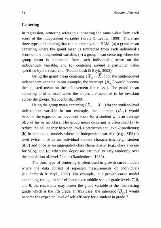
Centering

In regression, centering refers to subtracting the same value from each score of the independent variables (Kreft & Leeuw, 1998). There are three types of centering that can be employed in HLM: (a) a grand mean centering where the grand mean is subtracted from each individual’s score on the independent variable, (b) a group mean centering where the group mean is subtracted from each individual’s score on the independent variable, and (c) centering around a particular value specified by the researcher (Raudenbush & Bryk, 2002).

Using the grand mean centering )( ..XX ij − for the student-level independent variable in our example, the intercept )( 0 jβ would become the adjusted mean on the achievement for class j. The grand mean centering is often used when the slopes are assumed to be invariant across the groups (Raudenbush, 1989).

Using the group mean centering )( . jij XX − for the student-level independent variable in our example, the intercept )( 0 jβ would become the expected achievement score for a student with an average SES of his or her class. The group mean centering is often used (a) to reduce the collinearity between level-1 predictors and level-2 predictors; (b) in contextual models where an independent variable (e.g., SES) is used twice, once as an individual student characteristic (e.g., student SES) and once as an aggregated class characteristic (e.g., class average for SES); and (c) when the slopes are assumed to vary randomly over the population of level-2 units (Raudenbush, 1989).

The third type of centering is often used in growth curve models where the data consist of repeated measurements on individuals (Raudenbush & Bryk, 2002). For example, in a growth curve model examining change in self-efficacy over middle school grade levels 7, 8, and 9, the researcher may center the grade variable at the first testing grade which is the 7th grade. In this case, the intercept )( 0 jβ would become the expected level of self-efficacy for a student in grade 7.


Sample Size

There are two sorts of sample size that need to be considered in research designs involving a two-level hierarchically structured data. These are the sample size of level-1 units (e.g., students) within each level-2 unit (n) (e.g., classrooms) and the sample size of the level-2 units (J), with

being the total sample size for the level-1 units (Snijders & Bosker, 1999). Although a number of software programs have been designed for calculations of power (e.g., Raudenbush & Liu, 2000; Snijders & Bosker, 1993), there are no specific guidelines regarding appropriate sample sizes for hierarchical linear models. Yet, some general recommendations have been discussed. For example, Mok (1995) indicated that less bias and more efficiency would be expected from research designs involving more classrooms and fewer students per classroom than designs involving fewer classrooms and more students per classroom. After reviewing some simulation studies investigating the power of HLM, Kreft and Leeuw (1998) indicated that 60 classrooms with 25 students per classroom, bringing the total number to 1,500, will produce a sufficiently high power. Bassiri (1988) as well as van der Leeden and Busing (1994) showed that at least 30 classrooms and 30 students within each classroom are needed to obtain a sufficient power (e.g., .90) to detect interactions between variables measured at different levels in hierarchically structured data (i.e., cross-level interactions).

)( nJ ×

An Empirical Example: Effects of Assessment Practices on Students’ Performance Goals

Alkharusi (2008) used HLM to examine the effects of classroom assessment practices on students’ performance goal orientation. The data were drawn from a sample of 1,636 students and their corresponding 83 teachers from public ninth grade science classes in Oman, with an average of 20 students per class. This paper presents some of the analysis and discusses the logic involved in each step. Four research questions were attempted to be answered:


1. Do ninth grade science classrooms in Oman vary in performance goals (GOAL)?

2. What are some of the student characteristics that might have effects on GOAL?

3. Do the effects of student characteristics on GOAL vary across classrooms?

4. What are some of the classroom characteristics that might help explain the variability in the GOAL and in the effects of student characteristics on GOAL across classrooms?

The purpose of these research questions was to construct a

parsimonious model explaining student’s performance goal orientation as a function of student-level and class-level characteristics. The data pertaining to these questions were hierarchically structured, in that students were nested within classes. Therefore, HLM analysis was conducted. All variables, except for class’s gender which was a dummy variable (1 = female classes and –1 = male classes), were standardized to a mean of zero and a standard deviation of one. The student-level independent variables were group-mean centered. The variables were as follows:

The Dependent Variable

- Student’s performance goal orientation (GOAL)

Independent Variables at the Student-level

- Student’s self-efficacy (SEFC) - Student’s perceptions of the assessment environment as being learning-oriented (SLA) - Student’s perceptions of the assessment environment as being harsh-oriented (SHA) - Student’s perceptions of the assessment environment as being public-oriented (SPA)


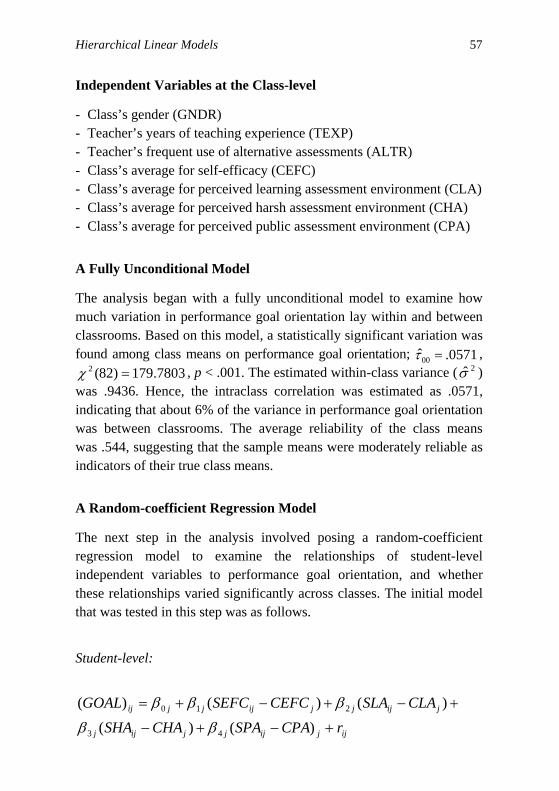
Independent Variables at the Class-level

- Class’s gender (GNDR) - Teacher’s years of teaching experience (TEXP) - Teacher’s frequent use of alternative assessments (ALTR) - Class’s average for self-efficacy (CEFC) - Class’s average for perceived learning assessment environment (CLA) - Class’s average for perceived harsh assessment environment (CHA) - Class’s average for perceived public assessment environment (CPA)

A Fully Unconditional Model

The analysis began with a fully unconditional model to examine how much variation in performance goal orientation lay within and between classrooms. Based on this model, a statistically significant variation was found among class means on performance goal orientation; 0571.ˆ00 =τ ,

, p < .001. The estimated within-class variance ( ) was .9436. Hence, the intraclass correlation was estimated as .0571, indicating that about 6% of the variance in performance goal orientation was between classrooms. The average reliability of the class means was .544, suggesting that the sample means were moderately reliable as indicators of their true class means.

7803.179)82(2 =χ 2σ̂

A Random-coefficient Regression Model

The next step in the analysis involved posing a random-coefficient regression model to examine the relationships of student-level independent variables to performance goal orientation, and whether these relationships varied significantly across classes. The initial model that was tested in this step was as follows.

Student-level:

ijjijjjijj

jijjjijjjij

rCPASPACHASHA

CLASLACEFCSEFCGOAL

+−+−

+−+−+=

)()(

)()()(

43

210

ββ

βββ


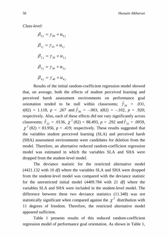
Class-level:

jj u0000 += γβ

jj u1101 += γβ

jj u2202 += γβ

jj u3303 += γβ

jj u4404 += γβ

Results of the initial random-coefficient regression model showed that, on average, both the effects of student perceived learning and perceived harsh assessment environments on performance goal orientation tended to be null within classrooms; 20γ̂ = .031, t(82) = 1.118, p = .267 and 30γ̂ = –.003, t(82) = –.102, p = .920; respectively. Also, each of these effects did not vary significantly across classrooms; 22τ̂ = .0136, (82) = 88.493, p = .292 and2χ 33τ̂ = .0059,

(82) = 83.956, p = .419; respectively. These results suggested that the variables student perceived learning (SLA) and perceived harsh (SHA) assessment environments were candidates for deletion from the model. Therefore, an alternative reduced random-coefficient regression model was estimated in which the variables SLA and SHA were dropped from the student-level model.

2χ

The deviance statistic for the restricted alternative model (4421.132 with 10 df) where the variables SLA and SHA were dropped from the student-level model was compared with the deviance statistic for the unrestricted initial model (4409.784 with 21 df) where the variables SLA and SHA were included in the student-level model. The difference between these two deviance statistics (11.348) was not statistically significant when compared against the distribution with 11 degrees of freedom. Therefore, the restricted alternative model appeared sufficient.

2χ

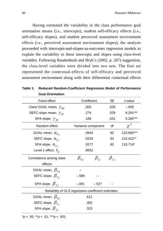
Table 1 presents results of this reduced random-coefficient regression model of performance goal orientation. As shown in Table 1,


on average, student self-efficacy was positively related to performance goal orientation within classrooms; 274.ˆ10 =γ , t(82) = 9.291, p < .001; suggesting that a one standard deviation increase in student self-efficacy was on average associated with a .274 standard deviation increase in performance goal orientation within classrooms. This relationship varied significantly across classrooms; 0229.1̂1 =τ , , p < .01. Also, on average, student perceived public assessment environment was positively related to performance goal orientation within classrooms;

412.124)82(2 =χ

166.ˆ20 =γ , t(82) = 5.284, p < .001; indicating that a one standard deviation increase in student perceived public assessment environment was on average associated with a .166 standard deviation increase in performance goal orientation within classrooms. This relationship varied significantly across classrooms; ,

, p < .05. 0277.ˆ22 =τ

714.110)82(2 =χAfter taking student self-efficacy and perceived public assessment

environment into account, the estimated within-class variance ( ) was reduced from .9436 in the random-effects ANOVA model to .8052. Hence, student self-efficacy and perceived public assessment environment accounted for about 15% of the within-class variance in performance goal orientation. As also shown in Table 1, the correlation between class mean performance goal orientation and self-efficacy slope ( = –.589) suggested that classes with high levels of performance goal orientation tended to be less differentiating with regard to student self-efficacy than were classes with low levels of performance goal orientation. The correlation between the random effects ( = –.527) suggested that there was sufficient independent variation to treat each of them as separate class effects. The estimates of the average class performance goal orientation as well as of the differentiating effects of self-efficacy and perceived public assessment environment were moderately reliable; = .611, .302, and .323 where q = 0, 1, and 2, respectively; suggesting sufficient observed variation to be explained in the intercepts ( ) and slopes ( where q = 1 and 2) using class characteristics.

2σ̂

01p̂

12p̂

)ˆ(ˆ qjβλ

j0β̂ qjβ̂


Having estimated the variability in the class performance goal orientation means (i.e., intercepts), student self-efficacy effects (i.e., self-efficacy slopes), and student perceived assessment environment effects (i.e., perceived assessment environment slopes), the analysis proceeded with intercepts-and-slopes-as-outcomes regression models to explain the variability in these intercepts and slopes using class-level variables. Following Raudenbush and Bryk’s (2002, p. 267) suggestion, the class-level variables were divided into two sets. The first set represented the contextual-effects of self-efficacy and perceived assessment environment along with their differential contextual effects

Table 1: Reduced Random-Coefficient Regression Model of Performance

Goal Orientation

Fixed effect Coefficient SE t-value

Class GOAL mean, 00γ .000 .035 –.005

SEFC slope mean, 10γ .274 .029 9.291***

SPA slope, 20γ .166 .031 5.284***

Random effect Variance component df 2χ

GOAL mean, ju0 .0644 82 210.665***

SEFC slope, ju1 .0229 82 124.412**

SPA slope, ju2 .0277 82 110.714*

Level-1 effect, ijr .8052

Correlations among class

effects j0β j1β j2β

GOAL mean, j0β –

SEFC slope, j1β –.589 –

SPA slope, j2β –.091 –.527 –

Reliability of OLS regression-coefficient estimates

GOAL mean, j0β .611

SEFC slope, j1β .302

SPA slope, j2β .323

*p < .05; **p < .01; ***p < .001


by class gender. The second set represented the joint effects of class gender, teacher’s teaching experience, and teacher’s assessment practices. Then, two submodels of the intercepts-and-slopes-as-outcomes regression model were fitted, one for each of the two sets of the class-level variables. For the sake of illustration, only the results pertaining to the first submodel are presented below.

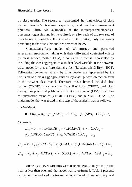
Contextual-effects model of self-efficacy and perceived assessment environment along with their differential contextual effects by class gender. Within HLM, a contextual effect is represented by including the class aggregate of a student-level variable in the between-class model for that differentiating effect (Raudenbush & Bryk, 2002). Differential contextual effects by class gender are represented by the inclusion of a class aggregate variable-by-class gender interaction term in the between-class model. Therefore, this submodel included class gender (GNDR), class average for self-efficacy (CEFC), and class average for perceived public assessment environment (CPA) as well as the interaction terms of (GNDR × CEFC) and (GNDR × CPA). The initial model that was tested in this step of the analysis was as follows.

Student-level:

ijjijjjijjjij rCPASPACEFCSEFCGOAL +−+−+= )()()( 210 βββ

Class-level:

jjj

jjjj

uCPAGNDRCEFCGNDR

CPACEFCGNDR

00504

030201000

)()(

)()()(

+×+×

++++=

γγ

γγγγβ

jjjj uCEFCGNDRCEFCGNDR 1131211101 )()()( +×+++= γγγγβ

jjjjj uCPAGNDRCPAGNDR 2232221202 )()()( +×+++= γγγγβ

Some class-level variables were deleted because they had t-ratios

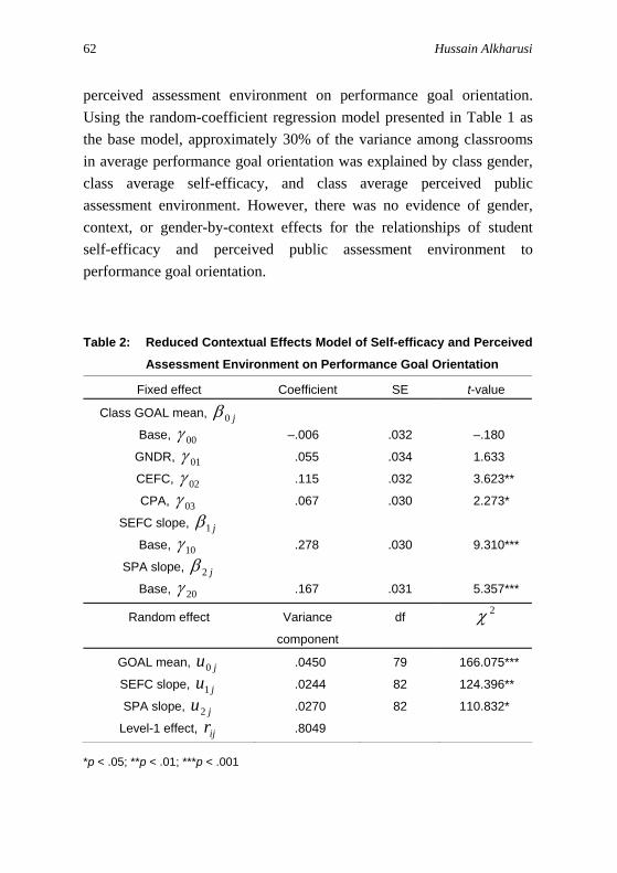
near or less than one, and the model was re-estimated. Table 2 presents results of the reduced contextual effects model of self-efficacy and


perceived assessment environment on performance goal orientation. Using the random-coefficient regression model presented in Table 1 as the base model, approximately 30% of the variance among classrooms in average performance goal orientation was explained by class gender, class average self-efficacy, and class average perceived public assessment environment. However, there was no evidence of gender, context, or gender-by-context effects for the relationships of student self-efficacy and perceived public assessment environment to performance goal orientation.

Table 2: Reduced Contextual Effects Model of Self-efficacy and Perceived

Assessment Environment on Performance Goal Orientation


Class GOAL mean, j0β

Base, 00γ –.006 .032 –.180

GNDR, 01γ .055 .034 1.633

CEFC, 02γ .115 .032 3.623**

CPA, 03γ .067 .030 2.273*

SEFC slope, j1β

Base, 10γ .278 .030 9.310***

SPA slope, j2β

Base, 20γ .167 .031 5.357***

Random effect Variance

component

df 2χ

GOAL mean, ju0 .0450 79 166.075***

SEFC slope, ju1 .0244 82 124.396**

SPA slope, ju2 .0270 82 110.832*

Level-1 effect, ijr .8049

*p < .05; **p < .01; ***p < .001


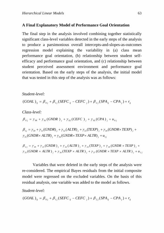
A Final Explanatory Model of Performance Goal Orientation

The final step in the analysis involved combining together statistically significant class-level variables detected in the early steps of the analysis to produce a parsimonious overall intercepts-and-slopes-as-outcomes regression model explaining the variability in (a) class mean performance goal orientation, (b) relationship between student self-efficacy and performance goal orientation, and (c) relationship between student perceived assessment environment and performance goal orientation. Based on the early steps of the analysis, the initial model that was tested in this step of the analysis was as follows:

Student-level:


Class-level:

jjjjj uCPACEFCGNDR 0030201000 )()()( ++++= γγγγβ

jjj

jjjjj

uALTRTEXPGNDRALTRGNDR

TEXPGNDRTEXPALTRGNDR

11615

14131211101

)()(

)()()()(

+××+×

+×++++=

γγ

γγγγγβ

jjjj

jjjjj

uALTRTEXPGNDRALTRTEXPALTRGNDR


2272625

24232221202

)()()(

)()()()(

+××+×+×

+×++++=

γγγ

γγγγγβ

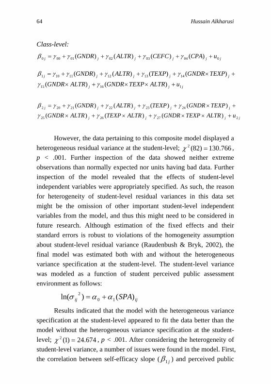
Variables that were deleted in the early steps of the analysis were re-considered. The empirical Bayes residuals from the initial composite model were regressed on the excluded variables. On the basis of this residual analysis, one variable was added to the model as follows.

Student-level:



Class-level:

jjjjjj uCPACEFCALTRGNDR 004030201000 )()()()( +++++= γγγγγβ

jjj

jjjjj

uALTRTEXPGNDRALTRGNDR


11615

14131211101

)()(

)()()()(

+××+×

+×++++=

γγ

γγγγγβ

jjjj

jjjjj

uALTRTEXPGNDRALTRTEXPALTRGNDR


2272625

24232221202

)()()(

)()()()(

+××+×+×

+×++++=

γγγ

γγγγγβ

However, the data pertaining to this composite model displayed a heterogeneous residual variance at the student-level; , p < .001. Further inspection of the data showed neither extreme observations than normally expected nor units having bad data. Further inspection of the model revealed that the effects of student-level independent variables were appropriately specified. As such, the reason for heterogeneity of student-level residual variances in this data set might be the omission of other important student-level independent variables from the model, and thus this might need to be considered in future research. Although estimation of the fixed effects and their standard errors is robust to violations of the homogeneity assumption about student-level residual variance (Raudenbush & Bryk, 2002), the final model was estimated both with and without the heterogeneous variance specification at the student-level. The student-level variance was modeled as a function of student perceived public assessment environment as follows:

766.130)82(2 =χ

ijij SPA)()ln( 102 αασ +=

Results indicated that the model with the heterogeneous variance specification at the student-level appeared to fit the data better than the model without the heterogeneous variance specification at the student-level; , p < .001. After considering the heterogeneity of student-level variance, a number of issues were found in the model. First, the correlation between self-efficacy slope (

674.24)1(2 =χ

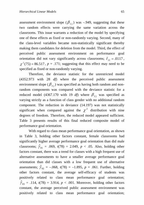
j1β ) and perceived public


assessment environment slope ( j2β ) was –.949, suggesting that these two random effects were carrying the same variation across the classrooms. This issue warrants a reduction of the model by specifying one of these effects as fixed or non-randomly varying. Second, many of the class-level variables became non-statistically significant thereby making them candidates for deletion from the model. Third, the effect of perceived public assessment environment on performance goal orientation did not vary significantly across classrooms; 0117.ˆ22 =τ ,

, p = .171; suggesting that this effect may need to be specified as fixed or non-randomly varying.

517.86)75(2 =χ

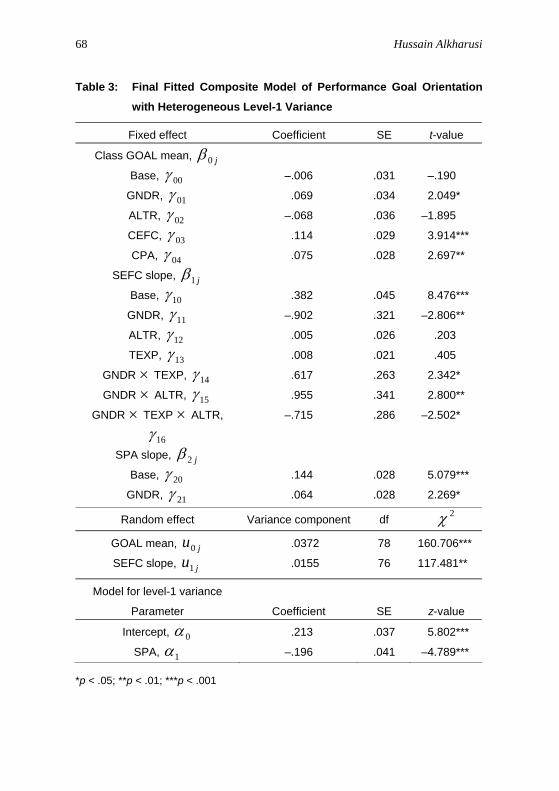
Therefore, the deviance statistic for the unrestricted model (4352.973 with 28 df) where the perceived public assessment environment slope ( j2β ) was specified as having both random and non-random components was compared with the deviance statistic for a reduced model (4367.170 with 19 df) where j2β was specified as varying strictly as a function of class gender with no additional random component. The reduction in deviance (14.197) was not statistically significant when compared against the distribution with nine degrees of freedom. Therefore, the reduced model appeared sufficient. Table 3 presents results of this final reduced composite model of performance goal orientation.

2χ

With regard to class mean performance goal orientation, as shown in Table 3, holding other factors constant, female classrooms had significantly higher average performance goal orientation than did male classrooms; 01γ̂ = .069, t(78) = 2.049, p < .05. Also, holding other factors constant, there was a trend for classes with a high frequent use of alternative assessments to have a smaller average performance goal orientation than did classes with a low frequent use of alternative assessments; 02γ̂ = –.068, t(78) = –1.895, p = .061. Further, holding other factors constant, the average self-efficacy of students was positively related to class mean performance goal orientation;

03γ̂ = .114, t(78) = 3.914, p < .001. Moreover, holding other factors constant, the average perceived public assessment environment was positively related to class mean performance goal orientation;


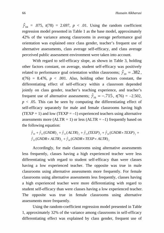
04γ̂ = .075, t(78) = 2.697, p < .01. Using the random coefficient regression model presented in Table 1 as the base model, approximately 42% of the variance among classrooms in average performance goal orientation was explained once class gender, teacher’s frequent use of alternative assessments, class average self-efficacy, and class average perceived public assessment environment were taken into account.

With regard to self-efficacy slope, as shown in Table 3, holding other factors constant, on average, student self-efficacy was positively related to performance goal orientation within classrooms; 382.ˆ10 =γ , t(76) = 8.476, p < .001. Also, holding other factors constant, the differentiating effect of self-efficacy within a classroom depended jointly on class gender, teacher’s teaching experience, and teacher’s frequent use of alternative assessments; 715.ˆ16 −=γ , t(76) = –2.502, p < .05. This can be seen by computing the differentiating effect of self-efficacy separately for male and female classrooms having high (TEXP = 1) and low (TEXP = –1) experienced teachers using alternative assessments more (ALTR = 1) or less (ALTR = –1) frequently based on the following equation:

jj

jjjj

ALTRTEXPGNDRALTRGNDR


)(ˆ)(ˆ)(ˆ)(ˆ)(ˆ)(ˆˆ

1615

1413121110

××+×

+×++++

γγ

γγγγγ

Accordingly, for male classrooms using alternative assessments less frequently, classes having a high experienced teacher were less differentiating with regard to student self-efficacy than were classes having a low experienced teacher. The opposite was true in male classrooms using alternative assessments more frequently. For female classrooms using alternative assessments less frequently, classes having a high experienced teacher were more differentiating with regard to student self-efficacy than were classes having a low experienced teacher. The opposite was true in female classrooms using alternative assessments more frequently.

Using the random-coefficient regression model presented in Table 1, approximately 32% of the variance among classrooms in self-efficacy differentiating effect was explained by class gender, frequent use of


alternative assessments, teaching experience, interaction of class gender-by-teaching experience, interaction of class gender-by-frequent use of alternative assessments, and interaction of class gender-by-teaching experience-by-frequent use of alternative assessments. As also shown in Table 3, performance goal orientation levels of students with a high perceived public assessment environment were higher; 144.ˆ20 =γ , t(1622) = 5.079, p < .001; and less variable; 196.ˆ1 −=α , z = –4.789, p < .001; than those for students with low levels of perceived public assessment environment. Also, the positive relationship between perceived public assessment environment and performance goal orientation tended to be stronger in female classrooms than in male classrooms; 064.ˆ21 =γ , t(1622) = 2.269, p < .05.

Conclusion

Given the research emphasis in the impact of educational assessment practices on student achievement-related outcomes, educational assessment researchers need to take advantage of the HLM as an appropriate analytic method for testing a variety of hypotheses about hierarchically structured data, as in the case of students nested within classrooms. Although the sample size requirements for HLM may not be feasible, it is nevertheless a versatile analytic approach to be utilized in educational assessment research to advance the research agenda in this area, in the sense that it does not only enable us to test hypotheses about effects occurring at each level of the hierarchy, but also estimates cross-level interaction effects that have received little empirical research attention.


Table 3: Final Fitted Composite Model of Performance Goal Orientation

with Heterogeneous Level-1 Variance


Class GOAL mean, j0β

Base, 00γ –.006 .031 –.190

GNDR, 01γ .069 .034 2.049*

ALTR, 02γ –.068 .036 –1.895

CEFC, 03γ .114 .029 3.914***

CPA, 04γ .075 .028 2.697**

SEFC slope, j1β

Base, 10γ .382 .045 8.476***

GNDR, 11γ –.902 .321 –2.806**

ALTR, 12γ .005 .026 .203

TEXP, 13γ .008 .021 .405

GNDR × TEXP, 14γ .617 .263 2.342*

GNDR × ALTR, 15γ .955 .341 2.800**

GNDR × TEXP × ALTR,

16γ

–.715 .286 –2.502*

SPA slope, j2β

Base, 20γ .144 .028 5.079***

GNDR, 21γ .064 .028 2.269*

Random effect Variance component df 2χ

GOAL mean, ju0 .0372 78 160.706***

SEFC slope, ju1 .0155 76 117.481**

Model for level-1 variance

Parameter Coefficient SE z-value

Intercept, 0α .213 .037 5.802***

SPA, 1α –.196 .041 –4.789***

*p < .05; **p < .01; ***p < .001


References

Alkharusi, H. (2008). Effects of classroom assessment practices on students’ achievement goals. Educational Assessment, 13(4), 243–266.

Bassiri, D. (1988). Large and small sample properties of maximum likelihood estimates for the hierarchical linear model (Unpublished doctoral dissertation). Michigan State University, East Lansing, MI, U.S.

Black, P., & Wiliam, D. (1998). Inside the black box: Raising standards through classroom assessment. Phi Delta Kappan, 80, 139–148.

Brookhart, S. M. (1994). Teachers’ grading: Practice and theory. Applied Measurement in Education, 7(4), 279–301.

Hox, J. (2002). Multilevel analysis: Techniques and applications. Mahwah, NJ: Lawrence Erlbaum.

Kreft, I., & Leeuw, J. D. (1998). Introducing multilevel modeling. London, England: Sage.

Mok, M. (1995). Sample size requirements for 2-level designs in educational research. Multilevel Modeling Newsletter, 7(2), 11–15.

Raudenbush, S. W. (1989). “Centering” predictors in multilevel analysis: Choices and consequences. Multilevel Modeling Newsletter, 1(2), 10–12.

Raudenbush, S. W., & Bryk, A. S. (2002). Hierarchical linear models: Applications and data analysis methods (2nd ed.). Thousand Oaks, CA: Sage.

Raudenbush, S. W., Bryk, A., Cheong, Y. F., & Congdon, R. (2004). HLM6: Hierarchical linear and nonlinear modeling. Lincolnwood, IL: Scientific Software International.

Raudenbush, S. W., & Liu, X. (2000). Statistical power and optimal design for multisite randomized trials. Psychological Methods, 5, 199–213.

Snijders, T. A. B., & Bosker, R. J. (1993). Standard errors and sample sizes for two-level research. Journal of Educational Statistics, 18, 237–259.

Snijders, T., & Bosker, R. (1999). Multilevel analysis: An introduction to basic and advanced multilevel modeling. London, England: Sage.

van der Leeden, R., & Busing, F. M. T. A. (1994). First iteration versus IGLS/RIGLS estimators in two-level models: A Monte Carlo study with ML3. Leiden Psychological Reports: Psychometrics and Research Methodology (pp. 1–21). Leiden, the Netherlands: Department of Psychology, University of Leiden.

Documents

Hierarchical Linear Models: Applications in Educational ...hkier.fed.cuhk.edu.hk/journal/wp-content/uploads/2011/10/erj_v26n1... · Hierarchical Linear Models 43 The Necessity for