Proving the Riemann Hypothesis Over the Zeros of the Zeta Function

Jesús Muñoz Vázquez@

Colegio de Postgraduados, Montecillo, México

Date: December 15, 2006

2000 Mathematics Subject Classification. Arithmetic.

Key words and phrases. Prime numbers , Riemann Hypothesis proved.

Dedication: to Chapingo

ABSTRACT. Abstract text...

Using functional calculus , an exact expression of the prime number function is obtained . With it , within a formula from Hilbert related to the Riemann Hypothesis , and also with the help of Mathematica 5.0 ; and his graphic capabilities , the eight problem of Hibert is solved

The graphics , let us to see clearly , the analytical results , of the different steps of the solution .

1. Section

Historical Background

The basic information we will utilize , can be found in several sources , the main ones are as follows : a poster named The Riemann Zeta Function with a draw of the zeta function on the “critical” line . In this display , we can find the concepts and equations relevant as antecedents to this paper .

The other main reference , is an article written by Enrico Bomberi about prime numbers in a scientific magazine . It describes what is known up to now , related to them , and includes a description of the intricacies of the prime number distribution . Also included is an anecdote , of how near Riemann was to find the exact distribution , illustrating its inspired try with a colored draw . What happens , to impede the solution , is that the function he found wriggles infinitely near integers , and consequently misses the exact prime number distribution function .

In Bomberi´s words : “in 1959 , the German mathematician Bernhard Riemann published his only paper in the theory of numbers , a truly astonishing tour de force on the distribution of primes .

“Rieman´s insight was that the frecuencies of the basic waveforms that approximate the psi function --an estimate or a manageable way of counting the number of primes less than , or equal to some number x-- are determined by the place where the zeta function is equal to zero . Thus one must solve the following equation for n :

1+1/ 2n+1/3n+1/4n…....= 0

To make it posible to find values of n , that will satisfy the equation , mathematicians apply certain tricks for handling infinite sums” . But the significant values for Riemann´s analysis are not just ordinary numbers ; rather they are complex numbers with two independents , values one real and one imaginary . The complex numbers that make the Riemann Zeta function equal to zero are the nontrivial zeros of the function . They occur in pairs , and there are infinitely many of them . Each one corresponds to an elementary wave form : the real part is the growth in its amplitude and the imaginary part is its frecuency (logarithmically plotted)”.

In Riemann´s analysis each complex number that acts as a zero function gives two kinds of information about the psi function. The real part controls, the large-scale behavior of the psi function --how quickly it ramps up . The imaginary part of each complex number, controls the smaller-scale , oscillatory effects . Thus, the values of the imaginary parts determine

precisely when Riemann´s elementary wave forms must be included in the “orchestra” to approximate the sharp steps taken by the psi function-- just as high-frecuency sine waves, made it, possible to approximate the sharp points of the sawtooth curve”.

“When the first 500 of Riemann´s elementary wave-forms are combined and the result is plotted, the curve first almost precisely the plot of psi (X) . The only deviation is overshooting at the corners in the curve-- the same effect one gets , by trying to add sine waves to approximate the sawtooth wave . You can see the overshooting if the lower-left corner of the graph is enlarged , as it is at left . To me , that the distribution of prime numbers , can be so accurately represented , in a hamonic analysis is absolutely amazing and incredibly beatiful . It tells of an arcane music and a secret harmony composed by the prime numbers. Did Riemann´s celebrated paper solve the main problem , explaning the regularities and irregularities in the distribution of the prime numbers? The aswer is no : mathematicians still want to understand the fine distribution of the primes . Riemann´s great accomplishment , was transfoming the problem of describing prime numbers , into the problem of describing the zeros of the Riemann zeta function-- which can be attacked directly” . “But it is by no means , trivial to solve . I am firmly convinced that the most important unsolved problems in mathematics today is the truth or falsity of a conjecture about the zeros of the zeta function , which was first made by Riemann himself . Suppose you plot the known zeros of the zeta fuction on a graph , the real part along the horizontal axis and the imaginary part along the vertical . In such a plot the complex zeros line up like soldiers along the vertical line that corresponds to the real value 1/2 , the so-called critical line . Riemann conjectured that the real part is always equal to 1/2 , for all the infinitely many zeros” .

Even a single exception , to Riemann´s conjeture would have enormously strange consecuences for the distribution of prime numbers . The primes appears to follow a kind of random distribution , and experiments with computers for large numbers of primes bear that out . If the Riemann Hypothesis , turns out to be false , there will be huge oscillations in the distribution of primes . In an orchestra , that would be like one loud instrument that drowns out the others-- an aesthetically distastefull situation” . “As a follower of William of Occam , said --"how elevate to a method the idea that when one must choose between two explanations , one should always choose the simpler” --I rejected that conclusion , and so I accept the truth of the Riemann hypothesis” . “As recently as two decades ago , virtually all mathematicians would have concurred with the common

perception about prime numbers : however worthy they may be of the most searching intellectual attention , they can have no utilily or application in the “real” world . How that has changed! Prime numbers and the methods of factoring large composites, are now at the heart of some of the most advanced methods of disguising data , to prevent unauthorized access. In this paper we try to solve , one important problem : the Hypothesis of Riemann . We are aware of the difficult task ; we know that some writers said “no layman understands it and no profesional can solve it” . But we are in the 21st century and we have some powerfull new weapons : functional calculus and its different versions , like Mikusinski operational calculus . In order to explain the inner aspects of the problem, we commend to read as soon as possible the book authored by Derbyshire ; just in case that the reader were no familiar with the theme . Besides , the book is free for the asking , specifically if you live in the underdeveloped world , as is my case.

OUTLINE

To solve the problem, we must finds first the prime number distribution formula, the one that give to us, the number of prime numbers up to any number N, This step is necessary, to deal with the formula of KOCH that defines the veracity of the Hypothesis of Riemann, in accord to the article of the Zeta function, published in the Mathematical Encyclopedia of Japan, and other articles, of similar nature.

HILBERT FORMULA

+ o ( In (n))as n infinity

� 2n dnInHnLﾏ!!!!nￛHnLﾙ

O is the big 0 of Landau (Helge Von Koch-1901) . Cited for Hilbert . We took from the book "Les nombres premieres" of Ellison and Mendes a transformation of the Koch formula , equivalent but simpler to work over it

.

Ellison Mendes Formula

The first term correspond to prime number distribution with the big O of Landau, and inside the parenthesis, the root of n (the variable) and the logarithm of the same variable, we are dealing with. What we need to do is to find the value of the expression when n tends to infinity. Our procedure will be, to transform the expression to operational calculus and find the value of the formula at the origin; this value, is well known is equal to the value at the limit, we are trying to find. We can consult the method used, as an example, in the book "Operational Calculus" by Van der Poll&Bremmer of Cambridge University Press-1964. In all the derivations of the procedure, we will use Mikusinskis Operational Calculus.

Related to the system used, we need to say that :

The operational Calculus was born, in the nineteen century, from Heaviside, that intituively derived useful methods to solve some differential equations. Latter, several mathematicians found similar results using the Laplacian Transform, and give to the calculus better basis. In the middle of the last century, Mikusinski, invent another version : he consider an abstract space of functions , with the common operations ; but instead of multiplication : convolution , and instead of division the inverse of convolution . If two functions, can not be divided , the result is an operator ; in the other case we have a realization . Inside the system we find an important operator (s) , the differential operator . So any function multiply for (s) gives, its differential, slighty different to the common definition . At the same time to divide by (s) is equivalent to integrate . In his book Mikusinski qualified his method , as better , comparing it , with the general concepts of the functional calculus , some authors sustain a similar concept ; besides we will go on precisely inside the operational concepts . To finish this comment ,we must say that, we are aware of some limitations of the method, but from my point of view,

ￛHnL- LiHnLﾏ!!!n log n

< Infinity

the are irrelevant to our discussion. In order to be as clear as posible, we will subdivide the work in different chapters, they are as follows.

1.-Finding the prime distribution formula .

a) Matrix of divisors .

b) Number of divisors of a number .

1) In algebra .

2) In Mathematica software .

3) In operational calculus .

c) Function with a number one (1) over every prime number , and with a number equal to the zero (0) over any other number .

1) In algebra .

2) In Mathematica software .

3) In operational calculus . d) Function that gives the number of prime numbers up to a number

N .

1) In algebra .

2) In Mathematica software .

3) In operational calculus .

In the literature , in past years , we was likely to find the idea , that the distribution of prime numbers , was devoid of regularity , and that , they obey only probabilistic laws .

What we will do is to presesnt a matrix that exhibits clearly its mathematical laws.

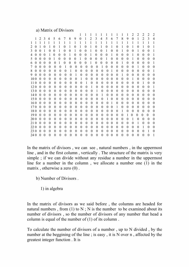
a) Matrix of Divisors

1 1 1 1 1 1 1 1 1 1 2 2 2 2 2 1 2 3 4 5 6 7 8 9 0 1 2 3 4 5 6 7 8 9 0 1 2 3 4 1 1 1 1 1 1 1 1 1 1 1 1 1 1 1 1 1 1 1 1 1 1 1 1 1 2 0 1 0 1 0 1 0 1 0 1 0 1 0 1 0 1 0 1 0 1 0 1 0 1 3 0 0 1 0 0 1 0 0 1 0 0 1 0 0 1 0 0 1 0 0 1 0 0 1 4 0 0 0 1 0 0 0 1 0 0 0 1 0 0 0 1 0 0 0 1 0 0 0 1 5 0 0 0 0 1 0 0 0 0 1 0 0 0 0 1 0 0 0 0 1 0 0 0 0 6 0 0 0 0 0 1 0 0 0 0 0 1 0 0 0 0 0 1 0 0 0 0 0 1 7 0 0 0 0 0 0 1 0 0 0 0 0 0 1 0 0 0 0 0 0 1 0 0 0 8 0 0 0 0 0 0 0 1 0 0 0 0 0 0 0 1 0 0 0 0 0 0 0 1 9 0 0 0 0 0 0 0 0 1 0 0 0 0 0 0 0 0 1 0 0 0 0 0 0 10 0 0 0 0 0 0 0 0 0 1 0 0 0 0 0 0 0 0 0 1 0 0 0 0 11 0 0 0 0 0 0 0 0 0 0 1 0 0 0 0 0 0 0 0 0 0 1 0 0 12 0 0 0 0 0 0 0 0 0 0 0 1 0 0 0 0 0 0 0 0 0 0 0 1 13 0 0 0 0 0 0 0 0 0 0 0 0 1 0 0 0 0 0 0 0 0 0 0 0 14 0 0 0 0 0 0 0 0 0 0 0 0 0 1 0 0 0 0 0 0 0 0 0 0 15 0 0 0 0 0 0 0 0 0 0 0 0 0 0 1 0 0 0 0 0 0 0 0 0 16 0 0 0 0 0 0 0 0 0 0 0 0 0 0 0 1 0 0 0 0 0 0 0 0 17 0 0 0 0 0 0 0 0 0 0 0 0 0 0 0 0 1 0 0 0 0 0 0 0 18 0 0 0 0 0 0 0 0 0 0 0 0 0 0 0 0 0 1 0 0 0 0 0 0 19 0 0 0 0 0 0 0 0 0 0 0 0 0 0 0 0 0 0 1 0 0 0 0 0 20 0 0 0 0 0 0 0 0 0 0 0 0 0 0 0 0 0 0 0 1 0 0 0 0 21 0 0 0 0 0 0 0 0 0 0 0 0 0 0 0 0 0 0 0 0 1 0 0 0 22 0 0 0 0 0 0 0 0 0 0 0 0 0 0 0 0 0 0 0 0 0 1 0 0 23 0 0 0 0 0 0 0 0 0 0 0 0 0 0 0 0 0 0 0 0 0 0 1 0 24 0 0 0 0 0 0 0 0 0 0 0 0 0 0 0 0 0 0 0 0 0 0 0 1

In the matrix of divisors , we can see , natural numbers , in the uppermost line , and in the first column , vertically . The structure of the matrix is very simple ; if we can divide without any residue a number in the uppermost line for a number in the column , we allocate a number one (1) in the matrix , otherwise a zero (0) .

b) Number of Divisors .

1) in algebra

In the matrix of divisors as we said before , the columns are headed for natural numbers , from (1) to N ; N is the number to be examined about its number of divisors , so the number of divisors of any number that head a column is equal of the number of (1) of its column .

To calculate the number of divisors of a number , up to N divided , by the number at the beggining of the line ; is easy , it is N over n , affected by the greatest integer function . It is

[ ] t ] he symbol [ ] means the greatest integer function .

The real problem is to calculate the number of (1) in any column , that is the number of divisors of a number N . That is what we try to do in the next paragraphs .

The variable is (n) , the lines of the matrix goes from 1 to N ; at the same time the columns goes from 1 to p , the extremun of the divisors we have under consideration . Later we will see as convenient to take squares of the matrix , that is to take n equal to p .

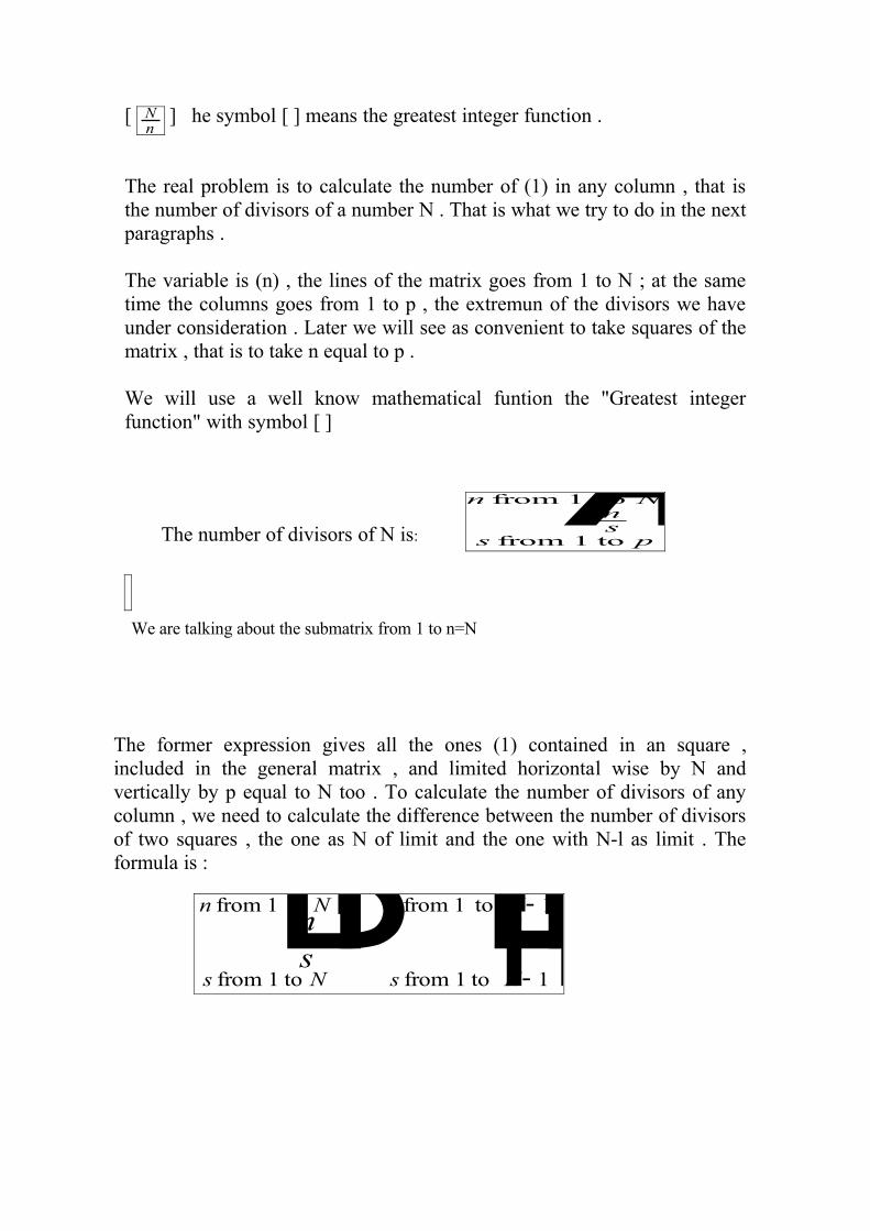
We will use a well know mathematical funtion the "Greatest integer function" with symbol [ ]

The number of divisors of N is:

We are talking about the submatrix from 1 to n=N

The former expression gives all the ones (1) contained in an square , included in the general matrix , and limited horizontal wise by N and vertically by p equal to N too . To calculate the number of divisors of any column , we need to calculate the difference between the number of divisors of two squares , the one as N of limit and the one with N-l as limit . The formula is :

Nn

ￚAnsEs from 1 to p

n from 1 to N

￢BnsFs from 1 to N

n from 1 to N

- ￢BnsFs from 1 toHN- 1Ln from 1 toHN- 1L

If the difference is a number two (2) we found a prime number .

2)Number of divisors, in mathematica software .

We are aware that there are several mathematical softwares that can be use to fullfil our purpose , any way we will employ Mathematica from Wolfram.

In Mathematica language :

P2[ n_] :=Sum[Floor[ n/i], {i, l,n}]P3 [n _]:=Sum[Floor[n-1/i], {i,l ,n}]P4[n_]:=P2[n]-P3[n]Plot[P4[n],{n,1,100}]

The last line let us to draw the divisors we are trying to find .

P2[n_] is a sub square of the general matrix and it give the number of divisors up to a number N . P3[n] is again a submatrix that give to us the number of divisors up to a number N-1 .

P4[n_] the difference of the sub matrices of the previous lines , gives to us the number of divisors of the number n . The last line of software , draw in the computer a graphic with the number of divisors of all the natural numbers between 1 and n , in this very case , 100 .

Graphic of the number of divisors from 1 to 100, giving the exact value for each number .

20 40 60 80 100

2

4

6

8

10

12

3) In operational calculus .

First we remember that in the divisors matrix , the function that gives the number of divisors of each natural number can be deducted , taking first the total number of (1) , that is of divisors in a sub matrix that finish with N , and substracting for that number the corresponding at the sub matrix N-l . In the functional calculus , we find an expression that represent in an exact way the distribution of ones (1) in a any line of the matrix ; in page 152 of Mikusinski Book , a formula (a) give to us , deltas of Dirac , with a space between them equal to λ , in the first line , deltas , one space apart , in the second two units apart , in the third , three units of separation ; and so on. The deltas of Dirac are well known ; have differential width and infinite altitud , they have an area of one unit ; with perfect resemblance to the lines of our matrix , The formulas are :

First Line 1111111111111111111111..........1/1-hSecond Line 0101010101010101010101...........1/1-h2 Third Line 0010010010010010010010............1/1-h3..........................................................................................n Line 1/1-hn

If we integrate any expression that represent any line ,we obtain , to any number n the sum of its divisors , and if we sum all the corresponding lines,we have now , the number of divisors of the submatrix , corres-ponding to that number .

As you saw , the operational formula , for each line is different of the Mikusinki book , and they are different because its representation are other of the lines of the matrix of divisors . In the matrix , every line beguins with zeroes , except the very first and the operational expressions from the book beguins with a one , that is delta of Dirac in the first place.Any way , we use now another formula from operational calculus , the one that let us move leftwise a function , the function is :

=

λ is the separation of the δ of Dirac in the functions described a few lines up,e is the basis of the Neperian logarithms , and λ is the most convenient symbol from n , the one that we use for the identification of the line or column of the matrix or both .

hl e- l s

To trascend the differences between the expressions in the Mikusinkis book an the divisors matrix , what we will do , is take the Mikusinskis expressions and translates them (n) places to the left , that is h places in order that the function beguins with zero as is in divisors matrix .

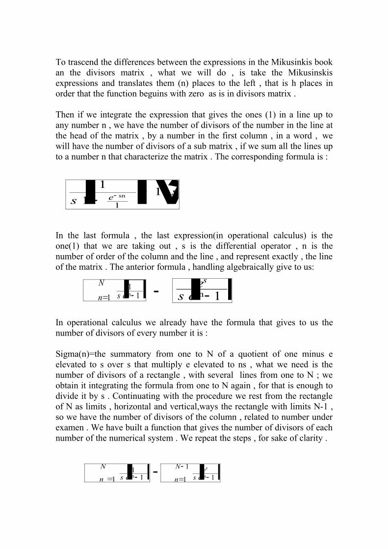
Then if we integrate the expression that gives the ones (1) in a line up to any number n , we have the number of divisors of the number in the line at the head of the matrix , by a number in the first column , in a word , we will have the number of divisors of a sub matrix , if we sum all the lines up to a number n that characterize the matrix . The corresponding formula is :

In the last formula , the last expression(in operational calculus) is the one(1) that we are taking out , s is the differential operator , n is the number of order of the column and the line , and represent exactly , the line of the matrix . The anterior formula , handling algebraically give to us:

-

In operational calculus we already have the formula that gives to us the number of divisors of every number it is :

Sigma(n)=the summatory from one to N of a quotient of one minus e elevated to s over s that multiply e elevated to ns , what we need is the number of divisors of a rectangle , with several lines from one to N ; we obtain it integrating the formula from one to N again , for that is enough to divide it by s . Continuating with the procedure we rest from the rectangle of N as limits , horizontal and vertical,ways the rectangle with limits N-1 , so we have the number of divisors of the column , related to number under examen . We have built a function that gives the number of divisors of each number of the numerical system . We repeat the steps , for sake of clarity .

- -

1

sI1 - e- sn

1M- 1ﾐs￢

n=1

N 1sHesn- 1L es

sHesn- 1L

￢n =1

N 1sHesn- 1L￢n=1

N- 1 es

sHesn- 1L

Note. If you want to check this formula, complicated, without doubt, you can draw a divisors matrix with the size you like; then draw the same matrix again, transport it to the left, you can see that the transported matrix, is exactly the matrix with limits N-1; that we are triying to find.

Function with a number (1) over a prime number and to the inverse of the number of its divisors over ony other number .

1) In algebra

Related to page 12 of this work we found a formula that give to us the number of divisors of any number it is :

the next step is to obtain a formula that give to us , 1 (one) over any prime number , otherwise a zero.

ikjjjjj￢JnsNs from 1, to N

n from 1, to N

-￢JnsNs from 1, to N- 1

n from 1, to N- 1y{zzzzzﾀﾂﾁﾁﾁﾁﾁﾁﾁﾁﾁﾁﾁﾁﾁﾁﾁﾁﾁ 2ￚInsM

s from 1, to N

n from 1, to N

- ￚInsMs from 1, to N- 1

n from 1, to N- 1

ﾃﾅﾄﾄﾄﾄﾄﾄﾄﾄﾄﾄﾄﾄﾄﾄﾄﾄﾄ@DIs the greatest integer symbol .

Formula with a number I over any prime number and over any other number a 0 (zero)

2) In Mathematica software

We remember , from the divisor matrix , that the function that gives the number of divisor of each number of the numerical system , can be deducted , taking first the number of divisors (that is ones (1) ) from a rectangle comprised from the origen to the number N , we are interested in .

Later we substract from the rectangle described in the previous , paragraphs , the ones (1) of a secund rectangle built from the origen to the number inmeadiately anterior , to which we are interest in , that is a number one less to N (that is N-l) .

P2[n_]:=Sum[Floor[n/i],{i,1,n}]P3[n_]:=Sum[Floor[(n/i)/i],{i,1,n}]P4 [n]:=P2[n]-P3[n]

P6 [n]:= Floor [2/P4[n] ]

After , we apply the greatest integer function , to one expression 2 over P6 . , what we have is a function with a number (1) one , over a prime number and a zero over any other number .

Plot [P6[n], {n, 1, 100} ]

20 40 60 80 100

0.5

1

1.5

2

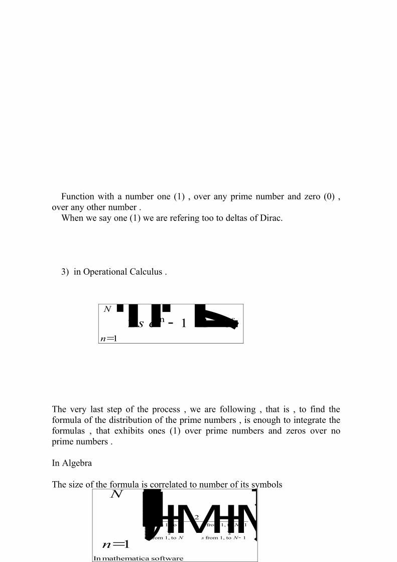
Function with a number one (1) , over any prime number and zero (0) , over any other number .

When we say one (1) we are refering too to deltas of Dirac.

3) in Operational Calculus .

The very last step of the process , we are following , that is , to find the formula of the distribution of the prime numbers , is enough to integrate the formulas , that exhibits ones (1) over prime numbers and zeros over no prime numbers .

In Algebra

The size of the formula is correlated to number of its symbols

￢n=1

NPP2 sHesn - 1Lﾐ1 - esT

n̄=1

N ﾀﾂﾁﾁﾁﾁﾁﾁﾁﾁﾁﾁﾁﾁﾁﾁﾁﾁﾁﾁﾁﾁﾁﾁﾁ 2ￚInsM

s from 1, to N

n from 1, to N

- ￚInsMs from 1, to N- 1

n from 1, to N- 1

ﾃﾅﾄﾄﾄﾄﾄﾄﾄﾄﾄﾄﾄﾄﾄﾄﾄﾄﾄﾄﾄ

Inmathematica software

p2[n_] : = Sum [ Floor [ n / 1 ], {i, 1, n} ]

p3 [n_] : = Sum [ Floor [ ( n - 1 ) / i ] , { i , 1 , n } ]

p4 [n_] : = p2 [ n ] - p3 [ n ]

p6 [n_] : = Floor [ 2 / p4 [ n ] ]

p7 [n_] : = Sum [ p6 [ j ] , { j , 1 , n } ]

Plot [ p7 [ n ] , { n , 1 , 10000 } ]

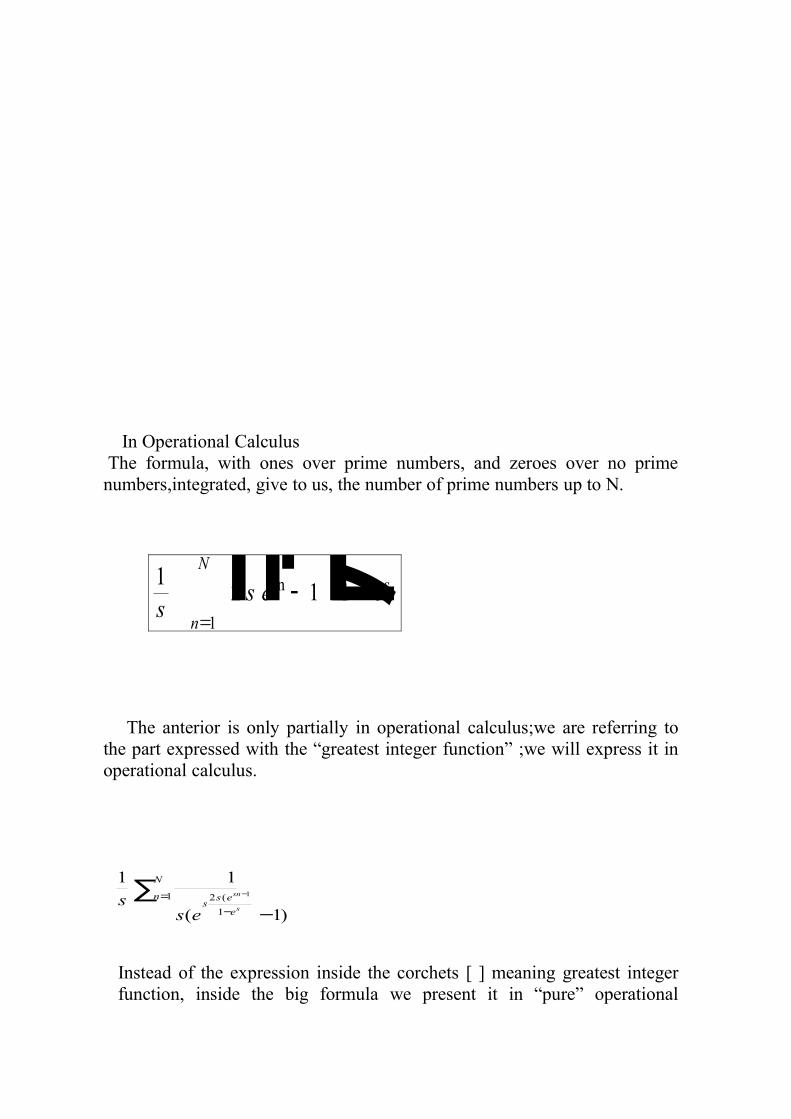
In Operational Calculus The formula, with ones over prime numbers, and zeroes over no prime numbers,integrated, give to us, the number of prime numbers up to N.

The anterior is only partially in operational calculus;we are referring to the part expressed with the “greatest integer function” ;we will express it in operational calculus.

∑=

− −−

N

n

e

ess

s

sn

ess 1

1

(2

)1(

111

Instead of the expression inside the corchets [ ] meaning greatest integer function, inside the big formula we present it in “pure” operational

1s￢n=1

NP2 sHesn - 1Lﾐ1 - esT

calculus. It come from a formula in Doestch book (page 252, formula 238).

The anterior formula is only partially in ooperational calculus, then we need to express too the “greatest integer function” in operational way.

[ ]=

We have now the prime number distribution formula in algebra, in Mathematica software and finally in operational calculus.

What follows is easy to enunciate and very difficult to comply ; the point is as follows: transform all the elements of the formula of Hilbert to operational language and with the use of a Tauberian formula calculate the limit.

We will begin repeating the Koch formula, cited for Hilbert in his famous intervention in the mathematical congress in Paris in 1901.

→ +o ( In (n) ) as n → infinity

Hilbert believed to prove it , as necessary for the prove of the Riemann Hypothesis.

ￛHnL� 1InHnL d nﾏ!!!n

ￛHnL- LiHnLﾏ!!!n log n< Infinity Again the equivalent EllisonMendez formula.

ta

____1____ s (esa – 1)

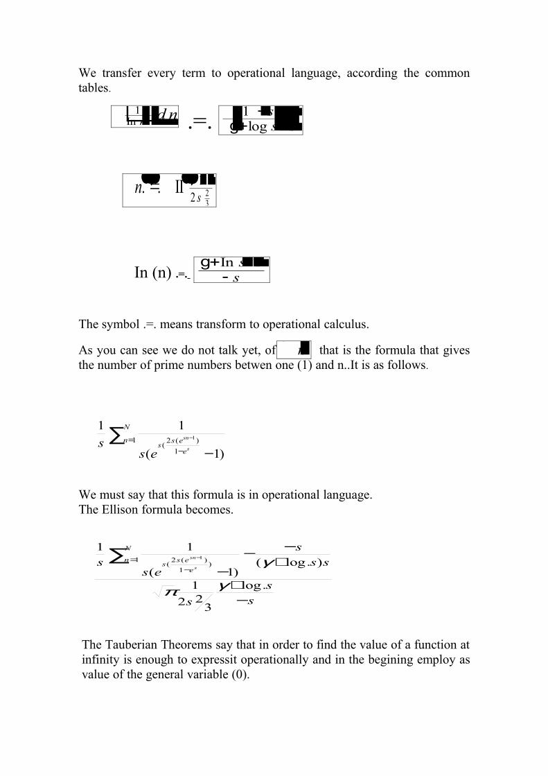
We transfer every term to operational language, according the common tables.

.=.

In (n) .=.

The symbol .=. means transform to operational calculus.

As you can see we do not talk yet, of that is the formula that gives the number of prime numbers betwen one (1) and n..It is as follows.

∑ =− −

−

N

n

e

ess

s

sn

ess 1

1

)(2(

)1(

111

We must say that this formula is in operational language.The Ellison formula becomes.

ss

s

sss

ess

N

n

e

ess

s

sn

−+

+−−

−∑=

−

−

.log

322

1

).log()1(

111

)1

)(2(

1

γπ

γ

The Tauberian Theorems say that in order to find the value of a function at infinity is enough to expressit operationally and in the begining employ as value of the general variable (0).

� 1InHnL d n 1 H- sLHg+logHsLL sﾏ!!!!n. =. ﾏ!!!!

II H1L2 s 2

3

ￛHnLg+InHsL 1

- s

In our case n=1 and s=0

As the value of the expression is 0 the Theorem of Riemann is proved.

The classic procedure is the substitution in the terms of the values of the variables by (0) zero.In the part of the formula that corresponds to prime number distribution n=1, the initial term.The value of the last formula in zero; then The Hilbert Hypotesis is proved.

REFERENCES

1. WOLFRAN RESEARCH INC. Software: Mathematica 5.0,

Champaign Illinois, 61820-7237, USA. 2. WOLFRAN RESEARCH INC. Poster: The Riemann Zeta Funetion,

Champaign Illinois, 61820-7237, USA. 3. HADAMARD, J Paper: Lectures on Cauchy's Problem in Linear

Partial Differential Equations, Dover Publieations, Ine, New York, (1952)

4. GELFAND, I.M and G.E. SHILOV. Book: Generalized Functions,Vols 1-3, Academic Press Ine., New York, (1964)

5. VAN DEL POL, B. and H. BREMMER. Book: Operational Calculus

on the Two-Sided Laplaee Transform, 2d ed., Cambridge University Press, (1955). "

6. DOESTCH, G. Book. A Guide to the Applieations of Laplace Transforms, D. Van Nostrand Company LTD, London, (1950), page 252, graph 238.

7. SCHWARTZ, L. Book: Théorie des distributions, Vols 1 and 11, Actualités Scientifiques et Industrielles, Hermann & Cie, Paris, France, (1957-1959).

8. MIKUSINSKI, J. Book: Operational Calculus, Pergamon Press, New York, (1959).

9. ERDÉRL Y, A. Book: Operational Calculus and Generalized Functions,Holt, Rinehart and Winston Ine., Athena Series, (1966), pages 80-125.

10. MATHEMATICAL SOCIETY OF JAPAN, Book: Encyclopedic

Dictionary, Article: Zeta Funtions, Second volume, (1980). 11. ROBINSON, A. Book: Non-Standard Analysis, Amsterdam, North

Holland, (1974). 12. ZEMANIAN A.H.Book: Operational Calculus and Distribution

Theory, Dover Publieations, Ine., New York, (1968). 13. JESUS MUÑOZ VAZQUEZ: Los Números Primos - 1960

14. Some notes related to Riemann hypothesis over the zeroes of the zeta function -1970 JESUS MUÑOZ VAZQUEZ.

ING. JESUS MUÑOZ VAZQUEZCamino a Santa Teresa No. 13, Edif. 5-1102Col. Héroes de PadiernaDeleg. Magdalena Contreras014400, México, D.F.Tel. Part. 28-76-80-67 (01-55)

Oficina: Municipio Libre No. 377,Col. Sta. Cruz Atoyac.C.P. 33669.Tel. 91-83-10-00 Ext. 33585j esusmunoz_20@yahoo.com.mx