Homework 3

Physics , Condensed MatterHomework

Due Tuesday, th October

Jacob Lewis Bourjaily

Problem 1: Electron in a Weak Sinusoidal Potential1

Consider an electron moving in a one-dimensional periodic potential U(r) = V cos (2πr/a). We are toobtain the eigenenergies ǫn(q) and corresponding wavefunctions ψn,q(r) of the lowest two bands, treatingthe potential perturbatively.

a) Away from the edge of the Brillouin zone, there are no degeneracies in the lowest energy band.Using this fact, we are to compute ǫ1(q) to order V 2 and the corresponding wavefunctions to order V .

We begin by doing what amounts to Fourier transforming ψ(r) into momentum space,making use of Bloch’s theorem to write

ψq(r) =∑

G

cq−Gei(q−G)r, (1.a.1)

where G represents the reciprocal lattice, which is in this one-dimensional problemgenerated simply by b ≡ 2π

a . Following Ashcroft and Mermin, we will study theSchrodinger equation in momentum space:

[

~2

2m(q −G) − ǫ

]

cq−G +∑

G′

UG′−Gcq−G = 0, (1.a.2)

where Uk are Fourier modes of the potential. In our case, this is extremely easyto extract: every kindergartener should be able to take the Fourier transform of acosine; we find:

U+1 = U−1 =V

2and Ui6=±1 = 0. (1.a.3)

We are going to be interested in a wave function concentrated well within the firstBrillouin zone, in the limit where there are no nearly degenerate bands. Writing

ǫ0q = ~2

2mq2 and inserting our potential Uk into the Schrodinger equation, we see

(

ǫ− ǫ0q)

cq =V

2(cq+b + cq−b) =⇒ cq =

V

2(ǫ− ǫ0q)(cq+b + cq−b) . (1.a.4)

This expression does not reflect our interest in the first Brillouin zone: it is validfor all q. Indeed, we see that we can iteratively unfold the equation to obtain anexpansion in terms of V

2(ǫ−ǫ0q′

):

cq =V

2(ǫ− ǫ0q)(cq+b + cq−b) , (1.a.5)

=V

2(ǫ− ǫ0q)

{

V

2(ǫ− ǫ0q+b)(cq + cq+2b) +

V

2(ǫ− ǫ0q−b)(cq + cq−2b)

}

, (1.a.6)

=V 2cq

4(ǫ− ǫ0q)

{

1

(ǫ− ǫ0q+b)+

1

(ǫ− ǫ0q−b)

}

+

[

V 3

8(ǫ− ǫ0q)(ǫ− ǫ0q+b)(ǫ− ǫ0q+2b)(cq+b + cq+3b) + (b↔ −b)

]

;

(1.a.7)

&tc. Now, because we are expanding in V2(ǫ−ǫ0q) , we may safely drop the O(V 3)

terms. Also, notice that in the curly brackets that we have the expressions ǫ− ǫ0q±b.Now, because the bands are non-degenerate and we know the band energies are onlyaffected by terms leading in V 2, we can are allowed to take (ǫ− ǫ0q±b) 7→ (ǫ0q − ǫ0q±b)to this order of approximation. With that in mind, we may divide both sides of theexpression above by cq/(ǫ− ǫ0q) obtaining

(ǫ− ǫ0q) =V 2

4

{

1

(ǫ0q − ǫ0q+b)+

1

(ǫ0q − ǫ0q−b)

}

+ O(V 3). (1.a.8)

1Note added in revision: the solution presented follows Ashcroft and Mermin—which is absolutely horrendous. Theentire first problem can be done in a couple of lines if you read the first few pages of Griffith’s Quantum Mechanics chapteron (time independent) perturbation theory first! Honestly, believe me; learn non-degenerate perturbation theory first (andsee how to apply it in the degenerate case) and the problem will be MUCH easier.

1

2 JACOB LEWIS BOURJAILY

It is not altogether delightful, but this expression can of course be quite dramaticallysimplified.

ǫ = ǫ0q +V 22m

4~2b

{

2q + b− 2q + b

(4q2 − b2)

}

+ O(V 3),

= ǫ0q +V 2m

~2

{

1

(4q2 − 4π2

a2 )

}

+ O(V 3),

∴ ǫ =~

2

2mq2 +

V 2m

4~2(

q2 − π2

a2

) + O(V 3). (1.a.9)

‘oπǫρ ’ǫδǫι πoι�ησαι

Now we are asked to determine the corrected wave function to leading order in V . Todo this, we start by combining the right hand sides of equations (1.a.5) and (1.a.7):

V

2(ǫ− ǫ0q)(cq+b + cq−b) =

V 2cq4(ǫ− ǫ0q)

{

1

(ǫ0q − ǫ0q+b)+

1

(ǫ0q − ǫ0q−b)

}

+ O(V 3),

=⇒ (cq+b + cq−b) = cqV

2

{

1

(ǫ0q − ǫ0q+b)+

1

(ǫ0q − ǫ0q−b)

}

+ O(V 2),

= cqV m

2~2(

q2 − π2

a2

) + O(V 2). (1.a.10)

Now, remember that equation (1.a.4) allows to write cq−b in terms of cq and cq−2b, forexample. Using this to rearrange equation (1.a.10), we see

cq+b = −cq−b + cqV m

2~2(

q2 − π2

a2

) + O(V 2),

= − V

2(ǫ0q − ǫ0q−b)(cq + cq−2b) + cq

V m

2~2(

q2 − π2

a2

) + O(V 2),

= cq

{

V m

2~2(

q2 − π2

a2

) − V

2(ǫ0q − ǫ0q−b)

}

+ O(V 2),

= cqV m

2~2(

q2 − π2

a2

)

{

1 − 1

2π(aq + π)

}

+ O(V 2);

∴ cq+b = cqVm

4~2(

q2 − π2

a2

)

(

1 − aq

π

)

+ O(V 2). (1.a.11)

We don’t need to reproduce the above steps for cq−b: it comes for free once we havecq+b:

cq−b = −cq+b + cqV m

2~2(

q2 − π2

a2

) + O(V 2),

= cqV m

2~2(

q2 − π2

a2

)

(

1 − 1

2

(

1 − qa

π

)

)

+ O(V 2);

∴ cq−b = cqV m

4~2(

q2 − π2

a2

)

(

1 +qa

π

)

+ O(V 2). (1.a.12)

Inserting this in the expansion for ψq(r), we find directly,

ψq(r) = cqeiqr + cq+be

iqreibr + cq−beiqre−ibr + O(V 2),

= cqeiqr

{

1 +V m

4~2(

q2 − π2

a2

)

[(

1 − aq

π

)

eirb +(

1 +qa

π

)

e−irb]

}

+ O(V 2);

∴ ψq(r) = cqeiqr

{

1 +V m

2~2(

q2 − π2

a2

)

(

cos

(

2πr

a

)

− iqa

πsin

(

2πr

a

)

)

}

. (1.a.13)


PHYSICS : CONDENSED MATTER HOMEWORK 3

b) At the edge of the Brillouin zone there are degeneracies for small V . We are to work pertur-batively near the zone edge to diagonalize the single electron Hamiltonian within the two-state Hilbertspace of the two nearly-degenerate lowest-energy free-electron momentum eigenstates of the same crystalmomentum. Then, we are to add the effects of the higher bands perturbatively. We are to obtain theeigenenergies of the lowest two energy bands to order V 2 and the wave functions to order V as before.We are to verify that for small V these results match our work for part (a) when one moves far enoughaway from the edge of the Brillouin zone. We are to sketch the dispersions ǫn(q) and determine howsmall V must be for this perturbation analysis to be reliable.

We are going to proceed along lines similar to those encountered in part (a). Specifically,let us start by again by equating the right hand sides of equations (1.a.5) and (1.a.7)—only this time, we will not use the assumption that all the eigenenergies are non-degenerate.

(ǫ− ǫ0q) =V 2

4

{

1

(ǫ− ǫ0q+b)+

1

(ǫ− ǫ0q−b)

}

+ O(V 3). (1.b.14)

Now, we are going to consider perturbing the system near the Bragg plane at q = πa ;

this will mean that we can consider the term ǫ− ǫ0q+b ≡ ζ where 1/ζ is at most linearin V—we will justify this and give an explicit expression for ζ later.

Manipulating equation (1.b.14), we see that

(

ǫ− ǫ0q)

(ǫ− ǫq−b) =V 2

4

(

1 +ǫ− ǫ0q−b

ζ

)

+ O(V 3),

=⇒ ǫ2 − ǫ

(

ǫ0q + ǫ0q−b +V 2

4ζ

)

+ ǫ0qǫ0q−b −

V 2

4

(

1 −ǫ0q−b

ζ

)

= 0.

This quadratic is easily solved by calling upon kindergarten identities:

ǫ =1

2

(

ǫ0q + ǫ0q−b +V 2

4ζ

)

± 1

2

{

(

ǫ0q + ǫ0q−b +V 2

4ζ

)2

− 4ǫ0qǫ0q−b + V 2

(

1 −ǫ0q−b

ζ

)}1/2

;

∴ ǫ =1

2

(

ǫ0q + ǫ0q−b +V 2

4ζ

)

± 1

2

{

(

ǫ0q − ǫ0q−b +V 2

4ζ

)2

+ V 2

}1/2

. (1.b.15)


To evaluate the expression, one can simply insert the equation itself iteratively intoζ = ǫ − ǫ0q+b—and observe that that it always gives a well-defined expression up to

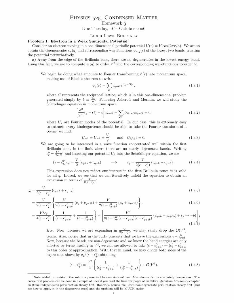
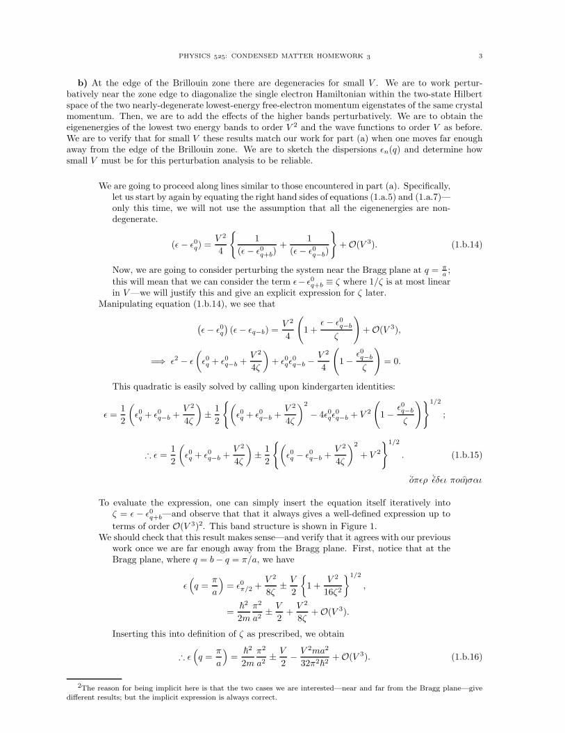
terms of order O(V 3)2. This band structure is shown in Figure 1.We should check that this result makes sense—and verify that it agrees with our previous

work once we are far enough away from the Bragg plane. First, notice that at theBragg plane, where q = b− q = π/a, we have

ǫ(

q =π

a

)

= ǫ0π/2 +V 2

8ζ± V

2

{

1 +V 2

16ζ2

}1/2

,

=~

2

2m

π2

a2± V

2+V 2

8ζ+ O(V 3).

Inserting this into definition of ζ as prescribed, we obtain

∴ ǫ(

q =π

a

)

=~

2

2m

π2

a2± V

2− V 2ma2

32π2~2+ O(V 3). (1.b.16)

2The reason for being implicit here is that the two cases we are interested—near and far from the Bragg plane—givedifferent results; but the implicit expression is always correct.


0 0.5 1 1.5 2 2.5 3

Momentum q

0

10

20

30

40

ygre

nE

eula

vne

giE

Figure 1. The second-order band structure for a one-dimensional system in a weaksinusoidal potential.

Similarly, we can check that equation (1.b.15) gives the right answer when we are farenough away from the Bragg plane. When we are far from the Bragg plane, thenǫ0q − ǫ0q−b ≫ V 2 so that we may expand

ǫ =1

2

(

ǫ0q + ǫ0q−b +V 2

4ζ

)

± 1

2

{

(

ǫ0q − ǫ0q−b +V 2

4ζ

)2

+ V 2

}1/2

,

=1

2

ǫ0q + ǫ0q−b +V 2

4ζ±(

ǫ0q − ǫ0q−b

)

V 2

(

ǫ0q − ǫ0q−b

)2 +

1 +V 2

4ζ(

ǫ0q − ǫ0q−b

)

2

1/2

,

=1

2

ǫ0q + ǫ0q−b +V 2

4ζ±(

ǫ0q − ǫ0q−b

)

1 +V 2

(

ǫ0q − ǫ0q−b

)2 +V 2

2ζ(

ǫ0q − ǫ0q−b

) + O(V 4)

1/2

,

=1

2

ǫ0q + ǫ0q−b +V 2

4ζ±

(

ǫ0q − ǫ0q−b

)

+V 2

2(

ǫ0q − ǫ0q−b

) +V 2

4ζ+ O(V 4)

.

Taking the solution corresponding to the lower band3,

ǫ1(q) = ǫ0q +V 2

4

{

1

2ζ+

1

ǫ0q − ǫ0q−b

+1

2ζ

}

+ O(V 3),

= ǫ0q +V 2

4

{

1

ǫ0q − ǫ0q+b

+1

ǫ0q − ǫ0q−b

}

+ O(V 3),

and this we recognize as equation (1.a.8), which implies that this formula (1.b.15)does indeed agree with our results from part (a).


Our last task is to determine the wave function for electrons at the Bragg plane to firstorder in V . We will follow similar lines of thought to those travelled in part (a). Usingthe same logic as there—only this time being careful not to ignore degeneracies—wecan begin our work with the equations

cq+b + cq−b = cqV

2

{

1

(ǫ− ǫ0q+b)+

1

(ǫ− ǫ0q−b)

}

+ O(V 2) and cq =V

2(ǫ− ǫ0q)(cq+b + cq−b) . (1.b.17)

3The solutions corresponding to the respective ‘±’ sign the equation (1.b.15) have now switched—this is simply because

when we extracted�ǫ0q − ǫ0

q−b

�from the square root, the signs one again become arbitrarily assigned.


This system yields exactly our result in part (a) for the case of cq+b:

cq+b = cqV

2

{

1

(ǫ− ǫ0q+b)+

1

(ǫ− ǫ0q−b)

}

− cb−q + O(V 2),

cq+b = cqV

2

{

1

(ǫ− ǫ0q+b)+

1

(ǫ− ǫ0q−b)− 1

(ǫ− ǫ0q−b)

}

+ O(V 2),

cq+b = cqV

2(ǫ− ǫ0q+b)+ O(V 2),

cq+b = cqV

2(ǫ0q − ǫ0q+b)+ O(V 2),

= −cqV 2ma

4π~2(q + πa )

+ O(V 2);

∴ cq+b = cqV 2

4~2(

q2 − π2

a2

)

(

1 − qa

π

)

+ O(V 2). (1.b.18)

The story changes, however, for cq−b. It is not hard to jump a bit in the calculation andsee

cq−b = cqV

2(ǫ− ǫ0q−b)+ O(V 2). (1.b.19)

Now, from our calculation of the eigenenergies at the Bragg plane we know that

ǫπ/a − ǫ0π/a−b = ±V2− V 2ma

16π~2(

q + πa

) + O(V 3), (1.b.20)

so we see

cq−b = cqV

2

(

±V2 − V 2ma

16π~2(q+ πa )

) + O(V 2),

= cq1

±(

1 ∓ V 2ma

8π~2(q+ πa )

) + O(V 2),

∴ cq−b = ±cq(

1 +V m

8~2(

q2 − π2

a2

)

(qa

π− 1)

)

+ O(V 2). (1.b.21)

Putting all this together, we see

ψ±q= π

a(r) = cqe

iqr

{

1 ± e−ibr +V m

4~2(

q2 − π2

a2

)

(

1 − aq

π

)

(

eibr ∓ e−ibr

2

)

}

,

so that

ψ+(r) ∝ cqeiqr

{

2e−i br2 cos

(πr

a

)

+ iV m

2~2(

q2 − π2

a2

)

(

1 − aq

π

)

[

sin

(

2πr

a

)

− ie−ibr

4

]

}

; (1.b.22)

and

ψ−(r) ∝ cqeiqr

{

2ie−i br2 sin

(πr

a

)

+V m

2~2(

q2 − π2

a2

)

(

1 − aq

π

)

[

cos

(

2πr

a

)

− e−ibr

4

]

}

. (1.b.23)



-0.4

-0.2

0

0.2

0.4

-0.4

-0.2

0

0.2

0.4

-2

-1

0

1

2

-0.4

-0.2

0

0.2

0 4

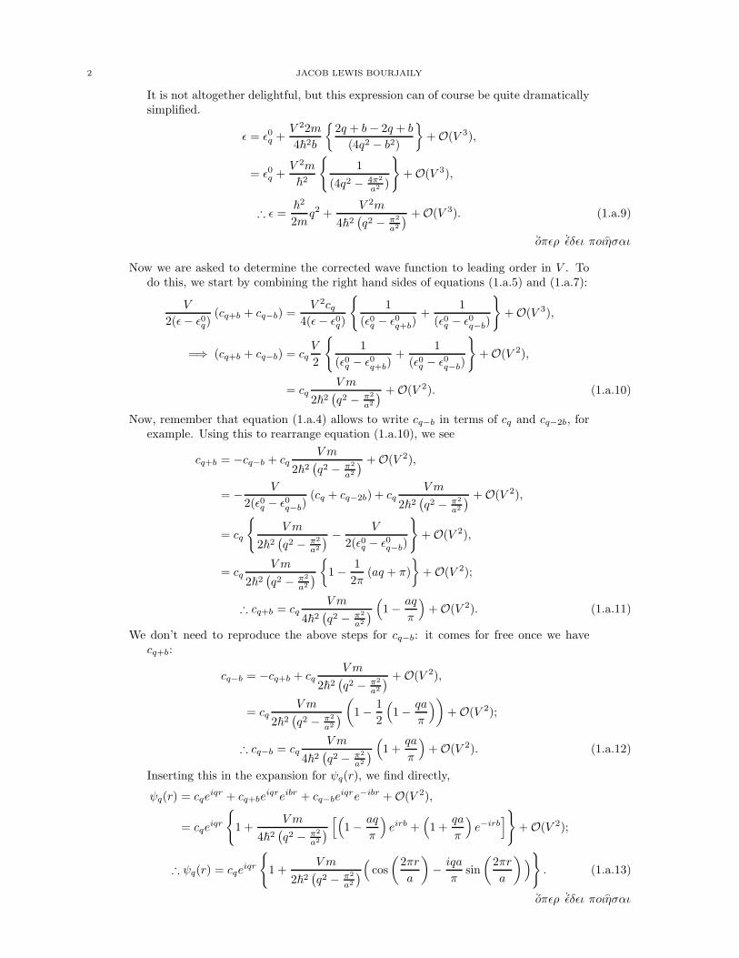
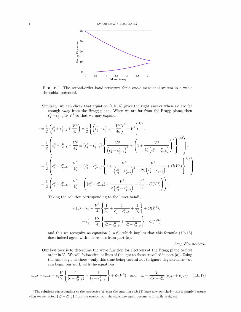
Figure 2. The first Brillouin zone dispersion for a tight-binding model on a two-dimensional square lattice.

Problem 2: Tight-Binding Model on a Square LatticeConsider a tight-binding model on a square, two-dimensional square lattice (lattice spacing a) with

on-site energy ǫ0 and nearest-neighbour hopping matrix element t:

H =∑

r

{

ǫ0|r〉〈r| + t[

|r〉〈r + ax| + |r〉〈r − ax| + |r〉〈r + ay| + |r〉〈r − ay|]}

.

a) We are to obtain the dispersion relation for this model.

Just for the sake of clearing up notation, our Bravais lattice here will be generated by~a1 = a(1, 0) and ~a2 = a(0, 1) which has the associated reciprocal lattice generated by~b1 = 2π

a (1, 0) and ~b2 = 2πa (0, 1). We will write all momenta in terms of the reciprocal

lattice, so ~q = q1~b1 + q2~b2. Using Bloch’s theorem it is quite easy to see that theHamiltonian of this system is given by

Hψ ={

ǫ0 + t(

ei~q·~a1 + e−i~q·~a1 + ei~q·~a2 + e−i~q·~a2

)}

ψ, (2.a.1)

={

ǫ0 + t(

ei2πq1 + e−i2πq1 + ei2πq2 + e−i2πq2

)}

ψ, (2.a.2)

={

ǫ0 + 2t (cos (2πq1) + cos (2πq2))}

ψ; (2.a.3)

∴ ǫ(~q) = ǫ0 + 2t {cos(2πq1) + cos(2πq2)} . (2.a.4)

This dispersion relation is shown in the first Brillouin zone in Figure 2.

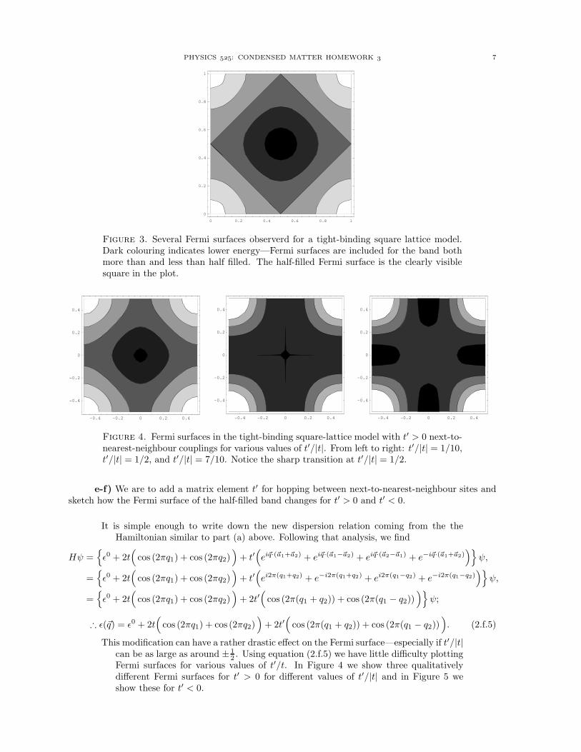
b-d) Let us sketch the Fermi surface in the first Brillouin zone when the band is less than and morethan half-full, assuming a particle-like band (t < 0). And we are to make an accurate drawing of theFermi surface for the case of a precisely half-filled band.

When the Fermi surface is very near the bottom of the band energy, then it is ap-proximately a circle: for qi ≪ 1, we can expand the cos(2πqi)’s to see that ǫ(q) ∼ǫ0 + 2t− 2πt~q 2 + O(~q 3), the solution to which is precisely a circle.

As the energy increases, the Fermi surface flattens out along the diagonal directions,becoming a square when the band is half-filled. When the band is more than half-filled, the square breaks into four disjoint components which encircle the corners ofthe Brillouin zone. Expanding cos (2πqi) about qi ∼ 1

2 shows that when the band isnearly filled, the Fermi surface components do in fact become circles.

These are shown in detail in Figure 3.


0 0.2 0.4 0.6 0.8 1

0

0.2

0.4

0.6

0.8

1

Figure 3. Several Fermi surfaces observerd for a tight-binding square lattice model.Dark colouring indicates lower energy—Fermi surfaces are included for the band bothmore than and less than half filled. The half-filled Fermi surface is the clearly visiblesquare in the plot.

-0.4 -0.2 0 0.2 0.4

-0.4

-0.2

0

0.2

0.4

-0.4 -0.2 0 0.2 0.4

-0.4

-0.2

0

0.2

0.4

-0.4 -0.2 0 0.2 0.4

-0.4

-0.2

0

0.2

0.4

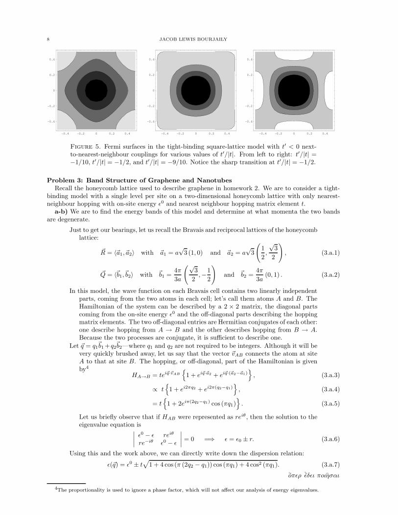
Figure 4. Fermi surfaces in the tight-binding square-lattice model with t′ > 0 next-to-nearest-neighbour couplings for various values of t′/|t|. From left to right: t′/|t| = 1/10,t′/|t| = 1/2, and t′/|t| = 7/10. Notice the sharp transition at t′/|t| = 1/2.

e-f) We are to add a matrix element t′ for hopping between next-to-nearest-neighbour sites andsketch how the Fermi surface of the half-filled band changes for t′ > 0 and t′ < 0.

It is simple enough to write down the new dispersion relation coming from the theHamiltonian similar to part (a) above. Following that analysis, we find

Hψ ={

ǫ0 + 2t(

cos (2πq1) + cos (2πq2))

+ t′(

ei~q·(~a1+~a2) + ei~q·(~a1−~a2) + ei~q·(~a2−~a1) + e−i~q·(~a1+~a2))}

ψ,

={

ǫ0 + 2t(


+ t′(

ei2π(q1+q2) + e−i2π(q1+q2) + ei2π(q1−q2) + e−i2π(q1−q2))}

ψ,

={

ǫ0 + 2t(


+ 2t′(

cos (2π(q1 + q2)) + cos (2π(q1 − q2)))}

ψ;

∴ ǫ(~q) = ǫ0 + 2t(


+ 2t′(

cos (2π(q1 + q2)) + cos (2π(q1 − q2)))

. (2.f.5)

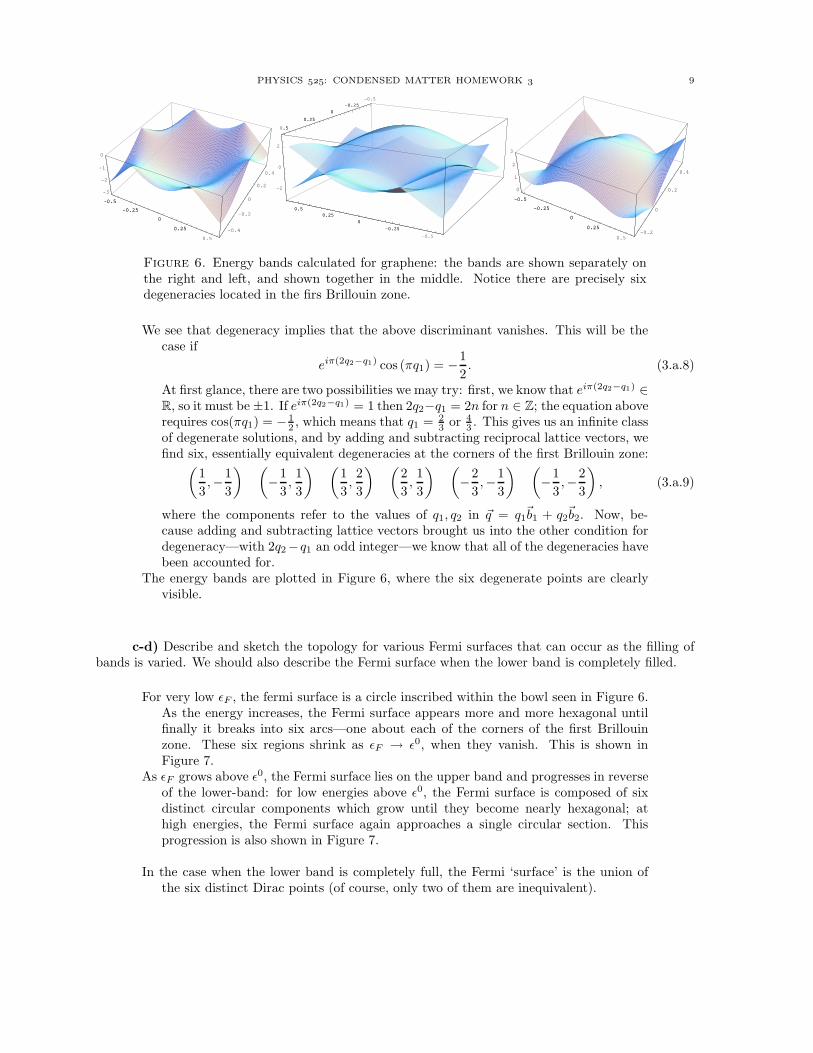
This modification can have a rather drastic effect on the Fermi surface—especially if t′/|t|can be as large as around ± 1

2 . Using equation (2.f.5) we have little difficulty plottingFermi surfaces for various values of t′/t. In Figure 4 we show three qualitativelydifferent Fermi surfaces for t′ > 0 for different values of t′/|t| and in Figure 5 weshow these for t′ < 0.


-0.4 -0.2 0 0.2 0.4

-0.4

-0.2

0

0.2

0.4

-0.4 -0.2 0 0.2 0.4

-0.4

-0.2

0

0.2

0.4

-0.4 -0.2 0 0.2 0.4

-0.4

-0.2

0

0.2

0.4

Figure 5. Fermi surfaces in the tight-binding square-lattice model with t′ < 0 next-to-nearest-neighbour couplings for various values of t′/|t|. From left to right: t′/|t| =−1/10, t′/|t| = −1/2, and t′/|t| = −9/10. Notice the sharp transition at t′/|t| = −1/2.

Problem 3: Band Structure of Graphene and NanotubesRecall the honeycomb lattice used to describe graphene in homework 2. We are to consider a tight-

binding model with a single level per site on a two-dimensional honeycomb lattice with only nearest-neighbour hopping with on-site energy ǫ0 and nearest neighbour hopping matrix element t.

a-b) We are to find the energy bands of this model and determine at what momenta the two bandsare degenerate.

Just to get our bearings, let us recall the Bravais and reciprocal lattices of the honeycomblattice:

~R = 〈~a1,~a2〉 with ~a1 = a√

3 (1, 0) and ~a2 = a√

3

(

1

2,

√3

2

)

, (3.a.1)

~Q = 〈~b1,~b2〉 with ~b1 =4π

3a

(√3

2,−1

2

)

and ~b2 =4π

3a(0, 1) . (3.a.2)

In this model, the wave function on each Bravais cell contains two linearly independentparts, coming from the two atoms in each cell; let’s call them atoms A and B. TheHamiltonian of the system can be described by a 2 × 2 matrix, the diagonal partscoming from the on-site energy ǫ0 and the off-diagonal parts describing the hoppingmatrix elements. The two off-diagonal entries are Hermitian conjugates of each other:one describe hopping from A → B and the other describes hopping from B → A.Because the two processes are conjugate, it is sufficient to describe one.

Let ~q = q1~b1 +q2~b2—where q1 and q2 are not required to be integers. Although it will bevery quickly brushed away, let us say that the vector ~vAB connects the atom at siteA to that at site B. The hopping, or off-diagonal, part of the Hamiltonian is givenby4

HA→B = tei~q·~vAB

{

1 + ei~q·~a2 + ei~q·(~a2−~a1)}

, (3.a.3)

∝ t{

1 + ei2πq2 + ei2π(q2−q1)}

, (3.a.4)

= t{

1 + 2eiπ(2q2−q1) cos (πq1)}

. (3.a.5)

Let us briefly observe that if HAB were represented as reiθ , then the solution to theeigenvalue equation is

∣

∣

∣

∣

ǫ0 − ǫ reiθ

re−iθ ǫ0 − ǫ

∣

∣

∣

∣

= 0 =⇒ ǫ = ǫ0 ± r. (3.a.6)

Using this and the work above, we can directly write down the dispersion relation:

ǫ(~q) = ǫ0 ± t√

1 + 4 cos (π (2q2 − q1)) cos (πq1) + 4 cos2 (πq1). (3.a.7)


4The proportionality is used to ignore a phase factor, which will not affect our analysis of energy eigenvalues.


-0.5

-0.25

0

0.25

0.5

-0.4

-0.2

0

0.2

0.4

-3

-2

-1

0

-0.5

-0.25

0

0.25

0 5-0.5

-0.25

0

0.25

0.5

-0.5

-0.25

0

0.25

0.5

-2

0

2

-0.25

0

0.25

0.5

-0.25

0

0.25

0.5

-0.5

-0.25

0

0.25

0.5

-0.2

0

0.2

0.4

0

1

2

3

-0.5

-0.25

0

0.25

0 5

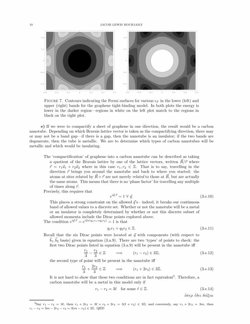
Figure 6. Energy bands calculated for graphene: the bands are shown separately onthe right and left, and shown together in the middle. Notice there are precisely sixdegeneracies located in the firs Brillouin zone.

We see that degeneracy implies that the above discriminant vanishes. This will be thecase if

eiπ(2q2−q1) cos (πq1) = −1

2. (3.a.8)

At first glance, there are two possibilities we may try: first, we know that eiπ(2q2−q1) ∈R, so it must be ±1. If eiπ(2q2−q1) = 1 then 2q2−q1 = 2n for n ∈ Z; the equation aboverequires cos(πq1) = − 1

2 , which means that q1 = 23 or 4

3 . This gives us an infinite classof degenerate solutions, and by adding and subtracting reciprocal lattice vectors, wefind six, essentially equivalent degeneracies at the corners of the first Brillouin zone:

(

1

3,−1

3

) (

−1

3,1

3

) (

1

3,2

3

) (

2

3,1

3

) (

−2

3,−1

3

) (

−1

3,−2

3

)

, (3.a.9)

where the components refer to the values of q1, q2 in ~q = q1~b1 + q2~b2. Now, be-cause adding and subtracting lattice vectors brought us into the other condition fordegeneracy—with 2q2−q1 an odd integer—we know that all of the degeneracies havebeen accounted for.

The energy bands are plotted in Figure 6, where the six degenerate points are clearlyvisible.

c-d) Describe and sketch the topology for various Fermi surfaces that can occur as the filling ofbands is varied. We should also describe the Fermi surface when the lower band is completely filled.

For very low ǫF , the fermi surface is a circle inscribed within the bowl seen in Figure 6.As the energy increases, the Fermi surface appears more and more hexagonal untilfinally it breaks into six arcs—one about each of the corners of the first Brillouinzone. These six regions shrink as ǫF → ǫ0, when they vanish. This is shown inFigure 7.

As ǫF grows above ǫ0, the Fermi surface lies on the upper band and progresses in reverseof the lower-band: for low energies above ǫ0, the Fermi surface is composed of sixdistinct circular components which grow until they become nearly hexagonal; athigh energies, the Fermi surface again approaches a single circular section. Thisprogression is also shown in Figure 7.

In the case when the lower band is completely full, the Fermi ‘surface’ is the union ofthe six distinct Dirac points (of course, only two of them are inequivalent).


-0.6 -0.4 -0.2 0 0.2 0.4 0.6

-0.4

-0.2

0

0.2

0.4

-0.6 -0.4 -0.2 0 0.2 0.4 0.6

-0.4

-0.2

0

0.2

0.4

Figure 7. Contours indicating the Fermi surfaces for various ǫF in the lower (left) andupper (right) bands for the graphene tight-binding model. In both plots the energy islower in the darker region—regions in white on the left plot match to the regions inblack on the right plot.

e) If we were to compactify a sheet of graphene in one direction, the result would be a carbonnanotube. Depending on which Bravais lattice vector is taken as the compactifying direction, there mayor may not be a band gap—if there is a gap, then the nanotube is an insulator; if the two bands aredegenerate, then the tube is metallic. We are to determine which types of carbon nanotubes will bemetallic and which would be insulating.

The ‘compactification’ of graphene into a carbon nanotube can be described as taking

a quotient of the Bravais lattice by one of the lattice vectors, written ~R/~r where~r = r1~a1 + r2~a2 where in this case r1, r2 ∈ Z. That is to say, travelling in thedirection ~r brings you around the nanotube and back to where you started: the

atoms at sites related by ~R+~r are not merely related to those at ~R, but are actuallythe same atoms. This means that there is no ‘phase factor’ for travelling any multipleof times along ~r.

Precisely, this requires thatei~q·~r = 1 ∀ ~q. (3.e.10)

This places a strong constraint on the allowed ~q’s—indeed, it breaks our continuousband of allowed values to a discrete set. Whether or not the nanotube will be a metalor an insulator is completely determined by whether or not this discrete subset ofallowed momenta include the Dirac points explored above.

The condition ei~q·~r = ei2π(q1r1+q2r2) = 1 is that

q1r1 + q2r2 ∈ Z. (3.e.11)

Recall that the six Dirac points were located at ~q with components (with respect to~b1,~b2 basis) given in equation (3.a.9). There are two ‘types’ of points to check: thefirst two Dirac points listed in equation (3.a.9) will be present in the nanotube iff

r13

− r23

∈ Z =⇒ (r1 − r2) ∈ 3Z; (3.e.12)

the second type of point will be present in the nanotube iff

r13

+2r23

∈ Z =⇒ (r1 + 2r2) ∈ 3Z. (3.e.13)

It is not hard to show that these two conditions are in fact equivalent5. Therefore, acarbon nanotube will be a metal in this model only if

r1 − r2 = 3ℓ for some ℓ ∈ Z. (3.e.14)

‘oπǫρ ’ǫδǫι δǫ�ιξαι

5Say r1 − r2 = 3ℓ, then r1 + 2r2 = 3ℓ + r2 + 2r2 = 3(ℓ + r2) ∈ 3Z; and conversely, say r1 + 2r2 = 3m, thenr1 − r2 = 3m − 2r2 − r2 = 3(m − r2) ∈ 3Z. QED


Problem 4: Thermodynamics Near a Dirac PointLet us return our attention to the tight-binding model of graphene from problem 3. We may for the

sake of convenience take ǫ0 = 0.a) The points where two bands become degenerate are called ‘Dirac points.’ We are to determine the

low-temperature behaviour of the specific heat and magnetic spin susceptibility near the Dirac point forgraphene.

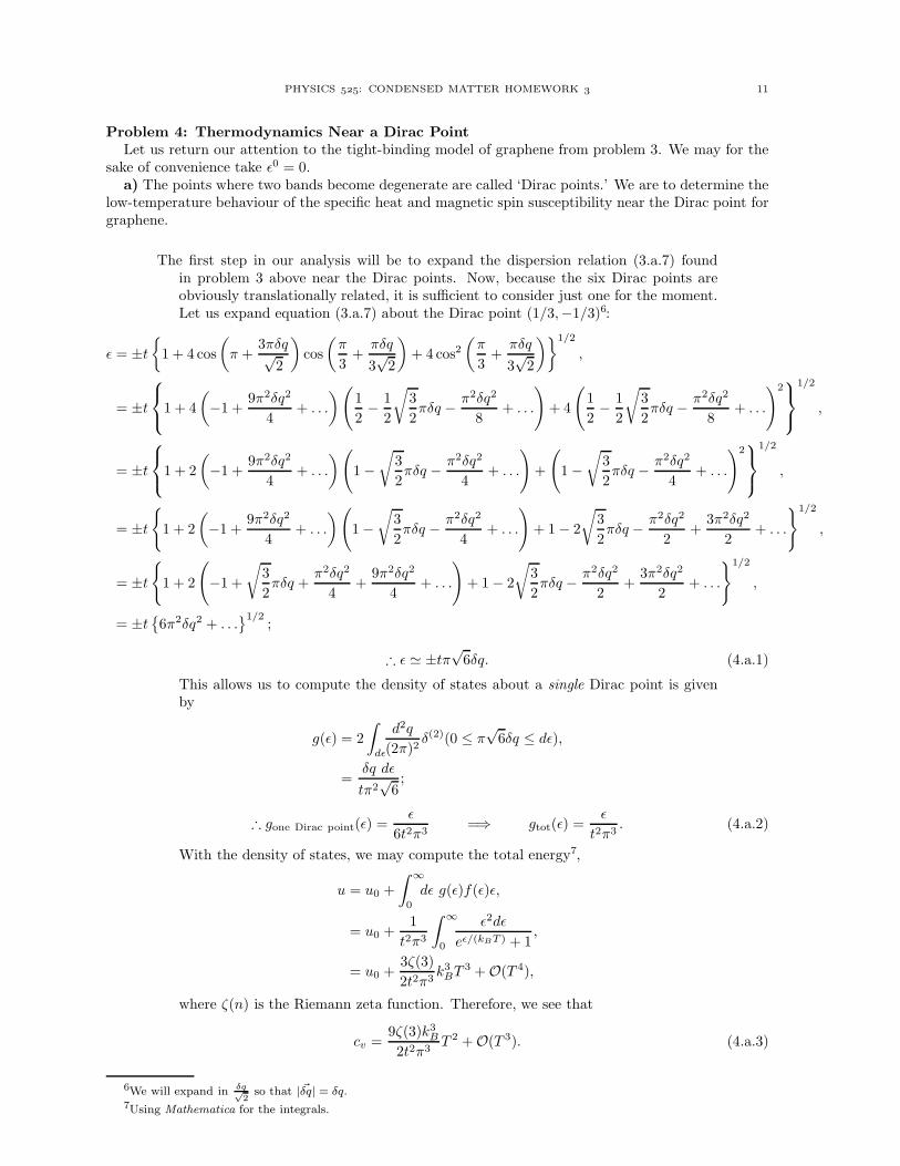
The first step in our analysis will be to expand the dispersion relation (3.a.7) foundin problem 3 above near the Dirac points. Now, because the six Dirac points areobviously translationally related, it is sufficient to consider just one for the moment.Let us expand equation (3.a.7) about the Dirac point (1/3,−1/3)6:

ǫ = ±t{

1 + 4 cos

(

π +3πδq√

2

)

cos

(

π

3+πδq

3√

2

)

+ 4 cos2(

π

3+πδq

3√

2

)}1/2

,

= ±t

1 + 4

(

−1 +9π2δq2

4+ . . .

)

(

1

2− 1

2

√

3

2πδq − π2δq2

8+ . . .

)

+ 4

(

1

2− 1

2

√

3

2πδq − π2δq2

8+ . . .

)2

1/2

,

= ±t

1 + 2

(

−1 +9π2δq2

4+ . . .

)

(

1 −√

3

2πδq − π2δq2

4+ . . .

)

+

(

1 −√

3

2πδq − π2δq2

4+ . . .

)2

1/2

,

= ±t{

1 + 2

(

−1 +9π2δq2

4+ . . .

)

(

1 −√

3

2πδq − π2δq2

4+ . . .

)

+ 1 − 2

√

3

2πδq − π2δq2

2+

3π2δq2

2+ . . .

}1/2

,

= ±t{

1 + 2

(

−1 +

√

3

2πδq +

π2δq2

4+

9π2δq2

4+ . . .

)

+ 1 − 2

√

3

2πδq − π2δq2

2+

3π2δq2

2+ . . .

}1/2

,

= ±t{

6π2δq2 + . . .}1/2

;

∴ ǫ ≃ ±tπ√

6δq. (4.a.1)

This allows us to compute the density of states about a single Dirac point is givenby

g(ǫ) = 2

∫

dǫ

d2q

(2π)2δ(2)(0 ≤ π

√6δq ≤ dǫ),

=δq dǫ

tπ2√

6;

∴ gone Dirac point(ǫ) =ǫ

6t2π3=⇒ gtot(ǫ) =

ǫ

t2π3. (4.a.2)

With the density of states, we may compute the total energy7,

u = u0 +

∫ ∞

0

dǫ g(ǫ)f(ǫ)ǫ,

= u0 +1

t2π3

∫ ∞

0

ǫ2dǫ

eǫ/(kBT ) + 1,

= u0 +3ζ(3)

2t2π3k3

BT3 + O(T 4),

where ζ(n) is the Riemann zeta function. Therefore, we see that

cv =9ζ(3)k3

B

2t2π3T 2 + O(T 3). (4.a.3)

6We will expand in δq√

2so that | ~δq| = δq.

7Using Mathematica for the integrals.


To find the magnetic susceptibility we will begin by referring to the textbook or classnotes wherein it is found that the total magnetization (in the Pauli model) is givenby

M = µ2H

∫

dǫ g′(ǫ)f(ǫ). (4.a.4)

Evaluating this integral directly, we see

χ =∂M

∂H= µ2 kBT log(2)

t2π3+ O(T 2). (4.a.5)

b) Consider doping graphene so that ǫF is just above the Dirac point, but by an amount much lessthat of T ; we are to again describe the low-temperature approximations of the specific heat and magneticspin susceptibility.

I am pretty sure that the picture we are supposed to envision is that we are some ǫFseparated from the Dirac point, yet close enough to it that g(ǫ) can be still viewedas a linear function of ǫ. If this is the appropriate, then we can take

g(ǫ) =ǫ− ǫFt2π3

and f(ǫ) =1

e(ǫ−ǫf)/(kBT ) + 1,

and integrate above the Fermi surface8. Using a computer algebra package, we find

u = u0 +1

t2π3

∫ ∞

ǫF

ǫ(ǫ− ǫF ) dǫ

e(ǫ−ǫF )/(kBT ) + 1,

=ǫFk

2B

12t2πT 2 +

3ζ(3)k3B

2t2π3T 3 + O(T 4).

(It is comforting that this reproduces our earlier result for vanishing ǫF .) This allowsus to directly conclude that

∴ cv =ǫFk

2B

6t2πT +

9ζ(3)k3B

2t2π3T 2 + O(T 3). (4.b.1)

Now, to find the magnetic susceptibility, we perform the same steps as before and see

M = µ2H

∫

dǫ g(ǫ)f(ǫ) = µ2H1

t2π3

(

kBT log(2) +ǫF2

)

, (4.b.2)

and so

∴ χ = µ2 1

t2π3

(

kBT log(2) +eF

2

)

. (4.b.3)

8There are alternative ways of looking at this.

Documents

Homework 3