Embed Size (px)
Citation preview
HOW SMOOTH IS YOUR WAVELET? WAVELET
REGULARITY VIA THERMODYNAMIC FORMALISM
M. Pollicott and H. Weiss
June 9, 2005 9:49am
Abstract. A popular wavelet reference [W] states that “in theoretical and practical studies,the notion of (wavelet) regularity has been increasing in importance.” Not surprisingly, the
study of wavelet regularity is currently a major topic of investigation. Smoother wavelets
provide sharper frequency resolution of functions. Also, the iterative algorithms to constructwavelets converge faster for smoother wavelets. The main goals of this paper are to extend,
refine, and unify the thermodynamic approach to the regularity of wavelets and to devise afaster algorithm for estimating regularity.
We present an algorithm for computing the Sobolev regularity of wavelets and prove that
it converges with super-exponential speed. As an application we construct new examples ofwavelets that are smoother than the Daubechies wavelets and have the same support. We
establish smooth dependence of the regularity for wavelet families, and we derive a variational
formula for the regularity. We also show a general relation between the asymptotic regularityof wavelet families and maximal measures for the doubling map. Finally, we describe how
these results generalize to higher dimensional wavelets.
0. Introduction
While the Fourier transform is useful for analyzing stationary functions, it is much lessuseful for analyzing non-stationary cases, where the frequency content evolves over time. Inmany applications one needs to estimate the frequency content of a nonstationary functionlocally in time, for example, to determine when a transient event occurred. This mightarise from a sudden computer fan failure or from a pop on a music compact disk. Theusual Fourier transform does not provide simultaneous time and frequency localization ofa function.
The windowed or short-time Fourier transform does provide simultaneous time andfrequency localization. However, since it uses a fixed time window width, the same windowwidth is used over the entire frequency domain. In applications, a fixed window width isfrequently unnecessarily large for a signal having strong high frequency components andunnecessarily small for a signal having strong low frequency components.
In contrast, the wavelet transform provides a decomposition of a function into compo-nents from different scales whose degree of localization is connected to the size of the scale
Typeset by AMS-TEX
1
2 M. POLLICOTT AND H. WEISS
window. This is achieved by integer translations and dyadic dilations of a single function:the wavelet.
The special class of orthogonal wavelets are those for which the translations and dilationsof a fixed function, say, ψ form an orthonormal basis of L2(R). Examples include Haarwavelet, Shannon wavelet, Meyer wavelet, Battle-Lemari wavelets, Daubechies wavelets,and Coiffman wavelets. A standard way to construct an orthogonal wavelet is to solve thedilation equation
φ(x) =√
2∞∑
k=−∞
ckφ(2x− k), (0.1)
with the normalization∑
k ck = 1. Very few solutions of the dilation equation for waveletsare known to have closed form expressions. This is one reason why it is difficult to de-termine the regularity of wavelets.1 Provided the solution φ satisfies some additionalconditions, the function ψ defined by
ψ(x) =∞∑
n=−∞(−1)kc1−kφ(2x− k),
is an orthogonal wavelet, i.e., the set {2j/2ψ(2jx− n) : j, n ∈ Z} is an orthonormal basisfor L2(R). Henceforth, the term wavelet will mean orthogonal wavelet.
Daubechies [Da1] made the breakthrough of constructing smoother compactly supportedwavelets. For these wavelets, the wavelet coefficients {ck} satisfy simple recursion relations,and thus can be quickly computed. However, the Daubechies wavelets necessarily possessonly finite smoothness.2 Smoother wavelets provide sharper frequency resolution of func-tions. Also, the regularity of the wavelet determines the speed of convergence of the cascadealgorithm [Da1], which is another standard method to construct the wavelet from equation(0.1). Thus knowing the smoothness or regularity of wavelets has important practical andtheoretical consequences.
The main goals of this paper are to extend, refine, and unify the thermodynamic approachto the regularity of wavelets and to devise a faster algorithm for estimating regularity.
In Section 1 we recall the construction of wavelets using multiresolution analysis. Wethen discuss how the Lp-Sobolev regularity of wavelets is related to the thermodynamicpressure of the doubling map E2 : [0, 2π) → [0, 2π). The latter is the crucial link betweenwavelets and dynamical systems.
Previous authors have noted that for compactly supported wavelets, the transfer op-erator preserves a finite dimensional subspace and is thus represented by a d × d matrix.Providing the matrix is small, its maximal eigenvalue, which is related to the pressure, canbe explicitly computed, and thus the Lp-Sobolev regularity can be determined by matrixalgebra.
1We learned in [Da2] (see references) that this dilation equation arises in other areas, including sub-
division schemes for computer aided design, where the goal is the fast generation of smooth curves andsurface.
2Frequently, increasing the support of the function leads to increased smoothness.
HOW SMOOTH IS YOUR WAVELET? 3
Cohen and Daubechies identified the Lp-Sobolev regularity in terms of the smallest zeroof the Fredholm-Ruelle determinant for the transfer operator acting on a certain Hilbertspace of analytic functions [CD1, Da2]. Their analysis leads to an algorithm for the Sobolevregularity of wavelets having analytic filters that converges with exponential speed. InSection 2, we study the transfer operator acting on the Bergman space of analytic functionsand effect a more refined analysis. This leads to a more efficient algorithm which convergeswith super-exponential speed to the Lp-Sobolev regularity of the wavelet. The algorithminvolves computing certain orbital averages over the periodic points of the doubling mapE2.
In Section 3 we illustrate, in a number of examples, the advantage of this methodover the earlier Cohen-Daubechies method. Running on a fast desktop computer, thisalgorithm provides a highly accurate approximation for the Sobolev regularity in less thantwo minutes.
A feature of this thermodynamic approach is that it works equally well for compactlysupported and non-compactly supported wavelets (e.g., Butterworth filters). In practice,for wavelets with large support, the distinction may become immaterial, and the use ofour algorithm which applies to arbitrary wavelets may prove quite useful.
In Section 4, we use this improved algorithm to study the parameter dependence of theLp-Sobolev regularity in several smooth families of wavelets. In particular, we constructnew examples of wavelets having the same support as Daubechies wavelets, but with higherregularity.
In Section 5, we show that the Lp-Sobolev regularity depends smoothly on the wavelet,and we provide, via thermodynamic formalism, a variational formula. This problem hasbeen considered experimentally by Daubechies [Da1] and Ojanen [Oj1] for different param-eterized families. Our thermodynamic approach, based on properties of pressure, gives asound theoretical foundation for this analysis.
In Section 6, we study the asymptotic behavior of the Lp-Sobolev regularity of waveletfamilies. We establish a general relation between this asymptotic regularity and maximalmeasures for the doubling map, extending work of Cohen and Conze [CC1]. The study ofmaximal measures is currently an active research area in dynamical systems.
In Section 7, we describe the natural generalization of these results to arbitrary dimen-sions.
Finally, in Section 8, we briefly describe the natural generalization of these results towavelets whose filters are not analytic.
1. Wavelets: construction and regularity
Constructing Wavelets. We begin by recalling the construction of wavelets via mul-tiresolution analysis. A comprehensive reference for wavelets is [Da1], which also containsan extensive bibliography.
The Fourier transform of the scaling equation (0.1) satisfies
φ(ξ) = m(ξ/2)φ(ξ/2), where m(ξ) =1√2
∑k
cke−ikξ. (1.1)
4 M. POLLICOTT AND H. WEISS
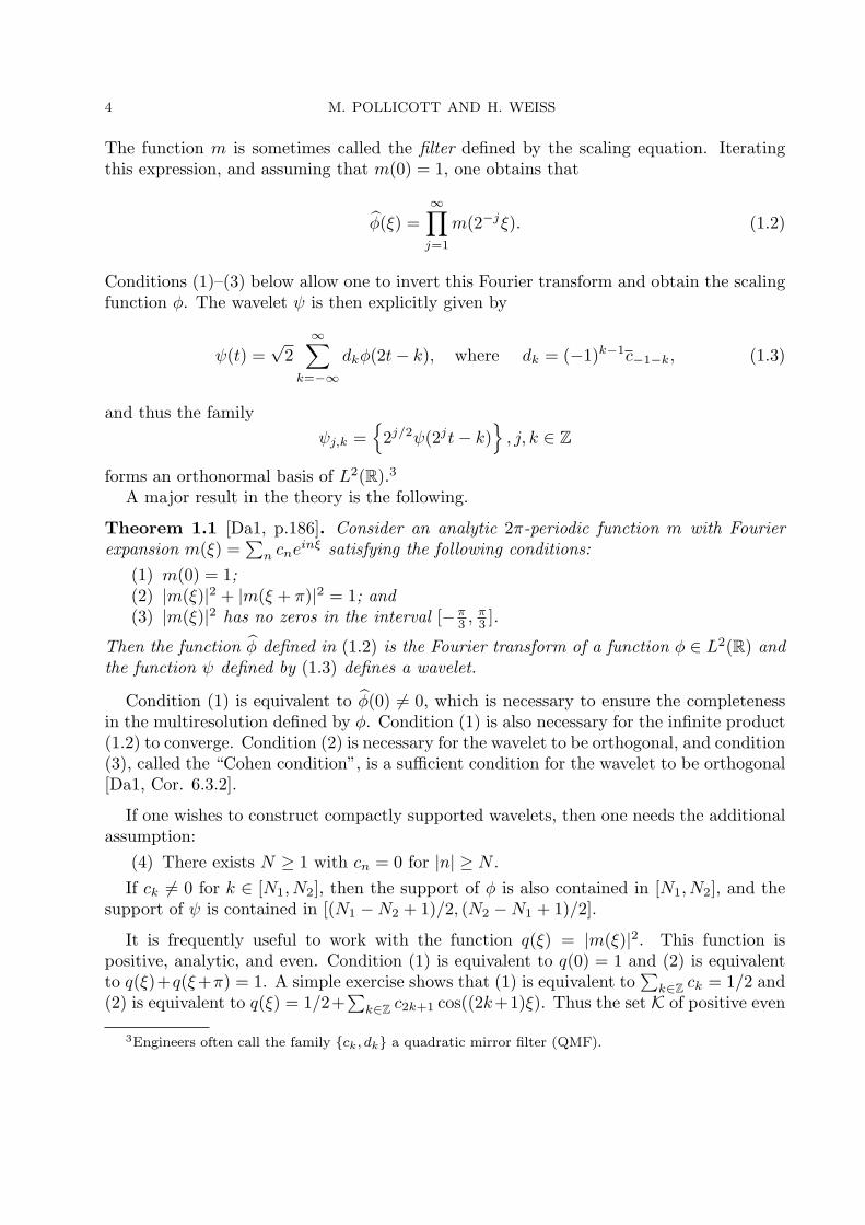
The function m is sometimes called the filter defined by the scaling equation. Iteratingthis expression, and assuming that m(0) = 1, one obtains that
φ(ξ) =∞∏
j=1
m(2−jξ). (1.2)
Conditions (1)–(3) below allow one to invert this Fourier transform and obtain the scalingfunction φ. The wavelet ψ is then explicitly given by
ψ(t) =√
2∞∑
k=−∞
dkφ(2t− k), where dk = (−1)k−1c−1−k, (1.3)
and thus the familyψj,k =
{2j/2ψ(2jt− k)
}, j, k ∈ Z
forms an orthonormal basis of L2(R).3
A major result in the theory is the following.
Theorem 1.1 [Da1, p.186]. Consider an analytic 2π-periodic function m with Fourierexpansion m(ξ) =
∑n cne
inξ satisfying the following conditions:(1) m(0) = 1;(2) |m(ξ)|2 + |m(ξ + π)|2 = 1; and(3) |m(ξ)|2 has no zeros in the interval [−π
3 ,π3 ].
Then the function φ defined in (1.2) is the Fourier transform of a function φ ∈ L2(R) andthe function ψ defined by (1.3) defines a wavelet.
Condition (1) is equivalent to φ(0) 6= 0, which is necessary to ensure the completenessin the multiresolution defined by φ. Condition (1) is also necessary for the infinite product(1.2) to converge. Condition (2) is necessary for the wavelet to be orthogonal, and condition(3), called the “Cohen condition”, is a sufficient condition for the wavelet to be orthogonal[Da1, Cor. 6.3.2].
If one wishes to construct compactly supported wavelets, then one needs the additionalassumption:
(4) There exists N ≥ 1 with cn = 0 for |n| ≥ N .If ck 6= 0 for k ∈ [N1, N2], then the support of φ is also contained in [N1, N2], and the
support of ψ is contained in [(N1 −N2 + 1)/2, (N2 −N1 + 1)/2].
It is frequently useful to work with the function q(ξ) = |m(ξ)|2. This function ispositive, analytic, and even. Condition (1) is equivalent to q(0) = 1 and (2) is equivalentto q(ξ)+q(ξ+π) = 1. A simple exercise shows that (1) is equivalent to
∑k∈Z ck = 1/2 and
(2) is equivalent to q(ξ) = 1/2+∑
k∈Z c2k+1 cos((2k+1)ξ). Thus the set K of positive even
3Engineers often call the family {ck, dk} a quadratic mirror filter (QMF).
HOW SMOOTH IS YOUR WAVELET? 5
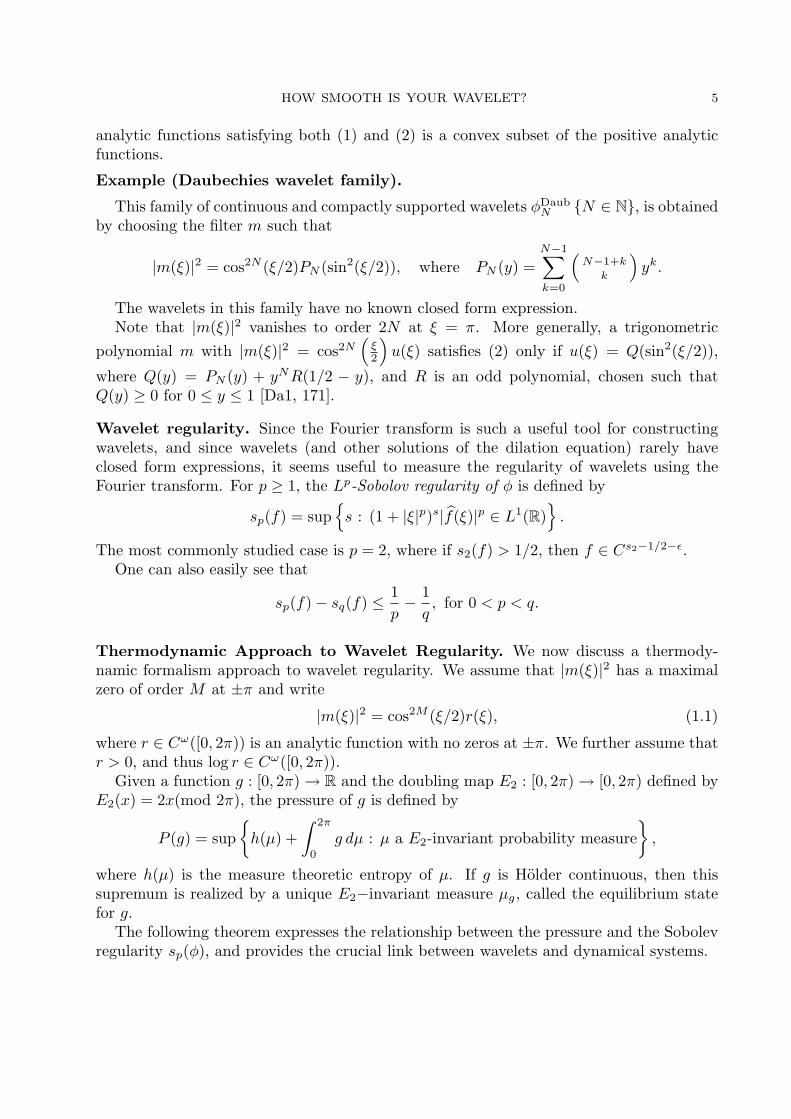
analytic functions satisfying both (1) and (2) is a convex subset of the positive analyticfunctions.
Example (Daubechies wavelet family).
This family of continuous and compactly supported wavelets φDaubN {N ∈ N}, is obtained
by choosing the filter m such that
|m(ξ)|2 = cos2N (ξ/2)PN (sin2(ξ/2)), where PN (y) =N−1∑k=0
(N−1+k
k
)yk.
The wavelets in this family have no known closed form expression.Note that |m(ξ)|2 vanishes to order 2N at ξ = π. More generally, a trigonometric
polynomial m with |m(ξ)|2 = cos2N(
ξ2
)u(ξ) satisfies (2) only if u(ξ) = Q(sin2(ξ/2)),
where Q(y) = PN (y) + yNR(1/2 − y), and R is an odd polynomial, chosen such thatQ(y) ≥ 0 for 0 ≤ y ≤ 1 [Da1, 171].
Wavelet regularity. Since the Fourier transform is such a useful tool for constructingwavelets, and since wavelets (and other solutions of the dilation equation) rarely haveclosed form expressions, it seems useful to measure the regularity of wavelets using theFourier transform. For p ≥ 1, the Lp-Sobolov regularity of φ is defined by
sp(f) = sup{s : (1 + |ξ|p)s|f(ξ)|p ∈ L1(R)
}.
The most commonly studied case is p = 2, where if s2(f) > 1/2, then f ∈ Cs2−1/2−ε.One can also easily see that
sp(f)− sq(f) ≤ 1p− 1q, for 0 < p < q.
Thermodynamic Approach to Wavelet Regularity. We now discuss a thermody-namic formalism approach to wavelet regularity. We assume that |m(ξ)|2 has a maximalzero of order M at ±π and write
|m(ξ)|2 = cos2M (ξ/2)r(ξ), (1.1)
where r ∈ Cω([0, 2π)) is an analytic function with no zeros at ±π. We further assume thatr > 0, and thus log r ∈ Cω([0, 2π)).
Given a function g : [0, 2π) → R and the doubling map E2 : [0, 2π) → [0, 2π) defined byE2(x) = 2x(mod 2π), the pressure of g is defined by
P (g) = sup{h(µ) +
∫ 2π
0
g dµ : µ a E2-invariant probability measure},
where h(µ) is the measure theoretic entropy of µ. If g is Holder continuous, then thissupremum is realized by a unique E2−invariant measure µg, called the equilibrium statefor g.
The following theorem expresses the relationship between the pressure and the Sobolevregularity sp(φ), and provides the crucial link between wavelets and dynamical systems.
6 M. POLLICOTT AND H. WEISS
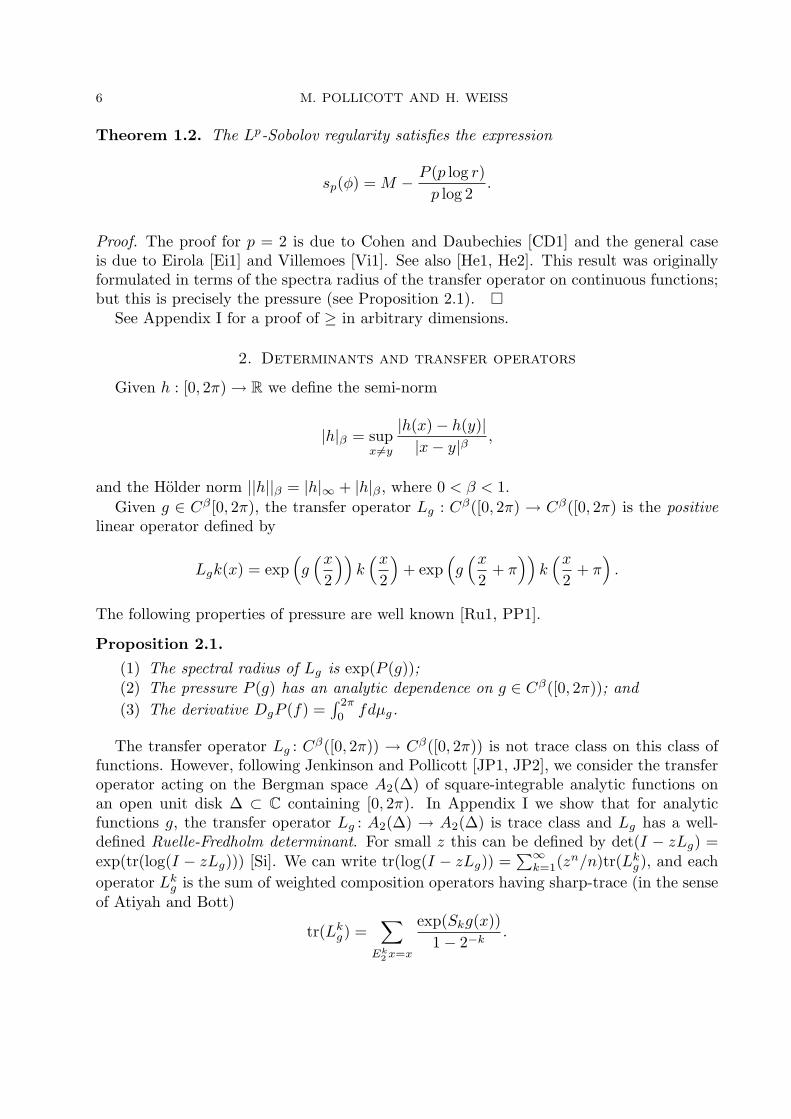
Theorem 1.2. The Lp-Sobolov regularity satisfies the expression
sp(φ) = M − P (p log r)p log 2
.
Proof. The proof for p = 2 is due to Cohen and Daubechies [CD1] and the general caseis due to Eirola [Ei1] and Villemoes [Vi1]. See also [He1, He2]. This result was originallyformulated in terms of the spectra radius of the transfer operator on continuous functions;but this is precisely the pressure (see Proposition 2.1). �
See Appendix I for a proof of ≥ in arbitrary dimensions.
2. Determinants and transfer operators
Given h : [0, 2π) → R we define the semi-norm
|h|β = supx6=y
|h(x)− h(y)||x− y|β
,
and the Holder norm ||h||β = |h|∞ + |h|β , where 0 < β < 1.Given g ∈ Cβ [0, 2π), the transfer operator Lg : Cβ([0, 2π) → Cβ([0, 2π) is the positive
linear operator defined by
Lgk(x) = exp(g(x
2
))k(x
2
)+ exp
(g(x
2+ π
))k(x
2+ π
).
The following properties of pressure are well known [Ru1, PP1].
Proposition 2.1.
(1) The spectral radius of Lg is exp(P (g));(2) The pressure P (g) has an analytic dependence on g ∈ Cβ([0, 2π)); and(3) The derivative DgP (f) =
∫ 2π
0fdµg.
The transfer operator Lg : Cβ([0, 2π)) → Cβ([0, 2π)) is not trace class on this class offunctions. However, following Jenkinson and Pollicott [JP1, JP2], we consider the transferoperator acting on the Bergman space A2(∆) of square-integrable analytic functions onan open unit disk ∆ ⊂ C containing [0, 2π). In Appendix I we show that for analyticfunctions g, the transfer operator Lg : A2(∆) → A2(∆) is trace class and Lg has a well-defined Ruelle-Fredholm determinant. For small z this can be defined by det(I − zLg) =exp(tr(log(I − zLg))) [Si]. We can write tr(log(I − zLg)) =
∑∞k=1(zn/n)tr(Lk
g), and eachoperator Lk
g is the sum of weighted composition operators having sharp-trace (in the senseof Atiyah and Bott)
tr(Lkg) =
∑Ek
2 x=x
exp(Skg(x))1− 2−k
.
HOW SMOOTH IS YOUR WAVELET? 7
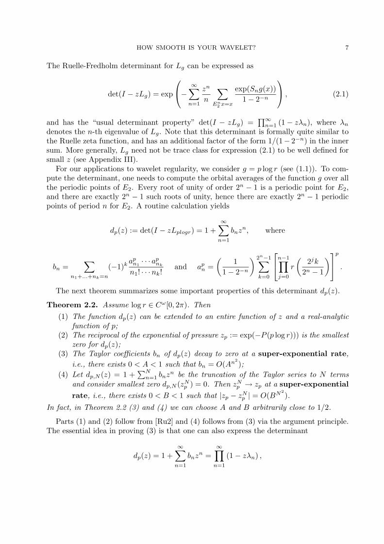
The Ruelle-Fredholm determinant for Lg can be expressed as
det(I − zLg) = exp
− ∞∑n=1
zn
n
∑En
2 x=x
exp(Sng(x))1− 2−n
, (2.1)
and has the “usual determinant property” det(I − zLg) =∏∞
n=1 (1− zλn), where λn
denotes the n-th eigenvalue of Lg. Note that this determinant is formally quite similar tothe Ruelle zeta function, and has an additional factor of the form 1/(1− 2−n) in the innersum. More generally, Lg need not be trace class for expression (2.1) to be well defined forsmall z (see Appendix III).
For our applications to wavelet regularity, we consider g = p log r (see (1.1)). To com-pute the determinant, one needs to compute the orbital averages of the function g over allthe periodic points of E2. Every root of unity of order 2n − 1 is a periodic point for E2,and there are exactly 2n − 1 such roots of unity, hence there are exactly 2n − 1 periodicpoints of period n for E2. A routine calculation yields
dp(z) := det(I − zLplogr) = 1 +∞∑
n=1
bnzn, where
bn =∑
n1+...+nk=n
(−1)k apn1· · · ap
nk
n1! · · ·nk!and ap
n =(
11− 2−n
) 2n−1∑k=0
n−1∏j=0
r
(2jk
2n − 1
)p
.
The next theorem summarizes some important properties of this determinant dp(z).
Theorem 2.2. Assume log r ∈ Cω[0, 2π). Then(1) The function dp(z) can be extended to an entire function of z and a real-analytic
function of p;(2) The reciprocal of the exponential of pressure zp := exp(−P (p log r))) is the smallest
zero for dp(z);(3) The Taylor coefficients bn of dp(z) decay to zero at a super-exponential rate,
i.e., there exists 0 < A < 1 such that bn = O(An2);
(4) Let dp,N (z) = 1 +∑N
n=1 bnzn be the truncation of the Taylor series to N terms
and consider smallest zero dp,N (zNp ) = 0. Then zN
p → zp at a super-exponentialrate, i.e., there exists 0 < B < 1 such that |zp − zN
p | = O(BN2).
In fact, in Theorem 2.2 (3) and (4) we can choose A and B arbitrarily close to 1/2.
Parts (1) and (2) follow from [Ru2] and (4) follows from (3) via the argument principle.The essential idea in proving (3) is that one can also express the determinant
dp(z) = 1 +∞∑
n=1
bnzn =
∞∏n=1
(1− zλn) ,
8 M. POLLICOTT AND H. WEISS
where λn denotes the n-th eigenvalue of Lp log r [Sim]. It follows that the coefficient bn =∑i1<···<in
λi1 · · ·λin. To show that the Taylor coefficients have super exponential decay,
it suffices to show a suitable estimate on the eigenvalues. We present a proof in AppendixI.
Part (4) of this theorem provides an algorithm for computing the Sobolevregularity which converges with super-exponential speed in N . The calculationof dp,N (z) for N = 12 takes less than two minutes on a desktop computer.
For our applications to wavelets, we shall take either g = log |m|2 or g = log r. In fact,both functions lead to equivalent results. The following proposition relates the zeros ofdet(1− zLlog r) and det(1− zL|m|2).4
Proposition 2.3. The determinant det(1− zLlog |m|2) has zeros at
(1) 1, 2, 4, . . . , 2M−1; and(2) 2Mz, where z is a zero for det(1− zLlog r).
This was observed by Cohen and Daubechies [CD1] and we include a short proof inAppendix II.
3. Examples: Computation of Sobolev regularity using the determinant
In this section we shall apply Theorem 2.2 to estimate the Sobolev exponent sp(φ) ofcertain interesting examples.
3.1 Daubechies wavelet family.
Example 1: (N = 3 and p = 2). In this case d2(z) is a polynomial of degree 5 with rationalcoefficients:
d2(z) = 1− 2z − 57.1875z2 − 74.53125z3 + 210.09375z4 − 91.125z5,
which has its first zero at z0 = 0.111 . . . . By Theorem 1.2 we deduce the precise values2(ψDaub
3 ) = 3 + log(0.1111 . . . )/2 log 2 = 1.415037 . . . .5
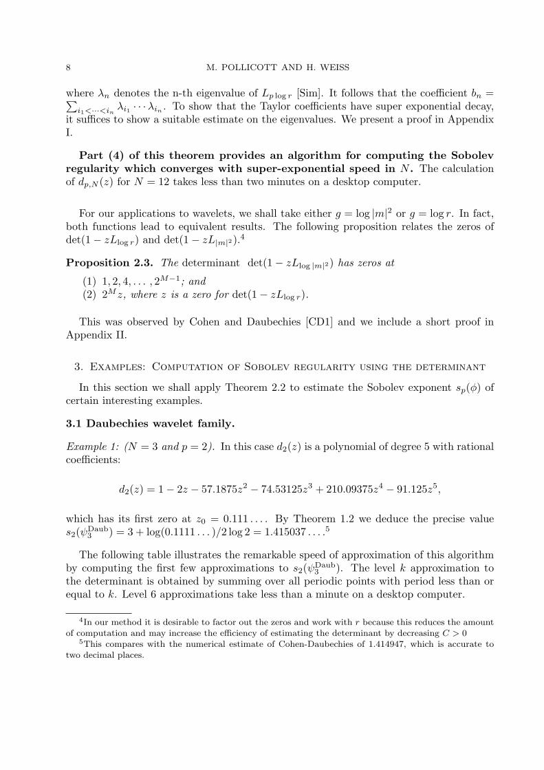
The following table illustrates the remarkable speed of approximation of this algorithmby computing the first few approximations to s2(ψDaub
3 ). The level k approximation tothe determinant is obtained by summing over all periodic points with period less than orequal to k. Level 6 approximations take less than a minute on a desktop computer.
4In our method it is desirable to factor out the zeros and work with r because this reduces the amount
of computation and may increase the efficiency of estimating the determinant by decreasing C > 05This compares with the numerical estimate of Cohen-Daubechies of 1.414947, which is accurate to
two decimal places.
HOW SMOOTH IS YOUR WAVELET? 9
N Smallest root of d2 Approx to s2(ψDaub3 )
1 0.50000000000000000 2.50000000000000002 0.11590073269851241 1.44548079594062973 0.10935186260699924 1.40352484967659804 0.11120565746767627 1.41565104529629385 0.11111111111111109 1.41503749927884376 0.11111111111111111 1.4150374992788437
Example 2: (N = 2 and p = 4). In this case d4(z) is a polynomial of degree 5 with rationalcofficients:
d4(z) = 1− 2z − 50.75z2 − 76.25z3 + 115z4 − 32z5,
which has its first zero at z0 = 0.115146 . . . . By Theorem 2.1 we deduce that s4(ψDaub2 ) =
3 + log(0.115146 . . . )/2 log 2 = 1.22038 . . . .6
Example 3: (N = 4 and p = 2). In this case d2(z) is a polynomial of degree 7 with rationalcoefficients
d2(z) = 1− 2z − 433z2 − 996z3 + 23572z4 − 32288z5 − 68627z6 − 24414z7,
which has its first zero at z0 = 0.045788 . . . . By Theorem 2.1 we deduce that s2(ψDaub4 ) =
4 + log(0.045788 . . . )/2 log 2 = 1.77557 . . . .7
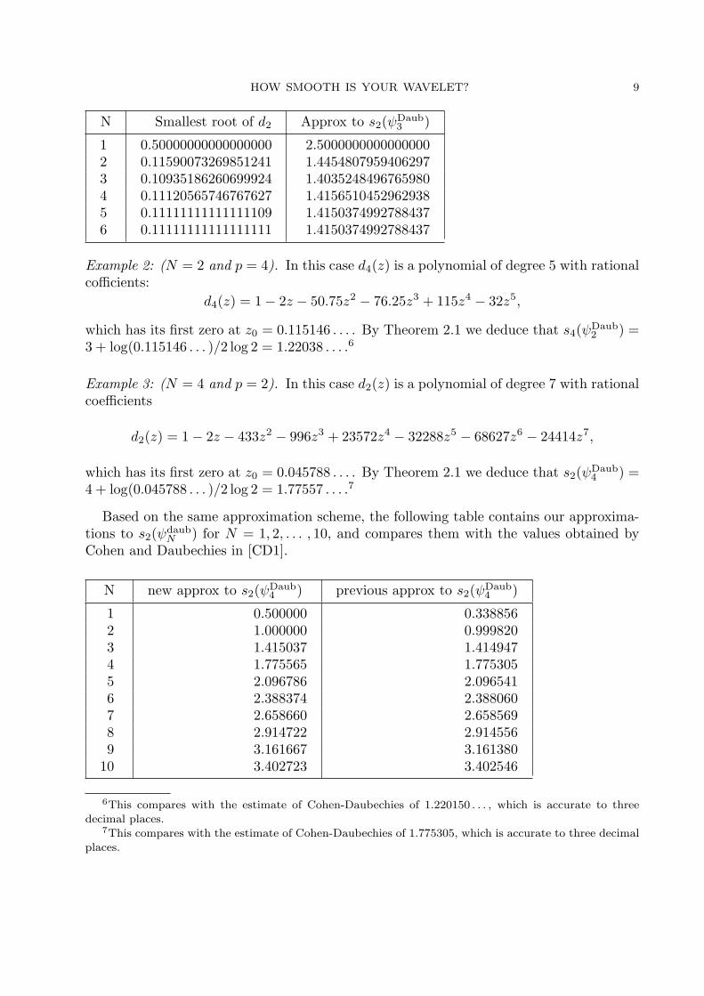
Based on the same approximation scheme, the following table contains our approxima-tions to s2(ψdaub
N ) for N = 1, 2, . . . , 10, and compares them with the values obtained byCohen and Daubechies in [CD1].
N new approx to s2(ψDaub4 ) previous approx to s2(ψDaub
4 )
1 0.500000 0.3388562 1.000000 0.9998203 1.415037 1.4149474 1.775565 1.7753055 2.096786 2.0965416 2.388374 2.3880607 2.658660 2.6585698 2.914722 2.9145569 3.161667 3.161380
10 3.402723 3.402546
6This compares with the estimate of Cohen-Daubechies of 1.220150 . . . , which is accurate to three
decimal places.7This compares with the estimate of Cohen-Daubechies of 1.775305, which is accurate to three decimal
places.
10 M. POLLICOTT AND H. WEISS
Remark. In examples 1 − 3 the determinant is a rational function. This is an immediateconsequence of the fact that the transfer operator preserves the finite dimensional subspaceof functions spanned by
{1, cos(ξ), cos(2ξ), · · · , cos(Nξ)}.
This fact has been observed by several authors, c.f., [Oj1].
3.2 Butterworth filter family.The Butterworth filter is the filter type with flattest pass band and which allows a
moderate group delay [OS1]. These filters form an important family of non-compactlysupported wavelets and are defined by
|m(ξ)|2 =cos2N (ξ/2)
sin2N (ξ/2) + cos2N (ξ/2), N ∈ N.
We suppress the index n for notational convenience. It is easy to check that |m(ξ)|2 satisfiesconditions (1)− (3) on page 4.
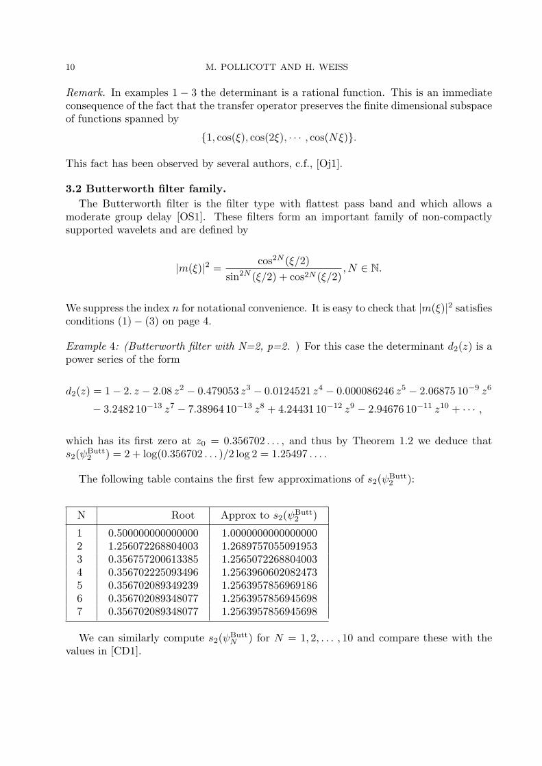
Example 4: (Butterworth filter with N=2, p=2. ) For this case the determinant d2(z) is apower series of the form
d2(z) = 1− 2. z − 2.08 z2 − 0.479053 z3 − 0.0124521 z4 − 0.000086246 z5 − 2.06875 10−9 z6
− 3.2482 10−13 z7 − 7.38964 10−13 z8 + 4.24431 10−12 z9 − 2.94676 10−11 z10 + · · · ,
which has its first zero at z0 = 0.356702 . . . , and thus by Theorem 1.2 we deduce thats2(ψButt
2 ) = 2 + log(0.356702 . . . )/2 log 2 = 1.25497 . . . .
The following table contains the first few approximations of s2(ψButt2 ):
N Root Approx to s2(ψButt2 )
1 0.500000000000000 1.00000000000000002 1.256072268804003 1.26897570550919533 0.356757200613385 1.25650722688040034 0.356702225093496 1.25639606020824735 0.356702089349239 1.25639578569691866 0.356702089348077 1.25639578569456987 0.356702089348077 1.2563957856945698
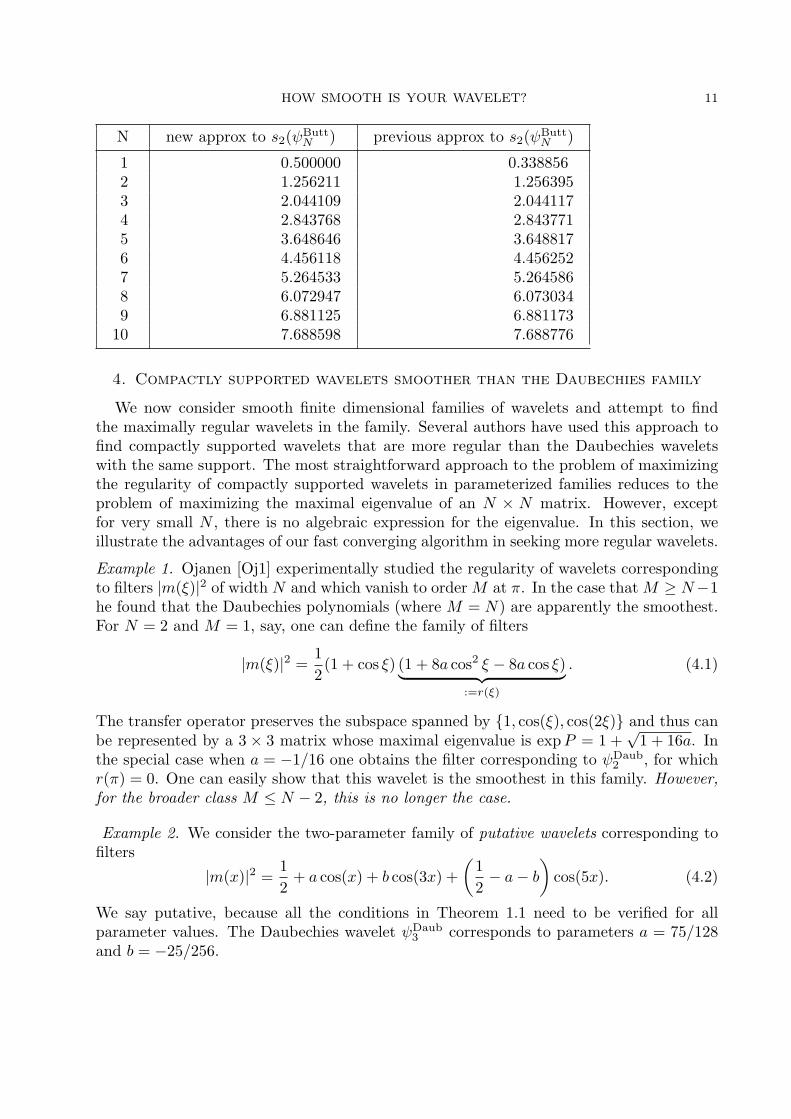
We can similarly compute s2(ψButtN ) for N = 1, 2, . . . , 10 and compare these with the
values in [CD1].
HOW SMOOTH IS YOUR WAVELET? 11
N new approx to s2(ψButtN ) previous approx to s2(ψButt
N )
1 0.500000 0.3388562 1.256211 1.2563953 2.044109 2.0441174 2.843768 2.8437715 3.648646 3.6488176 4.456118 4.4562527 5.264533 5.2645868 6.072947 6.0730349 6.881125 6.881173
10 7.688598 7.688776
4. Compactly supported wavelets smoother than the Daubechies family
We now consider smooth finite dimensional families of wavelets and attempt to findthe maximally regular wavelets in the family. Several authors have used this approach tofind compactly supported wavelets that are more regular than the Daubechies waveletswith the same support. The most straightforward approach to the problem of maximizingthe regularity of compactly supported wavelets in parameterized families reduces to theproblem of maximizing the maximal eigenvalue of an N × N matrix. However, exceptfor very small N , there is no algebraic expression for the eigenvalue. In this section, weillustrate the advantages of our fast converging algorithm in seeking more regular wavelets.
Example 1. Ojanen [Oj1] experimentally studied the regularity of wavelets correspondingto filters |m(ξ)|2 of width N and which vanish to order M at π. In the case that M ≥ N−1he found that the Daubechies polynomials (where M = N) are apparently the smoothest.For N = 2 and M = 1, say, one can define the family of filters
|m(ξ)|2 =12
(1 + cos ξ) (1 + 8a cos2 ξ − 8a cos ξ)︸ ︷︷ ︸:=r(ξ)
. (4.1)
The transfer operator preserves the subspace spanned by {1, cos(ξ), cos(2ξ)} and thus canbe represented by a 3 × 3 matrix whose maximal eigenvalue is expP = 1 +
√1 + 16a. In
the special case when a = −1/16 one obtains the filter corresponding to ψDaub2 , for which
r(π) = 0. One can easily show that this wavelet is the smoothest in this family. However,for the broader class M ≤ N − 2, this is no longer the case.
Example 2. We consider the two-parameter family of putative wavelets corresponding tofilters
|m(x)|2 =12
+ a cos(x) + b cos(3x) +(
12− a− b
)cos(5x). (4.2)
We say putative, because all the conditions in Theorem 1.1 need to be verified for allparameter values. The Daubechies wavelet ψDaub
3 corresponds to parameters a = 75/128and b = −25/256.
12 M. POLLICOTT AND H. WEISS
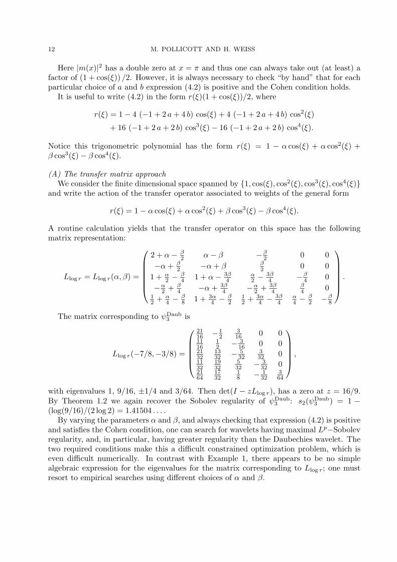
Here |m(x)|2 has a double zero at x = π and thus one can always take out (at least) afactor of (1 + cos(ξ)) /2. However, it is always necessary to check “by hand” that for eachparticular choice of a and b expression (4.2) is positive and the Cohen condition holds.
It is useful to write (4.2) in the form r(ξ)(1 + cos(ξ))/2, where
r(ξ) = 1− 4 (−1 + 2 a+ 4 b) cos(ξ) + 4 (−1 + 2 a+ 4 b) cos2(ξ)
+ 16 (−1 + 2 a+ 2 b) cos3(ξ)− 16 (−1 + 2 a+ 2 b) cos4(ξ).
Notice this trigonometric polynomial has the form r(ξ) = 1 − α cos(ξ) + α cos2(ξ) +β cos3(ξ)− β cos4(ξ).
(A) The transfer matrix approachWe consider the finite dimensional space spanned by {1, cos(ξ), cos2(ξ), cos3(ξ), cos4(ξ)}
and write the action of the transfer operator associated to weights of the general form
r(ξ) = 1− α cos(ξ) + α cos2(ξ) + β cos3(ξ)− β cos4(ξ).
A routine calculation yields that the transfer operator on this space has the followingmatrix representation:
Llog r = Llog r(α, β) =
2 + α− β
2 α− β −β2 0 0
−α+ β2 −α+ β β
2 0 01 + α
2 −β4 1 + α− 3β
4α2 −
3β4 −β
4 0−α
2 + β4 −α+ 3β
4 −α2 + 3β
4β4 0
12 + α
4 −β8 1 + 3α
4 − β2
12 + 3α
4 − 3β4
α4 −
β2 −β
8
.
The matrix corresponding to ψDaub3 is
Llog r(−7/8,−3/8) =
2116 − 1
2316 0 0
1116
12 − 3
16 0 02132
1332 − 5
32332 0
1132
1932
532 − 3
32 02164
1732
18 − 1
32364
,
with eigenvalues 1, 9/16, ±1/4 and 3/64. Then det(I − zLlog r), has a zero at z = 16/9.By Theorem 1.2 we again recover the Sobolev regularity of ψDaub
3 : s2(ψDaub3 ) = 1 −
(log(9/16)/(2 log 2) = 1.41504 . . . .By varying the parameters α and β, and always checking that expression (4.2) is positive
and satisfies the Cohen condition, one can search for wavelets having maximal Lp−Sobolevregularity, and, in particular, having greater regularity than the Daubechies wavelet. Thetwo required conditions make this a difficult constrained optimization problem, which iseven difficult numerically. In contrast with Example 1, there appears to be no simplealgebraic expression for the eigenvalues for the matrix corresponding to Llog r; one mustresort to empirical searches using different choices of α and β.
HOW SMOOTH IS YOUR WAVELET? 13
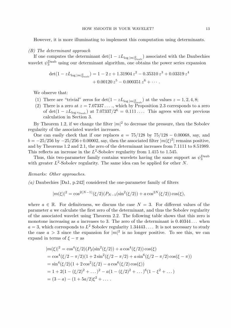
However, it is more illuminating to implement this computation using determinants.
(B) The determinant approachIf one computes the determinant det(1− zLlog |m|2Daub
) associated with the Daubechieswavelet ψDaub
3 using our determinant algorithm, one obtains the power series expansion
det(1− zLlog |m|2Daub) = 1− 2 z + 1.31904 z2 − 0.35310 z3 + 0.03319 z4
+ 0.00120 z5 − 0.000351 z6 + · · · .
We observe that:(1) There are “trivial” zeros for det(1− zLlog |m|2Daub
) at the values z = 1, 2, 4, 8;(2) There is a zero at z = 7.07337 . . . ., which by Proposition 2.3 corresponds to a zero
of det(1 − zLlog rDaub) at 7.07337/26 = 0.111 . . . . This agrees with our previouscalculation in Section 3.
By Theorem 1.2, if we change the filter |m|2 to decrease the pressure, then the Sobolevregularity of the associated wavelet increases.
One can easily check that if one replaces a = 75/128 by 75/128 − 0.00068, say, andb = −25/256 by −25/256+0.00002, say, then the associated filter |m(ξ)2| remains positive,and by Theorems 1.2 and 2.1, the zero of the determinant increases from 7.1111 to 8.51989.This reflects an increase in the L2-Sobolev regularity from 1.415 to 1.545.
Thus, this two-parameter family contains wavelets having the same support as ψDaub3
with greater L2-Sobolev regularity. The same idea can be applied for other N .
Remarks: Other approaches.
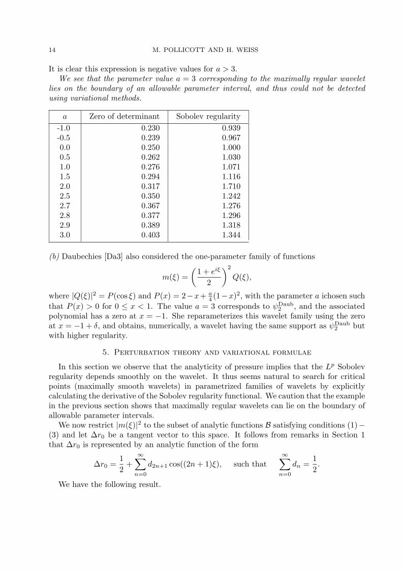
(a) Daubechies [Da1, p.242] considered the one-parameter family of filters
|m(ξ)|2 = cos2(N−1)(ξ/2)(PN−1(sin2(ξ/2)) + a cos2N (ξ/2)) cos(ξ),
where a ∈ R. For definiteness, we discuss the case N = 3. For different values of theparameter a we calculate the first zero of the determinant, and thus the Sobolev regularityof the associated wavelet using Theorem 2.2. The following table shows that this zero ismonotone increasing as a increases to 3. The zero of the determinant is 0.40344 . . . whena = 3, which corresponds to L2 Sobolev regularity 1.34443 . . . . It is not necessary to studythe case a > 3 since the expansion for |m|2 is no longer positive. To see this, we canexpand in terms of ξ − π as
|m(ξ)|2 = cos4(ξ/2)(P2(sin2(ξ/2)) + a cos4(ξ/2)) cos(ξ)
= cos4(ξ/2− π/2)(1 + 2 sin2(ξ/2− π/2) + a sin6(ξ/2− π/2) cos(ξ − π))
= sin4(ξ/2)(1 + 2 cos2(ξ/2)− a cos6(ξ/2) cos(ξ))
= 1 + 2(1− (ξ/2)2 + . . . )2 − a(1− (ξ/2)2 + . . . )6(1− ξ2 + . . . )
= (3− a)− (1 + 5a/2)ξ2 + . . . .
14 M. POLLICOTT AND H. WEISS
It is clear this expression is negative values for a > 3.We see that the parameter value a = 3 corresponding to the maximally regular wavelet
lies on the boundary of an allowable parameter interval, and thus could not be detectedusing variational methods.
a Zero of determinant Sobolev regularity-1.0 0.230 0.939-0.5 0.239 0.9670.0 0.250 1.0000.5 0.262 1.0301.0 0.276 1.0711.5 0.294 1.1162.0 0.317 1.7102.5 0.350 1.2422.7 0.367 1.2762.8 0.377 1.2962.9 0.389 1.3183.0 0.403 1.344
(b) Daubechies [Da3] also considered the one-parameter family of functions
m(ξ) =(
1 + eiξ
2
)2
Q(ξ),
where |Q(ξ)|2 = P (cos ξ) and P (x) = 2−x+ a4 (1−x)2, with the parameter a ichosen such
that P (x) > 0 for 0 ≤ x < 1. The value a = 3 corresponds to ψDaub2 , and the associated
polynomial has a zero at x = −1. She reparameterizes this wavelet family using the zeroat x = −1 + δ, and obtains, numerically, a wavelet having the same support as ψDaub
2 butwith higher regularity.
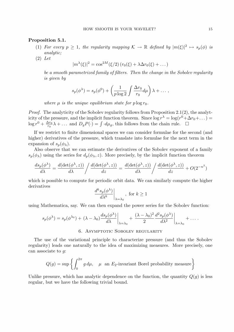
5. Perturbation theory and variational formulae
In this section we observe that the analyticity of pressure implies that the Lp Sobolevregularity depends smoothly on the wavelet. It thus seems natural to search for criticalpoints (maximally smooth wavelets) in parametrized families of wavelets by explicitlycalculating the derivative of the Sobolev regularity functional. We caution that the examplein the previous section shows that maximally regular wavelets can lie on the boundary ofallowable parameter intervals.
We now restrict |m(ξ)|2 to the subset of analytic functions B satisfying conditions (1)−(3) and let ∆r0 be a tangent vector to this space. It follows from remarks in Section 1that ∆r0 is represented by an analytic function of the form
∆r0 =12
+∞∑
n=0
d2n+1 cos((2n+ 1)ξ), such that∞∑
n=0
dn =12.
We have the following result.
HOW SMOOTH IS YOUR WAVELET? 15
Proposition 5.1.(1) For every p ≥ 1, the regularity mapping K → R defined by |m(ξ)|2 7→ sp(φ) is
analytic;(2) Let
|mλ(ξ)|2 = cos2M (ξ/2) (r0(ξ) + λ∆r0(ξ) + . . . )
be a smooth parametrized family of filters. Then the change in the Sobolev regularityis given by
sp(φλ) = sp(φ0) +(
1p log 2
∫∆r0r0
dµ
)λ+ . . . ,
where µ is the unique equilibrium state for p log r0.
Proof. The analyticity of the Sobolev regularity follows from Proposition 2.1(2), the analyt-icity of the pressure, and the implicit function theorem. Since log rλ = log(r0+∆r0+. . . ) =log r0 + ∆r0
r0λ+ . . . and DgP (·) =
∫·dµg, this follows from the chain rule. �
If we restrict to finite dimensional spaces we can consider formulae for the second (andhigher) derivatives of the pressure, which translate into formulae for the next term in theexpansion of sp(φλ).
Also observe that we can estimate the derivatives of the Sobolev exponent of a familysp(φλ) using the series for dp(φλ, z). More precisely, by the implicit function theorem
dsp(φλ)dλ
=d(det(φλ, z))
dλ
/d(det(φλ, z))
dz=d(det(φλ, z))
dλ
/d(det(φλ, z))
dz+O(2−n2
)
which is possible to compute for periodic orbit data. We can similarly compute the higherderivatives
dksp(φλ)dλk
∣∣∣∣λ=λ0
, for k ≥ 1
using Mathematica, say. We can then expand the power series for the Sobolev function:
sp(φλ) = sp(φλ0) + (λ− λ0)dsp(φλ)dλ
∣∣∣∣λ=λ0
+(λ− λ0)2
2d2sp(φλ)dλ2
∣∣∣∣λ=λ0
+ . . . .
6. Asymptotic Sobolev regularity
The use of the variational principle to characterize pressure (and thus the Sobolevregularity) leads one naturally to the idea of maximizing measures. More precisely, onecan associate to g:
Q(g) = sup{∫ 2π
0
g dµ, µ an E2-invariant Borel probability measure}
Unlike pressure, which has analytic dependence on the function, the quantity Q(g) is lessregular, but we have the following trivial bound.
16 M. POLLICOTT AND H. WEISS
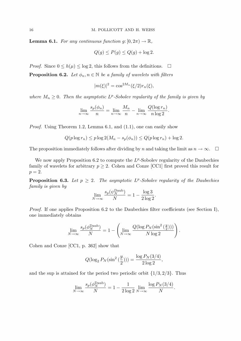
Lemma 6.1. For any continuous function g: [0, 2π) → R,
Q(g) ≤ P (g) ≤ Q(g) + log 2.
Proof. Since 0 ≤ h(µ) ≤ log 2, this follows from the definitions. �
Proposition 6.2. Let φn, n ∈ N be a family of wavelets with filters
|m(ξ)|2 = cos2Mn(ξ/2)rn(ξ),
where Mn ≥ 0. Then the asymptotic Lp-Sobolev regularity of the family is given by
limn→∞
sp(φn)n
= limn→∞
Mn
n− lim
n→∞
Q(log rn)n log 2
.
Proof. Using Theorem 1.2, Lemma 6.1, and (1.1), one can easily show
Q(p log rn) ≤ p log 2(Mn − sp(φn)) ≤ Q(p log rn) + log 2.
The proposition immediately follows after dividing by n and taking the limit as n→∞. �
We now apply Proposition 6.2 to compute the Lp-Sobolev regularity of the Daubechiesfamily of wavelets for arbitrary p ≥ 2. Cohen and Conze [CC1] first proved this result forp = 2.
Proposition 6.3. Let p ≥ 2. The asymptotic Lp-Sobolev regularity of the Daubechiesfamily is given by
limN→∞
sp(ψDaubN )N
= 1− log 32 log 2
.
Proof. If one applies Proposition 6.2 to the Daubechies filter coefficients (see Section I),one immediately obtains
limN→∞
sp(φDaubN )N
= 1−
(lim
N→∞
Q(logPN (sin2 (y2 )))
N log 2
).
Cohen and Conze [CC1, p. 362] show that
Q(log2 PN (sin2 (y
2))) =
logPN (3/4)2 log 2
,
and the sup is attained for the period two periodic orbit {1/3, 2/3}. Thus
limN→∞
sp(φDaubN )N
= 1− 12 log 2
limN→∞
logPN (3/4)N
.
HOW SMOOTH IS YOUR WAVELET? 17
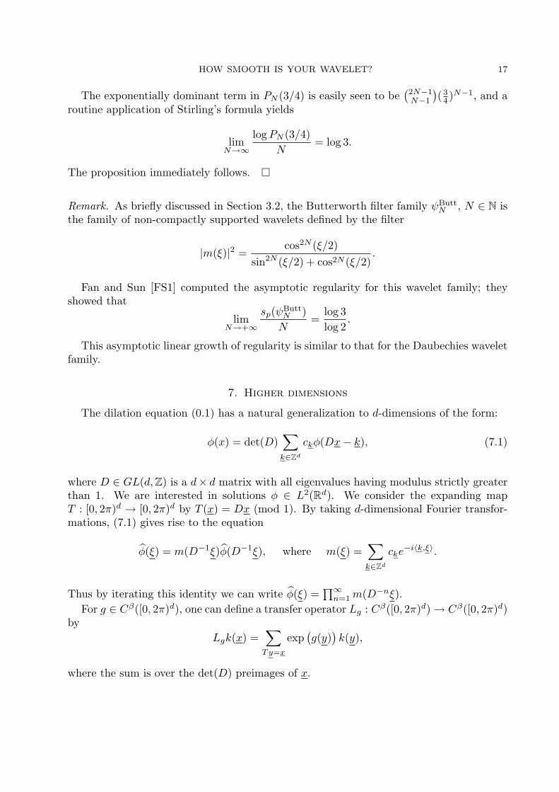
The exponentially dominant term in PN (3/4) is easily seen to be(2N−1N−1
)( 34 )N−1, and a
routine application of Stirling’s formula yields
limN→∞
logPN (3/4)N
= log 3.
The proposition immediately follows. �
Remark. As briefly discussed in Section 3.2, the Butterworth filter family ψButtN , N ∈ N is
the family of non-compactly supported wavelets defined by the filter
|m(ξ)|2 =cos2N (ξ/2)
sin2N (ξ/2) + cos2N (ξ/2).
Fan and Sun [FS1] computed the asymptotic regularity for this wavelet family; theyshowed that
limN→+∞
sp(ψButtN )N
=log 3log 2
.
This asymptotic linear growth of regularity is similar to that for the Daubechies waveletfamily.
7. Higher dimensions
The dilation equation (0.1) has a natural generalization to d-dimensions of the form:
φ(x) = det(D)∑k∈Zd
ckφ(Dx− k), (7.1)
where D ∈ GL(d,Z) is a d× d matrix with all eigenvalues having modulus strictly greaterthan 1. We are interested in solutions φ ∈ L2(Rd). We consider the expanding mapT : [0, 2π)d → [0, 2π)d by T (x) = Dx (mod 1). By taking d-dimensional Fourier transfor-mations, (7.1) gives rise to the equation
φ(ξ) = m(D−1ξ)φ(D−1ξ), where m(ξ) =∑k∈Zd
cke−i〈k,ξ〉.
Thus by iterating this identity we can write φ(ξ) =∏∞
n=1m(D−nξ).For g ∈ Cβ([0, 2π)d), one can define a transfer operator Lg : Cβ([0, 2π)d) → Cβ([0, 2π)d)
byLgk(x) =
∑Ty=x
exp(g(y)
)k(y),
where the sum is over the det(D) preimages of x.
18 M. POLLICOTT AND H. WEISS
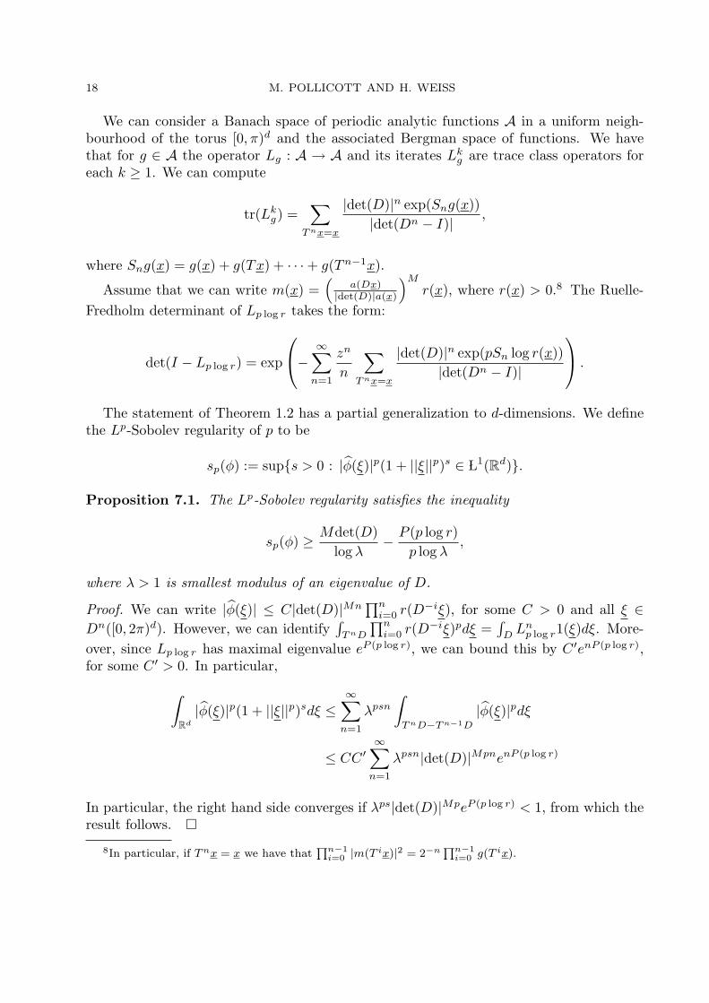
We can consider a Banach space of periodic analytic functions A in a uniform neigh-bourhood of the torus [0, π)d and the associated Bergman space of functions. We havethat for g ∈ A the operator Lg : A → A and its iterates Lk
g are trace class operators foreach k ≥ 1. We can compute
tr(Lkg) =
∑T nx=x
|det(D)|n exp(Sng(x))|det(Dn − I)|
,
where Sng(x) = g(x) + g(Tx) + · · ·+ g(Tn−1x).
Assume that we can write m(x) =(
a(Dx)|det(D)|a(x)
)M
r(x), where r(x) > 0.8 The Ruelle-Fredholm determinant of Lp log r takes the form:
det(I − Lp log r) = exp
− ∞∑n=1
zn
n
∑T nx=x
|det(D)|n exp(pSn log r(x))|det(Dn − I)|
.
The statement of Theorem 1.2 has a partial generalization to d-dimensions. We definethe Lp-Sobolev regularity of p to be
sp(φ) := sup{s > 0 : |φ(ξ)|p(1 + ||ξ||p)s ∈ L1(Rd)}.
Proposition 7.1. The Lp-Sobolev regularity satisfies the inequality
sp(φ) ≥ Mdet(D)log λ
− P (p log r)p log λ
,
where λ > 1 is smallest modulus of an eigenvalue of D.
Proof. We can write |φ(ξ)| ≤ C|det(D)|Mn∏n
i=0 r(D−iξ), for some C > 0 and all ξ ∈
Dn([0, 2π)d). However, we can identify∫
T nD
∏ni=0 r(D
−iξ)pdξ =∫
DLn
p log r1(ξ)dξ. More-over, since Lp log r has maximal eigenvalue eP (p log r), we can bound this by C ′enP (p log r),for some C ′ > 0. In particular,∫
Rd
|φ(ξ)|p(1 + ||ξ||p)sdξ ≤∞∑
n=1
λpsn
∫T nD−T n−1D
|φ(ξ)|pdξ
≤ CC ′∞∑
n=1
λpsn|det(D)|MpnenP (p log r)
In particular, the right hand side converges if λps|det(D)|MpeP (p log r) < 1, from which theresult follows. �
8In particular, if T nx = x we have thatQn−1
i=0 |m(T ix)|2 = 2−nQn−1
i=0 g(T ix).
HOW SMOOTH IS YOUR WAVELET? 19
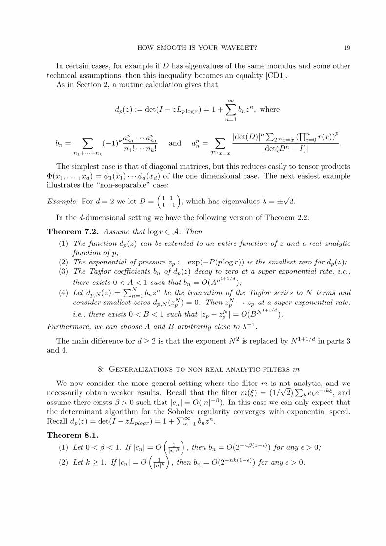
In certain cases, for example if D has eigenvalues of the same modulus and some othertechnical assumptions, then this inequality becomes an equality [CD1].
As in Section 2, a routine calculation gives that
dp(z) := det(I − zLp log r) = 1 +∞∑
n=1
bnzn, where
bn =∑
n1+···+nk
(−1)k apn1· · · ap
n1
n1! · · ·nk!and ap
n =∑
T nx=x
|det(D)|n∑
T nx=x (∏n
i=0 r(x))p
|det(Dn − I)|.
The simplest case is that of diagonal matrices, but this reduces easily to tensor productsΦ(x1, . . . , xd) = φ1(x1) · · ·φd(xd) of the one dimensional case. The next easiest exampleillustrates the “non-separable” case:
Example. For d = 2 we let D =(
1 1
1 −1
), which has eigenvalues λ = ±
√2.
In the d-dimensional setting we have the following version of Theorem 2.2:
Theorem 7.2. Assume that log r ∈ A. Then(1) The function dp(z) can be extended to an entire function of z and a real analytic
function of p;(2) The exponential of pressure zp := exp(−P (p log r)) is the smallest zero for dp(z);(3) The Taylor coefficients bn of dp(z) decay to zero at a super-exponential rate, i.e.,
there exists 0 < A < 1 such that bn = O(An1+1/d
);(4) Let dp,N (z) =
∑Nn=1 bnz
n be the truncation of the Taylor series to N terms andconsider smallest zeros dp,N (zN
p ) = 0. Then zNp → zp at a super-exponential rate,
i.e., there exists 0 < B < 1 such that |zp − zNp | = O(BN1+1/d
).
Furthermore, we can choose A and B arbitrarily close to λ−1.
The main difference for d ≥ 2 is that the exponent N2 is replaced by N1+1/d in parts 3and 4.
8: Generalizations to non real analytic filters m
We now consider the more general setting where the filter m is not analytic, and wenecessarily obtain weaker results. Recall that the filter m(ξ) = (1/
√2)∑
k cke−ikξ, and
assume there exists β > 0 such that |cn| = O(|n|−β). In this case we can only expect thatthe determinant algorithm for the Sobolev regularity converges with exponential speed.Recall dp(z) = det(I − zLplogr) = 1 +
∑∞n=1 bnz
n.
Theorem 8.1.
(1) Let 0 < β < 1. If |cn| = O(
1|n|β
), then bn = O(2−nβ(1−ε)) for any ε > 0;
(2) Let k ≥ 1. If |cn| = O(
1|n|k
), then bn = O(2−nk(1−ε)) for any ε > 0.
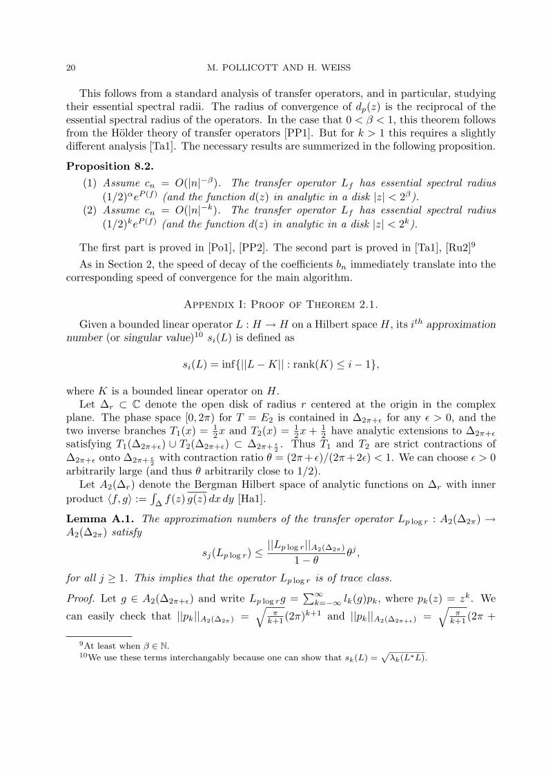
20 M. POLLICOTT AND H. WEISS
This follows from a standard analysis of transfer operators, and in particular, studyingtheir essential spectral radii. The radius of convergence of dp(z) is the reciprocal of theessential spectral radius of the operators. In the case that 0 < β < 1, this theorem followsfrom the Holder theory of transfer operators [PP1]. But for k > 1 this requires a slightlydifferent analysis [Ta1]. The necessary results are summerized in the following proposition.
Proposition 8.2.
(1) Assume cn = O(|n|−β). The transfer operator Lf has essential spectral radius(1/2)αeP (f) (and the function d(z) in analytic in a disk |z| < 2β).
(2) Assume cn = O(|n|−k). The transfer operator Lf has essential spectral radius(1/2)keP (f) (and the function d(z) in analytic in a disk |z| < 2k).
The first part is proved in [Po1], [PP2]. The second part is proved in [Ta1], [Ru2]9
As in Section 2, the speed of decay of the coefficients bn immediately translate into thecorresponding speed of convergence for the main algorithm.
Appendix I: Proof of Theorem 2.1.
Given a bounded linear operator L : H → H on a Hilbert space H, its ith approximationnumber (or singular value)10 si(L) is defined as
si(L) = inf{||L−K|| : rank(K) ≤ i− 1},
where K is a bounded linear operator on H.Let ∆r ⊂ C denote the open disk of radius r centered at the origin in the complex
plane. The phase space [0, 2π) for T = E2 is contained in ∆2π+ε for any ε > 0, and thetwo inverse branches T1(x) = 1
2x and T2(x) = 12x + 1
2 have analytic extensions to ∆2π+ε
satisfying T1(∆2π+ε) ∪ T2(∆2π+ε) ⊂ ∆2π+ ε2. Thus T1 and T2 are strict contractions of
∆2π+ε onto ∆2π+ ε2
with contraction ratio θ = (2π+ ε)/(2π+2ε) < 1. We can choose ε > 0arbitrarily large (and thus θ arbitrarily close to 1/2).
Let A2(∆r) denote the Bergman Hilbert space of analytic functions on ∆r with innerproduct 〈f, g〉 :=
∫∆f(z) g(z) dx dy [Ha1].
Lemma A.1. The approximation numbers of the transfer operator Lp log r : A2(∆2π) →A2(∆2π) satisfy
sj(Lp log r) ≤||Lp log r||A2(∆2π)
1− θθj ,
for all j ≥ 1. This implies that the operator Lp log r is of trace class.
Proof. Let g ∈ A2(∆2π+ε) and write Lp log rg =∑∞
k=−∞ lk(g)pk, where pk(z) = zk. We
can easily check that ||pk||A2(∆2π) =√
πk+1 (2π)k+1 and ||pk||A2(∆2π+ε) =
√π
k+1 (2π +
9At least when β ∈ N.10We use these terms interchangably because one can show that sk(L) =
pλk(L∗L).
HOW SMOOTH IS YOUR WAVELET? 21
ε)k+1. The functions {pk}k∈Z form a complete orthogonal family for A2(∆2π+ε), and so〈Lp log rg, pk〉A2(∆2π+ε) = lk(g)||pk||2A2(∆2π+ε)
. The Cauchy-Schwarz inequality implies that
|lk(g)| ≤ ||Lp log rg||A2(∆2π+ε) ||pk||−1A2(∆2π+ε)
.
We define the rank-j projection operator by L(j)p log r(g) =
∑j−1k=0 lk(g)pk. For any g ∈
A2(∆θ) we can estimate
||(Lp log r − L
(j)p log r
)(g)||A2(∆2π) ≤ ||Lp log rg||A2(∆2π)
∞∑k=j
θk+1.
It follows that
||Lp log r − L(j)p log r||A2(∆2π) ≤
||Lp log r||A2(∆2π)
1− θθj+1,
and so
sj+1(Lp log r) ≤||Lp log r||A2(∆2π)
1− θθj+1,
and the result follows. �
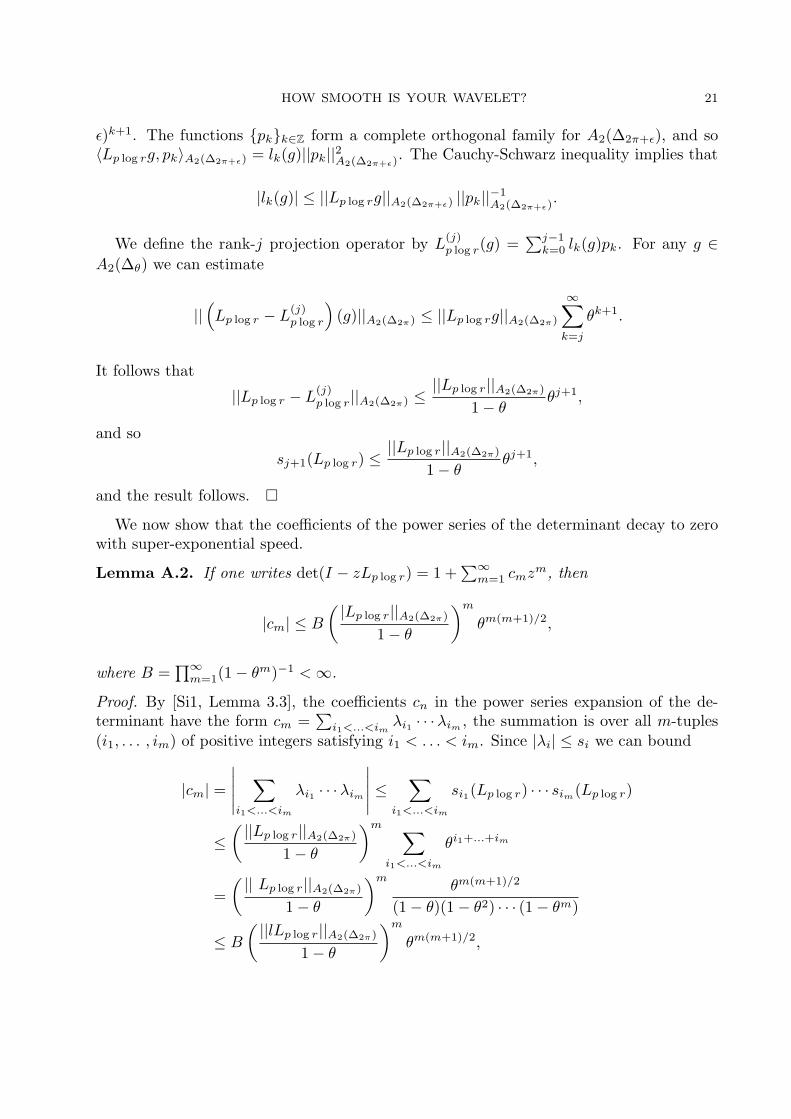
We now show that the coefficients of the power series of the determinant decay to zerowith super-exponential speed.
Lemma A.2. If one writes det(I − zLp log r) = 1 +∑∞
m=1 cmzm, then
|cm| ≤ B
( |Lp log r||A2(∆2π)
1− θ
)m
θm(m+1)/2,
where B =∏∞
m=1(1− θm)−1 <∞.
Proof. By [Si1, Lemma 3.3], the coefficients cn in the power series expansion of the de-terminant have the form cm =
∑i1<...<im
λi1 · · ·λim , the summation is over all m-tuples(i1, . . . , im) of positive integers satisfying i1 < . . . < im. Since |λi| ≤ si we can bound
|cm| =
∣∣∣∣∣ ∑i1<...<im
λi1 · · ·λim
∣∣∣∣∣ ≤ ∑i1<...<im
si1(Lp log r) · · · sim(Lp log r)
≤( ||Lp log r||A2(∆2π)
1− θ
)m ∑i1<...<im
θi1+...+im
=( || Lp log r||A2(∆2π)
1− θ
)mθm(m+1)/2
(1− θ)(1− θ2) · · · (1− θm)
≤ B
( ||lLp log r||A2(∆2π)
1− θ
)m
θm(m+1)/2,
22 M. POLLICOTT AND H. WEISS
for some B > 0. �
We finish by showing that Theorem 2.1 follows from Lemma 2.2. The coefficients ofdet(I − zLs) = 1 +
∑∞n=1 bnz
n are given by Cauchy’s Theorem:
|bn| ≤1rn
sup|z|=r
|det(I − zLs)|, for any r > 0.
Using Weyl’s inequality we can deduce that if |z| = r then
|det(I − zLs)| ≤∞∏
j=1
(1 + |z|λj) ≤∞∏
j=1
(1 + |z|sj)
≤
(1 +B
∞∑m=1
(rα)mθm(m+1)
2
)
where α = ||Ls||A2(∆2π). If we choose r = r(n) appropriately then we can get the boundsgiven in the theorem.
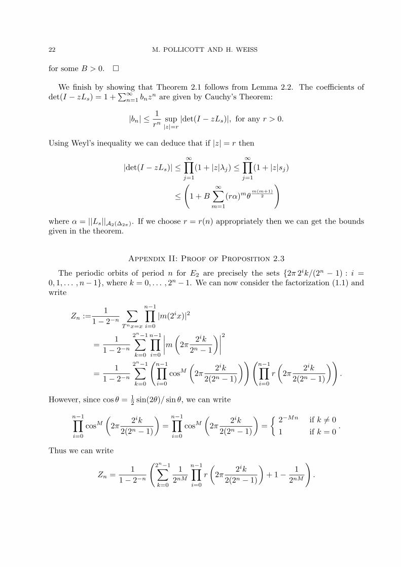
Appendix II: Proof of Proposition 2.3
The periodic orbits of period n for E2 are precisely the sets {2π 2ik/(2n − 1) : i =0, 1, . . . , n− 1}, where k = 0, . . . , 2n − 1. We can now consider the factorization (1.1) andwrite
Zn :=1
1− 2−n
∑T nx=x
n−1∏i=0
|m(2ix)|2
=1
1− 2−n
2n−1∑k=0
n−1∏i=0
∣∣∣∣m(2π2ik
2n − 1
)∣∣∣∣2
=1
1− 2−n
2n−1∑k=0
(n−1∏i=0
cosM
(2π
2ik
2(2n − 1)
))(n−1∏i=0
r
(2π
2ik
2(2n − 1)
)).
However, since cos θ = 12 sin(2θ)/ sin θ, we can write
n−1∏i=0
cosM
(2π
2ik
2(2n − 1)
)=
n−1∏i=0
cosM
(2π
2ik
2(2n − 1)
)={
2−Mn if k 6= 01 if k = 0
.
Thus we can write
Zn =1
1− 2−n
(2n−1∑k=0
12nM
n−1∏i=0
r
(2π
2ik
2(2n − 1)
)+ 1− 1
2nM
).
HOW SMOOTH IS YOUR WAVELET? 23
Since (1− 2−nM )/(1− 2−n) =∑M−1
j=0 2−jn, we can write
det(1− zLp log |m|2) = exp
∞∑n=0
M−1∑j=0
(z2−j)n
det(
1− z
2MLp log r
)
=M−1∏j=0
(1− z2−j
)det(
1− z
2MLp log r
).
�
References
[CC1] A. Cohen and J.-P. Conze, Regularite des bases d’ondelettes et mesures ergodiques., Rev. Mat.Iberoamericana 8 (1992), 351–365.
[CD1] A. Cohen and I. Daubechies, A new technique to estimate the regularity of refinable functions,
Rev. Mat. Iberoamericana 12 (1996), 527–591.
[Da1] I. Daubechies, Ten lectures on wavelets, CBMS-NSF Regional Conference Series in Applied
Mathematics, vol. 61, Society for Industrial and Applied Mathematics (SIAM), 1992.
[Da2] I. Daubechies, Using Fredholm determinants to estimate the smoothness of refinable functions,Approximation theory VIII, Vol. 2 (College Station, TX, 1995), Ser. Approx. Decompos. 6
(1995), World Sci. Publishing, 89–112.
[Da3] I. Daubechies, Orthonormal Bases of Compactly Supported Wavelets II, SIAM J. Math. Anal.
24 (1993), 499–519.
[Ei1] T. Eirola, Sobolev characterization of solutions of dilation equations., SIAM J. Math. Anal.23 (1992), 1015–103.
[FS1] A. Fan and Q. Sun, Regularity of Butterworth Refinable Functions, preprint.
[GGK1] I. Gohberg, S. Goldberg and M. A. Kaashoek, Classes of linear operators, vol 1, 1990.
[Ha1] P. Halmos, Introduction to Hilbert space and the theory of spectral multiplicity, reprint of the
second (1957) edition, AMS Chelsea Publishing, Providence, RI,, 1998.
[He1] L. Herve, Comportement asymptotique dans l’algorithme de transformee en ondelettes, Rev.
Mat. Iberoamericana 11 (1985), 431–451.
[He2] L. Herve, Construction et regularite des fonctions d’chelle, SIAM J. Math. Anal. 26 (1995),1361–1385.
[JP1] O. Jenkinson and M. Pollicott, Computing invariant densities and metric entropy, Comm.
Math. Phys. 211 (2000), 687–703.
[JP2] O. Jenkinson and M. Pollicott, Orthonormal expansions of invariant densities for expanding
maps, Advances in Mathematics, 192 (2005), 1-34.
[Oj1] H. Ojanen, Orthonormal compactly supported wavelets with optimal sobolev regularity, Appliedand Computational Harmonic Analysis 10 (2001), 93-98.
[OS1] A. Oppenheim and R. Shaffer, Digital Signal Processing, Pearson Higher Education, 1986.
[PP1] W. Parry and M. Pollicott, Zeta Functions and the Periodic Orbit Structures of Hyperbolic
Dynamics, Asterisque 187–188 (1990).
[Po1] M. Pollicott, Meromorphic extensions for generalized zeta functions, Invent. Math 85 (1986),
147–164.
[Ru1] D. Ruelle, Thermodynamic Formalism, Addison-Wesley, 1978.
[Ru2] D. Ruelle, An extension of the theory of Fredholm determinants, Inst. Hautes tudes Sci. Publ.Math. 72 (1990), 175–193.
[Ru2] D. Ruelle, An extension of the theory of Fredholm determinants, Inst. Hautes tudes Sci. Publ.
Math. 72 (1990), 175–193.
24 M. POLLICOTT AND H. WEISS
[Si1] B. Simon, Trace ideals and their applications, LMS Lecture Note Series, vol. 35, CambridgeUniversity Press, 1979.
[Ta1] F. Tangerman, Meromorphic continuation of Ruelle zeta functions, Ph.D. Thesis, Boston
University (1988).[Vi1] L. Villemoes, Energy moments in time and frequency for two-scale difference equation solu-
tions and wavelets, SIAM J. Math. Anal. 23 (1992), 1519–1543.
[W] Matlab, Wavelet Toolbox Documentation, www.mathworks.com/access/helpdesk/help/tool-box/wavelet/wavelet.html?BB=1.