1

Cav03-OS-6-001 Fifth International Symposium on Cavitation (cav2003)

Osaka, Japan, November 1-4, 2003

HUB SHAPE EFFECTS UNDER CAVITATION ON THE INDUCERS PERFORMANCE

Farid Bakir, LEMFI-ENSAM farid.bakir@paris.ensam.fr

Imen Mejri, LEMFI-ENSAM imen.mejri@paris.ensam.fr

Smaine Kouidri, LEMFI-ENSAM smaine.kouidri@paris.ensam.fr

Robert Rey, LEMFI-ENSAM Robert.rey@paris.ensam.fr

ABSTRACT Experimental and numerical investigations were performed

to study the hub shape effects on the inducers performance. Three inducers are compared. They have the same tip blade angle at inlet and have various hub shapes: two inducers have a cylindrical hub and the third has a conical hub. A bibliographic review of the cavitating regime is firstly presented. Then, the main results are presented for the three inducers:

• Overall performance: head coefficient and critical cavitation number (5% and 15% of drop) versus the flow rate.

• Vibration behavior versus the flow rate and the suction pressure.

• The computational 3D flow in non-cavitation regime, carried out CFX BladeGEN+ code. This enabled us to explain the unstable and cavitating operation for off-design conditions.

Lastly, the numerical computation in cavitating flow carried out using the CFX-TASCFlow 2.12 is presented. The validation of the model was done on BH inducer. The comparisons between experimental and simulated results on the overall performance, head drop and cavitation figures are discussed.

INTRODUCTION

The inducer is generally located upstream of a centrifugal or mixed flow impeller in order to improve its behavior in a cavitation regime. The two rotors are assembled on the same driving shaft and are powered at the same rotational speed. The inducer is engineered to resist to the cavitation. It generates an increase of the pressure and therefore allows the principal impeller to operate with better inlet conditions. Aerospace research has contributed the most significant progress to the knowledge of cavitating flows and the improvement of inducer’s performance [1].

The association of the inducer and impeller is common in modern industrial applications: nuclear power, petroleum, food industry, and chemistry.... with, the best performance for fuel pumping and cryogenic rocket fuel.

This device enables higher rotational speeds which results in more compact pumps and generally more economical. The cavitation causes operational instability and vibration, which compromise their performance, mainly in the off-design condition.

The blade cavitation and the tip clearance cavitation, which can appear at any flow rate, can also have a backflow mode superimposed that makes the cavitation very unstable. The effects are amplified when the flow rate decreases. The intensity of this phenomenon depends on the general blade design and on the upstream environment [2-3].

Although the use of inducers is frequent today, several aspects of their operation and their behavior still remain difficult to model. In order to appreciate some phenomena, which affect the reliability of these devices, their maximum performance and their operational limits, we still rely on experimentation.

NOMENCLATURE Cm meridional velocity [m/s] DT tip diameter [m] g gravity acceleration [m/s] H head [m] i=β1T-β1 incidence angle [°] N rotational speed [rpm] NPSH Net Positive Suction Head [m] NPSH5% NPSH corresponding to 5% of head drop [m] pv liquid vapor pressure [Pa] Q flow rate [m3/s] RT tip radius [m] RH hub radius [m]

75,0%5 ).(.9326.52

NPSHgQ

Sω

= suction specific speed [-]

T=RH/RT hub to tip ratio [-] U1T peripheral velocity [m/s] W relative velocity [m/s] β1T tip blade angle at inlet [°] ηMAX best efficiency [%]

2

11

1 βφ tgU

C

T

m == flow coefficient [-]

φN flow coefficient at design point [-] φS flow coefficient at Smax [-]

RgH

T22ω

ψ = pressure coefficient [-]

γ stagger angle [°] ρ liquid density [kg/m3]

2221

T

Nc

R

gNPSH

ωσ = cavitation number [-]

ω angular velocity [rad/s]

1 FLOW MODELING IN A REGIME OF CAVITATION The appearance of the cavitating structures, their geometry

and more generally their static and dynamic properties, depend on several parameters which include above all: the blade profile, camber, incidence, stacking, and leading edge shape, as well as roughness of the walls, the upstream turbulence, the existence of gas micro-bubbles in the flow, the fluid viscosity, etc…

When operating close to the design flow rate, the appearance of cavitation (first bubble) is computable under satisfactory conditions.

The blade cavitation has been the subject of many models, essentially 2D using potential flow, which are capable of describing the lengthening of the vapor pocket along the blades. The shape of the attached cavity is obtained after an iterative process and constitutes the limit of the isobar p = pv in the pressure field between blades of the rotor grid (model with interface). It should be noted that an empirical model of the vapor pocket wake is used [4-5].

The cavitating pockets can come from several natures; some remain attached to the blades with more or less oscillating lengths and frequencies of release, which can vary from a blade to another. They can also be rotating with different rotation frequencies compared to the ones of the impeller.

According to the present authors' experience, the pressure drop starts when the cavitating pocket reaches the throat formed by two successive blades where it is quickly dragged to the trailing edge. While retaining this particular criterion for the calculated pocket, we obtain a good approach of the critical NPSH in a range of incidence close to the design point.

Several authors [6-9] studied in a global and generalized way the cavitating flow.

In a general way, the majority of the suggested cavitation models are based on assumptions, which are similar. They are either two-dimensional or three-dimensional and steady. Recently, some of the models of cavitation were introduced into software’s based on the three-dimensional unsteady equations of Navier-Stokes. It allows the extension of these codes to calculate the cavitation in turbomachines.

Among the authors who combined the cavitation models with the CFD tools one can quote:

• for the 3D analysis of cavitating flows: Frobenius et al. [10] which used the code CNS3D based on the developed model by Sauer and Schnerr [11] and

Coutier-Delgosha et al. [12] which relied on to the code: FINE/TURBO of NUMECA.

• for centrifugal pumps: Athavale et al. [13], Singhal et al. [14], Reboud and Delannoy [15].

• concerning the inducers, a few authors published on this subject: Horiguchi et al. [16].

A way to classify the models about cavitating flow is to distinguish them into two different classes: multi-phase models and single fluid models.

For these two categories, the analysis of the cavitating flow is made through the resolution of the traditional mass and momentum equations and sometimes energy. This method is used for two areas: area with the full liquid flow and one another for the cavitation one. We will distinguish then:

- models whose interface has already been described. - multi-phase models: models with 2 phases (such as the

VOF) and models with 3 phases based on the traditional conservation equations for each phase (liquid phase, vapor phase and possibly non-condensable gas phase), correlations and the empirical relations for the exchange terms of heat/mass/momentum between the phases supposed in non-equilibrium. For the latter, the state equations are frequently added (such as the assumption of ideal gas) with the Tait equation, the assumption of low compressibility of the liquid, the barotropic relations of the range p = f(ρ), the logarithmic correlation of Schmidt, etc ... Thus, the problem lies in the determination of the exchange terms for heat/mass/momentum.

- single fluid models: based on the conservation equations for only one phase composed of a liquid/vapor mixture. This phase is provided with single speed only (average speed) and one density for the mixture. Added to these equations we used the state equations with the assumption of local thermodynamic equilibrium between the liquid and vapor phases. Nevertheless in the reality and during an expansion process, the transfers of heat and mass between the phases are not in the equilibrium conditions. Indeed, the expansion is a fast process and vaporization requires a great quantity of energy (to be taken from the surrounding fluid). Moreover, the assumption of thermal equilibrium starts to be invalid for the case where the fluid acceleration is significant, because in such flows, the terms of mass and heat transfer between the phases vary much more slowly than the pressure gradients.

Numerically, we can classify the cavitation models in models whose calculations are carried out in only one channel and others which calculate simultaneously between all the blades taking into account their various interactions. 2 PRESENTATION OF THREE INDUCERS AND TEST RIG

Three inducers are compared. They have the different hub shapes: two inducers have a cylindrical hub and the third has a conical hub. These inducers are named BH inducer, SH inducer and CH inducer in order as shown in figure 1. The hub ratio is equal to, 0.475 for the BH inducer, 0.25 for the SH inducer and respectively, to 0.25 and 0.475 at blades inlet and outlet for CH inducer. The inducers have three blades with a constant thickness and the swept back leading edge. The sweep angle at the tip is 95 degrees. The tip diameter is 234 mm. The inlet

3

blade angle is 15 degrees. This angle is constant from inlet to outlet. The principal dimensions of the three test inducers are shown in table 1.

BH Inducer SH Inducer CH Inducer Figure 1 - Pictures of the three inducers.

Rotational speed 1450 rpm Blades number 3 Blade thickness 5 mm Tip blade angle 15° Tip solydity Tip diameter 234 mm Tip clearance 0.4 mm Inducer BH SH° CH°Flow coefficient 0.087 0.121 0.136 Head coefficient 0.133 0.105 0.105 Hub to tip ratio in inlet 0.47 0.22 0.22 Hub to tip ratio in outlet 0.47 0.22 0.47

Table 1 - Main constructive parameters of the inducers.

General overview of the test rig

The LEMFI-Paris axial and centrifugal pumps test rig, is composed of the following main elements (figure 2): - Two storage tanks with a capacity of 4 m3 each, connected by a 350 mm diameter pipe. They can be loaded and emptied using two electrical control valves. - A liquid ring vacuum pump is used to control the pressure at the free surface inside the storage tanks. - A 22 kW alternative motor powered by a variable frequency controller was used to drive the tested inducer. The manufacturer gives the electric efficiency of the motor. The rotational speed is measured using a magnetic tachometer (accuracy 0.1%). - A motorized control valve serves to adjust precisely the flow rate. - The inducer equipped with a transparent acrylic cover. - A centrifugal pump installed in series with the impeller in order to overcome the circuit losses. - Various measurement instruments and devices: Ultrasonic flow meter (″A500 - Sparling Meter Flow ″,

accuracy 1%), placed at the inlet of the inducer. Two piezoresistif manometers (Kistler, type 601A, accuracy

1%). They are positioned at the inlet and outlet sections and measure the average tip pressure (at about 20 mm upstream of the leading edge and 150 mm downstream of the trailing edge of the blade). The signal resulting from these sensors is amplified then treated by a Lecroy spectrum analyzer

(type 930 4A). Its connection with a computer enables us to store and to use these signals.

A temperature probe (accuracy 1%): the average temperature during the tests presented below is 18°C.

Figure 2 - Hydrodynamic test bench of the LEMFI - Paris. 3 COMPARISON OF THE INDUCERS PERFORMANCE

This section compares the performance of the three machines, namely: overall performance (head, flow rate, efficiency), the behavior with cavitation characterized by the cavitation coefficient σC and the fluctuations pressure level at the inducer outlet. Overall performance

Overall performance in non-cavitation regime (figure 3) is higher for the SH inducer, with a hydraulic efficiency which increases from 57 to 70%.

0.00 0.05 0.10 0.15 0.20φ

0.00

0.10

0.20

0.30

ψ

Overall Performance 1450 rpm

SH inducer

BH inducer

CH inducer

Figure 3 – hub shape influence on the overall performance. For the values corresponding to the best efficiency, the

following table gives the flow coefficient and the incidence angles:

Inducer ηMAX φN i/β1T

BH 0,57 0,173 0,35 SH 0,70 0,153 0,42 CH 0,68 0,173 0,35

Table 2 - Main constructive parameters of the inducers.

4

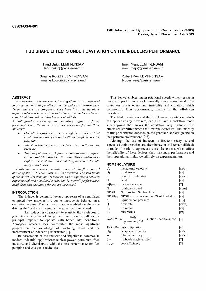
Behavior in cavitating regime The behavior in cavitating regime is characterized by the cavitation parameter σC corresponding to a head drop of 5% and 15%. The test results are given, as an example, for the SH inducer on figure 4. The rounded shape of the head drop in off-design flow rate is a characteristic of the rotating cavitation [17]. For this reason, a significant difference appears concerning the σC 5% and 15% of head drop.

Figure 4 - Pressure drop curve versus the σC.

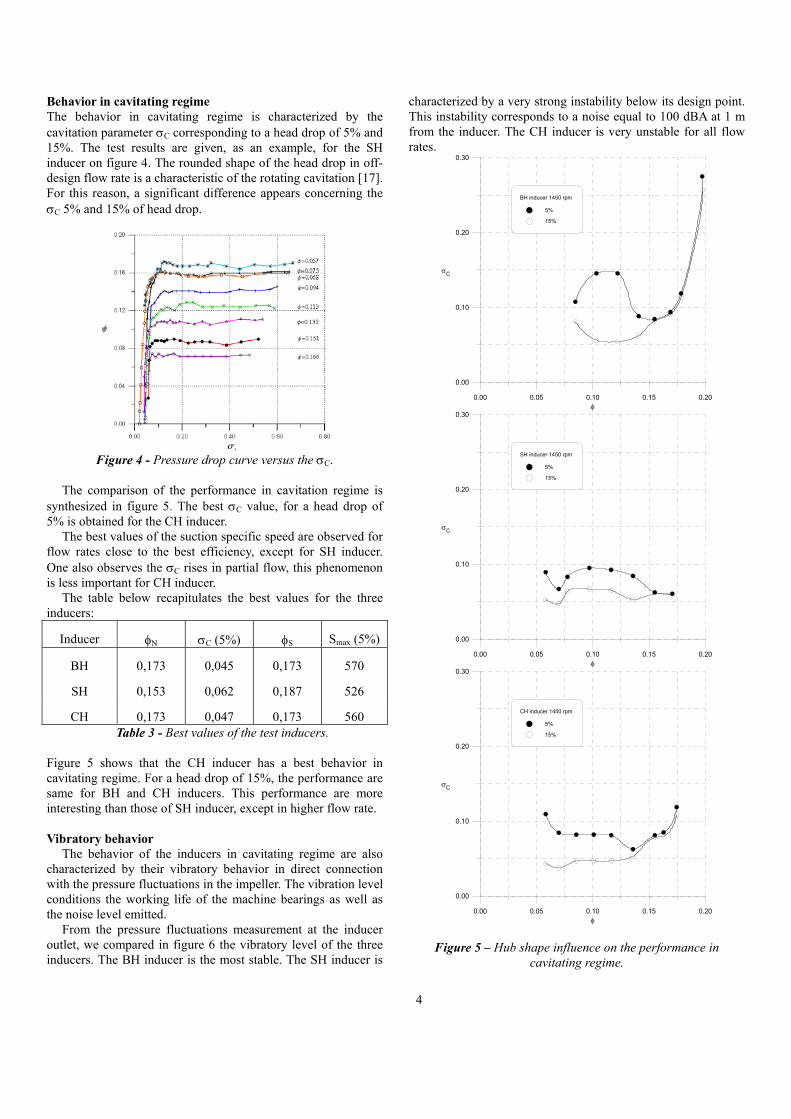
The comparison of the performance in cavitation regime is synthesized in figure 5. The best σC value, for a head drop of 5% is obtained for the CH inducer.

The best values of the suction specific speed are observed for flow rates close to the best efficiency, except for SH inducer. One also observes the σC rises in partial flow, this phenomenon is less important for CH inducer.

The table below recapitulates the best values for the three inducers:

Inducer φN σC (5%) φS Smax (5%)

BH 0,173 0,045 0,173 570

SH 0,153 0,062 0,187 526

CH 0,173 0,047 0,173 560 Table 3 - Best values of the test inducers.

Figure 5 shows that the CH inducer has a best behavior in cavitating regime. For a head drop of 15%, the performance are same for BH and CH inducers. This performance are more interesting than those of SH inducer, except in higher flow rate. Vibratory behavior

The behavior of the inducers in cavitating regime are also characterized by their vibratory behavior in direct connection with the pressure fluctuations in the impeller. The vibration level conditions the working life of the machine bearings as well as the noise level emitted.

From the pressure fluctuations measurement at the inducer outlet, we compared in figure 6 the vibratory level of the three inducers. The BH inducer is the most stable. The SH inducer is

characterized by a very strong instability below its design point. This instability corresponds to a noise equal to 100 dBA at 1 m from the inducer. The CH inducer is very unstable for all flow rates.

0.00 0.05 0.10 0.15 0.20φ

0.00

0.10

0.20

0.30

σC

BH inducer 1450 rpm

5%

15%

0.00 0.05 0.10 0.15 0.20φ

0.00

0.10

0.20

0.30

σC

SH inducer 1450 rpm

5%

15%

0.00 0.05 0.10 0.15 0.20φ

0.00

0.10

0.20

0.30

σC

CH inducer 1450 rpm

5%

15%

Figure 5 – Hub shape influence on the performance in

cavitating regime.

5

0.00 0.05 0.10 0.15 0.20Φ

0.00

0.20

0.40

0.60

σ

BH Inducer

c

ΦN

0.00 0.05 0.10 0.15 0.20Φ

0.00

0.20

0.40

0.60

σ

SH Inducer

c

ΦN

0.00 0.05 0.10 0.15 0.20Φ

0.00

0.20

0.40

0.60

σ c

ΦN

CH Inducer

Figure 6 - Pressure fluctuations levels versus σC and flow rate.

This phenomenon is related to the backflow cavitation and to

the rotating cavitation created by the tip vortex. It is located at the leading edge and propagates toward upstream. To describe these irregular phenomena’s, CFD computations have been made on the three inducers. The CFD code used is Blade GEN+, 3D Navier Stockes code with a Zero equation turbulence model and a non structured grid generator with tetrahedral elements. The computations were made under non-cavitating steady flow condition for several flow rates.

The simulation conditions are: N = 1450 rpm with the condition of mass flow rate imposed at the outlet and static pressure at the inlet. The tip clearance is not take into account here. The mesh size is approximately 45000 nodes. The figures 7, 8 and 9 show, for various flow rates, the magnitude and the

direction of meridional velocity circumferentially averaged. The blade-to-blade flow is shown at the tip radius. BH Inducer (figures 7 and 6-a).

For φN = 0,173, the inducer is very stable and the meridional flow is relatively uniform (figure 6 a). For φ = 0,14 the backflow vortex is formed (figure 7): it is the beginning of the increase of the pressure fluctuations level. At φ = 0,094 the vortex is amplified and the pressure fluctuations level remains high. SH Inducer (figure 8 and 6 b) .

For φS = 0.187 the meridional flow is well organized and a flow rate decrease is observed at the tip. For φ = 0.113 and φ = 0.094, the backflow vortex is amplified. CH Inducer (figures 9 and 6 c). For the respective flow rate coefficients of 0.100, 0.148 and φN = 0,173, the phenomena are the same as the one previously described. Here the backflow appears close to the nominal flow rate.

For the three machines, the coupling between the backflow vortex and the cavitation generates the very high vibrations level. The figure 10 shows for φ = 0.094 versus σC the appearance of the cavitation figures. The cavitation pocket are first extends forwards (σC =0.13, very unstable zone). On the same figure, 3D computation shows, for the peripheral grid, the same phenomena. The pocket has the same orientation but its extent is amplified by the presence of the tip clearance. When the σC decreases, we observe the attached pockets, which will lead the drop performance. It is a phenomenon of partial flow rate described in reference [18]. 4 CFX-TASCFLOW 2.12 VOF MODEL The cavitation model implemented in the Commercial CFD software CFX-TASCflow 2.12 is used. The validation of the model was performed, at various flow rates, on the cavitating behavior of BH inducer. After a grid dependence solution study, a 250000-structured mesh for a single blade passage was used for all the computations (figure 11). This mesh was created using the mesh generator CFX-TurboGrid. The boundary conditions used are: total pressure at the inlet and mass flow at the outlet. The connection between the periodic faces is made by periodic connections. The standard two-equation k-ε model was used for modelling the turbulence. The convergence criteria were set to 1e-4 on the maximal residual. For all the numerical simulations, the tip clearance was not taken into account. For each flow rate, the head drop curve was created as follow:

First, an incompressible solution without cavitation is computed. From this non-cavitation solution, the VOF model is turn on while the total pressure at the inlet is decreased by a constant step of 10000 Pa. Close to the drop zone, this step is reduced by a factor of 10 and more to overcome the high instability of the solution due to the strong non-linear behavior of the cavitation. Thus, the head drop curve is created gradually. We note finally that the time consuming for the creation of a whole one head drop curve is about 8h on machine having 2 CPU.

6

Figure 7 – BH inducer - Evolution of the meridional flow versus flow rate.

Figure 8 – SH inducer Evolution of the meridional flow versus flow rate.

Figure 9 – CH inducer - Evolution of the meridional flow versus flow rate.

Figure 10 – SH inducer - Head drop curves and associated

figures of cavitation in partial flow rate (φ = 0,094).

7

Figure 11 - typical Mesh used for the simulation.

Overall performance For non-cavitation regime, figure 12 shows the evolution of the experimental and predicted values of the pressure coefficient versus the flow rate. As shown, a good agreement between the two results is obtained at nominal and high flow rates. At low flow rates, the difference between the two results is due to the tip clearance effects. For several flow rates, figure 13 shows the predicted values of the pressure coefficient versus the cavitation number σ. Figure 14 shows the experimental and predicted values of the critical cavitation number σc versus the flow rate. This critical cavitation number corresponds to 5% of the head drop.

At low flow rates (qv/qn=0.55 to qv/qn=0.79), the drop curve occurs smoothly and slightly before the experimental one. Close to design flow rates (qv/qn=0.91 to qv/qn=1.09), the drop curve occurs suddenly and simultaneously with the experimental one. The agreement between the two results is very satisfactory. At high flow rates (qv/qn=1.15 to qv/qn=1.27), the drop curve occurs suddenly and slightly after the experimental one. For the very high flow rate (qv/qn=1.27), the blockage phenomenon has occurred experimentally and not yet numerically. The VOF model under predicted the blockage phenomenon and could be attribute to the turbulence modelling and also to the presence of empirical coefficient of vaporisation-condensation in model.

Figure 12 – Head coefficient versus flow rate.

0.00 0.20 0.40 0.60 0.80σ

0.00

0.10

0.20

0.30

ψ

Q/Qn=1.27

Q/Qn=1.15

Q/Qn=1.09

Q/Qn=1.03

Q/Qn=0.91

Q/Qn=0.79

Q/Qn=0.67

Q/Qn=0.55

BH INDUCER 1450 rpm

Figure 13 - Predicted performance.

0.00 0.20 0.40 0.60 0.80 1.00 1.20 1.40 1.60qv/qn

0.00

0.05

0.10

0.15

0.20

0.25

0.30

0.35

0.40

0.45

0.50

σ

Experimental

CFX-TASCflow

C

N = 1450 rpm

Figure 14 -critical cavitation number vs. flow rate.

Cavitation visualization For the computed results, the vapor rate is specified. The size of the predicted cavitation pocket corresponds to 10% of vapor in the mixture. This is leads to an incertainty of the experimental vapor percentage in the mixture and 10% was a realistic value to be used. The hub is paint in green, the blade in red and the cavitation zone in blue. The predicted cavitation behaviors are typical and in general in conformity with those visualized experimentally. Figure 15 presents the most representative images. One can thus identify:

• In partial flow rates, backflow vortex cavitation returning upstream of the inducer (figure 15-a).

• At the nominal flow rate, the cavitation attached to the blade (figure 15-b).

• For high flow rate, stable cavities developed on both sides of the blade, characterizing the blockage phenomenon. The development of cavitation is almost identical in the three-inducer channels (figure 15-c).

0.0 0.2 0.4 0.6 0.8 1.0 1.2 1.4 1.6qv/qn

0.00

0.05

0.10

0.15

0.20

0.25

0.30

ψ

Experimental

CFX-TASCflow

N = 1450 rpm

8

Figure 15 – Experimental and computational cavitation figures. CONCLUSION This work enabled us to analyze three inducers for the cavitating regime. They are mainly differentiated by the hub shape. The results show the relative superiority of the CH inducer through the critical cavitation coefficient of 5%. For a 15% drop, the three inducers have quite the same performance. The BH inducer is the most stable. The SH inducer is characterized by a very strong instability below its design point. The CH inducer is very unstable for all flow rates. The non-cavitating internal flow analysis that comes from CFD shows that this aspect is linked to the presence of the backflow vortex localized in periphery at the leading edge of the blade. The cavitation model implemented in the Commercial CFD software CFX-TASCflow 2.12 is used. The validation of the model was performed, at various flow rates, on the cavitating behavior of BH inducer. In general, a good agreement was obtained: head drops predictions are comparable to the experimental measurements and the size and location of the cavitation pockets observed during experiments are similar to the ones predicted by the numerical model. For high flow rate where the blockage occurs, the model under-predict the head drop location. Thus, the cavitation model itself requires careful testing for the determination of empirical constants relevant to the flow conditions. It is expected that the model will be useful in the design of hydraulic machines operating under conditions where large vapor cavities are present.

REFERENCES [1] Lakshminarayana, B., 1982, ″ Fluid Dynamics of Inducers. A Review, ″ ASME Journal of Fluid Engineering, Vol. 4, pp. 411-427. [2] Watanabe, M., Yamada, H., Yoshida, M., Komatsu, T., Kamijo, K., 1999, "Rotor vibrations of turbopump due to caviting flow in inducer" ASME/JSME Fluids Engineering Meeting, San Francisco - paper FEDSM 99 - 7214. [3] Bakir, F., Kouidri, S., Noguera, R., Rey, R., 2003, "Experimental analysis of an axial inducer: influence of the shape of the blade leading edge on the performance in a regime

of cavitation", ″ Journal of fluids Engineering, Vol. 125, pp. 293-3001. [4] Hirschi, R., Dupont, P., Avellan, F., Favre, J. N., Guelich, J. F., Handsloser, W., Parkinson, E., 1998, ″Centrifugal pump performance drop due to leading edge cavitation: numerical predictions compared with model tests.″ ASME Journal of Fluid Engineering, Vol. 120, pp. 705-711. [5] Maitre, T., Pellone, C., Collar, E., 1998, ″Numerical simulation of 3D cavity behavior″, CAV 98, Third Int. Symposium on Cavitation, Grenoble, France. [6] Acosta, A. J., ″Cavitation and fluid machinery″, 1974, Proceeding of cavitation conference, Heriot-Watt university of Edinburgh, Scotland, pp. 383 – 396. [7] Arndt, R. E. A., 1981, ″Cavitation in fluid machinery and hydraulic structures″, Ann. Rev. of Fluid Mech., 13 pp. 273 – 328. [8] Brennen, C. E., 1995, ″Cavitation and bubble dynamics″, Oxford University press. [9] Bakir, F., Kouidri, S., Noguera, R., Rey, R., 1998, ″ Design and analysis of axial inducers performance, ″ ASME Fluid machinery forum Washington D.C., USA, paper FEDSM98 - 5118. [10] Frobenius, M., Schilling, R., Friedrichs, J., Gunter, K., 2002, ″Numerical and Experimental Investigations of the Cavitation Flow in a Centrifugal Pump Impeller″, ASME - Montreal - paper FEDSM 2002. [11] Sauer, J., Schnerr, G. H., 2000, ″ Unsteady Cavitating Flow – A New Cavitation Model Based on a Modified Front Capturing Method and Bubble Dynamics″ ASME – Boston - paper FEDSM 2000. [12] Coutier-Delgosha, O., Fortes-Patella, R., Reboud, J. L., Pouffary, B., 2002, ″3D Numerical Simulation of Pump Cavitating Behavior″, ASME - Montreal - paper FEDSM 2002. [13] Athavale, M., Li, H. Y., Jiang, Y., Singhal, A., K., 2000, ″Application of the full cavitation model to pumps and inducers. ″, Proc. of the 8th ISROMAC, Honolulu. [14] Singhal ,A., K, Li, H., Y., Athavale, M., Jiang, Y., 2001, ″Mathematical basis and validation of the full cavitation model″, ASME – New Orleans - paper FEDSM 2001. [15] Reboud, J., L., Delannoy, Y., 1994, ″Two-phase flow modeling of unsteady cavitation″, Second International Symposium on Cavitation, Tokyo. [16] Horigushi, H., Watanabe, S., Tsujimoto, Y, 2000, ″Theoretical Analysis of Cavitation in Inducers with Alternate Leading Edge Cutback: part II – Effects of the amount of cutback″, ASME Journal of Fluid Engineering, Vol. 122, pp. 419-424. [17] Friedrichs, J., Koshyna, G., 2002, ″Rotating cavitation in a centrifugal pump impeller of low specific speed ″ Journal of fluids Engineering, Vol. 124, pp. 356-362. [18] Tsujimoto, Y., Yoshida, Y., Maekawa, Y., Watanabe, S., Hashimoto, T., 1997, ″ Observations of oscillating cavitation of an inducer, ″ Journal of fluids Engineering, Vol. 119, pp. 775-781.