Embed Size (px)
Citation preview
Image Enhancement in the
Spatial Domain
Angela Chih-Wei Tang (唐唐唐唐 之之之之 瑋瑋瑋瑋)
Department of Communication Engineering
National Central University
JhongLi, Taiwan
2009 Fall
Outline
� Gray level transformations
� Histogram processing
� Enhancement using arithmetic operations
Spatial filtering
C.E., NCU, Taiwan Angela Chih-Wei Tang, 2009 2
� Spatial filtering
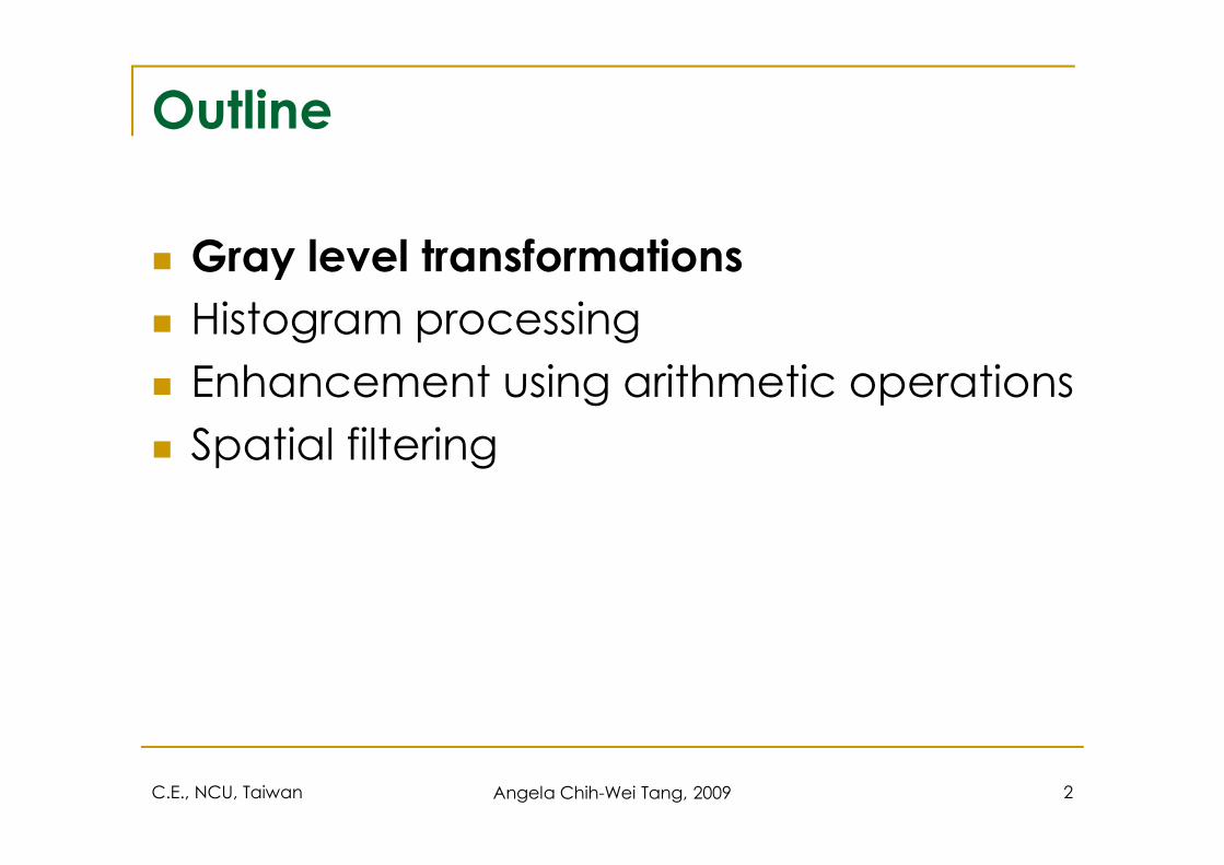
Background
)],([),( yxfTyxg =
� Spatial domain methods
� operate directly on the pixels
� T operates over some neighborhood of (x,y)
� neighborhood shape: square & rectangular arrays are the most predominant due to the ease of implementation
� mask processing/filtering
� masks/filters/kernels/templates/windows� masks/filters/kernels/templates/windows
� e.g., image sharpening
� the center of the window
moves from pixel to pixel
� the simplest form:
gray-level transformation
� s=T(r)
� T can operate on a set of input images
� e.g., sum of input images for
noise reduction3C.E., NCU, Taiwan 3Angela Chih-Wei Tang, 2009
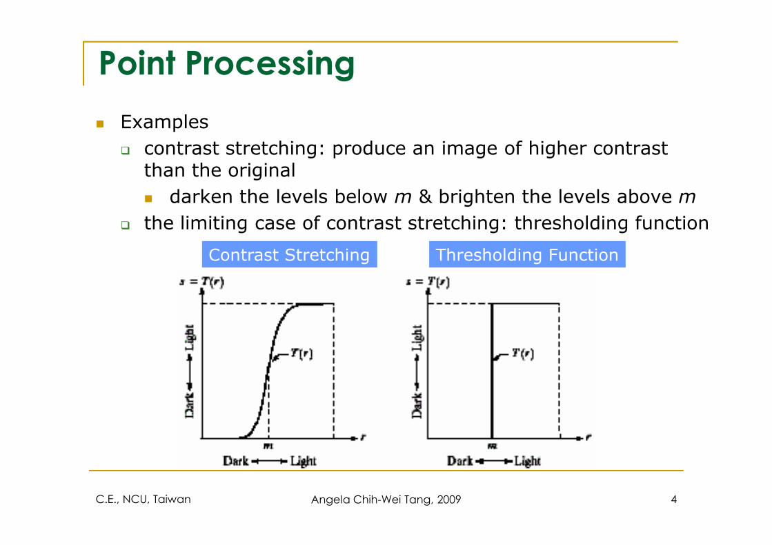
Point Processing
� Examples
� contrast stretching: produce an image of higher contrast than the original
� darken the levels below m & brighten the levels above m
� the limiting case of contrast stretching: thresholding function
Contrast Stretching Thresholding Function
C.E., NCU, Taiwan Angela Chih-Wei Tang, 2009 4
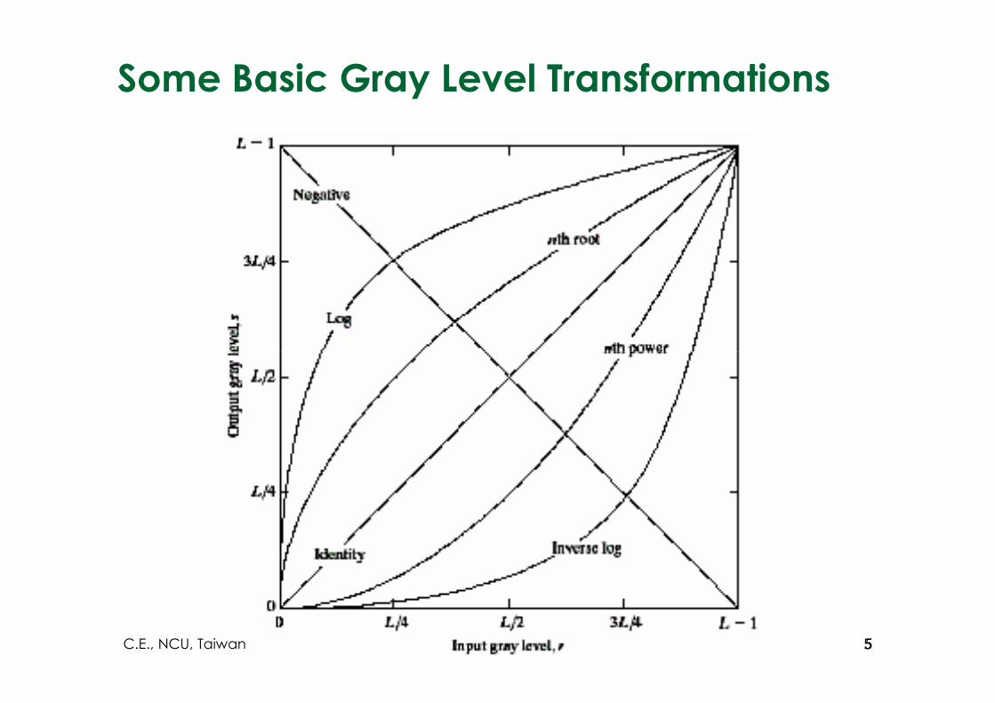
Some Basic Gray Level Transformations
5C.E., NCU, Taiwan 5
Gray Level Transformations –
Image Negatives
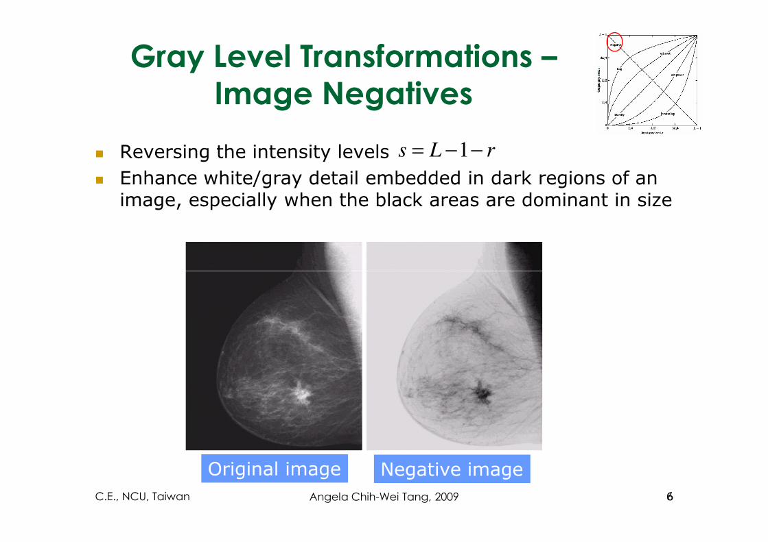
� Reversing the intensity levels
� Enhance white/gray detail embedded in dark regions of an image, especially when the black areas are dominant in size
rLs −−= 1
Original image Negative image
6C.E., NCU, Taiwan 6Angela Chih-Wei Tang, 2009
Gray Level Transformations –
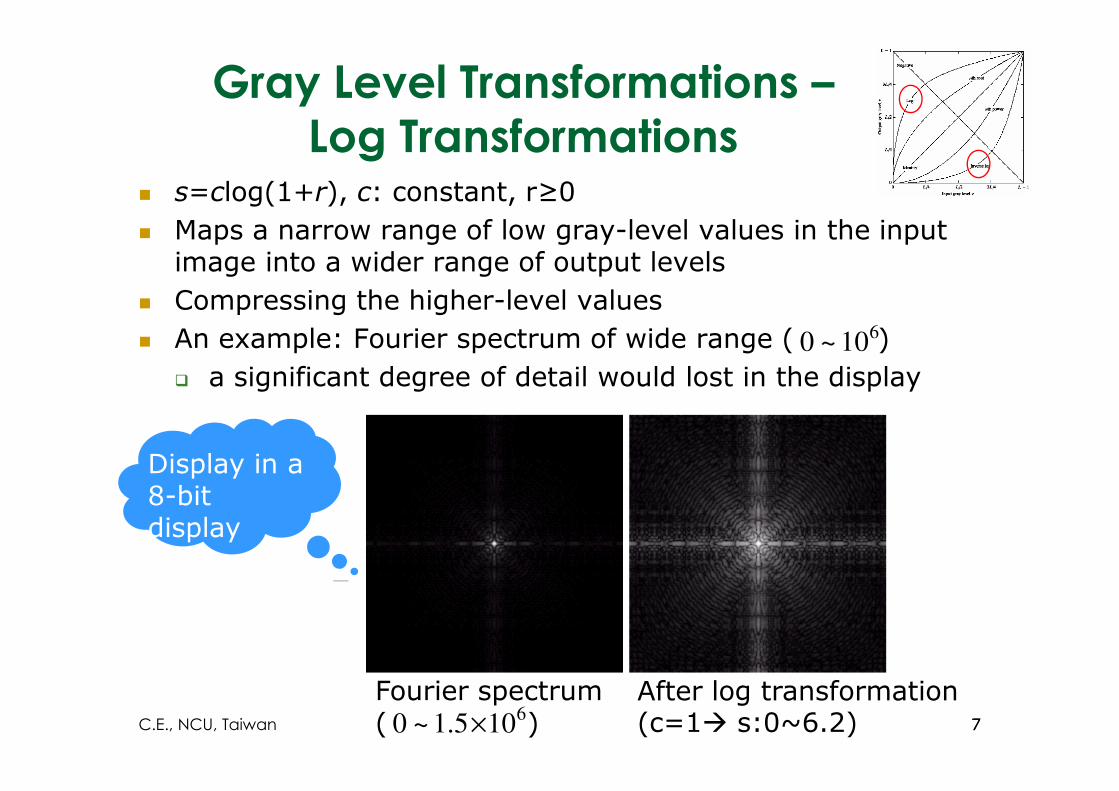
Log Transformations� s=clog(1+r), c: constant, r≥0
� Maps a narrow range of low gray-level values in the input image into a wider range of output levels
� Compressing the higher-level values
� An example: Fourier spectrum of wide range ( )
� a significant degree of detail would lost in the display
610~0
Fourier spectrum( )
After log transformation(c=1� s:0~6.2)6
105.1~0 ×
Display in a 8-bit display
7C.E., NCU, Taiwan 7
Gray Level Transformations –
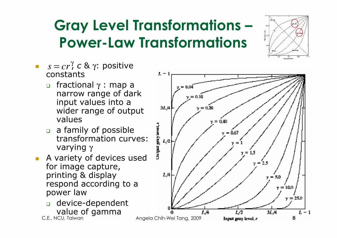
Power-Law Transformations
� , c & γ: positive constants
� fractional γ : map a narrow range of dark input values into a wider range of output values
γ= crs
values
� a family of possible transformation curves: varying γ
� A variety of devices used for image capture, printing & display respond according to a power law
� device-dependent value of gamma
8C.E., NCU, Taiwan 8Angela Chih-Wei Tang, 2009
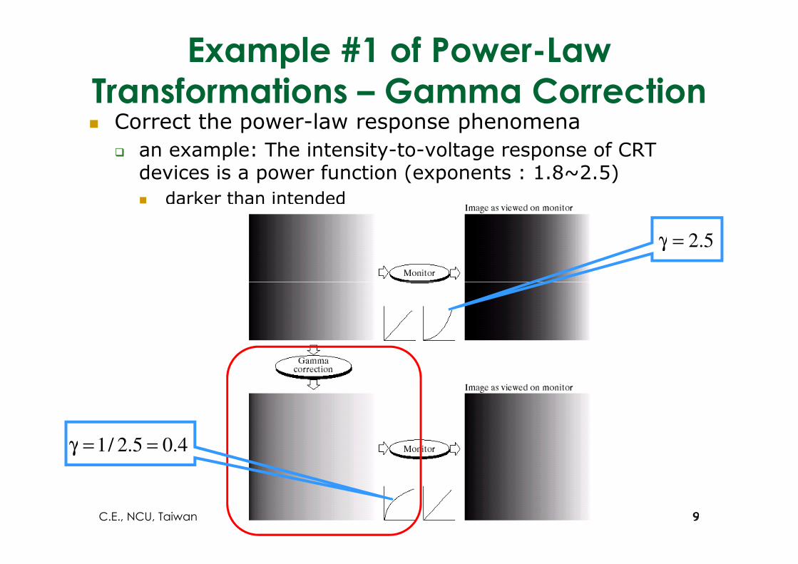
Example #1 of Power-Law
Transformations – Gamma Correction� Correct the power-law response phenomena
� an example: The intensity-to-voltage response of CRT devices is a power function (exponents : 1.8~2.5)
� darker than intended
5.2=γ
4.05.2/1 ==γ
9C.E., NCU, Taiwan 9
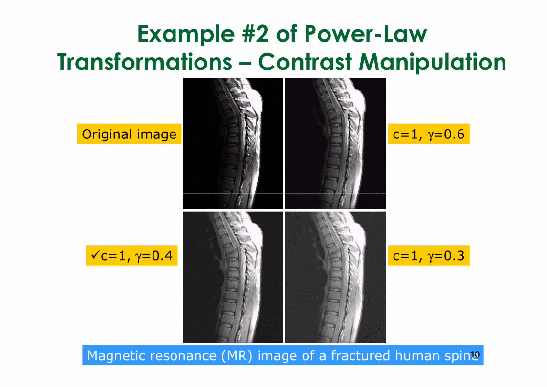
Example #2 of Power-Law
Transformations – Contrast Manipulation
Original image c=1, γ=0.6
Magnetic resonance (MR) image of a fractured human spine
�c=1, γ=0.4 c=1, γ=0.3
1010
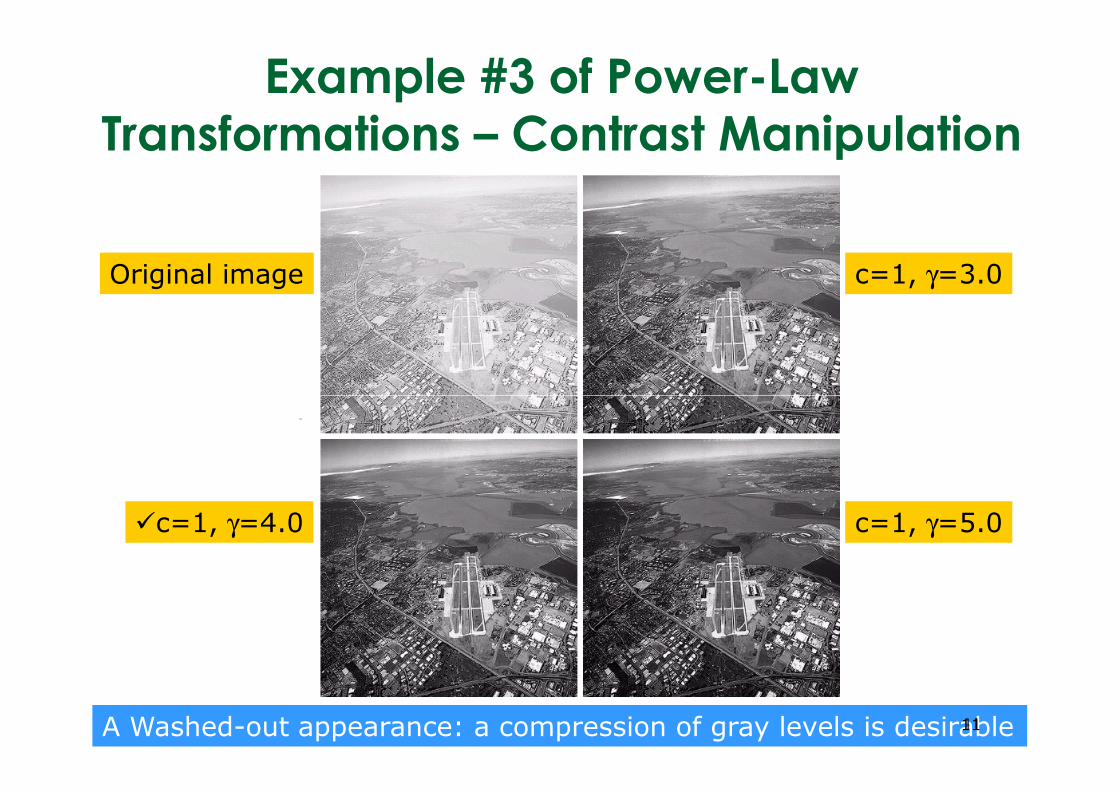
Example #3 of Power-Law
Transformations – Contrast Manipulation
Original image c=1, γ=3.0
A Washed-out appearance: a compression of gray levels is desirable
�c=1, γ=4.0 c=1, γ=5.0
1111
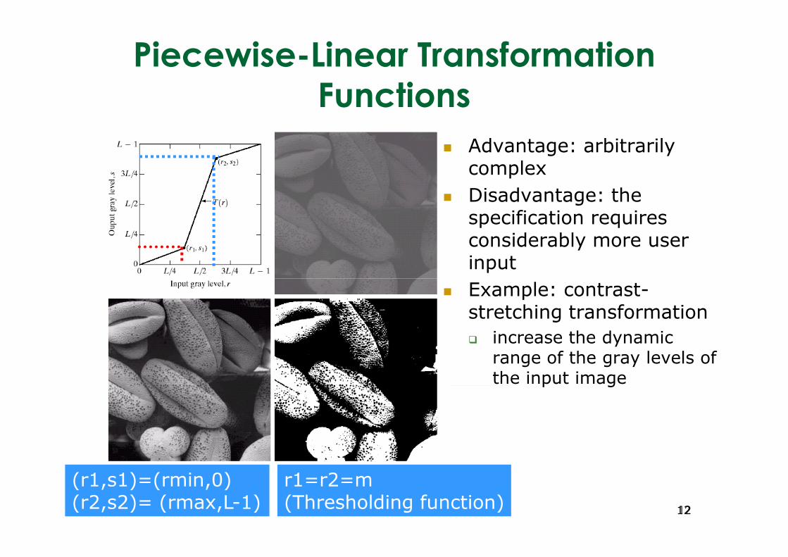
Piecewise-Linear Transformation
Functions
� Advantage: arbitrarily complex
� Disadvantage: the specification requires considerably more user input
Example: contrast-� Example: contrast-stretching transformation
� increase the dynamic range of the gray levels of the input image
r1=r2=m (Thresholding function)
(r1,s1)=(rmin,0)(r2,s2)= (rmax,L-1) 1212
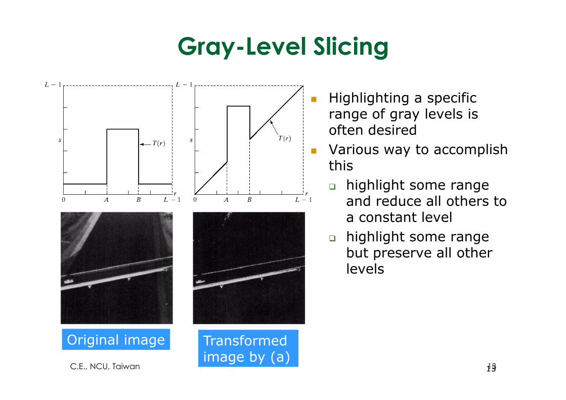
Gray-Level Slicing
� Highlighting a specific range of gray levels is often desired
� Various way to accomplish this
� highlight some range and reduce all others to and reduce all others to a constant level
� highlight some range but preserve all other levels
Original image Transformed image by (a)
13C.E., NCU, Taiwan 13
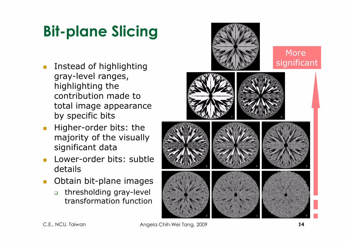
Bit-plane Slicing
� Instead of highlighting gray-level ranges, highlighting the contribution made to total image appearance by specific bits
Higher-order bits: the
More significant
More significant
� Higher-order bits: the majority of the visually significant data
� Lower-order bits: subtle details
� Obtain bit-plane images
� thresholding gray-level transformation function
14C.E., NCU, Taiwan 14Angela Chih-Wei Tang, 2009
Outline
� Gray level transformations
� Histogram processing
� Enhancement using arithmetic operations
C.E., NCU, Taiwan Angela Chih-Wei Tang, 2009 15
� Spatial filtering
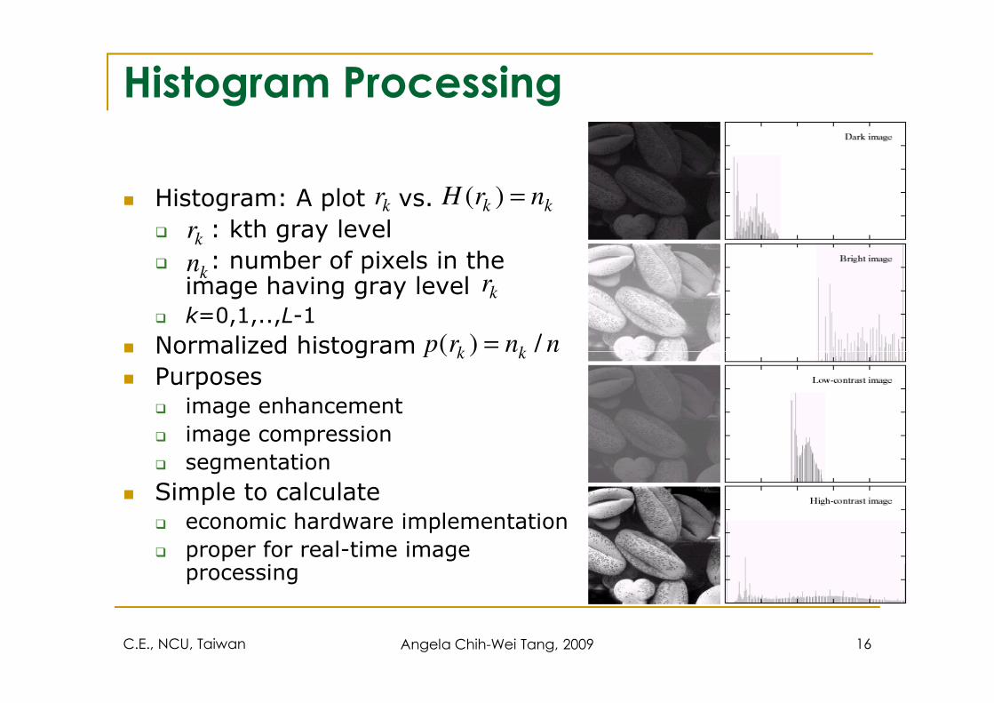
Histogram Processing
� Histogram: A plot vs.
� : kth gray level
� : number of pixels in the image having gray level
� k=0,1,..,L-1
� Normalized histogram
kr kk nrH =)(
kr
knkr
nnrp kk /)( =
C.E., NCU, Taiwan Angela Chih-Wei Tang, 2009 16
� Normalized histogram
� Purposes� image enhancement
� image compression
� segmentation
� Simple to calculate� economic hardware implementation
� proper for real-time image processing
nnrp kk /)( =
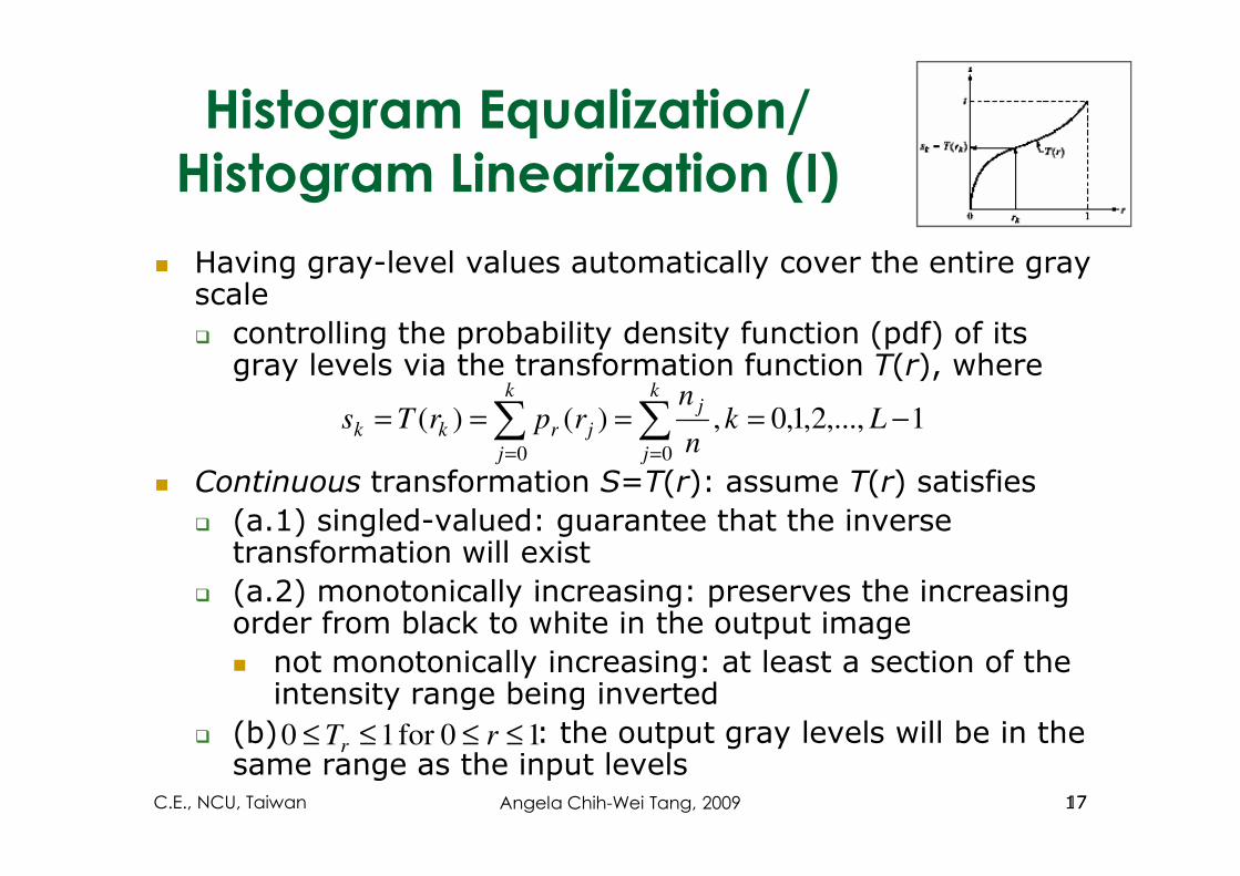
Histogram Equalization/
Histogram Linearization (I)
� Having gray-level values automatically cover the entire gray scale
� controlling the probability density function (pdf) of its gray levels via the transformation function T(r), where
∑ ∑ −====k k
j
jrkk Lkn
nrprTs 1,...,2,1,0,)()(
� Continuous transformation S=T(r): assume T(r) satisfies
� (a.1) singled-valued: guarantee that the inverse transformation will exist
� (a.2) monotonically increasing: preserves the increasing order from black to white in the output image
� not monotonically increasing: at least a section of the intensity range being inverted
� (b) : the output gray levels will be in the same range as the input levels
∑ ∑= =j j
jrkkn0 0
10for 10 ≤≤≤≤ rTr
17C.E., NCU, Taiwan 17Angela Chih-Wei Tang, 2009
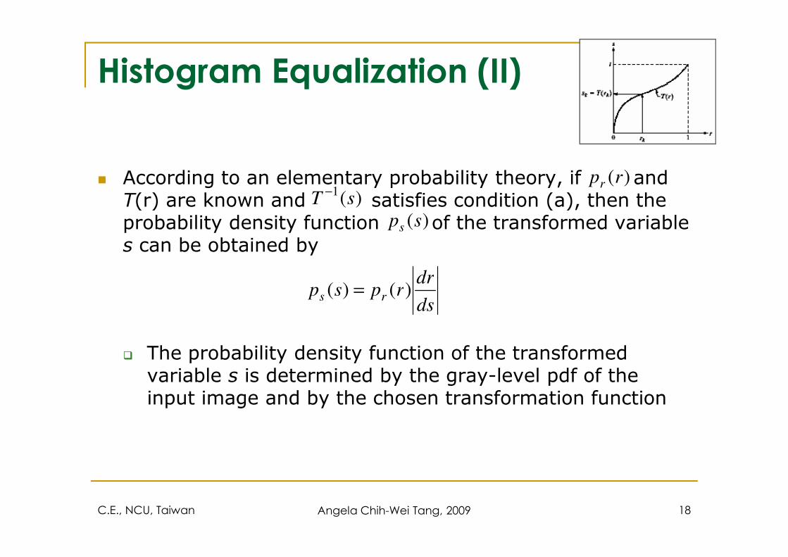
Histogram Equalization (II)
� According to an elementary probability theory, if and T(r) are known and satisfies condition (a), then the probability density function of the transformed variable s can be obtained by
drrpsp )()( =
)(sps
)(rpr
)(1
sT−
C.E., NCU, Taiwan Angela Chih-Wei Tang, 2009 18
� The probability density function of the transformed variable s is determined by the gray-level pdf of the input image and by the chosen transformation function
ds
drrpsp rs )()( =
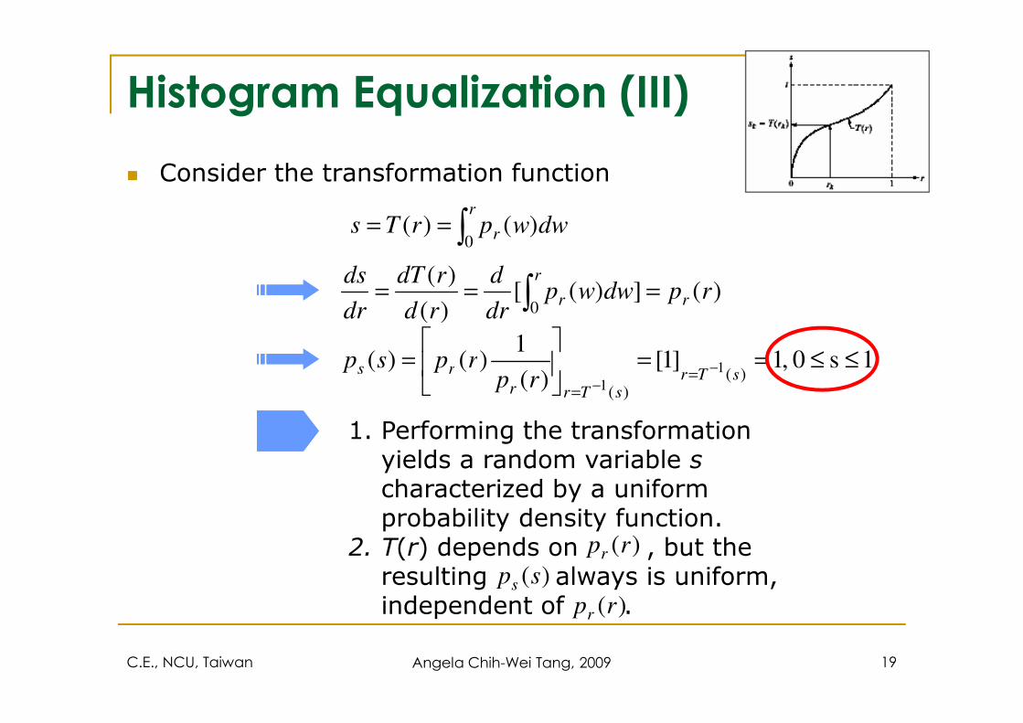
Histogram Equalization (III)
� Consider the transformation function
∫==r
r dwwprTs0
)()(
)(])([)(
)(
0rpdwwp
dr
d
rd
rdT
dr
dsr
r
r === ∫
1s0 ,1]1[1
)()( 1 ≤≤==
= −rs rpsp
C.E., NCU, Taiwan Angela Chih-Wei Tang, 2009 19
1s0 ,1]1[)(
)()()(
)(
1
1
≤≤==
= −−
==
sTrsTrr
rsrp
rpsp
1. Performing the transformation yields a random variable scharacterized by a uniform probability density function.
2. T(r) depends on , but the resulting always is uniform, independent of .
)(rpr
)(sps
)(rpr
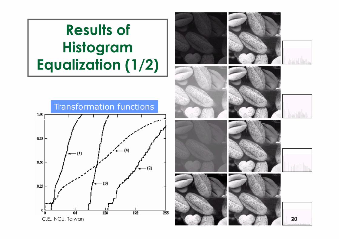
Results of
Histogram
Equalization (1/2)
Transformation functions
20C.E., NCU, Taiwan 20
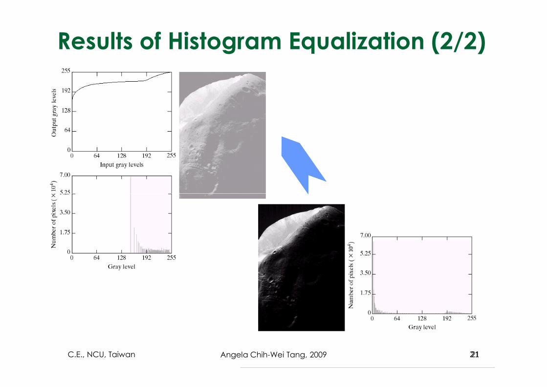
Results of Histogram Equalization (2/2)
21C.E., NCU, Taiwan 21Angela Chih-Wei Tang, 2009
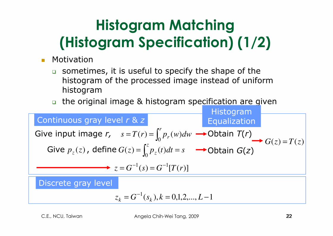
Histogram Matching
(Histogram Specification) (1/2)� Motivation
� sometimes, it is useful to specify the shape of the histogram of the processed image instead of uniform histogram
� the original image & histogram specification are given
Continuous gray level r & zHistogram
Equalization
∫==r
r dwwprTs0
)()(
sdttpzGz
z == ∫0 )()(, define
)]([)(11
rTGsGz−− ==
)()( zTzG =Obtain T(r)
Obtain G(z))(zpzGive
Give input image r,
Continuous gray level r & z
Discrete gray level
1,...,2,1,0),(1 −== −
LksGz kk
Equalization
22C.E., NCU, Taiwan 22Angela Chih-Wei Tang, 2009
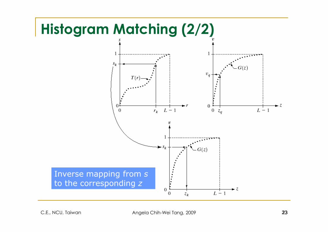
Histogram Matching (2/2)
C.E., NCU, Taiwan Angela Chih-Wei Tang, 2009 23
Inverse mapping from sto the corresponding z
23
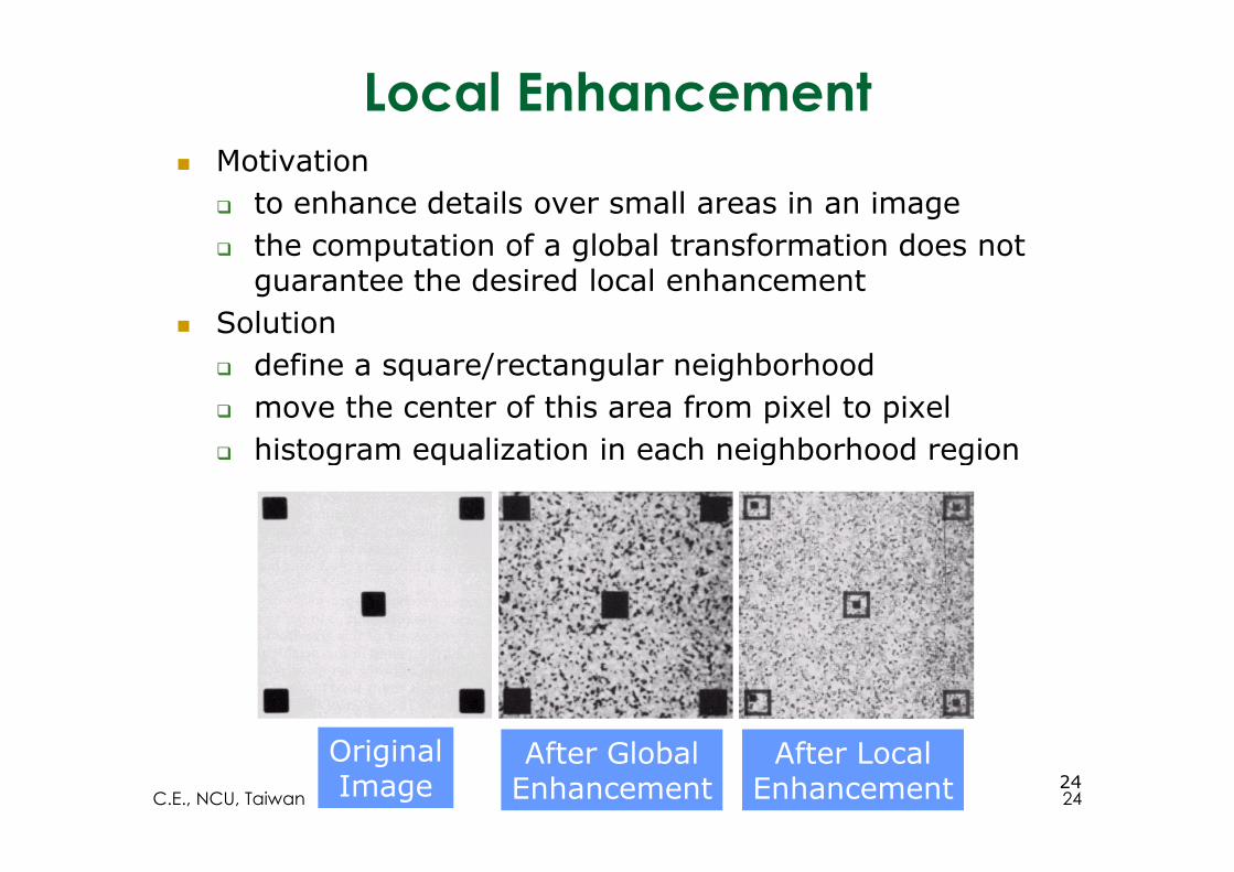
Local Enhancement� Motivation
� to enhance details over small areas in an image
� the computation of a global transformation does not guarantee the desired local enhancement
� Solution
� define a square/rectangular neighborhood
� move the center of this area from pixel to pixel
histogram equalization in each neighborhood region� histogram equalization in each neighborhood region
OriginalImage
After GlobalEnhancement
After LocalEnhancement 24
C.E., NCU, Taiwan 24
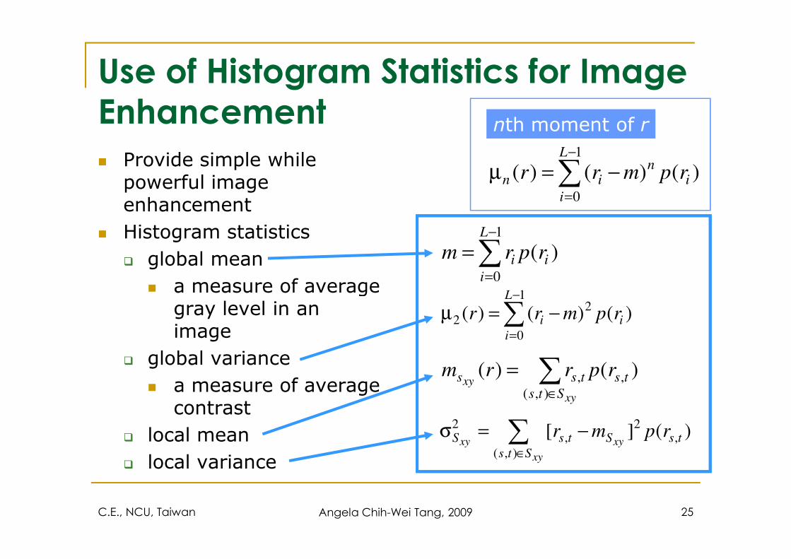
Use of Histogram Statistics for Image
Enhancement
� Provide simple while powerful image enhancement
� Histogram statistics
� global mean
a measure of average
∑−
=
=1
0
)(L
i
ii rprm
∑−
=
−=µ1
0
)()()(L
i
in
in rpmrr
nth moment of r
C.E., NCU, Taiwan Angela Chih-Wei Tang, 2009 25
� a measure of average gray level in an image
� global variance
� a measure of average contrast
� local mean
� local variance
=0i
∑−
=
−=µ1
0
22 )()()(
L
i
ii rpmrr
∑∈
=xy
xySts
tstss rprrm),(
,, )()(
∑∈
−=σxy
xyxySts
tsStsS rpmr),(
,2
,2
)(][
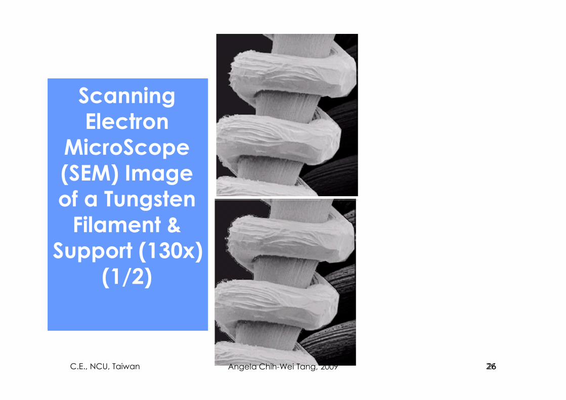
Scanning
Electron
MicroScope
(SEM) Image
of a Tungsten
Support (130x)
of a Tungsten
Filament &
Support (130x)
(1/2)
26C.E., NCU, Taiwan 26Angela Chih-Wei Tang, 2009
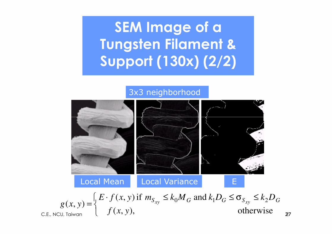
SEM Image of a
Tungsten Filament &
Support (130x) (2/2)
3x3 neighborhood3x3 neighborhood
≤σ≤≤⋅
=otherwise ),,(
and if ),(),(
210
yxf
DkDkMkmyxfEyxg
GSGGS xyxy
Local MeanLocal Mean Local VarianceLocal Variance EE
27C.E., NCU, Taiwan 27
Outline
� Gray level transformations
� Histogram processing
� Enhancement using arithmetic operations
C.E., NCU, Taiwan Angela Chih-Wei Tang, 2009 28
� Spatial filtering
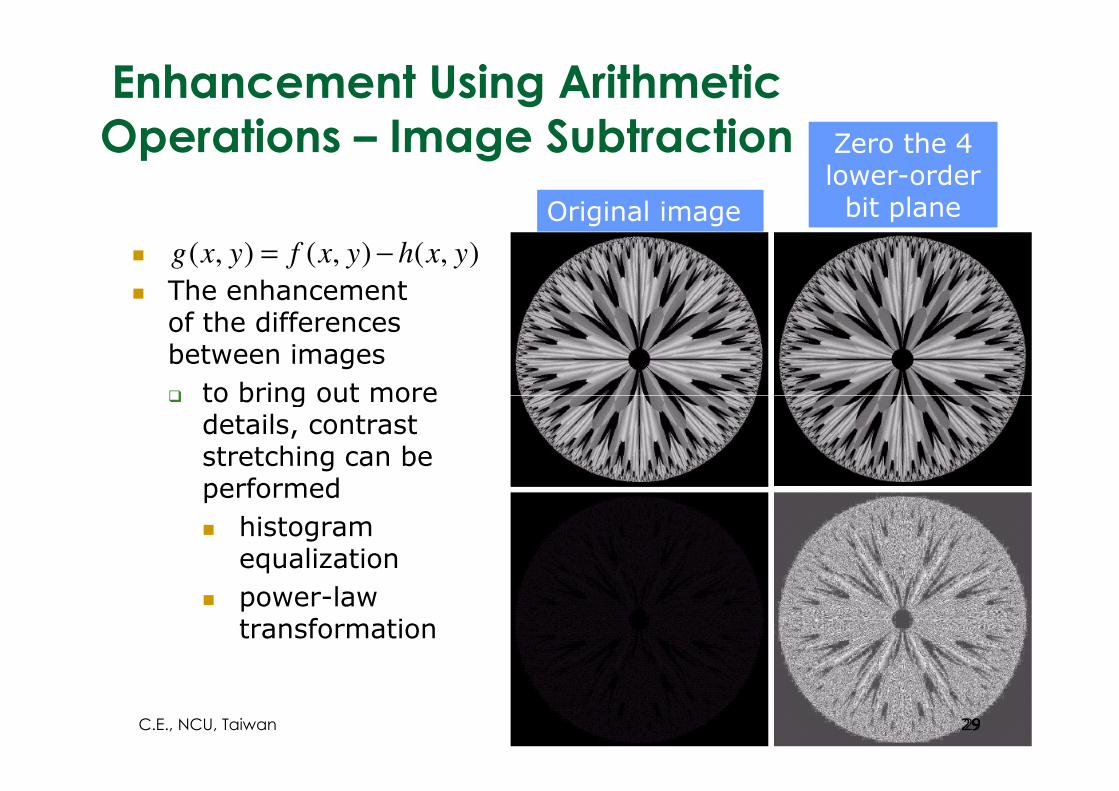
Enhancement Using Arithmetic
Operations – Image Subtraction
�
� The enhancement of the differences between images
� to bring out more
Original imageOriginal image
Zero the 4 lower-order bit plane
Zero the 4 lower-order bit plane
),(),(),( yxhyxfyxg −=
� to bring out more details, contrast stretching can be performed
� histogram equalization
� power-law transformation
29C.E., NCU, Taiwan 29
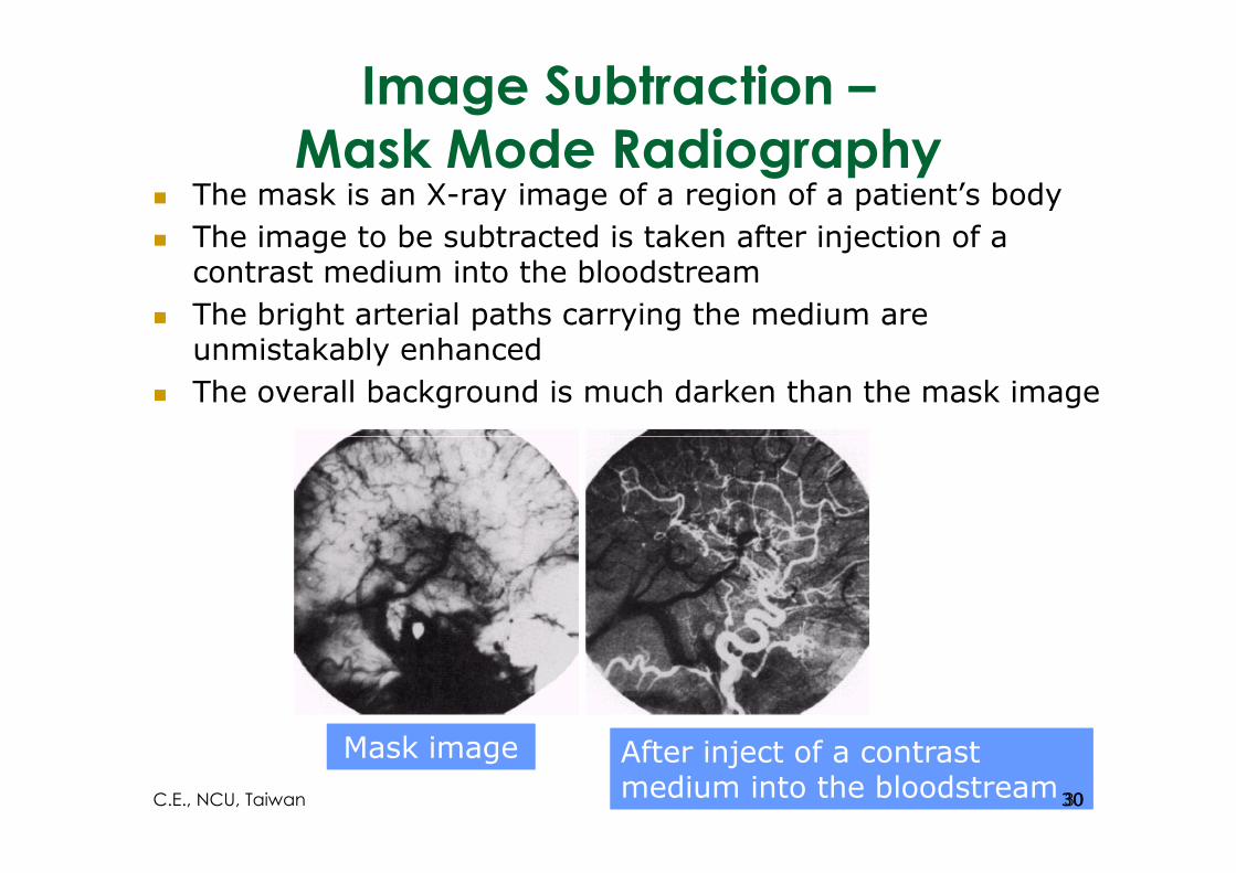
Image Subtraction –
Mask Mode Radiography� The mask is an X-ray image of a region of a patient’s body
� The image to be subtracted is taken after injection of a contrast medium into the bloodstream
� The bright arterial paths carrying the medium are unmistakably enhanced
� The overall background is much darken than the mask image
Mask imageMask image After inject of a contrast medium into the bloodstreamAfter inject of a contrast medium into the bloodstream30C.E., NCU, Taiwan 30
The Range of the Image Values
After Image Subtraction
� For 8-bit image: -255~255
� Two principle ways to scale a different image
� add 255 to every pixel & divide by 2
� limitation: the full range of the display may not be utilized
the value of the minimum difference is obtained & its
C.E., NCU, Taiwan Angela Chih-Wei Tang, 2009 31
� the value of the minimum difference is obtained & its negative added to all the pixels in the difference image
� scale to the interval [0, 255]
� more complex
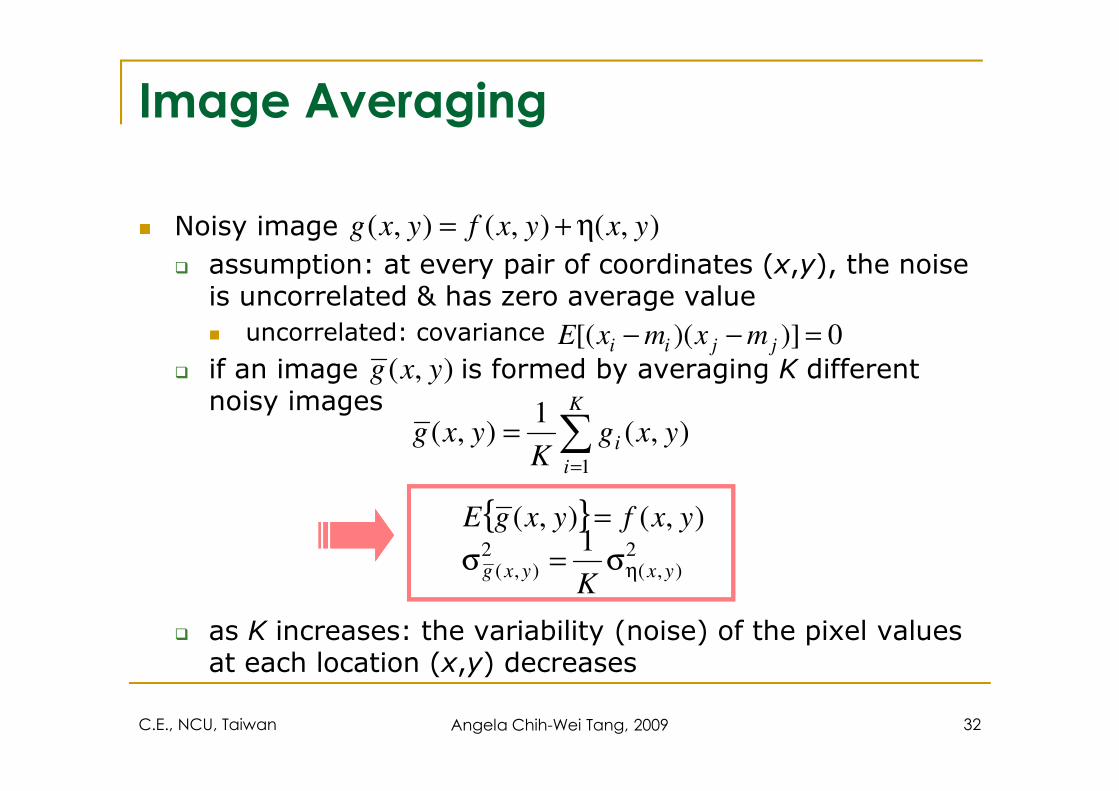
Image Averaging
� Noisy image
� assumption: at every pair of coordinates (x,y), the noise is uncorrelated & has zero average value
� uncorrelated: covariance
� if an image is formed by averaging K different noisy images
),(),(),( yxyxfyxg η+=
0)])([( =−− jjii mxmxE
),( yxgK1
C.E., NCU, Taiwan Angela Chih-Wei Tang, 2009 32
noisy images
� as K increases: the variability (noise) of the pixel values at each location (x,y) decreases
∑=
=K
i
i yxgK
yxg1
),(1
),(
{ } ),(),( yxfyxgE =2
),(2
),(
1yxyxg
Kησ=σ
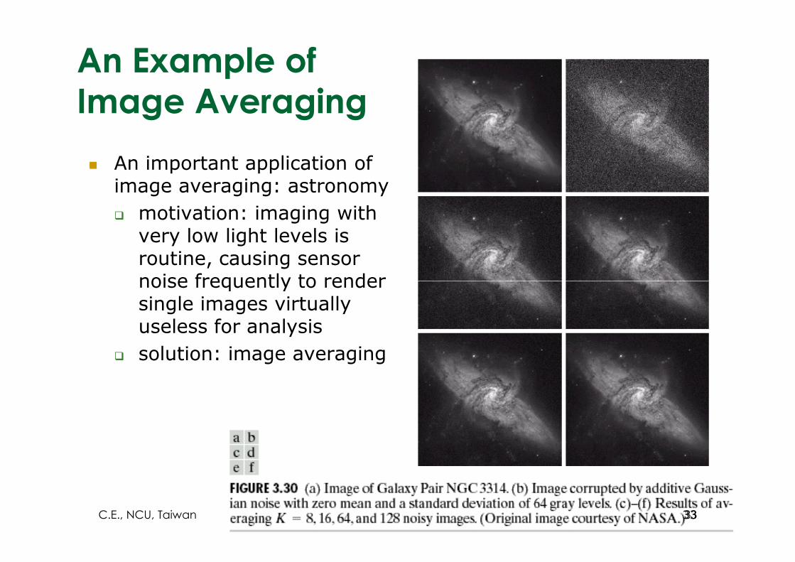
An Example of
Image Averaging
� An important application of image averaging: astronomy
� motivation: imaging with very low light levels is routine, causing sensor noise frequently to render noise frequently to render single images virtually useless for analysis
� solution: image averaging
33C.E., NCU, Taiwan 33
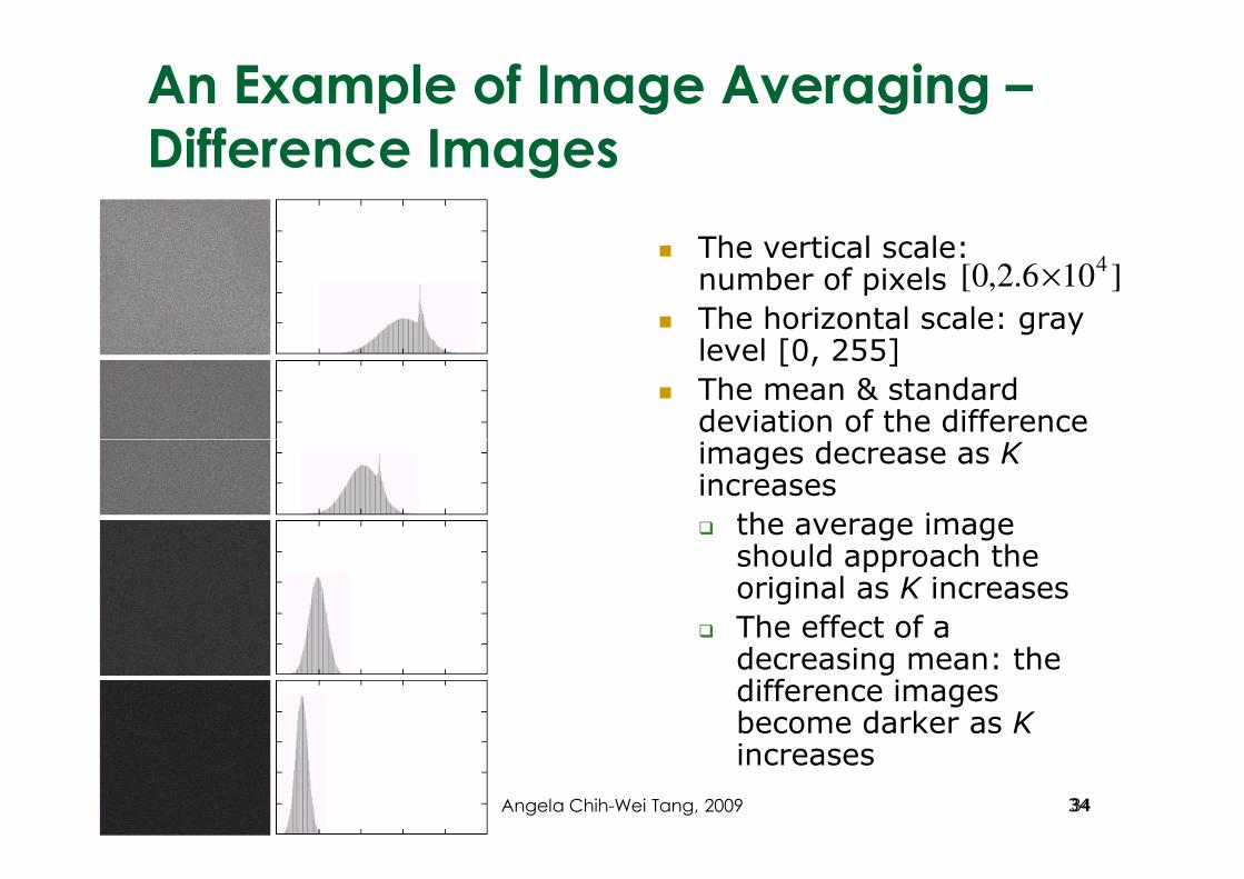
An Example of Image Averaging –
Difference Images
� The vertical scale: number of pixels
� The horizontal scale: gray level [0, 255]
� The mean & standard deviation of the difference images decrease as K
]106.2,0[4×
images decrease as K increases
� the average image should approach the original as K increases
� The effect of a decreasing mean: the difference images become darker as Kincreases
3434Angela Chih-Wei Tang, 2009
Outline
� Gray level transformations
� Histogram processing
� Enhancement using arithmetic operations
C.E., NCU, Taiwan Angela Chih-Wei Tang, 2009 35
� Spatial filtering
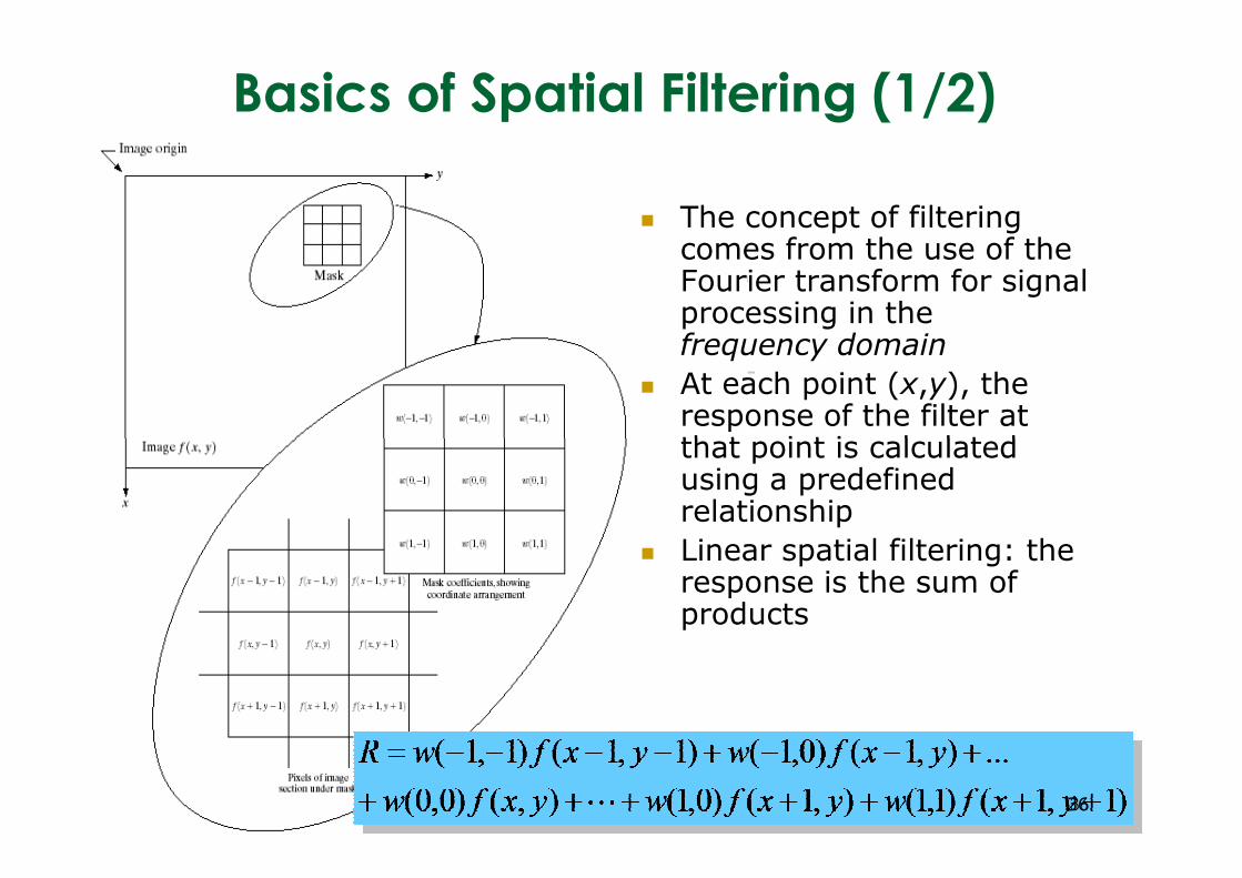
Basics of Spatial Filtering (1/2)
� The concept of filtering comes from the use of the Fourier transform for signal processing in the frequency domain
� At each point (x,y), the response of the filter at that point is calculated that point is calculated using a predefined relationship
� Linear spatial filtering: the response is the sum of products
3636
Basics of Spatial Filtering (2/2)
� Linear spatial filtering often is referred to as “convolving a mask with an image.”
� filtering mask / convolution mask / convolution kernel
� Nonlinear spatial filtering
� the filtering operation is based conditionally on the values of the pixels in the neighborhood under consideration, but not explicitly use coefficients in the
C.E., NCU, Taiwan Angela Chih-Wei Tang, 2009 37
consideration, but not explicitly use coefficients in the sum-of-products manner
� e.g., median filter for noise reduction: compute the median gray-level value in the neighborhood
What Happens When the Center of the Filter
Approaches the Border of the Image ?
� One or more rows/columns of the mask will be located outside the image plane
� Solution
� limit the excursions of the center of the mask to be at a distance no less than (n-1)/2 pixels from the border
� the resulting filtered image is smaller than the original� the resulting filtered image is smaller than the original
� partial filter mask: filter all pixels only with the section of the mask that is fully contained in the image
� Padding
� add rows & columns of 0’s (or other constant gray level), or replicate rows/columns
� the padding is stripped off at the end of the process
� side effect: an effect near the edges that becomes more prevalent as the size of the mask increases
38C.E., NCU, Taiwan 38Angela Chih-Wei Tang, 2009
Smoothing Linear Filters (1/2)
� Averaging filters/low pass filters: replace the value of every pixel in an image by the average of the gray levels of the pixels contained in the neighborhood of the filter mask
� Reduce sharp transitions in gray levels
� side effect: blur edges
Reduce irrelevant detail in an image and get a gross
C.E., NCU, Taiwan Angela Chih-Wei Tang, 2009 39
� Reduce irrelevant detail in an image and get a gross representation of objects of interest
� irrelevant: pixel regions that are small with respect to the size of the filter mask
� Applications
� noise reduction
� smooth false contouring
Smoothing Linear
Filters (2/2)
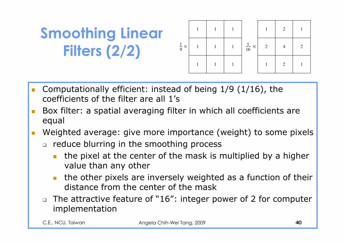
� Computationally efficient: instead of being 1/9 (1/16), the coefficients of the filter are all 1’s
� Box filter: a spatial averaging filter in which all coefficients are equalequal
� Weighted average: give more importance (weight) to some pixels
� reduce blurring in the smoothing process
� the pixel at the center of the mask is multiplied by a higher value than any other
� the other pixels are inversely weighted as a function of their distance from the center of the mask
� The attractive feature of “16”: integer power of 2 for computer implementation
40C.E., NCU, Taiwan 40Angela Chih-Wei Tang, 2009
Examples of Smoothing
Linear Filters (1/2)
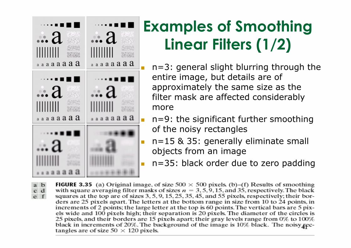
� n=3: general slight blurring through the entire image, but details are of approximately the same size as the filter mask are affected considerably more
� n=9: the significant further smoothing of the noisy rectanglesof the noisy rectangles
� n=15 & 35: generally eliminate small objects from an image
� n=35: black order due to zero padding
4141
Examples of Smoothing Linear Filters (2/2)
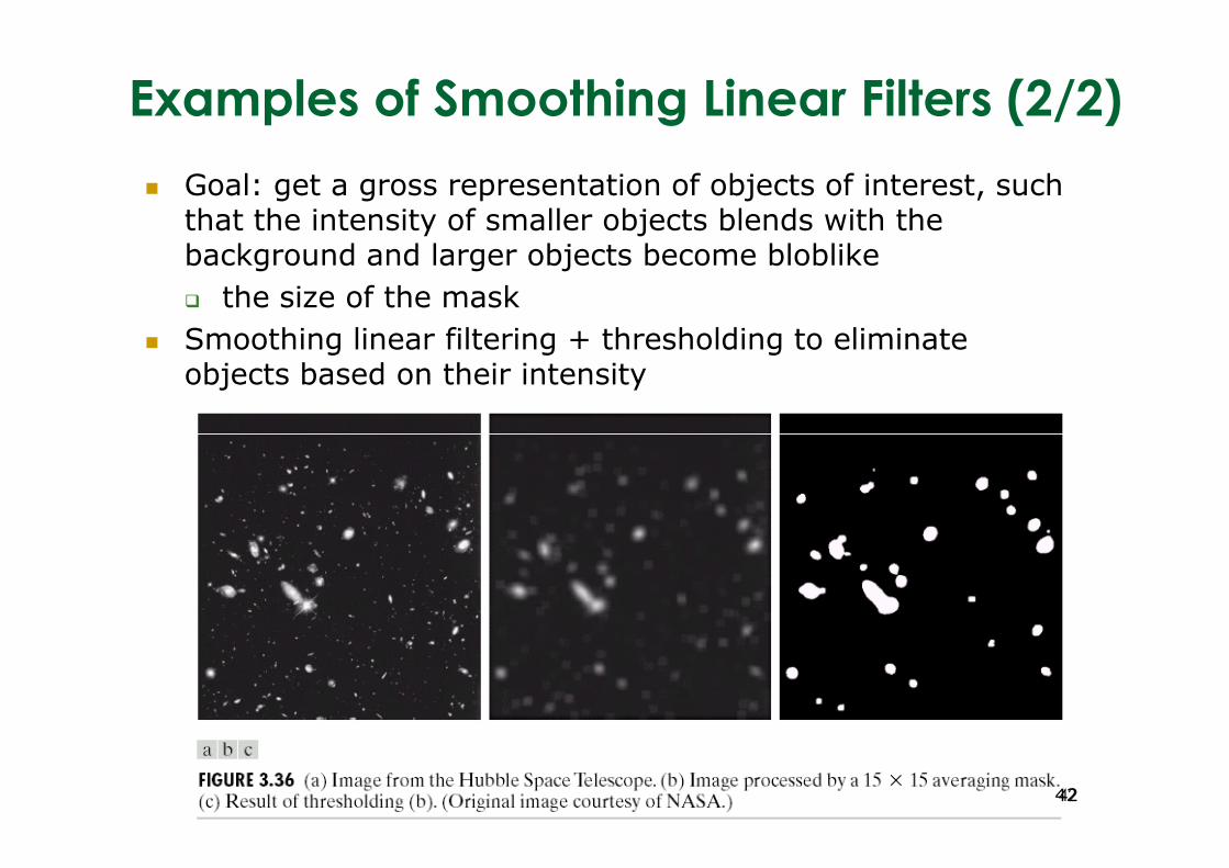
� Goal: get a gross representation of objects of interest, such that the intensity of smaller objects blends with the background and larger objects become bloblike
� the size of the mask
� Smoothing linear filtering + thresholding to eliminate objects based on their intensity
4242
Order-Statistics Filters
� Nonlinear spatial filters whose response is based on ordering (ranking) the pixels in the area to be filtered
� Examples: max filter, min filter & median filter
� Median filter
� replace the value of a pixel by the median of the gray levels in the neighborhood of that pixel
C.E., NCU, Taiwan Angela Chih-Wei Tang, 2009 43
levels in the neighborhood of that pixel� force points with distinct gray levels to be more like their
neighbors
� for 3x3 neighborhood
(10,20,20,20,15,20,20,25,100) -> median is 20
� excellent noise-reduction capabilities, with considerably less blurring than linear smoothing filters of similar size
� particular effective for impulse noise (salt-and-pepper noise
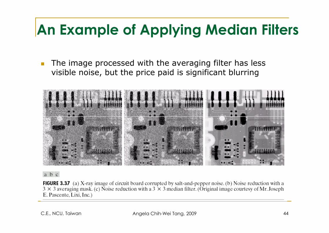
An Example of Applying Median Filters
� The image processed with the averaging filter has less visible noise, but the price paid is significant blurring
C.E., NCU, Taiwan Angela Chih-Wei Tang, 2009 44
Foundations of Sharpening Spatial
Filters (1/2)
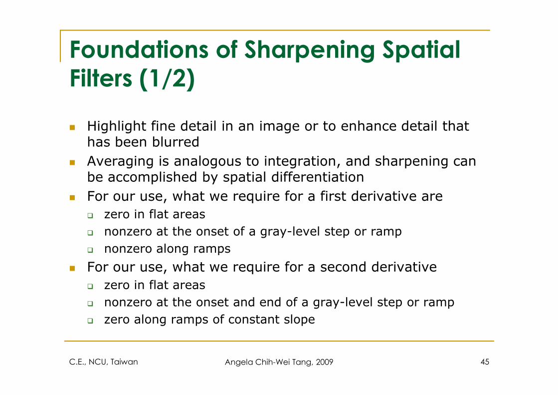
� Highlight fine detail in an image or to enhance detail that has been blurred
� Averaging is analogous to integration, and sharpening can be accomplished by spatial differentiation
� For our use, what we require for a first derivative are
C.E., NCU, Taiwan Angela Chih-Wei Tang, 2009 45
� For our use, what we require for a first derivative are
� zero in flat areas
� nonzero at the onset of a gray-level step or ramp
� nonzero along ramps
� For our use, what we require for a second derivative
� zero in flat areas
� nonzero at the onset and end of a gray-level step or ramp
� zero along ramps of constant slope
Foundations of Sharpening Spatial
Filters (2/2)
� The first-order derivative of a 1-D function f(x)
� The second-order derivative of f(x)
)()1( xfxfx
f−+=
∂
∂
)(2)1()1(2
xfxfxff
−−++=∂
C.E., NCU, Taiwan Angela Chih-Wei Tang, 2009 46
� The two definitions satisfy the conditions stated previously
)(2)1()1(2
xfxfxfx
f−−++=
∂
∂
An Example of Applying Sharpening
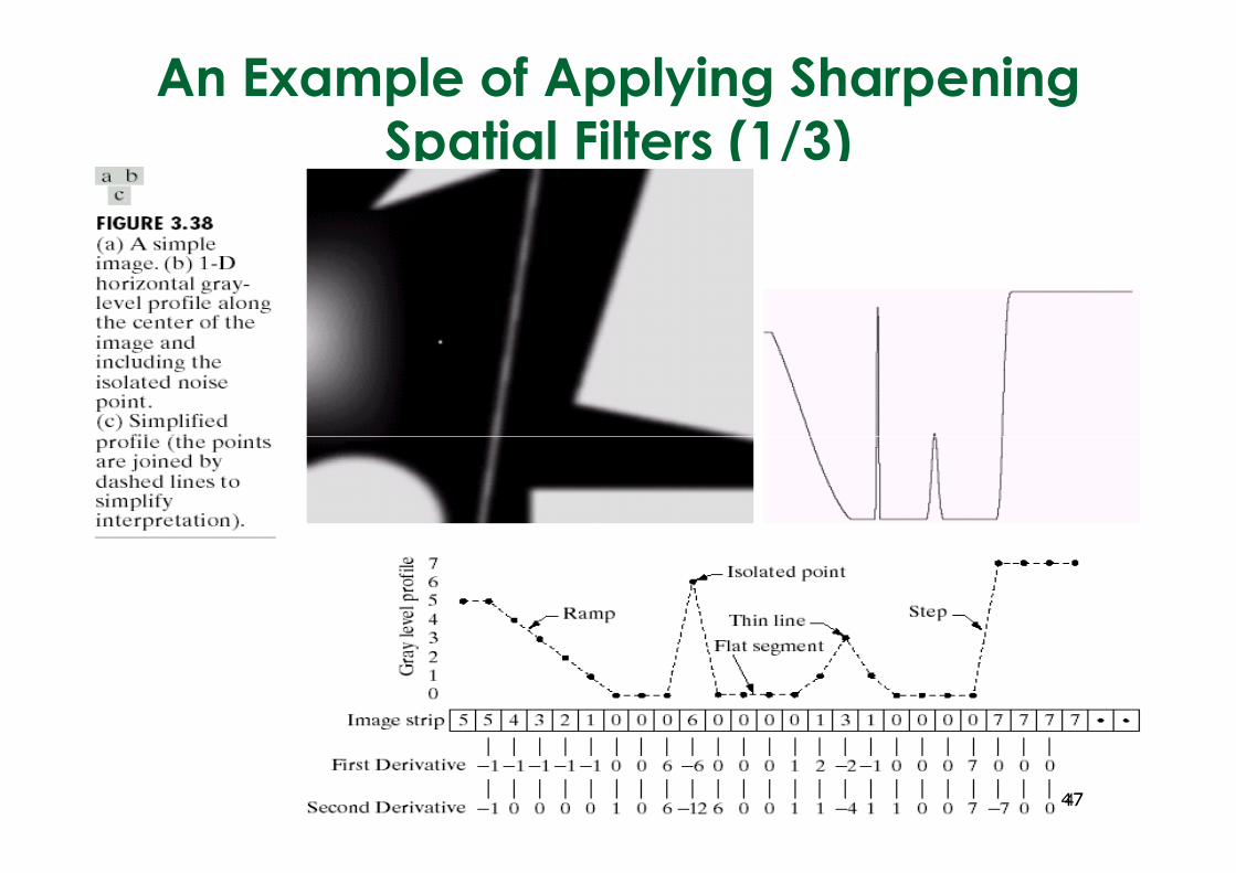
Spatial Filters (1/3)
4747
An Example of Applying Sharpening
Spatial Filters (2/3)� Ramp: the first-order derivative is nonzero along the entire
ramp, while the second-order derivative is nonzero only at the onset and end of the ramp
� first-order derivatives produce thick edges and second-order derivatives, much finer ones
� Isolated noise point: the response at and around the point is much stronger for the second- than for the first-order much stronger for the second- than for the first-order derivative
� second-order derivative enhance much more than a first-order derivative
� Thin line: essentially the same difference between the two derivatives
� Gray-level step:: the response of the two derivatives is the same
� double-edge effect: The second derivative has a transition from positive back to negative 4848
Foundation of
Sharpening Spatial Filters (3/3)
� In most applications, the second derivative is better suited than the first derivative for image enhancement
� The principle use of first derivatives in image processing: edge extraction
C.E., NCU, Taiwan Angela Chih-Wei Tang, 2009 49
Second Derivatives for
Enhancement – The Laplacian
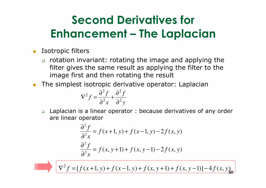
� Isotropic filters
� rotation invariant: rotating the image and applying the filter gives the same result as applying the filter to the image first and then rotating the result
� The simplest isotropic derivative operator: Laplacian
fff
222 ∂
+∂
=∇
� Laplacian is a linear operator : because derivatives of any order are linear operator
y
f
x
ff
22
2
∂
∂+
∂
∂=∇
),(2)1,()1,(
),(2),1(),1(
2
2
2
2
yxfyxfyxfx
f
yxfyxfyxfx
f
−−++=∂
∂
−−++=∂
∂
),(4)]1,()1,(),1(),1([2
yxfyxfyxfyxfyxff −−+++−++=∇5050
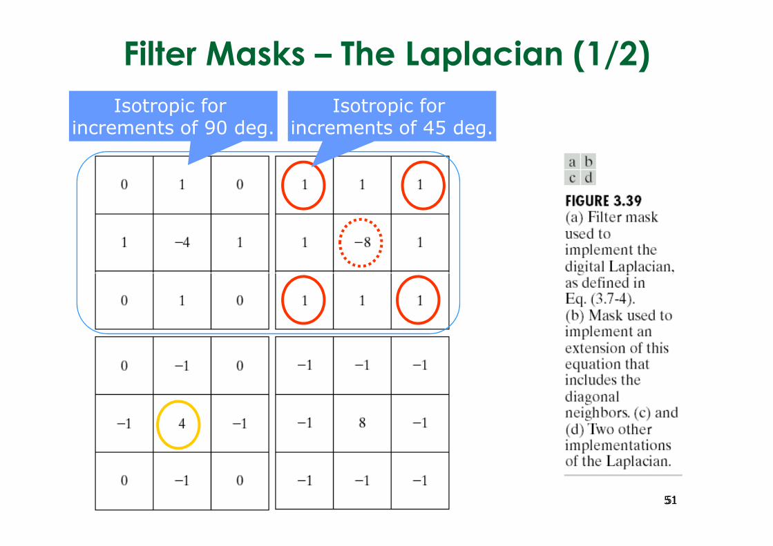
Filter Masks – The Laplacian (1/2)
Isotropic for increments of 45 deg.
Isotropic for increments of 90 deg.
5151
Filter Masks – The Laplacian (2/2)
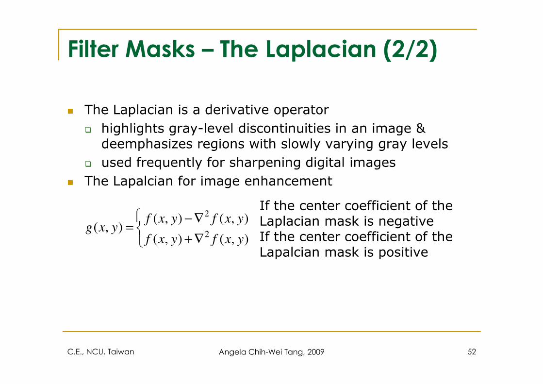
� The Laplacian is a derivative operator
� highlights gray-level discontinuities in an image & deemphasizes regions with slowly varying gray levels
� used frequently for sharpening digital images
� The Lapalcian for image enhancement
C.E., NCU, Taiwan Angela Chih-Wei Tang, 2009 52
∇+
∇−=
),(),(
),(),(),(
2
2
yxfyxf
yxfyxfyxg
If the center coefficient of theLaplacian mask is negativeIf the center coefficient of the Lapalcian mask is positive
Examples of the Laplacian
Enhanced Image (1/2)
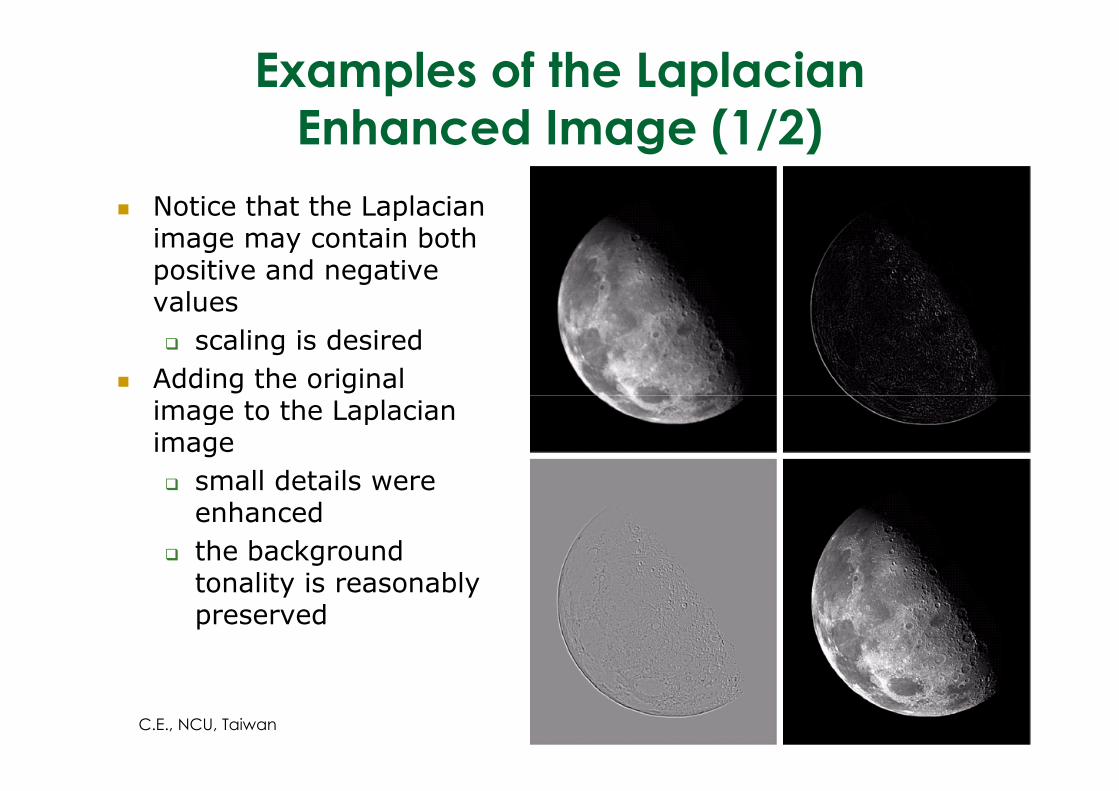
� Notice that the Laplacian image may contain both positive and negative values
� scaling is desired
� Adding the original image to the Laplacian image to the Laplacian image
� small details were enhanced
� the background tonality is reasonably preserved
53C.E., NCU, Taiwan 53
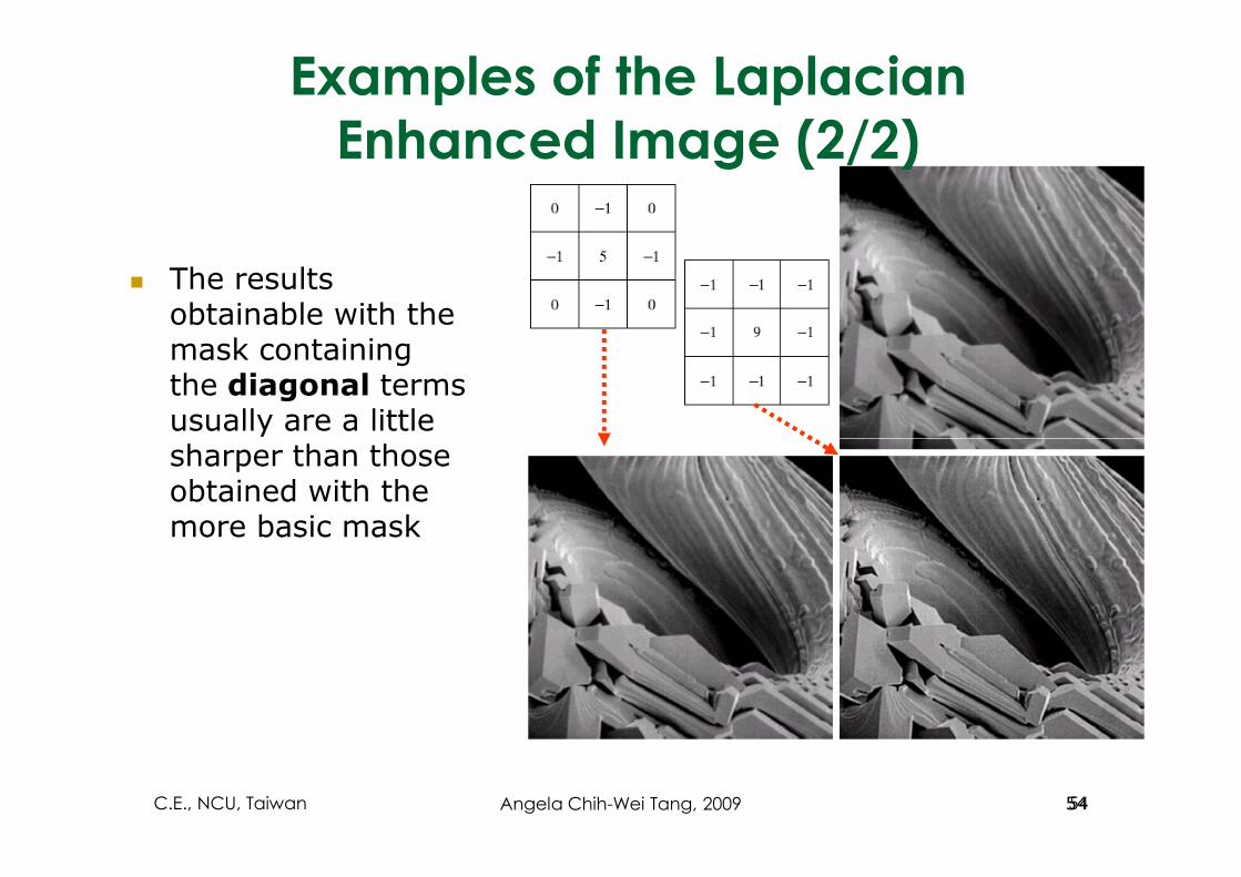
� The results obtainable with the mask containing the diagonal terms usually are a little sharper than those
Examples of the Laplacian
Enhanced Image (2/2)
sharper than those obtained with the more basic mask
54C.E., NCU, Taiwan 54Angela Chih-Wei Tang, 2009
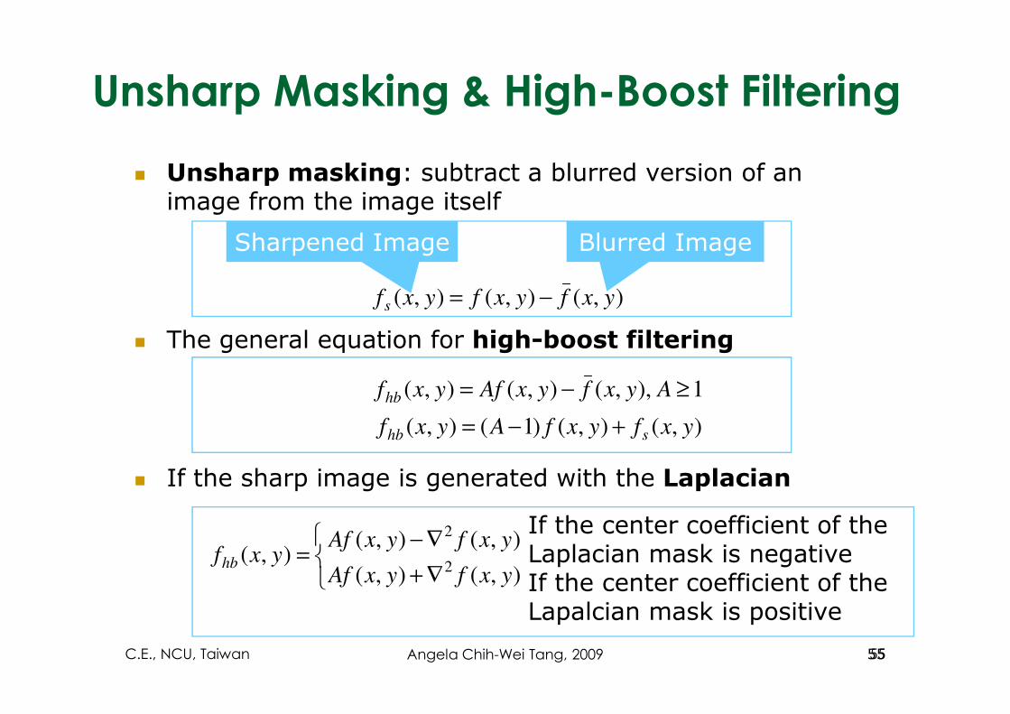
Unsharp Masking & High-Boost Filtering
� Unsharp masking: subtract a blurred version of an image from the image itself
� The general equation for high-boost filtering
),(),(),( yxfyxfyxfs −=
Sharpened Image Blurred Image
� If the sharp image is generated with the Laplacian
1 ),,(),(),( ≥−= AyxfyxAfyxfhb
),(),()1(),( yxfyxfAyxf shb +−=
∇+
∇−=
),(),(
),(),(),(
2
2
yxfyxAf
yxfyxAfyxfhb
If the center coefficient of theLaplacian mask is negativeIf the center coefficient of the Lapalcian mask is positive
55C.E., NCU, Taiwan 55Angela Chih-Wei Tang, 2009
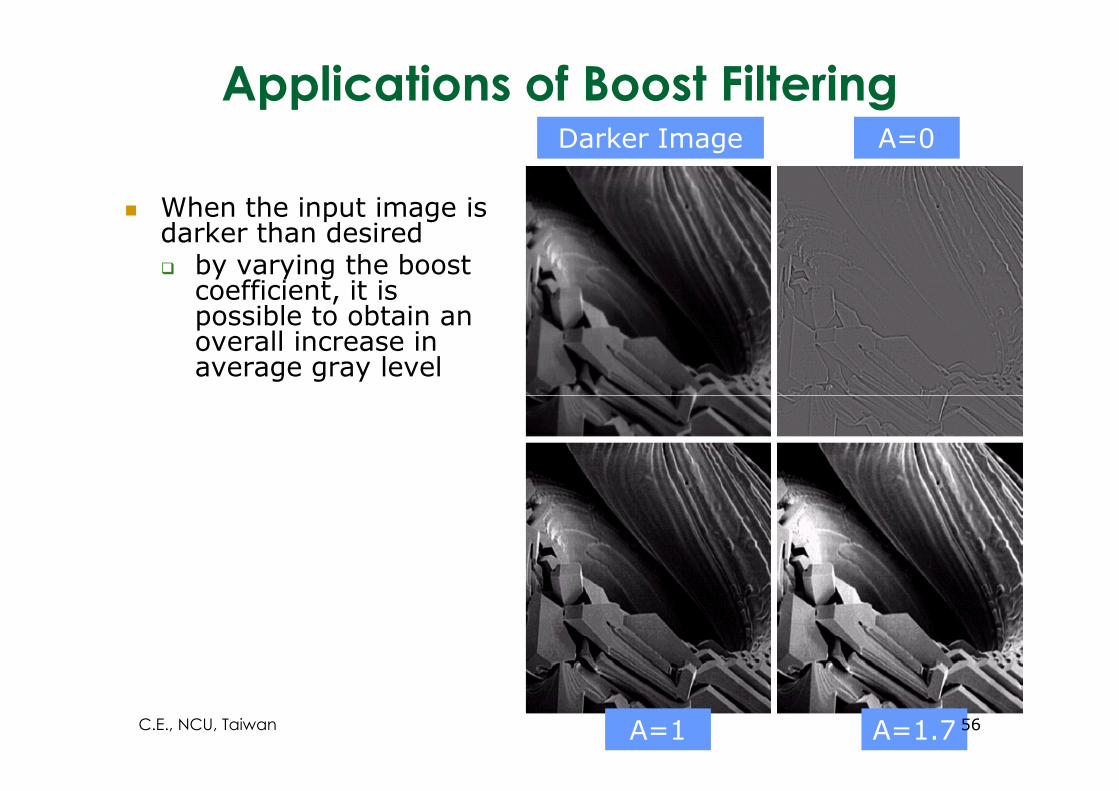
Applications of Boost Filtering
� When the input image is darker than desired� by varying the boost
coefficient, it is possible to obtain an overall increase in average gray level
A=0 A=0 Darker ImageDarker Image
A=1A=1 A=1.7A=1.7 56C.E., NCU, Taiwan
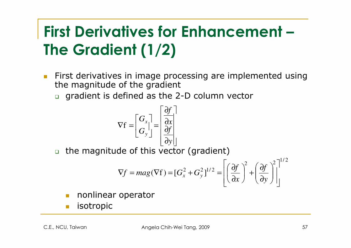
First Derivatives for Enhancement –
The Gradient (1/2)
� First derivatives in image processing are implemented using the magnitude of the gradient
� gradient is defined as the 2-D column vector
∂∂
∂
=
=∇ x
fGx
f
C.E., NCU, Taiwan Angela Chih-Wei Tang, 2009 57
� the magnitude of this vector (gradient)
� nonlinear operator
� isotropic
∂
∂∂=
=∇
y
fx
Gy
xf
2/122
2/122][)f(
∂
∂+
∂
∂=+=∇=∇
y
f
x
fGGmagf yx
First Derivatives for Enhancement –
The Gradient (2/2)
� Problem: the computational burden of implementing the gradient
� The approximation of the magnitude of the gradient
� the isotropic properties of the digital gradient are preserved
yx GG +≈∇f
� the isotropic properties of the digital gradient are preserved only for a limited number of rotational increments (90 deg.)
� Digital approximation of the gradient
5658 , zzGzzG yx −=−=
6859 , zzGzzG yx −=−=
1
2
58C.E., NCU, Taiwan 58Angela Chih-Wei Tang, 2009
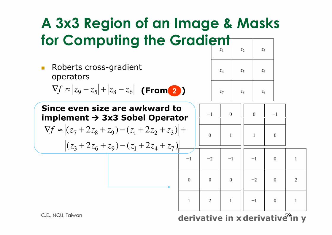
� Roberts cross-gradient operators
6859 zzzzf −+−≈∇ (From )2
Since even size are awkward toimplement ���� 3x3 Sobel Operator
A 3x3 Region of an Image & Masks
for Computing the Gradient
)2()2(
)2()2(
741963
321987
zzzzzz
zzzzzzf
++−++
+++−++≈∇
implement ���� 3x3 Sobel Operator
derivative in xderivative in y59C.E., NCU, Taiwan
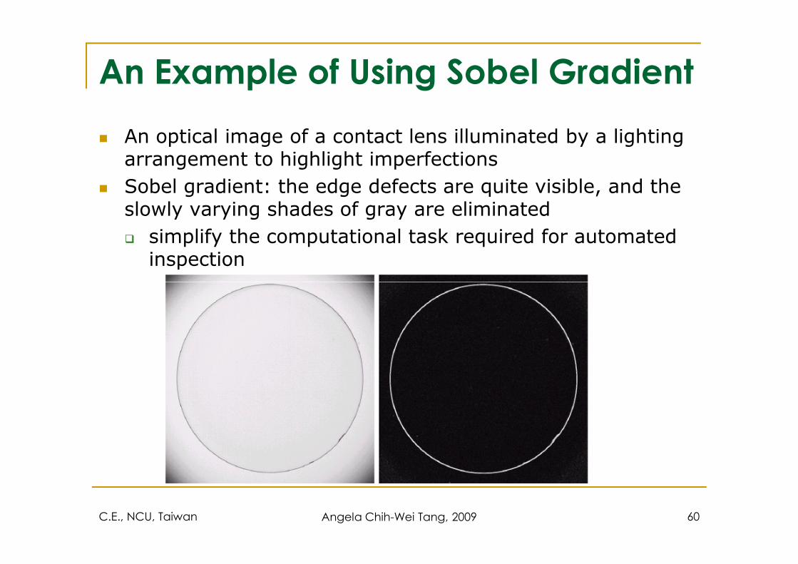
An Example of Using Sobel Gradient
� An optical image of a contact lens illuminated by a lighting arrangement to highlight imperfections
� Sobel gradient: the edge defects are quite visible, and the slowly varying shades of gray are eliminated
� simplify the computational task required for automated inspection
C.E., NCU, Taiwan Angela Chih-Wei Tang, 2009 60