SÄHKÖ- JA TIETOTEKNIIKAN OSASTO SÄHKÖTEKNIIKAN KOULUTUSOHJELMA

IMPLEMENTATION OF FREQUENCY HOPPING CODE PHASE SYNCHRONIZATION METHOD FOR AD HOC NETWORKS

Thesis author __________________________________ Juha Huovinen

Thesis supervisor __________________________________

Jari Iinatti Approved _______/_______2008 Grade __________________________________

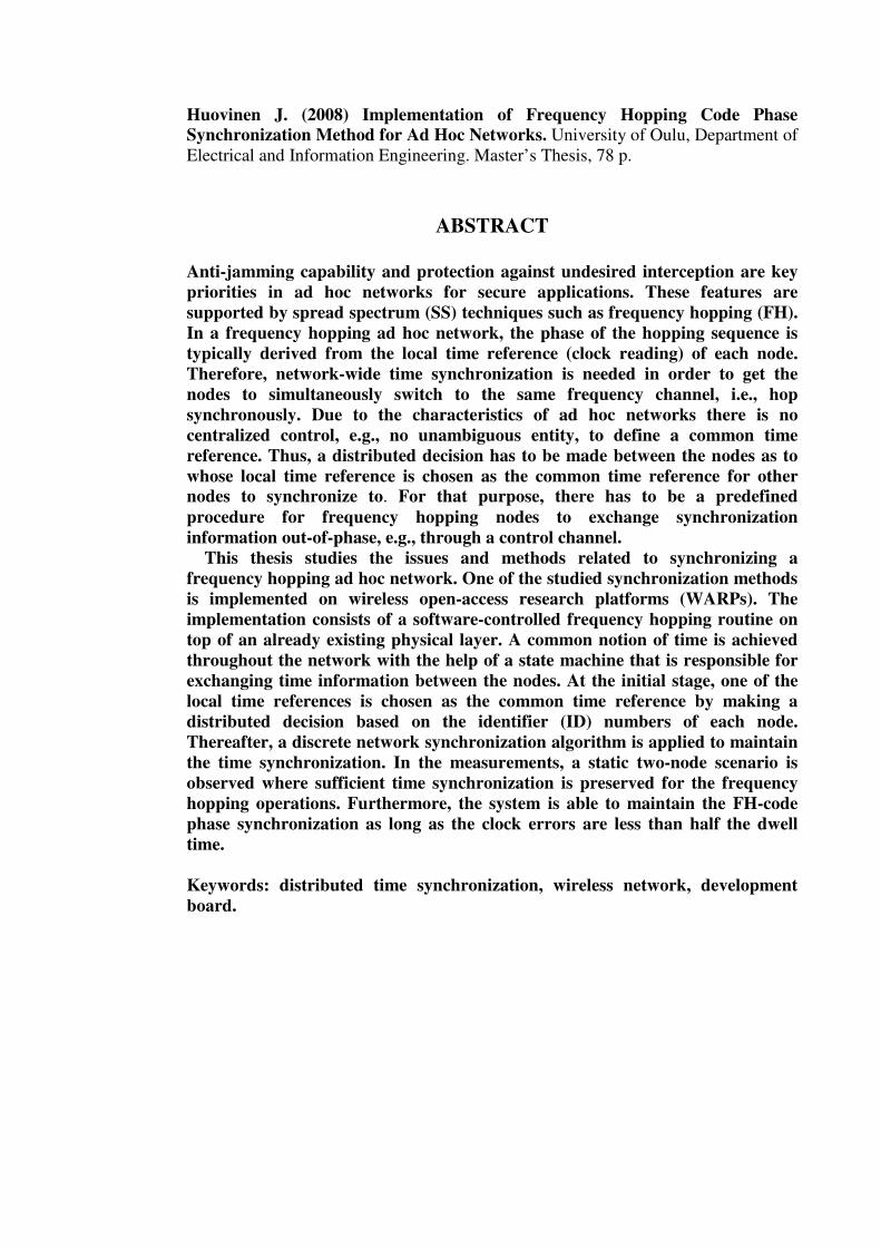
Huovinen J. (2008) Implementation of Frequency Hopping Code Phase Synchronization Method for Ad Hoc Networks. University of Oulu, Department of Electrical and Information Engineering. Master’s Thesis, 78 p.

ABSTRACT

Anti-jamming capability and protection against undesired interception are key priorities in ad hoc networks for secure applications. These features are supported by spread spectrum (SS) techniques such as frequency hopping (FH). In a frequency hopping ad hoc network, the phase of the hopping sequence is typically derived from the local time reference (clock reading) of each node. Therefore, network-wide time synchronization is needed in order to get the nodes to simultaneously switch to the same frequency channel, i.e., hop synchronously. Due to the characteristics of ad hoc networks there is no centralized control, e.g., no unambiguous entity, to define a common time reference. Thus, a distributed decision has to be made between the nodes as to whose local time reference is chosen as the common time reference for other nodes to synchronize to. For that purpose, there has to be a predefined procedure for frequency hopping nodes to exchange synchronization information out-of-phase, e.g., through a control channel. This thesis studies the issues and methods related to synchronizing a frequency hopping ad hoc network. One of the studied synchronization methods is implemented on wireless open-access research platforms (WARPs). The implementation consists of a software-controlled frequency hopping routine on top of an already existing physical layer. A common notion of time is achieved throughout the network with the help of a state machine that is responsible for exchanging time information between the nodes. At the initial stage, one of the local time references is chosen as the common time reference by making a distributed decision based on the identifier (ID) numbers of each node. Thereafter, a discrete network synchronization algorithm is applied to maintain the time synchronization. In the measurements, a static two-node scenario is observed where sufficient time synchronization is preserved for the frequency hopping operations. Furthermore, the system is able to maintain the FH-code phase synchronization as long as the clock errors are less than half the dwell time.

Keywords: distributed time synchronization, wireless network, development board.

Huovinen J. (2008) Taajuushyppykoodivaiheen synkronointimenetelmän toteutus ad hoc -verkoille. Oulun yliopisto, sähkö- ja tietotekniikan osasto. Diplomityö, 78 s.

TIIVISTELMÄ Kyky sietää häirintää ja vaikea salakuunneltavuus ovat etusijalla turvallisuuspainotteisissa rakenteettomien (ad hoc) verkkojen sovelluksissa. Tällaisia ominaisuuksia saavutetaan taajuushyppyhajaspektritekniikkaa hyödyntämällä. Taajuushyppivässä ad hoc -verkossa hyppysekvenssin vaihe on tyypillisesti johdettu suoraan verkon solmujen paikallisesta aikareferenssistä (kellolukemasta). Tällöin tarvitaan verkonlaajuista aikasynkronointia, jotta solmut vaihtaisivat samanaikaisesti samalle taajuuskanavalle eli hyppisivät synkronisesti. Ominaispiirteidensä takia verkolla ei ole keskitettyä kontrollia, joten puuttuu myös yksiselitteinen taho, joka määrittelisi yleisen aikareferenssin. Tämän takia alkutilanteessa on tehtävä hajautettu päätös siitä, minkä solmun paikallinen kellolukema valitaan yhteiseksi aikareferenssiksi verkon kaikille solmuille. Tätä varten tarvitaan ennalta määritelty menettelytapa synkronointi-informaation välittämiseen eri hyppykoodin vaiheessa olevien solmujen kesken. Tämä diplomityö tarkastelee ongelmia ja menetelmiä, jotka liittyvät taajuushyppivän ad hoc -verkon synkronointiin. Yksi menetelmistä toteutetaan langattomille kehitysalustoille (wireless open-access research platform, WARP). Toteutus koostuu ohjelmistokontrolloidusta taajuushyppyrutiinista, joka sijaitsee valmiin fyysisen kerroksen yläpuolella. Aikainformaation välittämiseen solmujen kesken on toteutettu tilakone, jonka avulla saavutetaan koko verkon kattava yhteinen käsitys ajasta. Alkutilanteessa yksi paikallisista kellolukemista valitaan yleiseksi aikareferenssiksi käyttäen hierarkiaa, joka pohjautuu solmujen tunnistenumeroon. Tämän jälkeen käytetään diskreettiä verkon synkronointialgoritmia ylläpitämään ajastus. Mittauksissa tarkastellaan kahden solmun staattista skenaariota, jossa saavutetaan riittävä ajastus taajuushyppytoiminnoille. Lisäksi järjestelmä kykenee ylläpitämään hyppykoodin vaiheen synkronoituna niin kauan kuin kellovirheet ovat alle puolet taajuushypyn kestosta.

Avainsanat: hajautettu aikasynkronointi, langaton verkko, kehitysalusta.

TABLE OF CONTENTS ABSTRACT TIIVISTELMÄ TABLE OF CONTENTS PREFACE LIST OF SYMBOLS AND ABBREVIATIONS 1. INTRODUCTION ..................................................................................................10 2. WIRELESS AD HOC NETWORKS .....................................................................12

2.1. Characteristics..................................................................................................12 2.2. Medium access control ....................................................................................13

2.2.1. Carrier sense multiple access.................................................................14 2.2.2. Code division multiple access ...............................................................15 2.2.3. Bi-code channel access ..........................................................................17

2.3. Routing.............................................................................................................18 2.3.1. Conventional protocols..........................................................................18 2.3.2. Protocols for ad hoc networks ...............................................................19

3. TIME SYNCHRONIZATION................................................................................21 3.1. Classifications ..................................................................................................21 3.2. Clock inaccuracies ...........................................................................................22 3.3. Requirements in ad hoc networks ....................................................................23 3.4. Synchronization protocols ...............................................................................24

3.4.1. Reference-broadcast synchronization....................................................25 3.4.2. Römer’s synchronization algorithm ......................................................25 3.4.3. Lightweight tree-based synchronization................................................26 3.4.4. Discrete network synchronization algorithm.........................................26

4. FREQUENCY HOPPING ......................................................................................28 4.1. Advantages.......................................................................................................29 4.2. Synchronously hopping ad hoc network..........................................................30 4.3. Code phase synchronization methods..............................................................31

5. SYNCHRONIZATION METHOD ........................................................................33 5.1. Control channel in code-space .........................................................................33 5.2. Method description ..........................................................................................34

5.2.1. Transmitting the signal ..........................................................................34 5.2.2. Receiving the signal...............................................................................35 5.2.3. Synchronization message ......................................................................37 5.2.4. Node hierarchy ......................................................................................38

6. METHOD IMPLEMENTATION...........................................................................39 6.1. Wireless open-access research platform ..........................................................39

6.1.1. Board architecture..................................................................................40 6.1.2. Embedded PowerPC..............................................................................41 6.1.3. Reference design....................................................................................43

6.2. System design ..................................................................................................45 6.2.1. Implementation requirements ................................................................46 6.2.2. Medium access control process .............................................................46 6.2.3. Synchronization process ........................................................................48 6.2.4. Software clock .......................................................................................51 6.2.5. Event scheduling....................................................................................52 6.2.6. Time synchronization algorithm............................................................53

6.2.7. Frequency hopping functionality...........................................................54 6.2.8. Control channel functionality ................................................................57

7. DEMONSTRATION CASES.................................................................................59 7.1. Spectrum and time-domain analysis ................................................................59 7.2. Signal-to-noise ratio requirement ....................................................................61 7.3. Clock drift rate .................................................................................................62 7.4. Synchronization message interval....................................................................62 7.5. Effects of increased hopping rate.....................................................................63 7.6. Recovery from initial clock error.....................................................................66

8. DISCUSSION.........................................................................................................67 9. SUMMARY............................................................................................................70 10. REFERENCES .....................................................................................................72 11. APPENDIXES ......................................................................................................77

PREFACE The work in this thesis was carried out at the Centre for Wireless Communications (CWC), University of Oulu. The work is a part of security and defence (S&D) research in the area of wireless ad hoc and sensor networks. The purpose of this thesis was to study the issues and methods related to synchronizing a frequency hopping ad hoc network and demonstrate one of the studied synchronization methods through an implementation on research platforms. I would like to thank my thesis supervisor Professor Jari Iinatti for the comments and suggestions during the regular meetings, my thesis instructor M. Sc. Teemu Vanninen for his guidance and advice throughout this work, and Dr. Tech. Harri Saarnisaari for reviewing my thesis. I would also like to thank the WARP team at Rice University for help with the boards. Finally, thanks go to my parents for their continuous support and encouragement. Oulu, 14 May 2008. Juha Huovinen

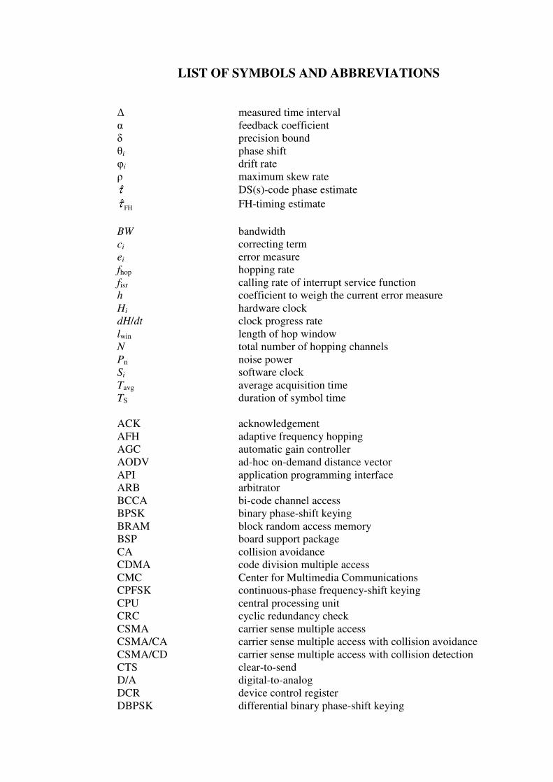
LIST OF SYMBOLS AND ABBREVIATIONS ∆ measured time interval α feedback coefficient δ precision bound θi phase shift φi drift rate ρ maximum skew rate τ̂ DS(s)-code phase estimate

FHτ̂ FH-timing estimate

BW bandwidth ci correcting term

ei error measure

fhop hopping rate

fisr calling rate of interrupt service function h coefficient to weigh the current error measure Hi hardware clock dH/dt clock progress rate lwin length of hop window N total number of hopping channels

Pn noise power Si software clock Tavg average acquisition time

TS duration of symbol time ACK acknowledgement AFH adaptive frequency hopping AGC automatic gain controller AODV ad-hoc on-demand distance vector API application programming interface ARB arbitrator BCCA bi-code channel access BPSK binary phase-shift keying BRAM block random access memory BSP board support package CA collision avoidance CDMA code division multiple access CMC Center for Multimedia Communications CPFSK continuous-phase frequency-shift keying CPU central processing unit CRC cyclic redundancy check CSMA carrier sense multiple access CSMA/CA carrier sense multiple access with collision avoidance CSMA/CD carrier sense multiple access with collision detection CTS clear-to-send D/A digital-to-analog DCR device control register DBPSK differential binary phase-shift keying

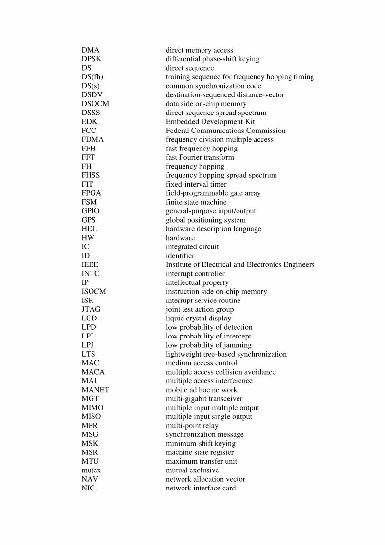
DMA direct memory access DPSK differential phase-shift keying DS direct sequence DS(fh) training sequence for frequency hopping timing DS(s) common synchronization code DSDV destination-sequenced distance-vector DSOCM data side on-chip memory DSSS direct sequence spread spectrum EDK Embedded Development Kit FCC Federal Communications Commission FDMA frequency division multiple access FFH fast frequency hopping FFT fast Fourier transform FH frequency hopping FHSS frequency hopping spread spectrum FIT fixed-interval timer FPGA field-programmable gate array FSM finite state machine GPIO general-purpose input/output GPS global positioning system HDL hardware description language HW hardware IC integrated circuit ID identifier IEEE Institute of Electrical and Electronics Engineers INTC interrupt controller IP intellectual property ISOCM instruction side on-chip memory ISR interrupt service routine JTAG joint test action group LCD liquid crystal display LPD low probability of detection LPI low probability of intercept LPJ low probability of jamming LTS lightweight tree-based synchronization MAC medium access control MACA multiple access collision avoidance MAI multiple access interference MANET mobile ad hoc network MGT multi-gigabit transceiver MIMO multiple input multiple output MISO multiple input single output MPR multi-point relay MSG synchronization message MSK minimum-shift keying MSR machine state register MTU maximum transfer unit mutex mutual exclusive NAV network allocation vector NIC network interface card

NTP network time protocol NWID network identifier OCM on-chip memory OFDM orthogonal frequency-division multiplexing OFDMA orthogonal frequency division multiple access OLSR optimized link state routing OPB on-chip peripheral bus OS operating system OSI open system interconnection PDI post detection integration PG processing gain PIT programmable-interval timer PHY physical layer PLB processor local bus PLL phase-locked loop PLR packet loss ratio PN pseudo-noise PPC PowerPC ppm parts per million PSD power spectral density PRNG pseudo-random number generator QAM quadrature amplitude modulation QoS quality of service RBS reference-broadcast synchronization RREP route reply RREQ route request RSSI received signal strength indicator RTOS real-time operating system RTS request-to-send RX reception SFH slow frequency hopping SNR signal-to-noise ratio SRAM static random access memory SS spread spectrum SRR save/restore register SW software SWAP-CA shared wireless access protocol-cordless access TDMA time division multiple access TH time hopping TX transmission UART universal asynchronous receiver/transmitter USB universal serial bus UTC coordinated universal time WARP wireless open-access research platform WDT watchdog timer WLAN wireless local area network WSN wireless sensor network XBD Xilinx board description XPS Xilinx Platform Studio

1. INTRODUCTION There are various applications for ad hoc networks in circumstances where a wireless network is required for nodes to directly communicate with each other without an intermediate base station. One of the application areas is the military field where security and robustness against, e.g., jamming and interception are key requirements in the design of a network. Such properties potentially exist in systems utilizing spread spectrum (SS) techniques such as frequency hopping (FH). These signals have a low average power spectral density (PSD) due to spreading the original narrowband transmission over a wider spectrum, which makes the signals more difficult to detect from the background noise by outside users. In a frequency hopping ad hoc network, it is usually a fair assumption that the nodes know the hopping sequence in advance. A hopping sequence, also called an FH-code, consists of a set of available channels arranged in a pseudo-random order. Provided that a long enough pseudo-random FH-code is used, unintended users are not able to determine the hopping pattern and use that information to intercept the transmission. Once a network is formed, the nodes are using the hopping sequence to operate on a channel that it is currently pointing to. After a certain time period depending on the hopping rate, the current channel is switched to the next one in this predefined hopping sequence. To be able to join the network, a node must determine at which point in the code the other nodes are currently hopping, i.e., it must synchronize to the FH-code phase of the network. Typically, the FH-code phase is directly derived from the local clock reading of a node. In that case, network-wide time synchronization plays an important role in acquiring and maintaining the FH-code phase throughout the network. For example, in a start-up scenario the nodes are likely to have different local clock readings such that each node accordingly operates with a different phase offset of the same hopping sequence. Since there is no centralized control in ad hoc networks, synchronizing a frequency hopping waveform can be problematic because no common time reference is available. For this reason, there has to be a predefined acquisition procedure that allows nodes to exchange synchronization information even if they are operating out-of-phase against each other. Once the synchronization information has been exchanged, a distributed decision must be made as to whose local clock reading is chosen as the common time reference for the other nodes to synchronize to. Thereafter, a time synchronization algorithm should be applied in order to maintain the synchronization throughout the network because the local clocks of nodes tend to drift due to frequency deviations of oscillators. In this thesis, different methods to acquire and maintain FH-code phase synchronization are reviewed. One of the reviewed synchronization methods is chosen to be implemented on research platforms that allow wireless communication over the air. A reference design functions as a starting point for the work, and it is further modified according to the needs of the synchronization method and enhanced with frequency hopping capability. Lastly, the implementation is verified to be consistent with the design and a number of test cases are run for both the FH-code phase synchronization method and the frequency hopping functionality. This thesis is organized as follows. In Chapter 2, there is an overview of the characteristics of wireless ad hoc networks including the particular issues in medium access control and routing protocols. Chapter 3 deals with the problem of clock inaccuracies and time synchronization specifically from the perspective of ad hoc networks. In

11

addition, a number of protocols for time synchronization are presented to give concrete examples of the outlined properties. In Chapter 4, the principles and advantages of frequency hopping spread spectrum (FHSS) systems are discussed and how FHSS is used in multiple access scenarios or synchronously hopping ad hoc networks where all the nodes have a common hopping sequence. Additionally, several FH-code phase synchronization methods are studied. Chapter 5 thoroughly describes one of these methods from the transmission to the reception of the signal. The implementation of this chosen method is documented in Chapter 6, which first presents the research platforms and the reference design, and continues to a detailed description of the system design. In Chapter 7, a series of verification tests and demonstration cases are run, which are then discussed in Chapter 8 in addition to the further development ideas of the current implementation. Finally, the work is summarized in Chapter 9.

12

2. WIRELESS AD HOC NETWORKS An ad hoc network is a collection of devices that communicate with each other without any fixed infrastructure or the help of centralized control. The nodes, which are usually wireless and mobile, may join and leave networks while moving around arbitrarily. Therefore, these mobile ad hoc networks (MANETs) are formed only temporarily, and the nodes have the ability to quickly adapt to a continuously changing network topology. The highly adaptive structure of ad hoc networks enables plenty of different applications. For instance, there might be situations when conventional infrastructure is damaged or non-existent. Ad hoc networks are fast to set up and do not lose functionality if some of the nodes are non-operable. One of the most interesting applications is a network of sensor-equipped nodes, a wireless sensor network (WSN), which is suitable for various measuring, monitoring and surveillance purposes [1]. In this chapter, there is a brief overview of wireless ad hoc networks including characteristics, medium access control and routing.

2.1. Characteristics Since there is no centralized administration, ad hoc networks must be organized in a distributed fashion. The nodes can discover neighbors, determine how to route data and synchronize with each other by using distributed algorithms and protocols [2 p. 67]. The term self-organization is commonly used. The purpose of self-organization is to ensure the scalability, reliability and availability of networks that may consist of a huge number of individual nodes [3]. Scalability describes whether the performance of a network stays the same when adding more and more nodes to the network. This is an important factor especially in wireless sensor networks, which might have thousands or even hundreds of thousands of sensor nodes deployed in one area [1]. The possibility of extremely variable network size and density should be kept in mind during the design process of protocols and algorithms. Even if a number of nodes run out of energy, or a group of nodes decide to leave the network making the topology to change dramatically, the functionality of the network should be assured by finding other routes for broken radio links and compensating for all other failures [2 p. 67]. This is often referred to as self-configuring property in the literature. In ad hoc networks, it is crucial to conserve limited resources such as network capacity and battery power. Energy consumption can be minimized by using different power saving techniques that turn off components of devices not in use, and perhaps, control the available transmission and reception power. There might be long periods of little or no activity in the network in which case redundantly operating radios, for example, would be a huge waste of energy. [4] Different topology control methods can be used to optimize energy usage and network lifetime [5]. Besides changing the transmission powers of nodes, the links between the nodes can be arranged and controlled to get the desired topology. Some of the links can be temporarily discarded and unnecessary nodes can be switched off completely. In a hierarchical network topology, some nodes have special roles. For example, a group of nodes can function as a backbone to which all other nodes are directing their links, or the topology can be partitioned into clusters when only the links within a cluster are maintained as well as some selected links between clusters

13

to ensure connectivity of the whole network [2 p. 252]. In these cases, the system may be more vulnerable to attacks because wiping out the nodes at the top of the hierarchy might incapacitate the whole system. Hence, robustness should be assured especially in military applications, so that the system is able to recover even if these prime nodes get destroyed. Additionally, the topology control methods have abilities to increase the performance of the network and decrease end-to-end delays. Instead of establishing connections with all the neighboring nodes within the transmission range of a node, it is more desirable to choose only those local connections that will guarantee overall global network connectivity while satisfying different performance metrics such as overall throughput, network utilization, and power dissipation [6].

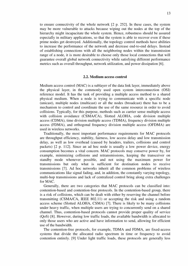
2.2. Medium access control Medium access control (MAC) is a sublayer of the data link layer, immediately above the physical layer, in the commonly used open system interconnection (OSI) reference model. It has the task of providing a multiple access method to a shared physical medium. When a node is trying to communicate with a specific node (unicast), multiple nodes (multicast) or all the nodes (broadcast) there has to be a mechanism to control and coordinate the use of the same resource in order to avoid collisions. Typically, for this purpose, methods such as carrier sense multiple access with collision avoidance (CSMA/CA), Slotted ALOHA, code division multiple access (CDMA), time division multiple access (TDMA), frequency division multiple access (FDMA), and orthogonal frequency division multiple access (OFDMA) are used in wireless networks. Traditionally, the most important performance requirements for MAC protocols are throughput efficiency, stability, fairness, low access delay and low transmission delay, as well as low overhead (caused by headers, trailers, collisions and control packets) [2 p. 112]. Since an ad hoc node is usually a low power device, energy consumption becomes a vital concern. MAC protocols may conserve power by, for example, minimizing collisions and retransmissions, keeping the transceiver on standby mode whenever possible, and not using the maximum power for transmissions but only what is sufficient for destination nodes to receive transmissions [7]. Ad hoc networks inherit all the common problems of wireless communications like signal fading, and, in addition, the constantly varying topology, multi-hop transmissions and lack of centralized control bring along extra challenges for MAC. Generally, there are two categories that MAC protocols can be classified into: contention-based and contention-free protocols. In the contention-based group, there is a risk of collisions, which can be dealt with either by reserving the channel before transmitting (CSMA/CA, IEEE 802.11) or accepting the risk and using a random access scheme (Slotted ALOHA, CSMA) [7]. There is likely to be many collisions under heavy traffic, when multiple users are trying to concurrently send on a shared channel. Thus, contention-based protocols cannot provide proper quality of service (QoS) [8]. However, during low traffic loads, the available bandwidth is allocated to only those users who are active and have information to send, allowing for efficient use of the bandwidth. The contention-free protocols, for example, TDMA and FDMA, are fixed-access systems that divide the allocated radio spectrum in time or frequency to avoid contention entirely. [9] Under light traffic loads, these protocols are generally less

14

efficient than contention-based protocols, because a certain amount of the channel capacity is typically allocated to each user, most of whom could be in an idle state. For that reason, contention-free protocols are more suitable for steady data flows. [8] There are also multiple channel schemes, hybrids of the above categories, having a common channel for control packets and another channel for data packets to help reduce collisions. Furthermore, classifications can be made considering properties like QoS awareness and power awareness. [7]

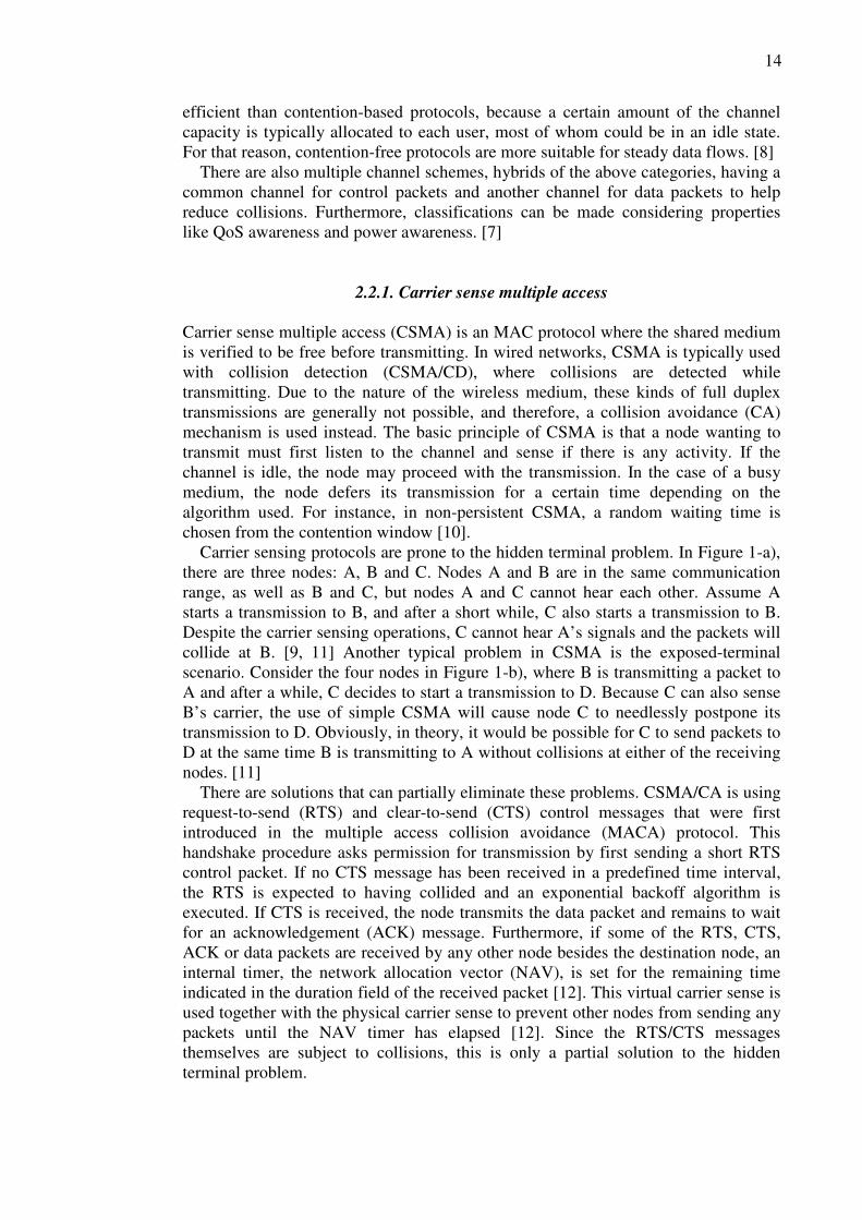
2.2.1. Carrier sense multiple access Carrier sense multiple access (CSMA) is an MAC protocol where the shared medium is verified to be free before transmitting. In wired networks, CSMA is typically used with collision detection (CSMA/CD), where collisions are detected while transmitting. Due to the nature of the wireless medium, these kinds of full duplex transmissions are generally not possible, and therefore, a collision avoidance (CA) mechanism is used instead. The basic principle of CSMA is that a node wanting to transmit must first listen to the channel and sense if there is any activity. If the channel is idle, the node may proceed with the transmission. In the case of a busy medium, the node defers its transmission for a certain time depending on the algorithm used. For instance, in non-persistent CSMA, a random waiting time is chosen from the contention window [10]. Carrier sensing protocols are prone to the hidden terminal problem. In Figure 1-a), there are three nodes: A, B and C. Nodes A and B are in the same communication range, as well as B and C, but nodes A and C cannot hear each other. Assume A starts a transmission to B, and after a short while, C also starts a transmission to B. Despite the carrier sensing operations, C cannot hear A’s signals and the packets will collide at B. [9, 11] Another typical problem in CSMA is the exposed-terminal scenario. Consider the four nodes in Figure 1-b), where B is transmitting a packet to A and after a while, C decides to start a transmission to D. Because C can also sense B’s carrier, the use of simple CSMA will cause node C to needlessly postpone its transmission to D. Obviously, in theory, it would be possible for C to send packets to D at the same time B is transmitting to A without collisions at either of the receiving nodes. [11] There are solutions that can partially eliminate these problems. CSMA/CA is using request-to-send (RTS) and clear-to-send (CTS) control messages that were first introduced in the multiple access collision avoidance (MACA) protocol. This handshake procedure asks permission for transmission by first sending a short RTS control packet. If no CTS message has been received in a predefined time interval, the RTS is expected to having collided and an exponential backoff algorithm is executed. If CTS is received, the node transmits the data packet and remains to wait for an acknowledgement (ACK) message. Furthermore, if some of the RTS, CTS, ACK or data packets are received by any other node besides the destination node, an internal timer, the network allocation vector (NAV), is set for the remaining time indicated in the duration field of the received packet [12]. This virtual carrier sense is used together with the physical carrier sense to prevent other nodes from sending any packets until the NAV timer has elapsed [12]. Since the RTS/CTS messages themselves are subject to collisions, this is only a partial solution to the hidden terminal problem.

15

a) Hidden terminal problem.

b) Exposed terminal problem. Figure 1. CSMA problem scenarios.

2.2.2. Code division multiple access

Code division multiple access (CDMA) is a method that enables the allocated radio spectrum to be used by multiple users simultaneously. Traditionally, the available spectrum is allocated either in frequency or time slots. CDMA does not make this kind of fixed division by frequency or time, but assigns a unique spreading code to each user and utilizes spread spectrum techniques such as frequency hopping, time hopping (TH), and most commonly, direct sequence (DS). A direct sequence spread spectrum (DSSS) system is using pseudo-random or pseudo-noise (PN) sequences to modify the signal. One PN-code symbol is called a chip and it has a much shorter duration than an information bit, as illustrated in Figure 2. The phase of the carrier is modulated pseudo-randomly according to the code pattern from the PN-generator [13 p. 729]. Next, this higher bit rate signal modulates the information bits, and the data get spread over a wider spectrum. As a result, the data occupy a much larger bandwidth than would be necessary, but at the same time, the power spectral density is getting very low, giving the signal noise-like appearance in the channel. The waveforms of the original narrowband signal and the resulting spread spectrum signal are shown in Figure 3-a) and Figure 3-b) respectively.

A

B

C

A

B C D

16

Figure 2. Pseudo-noise spreading.

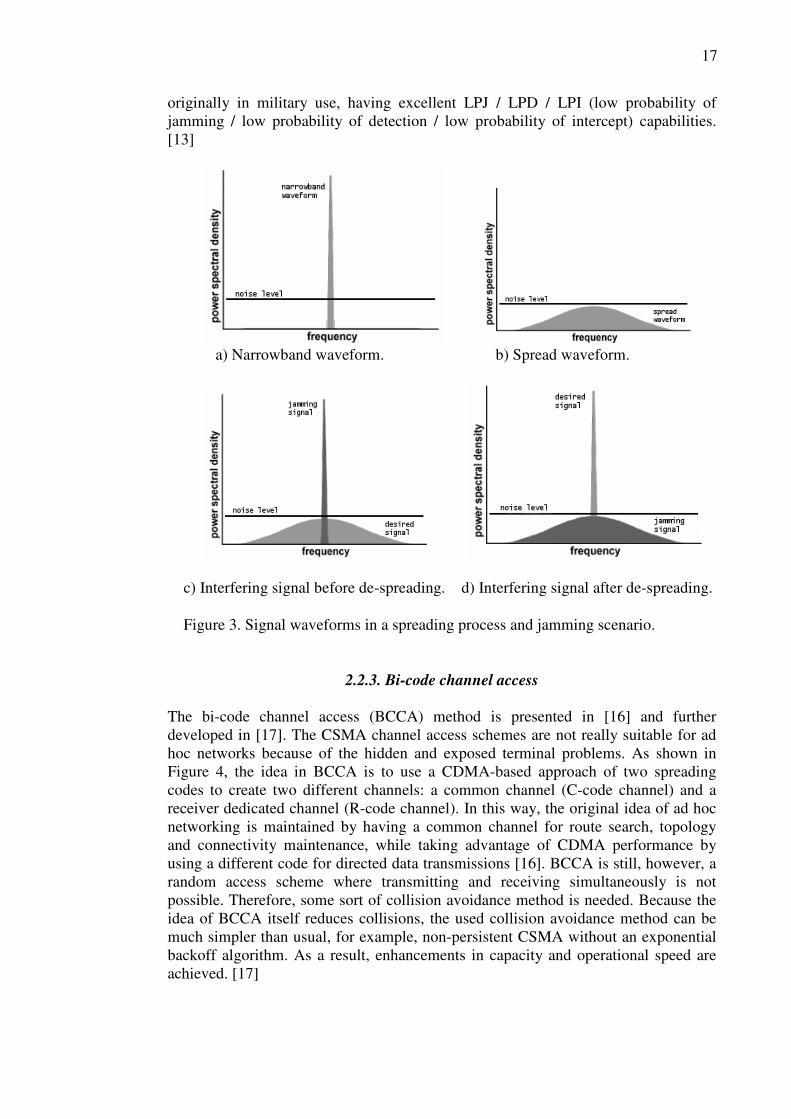
The ratio between the chips and information bits is called the processing gain (PG) or the spreading factor, and along with the energy of the received broadband signal, it must be high enough to provide an adequate signal-to-noise ratio (SNR) at the receiver. The processing gain and other properties of a DS spread system enable multiple signals to occupy the same channel bandwidth at the same time, provided that each signal has a distinct PN-code [13 p. 747]. This is the feature CDMA is exploiting to allow several users to transmit simultaneously. The receiver can distinguish each user with the help of the same PN-code used in the transmission. In order to successfully recover the original data at the receiver, mutually orthogonal spreading codes with good autocorrelation and low cross-correlation properties are preferred. The key factor as to why CDMA has yet to extend comprehensively to ad hoc networks is the so-called near-far problem [14]. Consider a scenario of one receiver node and two transmitter nodes, of which the other one is much farther away from the receiver. If both of the transmitters are trying to transmit at the same time at equal power, the signal from the nearer transmitter will arrive with a much larger power to the receiver. It might not be possible to detect the further signal because the stronger transmission from the nearer node is acting as disturbing noise for the desired signal. This noise, called multiple access interference (MAI), results from nonzero cross-correlation components between different CDMA codes [15]. To overcome the near-far problem, dynamic power control techniques are used so that the transmission power is limited in relation to the distance to the receiver; the closer the transmitter is, the less power it uses [15]. As a result, the receiver attains roughly the same SNR for all transmitters. The requirement for distributed functionality makes the power control techniques difficult to implement in ad hoc networks. Beside the multiple access properties, there are several other advantages in CDMA. The common problem of multipath effects can be mitigated by combining the reflected signals with different time delays to make a stronger signal in a rake receiver [15]. Even though the spreading codes are mainly intended for user identification purposes, they also provide security since it is almost impossible to recover the original data without knowing the spreading code. Additionally, increased resistance to jamming is achieved due to the widely spread bandwidth as illustrated in Figure 3-c) and Figure 3-d), and at the same time, the transmission can be disguised below the noise level, making it hard to detect for any unauthorized parties. These properties of a spread spectrum system are the main reason why CDMA was

17

originally in military use, having excellent LPJ / LPD / LPI (low probability of jamming / low probability of detection / low probability of intercept) capabilities. [13]

a) Narrowband waveform. b) Spread waveform.

c) Interfering signal before de-spreading. d) Interfering signal after de-spreading.

Figure 3. Signal waveforms in a spreading process and jamming scenario.

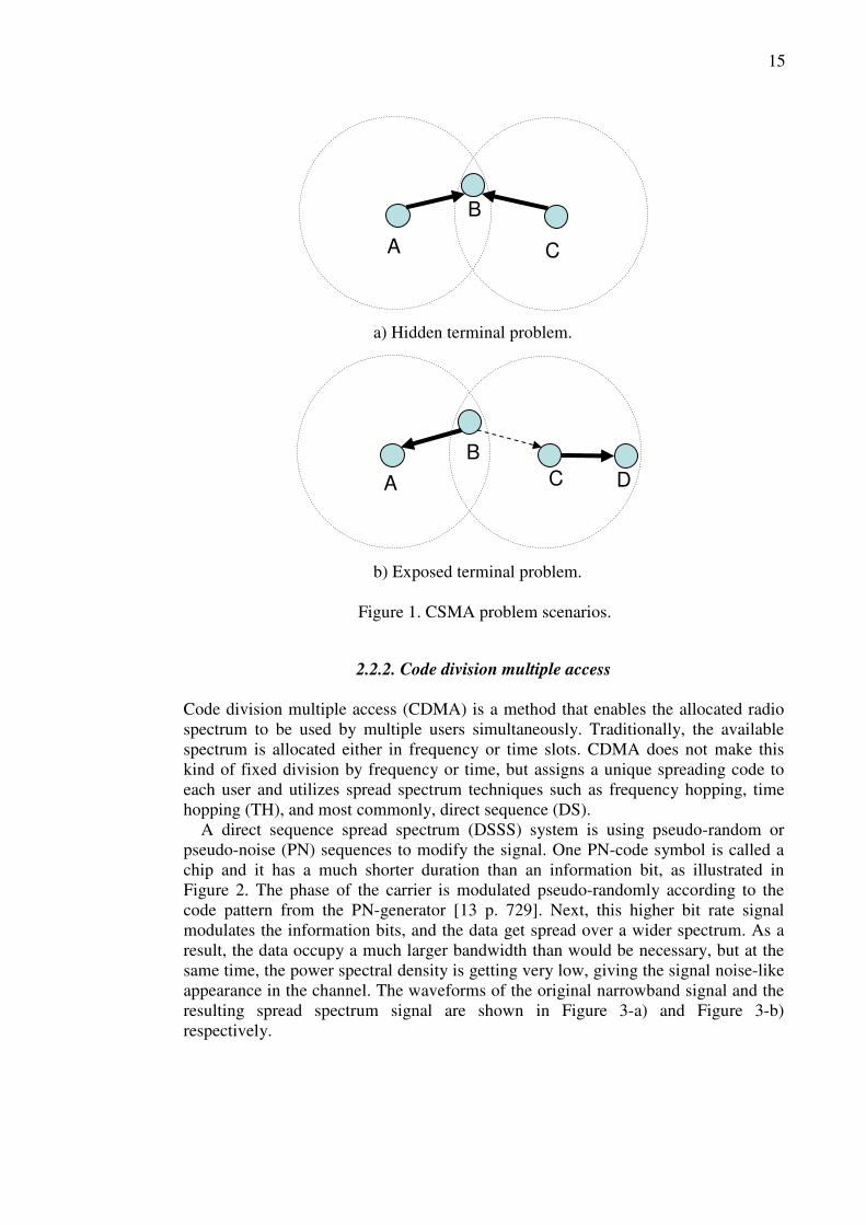
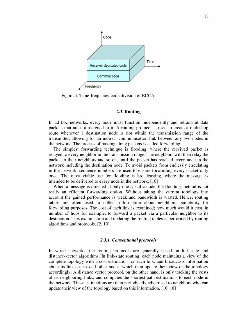
2.2.3. Bi-code channel access The bi-code channel access (BCCA) method is presented in [16] and further developed in [17]. The CSMA channel access schemes are not really suitable for ad hoc networks because of the hidden and exposed terminal problems. As shown in Figure 4, the idea in BCCA is to use a CDMA-based approach of two spreading codes to create two different channels: a common channel (C-code channel) and a receiver dedicated channel (R-code channel). In this way, the original idea of ad hoc networking is maintained by having a common channel for route search, topology and connectivity maintenance, while taking advantage of CDMA performance by using a different code for directed data transmissions [16]. BCCA is still, however, a random access scheme where transmitting and receiving simultaneously is not possible. Therefore, some sort of collision avoidance method is needed. Because the idea of BCCA itself reduces collisions, the used collision avoidance method can be much simpler than usual, for example, non-persistent CSMA without an exponential backoff algorithm. As a result, enhancements in capacity and operational speed are achieved. [17]

18

Figure 4. Time-frequency-code division of BCCA.

2.3. Routing In ad hoc networks, every node must function independently and retransmit data packets that are not assigned to it. A routing protocol is used to create a multi-hop route whenever a destination node is not within the transmission range of the transmitter, allowing for an indirect communication link between any two nodes in the network. The process of passing along packets is called forwarding. The simplest forwarding technique is flooding, where the received packet is relayed to every neighbor in the transmission range. The neighbors will then relay the packet to their neighbors and so on, until the packet has reached every node in the network including the destination node. To avoid packets from endlessly circulating in the network, sequence numbers are used to ensure forwarding every packet only once. The most viable use for flooding is broadcasting, where the message is intended to be delivered to every node in the network. [10] When a message is directed at only one specific node, the flooding method is not really an efficient forwarding option. Without taking the current topology into account the gained performance is weak and bandwidth is wasted. Hence, routing tables are often used to collect information about neighbors’ suitability for forwarding purposes. The cost of each link is examined; how much would it cost, in number of hops for example, to forward a packet via a particular neighbor to its destination. This examination and updating the routing tables is performed by routing algorithms and protocols. [2, 10]

2.3.1. Conventional protocols In wired networks, the routing protocols are generally based on link-state and distance-vector algorithms. In link-state routing, each node maintains a view of the complete topology with a cost estimation for each link, and broadcasts information about its link costs to all other nodes, which then update their view of the topology accordingly. A distance vector protocol, on the other hand, is only tracking the costs of its neighboring links, and computes the shortest path estimations to each node in the network. These estimations are then periodically advertised to neighbors who can update their view of the topology based on this information. [10, 18]

19

The problem with using conventional routing protocols in a mobile ad hoc environment is that they were designed for a static topology, and they assume bi-directional links, which is not always the case in wireless systems because the transmission between two hosts may not work equally well in both directions. Even in a static ad hoc network scenario, problems would be encountered due to the periodic need for exchanging control messages. Ad hoc networks may consist of a very large number of nodes, and both link-state and distance-vector algorithms maintain distances to every reachable node in the network. Consequently, this is costly in resources such as bandwidth, battery power and central processing unit (CPU) and is not suitable for MANETs. [19]

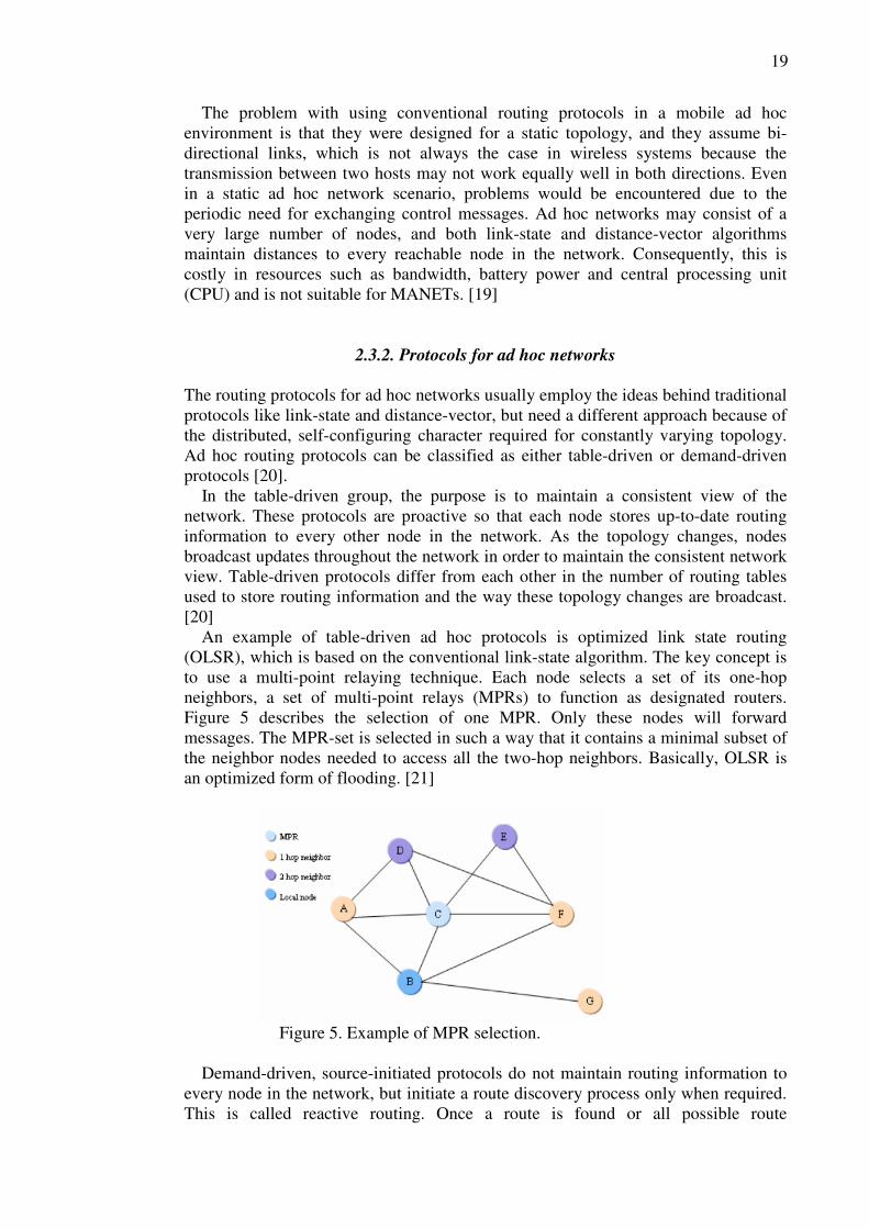
2.3.2. Protocols for ad hoc networks The routing protocols for ad hoc networks usually employ the ideas behind traditional protocols like link-state and distance-vector, but need a different approach because of the distributed, self-configuring character required for constantly varying topology. Ad hoc routing protocols can be classified as either table-driven or demand-driven protocols [20]. In the table-driven group, the purpose is to maintain a consistent view of the network. These protocols are proactive so that each node stores up-to-date routing information to every other node in the network. As the topology changes, nodes broadcast updates throughout the network in order to maintain the consistent network view. Table-driven protocols differ from each other in the number of routing tables used to store routing information and the way these topology changes are broadcast. [20] An example of table-driven ad hoc protocols is optimized link state routing (OLSR), which is based on the conventional link-state algorithm. The key concept is to use a multi-point relaying technique. Each node selects a set of its one-hop neighbors, a set of multi-point relays (MPRs) to function as designated routers. Figure 5 describes the selection of one MPR. Only these nodes will forward messages. The MPR-set is selected in such a way that it contains a minimal subset of the neighbor nodes needed to access all the two-hop neighbors. Basically, OLSR is an optimized form of flooding. [21]

Figure 5. Example of MPR selection. Demand-driven, source-initiated protocols do not maintain routing information to every node in the network, but initiate a route discovery process only when required. This is called reactive routing. Once a route is found or all possible route

20

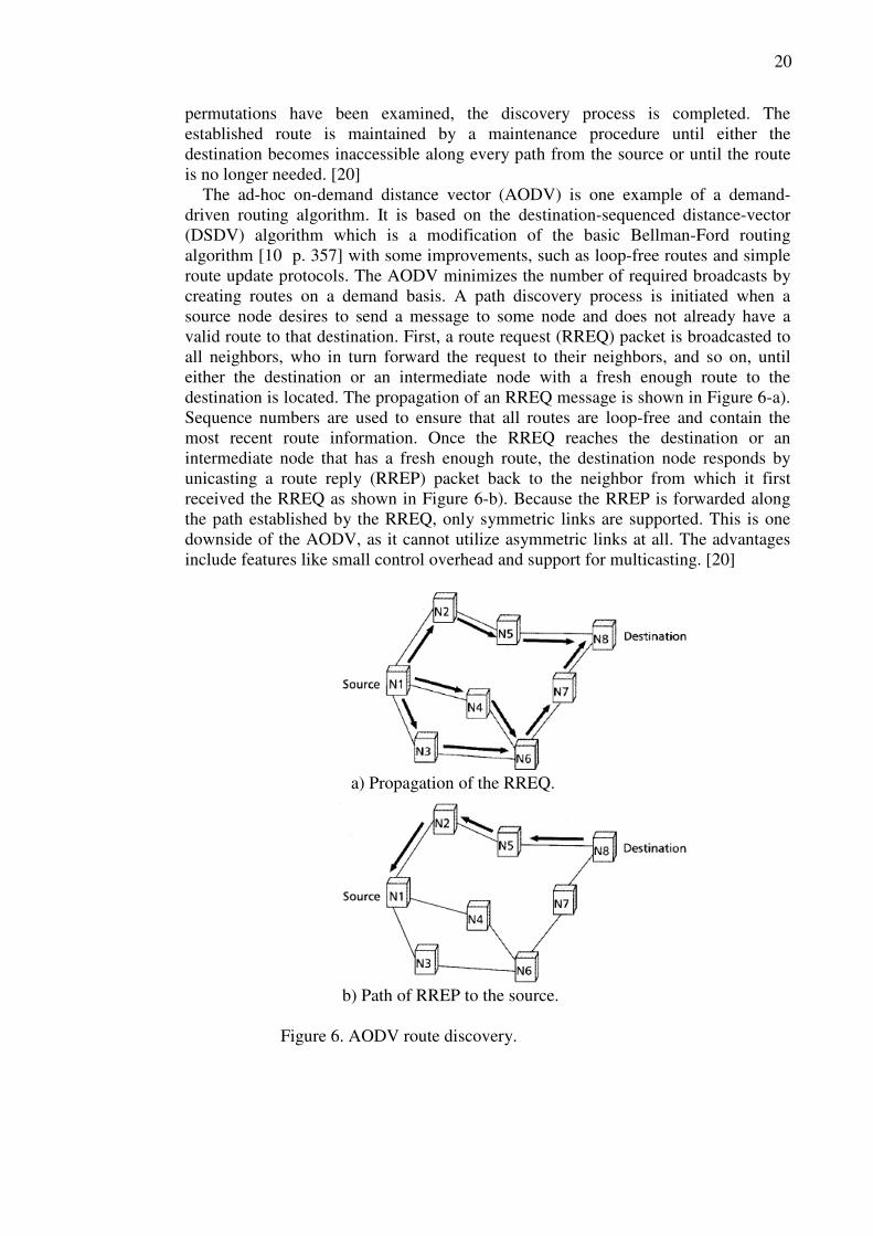
permutations have been examined, the discovery process is completed. The established route is maintained by a maintenance procedure until either the destination becomes inaccessible along every path from the source or until the route is no longer needed. [20] The ad-hoc on-demand distance vector (AODV) is one example of a demand-driven routing algorithm. It is based on the destination-sequenced distance-vector (DSDV) algorithm which is a modification of the basic Bellman-Ford routing algorithm [10 p. 357] with some improvements, such as loop-free routes and simple route update protocols. The AODV minimizes the number of required broadcasts by creating routes on a demand basis. A path discovery process is initiated when a source node desires to send a message to some node and does not already have a valid route to that destination. First, a route request (RREQ) packet is broadcasted to all neighbors, who in turn forward the request to their neighbors, and so on, until either the destination or an intermediate node with a fresh enough route to the destination is located. The propagation of an RREQ message is shown in Figure 6-a). Sequence numbers are used to ensure that all routes are loop-free and contain the most recent route information. Once the RREQ reaches the destination or an intermediate node that has a fresh enough route, the destination node responds by unicasting a route reply (RREP) packet back to the neighbor from which it first received the RREQ as shown in Figure 6-b). Because the RREP is forwarded along the path established by the RREQ, only symmetric links are supported. This is one downside of the AODV, as it cannot utilize asymmetric links at all. The advantages include features like small control overhead and support for multicasting. [20]

a) Propagation of the RREQ.

b) Path of RREP to the source.

Figure 6. AODV route discovery.

21

3. TIME SYNCHRONIZATION There are numerous applications and protocols that are dependent on the internal clock of a node. To measure time, each node has a local clock that is driven by an oscillator. Due to the random phase shifts of these oscillators, the local clock readings of different nodes are slightly drifting from each other. A synchronization procedure is needed to correct these small differences in clock readings, and accordingly, to keep the hosts synchronized. Time synchronization may play important role in ad hoc networks. For example, in wireless sensor networks, the basic operation is data fusion, in which data from multiple sensors is combined to form a single meaningful result. Because the individual nodes are exchanging sensed information in data packets that are timestamped by their local clocks, a common notion of time is needed to get accurate results from the data fusion. [22] Furthermore, the systems may be using techniques like FHSS or TDMA, where it is essential to have a common notion of time. Such a notion can be accomplished by using clock synchronization protocols.

3.1. Classifications Traditionally, the synchronization protocols are using master-slave or peer-to-peer structures. Master-slave protocols assign one node as the master and all other nodes as slaves. The biggest disadvantage of the master-slave structure is that if the master node fails it affects the whole network. Peer-to-peer is a more robust structure in this sense. Any node can directly synchronize with every other node in the network, and therefore the risk of master node failure is eliminated. Although peer-to-peer methods offer more flexibility, they are more difficult to control. [22, 27] Depending on the time reference, the synchronization method of a network can be either external or internal. In external synchronization, the network uses an external standard like the global positioning system (GPS) or coordinated universal time (UTC) to synchronize to an accurate time source. The internal synchronization, on the other hand, has a floating time within the network and does not have any global time base (real-time) available. The goal is simply to minimize the difference between the readings of local clocks and have consistency among the network nodes. [22, 25] As in reactive routing, there are clock synchronization protocols that perform synchronization on demand, only when it is needed. Such methods are called post-facto synchronization protocols. Energy is conserved by synchronizing the nodes only when it is necessary. At all other times, the nodes can be switched to a power-saving mode. The alternative to a post-facto scheme is a-priori synchronization, where the synchronization messages are continually exchanged in a proactive way. However, in ad hoc networks, the energy constraints may rule out the possibility for a-priori synchronization between arbitrary nodes. [22, 25] There are two ways of achieving a common notion of time. The most often used method is to correct the local clocks of each node to run in sync with the reference time. Either reactive or proactive synchronization methods are used. Another way is to use untethered clocks, where the common notion of time is achieved without synchronization. This is becoming a popular method due to the gained energy savings. [22] Römer’s algorithm [23], for example, determines lower and upper

22

bounds for the real-time passed from the generation of the timestamp at the source node to the arrival of the message at the destination node, and with the help of this interval, the received timestamp is transformed to the local time of the receiver. Römer’s algorithm will be discussed in more detail later in this chapter.

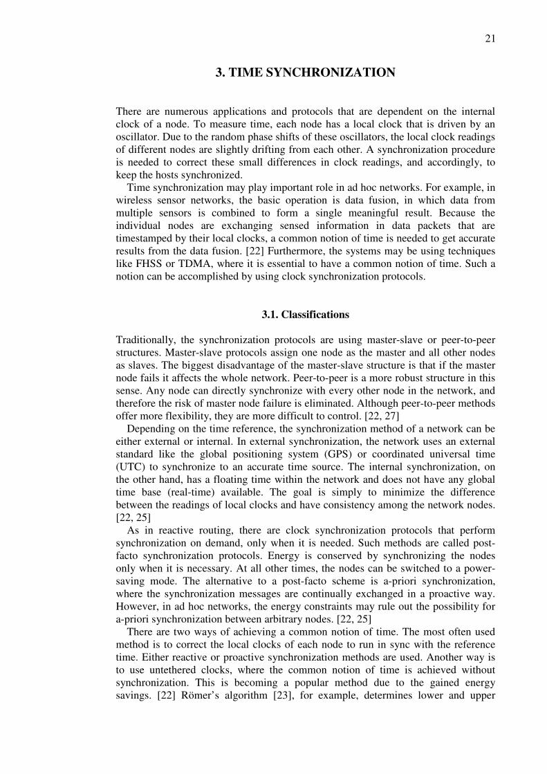
3.2. Clock inaccuracies Contrary to centralized systems, where a process gets the time by simply issuing a system call to the kernel, there is no global clock available in ad hoc networks due to their distributed nature. Each node has its own local clock, and these clocks can easily drift seconds per day, meaning that the common notion of time is eventually lost even if the nodes were synchronized at the start-up. [22] Generally, computer clocks consist of a crystal oscillator and a counter register that is counting the oscillations of the crystal at a particular frequency. A frequency deviation of just 0.001% would cause a clock error of almost one second per day. That is also the reason why clock performance is often measured with very fine units like parts per million (ppm)1. The value for the hardware clock of a node i at real time t can be represented as Hi (t) in which case the clock progresses at a rate of dH/dt. A perfect hardware clock of node i would have Hi (t) = t for all i and t, and thus dH/dt

equals 1. However, this is rarely the case with cheap oscillators used in ad hoc network applications, and therefore the clocks may run faster (dH/dt > 1) or slower (dH/dt < 1) than the perfect clock, as shown in Figure 7. [22]

Figure 7. Fast, slow and perfect clocks with respect to real time. Basically, all hardware clocks are imperfect and subject to clock drift. One can usually assume that the clock drift of a computer clock does not exceed a maximum value of ρ. This can be presented as

ρ1ρ1 +≤≤−dt

dH, (1)

where the constant ρ is also referred to as the maximum skew rate [23]. The frequency of clocks varies over time and is mostly influenced by temperature, air pressure or magnetic fields. Even some of the best clocks available still have errors of

1 Part per million is 10-6. A clock with a drift of 100 ppm drifts 100 seconds in a million seconds [25].

Fast clock dH/dt > 1

Perfect clock dH/dt = 1

Slow clock dH/dt < 1

Real time, t

Har

dwar

e cl

ock,

H

23

about 10-8 ppm [24]. The skew rates for WSNs for example, are typically between 10 - 100 ppm since the sensor nodes usually contain non-expensive oscillators [25]. A clock synchronization algorithm has to be carried out in order to guarantee a certain precision, so that the clock readings of any two non-faulty clocks are within a given bound δ [25]

δ)()( <− tHtH ji , for all { }nji ,...,2,1, ∈ . (2)

In addition, externally synchronized networks aim to guarantee that the difference between any clock of the system and the real time t is [25]

δ)( <− ttH i , for all { }ni ,...,2,1∈ . (3)

The hardware clock Hi (t) can be considered as an abstraction of the counter register that is counting the oscillation pulses. Typically, the local software clock Si (t) is calculated as [2]

iiii tHtS φ )( · θ)( += , (4)

where θi is called the phase shift and φi is called the drift rate. Because it is usually not possible or desirable to modify the frequency of the local node oscillator, one can use a software clock instead and simply change the coefficients θi and φi to do the clock adjustment [2].

3.3. Requirements in ad hoc networks The traditional synchronization schemes for wired networks, such as the network time protocol (NTP), were designed for large-scale networks with a relatively static topology [25]. In a WSN for instance, the energy and other resources are very limited. To synchronize its master nodes, NTP is using technologies like GPS, which could be against the energy constraints in a WSN. Besides, GPS might not be available, e.g., in hostile regions or inside buildings because a clear line-of-sight to the satellites is needed. Since energy-efficiency is not an issue in infrastructure-based distributed systems, it is not considered in any way in the NTP algorithm [25]. NTP proactively synchronizes all the nodes with maximum precision even though only a subset of nodes might occasionally need synchronized time with less than maximum precision [25]. In addition, it maintains synchronism by constantly adjusting the system clock counter, which precludes the processor from being switched to a power-saving mode [26]. NTP also makes no effort to predict the time at which packets will arrive, but simply listens to the network all the time [26]. Most of the traditional synchronization methods assume a fully-connected or low-latency topology, where any node can send a message directly to another node at any point in time in a single-hop fashion. This means there is a constant latency and jitter bound for all messages in the system, and a close approximation for the actual latency can be provided. [26] In a MANET, the topology might be very large, in which case the messages must be transmitted in multiple hops and, additionally, scalability becomes a major concern. Transmitting over multiple short distances instead of a single long path can also be a way to conserve energy [22]. Due to the frequently changing topology and multi-hop transmissions, the end-to-end delays of

24

the message paths are very unstable and hard to predict in ad hoc networks, and thus protocols assuming a fully-connected single-hop network cannot be applied [25]. There are several layers of servers that provide an accurate source of time in NTP [22]. Nodes can find a source of reference time just a few hops away. In MANETs, however, this kind of external infrastructure of time-reference sources is not feasible because of the constantly changing topology configuration. Moreover, it could be too expensive in both cost and energy consumption to have an external time source like GPS on board. To implement NTP in a MANET, there would have to be a single master node, which would be problematic because the co-operating nodes might end up using different synchronization paths [25]. This would result in different timing offsets with respect to the master node [25]. Additionally, using a single master node makes the network vulnerable. All the issues discussed above could be encountered if a conventional time synchronization protocol were to be implemented in an ad hoc network. A further problem in a MANET application like a WSN is that hardware and software maintenance is generally not possible after the initial deployment due to the physical location of the nodes or the simple fact that it is not possible to manually configure such a large number of nodes [25]. In NTP applications like the Internet, there is also a huge number of nodes, but at the same time, many human administrators for a certain group of nodes [25]. This is again an aspect that is not necessarily portable to ad hoc networks. When selecting a suitable protocol for a MANET, one should consider the requirements that can be summarized as follows:

• Low-complex, power-saving algorithms are needed due to the limited resources of energy, memory, bandwidth and computation capacity.

• Functionality and scalability should be assured in mobile, multi-hop, large or densely deployed networks.

• Sophisticated hardware infrastructures or external time sources are usually not feasible; internal synchronization is required.

• No possibility to configure individual nodes after initial deployment, and therefore, algorithms are expected to be self-configurable.

3.4. Synchronization protocols All clock synchronization protocols have three building blocks in common: re-synchronization event detection, remote clock estimation and a clock correction block. To guarantee the desired accuracy between clocks, the used algorithms need to re-synchronize often enough due to the clock drifts. There are two ways of doing this. The clocks can be initially synchronized, after which they are resynchronized at a constant rate, or a message exchange procedure is used where a specific node initiates a message to every node in its range, who in turn, will initiate their own synchronization after the reception. The remote clock estimation is performed to get a value for a remote clock reading. Because it is not possible to get knowledge of the exact clock reading due to the transmit delays, propagation delays and clock drifts, only an estimate can be used. Finally, the local clock is adjusted to relate with the other clocks in the network. [27] In the following, a number of time synchronization protocols suitable for ad hoc networks are briefly presented to give concrete examples of the properties and requirements discussed earlier. Reference-broadcast synchronization [28],

25

lightweight tree-based synchronization [29] and Römer’s algorithm [23] are commonly emerging in the research and literature concerning time synchronization of ad hoc and sensor networks, e.g., [2], [22] and [25]. In addition, the protocols covered include a discrete network synchronization algorithm that was applied in [30].

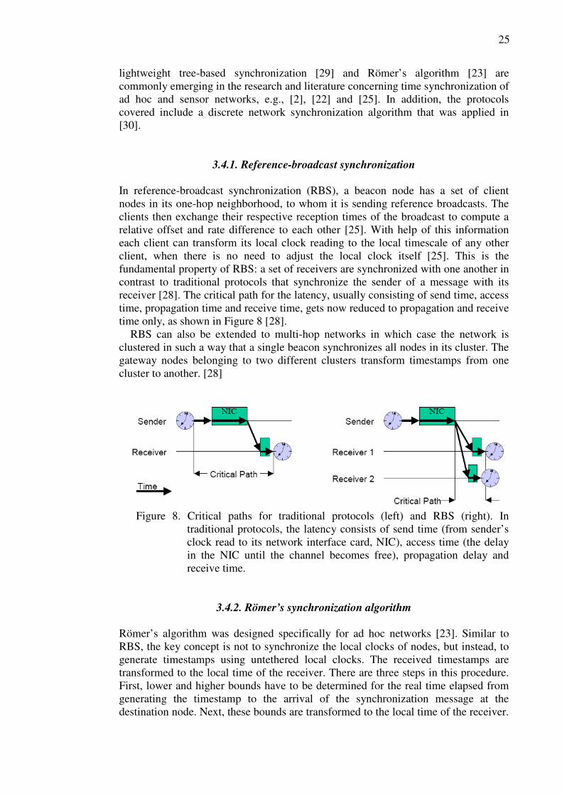
3.4.1. Reference-broadcast synchronization In reference-broadcast synchronization (RBS), a beacon node has a set of client nodes in its one-hop neighborhood, to whom it is sending reference broadcasts. The clients then exchange their respective reception times of the broadcast to compute a relative offset and rate difference to each other [25]. With help of this information each client can transform its local clock reading to the local timescale of any other client, when there is no need to adjust the local clock itself [25]. This is the fundamental property of RBS: a set of receivers are synchronized with one another in contrast to traditional protocols that synchronize the sender of a message with its receiver [28]. The critical path for the latency, usually consisting of send time, access time, propagation time and receive time, gets now reduced to propagation and receive time only, as shown in Figure 8 [28]. RBS can also be extended to multi-hop networks in which case the network is clustered in such a way that a single beacon synchronizes all nodes in its cluster. The gateway nodes belonging to two different clusters transform timestamps from one cluster to another. [28]

Figure 8. Critical paths for traditional protocols (left) and RBS (right). In

traditional protocols, the latency consists of send time (from sender’s clock read to its network interface card, NIC), access time (the delay in the NIC until the channel becomes free), propagation delay and receive time.

3.4.2. Römer’s synchronization algorithm Römer’s algorithm was designed specifically for ad hoc networks [23]. Similar to RBS, the key concept is not to synchronize the local clocks of nodes, but instead, to generate timestamps using untethered local clocks. The received timestamps are transformed to the local time of the receiver. There are three steps in this procedure. First, lower and higher bounds have to be determined for the real time elapsed from generating the timestamp to the arrival of the synchronization message at the destination node. Next, these bounds are transformed to the local time of the receiver.

26

Finally, these values are subtracted from the local time of arrival at the destination node resulting in a time interval that specifies lower and upper bounds for the timestamp relative to the local time of the receiver. The time difference is transformed from the local time of one node to the local time of another node with a specified time transformation formula. [22] Römer’s protocol is clearly designed with strict energy constraints in mind, because the clocks are running at their natural rates and, in addition to low resource usage and message overhead, the protocol utilizes a post-facto method that synchronizes the nodes only when an event of interest occurs. Furthermore, it supports multi-hop transmissions, but the synchronization error increases with the number of hops along the message path containing the timestamp. Another disadvantage is that the protocol requires a round-trip estimation which can increase the synchronization error. [22]

3.4.3. Lightweight tree-based synchronization Lightweight tree-based synchronization (LTS) does not aim for maximum precision, but focuses on minimizing overhead and energy while being robust and self-configuring [29]. LTS assumes one or more master nodes that are synchronized externally to a time reference. Using these master nodes, LTS synchronizes the nodes exploiting either on-demand or proactive algorithms. In the proactive method, a spanning tree with the masters at the root is constructed by flooding the network. With help of round-trip time calculations, each node synchronizes to its parent node in this tree. The synchronization frequency is calculated from the requested precision, depth of the spanning tree and drift bound. In the on-demand version, a node needing synchronization sends a request to one of the master nodes using any routing algorithm. All the nodes along the reverse path of the request message can synchronize themselves using round-trip measurements. The synchronization frequency is calculated as in the proactive version. [25] A disadvantage of LTS is that the synchronization error increases linearly with the depth of the tree [22].

3.4.4. Discrete network synchronization algorithm In [31], a discrete network synchronization algorithm is presented and analyzed. The algorithm is based on [32]. The purpose is to adjust a free running clock computationally with a correcting term that is obeying the recursive law

)1()(α)1( ++=+ khekckc iii , (5)

where α determines the amount of feedback (|α| < 1 is needed for stability), and h is a coefficient to weigh the current error measure ei. Values of 0.15 for α and 0.75 for h are proposed in [31]. The error measure ei in (5) is formed as an average

∑=

=+iN

j

ij

i

i keN

ke1

)(1

)1( , (6)

27

where eij is a calculated error between the ith node’s clock reading and the time reference in the received synchronization message from node j. Ni is the number of received synchronization messages at node i. The nodes exchange their clock information with each other at a certain time interval and adjust their clocks according to (5) and (6). Possible master nodes do not correct their clocks. The discrete network synchronization algorithm is a simple and robust internal synchronization method suitable for multi-hop sensor and ad hoc networks, where a common time reference needs to be maintained within the whole network. The algorithm can be used in both distributed and centralized systems.

28

4. FREQUENCY HOPPING A frequency hopping spread spectrum (FHSS) system is hopping from one frequency to another. It is one of the spread spectrum techniques where the original narrowband data are spread over a wider bandwidth by rapidly changing the frequency of the carrier signal. The information data are split into pieces of a certain size, and then transmitted over the frequency that the hopping pattern is currently pointing to. An example of such a pattern is presented in Figure 9, where each frequency hop is visited for the duration of the symbol time TS. Depending on the amount of the transmitted data on each hop, the FH-technique is called either fast frequency hopping (FFH) or slow frequency hopping (SFH). In FFH, less than one symbol is transferred on each frequency hop whereas an SFH system transmits one or more symbols per hop [13]. The duration of a hop is equal to the blank time (the time it takes to switch between two different frequencies) and the dwell time during which the channel symbols are actually transmitted [33].

Figure 9. An example of a frequency hopping pattern.

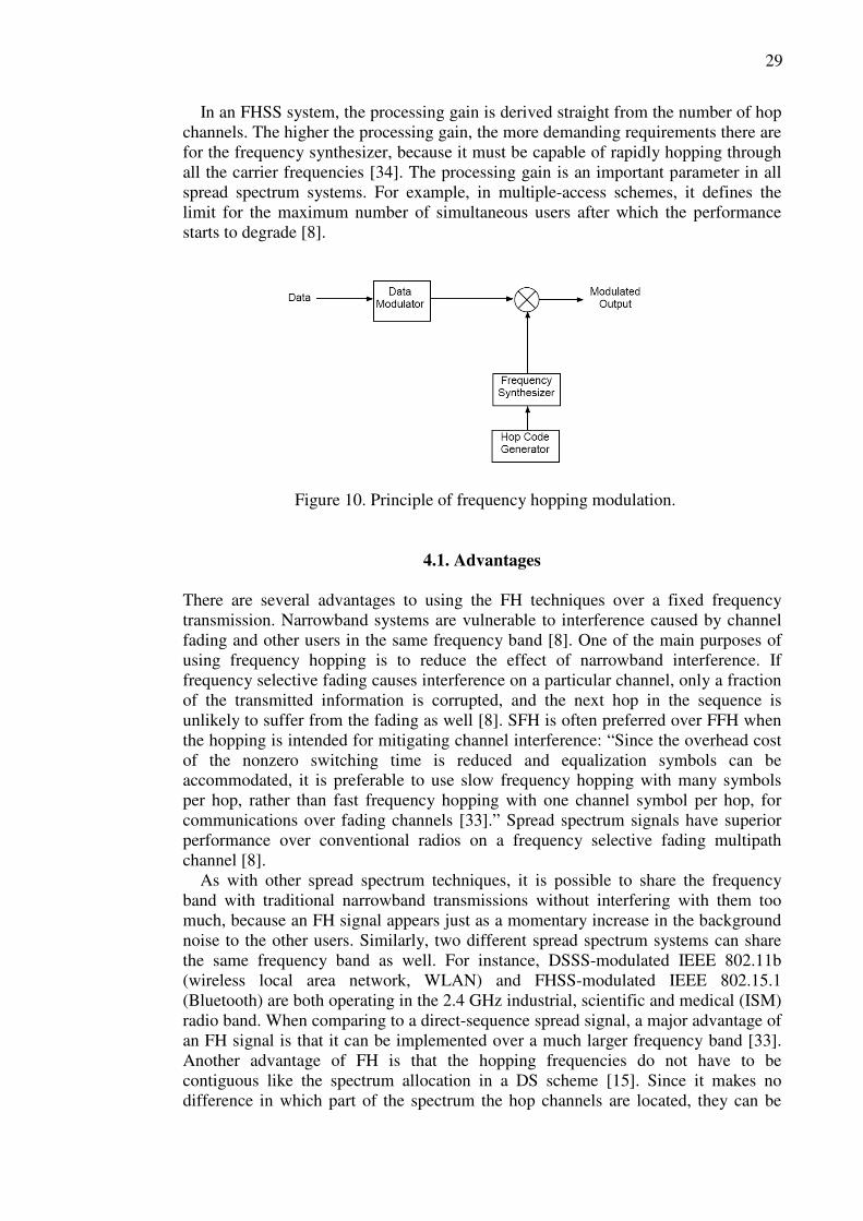
There is a two-part modulation process in the transmitter of an FHSS system. First, the data are modulated as in conventional transmitters. Non-coherent demodulation is usually required unless the hopping band is narrow [33]. The phase-coherence is difficult to maintain in FH systems due to the rapid synthesis of frequencies and the propagation of the signal over the channel as the signal hops from one frequency to another [13]. Good modulation candidates are, for example, differential phase-shift keying (DPSK), minimum-shift keying (MSK) or continuous-phase frequency-shift keying (CPFSK) [33]. The actual frequency hopping is the second modulation step, where a baseband signal is modulated to one of the channels according to a pseudo-random pattern from the PN-generator [13]. The two-step modulation structure is illustrated in Figure 10, in which the code generator controls the frequency synthesizer to output a corresponding carrier signal for the selected channel. The receiver can demodulate the signal by following the same hopping pattern as the transmitter. If the hopping is properly synchronized at both ends, a common logical channel is maintained. For outside users, the hopping appears as short-duration impulse noise.

4

3

6

5

F

requ

ency

0 TS 2TS 3TS 4TS 5TS 6TS Time

1

2

29

In an FHSS system, the processing gain is derived straight from the number of hop channels. The higher the processing gain, the more demanding requirements there are for the frequency synthesizer, because it must be capable of rapidly hopping through all the carrier frequencies [34]. The processing gain is an important parameter in all spread spectrum systems. For example, in multiple-access schemes, it defines the limit for the maximum number of simultaneous users after which the performance starts to degrade [8].

Figure 10. Principle of frequency hopping modulation.

4.1. Advantages There are several advantages to using the FH techniques over a fixed frequency transmission. Narrowband systems are vulnerable to interference caused by channel fading and other users in the same frequency band [8]. One of the main purposes of using frequency hopping is to reduce the effect of narrowband interference. If frequency selective fading causes interference on a particular channel, only a fraction of the transmitted information is corrupted, and the next hop in the sequence is unlikely to suffer from the fading as well [8]. SFH is often preferred over FFH when the hopping is intended for mitigating channel interference: “Since the overhead cost of the nonzero switching time is reduced and equalization symbols can be accommodated, it is preferable to use slow frequency hopping with many symbols per hop, rather than fast frequency hopping with one channel symbol per hop, for communications over fading channels [33].” Spread spectrum signals have superior performance over conventional radios on a frequency selective fading multipath channel [8]. As with other spread spectrum techniques, it is possible to share the frequency band with traditional narrowband transmissions without interfering with them too much, because an FH signal appears just as a momentary increase in the background noise to the other users. Similarly, two different spread spectrum systems can share the same frequency band as well. For instance, DSSS-modulated IEEE 802.11b (wireless local area network, WLAN) and FHSS-modulated IEEE 802.15.1 (Bluetooth) are both operating in the 2.4 GHz industrial, scientific and medical (ISM) radio band. When comparing to a direct-sequence spread signal, a major advantage of an FH signal is that it can be implemented over a much larger frequency band [33]. Another advantage of FH is that the hopping frequencies do not have to be contiguous like the spectrum allocation in a DS scheme [15]. Since it makes no difference in which part of the spectrum the hop channels are located, they can be

30

adaptively selected so that the channels located at interfered frequencies are completely left out of the hopping pattern. Adaptive frequency hopping (AFH) is implemented, for example, in Bluetooth [35]. FHSS is also extensively used in military communications to neutralize the effects of various types of intentional jamming and fading, and to improve the security as the transmissions are hard to intercept without knowing the correct FH pattern [36]. In the case of partial-band jamming, only a tiny part of the transmitted information is lost because the jammed frequency is visited for a very short period of time. A small number of bit errors can be easily recovered by using proper channel coding and interleaving [15]. However, the error coding methods might not be sufficient if a capable follower jammer is present. This type of jammer has the capability to determine which frequency slot of the bandwidth is currently used, and then create interfering signals in accordance with the hopping pattern [13]. One way to eliminate this problem is to use a very high hopping rate that prevents the jammer from having sufficient time to determine the hop frequency that is currently in use [13]. One advantage of frequency hopping comes from CDMA implementations where several users share a common bandwidth. FH CDMA is particularly attractive for mobile users because timing requirements are not as strict as in a DS spread signal [13]. If the hop sequences are time-synchronized, they can be selected to be orthogonal so that each user is transmitting at a different frequency band at any given time interval [15]. This holds true up to a certain limit in the number of users. Otherwise, collisions cannot be entirely avoided, but the hopping sequences can be selected in such a way that they are minimally correlated. Therefore, FH CDMA systems hardly suffer from the near-far effect at all, and the extensive power control usage required for DS systems is not needed [15].

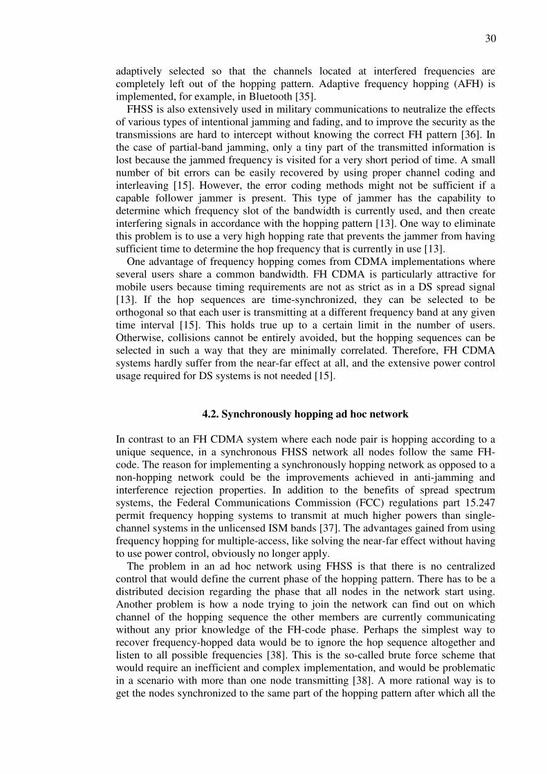
4.2. Synchronously hopping ad hoc network In contrast to an FH CDMA system where each node pair is hopping according to a unique sequence, in a synchronous FHSS network all nodes follow the same FH-code. The reason for implementing a synchronously hopping network as opposed to a non-hopping network could be the improvements achieved in anti-jamming and interference rejection properties. In addition to the benefits of spread spectrum systems, the Federal Communications Commission (FCC) regulations part 15.247 permit frequency hopping systems to transmit at much higher powers than single-channel systems in the unlicensed ISM bands [37]. The advantages gained from using frequency hopping for multiple-access, like solving the near-far effect without having to use power control, obviously no longer apply. The problem in an ad hoc network using FHSS is that there is no centralized control that would define the current phase of the hopping pattern. There has to be a distributed decision regarding the phase that all nodes in the network start using. Another problem is how a node trying to join the network can find out on which channel of the hopping sequence the other members are currently communicating without any prior knowledge of the FH-code phase. Perhaps the simplest way to recover frequency-hopped data would be to ignore the hop sequence altogether and listen to all possible frequencies [38]. This is the so-called brute force scheme that would require an inefficient and complex implementation, and would be problematic in a scenario with more than one node transmitting [38]. A more rational way is to get the nodes synchronized to the same part of the hopping pattern after which all the

31

nodes hop to the same frequency exactly at the same time. A few synchronization methods for achieving a common phase in ad hoc networks are described in the next section. The synchronization schemes usually assume that the hop sequence itself is known by all nodes beforehand, but the code phase is unknown. In various methods, the FH-code phase is derived from the local clock reading of a node. As previously explained in Chapters 3.2 and 3.4, clocks tend to drift from each other, meaning there has to be a time synchronization algorithm in place to correct the clock readings in order to guarantee the desired accuracy between the local clocks of nodes. This way, a common FH-code phase can be maintained within the network after the initial code phase acquisition.

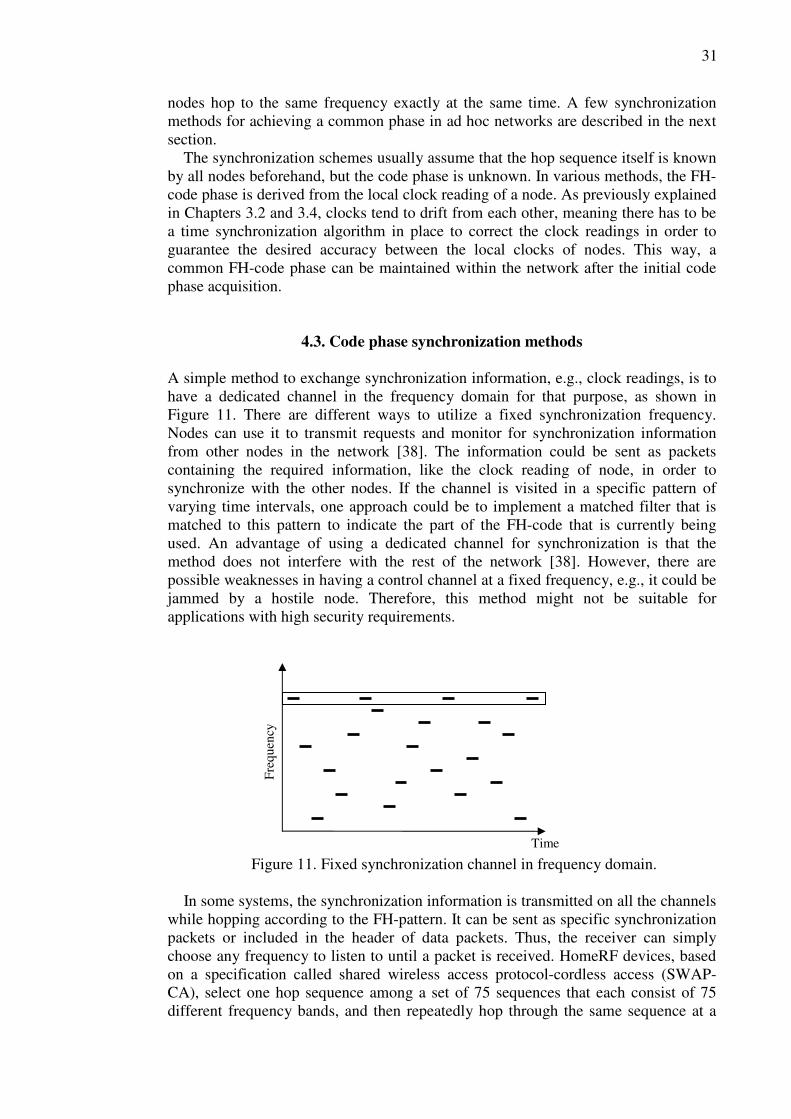
4.3. Code phase synchronization methods A simple method to exchange synchronization information, e.g., clock readings, is to have a dedicated channel in the frequency domain for that purpose, as shown in Figure 11. There are different ways to utilize a fixed synchronization frequency. Nodes can use it to transmit requests and monitor for synchronization information from other nodes in the network [38]. The information could be sent as packets containing the required information, like the clock reading of node, in order to synchronize with the other nodes. If the channel is visited in a specific pattern of varying time intervals, one approach could be to implement a matched filter that is matched to this pattern to indicate the part of the FH-code that is currently being used. An advantage of using a dedicated channel for synchronization is that the method does not interfere with the rest of the network [38]. However, there are possible weaknesses in having a control channel at a fixed frequency, e.g., it could be jammed by a hostile node. Therefore, this method might not be suitable for applications with high security requirements.

Figure 11. Fixed synchronization channel in frequency domain.

In some systems, the synchronization information is transmitted on all the channels while hopping according to the FH-pattern. It can be sent as specific synchronization packets or included in the header of data packets. Thus, the receiver can simply choose any frequency to listen to until a packet is received. HomeRF devices, based on a specification called shared wireless access protocol-cordless access (SWAP-CA), select one hop sequence among a set of 75 sequences that each consist of 75 different frequency bands, and then repeatedly hop through the same sequence at a

F

requ

ency

Time

32

rate of 50 hops per second in a total of 1.5 seconds [39]. In the network discovery phase, a node scans the network by listening on every channel for a specific amount of time, and receives all the packets regardless of network identifier (NWID) or destination address. The synchronization information is available in every data packet on the network, and therefore, a decision can be made whether or not to join a network by analyzing the incoming packets in the node’s MAC management module. When a network is found, the node synchronizes to the network by setting its hopping pattern to the discovered network’s hopping pattern. [39] However, the slow hops and repeating the same short code allow an eavesdropper to go through each channel and record the time of reception until the entire sequence is determined [40]. It should be noted that frequency hopping in HomeRF is not implemented to enhance security, but to comply with FCC regulations. A more secure approach is to use longer hop patterns that are only known by authorized users and share the time information that reveals the current phase. Nodes could be using a common time reference such as GPS to determine the current phase [38]. In [30], no external time references were used, but instead, the method implements a control channel in code-space that the transmitter is using for sending the synchronization information. The receiver can arbitrarily choose a frequency channel to listen to since each hop frequency is eventually covered with the required information. Additionally, the nodes periodically exchange synchronization messages containing timestamps in order to maintain the synchronism within the network. This FH-code phase synchronization method is thoroughly described in Chapter 5. Some FH-code phase synchronization methods are using two different hop sequences: one for synchronization and another for data transfers. A short sequence can be used for coarse code acquisition after which specific information is exchanged to synchronize with a longer hop sequence that is for normal data transfers [38]. Bluetooth has a slightly different kind of two-step synchronization process. There is a universal FH sequence for inquiry and a receiver specific point-to-point FH sequence for paging. During inquiry, senders discover and collect neighborhood information provided by receivers, whereas during paging, senders connect to the previously discovered receivers. In the beginning, the sender and the receiver will almost certainly be hopping in a different phase, because the current frequency hop is derived from the local clock reading of each node. The problem is solved so that the receiver changes hops at a much slower rate than the sender. After a short time, the sender is very likely to transmit at a frequency the receiver is currently listening to. Finally, the node assigned as the master sends its time information to the receiver who can then use it to adjust its clock. [41] From a security point of view, a divergent short synchronization sequence could be exposed if the synchronization transmissions are frequently repeated.

33

5. SYNCHRONIZATION METHOD If security is a high priority in an ad hoc network, good LPD, LPJ and LPI capabilities are required. These properties exist in systems using spread spectrum techniques such as direct sequence or frequency hopping with a high hopping rate. Further security improvements can be achieved by combining these two techniques. The problem in any FH ad hoc network is the synchronization of the nodes to the same hopping code phase since there is no common control in the network. Additionally, a robust system requires a very long hopping pattern having a period of days, weeks or even longer. Synchronizing such a long code, while satisfying the highest security requirements, is not an easy task by using conventional methods like a fixed synchronization frequency or a divergent synchronization sequence, which could both be exposed if the synchronization information is regularly transmitted. The whole synchronization procedure should always remain invisible to any unintended user. A novel method fulfilling the above-mentioned requirements is proposed in [30], where a comprehensive study is made of synchronizing a slow hopping FH / DSSS hybrid system in a multi-hop ad hoc network. In the paper, a series of simulations are run in an OPNET environment to prove that the proposed method functions properly in both a static and mobile scenarios even if low-cost quartz oscillators are being used. The applied time synchronization algorithm is able to keep the timing error at a satisfactory level as long as connectivity is good. For these reasons, the synchronization method presented in [30] is chosen to be implemented in this thesis. The method is put into practice with development boards that are later introduced in Chapter 6.

5.1. Control channel in code-space In ad hoc networks, the synchronization information has to be periodically broadcast in order to maintain synchronism throughout the network and provide a possibility for a new node to join and synchronize to the network in a reasonable period of time. In the mobile scenario of a time-synchronized network, the periodic broadcasting of synchronization messages is even more important because a node at the opposite side of the network can suddenly show up as a neighbor, in which case, even though technically synchronized, the nodes could have a significant time difference between their clock readings. When the network is also frequency hopping, the transmission of the synchronization information should be continuous in such a way that there is no need to derail from the hopping pattern and interrupt the data transmission. Typically, some kind of control channel is used. There are strict requirements for the control channel if security is a major concern; an outsider should not be able to detect, jam or intercept the transmission. In [30], the problem has been solved by putting the control channel in code-space and using a CDMA-like implementation of two different DS-spreading codes, similarly to the BCCA concept explained in Chapter 2.2.3. One spreading code is for synchronization transmissions and the other for data transmissions. The synchronization messages are DS-spread with a common synchronization code, denoted as DS(s)-code, which is known by every node. The simultaneous transmission of data packets and synchronization messages is possible because the

34

DS(s)-code is orthogonal to the spreading code used for data transmissions. Another benefit is the increased protection against interference and jamming due to the diversity obtained from extending the control channel to cover the entire frequency spectrum that is allocated for hopping. A jammer would have to be able to intensively follow the hopping pattern or jam all the channels in order to stop the synchronization process. Before the control channel can be used for exchanging synchronization information, the DS-code phase must be synchronized. Additionally, the timing of the frequency hops must be adjusted to get each hop-change to occur at the right time instant on both ends. These steps are accomplished via matched filtering.

5.2. Method description The synchronization signal consists of three parts. The first part is used to estimate the DS(s)-code phase and the second to set the FH-timing. After these two parts, the sender transmits a synchronization message including the time information needed for the receiver to synchronize to the FH-code phase since it is directly derived from the clock reading. The exact list of the functions of an unsynchronized node after powering up is defined in [30] as follows:

1. Listen to the three-part synchronization signal on a freely selected frequency channel. The waiting time depends on the synchronization message broadcast interval.

2. If no synchronization messages are received in during a predefined period of time, start following the FH-code at the point defined by the current clock reading.

3. Transmit the three-part synchronization message so that all hop frequencies are covered.

4. Go to the phase 1.

5.2.1. Transmitting the signal The transmitter makes sure that the whole three-part synchronization signal is eventually transmitted at all hop frequencies. Each part of the signal is sent on consecutive visits to that particular frequency the next time the FH-code is pointing to it. In Figure 12 [30], there are only three different frequency channels available. The hop sequence in question corresponds to {1, 3, 1, 2, 1, 2, 3, 3, 2}, which defines the time slots for sending out each part of the synchronization signal. For example, the second channel is first visited on the fourth hop when the DS(s)-code phase can be estimated at the receiving end. The next visit is on the sixth hop, where a pseudo-random training sequence is sent for FH-timing purposes. The bits in this training sequence are denoted as DS(fh)-chips. Although they have the same duration as information bits consisting of one DS(s)-code period, they are called chips because they do not carry any data. Finally, a synchronization message (MSG) with a clock reading is transmitted on the ninth hop after which the receiver learns the FH-code phase and is able to start following the hopping pattern. Although not illustrated in Figure 12, the possible data transmission is multiplexed into the signal with an orthogonal spreading code.

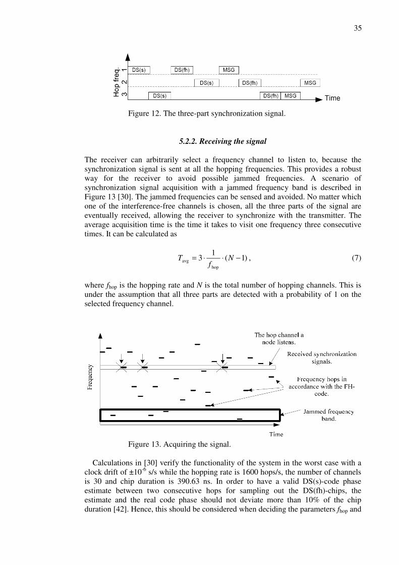
35

Figure 12. The three-part synchronization signal.

5.2.2. Receiving the signal The receiver can arbitrarily select a frequency channel to listen to, because the synchronization signal is sent at all the hopping frequencies. This provides a robust way for the receiver to avoid possible jammed frequencies. A scenario of synchronization signal acquisition with a jammed frequency band is described in Figure 13 [30]. The jammed frequencies can be sensed and avoided. No matter which one of the interference-free channels is chosen, all the three parts of the signal are eventually received, allowing the receiver to synchronize with the transmitter. The average acquisition time is the time it takes to visit one frequency three consecutive times. It can be calculated as

)1(1

3hop

avg −⋅⋅= Nf

T , (7)

where fhop is the hopping rate and N is the total number of hopping channels. This is under the assumption that all three parts are detected with a probability of 1 on the selected frequency channel.

Figure 13. Acquiring the signal.

Calculations in [30] verify the functionality of the system in the worst case with a clock drift of ±10-6 s/s while the hopping rate is 1600 hops/s, the number of channels is 30 and chip duration is 390.63 ns. In order to have a valid DS(s)-code phase estimate between two consecutive hops for sampling out the DS(fh)-chips, the estimate and the real code phase should not deviate more than 10% of the chip duration [42]. Hence, this should be considered when deciding the parameters fhop and

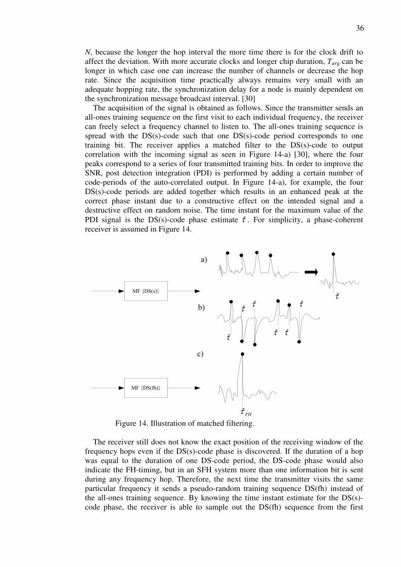
36

N, because the longer the hop interval the more time there is for the clock drift to affect the deviation. With more accurate clocks and longer chip duration, Tavg can be longer in which case one can increase the number of channels or decrease the hop rate. Since the acquisition time practically always remains very small with an adequate hopping rate, the synchronization delay for a node is mainly dependent on the synchronization message broadcast interval. [30] The acquisition of the signal is obtained as follows. Since the transmitter sends an all-ones training sequence on the first visit to each individual frequency, the receiver can freely select a frequency channel to listen to. The all-ones training sequence is spread with the DS(s)-code such that one DS(s)-code period corresponds to one training bit. The receiver applies a matched filter to the DS(s)-code to output correlation with the incoming signal as seen in Figure 14-a) [30], where the four peaks correspond to a series of four transmitted training bits. In order to improve the SNR, post detection integration (PDI) is performed by adding a certain number of code-periods of the auto-correlated output. In Figure 14-a), for example, the four DS(s)-code periods are added together which results in an enhanced peak at the correct phase instant due to a constructive effect on the intended signal and a destructive effect on random noise. The time instant for the maximum value of the PDI signal is the DS(s)-code phase estimate τ̂ . For simplicity, a phase-coherent receiver is assumed in Figure 14.

MF {DS(s)}

a)

b)

MF {DS(fh)}

τ̂

τ̂

τ̂τ̂

τ̂ τ̂

τ̂

c)

FHτ̂

Figure 14. Illustration of matched filtering. The receiver still does not know the exact position of the receiving window of the frequency hops even if the DS(s)-code phase is discovered. If the duration of a hop was equal to the duration of one DS-code period, the DS-code phase would also indicate the FH-timing, but in an SFH system more than one information bit is sent during any frequency hop. Therefore, the next time the transmitter visits the same particular frequency it sends a pseudo-random training sequence DS(fh) instead of the all-ones training sequence. By knowing the time instant estimate for the DS(s)-code phase, the receiver is able to sample out the DS(fh) sequence from the first

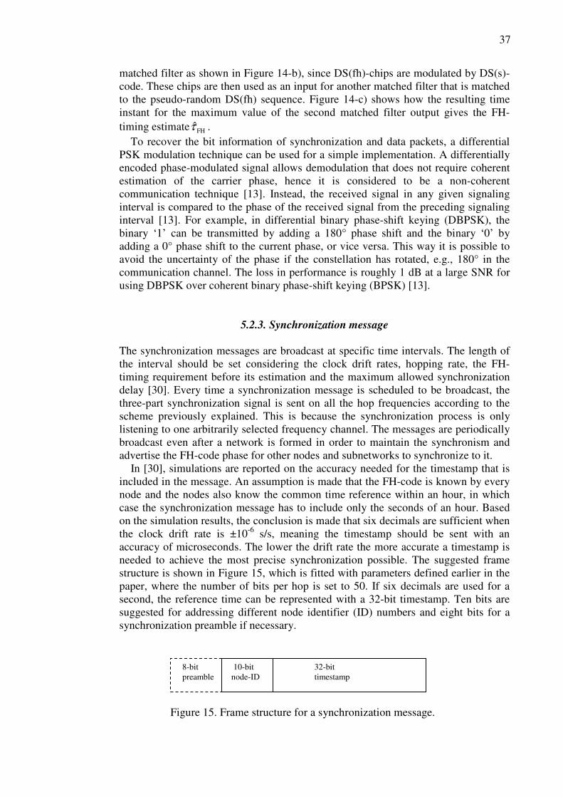
37

matched filter as shown in Figure 14-b), since DS(fh)-chips are modulated by DS(s)-code. These chips are then used as an input for another matched filter that is matched to the pseudo-random DS(fh) sequence. Figure 14-c) shows how the resulting time instant for the maximum value of the second matched filter output gives the FH-timing estimate FHτ̂ .

To recover the bit information of synchronization and data packets, a differential PSK modulation technique can be used for a simple implementation. A differentially encoded phase-modulated signal allows demodulation that does not require coherent estimation of the carrier phase, hence it is considered to be a non-coherent communication technique [13]. Instead, the received signal in any given signaling interval is compared to the phase of the received signal from the preceding signaling interval [13]. For example, in differential binary phase-shift keying (DBPSK), the binary ‘1’ can be transmitted by adding a 180° phase shift and the binary ‘0’ by adding a 0° phase shift to the current phase, or vice versa. This way it is possible to avoid the uncertainty of the phase if the constellation has rotated, e.g., 180° in the communication channel. The loss in performance is roughly 1 dB at a large SNR for using DBPSK over coherent binary phase-shift keying (BPSK) [13].

5.2.3. Synchronization message The synchronization messages are broadcast at specific time intervals. The length of the interval should be set considering the clock drift rates, hopping rate, the FH-timing requirement before its estimation and the maximum allowed synchronization delay [30]. Every time a synchronization message is scheduled to be broadcast, the three-part synchronization signal is sent on all the hop frequencies according to the scheme previously explained. This is because the synchronization process is only listening to one arbitrarily selected frequency channel. The messages are periodically broadcast even after a network is formed in order to maintain the synchronism and advertise the FH-code phase for other nodes and subnetworks to synchronize to it. In [30], simulations are reported on the accuracy needed for the timestamp that is included in the message. An assumption is made that the FH-code is known by every node and the nodes also know the common time reference within an hour, in which case the synchronization message has to include only the seconds of an hour. Based on the simulation results, the conclusion is made that six decimals are sufficient when the clock drift rate is ±10-6 s/s, meaning the timestamp should be sent with an accuracy of microseconds. The lower the drift rate the more accurate a timestamp is needed to achieve the most precise synchronization possible. The suggested frame structure is shown in Figure 15, which is fitted with parameters defined earlier in the paper, where the number of bits per hop is set to 50. If six decimals are used for a second, the reference time can be represented with a 32-bit timestamp. Ten bits are suggested for addressing different node identifier (ID) numbers and eight bits for a synchronization preamble if necessary.

Figure 15. Frame structure for a synchronization message.

8-bit preamble

32-bit timestamp

10-bit node-ID

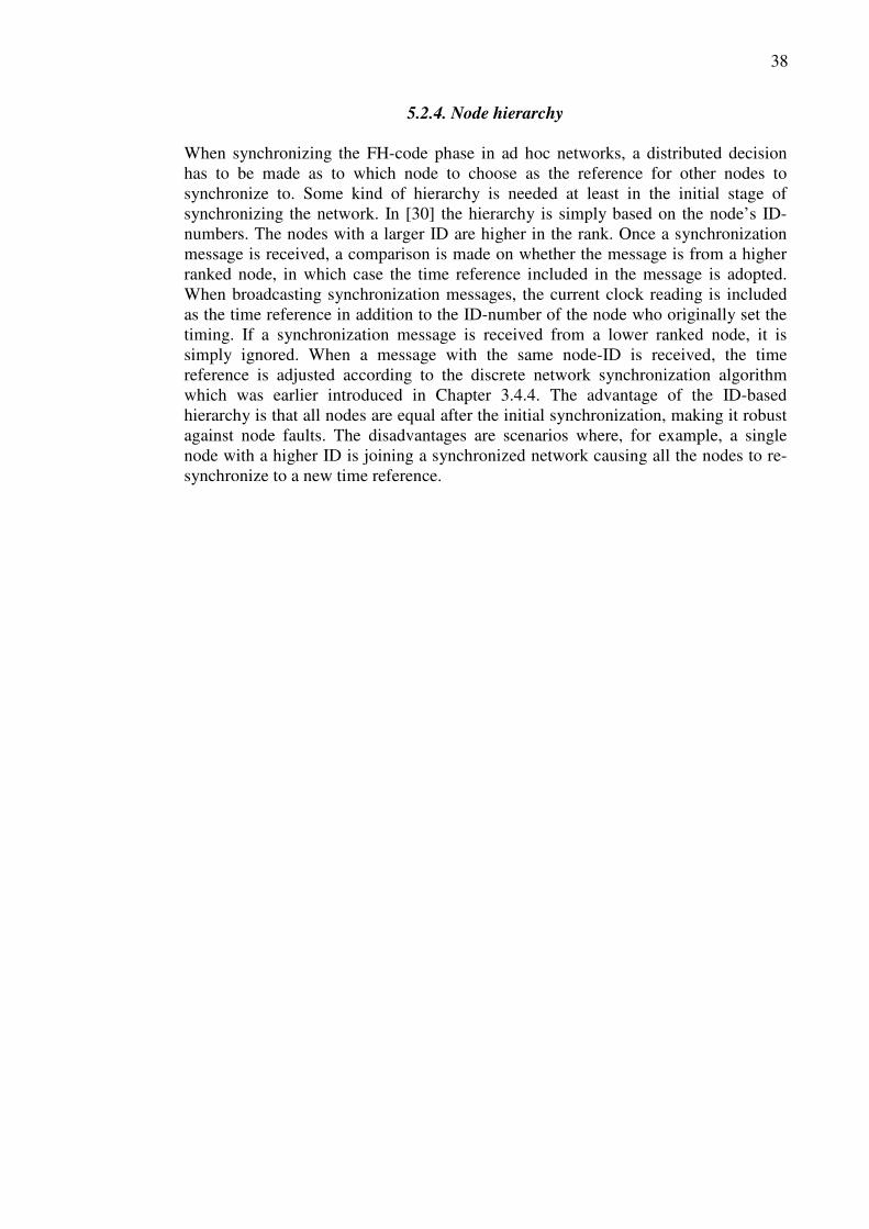
38

5.2.4. Node hierarchy When synchronizing the FH-code phase in ad hoc networks, a distributed decision has to be made as to which node to choose as the reference for other nodes to synchronize to. Some kind of hierarchy is needed at least in the initial stage of synchronizing the network. In [30] the hierarchy is simply based on the node’s ID-numbers. The nodes with a larger ID are higher in the rank. Once a synchronization message is received, a comparison is made on whether the message is from a higher ranked node, in which case the time reference included in the message is adopted. When broadcasting synchronization messages, the current clock reading is included as the time reference in addition to the ID-number of the node who originally set the timing. If a synchronization message is received from a lower ranked node, it is simply ignored. When a message with the same node-ID is received, the time reference is adjusted according to the discrete network synchronization algorithm which was earlier introduced in Chapter 3.4.4. The advantage of the ID-based hierarchy is that all nodes are equal after the initial synchronization, making it robust against node faults. The disadvantages are scenarios where, for example, a single node with a higher ID is joining a synchronized network causing all the nodes to re-synchronize to a new time reference.

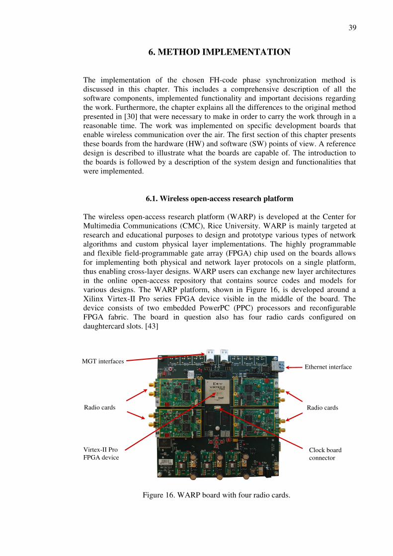
39

6. METHOD IMPLEMENTATION The implementation of the chosen FH-code phase synchronization method is discussed in this chapter. This includes a comprehensive description of all the software components, implemented functionality and important decisions regarding the work. Furthermore, the chapter explains all the differences to the original method presented in [30] that were necessary to make in order to carry the work through in a reasonable time. The work was implemented on specific development boards that enable wireless communication over the air. The first section of this chapter presents these boards from the hardware (HW) and software (SW) points of view. A reference design is described to illustrate what the boards are capable of. The introduction to the boards is followed by a description of the system design and functionalities that were implemented.

6.1. Wireless open-access research platform The wireless open-access research platform (WARP) is developed at the Center for Multimedia Communications (CMC), Rice University. WARP is mainly targeted at research and educational purposes to design and prototype various types of network algorithms and custom physical layer implementations. The highly programmable and flexible field-programmable gate array (FPGA) chip used on the boards allows for implementing both physical and network layer protocols on a single platform, thus enabling cross-layer designs. WARP users can exchange new layer architectures in the online open-access repository that contains source codes and models for various designs. The WARP platform, shown in Figure 16, is developed around a Xilinx Virtex-II Pro series FPGA device visible in the middle of the board. The device consists of two embedded PowerPC (PPC) processors and reconfigurable FPGA fabric. The board in question also has four radio cards configured on daughtercard slots. [43]

Figure 16. WARP board with four radio cards.

Virtex-II Pro FPGA device

Ethernet interface

Clock board connector

MGT interfaces

Radio cards Radio cards

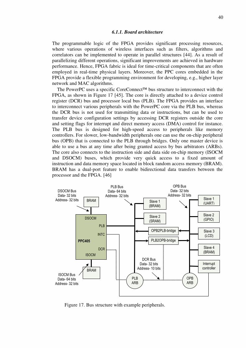
40

6.1.1. Board architecture The programmable logic of the FPGA provides significant processing resources, where various operations of wireless interfaces such as filters, algorithms and correlators can be implemented to operate in parallel structures [44]. As a result of parallelizing different operations, significant improvements are achieved in hardware performance. Hence, FPGA fabric is ideal for time-critical components that are often employed in real-time physical layers. Moreover, the PPC cores embedded in the FPGA provide a flexible programming environment for developing, e.g., higher layer network and MAC algorithms. The PowerPC uses a specific CoreConnect bus structure to interconnect with the FPGA, as shown in Figure 17 [45]. The core is directly attached to a device control register (DCR) bus and processor local bus (PLB). The FPGA provides an interface to interconnect various peripherals with the PowerPC core via the PLB bus, whereas the DCR bus is not used for transmitting data or instructions, but can be used to transfer device configuration settings by accessing DCR registers outside the core and setting flags for interrupt and direct memory access (DMA) control for instance. The PLB bus is designed for high-speed access to peripherals like memory controllers. For slower, low-bandwidth peripherals one can use the on-chip peripheral bus (OPB) that is connected to the PLB through bridges. Only one master device is able to use a bus at any time after being granted access by bus arbitrators (ARBs). The core also connects to the instruction side and data side on-chip memory (ISOCM and DSOCM) buses, which provide very quick access to a fixed amount of instruction and data memory space located in block random access memory (BRAM). BRAM has a dual-port feature to enable bidirectional data transfers between the processor and the FPGA. [46]

Figure 17. Bus structure with example peripherals.

PPC405

BRAM

BRAM Slave 1 (BRAM)

PLB ARB

Slave 2 (SRAM)

PLB2OPB-bridge

OPB ARB

ISOCM Bus Data- 64 bits

Address- 32 bits

PLB Bus Data- 64 bits

Address- 32 bits

DCR Bus Data- 32 bits

Address- 10 bits

DSOCM Bus Data- 32 bits

Address- 32 bits Slave 1 (UART)

Slave 2 (GPIO)

Slave 3 (LCD)

Interrupt controller

Slave 4 (BRAM)

OPB2PLB-bridge

PLB

INTC

DSOCM

ISOCM

DCR

OPB Bus Data- 32 bits

Address- 32 bits

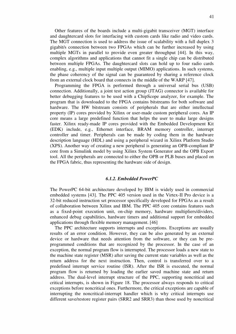
41

Other features of the boards include a multi-gigabit transceiver (MGT) interface and daughtercard slots for interfacing with custom cards like radio and video cards. The MGT connection is used to address the issue of scalability with a full duplex 3 gigabit/s connection between two FPGAs which can be further increased by using multiple MGTs in parallel to provide even greater throughput [44]. In this way, complex algorithms and applications that cannot fit a single chip can be distributed between multiple FPGAs. The daughtercard slots can hold up to four radio cards enabling, e.g., multiple input multiple output (MIMO) applications. In such systems, the phase coherency of the signal can be guaranteed by sharing a reference clock from an external clock board that connects in the middle of the WARP [47]. Programming the FPGA is performed through a universal serial bus (USB) connection. Additionally, a joint test action group (JTAG) connector is available for better debugging features to be used with a ChipScope analyzer, for example. The program that is downloaded to the FPGA contains bitstreams for both software and hardware. The HW bitstream consists of peripherals that are either intellectual property (IP) cores provided by Xilinx or user-made custom peripheral cores. An IP core means a large predefined function that helps the user to make large designs faster. Xilinx ready-made IP cores provided with the Embedded Development Kit (EDK) include, e.g., Ethernet interface, BRAM memory controller, interrupt controller and timer. Peripherals can be made by coding them in the hardware description language (HDL) and using a peripheral wizard in Xilinx Platform Studio (XPS). Another way of creating a new peripheral is generating an OPB-compliant IP core from a Simulink model by using Xilinx System Generator and the OPB Export tool. All the peripherals are connected to either the OPB or PLB buses and placed on the FPGA fabric, thus representing the hardware side of design.

6.1.2. Embedded PowerPC The PowerPC 64-bit architecture developed by IBM is widely used in commercial embedded systems [43]. The PPC 405 version used in the Virtex-II Pro device is a 32-bit reduced instruction set processor specifically developed for FPGAs as a result of collaboration between Xilinx and IBM. The PPC 405 core contains features such as a fixed-point execution unit, on-chip memory, hardware multipliers/dividers, enhanced debug capabilities, hardware timers and additional support for embedded applications through flexible memory management. [46] The PPC architecture supports interrupts and exceptions. Exceptions are usually results of an error condition. However, they can be also generated by an external device or hardware that needs attention from the software, or they can be pre-programmed conditions that are recognized by the processor. In the case of an exception, the normal program flow is interrupted. The processor loads a new state to the machine state register (MSR) after saving the current state variables as well as the return address for the next instruction. Then, control is transferred over to a predefined interrupt service routine (ISR). After the ISR is executed, the normal program flow is returned by loading the earlier saved machine state and return address. The dual-level interrupt structure of the PPC, supporting noncritical and critical interrupts, is shown in Figure 18. The processor always responds to critical exceptions before noncritical ones. Furthermore, the critical exceptions are capable of interrupting the noncritical-interrupt handler which is why critical interrupts use different save/restore register pairs (SRR2 and SRR3) than those used by noncritical

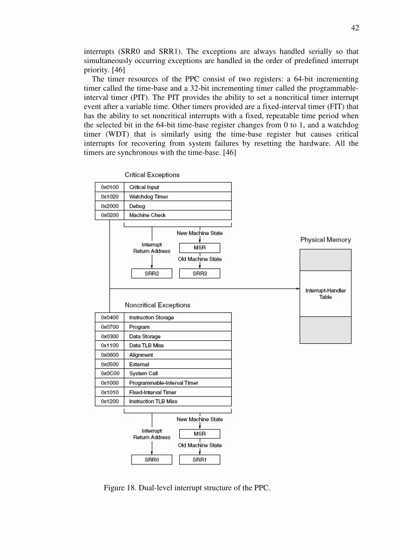
42

interrupts (SRR0 and SRR1). The exceptions are always handled serially so that simultaneously occurring exceptions are handled in the order of predefined interrupt priority. [46] The timer resources of the PPC consist of two registers: a 64-bit incrementing timer called the time-base and a 32-bit incrementing timer called the programmable-interval timer (PIT). The PIT provides the ability to set a noncritical timer interrupt event after a variable time. Other timers provided are a fixed-interval timer (FIT) that has the ability to set noncritical interrupts with a fixed, repeatable time period when the selected bit in the 64-bit time-base register changes from 0 to 1, and a watchdog timer (WDT) that is similarly using the time-base register but causes critical interrupts for recovering from system failures by resetting the hardware. All the timers are synchronous with the time-base. [46]

Figure 18. Dual-level interrupt structure of the PPC.

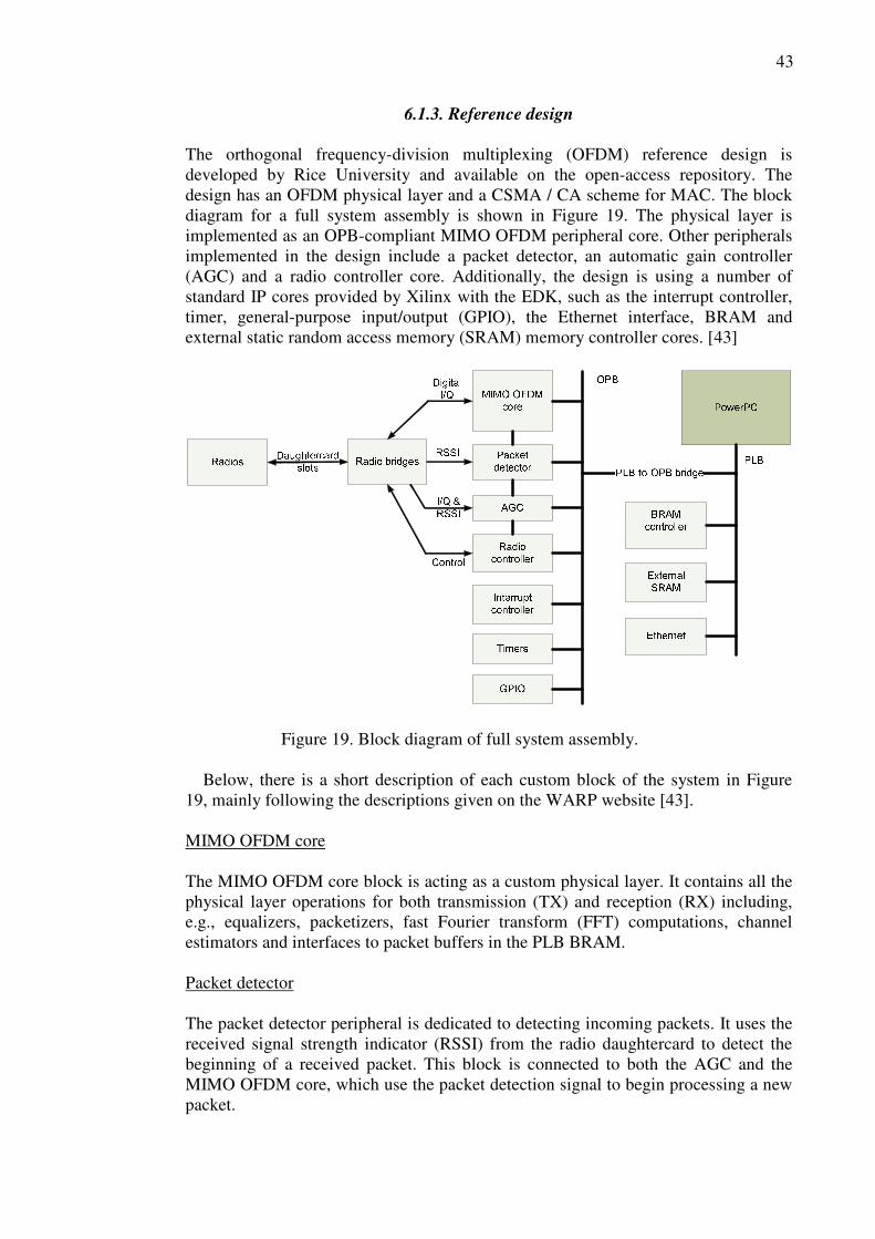
43

6.1.3. Reference design The orthogonal frequency-division multiplexing (OFDM) reference design is developed by Rice University and available on the open-access repository. The design has an OFDM physical layer and a CSMA / CA scheme for MAC. The block diagram for a full system assembly is shown in Figure 19. The physical layer is implemented as an OPB-compliant MIMO OFDM peripheral core. Other peripherals implemented in the design include a packet detector, an automatic gain controller (AGC) and a radio controller core. Additionally, the design is using a number of standard IP cores provided by Xilinx with the EDK, such as the interrupt controller, timer, general-purpose input/output (GPIO), the Ethernet interface, BRAM and external static random access memory (SRAM) memory controller cores. [43]

Figure 19. Block diagram of full system assembly. Below, there is a short description of each custom block of the system in Figure 19, mainly following the descriptions given on the WARP website [43]. MIMO OFDM core The MIMO OFDM core block is acting as a custom physical layer. It contains all the physical layer operations for both transmission (TX) and reception (RX) including, e.g., equalizers, packetizers, fast Fourier transform (FFT) computations, channel estimators and interfaces to packet buffers in the PLB BRAM. Packet detector The packet detector peripheral is dedicated to detecting incoming packets. It uses the received signal strength indicator (RSSI) from the radio daughtercard to detect the beginning of a received packet. This block is connected to both the AGC and the MIMO OFDM core, which use the packet detection signal to begin processing a new packet.

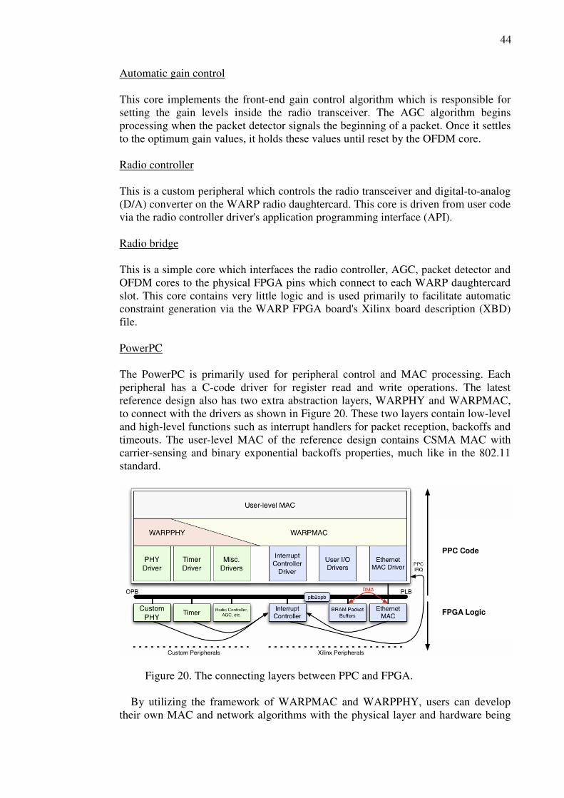
44

Automatic gain control This core implements the front-end gain control algorithm which is responsible for setting the gain levels inside the radio transceiver. The AGC algorithm begins processing when the packet detector signals the beginning of a packet. Once it settles to the optimum gain values, it holds these values until reset by the OFDM core. Radio controller This is a custom peripheral which controls the radio transceiver and digital-to-analog (D/A) converter on the WARP radio daughtercard. This core is driven from user code via the radio controller driver's application programming interface (API). Radio bridge This is a simple core which interfaces the radio controller, AGC, packet detector and OFDM cores to the physical FPGA pins which connect to each WARP daughtercard slot. This core contains very little logic and is used primarily to facilitate automatic constraint generation via the WARP FPGA board's Xilinx board description (XBD) file. PowerPC The PowerPC is primarily used for peripheral control and MAC processing. Each peripheral has a C-code driver for register read and write operations. The latest reference design also has two extra abstraction layers, WARPHY and WARPMAC, to connect with the drivers as shown in Figure 20. These two layers contain low-level and high-level functions such as interrupt handlers for packet reception, backoffs and timeouts. The user-level MAC of the reference design contains CSMA MAC with carrier-sensing and binary exponential backoffs properties, much like in the 802.11 standard.

Figure 20. The connecting layers between PPC and FPGA. By utilizing the framework of WARPMAC and WARPPHY, users can develop their own MAC and network algorithms with the physical layer and hardware being

PPC Code

FPGA Logic

45

abstracted away. For example, it is likely that novel random-access MAC can directly utilize the high-level function of the framework for binary exponential backoff to deal with medium contention [48]. With more complex algorithms, the user may need to dig deeper into the low-level functions and drivers, or create completely new peripherals on the FPGA in order to satisfy the requirements for the algorithms. For example, time-consuming components can be hardware accelerated by moving some parts of the functional modules from SW to HW. The FPGA has dedicated multipliers for fast and efficient multiplication, and this way it is possible to optimize the performance of functions that are taking a lot of CPU time.

6.2. System design The purpose of this work is to implement and demonstrate the FH-code phase synchronization method on the WARP development boards. The OFDM reference design is functioning as a basis, which needs to be further enhanced with both frequency hopping and control channel functionalities in order to provide a correct type of environment for demonstrating the synchronization method. Although the topic is a synchronization method aimed at the MANET category of networks where energy constraints are usually very important, this aspect is not considered in this implementation. Furthermore, the WARP setup used contains only one radio card per board. This means that it is not possible to simultaneously listen to two different channels, which is a feature that would be needed in a scenario of multiple nodes; after two nodes have been successfully synchronized, the freely selected synchronization channel should be listened to for further synchronization transmissions from other nodes while, at the same, hopping according to the hopping sequence. Otherwise, nodes that have a lower ID are still able to join the already formed network, but any node with a higher ID gets ignored since the network cannot receive out-of-phase transmissions. Therefore, a scenario of two nodes is primarily considered in this implementation, although multi-node scenarios are possible when carefully organized. Mainly two different approaches were considered for the top level design of the implementation. First, the synchronization module could be implemented as a separate process which is running in parallel to the MAC module. This would allow MAC to handle the synchronization packets at the most convenient time for it. The second, less complex approach is to entirely integrate the synchronization process to be a part of MAC, which might have the drawback of slowing MAC down. In the final implementation, the synchronization process is a mixture of both of these approaches being partly embedded with MAC while some functions are executed in a parallel fashion through interrupts. Because only one PowerPC processor is configured for the system, truly parallel processes are not possible. However, virtually parallel processes could be implemented with one processor by using the threading functionality provided with a real-time operating system (RTOS) such as Xilinx Xilkernel that is supported by the Virtex-II Pro. The PowerPC version of Xilkernel has various functionalities like threading, mutual exclusive (mutex) locks, semaphore locks, shared memory, dynamic memory and message queues [49]. Considering these properties, especially threading and message queues, Xilkernel would make a very suitable operating system (OS) for the work as done in this thesis. Since a thread is not necessarily linearly processed as opposed to conventional programming, two parallel finite state machines (FSMs) are possible, e.g., one thread

46

for MAC and another for the synchronization process. Any extra processes such as a routing module could be added simply by creating another thread. However, the drawback of Xilkernel is the complexity of its interrupt framework which is partly the reason why the reference design is using the standalone board support package (BSP), meaning no OS is being used [43]. The scope of this work does not include a custom physical layer implementation that would support both frequency hopping and direct-sequence spreading. Instead, alternative approaches to conventional hardware physical layers are used to accomplish the same functionalities. The implementation of the frequency hopping functionality is completely interrupt-driven from the PowerPC by switching the frequency channels in a specific interrupt service routine that utilizes a radio controller command to set the correct channel. The routine also keeps frequencykeeping hop windows synchronized between the nodes. Instead of using DS-spreading to form a control channel in code-space, the MAC frame payload is modified so that it is possible to send data and synchronization packets simultaneously. This way the original physical layer implementation can remain untouched, yet a sufficient environment is achieved for demonstrating the FH-code phase synchronization method.

6.2.1. Implementation requirements

The reference design provides basic functionality of MAC and PHY. All the additional requirements for the implementation are outlined as follows. First, the frequency hopping functionality must be implemented. A finite state machine is needed for the synchronization process consisting of at least two states: an initialization state where one freely selected frequency channel is listened to and a synchronized state where frequency hopping is enabled and both synchronization and data packets are exchanged. Functionality is needed for scheduling events such as transmitting a synchronization packet at certain time intervals, recognizing various timeouts and changing between the initialization state and the synchronized state. In order to maintain the synchronism throughout the network, a time synchronization algorithm is applied. Thus, the system must be able to frequently adjust and change its clock reading while synchronization packets are being received. Furthermore, the FH-code phase must be directly derived from the clock reading and the hop-changes must be adjusted to occur at the same time instant between all nodes. When transmitting, the possible scenario of simultaneous transmission of both data and synchronization packets must be addressed by multiplexing the packets together. Timestamping of synchronization packets should be performed at the very latest possible time instant prior to transmission. The reception time of a packet should be recorded at the receiver so that any delays caused by the MAC packet handling process can be calculated and added to the timestamp.

6.2.2. Medium access control process

The CSMA/CA MAC that comes along with the reference design can be utilized in this work to some extent. However, a few additions are required so that the MAC process would be able to properly handle incoming and outgoing synchronization messages. As stated in the requirements, the timestamping of outgoing messages

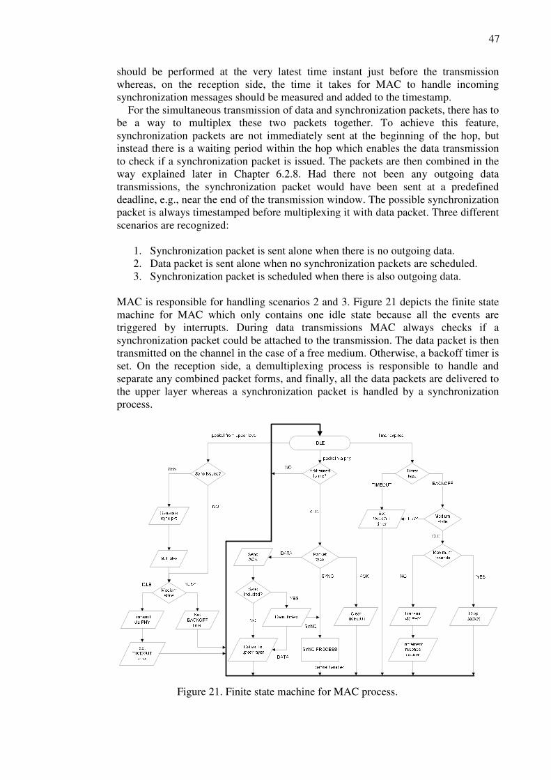
47

should be performed at the very latest time instant just before the transmission whereas, on the reception side, the time it takes for MAC to handle incoming synchronization messages should be measured and added to the timestamp. For the simultaneous transmission of data and synchronization packets, there has to be a way to multiplex these two packets together. To achieve this feature, synchronization packets are not immediately sent at the beginning of the hop, but instead there is a waiting period within the hop which enables the data transmission to check if a synchronization packet is issued. The packets are then combined in the way explained later in Chapter 6.2.8. Had there not been any outgoing data transmissions, the synchronization packet would have been sent at a predefined deadline, e.g., near the end of the transmission window. The possible synchronization packet is always timestamped before multiplexing it with data packet. Three different scenarios are recognized:

1. Synchronization packet is sent alone when there is no outgoing data. 2. Data packet is sent alone when no synchronization packets are scheduled. 3. Synchronization packet is scheduled when there is also outgoing data.

MAC is responsible for handling scenarios 2 and 3. Figure 21 depicts the finite state machine for MAC which only contains one idle state because all the events are triggered by interrupts. During data transmissions MAC always checks if a synchronization packet could be attached to the transmission. The data packet is then transmitted on the channel in the case of a free medium. Otherwise, a backoff timer is set. On the reception side, a demultiplexing process is responsible to handle and separate any combined packet forms, and finally, all the data packets are delivered to the upper layer whereas a synchronization packet is handled by a synchronization process.

Figure 21. Finite state machine for MAC process.

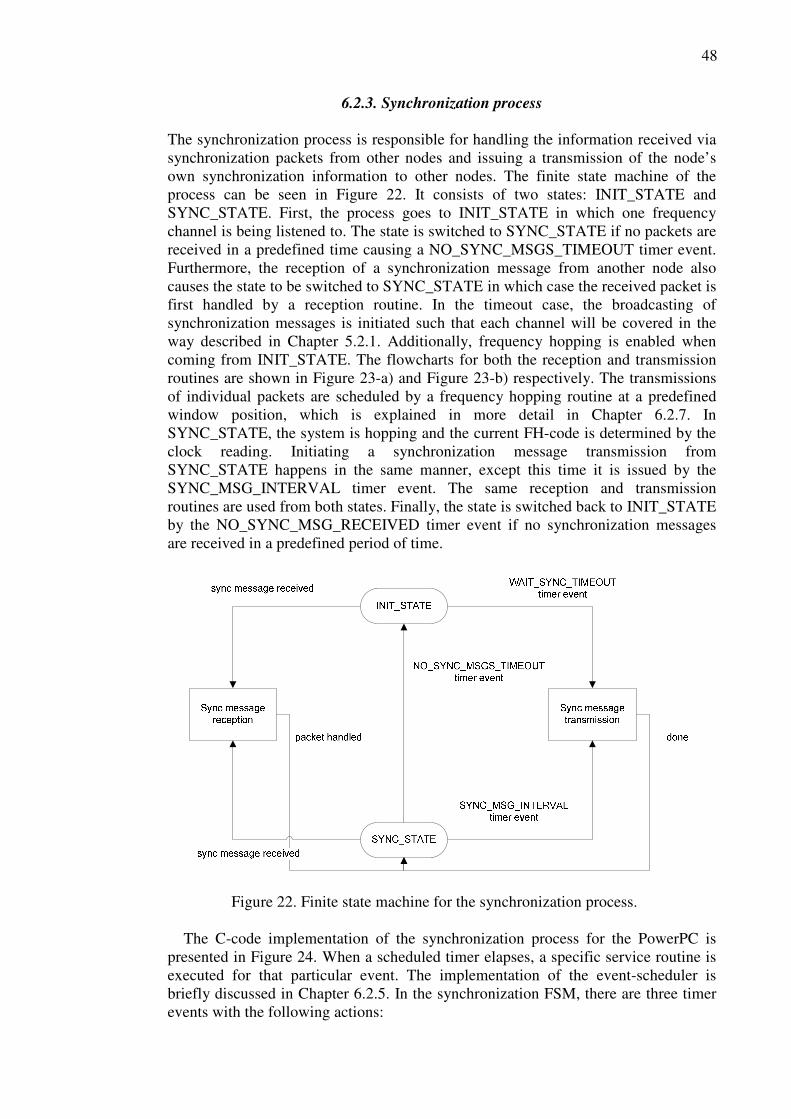
48

6.2.3. Synchronization process The synchronization process is responsible for handling the information received via synchronization packets from other nodes and issuing a transmission of the node’s own synchronization information to other nodes. The finite state machine of the process can be seen in Figure 22. It consists of two states: INIT_STATE and SYNC_STATE. First, the process goes to INIT_STATE in which one frequency channel is being listened to. The state is switched to SYNC_STATE if no packets are received in a predefined time causing a NO_SYNC_MSGS_TIMEOUT timer event. Furthermore, the reception of a synchronization message from another node also causes the state to be switched to SYNC_STATE in which case the received packet is first handled by a reception routine. In the timeout case, the broadcasting of synchronization messages is initiated such that each channel will be covered in the way described in Chapter 5.2.1. Additionally, frequency hopping is enabled when coming from INIT_STATE. The flowcharts for both the reception and transmission routines are shown in Figure 23-a) and Figure 23-b) respectively. The transmissions of individual packets are scheduled by a frequency hopping routine at a predefined window position, which is explained in more detail in Chapter 6.2.7. In SYNC_STATE, the system is hopping and the current FH-code is determined by the clock reading. Initiating a synchronization message transmission from SYNC_STATE happens in the same manner, except this time it is issued by the SYNC_MSG_INTERVAL timer event. The same reception and transmission routines are used from both states. Finally, the state is switched back to INIT_STATE by the NO_SYNC_MSG_RECEIVED timer event if no synchronization messages are received in a predefined period of time.

Figure 22. Finite state machine for the synchronization process.

The C-code implementation of the synchronization process for the PowerPC is presented in Figure 24. When a scheduled timer elapses, a specific service routine is executed for that particular event. The implementation of the event-scheduler is briefly discussed in Chapter 6.2.5. In the synchronization FSM, there are three timer events with the following actions:

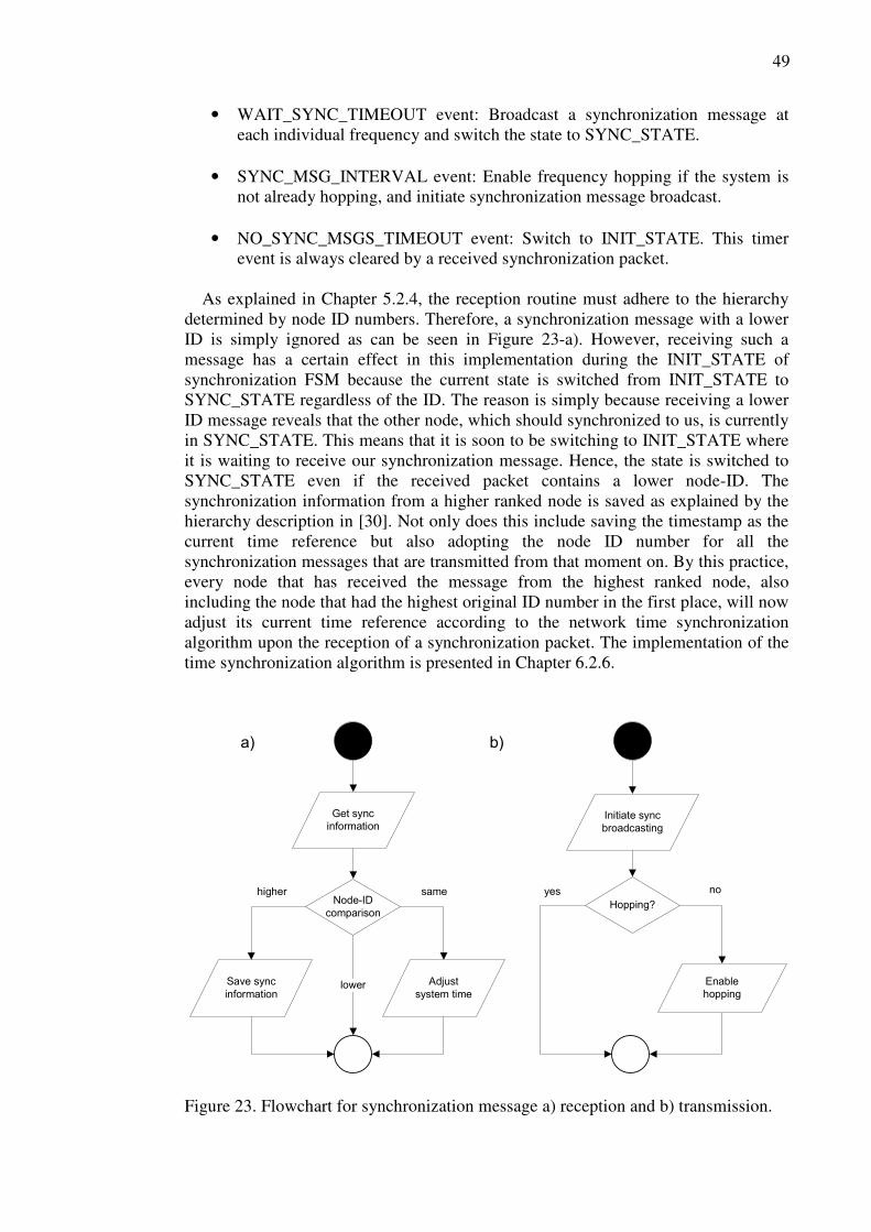
49

• WAIT_SYNC_TIMEOUT event: Broadcast a synchronization message at each individual frequency and switch the state to SYNC_STATE.

• SYNC_MSG_INTERVAL event: Enable frequency hopping if the system is

not already hopping, and initiate synchronization message broadcast.

• NO_SYNC_MSGS_TIMEOUT event: Switch to INIT_STATE. This timer event is always cleared by a received synchronization packet.

As explained in Chapter 5.2.4, the reception routine must adhere to the hierarchy determined by node ID numbers. Therefore, a synchronization message with a lower ID is simply ignored as can be seen in Figure 23-a). However, receiving such a message has a certain effect in this implementation during the INIT_STATE of synchronization FSM because the current state is switched from INIT_STATE to SYNC_STATE regardless of the ID. The reason is simply because receiving a lower ID message reveals that the other node, which should synchronized to us, is currently in SYNC_STATE. This means that it is soon to be switching to INIT_STATE where it is waiting to receive our synchronization message. Hence, the state is switched to SYNC_STATE even if the received packet contains a lower node-ID. The synchronization information from a higher ranked node is saved as explained by the hierarchy description in [30]. Not only does this include saving the timestamp as the current time reference but also adopting the node ID number for all the synchronization messages that are transmitted from that moment on. By this practice, every node that has received the message from the highest ranked node, also including the node that had the highest original ID number in the first place, will now adjust its current time reference according to the network time synchronization algorithm upon the reception of a synchronization packet. The implementation of the time synchronization algorithm is presented in Chapter 6.2.6.

Get sync

information

Node-ID

comparison

Adjust

system time

Save sync

information

higher

lower

same

Initiate sync

broadcasting

a) b)

Hopping?

yes

Enable

hopping

no

Figure 23. Flowchart for synchronization message a) reception and b) transmission.

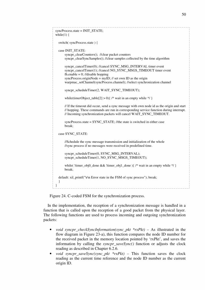
50

Figure 24. C-coded FSM for the synchronization process.

In the implementation, the reception of a synchronization message is handled in a function that is called upon the reception of a good packet from the physical layer. The following functions are used to process incoming and outgoing synchronization packets:

• void syncpr_checkSyncInformation(sync_pkt *rxPkt) – As illustrated in the flow diagram in Figure 23-a), this function compares the node ID number for the received packet in the memory location pointed by ‘rxPkt’, and saves the information by calling the syncpr_saveSync() function or adjusts the clock reading as described in Chapter 6.2.6.

• void syncpr_saveSync(sync_pkt *rxPkt) – This function saves the clock reading as the current time reference and the node ID number as the current origin ID.

syncProcess.state = INIT_STATE; while(1) {

switch( syncProcess.state ) { case INIT_STATE:

syncpr_clearCounters(); //clear packet counters syncpr_clearSyncSamples(); //clear samples collected by the time algorithm syncpr_cancelTimer(0); //cancel SYNC_MSG_INTERVAL timer event syncpr_cancelTimer(1); //cancel NO_SYNC_MSGS_TIMEOUT timer event fh.enable = 0; //disable hopping syncProcess.originNode = myID; // set own ID as the origin warpmac_setChannel(syncProcess.channel); //select synchronization channel syncpr_scheduleTimer(2, WAIT_SYNC_TIMEOUT); while(timerObject_table[2] > 0){ /* wait in an empty while */ } // If the timeout did occur, send a sync message with own node id as the origin and start // hopping. These commands are run in corresponding service function during interrupt. // Incoming synchronization packets will cancel WAIT_SYNC_TIMEOUT. syncProcess.state = SYNC_STATE; //the state is switched in either case break;

case SYNC_STATE:

//Schedule the sync message transmission and initialization of the whole //sync process if no messages were received in predefined time. syncpr_scheduleTimer(0, SYNC_MSG_INTERVAL); syncpr_scheduleTimer(1, NO_SYNC_MSGS_TIMEOUT); while( !timer_obj0_done && !timer_obj1_done ){ /* wait in an empty while */ } break;

default: xil_printf("\r\n Error state in the FSM of sync process"); break; }

}

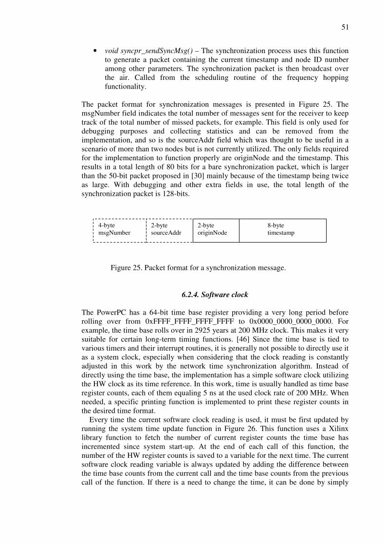
51

• void syncpr_sendSyncMsg() – The synchronization process uses this function to generate a packet containing the current timestamp and node ID number among other parameters. The synchronization packet is then broadcast over the air. Called from the scheduling routine of the frequency hopping functionality.

The packet format for synchronization messages is presented in Figure 25. The msgNumber field indicates the total number of messages sent for the receiver to keep track of the total number of missed packets, for example. This field is only used for debugging purposes and collecting statistics and can be removed from the implementation, and so is the sourceAddr field which was thought to be useful in a scenario of more than two nodes but is not currently utilized. The only fields required for the implementation to function properly are originNode and the timestamp. This results in a total length of 80 bits for a bare synchronization packet, which is larger than the 50-bit packet proposed in [30] mainly because of the timestamp being twice as large. With debugging and other extra fields in use, the total length of the synchronization packet is 128-bits.

Figure 25. Packet format for a synchronization message.

6.2.4. Software clock The PowerPC has a 64-bit time base register providing a very long period before rolling over from 0xFFFF_FFFF_FFFF_FFFF to 0x0000_0000_0000_0000. For example, the time base rolls over in 2925 years at 200 MHz clock. This makes it very suitable for certain long-term timing functions. [46] Since the time base is tied to various timers and their interrupt routines, it is generally not possible to directly use it as a system clock, especially when considering that the clock reading is constantly adjusted in this work by the network time synchronization algorithm. Instead of directly using the time base, the implementation has a simple software clock utilizing the HW clock as its time reference. In this work, time is usually handled as time base register counts, each of them equaling 5 ns at the used clock rate of 200 MHz. When needed, a specific printing function is implemented to print these register counts in the desired time format. Every time the current software clock reading is used, it must be first updated by running the system time update function in Figure 26. This function uses a Xilinx library function to fetch the number of current register counts the time base has incremented since system start-up. At the end of each call of this function, the number of the HW register counts is saved to a variable for the next time. The current software clock reading variable is always updated by adding the difference between the time base counts from the current call and the time base counts from the previous call of the function. If there is a need to change the time, it can be done by simply

4-byte msgNumber

2-byte sourceAddr

2-byte originNode

8-byte timestamp

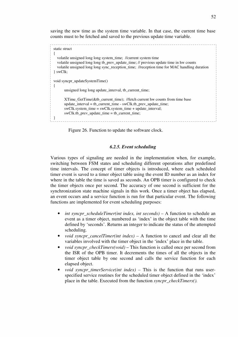
52

saving the new time as the system time variable. In that case, the current time base counts must to be fetched and saved to the previous update time variable.

Figure 26. Function to update the software clock.

6.2.5. Event scheduling Various types of signaling are needed in the implementation when, for example, switching between FSM states and scheduling different operations after predefined time intervals. The concept of timer objects is introduced, where each scheduled timer event is saved to a timer object table using the event ID number as an index for where in the table the time is saved as seconds. An OPB timer is configured to check the timer objects once per second. The accuracy of one second is sufficient for the synchronization state machine signals in this work. Once a timer object has elapsed, an event occurs and a service function is run for that particular event. The following functions are implemented for event scheduling purposes:

• int syncpr_scheduleTimer(int index, int seconds) – A function to schedule an event as a timer object, numbered as ‘index’ in the object table with the time defined by ‘seconds’. Returns an integer to indicate the status of the attempted scheduling.

• void syncpr_cancelTimer(int index) – A function to cancel and clear all the variables involved with the timer object in the ‘index’ place in the table.

• void syncpr_checkTimers(void) – This function is called once per second from the ISR of the OPB timer. It decrements the times of all the objects in the timer object table by one second and calls the service function for each elapsed object.

• void syncpr_timerService(int index) – This is the function that runs user-specified service routines for the scheduled timer object defined in the ‘index’ place in the table. Executed from the function syncpr_checkTimers().

static struct {

volatile unsigned long long system_time; //current system time volatile unsigned long long tb_prev_update_time; // previous update time in hw counts volatile unsigned long long sync_reception_time; //reception time for MAC handling duration

} swClk; void syncpr_updateSystemTime() {

unsigned long long update_interval, tb_current_time; XTime_GetTime(&tb_current_time); //fetch current hw counts from time base update_interval = tb_current_time - swClk.tb_prev_update_time; swClk.system_time = swClk.system_time + update_interval; swClk.tb_prev_update_time = tb_current_time;

}

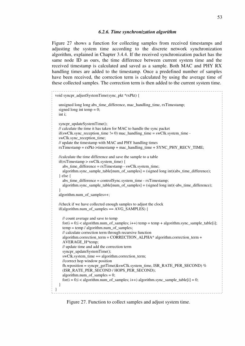
53

6.2.6. Time synchronization algorithm Figure 27 shows a function for collecting samples from received timestamps and adjusting the system time according to the discrete network synchronization algorithm, explained in Chapter 3.4.4. If the received synchronization packet has the same node ID as ours, the time difference between current system time and the received timestamp is calculated and saved as a sample. Both MAC and PHY RX handling times are added to the timestamp. Once a predefined number of samples have been received, the correction term is calculated by using the average time of these collected samples. The correction term is then added to the current system time.

Figure 27. Function to collect samples and adjust system time.

void syncpr_adjustSystemTime(sync_pkt *rxPkt) {

unsigned long long abs_time_difference, mac_handling_time, rxTimestamp; signed long int temp = 0; int i; syncpr_updateSystemTime(); // calculate the time it has taken for MAC to handle the sync packet if(swClk.sync_reception_time != 0) mac_handling_time = swClk.system_time - swClk.sync_reception_time; // update the timestamp with MAC and PHY handling times rxTimestamp = rxPkt->timestamp + mac_handling_time + SYNC_PHY_RECV_TIME; //calculate the time difference and save the sample to a table if(rxTimestamp > swClk.system_time) {

abs_time_difference = rxTimestamp - swClk.system_time; algorithm.sync_sample_table[num_of_samples] = (signed long int)(abs_time_difference);

} else { abs_time_difference = controlSync.system_time - rxTimestamp; algorithm.sync_sample_table[num_of_samples] = (signed long int)(-abs_time_difference);

} algorithm.num_of_samples++; //check if we have collected enough samples to adjust the clock if(algorithm.num_of_samples == AVG_SAMPLES) {

// count average and save to temp for(i = 0;i < algorithm.num_of_samples; i++) temp = temp + algorithm.sync_sample_table[i]; temp = temp / algorithm.num_of_samples; // calculate correction term through recursive function algorithm.correction_term = CORRECTION_ALPHA* algorithm.correction_term + AVERAGE_H*temp; // update time and add the correction term syncpr_updateSystemTime(); swClk.system_time += algorithm.correction_term; //correct hop window position fh.wposition = syncpr_getTime(&swClk.system_time, ISR_RATE_PER_SECOND) % (ISR_RATE_PER_SECOND / HOPS_PER_SECOND); algorithm.num_of_samples = 0; for(i = 0;i < algorithm.num_of_samples; i++) algorithm.sync_sample_table[i] = 0;

} }

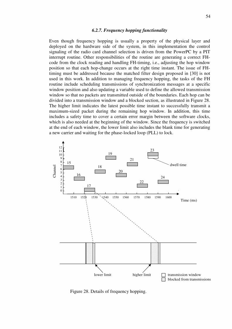
54

6.2.7. Frequency hopping functionality Even though frequency hopping is usually a property of the physical layer and deployed on the hardware side of the system, in this implementation the control signaling of the radio card channel selection is driven from the PowerPC by a PIT interrupt routine. Other responsibilities of the routine are generating a correct FH-code from the clock reading and handling FH-timing, i.e., adjusting the hop window position so that each hop-change occurs at the right time instant. The issue of FH-timing must be addressed because the matched filter design proposed in [30] is not used in this work. In addition to managing frequency hopping, the tasks of the FH routine include scheduling transmissions of synchronization messages at a specific window position and also updating a variable used to define the allowed transmission window so that no packets are transmitted outside of the boundaries. Each hop can be divided into a transmission window and a blocked section, as illustrated in Figure 28. The higher limit indicates the latest possible time instant to successfully transmit a maximum-sized packet during the remaining hop window. In addition, this time includes a safety time to cover a certain error margin between the software clocks, which is also needed at the beginning of the window. Since the frequency is switched at the end of each window, the lower limit also includes the blank time for generating a new carrier and waiting for the phase-locked loop (PLL) to lock.

Figure 28. Details of frequency hopping.

12 11 10 9 8 7 6 5 4 3 2 1 0

16 20

C

hann

el

1510 1520 1530 1540 1550 1560 1570 1580 1590 1600 Time (ms)

19

24

21

23

22 17

18

transmission window blocked from transmissions

15 dwell time

lower limit higher limit

55

A simple method for switching the hop frequency would be to configure a timer to interrupt at the hop rate when the frequency would be changed. The problem is that these interrupts are not tied to the software clock but to the time base of the PowerPC. As a result, the first time the software clock is adjusted, we lose the connection between the clock reading and FH-timing. In order to tie the frequency hopping functions to the software clock, a much higher ISR calling rate is used in relation to the hop rate. Consequently, it is possible to adjust the hop window timing with a certain accuracy determined by the interrupt calling rate. The length of a hop window as the number of ISR calls can be calculated as

hopisrwin / ffl = (8)

where fisr is the calling rate of the interrupt service function and fhop is the hopping rate. For instance, the hopping rate is set to 100 hops/s in which case the duration of a hop window is 10 ms. If the ISR calling rate for switching the frequency is defined to be the same 100 times per a second, then lwin equals 1. In that case, the maximum error of the hop window positions between two different nodes would be 5 ms, half of the window size, because the frequency must be switched on each visit to the ISR function to achieve the rate of 100 hops/s. However, by configuring the PIT timer to generate an interrupt, e.g., 10,000 times per second giving an lwin of 100, the frequency channel is switched once in 100 ISR calls. In that case, FH-timing can be adjusted at an accuracy of ± 0.1 ms, i.e., the resolution is now 0.1 ms instead of 10 ms. Again, the maximum FH-timing error between two nodes would be half of the resolution, 0.05 ms. As a result, the maximum error in FH-timing between the nodes is reduced from 50 % to only 0.5 % of the window size, assuming the software clocks are perfectly synchronized with a zero error margin between each other. From preliminary experiments with different PIT ISR rates, a value of 10,000 was found to be a suitable choice for the current implementation. The C-code implementation of the FH-scheduling routine is shown in Figure 29. Every time the routine is called, it checks the position of the hop window to see if it is time to switch the channel. At the end of each hop, the current time reading is transformed to a number that increments by 1 on every frequency hop. This number, called an FH-index, is later used to derive the FH-code phase from the clock reading. At first, the FH-index contains the time in tenths of a millisecond. This figure is then scaled according to the hop rate and normal-rounded to increment in the middle of the hop. This way the correct code is selected in case of late and early hop-changes that are caused by various delays and the constant correcting of the system time. Only a time difference of more than half the hop window size will lead to selecting an incorrect FH-code. In Figure 28, each hop is also labeled with the matching FH-index. Finally, the current FH-code can be found from a hop sequence table at an index place corresponding to the remainder of the FH-index divided by the length of the hopping sequence. Furthermore, the window position is calculated specifying the exact location where the routine currently should be according to the software clock, i.e., the FH-timing is tied to the clock reading. Considering the fact that the PPC interrupts are always processed serially and a big part of the implementation is interrupt driven, the hop-change might have gotten delayed due to data transmission by the Ethernet interrupt, for example. Thus, it is crucial to correct the window position in order to maintain FH-timing between the nodes. In the case of a delayed hop-change, the dwell time for the next hop is shorter than the usual window length. A detailed timing diagram for the routine can be seen in Appendix 1.

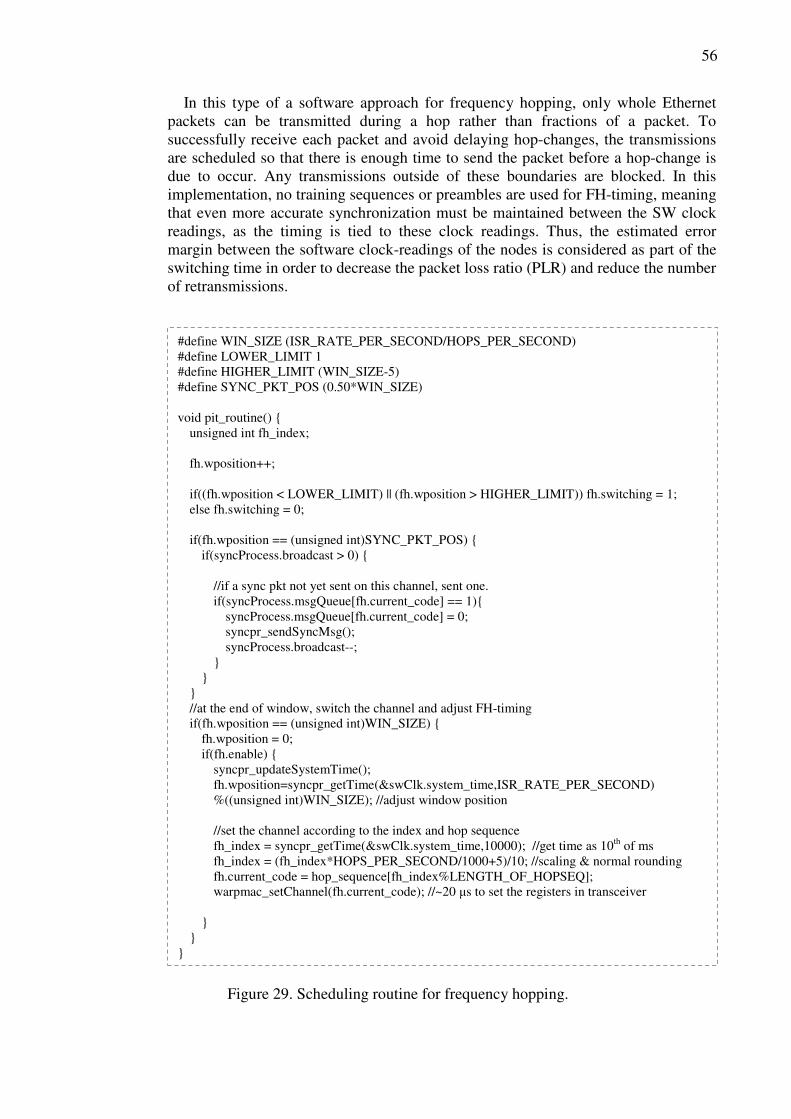
56

In this type of a software approach for frequency hopping, only whole Ethernet packets can be transmitted during a hop rather than fractions of a packet. To successfully receive each packet and avoid delaying hop-changes, the transmissions are scheduled so that there is enough time to send the packet before a hop-change is due to occur. Any transmissions outside of these boundaries are blocked. In this implementation, no training sequences or preambles are used for FH-timing, meaning that even more accurate synchronization must be maintained between the SW clock readings, as the timing is tied to these clock readings. Thus, the estimated error margin between the software clock-readings of the nodes is considered as part of the switching time in order to decrease the packet loss ratio (PLR) and reduce the number of retransmissions.

Figure 29. Scheduling routine for frequency hopping.

#define WIN_SIZE (ISR_RATE_PER_SECOND/HOPS_PER_SECOND) #define LOWER_LIMIT 1 #define HIGHER_LIMIT (WIN_SIZE-5) #define SYNC_PKT_POS (0.50*WIN_SIZE) void pit_routine() {

unsigned int fh_index; fh.wposition++; if((fh.wposition < LOWER_LIMIT) || (fh.wposition > HIGHER_LIMIT)) fh.switching = 1; else fh.switching = 0; if(fh.wposition == (unsigned int)SYNC_PKT_POS) {

if(syncProcess.broadcast > 0) {

//if a sync pkt not yet sent on this channel, sent one. if(syncProcess.msgQueue[fh.current_code] == 1){

syncProcess.msgQueue[fh.current_code] = 0; syncpr_sendSyncMsg(); syncProcess.broadcast--;

} }

} //at the end of window, switch the channel and adjust FH-timing if(fh.wposition == (unsigned int)WIN_SIZE) {

fh.wposition = 0; if(fh.enable) {

syncpr_updateSystemTime(); fh.wposition=syncpr_getTime(&swClk.system_time,ISR_RATE_PER_SECOND) %((unsigned int)WIN_SIZE); //adjust window position //set the channel according to the index and hop sequence fh_index = syncpr_getTime(&swClk.system_time,10000); //get time as 10th of ms fh_index = (fh_index*HOPS_PER_SECOND/1000+5)/10; //scaling & normal rounding fh.current_code = hop_sequence[fh_index%LENGTH_OF_HOPSEQ]; warpmac_setChannel(fh.current_code); //~20 µs to set the registers in transceiver

} }

}

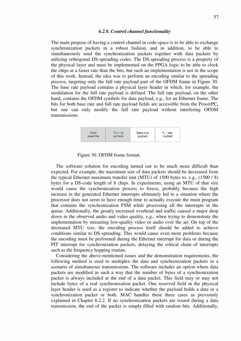
57

6.2.8. Control channel functionality The main purpose of having a control channel in code-space is to be able to exchange synchronization packets in a robust fashion, and in addition, to be able to simultaneously send the synchronization packets together with data packets by utilizing orthogonal DS-spreading codes. The DS-spreading process is a property of the physical layer and must be implemented on the FPGA logic to be able to clock the chips at a faster rate than the bits, but such an implementation is not in the scope of this work. Instead, the idea was to perform an encoding similar to the spreading process, targeting only the full rate payload part of the OFDM frame in Figure 30. The base rate payload contains a physical layer header in which, for example, the modulation for the full rate payload is defined. The full rate payload, on the other hand, contains the OFDM symbols for data payload, e.g., for an Ethernet frame. The bits for both base rate and full rate payload fields are accessible from the PowerPC, but one can only modify the full rate payload without interfering OFDM transmissions.

Figure 30. OFDM frame format.

The software solution for encoding turned out to be much more difficult than expected. For example, the maximum size of data packets should be decreased from the typical Ethernet maximum transfer unit (MTU) of 1500 bytes to, e.g., (1500 / 8) bytes for a DS-code length of 8 chips. In experiments, using an MTU of that size would cause the synchronization process to freeze, probably because the high increase in the generated Ethernet interrupts ultimately led to a situation where the processor does not seem to have enough time to actually execute the main program that contains the synchronization FSM while processing all the interrupts in the queue. Additionally, the greatly increased overhead and traffic caused a major drop down in the observed audio and video quality, e.g., when trying to demonstrate the implementation by streaming low-quality video or audio over the air. On top of the decreased MTU size, the encoding process itself should be added to achieve conditions similar to DS-spreading. This would cause even more problems because the encoding must be performed during the Ethernet interrupt for data or during the PIT interrupt for synchronization packets, delaying the critical chain of interrupts such as the frequency hopping routine. Considering the above-mentioned issues and the demonstration requirements, the following method is used to multiplex the data and synchronization packets in a scenario of simultaneous transmissions. The software includes an option where data packets are modified in such a way that the number of bytes of a synchronization packet is always included at the end of a data packet. This field may or may not include bytes of a real synchronization packet. One reserved field in the physical layer header is used as a register to indicate whether the payload holds a data or a synchronization packet or both. MAC handles these three cases as previously explained in Chapter 6.2.2. If no synchronization packets are issued during a data transmission, the end of the packet is simply filled with random bits. Additionally,

58

the same procedure can be used when sending a synchronization message so that the end of the packet is filled with random bits resulting in a packet with the same size in all cases, i.e., when streaming music or video over the air the size of the transmitted packets remains constant with or without synchronization information.

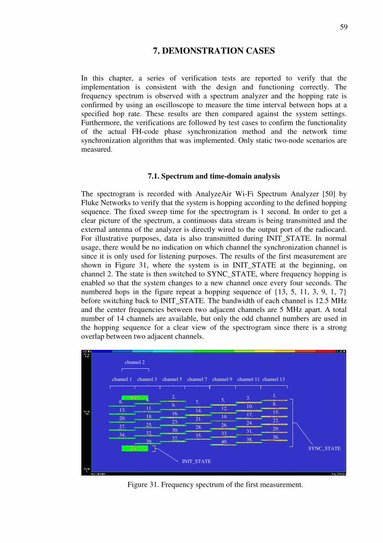
59

7. DEMONSTRATION CASES In this chapter, a series of verification tests are reported to verify that the implementation is consistent with the design and functioning correctly. The frequency spectrum is observed with a spectrum analyzer and the hopping rate is confirmed by using an oscilloscope to measure the time interval between hops at a specified hop rate. These results are then compared against the system settings. Furthermore, the verifications are followed by test cases to confirm the functionality of the actual FH-code phase synchronization method and the network time synchronization algorithm that was implemented. Only static two-node scenarios are measured.

7.1. Spectrum and time-domain analysis The spectrogram is recorded with AnalyzeAir Wi-Fi Spectrum Analyzer [50] by Fluke Networks to verify that the system is hopping according to the defined hopping sequence. The fixed sweep time for the spectrogram is 1 second. In order to get a clear picture of the spectrum, a continuous data stream is being transmitted and the external antenna of the analyzer is directly wired to the output port of the radiocard. For illustrative purposes, data is also transmitted during INIT_STATE. In normal usage, there would be no indication on which channel the synchronization channel is since it is only used for listening purposes. The results of the first measurement are shown in Figure 31, where the system is in INIT_STATE at the beginning, on channel 2. The state is then switched to SYNC_STATE, where frequency hopping is enabled so that the system changes to a new channel once every four seconds. The numbered hops in the figure repeat a hopping sequence of {13, 5, 11, 3, 9, 1, 7} before switching back to INIT_STATE. The bandwidth of each channel is 12.5 MHz and the center frequencies between two adjacent channels are 5 MHz apart. A total number of 14 channels are available, but only the odd channel numbers are used in the hopping sequence for a clear view of the spectrogram since there is a strong overlap between two adjacent channels.

Figure 31. Frequency spectrum of the first measurement.

1.

8.

15.

22.

29.

36.

3.

10.

17.

24.

31.

38.

5.

12.

19.

26.

33.

40.

7.

14.

21.

28.

35.

2.

9.

16.

23.

30.

37.

4.

11.

18.

25.

32.

39.

6.

13.

20.

27.

34.

INIT_STATE

SYNC_STATE

channel 1 channel 3 channel 5 channel 7 channel 9 channel 11 channel 13

channel 2

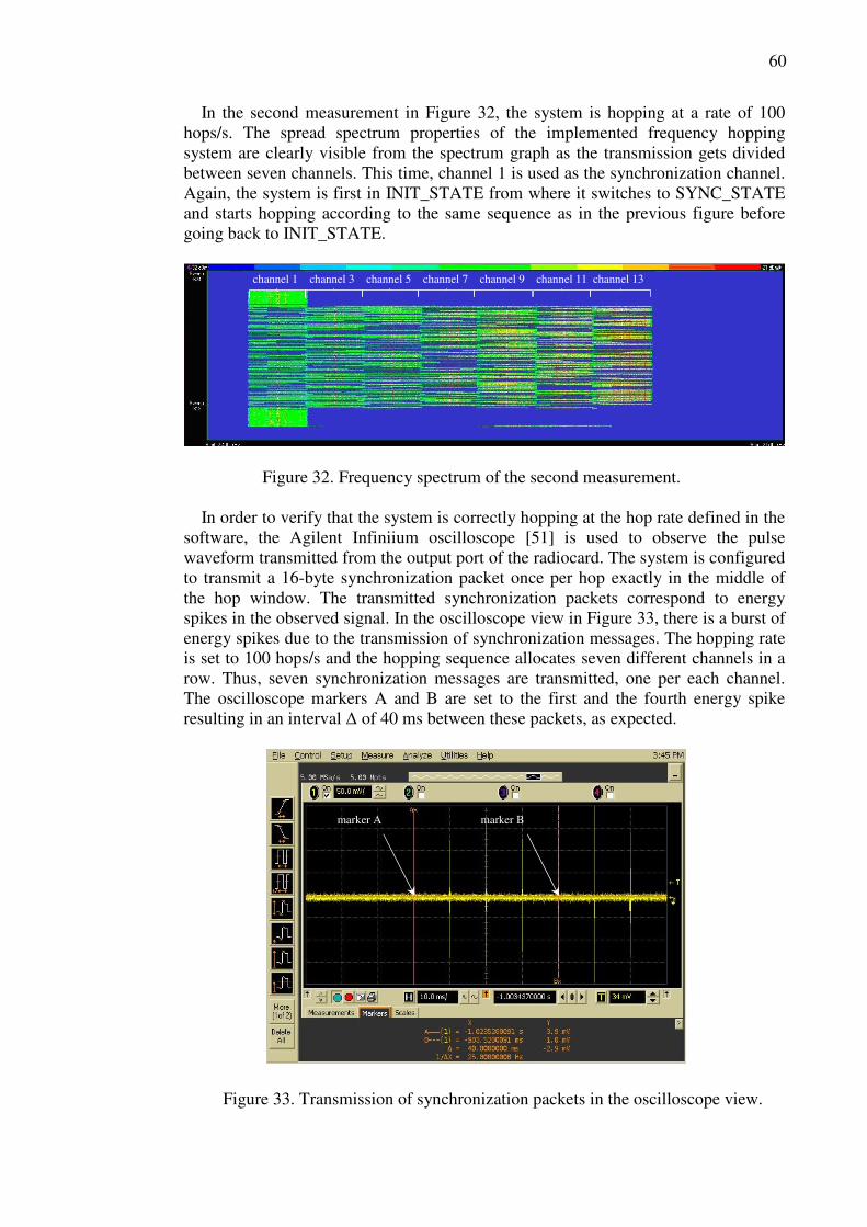
60

In the second measurement in Figure 32, the system is hopping at a rate of 100 hops/s. The spread spectrum properties of the implemented frequency hopping system are clearly visible from the spectrum graph as the transmission gets divided between seven channels. This time, channel 1 is used as the synchronization channel. Again, the system is first in INIT_STATE from where it switches to SYNC_STATE and starts hopping according to the same sequence as in the previous figure before going back to INIT_STATE.

Figure 32. Frequency spectrum of the second measurement. In order to verify that the system is correctly hopping at the hop rate defined in the software, the Agilent Infiniium oscilloscope [51] is used to observe the pulse waveform transmitted from the output port of the radiocard. The system is configured to transmit a 16-byte synchronization packet once per hop exactly in the middle of the hop window. The transmitted synchronization packets correspond to energy spikes in the observed signal. In the oscilloscope view in Figure 33, there is a burst of energy spikes due to the transmission of synchronization messages. The hopping rate is set to 100 hops/s and the hopping sequence allocates seven different channels in a row. Thus, seven synchronization messages are transmitted, one per each channel. The oscilloscope markers A and B are set to the first and the fourth energy spike resulting in an interval ∆ of 40 ms between these packets, as expected.

Figure 33. Transmission of synchronization packets in the oscilloscope view.

channel 1 channel 3 channel 5 channel 7 channel 9 channel 11 channel 13

marker A marker B

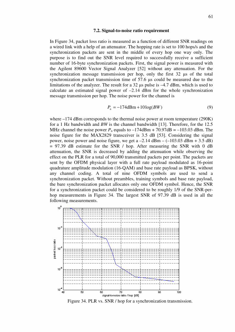
61

7.2. Signal-to-noise ratio requirement In Figure 34, packet loss ratio is measured as a function of different SNR readings on a wired link with a help of an attenuator. The hopping rate is set to 100 hops/s and the synchronization packets are sent in the middle of every hop one way only. The purpose is to find out the SNR level required to successfully receive a sufficient number of 16-byte synchronization packets. First, the signal power is measured with the Agilent 89600 Vector Signal Analyzer [52] without any attenuation. For the synchronization message transmission per hop, only the first 32 µs of the total synchronization packet transmission time of 57.6 µs could be measured due to the limitations of the analyzer. The result for a 32 µs pulse is –4.7 dBm, which is used to calculate an estimated signal power of –2.14 dBm for the whole synchronization message transmission per hop. The noise power for the channel is

)log(10dBm174n BWP +−= (9)

where –174 dBm corresponds to the thermal noise power at room temperature (290K) for a 1 Hz bandwidth and BW is the channel bandwidth [13]. Therefore, for the 12.5 MHz channel the noise power Pn equals to –174dBm + 70.97dB = –103.03 dBm. The noise figure for the MAX2829 transceiver is 3.5 dB [53]. Considering the signal power, noise power and noise figure, we get a –2.14 dBm – (–103.03 dBm + 3.5 dB) = 97.39 dB estimate for the SNR / hop. After measuring the SNR with 0 dB attenuation, the SNR is decreased by adding the attenuation while observing the effect on the PLR for a total of 90,000 transmitted packets per point. The packets are sent by the OFDM physical layer with a full rate payload modulated as 16-point quadrature amplitude modulation (16-QAM) and base rate payload as BPSK, without any channel coding. A total of nine OFDM symbols are used to send a synchronization packet. Without preambles, training symbols and base rate payload, the bare synchronization packet allocates only one OFDM symbol. Hence, the SNR for a synchronization packet could be considered to be roughly 1/9 of the SNR-per-hop measurements in Figure 34. The largest SNR of 97.39 dB is used in all the following measurements.

Figure 34. PLR vs. SNR / hop for a synchronization transmission.

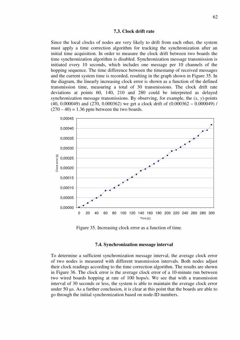
62

7.3. Clock drift rate Since the local clocks of nodes are very likely to drift from each other, the system must apply a time correction algorithm for tracking the synchronization after an initial time acquisition. In order to measure the clock drift between two boards the time synchronization algorithm is disabled. Synchronization message transmission is initiated every 10 seconds, which includes one message per 10 channels of the hopping sequence. The time difference between the timestamp of received messages and the current system time is recorded, resulting in the graph shown in Figure 35. In the diagram, the linearly increasing clock error is shown as a function of the defined transmission time, measuring a total of 30 transmissions. The clock drift rate deviations at points 60, 140, 210 and 280 could be interpreted as delayed synchronization message transmissions. By observing, for example, the (x, y)-points (40, 0.000049) and (270, 0.000362) we get a clock drift of (0.000362 – 0.000049) / (270 – 40) = 1.36 ppm between the two boards.

0,00000

0,00005

0,00010

0,00015

0,00020

0,00025

0,00030

0,00035

0,00040

0,00045

0 20 40 60 80 100 120 140 160 180 200 220 240 260 280 300Time [s]

Clo

ck e

rro

r [s

]

Figure 35. Increasing clock error as a function of time.

7.4. Synchronization message interval To determine a sufficient synchronization message interval, the average clock error of two nodes is measured with different transmission intervals. Both nodes adjust their clock readings according to the time correction algorithm. The results are shown in Figure 36. The clock error is the average clock error of a 10-minute run between two wired boards hopping at rate of 100 hops/s. We see that with a transmission interval of 30 seconds or less, the system is able to maintain the average clock error under 50 µs. As a further conclusion, it is clear at this point that the boards are able to go through the initial synchronization based on node-ID numbers.

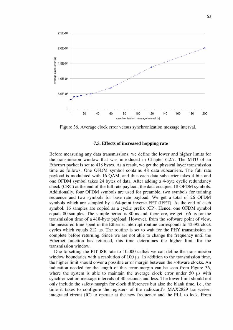
63

0

5.0E-05

1.0E-04

1.5E-04

2.0E-04

2.5E-04

1 20 40 60 80 100 120 140 160 180 200

synchronization message interval [s]

aver

age

cloc

k er

ror

[s]

Figure 36. Average clock error versus synchronization message interval.

7.5. Effects of increased hopping rate Before measuring any data transmissions, we define the lower and higher limits for the transmission window that was introduced in Chapter 6.2.7. The MTU of an Ethernet packet is set to 418 bytes. As a result, we get the physical layer transmission time as follows. One OFDM symbol contains 48 data subcarriers. The full rate payload is modulated with 16-QAM, and thus each data subcarrier takes 4 bits and one OFDM symbol takes 24 bytes of data. After adding a 4-byte cyclic redundancy check (CRC) at the end of the full rate payload, the data occupies 18 OFDM symbols. Additionally, four OFDM symbols are used for preamble, two symbols for training sequence and two symbols for base rate payload. We get a total of 26 OFDM symbols which are sampled by a 64-point inverse FFT (IFFT). At the end of each symbol, 16 samples are copied as a cyclic prefix (CP). Hence, one OFDM symbol equals 80 samples. The sample period is 80 ns and, therefore, we get 166 µs for the transmission time of a 418-byte payload. However, from the software point of view, the measured time spent in the Ethernet interrupt routine corresponds to 42392 clock cycles which equals 212 µs. The routine is set to wait for the PHY transmission to complete before returning. Since we are not able to change the frequency until the Ethernet function has returned, this time determines the higher limit for the transmission window. Due to setting the PIT ISR rate to 10,000 calls/s we can define the transmission window boundaries with a resolution of 100 µs. In addition to the transmission time, the higher limit should cover a possible error margin between the software clocks. An indication needed for the length of this error margin can be seen from Figure 36, where the system is able to maintain the average clock error under 50 µs with synchronization message intervals of 30 seconds and less. The lower limit should not only include the safety margin for clock differences but also the blank time, i.e., the time it takes to configure the registers of the radiocard’s MAX2829 transceiver integrated circuit (IC) to operate at the new frequency and the PLL to lock. From

64

Figure 37 [53], it can be seen that the time for a frequency to settle when switched from 2500 MHz to 2400 MHz is approximately 37 µs. Therefore, we set the lower limit for the transmission window to 100 µs for the upcoming measurements with data stream, which covers the sum of the previous times (uncertainty of clocks and blank time). With this information, we can also calculate the theoretical maximum hop rate for the implemented software with the given transmission window boundaries. The maximum rate directly depends on the MTU of the Ethernet packet. For example, for the 418-byte packet we need a lower limit of 100 µs and a higher limit of 300 µs, i.e., there would be only one position along the hop window to transmit a packet. Consequently, we get a maximum hop rate of 2500 hops/s for the implementation which can be further increased by decreasing the maximum Ethernet packet size and the higher limit needed to transmit the packet. Nevertheless, it should be noted that rates above 1000 hops/s require a slight modification of the FH-scheduling routine in the current implementation. Therefore, we only use hopping rates up to 1000 hops/s for the upcoming measurements.

Figure 37. Channel switching frequency deviation for MAX2829 transceiver IC.

There are two scenarios in Figure 38. Both times we stream user datagram protocol (UDP) packets that have an MTU of 418 bytes, which was also used in the previous examples. To eliminate the unknown factors of the radio channel, a wired link is used to connect the two boards instead of the wireless link. The packet loss ratio is observed as a function of hopping rate after 60,000 transmitted packets. These packets are sent in arbitrary transmission window positions while being generated from the Ethernet interface. The synchronization process is transmitting a 16-byte packet on each 10 channels of the hopping sequence, once every 10 seconds. For simplicity, the control channel functionality is not used, i.e., the data and synchronization packets are not multiplexed in any situations, and the normal MAC operations for data transmissions such as timeouts and ACK messages are disabled. As a result, only one-way traffic is present. Initially, for a non-hopping scenario a PLR of 0.0058 is measured. The first series in the Figure 38 graph represents the packet loss ratio when the hopping rate is increased with a higher limit of 200 µs for the transmission window. It is clearly visible from the graph that 200 µs does not suffice since the PLR strongly increases with the increasing hopping rate. In the second series, the higher limit is now 300 µs. We observe that the PLR stays approximately constant throughout the various hopping rates once a sufficient higher limit has been set for the transmission window. However, the increased hop rate

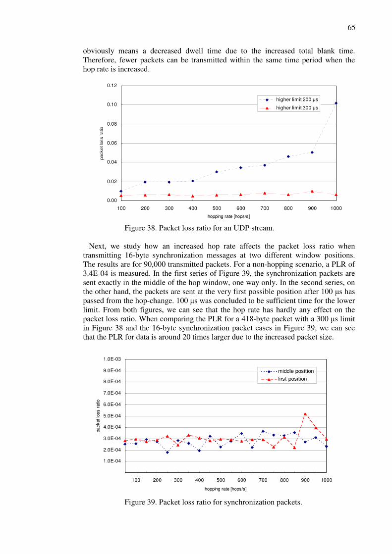
65

obviously means a decreased dwell time due to the increased total blank time. Therefore, fewer packets can be transmitted within the same time period when the hop rate is increased.

0.00

0.02

0.04

0.06

0.08

0.10

0.12

100 200 300 400 500 600 700 800 900 1000

hopping rate [hops/s]

pack

et lo

ss r

atio

higher limit 200 µs

higher limit 300 µs

Figure 38. Packet loss ratio for an UDP stream. Next, we study how an increased hop rate affects the packet loss ratio when transmitting 16-byte synchronization messages at two different window positions. The results are for 90,000 transmitted packets. For a non-hopping scenario, a PLR of 3.4E-04 is measured. In the first series of Figure 39, the synchronization packets are sent exactly in the middle of the hop window, one way only. In the second series, on the other hand, the packets are sent at the very first possible position after 100 µs has passed from the hop-change. 100 µs was concluded to be sufficient time for the lower limit. From both figures, we can see that the hop rate has hardly any effect on the packet loss ratio. When comparing the PLR for a 418-byte packet with a 300 µs limit in Figure 38 and the 16-byte synchronization packet cases in Figure 39, we can see that the PLR for data is around 20 times larger due to the increased packet size.

1.0E-04

2.0E-04

3.0E-04

4.0E-04

5.0E-04

6.0E-04

7.0E-04

8.0E-04

9.0E-04

1.0E-03

100 200 300 400 500 600 700 800 900 1000

hopping rate [hops/s]

pack

et lo

ss r

atio

middle position

first position

Figure 39. Packet loss ratio for synchronization packets.

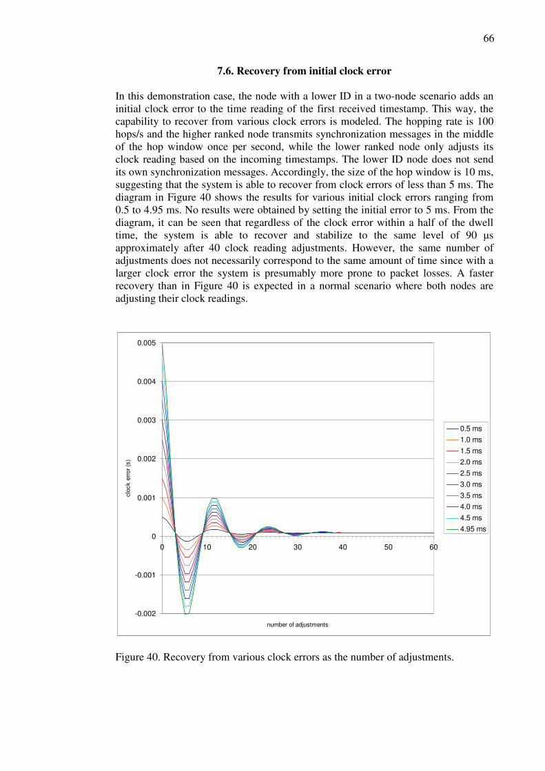
66

7.6. Recovery from initial clock error In this demonstration case, the node with a lower ID in a two-node scenario adds an initial clock error to the time reading of the first received timestamp. This way, the capability to recover from various clock errors is modeled. The hopping rate is 100 hops/s and the higher ranked node transmits synchronization messages in the middle of the hop window once per second, while the lower ranked node only adjusts its clock reading based on the incoming timestamps. The lower ID node does not send its own synchronization messages. Accordingly, the size of the hop window is 10 ms, suggesting that the system is able to recover from clock errors of less than 5 ms. The diagram in Figure 40 shows the results for various initial clock errors ranging from 0.5 to 4.95 ms. No results were obtained by setting the initial error to 5 ms. From the diagram, it can be seen that regardless of the clock error within a half of the dwell time, the system is able to recover and stabilize to the same level of 90 µs approximately after 40 clock reading adjustments. However, the same number of adjustments does not necessarily correspond to the same amount of time since with a larger clock error the system is presumably more prone to packet losses. A faster recovery than in Figure 40 is expected in a normal scenario where both nodes are adjusting their clock readings.

-0.002

-0.001

0

0.001

0.002

0.003

0.004

0.005

0 10 20 30 40 50 60

number of adjustments

cloc

k er

ror

(s)

0.5 ms

1.0 ms

1.5 ms

2.0 ms

2.5 ms

3.0 ms

3.5 ms

4.0 ms

4.5 ms

4.95 ms

Figure 40. Recovery from various clock errors as the number of adjustments.

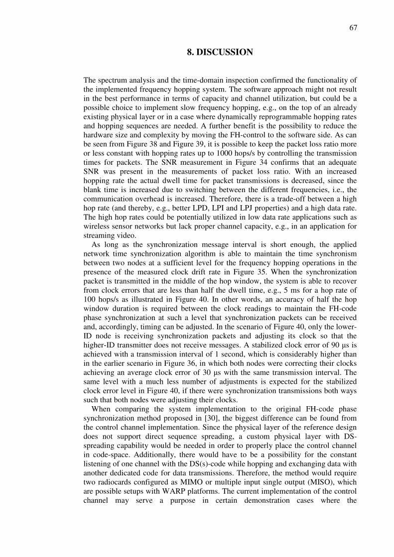
67

8. DISCUSSION The spectrum analysis and the time-domain inspection confirmed the functionality of the implemented frequency hopping system. The software approach might not result in the best performance in terms of capacity and channel utilization, but could be a possible choice to implement slow frequency hopping, e.g., on the top of an already existing physical layer or in a case where dynamically reprogrammable hopping rates and hopping sequences are needed. A further benefit is the possibility to reduce the hardware size and complexity by moving the FH-control to the software side. As can be seen from Figure 38 and Figure 39, it is possible to keep the packet loss ratio more or less constant with hopping rates up to 1000 hops/s by controlling the transmission times for packets. The SNR measurement in Figure 34 confirms that an adequate SNR was present in the measurements of packet loss ratio. With an increased hopping rate the actual dwell time for packet transmissions is decreased, since the blank time is increased due to switching between the different frequencies, i.e., the communication overhead is increased. Therefore, there is a trade-off between a high hop rate (and thereby, e.g., better LPD, LPI and LPJ properties) and a high data rate. The high hop rates could be potentially utilized in low data rate applications such as wireless sensor networks but lack proper channel capacity, e.g., in an application for streaming video. As long as the synchronization message interval is short enough, the applied network time synchronization algorithm is able to maintain the time synchronism between two nodes at a sufficient level for the frequency hopping operations in the presence of the measured clock drift rate in Figure 35. When the synchronization packet is transmitted in the middle of the hop window, the system is able to recover from clock errors that are less than half the dwell time, e.g., 5 ms for a hop rate of 100 hops/s as illustrated in Figure 40. In other words, an accuracy of half the hop window duration is required between the clock readings to maintain the FH-code phase synchronization at such a level that synchronization packets can be received and, accordingly, timing can be adjusted. In the scenario of Figure 40, only the lower-ID node is receiving synchronization packets and adjusting its clock so that the higher-ID transmitter does not receive messages. A stabilized clock error of 90 µs is achieved with a transmission interval of 1 second, which is considerably higher than in the earlier scenario in Figure 36, in which both nodes were correcting their clocks achieving an average clock error of 30 µs with the same transmission interval. The same level with a much less number of adjustments is expected for the stabilized clock error level in Figure 40, if there were synchronization transmissions both ways such that both nodes were adjusting their clocks. When comparing the system implementation to the original FH-code phase synchronization method proposed in [30], the biggest difference can be found from the control channel implementation. Since the physical layer of the reference design does not support direct sequence spreading, a custom physical layer with DS-spreading capability would be needed in order to properly place the control channel in code-space. Additionally, there would have to be a possibility for the constant listening of one channel with the DS(s)-code while hopping and exchanging data with another dedicated code for data transmissions. Therefore, the method would require two radiocards configured as MIMO or multiple input single output (MISO), which are possible setups with WARP platforms. The current implementation of the control channel may serve a purpose in certain demonstration cases where the

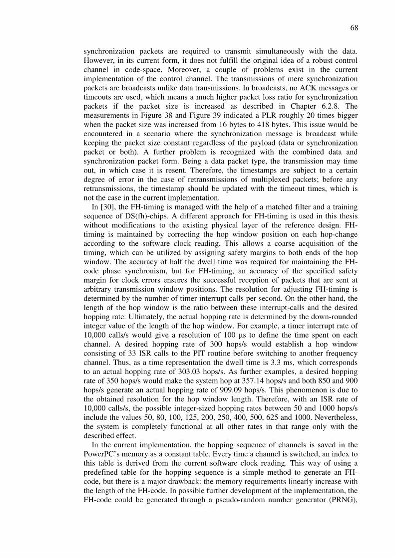
68

synchronization packets are required to transmit simultaneously with the data. However, in its current form, it does not fulfill the original idea of a robust control channel in code-space. Moreover, a couple of problems exist in the current implementation of the control channel. The transmissions of mere synchronization packets are broadcasts unlike data transmissions. In broadcasts, no ACK messages or timeouts are used, which means a much higher packet loss ratio for synchronization packets if the packet size is increased as described in Chapter 6.2.8. The measurements in Figure 38 and Figure 39 indicated a PLR roughly 20 times bigger when the packet size was increased from 16 bytes to 418 bytes. This issue would be encountered in a scenario where the synchronization message is broadcast while keeping the packet size constant regardless of the payload (data or synchronization packet or both). A further problem is recognized with the combined data and synchronization packet form. Being a data packet type, the transmission may time out, in which case it is resent. Therefore, the timestamps are subject to a certain degree of error in the case of retransmissions of multiplexed packets; before any retransmissions, the timestamp should be updated with the timeout times, which is not the case in the current implementation. In [30], the FH-timing is managed with the help of a matched filter and a training sequence of DS(fh)-chips. A different approach for FH-timing is used in this thesis without modifications to the existing physical layer of the reference design. FH-timing is maintained by correcting the hop window position on each hop-change according to the software clock reading. This allows a coarse acquisition of the timing, which can be utilized by assigning safety margins to both ends of the hop window. The accuracy of half the dwell time was required for maintaining the FH-code phase synchronism, but for FH-timing, an accuracy of the specified safety margin for clock errors ensures the successful reception of packets that are sent at arbitrary transmission window positions. The resolution for adjusting FH-timing is determined by the number of timer interrupt calls per second. On the other hand, the length of the hop window is the ratio between these interrupt-calls and the desired hopping rate. Ultimately, the actual hopping rate is determined by the down-rounded integer value of the length of the hop window. For example, a timer interrupt rate of 10,000 calls/s would give a resolution of 100 µs to define the time spent on each channel. A desired hopping rate of 300 hops/s would establish a hop window consisting of 33 ISR calls to the PIT routine before switching to another frequency channel. Thus, as a time representation the dwell time is 3.3 ms, which corresponds to an actual hopping rate of 303.03 hops/s. As further examples, a desired hopping rate of 350 hops/s would make the system hop at 357.14 hops/s and both 850 and 900 hops/s generate an actual hopping rate of 909.09 hops/s. This phenomenon is due to the obtained resolution for the hop window length. Therefore, with an ISR rate of 10,000 calls/s, the possible integer-sized hopping rates between 50 and 1000 hops/s include the values 50, 80, 100, 125, 200, 250, 400, 500, 625 and 1000. Nevertheless, the system is completely functional at all other rates in that range only with the described effect. In the current implementation, the hopping sequence of channels is saved in the PowerPC’s memory as a constant table. Every time a channel is switched, an index to this table is derived from the current software clock reading. This way of using a predefined table for the hopping sequence is a simple method to generate an FH-code, but there is a major drawback: the memory requirements linearly increase with the length of the FH-code. In possible further development of the implementation, the FH-code could be generated through a pseudo-random number generator (PRNG),

69

e.g., by utilizing the FH-index that was introduced in Chapter 6.2.7. This index of the FH-scheduling process increments by 1 on each frequency hop. Since the FH-index is derived from the 64-bit software clock reading, it accordingly rolls over about every 3000 years with the 200 MHz system clock. In a time-synchronized network, the FH-index is equivalent for all nodes as long as there is no time difference of more than half of the dwell time between the nodes. Therefore, rather than spending the memory resources on saving the individual channel numbers of the hopping sequence, this index could be used as a seed value for a PRNG-algorithm to generate a very long FH-code. As a further development, the OFDM physical layer could be modified to support DS-spreading in order to form a control channel with two orthogonal codes, as originally proposed in [30]. Additionally, further improvements could be made by optimizing all the parameters regarding frequency hopping and time synchronization. For example, experiments could be carried out with a higher PIT rate for a better FH-timing resolution. The maximum clock error between the nodes of the network ultimately determines a rational resolution for FH-timing. The resolution, on the other hand, directly defines the required size of the timestamp. Currently, the used 64-bit timestamp with a precision down to 5 ns is excessive since only a precision of 0.1 ms of the timestamp is utilized in both FH-timing and determining the FH-code phase. However, the minimum full rate payload to transmit is 24 bytes with 16-QAM, i.e., one OFDM symbol. Thus, the optimal size for a synchronization packet is 20 bytes, to which the system adds a 4-byte CRC check. Therefore, there is no benefit in cutting down the size of a synchronization packet or the timestamp with the current OFDM physical layer. All the measurements and results in this thesis were from a static two-node scenario. Experiments with three and more boards are considered in future test cases. The objectives of this work were two-fold: first, to implement frequency hopping capability on top of an existing physical layer and, second, to implement and demonstrate a frequency hopping code phase synchronization method. Both of these goals were met so that the frequency hopping ad hoc nodes are able to synchronize with each other and form a network. The synchronism is maintained with the help of a discrete network synchronization algorithm. However, for a full-scale implementation of the chosen synchronization method, a custom physical layer would have been required. Therefore, this implementation is only partially consistent with the original method proposed in [30].

70

9. SUMMARY A secure ad hoc network requires good LPJ, LPI and LPD capabilities. A network fulfilling these requirements can be established by using spread spectrum techniques such as frequency hopping. Synchronizing an FH ad hoc network can be problematic and must be carefully designed. Without having any centralized control the nodes in an ad hoc network must make a distributed decision about the common FH-code phase. Additionally, the whole synchronization procedure should remain invisible to any outsiders but still allow all the intended users to exchange synchronization information with different FH-code phase offsets. If the FH-code phase is directly derived from the local clock readings of each node, it is essential to achieve network-wide time synchronization for an effectively operating frequency hopping ad hoc network. In this thesis, the issues of synchronizing a frequency hopping ad hoc network were studied. One of the FH-code phase synchronization methods was described in detail and implemented on research platforms. The studied synchronization method forms a control channel in code-space by using DS-spreading. Simultaneous transmission of data and synchronization information is possible due to using orthogonal spreading codes. When the synchronization transmission is issued, the synchronization message is sent on each frequency channel allocated for the hopping sequence. This way the receiver can arbitrarily select a synchronization channel to listen to and avoid any occupied frequency channels providing excellent protection against intentional jamming. Two different training sequences are used for matched filters to acquire the DS-code phase and FH-timing so that the hop-changes occur at the right time instant at both ends. At the initial stage, a hierarchy based on node-ID numbers is used to determine whose local clock reading is chosen as the common time reference for the network. Thereafter, a discrete network synchronization algorithm is applied to adjust the clock reading according to the time information of synchronization packets. The FH-code phase synchronization method was implemented on the WARP. WARP boards are designed by Rice University for research and educational purposes to prototype wireless networks. The boards are using an FPGA device with embedded PowerPC processors and FPGA logic allowing both physical and network layer implementations on a single platform. In this work, a software approach was presented on the PowerPC for establishing, managing and synchronizing a frequency hopping ad hoc network above a provided OFDM physical layer. The implementation of the frequency hopping functionality contains a specific routine which utilizes a radio controller command to set a new center frequency according to the current clock reading and the predefined hopping sequence. Instead of using a training sequence and a matched filter as proposed for the original method, only a coarse acquisition of the FH-timing is obtained by deriving the timing from the software clock reading. The clock uncertainties are accommodated by defining safety margins at both ends of the hop window. These safety margins assure that no packet transmissions are attempted outside of the boundaries, e.g., when the other node has already changed its frequency. In addition, the blank time for the transceiver to switch to the new frequency is considered and a deadline is set for transmissions blocking any attempts of MAC to forward packets when there is an insufficient amount of dwell time left for the physical layer to transmit a packet. The desired MTU of an Ethernet packet was concluded to mainly determine the maximum

71

hopping rate. The achieved system is slow frequency hopping since multiple OFDM symbols are transmitted per hop. Although the topic is a synchronization method aimed at the MANET category of networks where energy constraints are usually very important, this aspect was not considered in this implementation. In the experiments for a static two-node scenario, the boards made a distributed decision about the common FH-code phase based on the node-ID numbers. The discrete network synchronization algorithm was able to maintain time synchronism at a sufficient level for the frequency hopping operations as long as the synchronization message interval is short enough to compensate for the clock drift rate between the boards. Measurements indicated that clock errors of less than half the hop window duration are required between the nodes to keep the synchronization process functioning and maintain the FH-code phase synchronism between the nodes. The hop window position at which a packet is sent was concluded not to affect the packet loss ratio as long as there is a sufficient distance from the edges of the hop. The necessity of limiting transmission times was demonstrated with data transmission. The packet loss ratio increases with the hopping rate if there is not enough time for the physical layer to transmit the packet. In a properly controlled scenario, the increased hopping rate had hardly any effect on the functionality of the system except for the decreased dwell time, resulting in lower data rates. Consequently, a trade-off was recognized between a high data rate and a high hopping rate. The implemented FH-code phase synchronization method is only partially consistent with the original method. A custom physical layer implementation with DS-spreading capability would have been required to be able to place the control channel in code-space. Furthermore, two radio cards for each WARP would be needed in order to constantly listen to one channel for DS(s)-coded synchronization information while hopping according to the hopping pattern and to exchange data packets with another DS-code. Currently, the implemented control channel is able to simultaneously transmit synchronization information and data packets but lacks the desired robustness. Therefore, possible further development of the implementation primarily concerns the issues of the control channel. Moreover, FH-code generation could be pseudo-randomized and additional improvements could be made by optimizing all the parameters regarding the frequency hopping functionality and the synchronization state machine.

72

10. REFERENCES

[1] Akyildiz I. F., Su W., Sankarasubramaniam Y. & Cayirci E. (2002) Wireless Sensor Networks: a Survey. The International Journal of Computer and Telecommunications Networking, Vol. 38, No. 4 (March), p. 393-422.

[2] Karl W. & Willig A. (2005) Protocols and Architectures for Wireless Sensor Networks. John Wiley & Sons Ltd, 481 p.

[3] Dressler F. (2006) Self-Organization in Ad Hoc Networks: Overview and Classifications. Technical Report 02/06. University Of Erlangen, Department of Computer Science 7, Erlangen, Germany.

[4] Culler D., Srivastava M. & Estrin D. (2004) Guest Editors’ Introduction: Overview of Sensor Networks. IEEE Computer, Vol. 37, No. 8 (August), p. 41–49.

[5] Santi P. (2005) Topology Control in Wireless Ad Hoc and Sensor Networks. ACM Computing Surveys (CSUR), Vol. 37, No. 2 (June), p. 164-194.

[6] Wattenhofer R., Li L., Bahl P. & Wang Y.-M., (2001) Distributed Topology Control for Power Efficient Operation in Multihop Wireless Ad Hoc Networks. In: Proceedings of the Conference of IEEE Computer and Communications Societies (INFOCOM), April 22 – 26, Anchorage, Alaska, p. 1388-1397.

[7] Kumar S., Raghavan V. S. & Deng J. (2006) Medium Access Control Protocols for Ad Hoc Wireless Networks: A Survey. Elsevier Ad Hoc Networks Journal, Vol. 4, No. 3, p. 326-358.

[8] Pahlavan K. (2002) Principles of Wireless Networks: A Unified Approach. Prentice Hall Professional Technical Reference, 608 p.

[9] Tobagi F. A. (1980) Multiaccess Protocols in Packet Communication Systems. IEEE Transactions on Communications, Vol. COM-28, No. 4 (April), p. 468-488.

[10] Tanenbaum A. S. (2003) Computer Networks, Fourth Edition. Prentice Hall Professional Technical Reference, 869 p.

[11] Jayasuriya A., Perreau S., Dadej A. & S. Gordon (2004) Hidden vs. Exposed Terminal Problem in Ad hoc Networks. In: Proceedings of the Australian Telecommunication Networks and Applications Conference (ATNAC), December 8 – 10, Sydney, Australia, p. 52-59.

[12] Brenner P. (1997) A Technical Tutorial on the IEEE 802.11 Protocol. URL: http://www.sss-mag.com/pdf/802_11tut.pdf.

[13] Proakis J.G. (2001) Digital Communications, Fourth Edition. McGraw-Hill Companies, 993 p.

73

[14] Tang C. Y., Yi Y. & Freebersyser J. A. (2007) Media Access Control Protocol

for Mobile Ad Hoc Networks Using CDMA and Multiuser Detection. Honeywell Laboratories, Minneapolis, USA. Draft available at: http://faculty-staff.ou.edu/T/Choon.Yik.Tang-1/.

[15] Kohno R., Meidan R. & Milstein L. B. (1995) Spread Spectrum Access Methods for Wireless Communications. IEEE Communications Magazine (January), p. 58-67.

[16] Prokkola J. & Bräysy T. (2004) Bi-Code Channel Access Method for Ad Hoc Networks. In: Proceedings of the 8th IEEE International Symposium on Spread Spectrum Techniques and Applications (ISSSTA2004), August 30 – September 2, Sydney, Australia, p. 232-236.

[17] Prokkola J. & Bräysy T. (2004) Bi-Code Channel Access with Robust Medium Access Control for Ad Hoc Networking. Military Communication Conference (MILCOM 2004), October 31 – November 3, Monterey, USA, p. 1-7.

[18] Johnson D.B. & Maltz D.A. (1996) Dynamic Source Routing in Wireless Ad Hoc Networks. In: Imielinski T. & Korth H. (Eds.), Mobile Computing, Kluwer Academic, Dordrecht, p. 153-179 (Chapter 5).

[19] Larsson T. & Hedman N. (1998) Routing Protocols in Wireless Ad-hoc Networks – Simulation Study. Master’s Thesis. Luleå University of Technology.

[20] Royer E. & Toh C-K. (1999) A Review of Current Routing Protocols for Ad-Hoc Mobile Wireless Networks. IEEE Personal Communications (April), p. 46-55.

[21] Frikha M. & Maamer M. (2006) Implementation and Simulation of OLSR Protocol With QoS in Ad Hoc Networks. IEEE International Symposium on Communications, Control, and Signal Processing (ISCCSP'06), March 13 - 15, Marrakech, Maroc.

[22] Sundararaman B., Buy U. & Kshemkalyani A.D. (2005) Clock Synchronization For Wireless Sensor Networks: A Survey. Elsevier Ad Hoc Networks, Vol. 3, No. 3 (May), p. 281–323.

[23] Römer K. (2001) Time Synchronization in Ad Hoc Networks. International Symposium on Mobile Ad Hoc Networking & Computing. In: Proceedings of the 2nd ACM International Symposium on Mobile Ad Hoc Networking & Computing (MobiHoc’01), October 4 - 5, Long Beach, CA, USA, p. 173-182.

[24] Windl U., Dalton D., Martinec M. & Worley D. R. (2006) The NTP FAQ and HOWTO: Understanding and using the Network Time Protocol, 3.3 Clock Quality. URL: http://www.ntp.org/ntpfaq/.

74

[25] Römer K., Blum P. & Meier L. (2005) Time Synchronization and Calibration in

Wireless Sensor Networks. In: Ivan Stojmenovic (Ed.): Handbook of Sensor Networks: Algorithms and Architectures. John Wiley & Sons, p.199-237.

[26] Elson J. & Römer K. (2003) Wireless Sensor Networks: A New Regime for Time Synchronization. ACM Computer Communication Review (CCR), Vol. 33, No. 1 (January), p. 149–154.

[27] Anceaume E. & Puaut I. (1997) A Taxonomy of Clock Synchronization Algorithms. Research Report. IRISA, Campus Universitaire de Beaulieu, Rennes Cedex, France, 25 p.

[28] Elson J., Girod L. & Estrin D. (2002) Fine-grained Network Time Synchronization Using Reference Broadcasts. In: Proceedings of the Fifth Symposium on Operating Systems Design and Implementation (OSDI’02), Vol. 36, Issue SI (Winter), p. 147–163.

[29] Greunen J.V. & Rabaey J. (2003) Lightweight Time Synchronization for Sensor Networks. In: Proceedings of the 2nd ACM International Conference on Wireless Sensor Networks and Applications (WSNA), September 19, San Diego, CA, USA, p. 11-19.

[30] Vanninen T., Saarnisaari H., Raustia M. & Koskela T. (2006) FH-code Phase Synchronization in a Wireless Multi-hop FH/DSSS Adhoc Network. In: Proceedings of Military Communication Conference (MILCOM’06), October 23 - 25, Washington DC, USA, p. 1-7.

[31] Saarnisaari H. (2005) Analysis of a Discrete Network Synchronization Algorithm. In: Proceedings of Military Communications Conference (MILCOM’05), October 17 - 20, Atlantic City, NJ, USA, Vol. 2, p. 740-746.

[32] A. Davies (1975) Discrete-Time Synchronization of Digital Data Networks. IEEE Transactions on Circuits and Systems, Vol. 22, No. 7 (July), p. 610–618.

[33] Torrieri D. J. (2000) Mobile Frequency-Hopping CDMA Systems. IEEE Transactions on Communications, Vol. 48, No. 8 (August), p. 1318-1327.

[34] Glas J. (1996) Non-Cellular Wireless Communication Systems. PhD thesis. Delft University of Technology. URL: http://cas.et.tudelft.nl/~glas/thesis.

[35] Glomie N., Chevrollier N. & Rebala, O. (2003) Bluetooth and WLAN Coexistence: Challenges and Solutions. IEEE Wireless Communications, Vol. 10, No. 6 (December), p. 22-29.

[36] Hassan A., Hershey J. & Saulnier G. (1998) Perspectives in Spread Spectrum. Kluwer Academic Publishers, 163 p.

[37] ShreHarsha R. (2005) Make the Most of Unlicensed ISM Bands. Wireless Net DesignLine. URL: http://www.wirelessnetdesignline.com/.

75

[38] Peterson B. (2004) Device Discovery in Frequency Hopping Wireless Ad Hoc

Networks. Doctorial thesis. Air Force Institute of Technology, Wright-Patterson Air Force Base, Ohio, USA.

[39] Lansford J. & Bahl P. (2000) The Design and Implementation of HomeRF: A Radio Frequency Wireless Networking Standard for the Connected Home. In: Proceedings of the IEEE, Vol. 88, No. 10, p. 1662-1676.

[40] Zyren J., Godfrey T. & Eaton D. (2001) Does Frequency Hopping Enhance Security? URL: http://www.packetnexus.com/docs/.

[41] Salonidis T., Bhagwat P., Tassiulas L. & LaMaire R. (2005) Distributed Topology Construction of Bluetooth Wireless Personal Area Networks. IEEE Journal on Selected Areas in Communications, Vol. 23, No. 3 (March), p. 633-643.

[42] Juntti M., Latva-aho M., Kansanen K. & Kaurahalme O-P. (1998) Performance of Parallel Interference Cancellation for CDMA in Estimated Fading Channels with Delay Mismatch. In: IEEE Proceedings of International Symposium on Spread Spectrum Techniques and Applications, September 2-4, Sun City, South Africa, Vol. 3, p. 936-940.

[43] WARP website (28.4.2008) URL: http://warp.rice.edu.

[44] Murphy P., Sabharwal A. & Aazhang B. (2006) Design of WARP: A Wireless Open-Access Research Platform. In: Proceedings of the 14th European Signal Processing Conference (EUSIPCO).

[45] Hamblen J. (28.4.2008) Embedded Processor Design project slides. URL: http://users.ece.gatech.edu/~hamblen/4006/xup/embedded/slides/03_hardware_ design.ppt.

[46] PowerPC Processor Reference Guide (2007) UG011 (v1.2) January 19. URL: www.xilinx.com/ise/embedded/edk92i_docs/ppc_ref_guide.pdf.

[47] Amiri K., Sun Y., Murphy P., Hunter C., Cavallaro J. & Sabharwal A. (2007) WARP, a Modular Testbed for Configurable Wireless Network Research at Rice. In: Proceedings of IEEE SWRIF, Houston, TX, May 2007.

[48] Hunter C., Camp J., Murphy P., Sabharwal A. & Dick C. (2006) A Flexible Framework for Wireless Medium Access Protocols. In: Proceedings of Asilomar Conference on Signals, Systems and Computers (ACSSC '06), October 29 – November 1, California, USA, p. 2046-2050.

[49] Xilkernel Embedded Development Kit 9.1i documentation (2006) URL: http://www.xilinx.com/ise/embedded/edk91i_docs/xilkernel_v3_00_a.pdf.

[50] AnalyzeAir Wi-Fi Spectrum Analyzer Users Manual (13.5.2008) URL: http://www.flukenetworks.com/FNet/en-us/findit?Document=9821679.

76

[51] Service Guide for Agilent Model 80000 Series Infiniium Oscilloscopes (2005)

URL: http://cp.literature.agilent.com/litweb/pdf/54856-97001.pdf.

[52] Technical Overview of Agilent 89600 Series Vector Signal Analyzer (2007) URL: http://cp.literature.agilent.com/litweb/pdf/5989-1679EN.pdf.

[53] MAX2828/MAX2829 Transceiver IC Datasheet document (2004) Available per request at: http://www.maxim-ic.com.

77

11. APPENDIXES Appendix 1. Timing diagram for FH-scheduling routine.

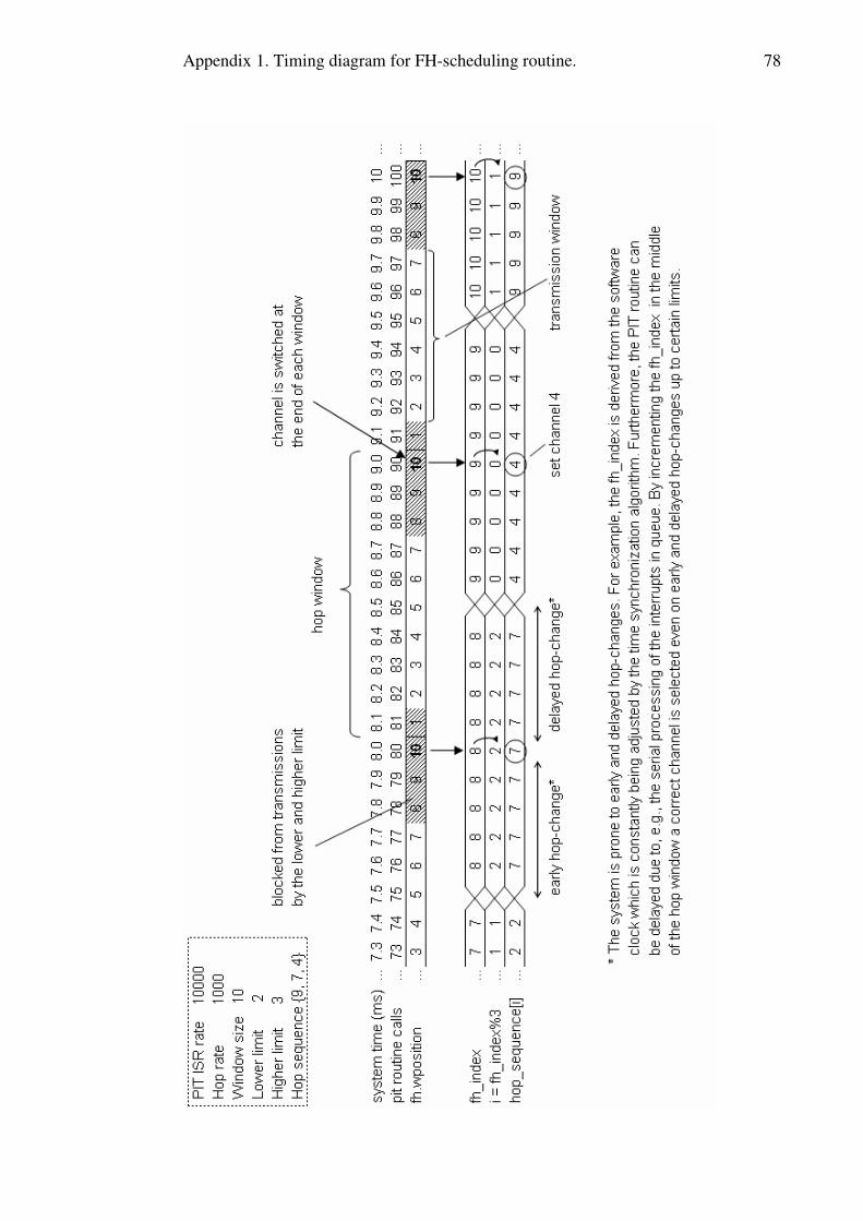
Appendix 1. Timing diagram for FH-scheduling routine. 78