Embed Size (px)
Citation preview

Sudan University of Science and Technology
College of Graduate Studies
School of Electronics Engineering
Implementing Nayan Seth’s Dynamic Load Balancing
Algorithm in Software-Defined Networks: A case study
الديناميكية في الشبكات المعرفة موازنة الحمل تنفيد خوارزمية نايان سيث ل
: دراسة حالةبرمجيا
A research submitted in partial fulfillment for the requirements of the M.Sc.
degree in Computer and Network Engineering.
By:
Monzir Hassan Osman Hassan.
Supervisor:
Dr. Ahmed Abdullah.
April, 2017

I
: تعالى قال
﴿ريد إن
حا إل أ لا ص
ا ال ع ما تاطا تاس ا ي هبالل إل تاو فيق واما لا نيبإولا تك تاوا عا
﴾هأ
العظيم هللا صدق
هود سورة
٨٨ اآلية

II
Dedication
To my PARENTS, TEACHERS, COLLEAGUES,
and of course to my BELOVED COUNTRY.

III
Acknowledgements
I would like to dedicate special thanks to my supervisor Dr. Ahmed
Abdullah for sharing his expert knowledge within the domain and for
his continuous help and support along the way. Thanks to him, not
only for his help in general but also for his trust and guidance during
the revision process.
I would also like to express my appreciation and gratitude to Dr. Sami
H. Salih who, through his ideas, suggestions and advice improved this
research.
My deepest thanks to all the staff in the School of Electronics
Engineering and the College of Graduate Studies at Sudan University
of Science and Technology, who, in many ways contributed in making
this research a memorable and an enriching experience.
Finally, I thank my family, who constantly supported and encouraged
me throughout the course of my studies.

IV
Abstract
Traditional networking architectures have many significant limitations that must
be overcome to meet modern IT requirements. To overcome these limitations;
Software Defined Networking (SDN) is taking place as the new networking
approach. One of the major issues of traditional networks is that they use static
switches that cause poor utilization of the network resources. Another issue is the
packet loss and delay in case of switch breakdown. This research proposes an
implementation of a dynamic load balancing algorithm for SDN based data
center network to overcome these issues. A test-bed has been implemented using
Mininet software to emulate the network, and OpenDaylight platform (ODL) as
SDN controller. Python programming language is used to define a fat-tree
network topology and to write the load balancing algorithm program. Finally,
iPerf is used to test network performance. The network was tested before and
after running the load balancing algorithm. The testing focused on some of
Quality of Service (QoS) parameters such as throughput, bandwidth, delay, jitter,
and packet loss between two servers in the fat-tree network. The algorithm
increased throughput with at least 32.3%, and improved network utilization.
However, in large networks it increased mean jitter from 0.3736 ms to 3.2891
ms, and it increased packet loss by 4.9%.

V
المستخلص
مات ا المعلوولوجييجب التغلب عليها لتلبية متطلبات تكن تعاني بنية الشبكات التقليدية من محدودية وقصور
شاكل مام. أحد إلهتموللتغلب على هذه القيود أخذت تقنية الشبكات المعرفة برمجيا حيزا كبيرا من ا الحديثة.
كلة أخرىة، مشالشبكات التقليدية أنها تستخدم المحوالت الثابتة التي تؤدي لضعف استغالل موارد الشبك
مل ة الحارزمية موازنهي فقدان وتأخر الحزم في حالة إنهيار المحول. يعرض هذا البحث تنفيذا لخو
ة إختبارء بيئالديناميكية لشبكات مراكز البيانات المعرفة برمجيا، للتغلب على هذه المشاكل. تم إنشا
مجيا. فة برباستخدام برنامج المينينت لمحاكاة الشبكة، ومنصة أوبن دياليت كمتحكم في الشبكة المعر
لحمل زنة افرعة ولكتابة برنامج خوارزمية موااستخدمت لغة بايثون في تعريف هيكل شبكة الشجرة المت
رزمية طبيق خوابعد توالديناميكية. أخيرا استخدم برنامج ايبرف إلختبار أداء الشبكة. تم إختبار الشبكة قبل
ر ، تأخموازنة الحمل. ركز اإلختبار على بعض من عوامل جودة الخدمة مثل اإلنتاجية، عرض النطاق
ية منوارزمزادت الخ وفقدان الحزم بين مخدمين في شبكة الشجرة المتفرعة.الحزم، تباين تأخر الحزم،
الشبكات ب%، وحسنت من استغالل موارد الشبكة. ولكن في ما يتعلق 32.3اإلنتاجية بنسبة ال تقل عن
لي ثانية، م 3.2891ملي ثانية إلى 0.3736الواسعة زادت الخوارزمية من متوسط تباين تأخر الحزم من
%.4.9دت من فقدان الحزم بنسبة كما زا

VI
Table of Content
Dedication .......................................................................................................................... ...... II
Acknowledgements ........................................................................................................... ..... III
Abstract.............................................................................................................................. ..... IV
V....... .............................................................................................................................. المستخلص
Table of Content................................................................................................................ ..... VI
List of Tables ..................................................................................................................... .. VIII
List of Figures.................................................................................................................... ..... IX
Abbreviations .................................................................................................................... .......X
1. Chapter One: Introduction ....................................................................................... ....... 1
1.1. Preface .......................................................................................................................... 1
1.2. Problem statement ........................................................................................................ 2
1.3. Proposed Solution ........................................................................................................ 2
1.4. Methodology ................................................................................................................ 3
1.5. Aims and Objectives .................................................................................................... 3
1.6. Thesis Outlines ............................................................................................................. 3
2. Chapter Two: Literature Review ............................................................................. ....... 4
2.1. Introduction .................................................................................................................. 4
2.2. Traditional Networks Limitations ................................................................................ 4
2.3. Software-Defined Networking (SDN) ......................................................................... 5
2.3.1. SDN Architecture.................................................................................................. 6
2.3.2. SDN Advantages................................................................................................... 7
2.3.3. SDN Applications ................................................................................................. 8
2.4. OpenFlow ..................................................................................................................... 9
2.4.1. OpenFlow applications ....................................................................................... 10
2.5. Network Load Balancing ........................................................................................... 11
2.5.1. Round Robin forwarding. ................................................................................... 11
2.5.2. Time dependent approach: .................................................................................. 11
2.5.3. Hashing based approaches. ................................................................................. 12
2.5.4. Routing traffic as per the metrics calculated from the traffic. ............................ 12
2.6. Interconnection networks ........................................................................................... 12

VII
2.6.1. Fat-Tree topology................................................................................................ 13
2.7. Dijkstra's algorithm .................................................................................................... 14
2.8. SDN Dynamic Load Balancing Algorithm ................................................................ 15
2.8. literature Review ........................................................................................................ 17
3. Chapter Three: Methodology ................................................................................... ..... 19
3.1. Introduction ................................................................................................................ 19
3.2. Algorithm Description................................................................................................ 19
3.3. Implementation Overview .......................................................................................... 21
3.4. Components and Software Tools ............................................................................... 22
3.4.1. Mininet ................................................................................................................ 22
3.4.2. The OpenDaylight Project (ODL)....................................................................... 23
3.4.3. iPerf ..................................................................................................................... 24
3.4.4. Programming Language used: Python ................................................................ 24
4. Chapter Four: Results and Performance Evaluation............................................. ..... 26
4.1. Introduction ................................................................................................................ 26
4.2. Network Topology ..................................................................................................... 26
4.3. Scenario Description .................................................................................................. 27
4.3.1. First Scenario: Performance Measurement at the Aggregation Layer ................ 27
4.3.1.1.Tests results of the first scenario ......................................................... 29
4.3.1.2.Performance Analysis of the first scenario ......................................... 30
4.3.2. Second Scenario: Performance Measurement at the Core Layer ........................ 32
4.3.2.1.Tests results of the second scenario .................................................... 34
4.3.2.2.Performance Analysis of the second scenario ..................................... 35
5. Chapter Five: Conclusion and Recommendations for Future Work ................... ..... 37
5.1. Conclusion.................................................................................................................. 37
5.2. Recommendations for Future Work ........................................................................... 37
References .......................................................................................................................... ..... 38
Appendixes......................................................................................................................... ..... 41
A Mininet topology............................................................................................................ 41
B Load balancing algorithm program................................................................................ 43

VIII
List of Tables
No. Table Title Page
4-1 Tests results of the first scenario 29
4-2 Average results of the first scenario 30
4-3 Tests results of the second scenario 34
4-4 Average results of the second scenario 35

IX
List of Figures
No. Figure Title Page
2-1 SDN Architecture 6
2-2 Fat-tree network topology 13
3-1 SDN Dynamic Load Balancing algorithm 20
3-2 Beryllium-SR4 architecture framework 23
3-3 iPerf Bandwidth measurement 24
4-1 Datacenter Network Topology used 26
4-2 The selected hosts and possible paths in the first scenario 27
4-3 ping from h1 to h4 before load balancing 28
4-4 iPerf h1 to h4 before load balancing – TCP connection 28
4-5 iPerf h1 to h4 before load balancing – UDP connection 29
4-6 Comparison of Bandwidth tests results in first scenario 31
4-7 Comparison of QoS parameters in first scenario 31
4-8 The selected hosts and possible paths in the second scenario 32
4-9 ping from h1 to h6 before load balancing 33
4-10 iPerf h1 to h6 before load balancing – TCP connection 33
4-11 iPerf h1 to h6 before load balancing – UDP connection 34
4-12 Comparison of Bandwidth tests results in second scenario 36
4-13 Comparison of QoS parameters in second scenario 36
X
Abbreviations
ACL Access Control List
API Application program interface
BYOD Bring Your Own Device
CAPEX Capital Expenditure
CPU Central Processing Unit
FSM Finite State Machine
HPC High-Performance Computing
ICMP Internet Control Message Protocol
IP Internet Protocol
IPv4 Internet Protocol version 4
IPv6 Internet Protocol version 6
IS-IS Intermediate System to Intermediate System
IT Information Technology
LAN Local Area Network
LLB Link Load Balancing
MAC Media Access Control
MPLS Multi-Protocol Label Switching
NE Network Elements
ODL OpenDaylight
ONF Open Networking Foundation
OPEX Operational Expenditure
OS Operating System
OSPF Open Shortest Path First
QoE Quality Of Experience

XI
QoS Quality Of Service
SCTP Stream Control Transmission Protocol
SDN Software Defined Networking
TCL Tool Command Language
TCP Transmission Control Protocol
UDP User Datagram Protocol

Chapter One
Introduction

1
Chapter One
Introduction
1.1. Preface
Traditional networking architectures have many significant limitations that must
be overcome to meet modern IT requirements. To overcome these limitations; The
Software Defined Networking (SDN) [1] is taking place as the new networking
approach.
The traditional network system has the control plane and data plane together.
Whereas the SDN approaches to build a computer network which separates and
abstracts the network into control and data plane. The data plane does an operation
of transferring the packets through the network. Unlike traditional networks, the
underlying switches do not implement the control plane. The control plane with
its intelligence are able to instruct the data planes over the network.
The control plane is a software or logical entity, which processes all the routing
decisions taken by the data plane. Hence the network becomes directly
programmable and agile [2].
OpenFlow is the most common protocol used in SDN networks which are used to
communicate the controller with all the network elements (NE). It is an open
standard that provides a standardized hook to allow researchers to run
experiments, without requiring vendors to expose the internal workings of their
network devices [2].
OpenFlow is often confused with the SDN concept itself, but they are different
things. While SDN is the architecture dividing the layers, OpenFlow is just a
protocol proposed to convey the messages from the control layer to the network
elements. There is a bunch of OpenFlow based projects, including several
controllers, virtualized switches and testing applications [2].

2
In order to increase available bandwidth, maximize throughput, and add
redundancy; network load balancing must be used. Network load balancing is the
ability to balance traffic across multiple Internet connections. This capability
balances network sessions like Web, email, etc. over multiple connections in order
to spread out the amount of bandwidth used by each LAN user, thus increasing the
total amount of bandwidth available. Load balancing usually involves dedicated
software or hardware, such as link load balancer.
Link load balancer, also called a link balancer, is a network appliance that
distributes in-bound and out-bound traffic to and from multiple Internet links. Link
load balancers are typically located between gateway routers and the firewall.
Load balancing methods that are applicable to link load balancing (LLB) are round
robin, destination IP hash, least bandwidth, and least packets.
1.2. Problem statement
There is a need for dynamic management of network resources for high
performance and low latency of data transmission in a network.
Traditional networks use static switches. Issue with these networks is that each
flow follows a single pre-defined path through the network. In case of switch
breakdown, packets tend to drop until a different path is selected. Another issue is
poor utilization of the network resources, where alternative links to the destination
reside idle.
1.3. Proposed Solution
This research proposes a load balancer for SDN based data center networks. A
dynamic load balancing algorithm is to be implemented in the SDN controller.
The task of the algorithm is to distribute traffic of upcoming and incoming network

3
flows in order to achieve the best possible resource utilization of each of the links
present in a network.
1.4. Methodology
To assess the performance of the proposed scheme, the open-source OpenDaylight
platform (ODL) is used as SDN controller, and the network is emulated using
Mininet software. Objective measurement of throughput, delay and packet loss
determines whether the chosen scheme provides better performance on the
network.
1.5. Aims and Objectives
The aim of this research is to implement Nayan Seth’s dynamic load balancing
algorithm[19] in SDN-based data center networks in order to analyze the
possibilities of achieving a better performance.
The objective of the research is to evaluate and validate the functionality of the
proposed algorithm.
1.6. Thesis Outlines
The reminder of the document is organized in the following manner: Chapter Two
provides background research relevant to SDN and Network Load Balancing.
Chapter Three describes the methodology of the load balancing algorithms and
presents the components used in this research to set the testbed. Chapter Four
describes the proposed scenarios, and presents the results of the implementation.
Chapter Five draw the conclusions and areas for future work.

Chapter Two
Literature Review

4
Chapter Two
Literature Review
2.1. Introduction
This chapter gives a general background and overview about the concept of
Software Defined Networking, OpenFlow, Network Load Balancing,
Interconnection networks, Dijkstra's algorithm; providing the information that
must be taken into account in order to understand this research. Then is gives a
brief summary about the literature review which have been taken into account in
order to develop this research.
2.2. Traditional Networks Limitations
Traditional networking architectures have significant limitations that must be
overcome to meet modern IT requirements. Today’s network must scale to
accommodate increased workloads with greater agility, while also keeping costs
at a minimum. Traditional approach has substantial limitations such as:
Complexity: The abundance of networking protocols and features for
specific use cases has greatly increased network complexity. Old
technologies were often recycled as quick fixes to address new business
requirements. Features tended to be vendor specific or were implemented
through proprietary commands.
Inconsistent policies: Security and quality‐of‐service (QoS) policies in
current networks need to be manually configured or scripted across
hundreds or thousands of network devices. This requirement makes policy
changes extremely complicated for organizations to implement without
5
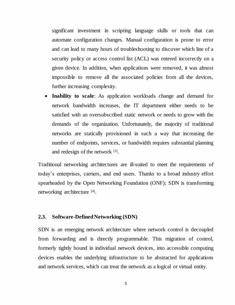
significant investment in scripting language skills or tools that can
automate configuration changes. Manual configuration is prone to error
and can lead to many hours of troubleshooting to discover which line of a
security policy or access control list (ACL) was entered incorrectly on a
given device. In addition, when applications were removed, it was almost
impossible to remove all the associated policies from all the devices,
further increasing complexity.
Inability to scale: As application workloads change and demand for
network bandwidth increases, the IT department either needs to be
satisfied with an oversubscribed static network or needs to grow with the
demands of the organization. Unfortunately, the majority of traditional
networks are statically provisioned in such a way that increasing the
number of endpoints, services, or bandwidth requires substantial planning
and redesign of the network [3].
Traditional networking architectures are ill-suited to meet the requirements of
today’s enterprises, carriers, and end users. Thanks to a broad industry effort
spearheaded by the Open Networking Foundation (ONF); SDN is transforming
networking architecture [4].
2.3. Software-Defined Networking (SDN)
SDN is an emerging network architecture where network control is decoupled
from forwarding and is directly programmable. This migration of control,
formerly tightly bound in individual network devices, into accessible computing
devices enables the underlying infrastructure to be abstracted for applications
and network services, which can treat the network as a logical or virtual entity.

6
As a result, enterprises and carriers gain unprecedented programmability,
automation, and network control, enabling them to build highly scalable, flexible
networks that readily adapt to changing business needs [4].
SDN are controlled by software applications and SDN controllers rather than the
traditional network management consoles and commands that required a lot of
administrative overhead and could be tedious to manage on a large scale [3].
2.3.1. SDN Architecture
Network intelligence is (logically) centralized in software-based SDN
controllers, which maintain a global view of the network. As a result, the
network appears to the applications and policy engines as a single, logical
switch. With SDN, enterprises and carriers gain vendor-independent control over
the entire network from a single logical point, which greatly simplifies the
network design and operation. SDN also greatly simplifies the network devices
themselves, since they no longer need to understand and process thousands of
protocol standards but merely accept instructions from the SDN controllers [4].
The figure 2-1 below depicts a logical view of the SDN architecture.
Figure 2-1: SDN Architecture.

7
SDN architectures support a set of APIs that make it possible to implement
common network services, including routing, multicast, security, access control,
bandwidth management, traffic engineering, quality of service, processor and
storage optimization, energy usage, and all forms of policy management, custom
tailored to meet business objectives. For example, an SDN architecture makes it
easy to define and enforce consistent policies across both wired and wireless
connections on a campus [4].
2.3.2. SDN Advantages
OpenFlow is the first standard interface designed specifically for SDN,
providing high-performance, granular traffic control across multiple vendors’
network devices. OpenFlow-based SDN is currently being rolled out in a variety
of networking devices and software, delivering substantial benefits to both
enterprises and carriers, including:
• Centralized management and control of networking devices from multiple
vendors.
• Improved automation and management by using common APIs to abstract
the underlying networking details from the orchestration and provisioning
systems and applications.
• Rapid innovation through the ability to deliver new network capabilities
and services without the need to configure individual devices or wait for
vendor releases.
• Programmability by operators, enterprises, independent software vendors,
and users (not just equipment manufacturers) using common programming

8
environments, which gives all parties new opportunities to drive revenue
and differentiation.
• Increased network reliability and security as a result of centralized and
automated management of network devices, uniform policy enforcement,
and fewer configuration errors.
• More granular network control with the ability to apply comprehensive
and wide-ranging policies at the session, user, device, and application
levels.
• Better end-user experience as applications exploit centralized network
state information to seamlessly adapt network behavior to user needs [4].
2.3.3. SDN Applications
To give an idea of how huge SDN is, the list below mentioned some of the
applications which is related to.
Appliance Virtualization: Firewalls, Load balancers, Content
distribution, and Gateways.
Service Assurance: Content-specific traffic routing for optimal Quality
of Experience (QoE), Congestion control based on network conditions,
Dynamic policy-based traffic engineering.
Service Differentiation: Value-add service features, Bandwidth-on-
demand features, BYOD across multiple networks, Service
insertion/changing.
Service Velocity: Virtual edge, distributed app testing environments,
Application development workflows.
9
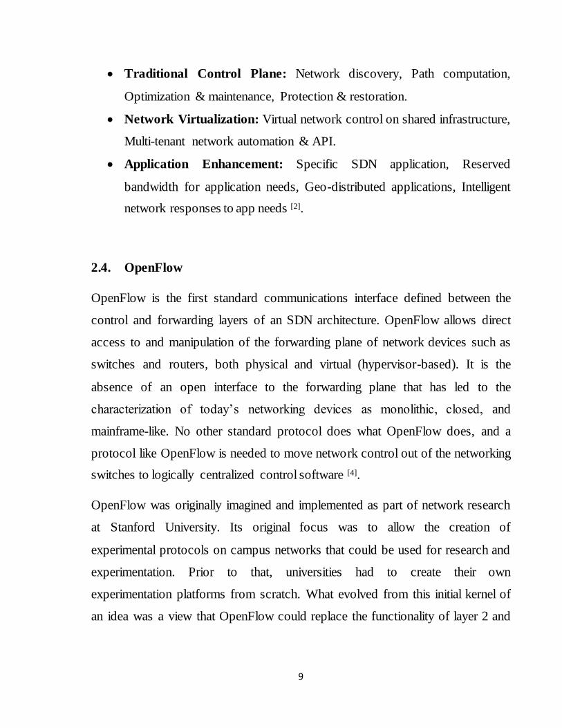
Traditional Control Plane: Network discovery, Path computation,
Optimization & maintenance, Protection & restoration.
Network Virtualization: Virtual network control on shared infrastructure,
Multi-tenant network automation & API.
Application Enhancement: Specific SDN application, Reserved
bandwidth for application needs, Geo-distributed applications, Intelligent
network responses to app needs [2].
2.4. OpenFlow
OpenFlow is the first standard communications interface defined between the
control and forwarding layers of an SDN architecture. OpenFlow allows direct
access to and manipulation of the forwarding plane of network devices such as
switches and routers, both physical and virtual (hypervisor-based). It is the
absence of an open interface to the forwarding plane that has led to the
characterization of today’s networking devices as monolithic, closed, and
mainframe-like. No other standard protocol does what OpenFlow does, and a
protocol like OpenFlow is needed to move network control out of the networking
switches to logically centralized control software [4].
OpenFlow was originally imagined and implemented as part of network research
at Stanford University. Its original focus was to allow the creation of
experimental protocols on campus networks that could be used for research and
experimentation. Prior to that, universities had to create their own
experimentation platforms from scratch. What evolved from this initial kernel of
an idea was a view that OpenFlow could replace the functionality of layer 2 and

10
layer 3 protocols completely in commercial switches and routers. This approach
is commonly referred to as the clean slate proposition [1].
In 2011, a nonprofit consortium called the Open Networking Foundation (ONF)
was formed by a group of service providers to commercialize, standardize, and
promote the use of OpenFlow in production networks [1].
2.4.1. OpenFlow applications
There is a wide range of applications, where use of OpenFlow can improve
overall system performance. The following list brings some of the experiments
(performed at the Stanford University) [8].
Slicing the network: The network infrastructure can be divided into
logical slices (using e.g. FlowVisor software). Hence, different services
can be mapped to different network slices, and the traffic could then be
treated accordingly.
Load balancing: The whole network can be viewed as one big software
load balancing switch instead of deploying expensive load balancing
hardware switches.
Packet and circuit network convergence: OpenFlow provides a solution
for merging packet and circuit networks into one, thus reducing
CAPEX/OPEX spending of telecommunications companies.
Reduction of energy consumption: The unused links can be switched
off, so that less energy is needed to run e.g. a data center network.
Dynamic flow aggregation: OpenFlow can help saving the resources
(CPU, routing tables) or further ease management of the network.

11
Providing MPLS services: OpenFlow can simplify deployment of new
MPLS services (e.g. new tunnels including adjustments of their bandwidth
reservation).
2.5. Network Load Balancing
Load balancing is very important in building high speed networks and also to
ensure high performance in the network backbone.
The main idea of load balancing is to map the part of the traffic from the heavily
loaded paths to some lightly loaded paths to avoid congestion in the shortest path
route and to increase the network utilization and network throughput.
Approached used for Load Balancing can be broadly classified in to following
types [9]:
2.5.1. Round Robin forwarding.
Per packet round robin scheduling is advantageous only when all the paths are of
equal cost. Otherwise packet disordering will take place which can be interpreted
as false congestion signals. This would lead in unnecessary degradation in the
throughput of the network leaving some links unutilized whereas at the same
time leading to the overutilization of the other links.
2.5.2. Time dependent approach:
Balancing traffic on the basis of long time span as per the experience of the
traffic.
Time dependent approach will vary the traffic on the basis of variations in the
traffic over a long time span. These types of approaches are insensitive to the
dynamic traffic variations.
12
2.5.3. Hashing based approaches.
Hashing based approaches are a stateless approach which applies the hash
function on subset of five tuples (source address, destination address, source
port, destination port and protocol id). This type of traffic splitting is fairly easy
to compute. Though, it maintains the flow based traffic splitting yet by this
method the traffic can- not be distributed unevenly. And more over as it does not
maintain the state so dynamic traffic engineering is not applicable to these types
of approaches.
2.5.4. Routing traffic as per the metrics calculated from the traffic.
Various authors have proposed traffic engineering with some calculated metrics
like packet delay or/and packet loss etc. dynamically and applying them to split
the traffic. This method is highly advantageous if the flow integrity is maintained
and if the metrics calculation overhead is not considerable.
2.6. Interconnection networks
Interconnection networks were traditionally defined as networks that connect
multiprocessors. However, interconnection networks evolved dramatically in the
last 20 years and nowadays play a crucial role in areas like Data Centers or high
performance computing (HPC) clusters.
Topologies for interconnection networks can be classified into four major
groups: shared-bus networks, direct networks, indirect networks and hybrid
networks. The choice of topology is one of the most important steps when
constructing an interconnection network. The chosen topology combined with
the routing algorithm and application’s workload determines the traffic
distribution in the network [10].
13
2.6.1. Fat-Tree topology
The fat-tree topology is very popular for building medium and large system area
networks [11]. It was invented by Charles E. Leiserson of the Massachusetts
Institute of Technology in 1985 [12].
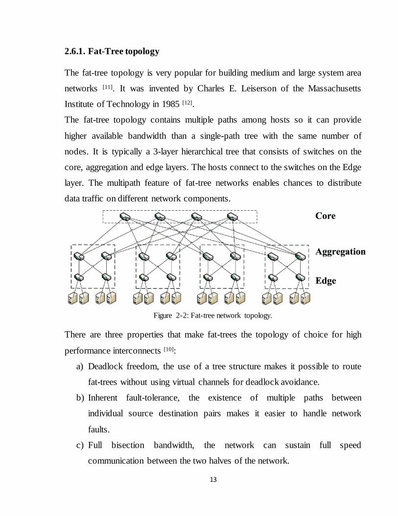
The fat-tree topology contains multiple paths among hosts so it can provide
higher available bandwidth than a single-path tree with the same number of
nodes. It is typically a 3-layer hierarchical tree that consists of switches on the
core, aggregation and edge layers. The hosts connect to the switches on the Edge
layer. The multipath feature of fat-tree networks enables chances to distribute
data traffic on different network components.
Figure 2-2: Fat-tree network topology.
There are three properties that make fat-trees the topology of choice for high
performance interconnects [10]:
a) Deadlock freedom, the use of a tree structure makes it possible to route
fat-trees without using virtual channels for deadlock avoidance.
b) Inherent fault-tolerance, the existence of multiple paths between
individual source destination pairs makes it easier to handle network
faults.
c) Full bisection bandwidth, the network can sustain full speed
communication between the two halves of the network.

14
Although the fat-tree topology provides rich connectivity, having a fat-tree
topology alone does not guarantee high network performance: the routing
mechanism also plays a crucial role. Historically, adaptive routing, which
dynamically builds the path for a packet based on the network condition, has
been used with the fat-tree topology to achieve load balance in the network.
However, the routing in the current major system area networking technology is
deterministic. For a fat-tree based system area network with deterministic
routing, it is important to employ an efficient load balance routing scheme in
order to fully exploit the rich connectivity provided by the fat-tree topology [11].
2.7. Dijkstra's algorithm
Dijkstra's algorithm, conceived by Dutch computer scientist Edsger Dijkstra in
1956 and published in 1959 [13][14], is a graph search algorithm that solves the
single-source shortest path problem for a graph with nonnegative edge path
costs, producing a shortest path tree.
This algorithm is often used in routing and as a subroutine in other graph
algorithms. For a given source vertex (node) in the graph, the algorithm finds the
path with lowest cost (i.e. the shortest path) between that vertex and every other
vertex.
It can also be used for finding costs of shortest paths from a single vertex to a
single destination vertex by stopping the algorithm once the shortest path to the
destination vertex has been determined. For example, if the vertices of the graph
represent cities and edge path costs represent driving distances between pairs of
cities connected by a direct road, Dijkstra's algorithm can be used to find the
shortest route between one city and all other cities. As a result, the shortest path

15
first is widely used in network routing protocols, most notably IS-IS and
OSPF[15].
2.8. SDN Dynamic Load Balancing Algorithm
This research algorithm takes into account the advantages and features of SDN,
which can sense the state of each of the elements on the network in order to act
consequently.
In order to describe the algorithm, first it is needed to disclose the different data
structures involved on it. Such structures characterize the different elements that
have been taken in account in order to achieve an efficient load balancing, at the
same time that to reduce as much as possible the computational cost and time [2].
The main data structures are explained bellow.
a) Flow
Since the algorithm provides load balancing based on flows, it is necessary to
define a structure to describe each of the different flows with distinctive
parameters.
Notice that for the goal of this research have been taking in account the IP
sand Ports, but using OpenFlow it is possible to make a much more accurate
identification of each flow with any of the header fields.
A Flow structure specifies a specific traffic flow from one host to another one.
The structure is as follows:
Flow = {<FlowID>, <SrcIP>, <DstIP>, <SrcPort>, <DstPort>,<UsedBandwidth>}
FlowID: identify each flow with a unique ID.

16
SrcIP: this field contains the IPv4 of the source host who initialized a flow.
DstIP: IPv4 of the destination host.
SrcPort: port number of the source.
DstPort: port number of the destination.
UsedBandwidth: transmission speed of a specific flow, in Mbps.
b) Flows Collection
Groups of flows are put together in collections, which contain a number of
flows with common characteristic (e.g. flows that goes through a same link).
FlowsCollection={< Flow 1 >,< Flow2 > ... < Flow n >}
c) Path
Keeping information about each parallel route between each pair of hosts it is
crucial to be able to redirect the flows according to the current network
conditions. To accomplish that tracking, a data structure representing each of
the possible paths has been designed.
A Path structure contains the information about a precise path between two
hosts, and it is composed as shown below:
Path={<PathID>,<Hops>,<Links>,<Ingress>,<Egress>,<Capacity>,< Flows>,
<UsedBandwidth>, <FreeCapacity>}
PathID: identify each single possible path with a unique ID.
Hops: contains a identifier of each of the switches within the path.
Links: list of all the links involved in the path. Each of the links is composed
by a pair of Switch-Port identifiers.

17
Ingress: identifier of the switch with the source host is connected to.
Egress: identifier of the switch with the destination host is connected to.
Capacity: specify the maximum capacity of the path. Which corresponds to
the capacity of the link with smallest capacity along the path.
Flows: list of flows which are routed through this path.
Used Bandwidth: sum of the traffic of all the flows that are using this path, in
Mbps.
Free Capacity: capacity available in this path. It’s the minimum capacity free
of the Links that shape the path.
d) Paths Collection
Path Collection contains a list of all the possible paths of the hosts that have
initiated a communication between them, and information about each of the
paths [2].
PathsCollection={< Path 1 >,< Path2 > ... < Path n >}
2.9. Literature Review
In 2014, Yuanhao Zhou, Li Ruan, Limin Xiao andRui Liu published the paper
“A Method for Load Balancing based on Software-Defined Network”. The paper
presented a method for load balancing based on SDN. It implemented load
balancing according to PyResonance controller. PyResonance is Resonance
implemented with Pyretic. Resonance is an SDN control platform that advocates
event-driven network control. It preserves a Finite State Machine (FSM) model

18
to define a network policy. The paper showed that traffic can be distributed more
efficiently and easily with the aid of the proposed solution [5].
In May 2015, Senthil Ganesh N and Ranjani S. published the paper “Dynamic
Load Balancing using Software Defined Networks”. In this paper a Software-
Defined Network using OpenFlow protocol was implemented to improve the
efficiency of load balancing in enterprise networks. By using this technique, the
network becomes directly programmable and agile. Here the http requests from
different clients will be directed to different pre-defined http servers based on
Round-Robin scheduling. Round-Robin scheduling is easy to implement and are
good to be used in geographically distributed web servers [6].
In June 2015, Smriti Bhandarkar and Kotla Amjath Khan published the paper
“Load Balancing in Software-defined Network (SDN) Based on Traffic
Volume”. The paper showed that the key limitations are statically configured
forwarding plane and uneven load balancing among the controllers in the
network. It proposed The dynamic load balancer which dynamically shifts the
load to the other shortest path when it is greater than the bandwidth of the link.
By experimental analysis, the paper concluded that the proposed approach gives
better results in terms of responses/sec and efficiency as compared with the
existing Round-Robin load balancing algorithm [7].

Chapter Three
Methodology

19
Chapter Three
Methodology
3.1. Introduction
This chapter describes the algorithm designed to accomplish a dynamic load
balancing system, and presents the components and software tools used in this
research to set the testbed.
3.2. Algorithm Description
As explained formerly, the task of the Nayan Seth’s algorithm[19] is to distribute
traffic of upcoming and incoming network flows in order to achieve the best
possible resource utilization of each of the links present in a network. In order to
achieve such aim, it is necessary to keep track of the current state of the network.
Figure 3-1 illustrates the steps of the load balancing algorithm.

20
Figure 3-1: SDN Dynamic Load Balancing algorithm.
The first step of the algorithm is to collect operational information of the
topology and its devices. Such as IPs, MAC addresses, Ports, Connections, etc.

21
Next step is to find route information based on Dijkstra's algorithm (see Chapter
2 section 8), the goal here is to narrow the search into a small segment of the Fat-
Tree topology and to find the shortest paths from source host to destination host.
And then find total link cost for all these paths between the source and
destination hosts.
Once the transmission costs of the links are calculated, the flows are created
depending on the minimum transmission cost of the links at the given time.
Based on the cost, the best path is selected and static flows are pushed into each
switch in the current best path. with that, every switch within the selected path
will have the necessary flow entries to carry out the communication between the
two end points.
Finally, the program continues to update this information every minute thereby
making it dynamic.
3.3. Implementation Overview
In this research a test-bed has been implemented under Linux, using Mininet
software to emulate the network, the open-source OpenDaylight platform (ODL)
as SDN controller, and Python programming language to define the fat-tree
topology and to write the load balancing algorithm program, and iPerf to test
network performance. The following diagram illustrate the design steps.

22
3.4. Components and Software Tools
3.4.1. Mininet
Mininet is a network emulator that allows prototyping large networks on a single
machine. It runs a collection of end-hosts, switches, routers, and links on a single
Linux kernel. It uses lightweight virtualization to make a single system look like
a complete network, running the same kernel, system, and user code.
Mininet main advantages:
1. Mininet is an open source project.
2. Custom topologies can be created.
3. Mininet runs real programs.
4. Packet forwarding can be customized.
Setting a Linux Environment -
Ubuntu 14.04 LTS
Install Java SE Development Kit
(JDK)
Download and install Mininet
Download the OpenDaylight
Platform
Install OpenDaylight
features
Install Python libraries and
modules
Define Fat-tree network
topology using Python
Run OpenDaylight
Controller
Run the network topology in Mininet,
and set it to use OpenDaylight as its
controller
Test network performance using iPerf
Run the Dynamic Load balancing
algorithm program
Test network performance
using iPerf after LB
Results and Performance
analysis

23
Compared to simulators, Mininet runs real, unmodified code including
application code, OS kernel code, and control plane code (both OpenFlow
controller code and Open vSwitch code) and easily connects to real networks.
3.4.2. The OpenDaylight Project (ODL)
The OpenDaylight Project (ODL) is a highly available, modular, extensible,
scalable and multi-protocol controller infrastructure built for SDN deployments
on modern heterogeneous multi-vendor networks. ODL provides a model-driven
service abstraction platform that allows users to write apps that easily work
across a wide variety of hardware and south-bound protocols.
Furthermore, it contains internal plugins that add services and functionalities to
the network. For example, it has dynamic plugins that allow to gather statistics
as well as to obtain the topology of the network [17].
Figure 3-2: Beryllium-SR4 architecture framework.

24
3.4.3. iPerf
iPerf is a commonly used network testing tool for measuring Transmission
Control Protocol (TCP) and User Datagram Protocol (UDP) bandwidth
performance and the quality of a network link. By tuning of various parameters
related to timing, buffers and protocols (TCP, UDP, SCTP with IPv4 and IPv6),
the user is able to perform a number of tests that provide an insight on the
network's bandwidth availability, delay, jitter and data loss.iPerf is an open
source software and runs on various platforms including Linux, UNIX and
Windows.
Figure 3-3: iPerf Bandwidth measurement.
3.4.4. Programming Language used: Python
In this research, Python has been used in mininet to define the Fat-tree topology,
also it has been used to write the load balancing algorithm program.
Python is an interpreted, object-oriented language suitable for many purposes. It
has a clear, intuitive syntax, powerful high-level data structures, and a flexible
dynamic type system. Python can be used interactively, in stand-alone scripts,
for large programs, or as an extension language for existing applications. The
language runs on Linux, Macintosh, and Windows machines [18].

25
Python is easily extensible through modules written in C or C++, and can also be
embedded in applications as a library. There are also a number of system-specific
extensions. A large library of standard modules written in Python also exists.
Compared to C, Python programs are much shorter, and consequently much
faster to write. In comparison with Perl, Python code is easier to read, write and
maintain. Relative to TCL, Python is better suited for larger or more complicated
programs [18].

Chapter Four
Results and Performance Evaluation

26
Chapter Four
Results and Performance Evaluation
4.1. Introduction
This chapter describes the proposed scenarios, then shows and explains the results
obtained with the scenarios proposed.
4.2. Network Topology
The network topology used in this research is a three-levels fat-tree Data Center
topology. It consists of 8 servers, 4 edge switches, 4 aggregation switches, and 2
core switches. As presented in Figure 4-1.
Figure 4-1: Datacenter Network Topology used.

27
4.3. Scenario Description
4.3.1. First Scenario: Performance Measurement at the Aggregation Layer
In this scenario the severs h1 and h4 has been selected to perform the load
balancing between them. As shown is the figure 4-2 below.
Figure 4-2: The selected hosts and possible paths in the first scenario.
The network was tested before and after running the load balancing algorithm. The
testing focused on some of QoS parameters such as throughput, delay, jitter, and
packet loss between the two servers in the fat-tree network.
Delay has been measured by sending five Internet Control Message Protocol
(ICMP) Echo Request packets to the destination host and calculated the time until
ICMP Echo Reply was received at the source host.
Throughput, Jitter, and Packet Loss has been tested using iPerf, first case by using
the TCP and then by using UDP, with 10 seconds for each test.
The following figures 4-3 to 4-5 show examples of the testing results.

28
Figure 4-3: ping from h1 to h4 before load balancing.
Figure 4-4: iPerf h1 to h4 before load balancing – TCP connection.

29
Figure 4-5: iPerf h1 to h4 before load balancing – UDP connection.
4.3.1.1. Tests results of the first scenario
The network was tested ten times before and after running the load balancing
algorithm; to study any abnormal behavior. The following table illustrates the
results obtained.
Table 4-1: Tests results of the first scenario.
Test
No.
Load
Balancing
TCP UDP Delay
(ms) Throughput
(Mbits/sec)
Transfer
(Mbytes)
Throughput
(Mbits/sec)
Transfer
(Mbytes)
Jitter
(ms)
Packet
Loss %
1 Before 191 228 354 422 0.641 15% 0.297
After 13414.4 15564.8 524 594 0.081 13% 0.142
2 Before 221 265 299 357 0.325 38% 0.496
After 28262.4 32870.4 726 866 0.011 5% 0.176
3 Before 255 304 274 327 0.521 59% 0.203
After 16076.8 18739.2 713 849 0.006 6% 0.09
4 Before 185 220 361 431 0.491 52% 0.578

30
After 21196.8 24678.4 765 912 0.001 2% 0.101
5 Before 238 284 228 278 14.67 35% 0.69
After 28876.8 33689.6 653 778 0.005 11% 0.159
6 Before 184 223 283 338 0.42 41% 0.529
After 26828.8 31334.4 625 745 0.176 12% 0.16
7 Before 208 249 256 305 0.365 30% 0.518
After 30617.6 35635.2 743 885 0.014 4% 0.133
8 Before 233 278 298 355 0.543 36% 0.425
After 34201.6 39833.6 738 880 0.013 5% 0.115
9 Before 236 281 255 304 0.691 43% 0.707
After 24268.8 28262.4 742 885 0.193 4% 0.152
10 Before 244 292 215 256 0.172 42% 0.708
After 36761.6 42803.2 740 881 0.015 3% 0.144
To summarize the previous table, an average performance has been calculated as
shown in the following table.
Table 4-2: Average results of the first scenario.
Load
Balancing
TCP UDP Delay
(ms) Throughput
(Mbits/sec)
Transfer
(Mbytes)
Throughput
(Mbits/sec)
Transfer
(Mbytes)
Jitter
(ms)
Packet
Loss %
Before 219.5 262.4 282.3 337.3 1.884 39.10% 0.5151
After 26050.56 30341.12 696.9 827.5 0.0515 6.43% 0.1372
4.3.1.2. Performance Analysis of the first scenario
The network showed a much better performance in the first scenario after running
the load balancing program. The average network Throughput before load
balancing was 219.5 Mbits/sec, and it became 25.4 Gbits/sec after load balancing.
The average delay has decreased by 73.36% after load balancing with an average
of 0.1372 ms, the Jitter has decreased by 97.27%, and the Packet Loss has
decreased by 32.67%.

31
Figure 4-6: Comparison of Throughput tests results in first scenario.
Figure 4-7: Comparison of QoS parameters in first scenario.
219.5 262.4 282.3 337.3
26050.56
30341.12
696.9 827.5
0
5000
10000
15000
20000
25000
30000
35000
TCP - Throughput(Mbits/sec)
TCP - Transfer(Mbytes)
UDP - Throughput(Mbits/sec)
UDP - Transfer(Mbytes)
Before After
1.884
39.10%0.5151
0.0515 6.43%0.1372
0
0.2
0.4
0.6
0.8
1
1.2
1.4
1.6
1.8
2
Jitter (ms) Packet Loss % Delay (ms)
Before After

32
4.3.2. Second Scenario: Performance Measurement at the Core Layer
In this scenario the severs h1 and h6 has been selected to perform the load
balancing between them. In this scenario the traffic will have to go through the
core switches in order to reach its destination. The figure 4-8 below shows the
selected hosts and the possible paths.
Figure 4-8: The selected hosts and possible paths in the second scenario.
The network was tested before and after running the load balancing algorithm. The
testing focused on some of QoS parameters such as throughput, delay, jitter, and
packet loss between the two servers in the fat-tree network.
The following figures 4-9 to 4-11 show examples of the testing results.

33
Figure 4-9: ping from h1 to h6 before load balancing.
Figure 4-10: iPerf h1 to h6 before load balancing – TCP connection.

34
Figure 4-11: iPerf h1 to h6 before load balancing – UDP connection.
4.3.2.1. Tests results of the second scenario
The network was tested ten times before and after running the load balancing
algorithm; to study any abnormal behavior. The following table illustrates the
results obtained.
Table 4-3: Tests results of the second scenario.
Test
No.
Load
Balancing
TCP UDP Delay
(ms) Throughput
(Mbits/sec)
Transfer
(Mbytes)
Throughput
(Mbits/sec)
Transfer
(Mbytes)
Jitter
(ms)
Packet
Loss %
1 Before 195 234 291 347 0.121 34% 0.552
After 268 319 263 313 0.438 51% 0.439
2 Before 194 233 225 268 0.061 54% 0.268
After 273 326 336 401 0.529 52% 0.323
3 Before 150 179 147 176 0.889 39% 0.943
After 215 257 203 242 0.529 42% 0.561
4 Before 183 219 201 239 0.292 34% 0.374

35
After 240 287 238 288 14.12 44% 0.401
5 Before 187 225 194 231 0.564 45% 0.242
After 236 283 232 283 14.32 36% 0.662
6 Before 219 261 226 268 0.166 36% 0.553
After 288 344 380 453 0.567 51% 0.618
7 Before 203 243 246 293 0.691 46% 0.566
After 222 266 367 437 0.537 53% 0.499
8 Before 164 196 225 268 0.128 28% 0.596
After 220 263 252 299 0.587 35% 0.432
9 Before 220 264 258 307 0.415 38% 0.615
After 301 359 281 335 0.335 38% 0.332
10 Before 176 210 179 213 0.409 40% 0.582
After 239 288 234 280 0.913 41% 0.54
To summarize the previous table, an average performance has been calculated as
shown in the following table.
Table 4-4: Average results of the second scenario.
Load
Balancing
TCP UDP Delay
(ms) Throughput
(Mbits/sec)
Transfer
(Mbytes)
Throughput
(Mbits/sec)
Transfer
(Mbytes)
Jitter
(ms)
Packet
Loss %
Before 189.1 226.4 219.2 261 0.3736 39.40% 0.5291
After 250.2 299.2 278.6 333.1 3.2891 44.30% 0.4807
4.3.2.2. Performance Analysis of the second scenario
In the second scenario, the network showed good performance after running the
load balancing program. The average network throughput was 189.1 Mbits/sec,
and it became 250.2 Mbits/sec after load balancing with 32.3% increasing
percentage. The average delay has decreased by 9.15% after load balancing with
an average of 0.4807ms. But the average jitter has increased from 0.3736 ms to
3.2891 ms after the load balancing, and the packet loss has also increased by 4.9%.

36
The load balancing program managed to increase the throughput in all cases. It
showed a great performance under the second layer of the fat-tree topology, but as
the network grows larger and the core layer gets involved, it presents increasing
in the packet loss and jitter.
Figure 4-12: Comparison of Throughput tests results in second scenario.
Figure 4-13: Comparison of QoS parameters in second scenario.
189.1
226.4 219.2
261250.2
299.2278.6
333.1
0
50
100
150
200
250
300
350
TCP - Throughput(Mbits/sec)
TCP - Transfer(Mbytes)
UDP - Throughput(Mbits/sec)
UDP - Transfer(Mbytes)
Before After
0.3736 39.4%0.5291
3.2891
44.3% 0.4807
0
0.5
1
1.5
2
2.5
3
3.5
Jitter (ms) Packet Loss % Delay (ms)
Before After

Chapter Five
Conclusion and Recommendations for Future Work

37
Chapter Five
Conclusion and Recommendations for Future Work
5.1. Conclusion
This research describes the implementation of Nayan Seth’s dynamic load
balancing algorithm to efficiently distribute flows for fat-tree networks through
multiple alternative paths between a single pair of hosts.
The network was tested before and after running the load balancing algorithm. The
testing focused on some of QoS parameters such as throughput, delay, and packet
loss between two servers in the fat-tree network.
The results showed that the network performance has increased after running the
load balancing algorithm program, the algorithm was able to increase throughput,
and improve network utilization. However, in large networks it increased packet
loss and jitter.
5.2. Recommendations for Future Work
In future work, next suggestions are planned: The first suggestion is to investigate
the performances of the dynamic load balancing program on a different popular
SDN controllers, such as Research Floodlight, Beacon, NOX/POX, etc. and
compare the results.
The second suggestion is to investigate the performances of different topologies
of different sizes, other than the fat-tree topology. To test if there are any other
limitations with the algorithm.
And finally is to extend the algorithm to traditional networks, or hybrid networks
with both OpenFlow and regular switches.

38
References
[1] Thomas D. Nadeau and Ken Gray. “SDN: Software Defined Networks”.
O'Reilly Media, Inc. Ebook, 1st edition, 9-20. August 2013.
[2] Martí Boada Navarro. “Dynamic Load Balancing in Software-Defined
Networks”. Aalborg University, Department of Electronic Systems, Fredrik
Bajers Vej 7B, DK-9220 Aalborg. June 2014.
[3] Brian Underdahl and Gary Kinghorn. “Software Defined Networking for
Dummies”, Cisco Special Edition, John Wiley & Sons, Inc., Hoboken, New
Jersey, 2015.
[4] “Software-Defined Networking: The New Norm for Networks”. Open
Networking Foundation (ONF), White Paper. April 13, 2012.
[5] Yuanhao Zhou, Li Ruan, Limin Xiao and Rui Liu. “A Method for Load
Balancing based on Software-Defined Network”. Advanced Science and
Technology Letters, Vol.45 (CCA 2014), pp.43-48, 2014.
[6] Senthil Ganesh N and Ranjani S. “Dynamic Load Balancing using Software
Defined Networks”. International Journal of Computer Applications (0975 –
8887), International Conference on Current Trends in Advanced Computing
(ICCTAC-2015), May 2015.
[7] Smriti Bhandarkar and Kotla Amjath Khan. “Load Balancing in Software-
defined Network (SDN) Based on Traffic Volume”. Advances in Computer
Science and Information Technology (ACSIT), Krishi Sanskriti Publications,
Volume 2, Number 7; April – June, 2015.
[8] Petr Marciniak. “Load Balancing in OpenFlow Networks”. Department of
Information Systems, Faculty of Information Technology, Brno University
of Technology. Brno, Czech Republic, 2013.

39
[9] Ravindra Kumar Singh, Narendra S. Chaudhari, and Kanak Saxena. “Load
Balancing in IP/MPLS Networks: A Survey”. Published online by Scientific
Research Corporation (SciRes). Atlanta, March 15, 2012.
[10] Bartosz Bogda´nski. “Optimized Routing for Fat-Tree Topologies”.
Department of Informatics, Faculty of Mathematics and Natural Sciences,
University of Oslo, Norway. January, 2014.
[11] Xin Yuan, Wickus Nienaber, Zhenhai Duan, Rami Melhem. “Oblivious
Routing for Fat-Tree Based System Area Networks with Uncertain Traffic
Demands”. SIGMETRICS’07, June 12-16, San Diego, California, USA. 2007.
[12] Charles E. Leiserson. “Fat-trees: universal networks for hardware-efficient
supercomputing”. IEEE Transactions on Computers, Vol. 34 , no. 10, Oct. 1985,
pp. 892-901.
[13] Dijkstra, E. W. (1959). "A note on two problems in connexion with graphs"
(http:/ / www-m3. ma. tum. de/ twiki/ pub/ MN0506/ WebHome/ dijkstra. pdf).
Numerische Mathematik 1: 269–271. doi:10.1007/BF01386390.
[14] Cormen, Thomas H.; Leiserson, Charles E.; Rivest, Ronald L.; Stein, Clifford
(2001). "Section 24.3: Dijkstra's algorithm". Introduction to Algorithms (Second
ed.). MIT Press and McGraw-Hill. pp. 595–601. ISBN 0-262-03293-7.
[15] Fredman, Michael Lawrence; Tarjan, Robert E. (1984). "Fibonacci heaps and
their uses in improved network optimization algorithms". 25th Annual
Symposium on Foundations of Computer Science (IEEE): 338–346.
doi:10.1109/SFCS.1984.715934.
[16] Fredman, Michael Lawrence; Tarjan, Robert E. (1987). "Fibonacci heaps and
their uses in improved network optimization algorithms" (http:/ / portal. acm. org/
citation. cfm?id=28874). Journal of the Association for Computing Machinery 34
(3): 596–615. doi:10.1145/28869.28874.

40
[17] Bernat Ribes Garcia. “OpenDaylight SDN controller platform”. Faculty of
the Escola Tècnica d'Enginyeria de Telecomunicació de Barcelona, Universitat
Politècnica de Catalunya. Barcelona, October 2015.
[18] Guido van Rossum. “An Introduction to Python for UNIX/C Programmers”.
Proceedings of the NLUUG najaarsconferentie. Amsterdam, Netherlands, 1993.
[19] Nayan Seth. April, 2016. SDN Load Balancing. Retrieved from
https://github.com/nayanseth/sdn-loadbalancing
41
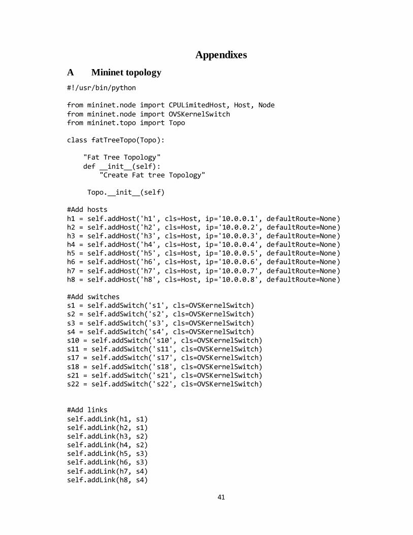
Appendixes
A Mininet topology
#!/usr/bin/python from mininet.node import CPULimitedHost, Host, Node from mininet.node import OVSKernelSwitch from mininet.topo import Topo class fatTreeTopo(Topo): "Fat Tree Topology" def __init__(self): "Create Fat tree Topology" Topo.__init__(self) #Add hosts h1 = self.addHost('h1', cls=Host, ip='10.0.0.1', defaultRoute=None) h2 = self.addHost('h2', cls=Host, ip='10.0.0.2', defaultRoute=None) h3 = self.addHost('h3', cls=Host, ip='10.0.0.3', defaultRoute=None) h4 = self.addHost('h4', cls=Host, ip='10.0.0.4', defaultRoute=None) h5 = self.addHost('h5', cls=Host, ip='10.0.0.5', defaultRoute=None) h6 = self.addHost('h6', cls=Host, ip='10.0.0.6', defaultRoute=None) h7 = self.addHost('h7', cls=Host, ip='10.0.0.7', defaultRoute=None) h8 = self.addHost('h8', cls=Host, ip='10.0.0.8', defaultRoute=None) #Add switches s1 = self.addSwitch('s1', cls=OVSKernelSwitch) s2 = self.addSwitch('s2', cls=OVSKernelSwitch) s3 = self.addSwitch('s3', cls=OVSKernelSwitch) s4 = self.addSwitch('s4', cls=OVSKernelSwitch) s10 = self.addSwitch('s10', cls=OVSKernelSwitch) s11 = self.addSwitch('s11', cls=OVSKernelSwitch) s17 = self.addSwitch('s17', cls=OVSKernelSwitch) s18 = self.addSwitch('s18', cls=OVSKernelSwitch) s21 = self.addSwitch('s21', cls=OVSKernelSwitch) s22 = self.addSwitch('s22', cls=OVSKernelSwitch) #Add links self.addLink(h1, s1) self.addLink(h2, s1) self.addLink(h3, s2) self.addLink(h4, s2) self.addLink(h5, s3) self.addLink(h6, s3) self.addLink(h7, s4) self.addLink(h8, s4)

42
self.addLink(s1, s21) self.addLink(s21, s2) self.addLink(s1, s10) self.addLink(s2, s10) self.addLink(s3, s11) self.addLink(s4, s22) self.addLink(s11, s4) self.addLink(s3, s22) self.addLink(s21, s17) self.addLink(s11, s17) self.addLink(s10, s18) self.addLink(s22, s18) topos = { 'mytopo': (lambda: fatTreeTopo() ) }

43
B Load balancing algorithm program
#!/usr/bin/env python # Orignal Code written by: Nayan Seth # Date: Apr 26, 2016 import requests from requests.auth import HTTPBasicAuth import json import unicodedata from subprocess import Popen, PIPE import time import networkx as nx from sys import exit # Method To Get REST Data In JSON Format def getResponse(url,choice): response = requests.get(url, auth=HTTPBasicAuth('admin', 'admin')) if(response.ok): jData = json.loads(response.content) if(choice=="topology"): topologyInformation(jData) elif(choice=="statistics"): getStats(jData) else: response.raise_for_status() def topologyInformation(data): global switch global deviceMAC global deviceIP global hostPorts global linkPorts global G global cost for i in data["network-topology"]["topology"]: for j in i["node"]: # Device MAC and IP if "host-tracker-service:addresses" in j: for k in j["host-tracker-service:addresses"]: ip = k["ip"].encode('ascii','ignore') mac = k["mac"].encode('ascii','ignore') deviceMAC[ip] = mac deviceIP[mac] = ip # Device Switch Connection and Port if "host-tracker-service:attachment-points" in j:

44
for k in j["host-tracker-service:attachment-points"]: mac = k["corresponding-tp"].encode('ascii','ignore') mac = mac.split(":",1)[1] ip = deviceIP[mac] temp = k["tp-id"].encode('ascii','ignore') switchID = temp.split(":") port = switchID[2] hostPorts[ip] = port switchID = switchID[0] + ":" + switchID[1] switch[ip] = switchID # Link Port Mapping for i in data["network-topology"]["topology"]: for j in i["link"]: if "host" not in j['link-id']: src = j["link-id"].encode('ascii','ignore').split(":") srcPort = src[2] dst = j["destination"]["dest-tp"].encode('ascii','ignore').split(":") dstPort = dst[2] srcToDst = src[1] + "::" + dst[1] linkPorts[srcToDst] = srcPort + "::" + dstPort G.add_edge((int)(src[1]),(int)(dst[1])) def getStats(data): print "\nCost Computation....\n" global cost txRate = 0 for i in data["node-connector"]: tx = int(i["opendaylight-port-statistics:flow-capable-node-connector-statistics"]["packets"]["transmitted"]) rx = int(i["opendaylight-port-statistics:flow-capable-node-connector-statistics"]["packets"]["received"]) txRate = tx + rx #print txRate time.sleep(2) response = requests.get(stats, auth=HTTPBasicAuth('admin', 'admin')) tempJSON = "" if(response.ok): tempJSON = json.loads(response.content) for i in tempJSON["node-connector"]: tx = int(i["opendaylight-port-statistics:flow-capable-node-connector-statistics"]["packets"]["transmitted"])
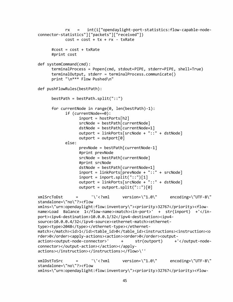
45
rx = int(i["opendaylight-port-statistics:flow-capable-node-connector-statistics"]["packets"]["received"]) cost = cost + tx + rx - txRate #cost = cost + txRate #print cost def systemCommand(cmd): terminalProcess = Popen(cmd, stdout=PIPE, stderr=PIPE, shell=True) terminalOutput, stderr = terminalProcess.communicate() print "\n*** Flow Pushed\n" def pushFlowRules(bestPath): bestPath = bestPath.split("::") for currentNode in range(0, len(bestPath)-1): if (currentNode==0): inport = hostPorts[h2] srcNode = bestPath[currentNode] dstNode = bestPath[currentNode+1] outport = linkPorts[srcNode + "::" + dstNode] outport = outport[0] else: prevNode = bestPath[currentNode-1] #print prevNode srcNode = bestPath[currentNode] #print srcNode dstNode = bestPath[currentNode+1] inport = linkPorts[prevNode + "::" + srcNode] inport = inport.split("::")[1] outport = linkPorts[srcNode + "::" + dstNode] outport = outport.split("::")[0] xmlSrcToDst = '\'<?xml version=\"1.0\" encoding=\"UTF-8\" standalone=\"no\"?><flow xmlns=\"urn:opendaylight:flow:inventory\"><priority>32767</priority><flow-name>Load Balance 1</flow-name><match><in-port>' + str(inport) +'</in-port><ipv4-destination>10.0.0.1/32</ipv4-destination><ipv4-source>10.0.0.4/32</ipv4-source><ethernet-match><ethernet-type><type>2048</type></ethernet-type></ethernet-match></match><id>1</id><table_id>0</table_id><instructions><instruction><order>0</order><apply-actions><action><order>0</order><output-action><output-node-connector>' + str(outport) +'</output-node-connector></output-action></action></apply-actions></instruction></instructions></flow>\'' xmlDstToSrc = '\'<?xml version=\"1.0\" encoding=\"UTF-8\" standalone=\"no\"?><flow xmlns=\"urn:opendaylight:flow:inventory\"><priority>32767</priority><flow-
46
name>Load Balance 2</flow-name><match><in-port>' + str(outport) +'</in-port><ipv4-destination>10.0.0.4/32</ipv4-destination><ipv4-source>10.0.0.1/32</ipv4-source><ethernet-match><ethernet-type><type>2048</type></ethernet-type></ethernet-match></match><id>2</id><table_id>0</table_id><instructions><instruction><order>0</order><apply-actions><action><order>0</order><output-action><output-node-connector>' + str(inport) +'</output-node-connector></output-action></action></apply-actions></instruction></instructions></flow>\'' flowURL = "http://127.0.0.1:8181/restconf/config/opendaylight-inventory:nodes/node/openflow:"+ bestPath[currentNode] +"/table/0/flow/1" command = 'curl --user "admin":"admin" -H "Accept: application/xml" -H "Content-type: application/xml" -X PUT ' + flowURL + ' -d ' + xmlSrcToDst systemCommand(command) flowURL = "http://127.0.0.1:8181/restconf/config/opendaylight-inventory:nodes/node/openflow:"+ bestPath[currentNode] +"/table/0/flow/2" command = 'curl --user "admin":"admin" -H "Accept: application/xml" -H "Content-type: application/xml" -X PUT ' + flowURL + ' -d ' + xmlDstToSrc systemCommand(command) srcNode = bestPath[-1] prevNode = bestPath[-2] inport = linkPorts[prevNode + "::" + srcNode] inport = inport.split("::")[1] outport = hostPorts[h1] xmlSrcToDst = '\'<?xml version=\"1.0\" encoding=\"UTF-8\" standalone=\"no\"?><flow xmlns=\"urn:opendaylight:flow:inventory\"><priority>32767</priority><flow-name>Load Balance 1</flow-name><match><in-port>' + str(inport) +'</in-port><ipv4-destination>10.0.0.1/32</ipv4-destination><ipv4-source>10.0.0.4/32</ipv4-source><ethernet-match><ethernet-type><type>2048</type></ethernet-type></ethernet-match></match><id>1</id><table_id>0</table_id><instructions><instruction><order>0</order><apply-actions><action><order>0</order><output-action><output-node-connector>' + str(outport) +'</output-node-connector></output-action></action></apply-actions></instruction></instructions></flow>\'' xmlDstToSrc = '\'<?xml version=\"1.0\" encoding=\"UTF-8\" standalone=\"no\"?><flow xmlns=\"urn:opendaylight:flow:inventory\"><priority>32767</priority><flow-name>Load Balance 2</flow-name><match><in-port>' + str(outport) +'</in-port><ipv4-destination>10.0.0.4/32</ipv4-destination><ipv4-

47
source>10.0.0.1/32</ipv4-source><ethernet-match><ethernet-type><type>2048</type></ethernet-type></ethernet-match></match><id>2</id><table_id>0</table_id><instructions><instruction><order>0</order><apply-actions><action><order>0</order><output-action><output-node-connector>' + str(inport) +'</output-node-connector></output-action></action></apply-actions></instruction></instructions></flow>\'' flowURL = "http://127.0.0.1:8181/restconf/config/opendaylight-inventory:nodes/node/openflow:"+ bestPath[-1] +"/table/0/flow/1" command = 'curl --user \"admin\":\"admin\" -H \"Accept: application/xml\" -H \"Content-type: application/xml\" -X PUT ' + flowURL + ' -d ' + xmlSrcToDst systemCommand(command) flowURL = "http://127.0.0.1:8181/restconf/config/opendaylight-inventory:nodes/node/openflow:"+ bestPath[-1] +"/table/0/flow/2" command = 'curl --user "admin":"admin" -H "Accept: application/xml" -H "Content-type: application/xml" -X PUT ' + flowURL + ' -d ' + xmlDstToSrc systemCommand(command) # Main # Stores H1 and H2 from user global h1,h2,h3 h1 = "" h2 = "" print "Enter Host 1" h1 = int(input()) print "\nEnter Host 2" h2 = int(input()) print "\nEnter Host 3 (H2's Neighbour)" h3 = int(input()) h1 = "10.0.0." + str(h1) h2 = "10.0.0." + str(h2) h3 = "10.0.0." + str(h3) flag = True while flag: #Creating Graph G = nx.Graph() # Stores Info About H3 And H4's Switch switch = {} # MAC of Hosts i.e. IP:MAC deviceMAC = {} # IP of Hosts i.e. MAC:IP deviceIP = {}
48
# Stores Switch Links To H3 and H4's Switch switchLinks = {} # Stores Host Switch Ports hostPorts = {} # Stores Switch To Switch Path path = {} # Stores Link Ports linkPorts = {} # Stores Final Link Rates finalLinkTX = {} # Store Port Key For Finding Link Rates portKey = "" # Statistics global stats stats = "" # Stores Link Cost global cost cost = 0 try: # Device Info (Switch To Which The Device Is Connected & The MAC Address Of Each Device) topology = "http://127.0.0.1:8181/restconf/operational/network-topology:network-topology" getResponse(topology,"topology") # Print Device:MAC Info print "\nDevice IP & MAC\n" print deviceMAC # Print Switch:Device Mapping print "\nSwitch:Device Mapping\n" print switch # Print Host:Port Mapping print "\nHost:Port Mapping To Switch\n" print hostPorts # Print Switch:Switch Port:Port Mapping print "\nSwitch:Switch Port:Port Mapping\n" print linkPorts # Paths print "\nAll Paths\n" #for path in nx.all_simple_paths(G, source=2, target=1): #print(path) for path in nx.all_shortest_paths(G, source=int(switch[h2].split(":",1)[1]), target=int(switch[h1].split(":",1)[1]), weight=None): print path

49
# Cost Computation tmp = "" for currentPath in nx.all_shortest_paths(G, source=int(switch[h2].split(":",1)[1]), target=int(switch[h1].split(":",1)[1]), weight=None): for node in range(0,len(currentPath)-1): tmp = tmp + str(currentPath[node]) + "::" key = str(currentPath[node])+ "::" + str(currentPath[node+1]) port = linkPorts[key] port = port.split(":",1)[0] port = int(port) stats = "http://localhost:8181/restconf/operational/opendaylight-inventory:nodes/node/openflow:"+str(currentPath[node])+"/node-connector/openflow:"+str(currentPath[node])+":"+str(port) getResponse(stats,"statistics") tmp = tmp + str(currentPath[len(currentPath)-1]) tmp = tmp.strip("::") finalLinkTX[tmp] = cost cost = 0 tmp = "" print "\nFinal Link Cost\n" print finalLinkTX shortestPath = min(finalLinkTX, key=finalLinkTX.get) print "\n\nShortest Path: ",shortestPath pushFlowRules(shortestPath) time.sleep(60) except KeyboardInterrupt: break exit