IMPRO EMENT OF EXISTING AND DE ELOPMENT OF FUTURE …...Copernicus Land Monitoring Service, ECoLaSS, Earth Observation, DIAS, HRL, LCLU, Sentinel, time. series analysis. ABSTRACT:

IMPROVEMENT OF EXISTING AND DEVELOPMENT OF FUTURE COPERNICUS LAND MONITORING PRODUCTS-THE ECOLASS PROJECT

E.Sevillano Marco, D.Herrmann, K. Schwab , K. Schweitzer, R. Almengor, F. Berndt, C. Sommer, M. Probeck- (eva.sevillanomarco, david.herrmann, katharina.schwab, kathrin.schweitzer, roger.almengor, fabian.berndt,

carolin.sommer, markus.probeck)@gaf.de

GAF AG, Munich, Germany

KEY WORDS:

Copernicus

Land

Monitoring

Service, ECoLaSS, Earth Observation, DIAS,

HRL, LCLU, Sentinel, time

series analysis.

ABSTRACT:

The Horizon 2020 project ECoLaSS (Evolution of Copernicus Land Services based on Sentinel data) contributes to

improving existing and developing next-generation Copernicus Land Monitoring Service (CLMS) products. The High

Resolution Layers (HRLs) are currently produced in regular 3-year intervals at 10-20 meter spatial resolution for 39

European countries (EEA 39). Evolving scientific developments and user requirements are continuously analysed in a close

stakeholder interaction process with the European Entrusted Entities (EEE), targeting a future pan-European roll-out of

new/improved CLMS products and assessing transferability to global applications. Products and methods are being

prototypically demonstrated. Representative sites (60,000 - 90,000 km²) were selected, covering boreal, Mediterranean,

steppic, Atlantic, alpine and continental conditions. Improvements comprise yearly updates of enhanced dominant leaf types

and tree cover change layers, better-quality permanent grassland classification and use categorisation. Novel products target

agriculture products (i.e., crop mask, crop types). Temporal analysis, based on optical (Sentinel-2) and SAR (Sentinel-1)

satellite data, makes use of temporal feature descriptors (multiple temporal statistical metrics) derived from spectral bands

and indices (e.g., VV/VH ratio and NDVVVH from SAR data and NDWI, NDVI, Brightness and IRECI from optical data).

Overall accuracies range from 77-98%. Rigorous benchmarking is applied to assess the prototypes’ operational readiness

and technical maturity for integration into the CLMS architecture.

1.INTRODUCTION

The Copernicus Programme, managed and coordinated by the European Commission (EC) and implemented in partnership with the European Space Agency (ESA), member states and various EU agencies, offers services mainly based on Earth Observation (EO) data provided by ESA through the Copernicus Space Component. Complementing the operational-phase implementation, the Horizon 2020 project ECoLaSS (Evolution of Copernicus

Land Services based on Sentinel data) is being conducted from 2017–2019 and aims at developing and prototypically demonstrating selected innovative products and methods as candidates for future next-generation operational Copernicus Land Monitoring Service (CLMS) products of the pan-European and Global Components, assessing the operational readiness of such candidate products and suggesting an implementation schedule. This shall enable the key CLMS stakeholders (i.e. mainly the Entrusted European Entities (EEEs) EEA and JRC) to take informed decisions on potential procurement as (part of) the next generation of Copernicus Land services from 2020 onwards.

Among the key products of the pan-European component of the CLMS are the so-called High Resolution Layers

(HRLs), which are thematic products currently targeting land cover characteristics of five main classes:

Imperviousness, Forest, Grassland, Water/Wetness and Small Woody Features (HRL reference year 2015). Most of these layers are produced in regular 3-year intervals from multi-temporal EO data at 10-20 meter spatial resolution for 39 European countries (EEA 39). Further similar and

other products (such as a HR Arable Land Layer) are in the

debate. The EEEs published some of the next generation

HRLs products and services specifications, which include

improved product provisions, production timeliness, etc.

Rapidly evolving scientific developments as well as user

requirements are continuously analysed in a close

stakeholder interaction process, addressing the pan-

European roll-out of new/improved CLMS products, and

exploring a potential transferability to global applications.

The prototyping implementations in ECoLaSS

acknowledge and meet such interests.

At this stage in project development, the prototypes

presented here account for identified needs and are in line

with the user requirements compiled: higher interest in

local components (i.e., implying higher resolution

products), higher update frequencies and incremental

updates, change detection, interest in Copernicus satellite

data (mostly Sentinel-2), and in particular in production

based on optics and SAR at 10 m derived from Sentinel.

Specific products demanded are addressing the HRLs (e.g.,

improved Grassland identification, new Grassland Use

Intensity product, Forest cover and change layers),

enhanced CORINE Land Cover (i.e., CLC+ specifications

to be published in 2019) and new services appealing to

Agriculture (e.g., crop mask, crop types, yield products)

and cross-cutting generic products (e.g., vegetation

indicators, phenology, biophysical variables). The proof-of-

concept demos match the HRLs 2018 iteration.

Methodological implementation is based on improved EO

data pre-processing, multisensor integration, state of the art

time series analysis and sophisticated change detection

The International Archives of the Photogrammetry, Remote Sensing and Spatial Information Sciences, Volume XLII-2/W16, 2019 PIA19+MRSS19 – Photogrammetric Image Analysis & Munich Remote Sensing Symposium, 18–20 September 2019, Munich, Germany

This contribution has been peer-reviewed. https://doi.org/10.5194/isprs-archives-XLII-2-W16-201-2019 | © Authors 2019. CC BY 4.0 License.

201

concepts. ECoLaSS makes full use of dense time series of High-Resolution (HR) Sentinel-2 optical and Sentinel-1 Synthetic Aperture Radar (SAR) data, complemented by ancillary optical data (e.g., PROBA-V, Landsat 8, and additional VHR data from the ESA Data Warehouse DWH)

and elevation data (e.g., DEM) if needed and feasible.

Recent developments in ECoLaSS are based on both, optical and SAR data and led to improved/new status layers at 10 m and associated change layers at 10-20 m. Thematic topics on the forest domain include improved status layers of Tree Cover Density (TCD) and Dominant Leaf Type

(DLT) for the years 2017 and 2018 associated to the respective Tree Cover Masks (TCM), as well as an associated change 2017-2018 (Moser et al. 2018a). Regarding the grasslands, improved 2017 and 2018 status and change layers (Moser et al. 2018b), and a novel product on the use intensity (i.e., extensively/intensively management) based on the number of mowing events throughout the year are contained in the ECoLaSS portfolio. Linked to the new products developments in the agriculture domain, status layers 2017 and 2018 (i.e., crop mask) and crop types are generated, for which pan- European representative categories are being defined and tested (Moser et al. 2018a, Moser et al. 2018b). To complement categorical maps (i.e., binary masks), and responding to the demands of generic and cross-cutting novel products allowing for multipurpose applications, biophysical variables and phenology indicators are applied in examples of crop status monitoring (e.g., intraseasonal start, peak and end of phenological activity derived from vegetation activity intermediate products). Illustrations here presented of higher-level continuous layers adding details into the land cover presence mask are the Tree Cover Density in forest, and the number of detected mowing events in grasslands.

This paper introduces the ECoLaSS project setup, embedding an overview of the collected user and stakeholder requirements, developed processing methodologies and the candidate prototypes for operational service implementation. The focus is laid on the established prototypes for potential next-generation HRL products on Forest, Grassland and Agriculture, based on dense Sentinel-

1 and Sentinel-2 time series analytics.

2. MATERIALS AND METHODS

The following selected innovative improved or novel products presented in this work are being developed, tested and prototypically demonstrated: Forest, Grassland and Agriculture layers. The area of study, data sources and

methods are described in this section.

2.1 Area of study

Throughout Europe, representative demo sites of approx. 60,000 - 90,000 km² size each were selected, covering boreal, Mediterranean, steppic, Atlantic, alpine and continental parts of 14 European countries, with good access to specific in-situ data, and representing the spread of biogeographic regions in Europe.

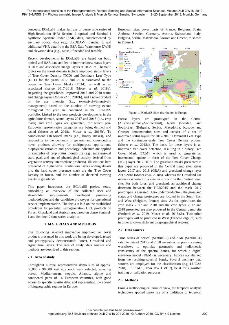
European sites cover parts of France, Belgium, Spain, Andorra, Sweden, Germany, Austria, Switzerland, Italy, Bulgaria, Serbia, Macedonia, Kosovo and Greece, as shown in Figure 1.

Figure 1. ECoLaSS Sites distribution in Europe

layersForest Centraltheinprototypedare

(Austria/Germany/Switzerland and(Sweden)North),

South-East (Bulgaria, Serbia, Macedonia, Kosovo and Greece) demonstration sites and consist of a set of improved status layers for 2017/2018: Dominant Leaf Type and the continuous-scale Tree Cover Density product

(Moser et al. 2018a). The basis for these layers is an improved tree cover detection, resulting in a binary Tree Cover Mask (TCM), which is used to generate an incremental update in form of the Tree Cover Change

(TCC) layer 2017-2018. The grassland masks presented in this paper are produced in the Central demo site: status layers 2017 and 2018 (GRA) and grassland change layer 2017-2018 (Moser et al. 2018b), whereas the Grassland use intensity is tested in a smaller site within the Central demo site. For both forest and grassland, an additional change detection between the HLR2015 and the mask 2017 prototypes is assessed. Also under production, the grassland status and change prototypes are located in the South-East and West (Belgium, France) sites. As for agriculture, the crop mask 2017 and 2018 and the crop types 2017 and 2018 presented are also produced in the Central demo site

(Probeck et al. 2019, Moser et al. 2018a,b). Two other prototypes will be produced in West (France/Belgium) sites

in order to cover different biogeographical regions.

2.2 Data sources

Time series of optical (Sentinel-2) and SAR (Sentinel-1)

satellite data of 2017 and 2018 are subject to pre-processing workflows to optimize geometric and radiometric consistency of the spectral bands, for which a digital elevation model (DEM) is necessary. Indices are derived from the resulting spectral bands. Several ancillary data sources are employed for the classification (e.g. LUCAS 2018, LPIS/IACS, ESA DWH VHR), be it for algorithm

training or validation purposes.

2.3 Methods

From a methodological point of view, the temporal analysis techniques applied make use of a multitude of temporal



202

https://www.ecolass.eu/test-prototype-sites

feature descriptors (multiple temporal statistical metrics). Temporal features describe distinct spectral, temporal and phenological properties. By selecting suitable time windows, the mapping of phenological transition points and phases is possible by simultaneously mitigation of cloud

cover issues within optical data.

2.3.1 Pre-processing:

In the case of optical data, atmospheric correction, topographic normalization and cloud and cloud shadow detection and masking are the key pre-processing steps. The ESA Sen2Cor package (Louis et al. 2016) and python scripts are used for this purpose. Cloud and cloud shadow masking embeds the generation of a binary mask, which is derived by a dedicated filtering and buffering process from the original Sen2Cor Scene Classification Layer (SCL). In the South-East demo site, the MACCS/MAJA cloud masking algorithm (Lounjou et al. 2016) is preferred in view of test performance outcomes. The topographic normalisation implemented in the Sen2Cor software uses a 90m DEM and creates slope, aspect and terrain shadow products. The output bands are resampled to 10 m using the cubic convolution method whereas the SCL is resampled using nearest neighbourhood. The three bands with 60 m spatial resolution (Bands 1, 9 and 10) are omitted in the Level-2A output. Topographic normalisation is performed to reduce illumination effects caused by certain topographic conditions and contributes to obtain a better consistency in the time series (e.g. sun angles and shadows dramatically vary throughout the seasons).

From the surface reflectance products, the following spectral indices are derived:

- NDVI (Normalized Difference Vegetation Index)

- NDWI (Normalized Difference Water Index)

- BRIGHTNESS (derived through summation of

the values of the bands Green, Red, NIR and

SWIR1)

- IRECI (Inverted Red-Edge Chlorophyll Index)

Together with the spectral information, these vegetation indices are the input for the subsequent thematic processing.

In turn, SAR time series are based on Level-1 products in Interferometric Wide swath (IW) mode and Level-1 Ground Range Detected (GRD). The pre-processing steps is performed with the ESA SNAP tool: orbit update (includes automatic precise orbits download), thermal noise removal, radiometric calibration generating a beta band, terrain flattening to gamma naught based on SRTM 1sec HGT, terrain correction using the same DEM generating a 10m resolution product and the export of the scene in DN units. After the orthorectification of the images, a multitemporal speckle filtering has been applied using a 5x5 Frost filter. Python scripts are used in indices derivation: VV (Gamma naught), VH (Gamma naught), Normalized Difference

VV/VH, Ratio VV/VH.

2.3.2 Temporal features computation:

Temporal feature descriptors are able to depict and quantify a surface’s status and its phenological behaviour over time as well as to capture the intensity and significance of

change information and time series related statistical properties. Thus, they constitute powerful input features for various classification or analysis tasks. Not being directly related to image acquisition dates, neither customised scene selection efforts nor prior knowledge of change event dates is required. Hence, feature descriptors can be flexibly computed from reflectance or derived index data.

For grassland, the time windows testing included the spring period (01.03-31.05), late winter to spring (01.01-01.06)

and a larger period (01.01-30.11). In the case of Forest, tests included several time windows (e.g., 15.03-15.06). The selected time windows for the TCM and DLT is related to the growing season (e.g., 15.03-15.09). In turn, the periods tested in Agriculture were selected to capture the crop season key moments (e.g., 15.03-15.10).

Seven temporal feature descriptors represent standard statistical temporal metrics of a time series: maximum, minimum, mean, median, standard deviation, covariance and and percentiles (10, 25, 50, 75, 90, difference 90-10 and difference 75-25).

In parallel to the new feature calculation and analysis, a feature selection method is applied. The K-Fold Cross Validation method is based on a stratified k fold sampling integrated in the machine learning package. This sampling method splits the training and test dataset into a number of k-folds. It clones the classifier in every iteration and produces accuracy figures and a new training and test set. The algorithm finally yields a combination of the features with the highest accuracy. This subset of features is used

for the classification process.

2.3.3 Classification:

Classification was applied using different combinations of sensor data and time periods to benchmark their respective feasibility, effort and accuracy: Sentinel-2, Sentinel-1, and the combination of Sentinel-1 and Sentinel-2 temporal features.

Two independent sample datasets were used for the classification and validation. In the case of forest and grasslands, samples were automatically extracted from a combined HRL 2015 sampling layer, consisting of the 20m Layers Dominant Leaf Type, Imperviousness, Grassland and Water and Wetness. In addition, LUCAS 2018 points filtered by the observation type 1 attribute and visually inspected if required, were also selected. To reduce the number of possible outliers and errors in these samples, the following filtering steps were applied to the sampling layer:

reduction of edge effects and mixed pixels through negative buffering (20 m) of the HRL product classes (e.g., coniferous forest, imperviousness, water) and removal of patches smaller than 1 ha. A stratified random point sampling has been performed within the remaining area. Subsequently, potential outliers have been removed by statistical analysis and visual checks, if required. For the agriculture crop mask and crop types, as no pre-existing HRL was available, LUCAS 2018 and LPIS data were respectively, employed for sampling purposes, following selection procedures as aforementioned. The sampling set is split into the set used for training purposes and the



203

validation independent sample set, in a 50%-50% proportion.

Using a random forest-based classification approach on several hundred temporal feature descriptors, a feature selection is performed to identify the most meaningful input features for classification, ensuring a high resultant product quality as well as a cost and time efficient processing with high accuracy. A probability layer indicating the percentage of reliability constitutes a pixel-based quality indicator by- product.

In the case of the intensity layer, NDVI time series are used to derive the number of mowing events, that are clipped to the grassland mask and reclassified by defining the extensive use category when less than or equal to 2 mowing events are detected during the year.

A final post-classification filtering was based on a five minimum pixel count of connected patches (e.g., GRA as well as non-GRA), and case-wise application of elevation thresholds (e.g., Agriculture > 1700 m threshold). All patches smaller than five pixels (i.e., minimum mapping unit 5 pixels) were removed to close holes in grassland patches and remove very small patches.

Consistent with the TCM & DLT, a continuous-scale Tree Cover Density product with values ranging from 0-100% is produced at 10m spatial resolution using band-specific temporal features from Sentinel-2 and a multiple linear regression estimator. The pixel-based TCD product provides information on the proportional crown coverage per pixel in percent, whereas tree cover density is defined as the „vertical projection of tree crowns to a horizontal earth’s surface“. Two different approaches have been used to generate the status layer Tree Cover Density 2018 using a linear regression estimator: a mono-temporal classification using a “best-of” scene approach and a multi- temporal classification using band-specific temporal features for defined time windows. The latter one shows very promising results and is recommended for an

operational roll-out on European level.

2.3.4 Change detection:

In view of a potential future HRL Forest Incremental Update layer, the delineation of forest change/loss is based on the comparison of a pre- and post-change tree cover mask (map-to-map change approach with subsequent MMU filtering, followed by a NDVI plausibility analysis of detected changes. The Incremental Update layer resulting thereof, hereinafter explicitly named as Tree Cover Change

(TCC), compares the pre- and post-change mask (TCM 2017 and TCM 2018) to detect areas of change with a minimum mapping unit of 1 ha. Due to the very short time interval of mostly < 1 year between the two masks, this layer concentrates on negative changes (loss) only. The methodology incorporates both, Sentinel-1 and Sentinel-2 data and provides more flexibility in areas of frequent cloud cover. This combination of a map-to-map comparison and change indicators derived from Sentinel-2 time series (e.g., minimum NDVI differences) of both years provides a more robust change detection than a common map-to-map change approach. The approach has been also applied

(slightly modified) to the grassland change.

2.3.5 Validation and benchmarking:

A statistical validation is carried out on the basis of a stratified systematic sampling approach with area-weighted accuracy calculation. Unequal sampling intensity resulting from the stratified systematic sampling approach is accounted for by applying a weighting factor to each sample unit based on the ratio between the number of samples and the size of the stratum considered. The weighing factor is inversely proportional to the inclusion probability (i.e., the probability that a pixel will be included in the sample) of samples from a given stratum. Within a geographic stratum, the inclusion probabilities of all sample units are equal. To combine sample data over several strata, a weighted estimator of the error matrix is required to account for the different inclusion probabilities among strata. The estimation weight is the inverse of each sample unit´s inclusion probability, and the proportion of area for each cell of the error matrix is estimated. Else, true map accuracies might result over or under estimated. Overall accuracy and class specific accuracies (user and producer accuracy) are computed for all thematic classes from the weighted sampling probability-corrected confusion matrix Ci,j (for points classified into class i and validated in class j), and 95% confidence intervals are calculated for each accuracy. From these, the F1 score statistic is computed per class for the status layers and change layers, as the harmonic mean between precision (i.e., User accuracy) and recall (i.e., producer accuracy), where an F1 score reaches its best value at 1 (perfect precision and recall) and worst at 0. In case of the TCD, the regression goodness-of-fit statistics are computed (i,e, i,e, Mean Absolute Error MAE, Root Mean Square Error RMSE and the coefficient of

2dtermination R ). The layers are also assessed qualitatively

by visual inspection using VHR data.

3. RESULTS AND DISCUSSION

The overall thematic accuracies for all Grassland, Forest, and Arable Land layer prototype implementations produced so far are promising, ranging from 77-98%. The lessons- learned from the first temporal feature descriptors extraction and selection tests, together with the added value of the combined use of both optical and radar data, lead

now to refined workflows and results.

3.1 Forest products

To derive the 2018 TCM and DLT, in total, 234 features were available to feed the machine learning algorithm: 182 features for the Sentinel-2 indices and bands, and 52 features from the Sentinel-1 single bands and indices. SAR temporal features derived from the VH polarisation (e.g. VH_p025, VH_p010) turned out to have a high importance in the tree cover detection followed by features derived from the Sentinel-2 bands B02 and B03 as well as NDVI and NDWI features. With respect to the DLT classification, SAR features show no benefit for the leaf type discrimination. Here, band-specific features from Sentinel- 2 dominate clearly over all other derived features. Worth mentioning is the dominance of features derived from the SWIR bands (B11, B12). A significant influence of the feature selection method on the overall accuracy figures

(retrieved by LUCAS 2018 points) could not be observed.



204

Increasing the spring time window (15.03-15.06) to the

extent of the whole growing season period (15.03-15.09) is

drastically increasing the data volume and processing time

(and logically also the production costs) but has a positive

effect on the achieved overall accuracy of the TCM, which

is in the magnitude of 2 to 4 percentage points. This is

mainly due to the increased data availability and a

potentially higher rate of data acquisitions without or with

less cloud cover. However, the strongest influence on

classification accuracies can be observed by the quality of

the samples. A subsequently performed validation with 800

LUCAS 2018 points confirmed very high overall

accuracies for both, the TCM as well as the DLT

classification (98% OA and 93% OA respectively in the

Central demo site).

In order to generate a comparable and future-oriented data

basis for the incremental update, the same feature and

sample sets have been used to derive improved TCMs and

DLT layer for the reference year 2017. Then, the

incremental update layer TCC 2017-2018 has been

produced following a map-to-map change approach,

leading to an improved geometric and thematic accuracy of

the derived changes (forest loss).

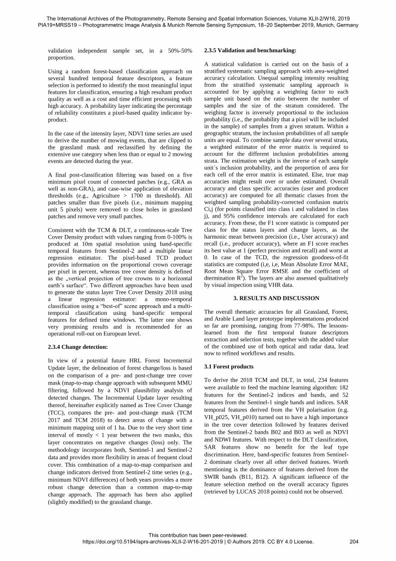
The continuous Tree Cover Density product 2018 (Figure

2) adds unprecedented detail to the binary Tree Cover

Mask. For the TCD, the mean and median features from the

spectral Sentinel-2 bands provide promising results. Both

classification approaches tested in the forest status layers

rendered similar results (best-of-scene and mono-temporal),

although in the end the multi-temporal classification using

band-specific temporal features for the defined time

windows was selected. The goodness-of-fit statistics for the

linear regression model of the TCD 2018 obtained are: 7.65

MAE, 8.14 RMSE, and 0.93 R2.

Figure 2. Multi-temporal S-2 feature stack (upper figure) and

the derived TCD 2018

3.2 Grassland products

With the availability of dense optical and SAR time series from Sentinel-1 and Sentinel-2, grassland mapping can profit from the increased information content provided by temporal measurements of the reflectance of grassland areas over the year. Based on reinterpreted LUCAS samples a supervised classification approach using the Random Forest classifier has been successfully applied.

The feature selection tests automatically executed by the Random Classifier have shown that, in the Central demo site, best performing input indices are NDVI, NDWI, IRECI and Brightness. Regarding SAR data generally the following annual coefficients have shown the best performance: VH polarisation, the VV polarisation and the NDVVVH Ratio.

The later winter to spring (January to June) time window in the end did not bring an added value for classification. In different biogeographical regions the short time window can differ (which is also the case in the forest and agriculture products). To better match the local conditions, it is important to define a time window where grassland and cropland (class generating most misclassifications) are best separable (e.g., define the period when grassland is already greening whilst cropland is not). In Mediterranean regions, for instance, this window may be shifted more towards winter (e.g. Dec-Mar).

After the visual interpretation of all classifications, it can be observed that using optical data only more confusion between grasslands and cropland are present, whereas using SAR data only more misclassifications between grassland and roads are present. The combined approach shows more homogenous patches than using SAR data only, diminishing confusion with other classes suchlike tree cover and plantations, that otherwise cannot be excluded when using only S-2. This is relevant as in fact the overall accuracy values obtained are misleading while the visual inspection demonstrates the combined approach performs best. A main requirement however is the precise pre- processing of the dense time series including a topographic normalisation for hilly to mountainous terrain. For SAR time-series the application of multi-temporal filtering on gamma naught corrected imagery is recommended

For the Central site Grassland mask 2018, the overall accuracy is 96.6% (0.93% Confidence Interval), producer accuracy is 91.0% and user accuracy 90.5%.

Regarding the change layers, as only the geometrical change areas are shown and no further exclusion of non- change by the usage of e.g. NDVI minimum or other change indicators is applied to the 2017-2015 change layer, there are many more changes visible compared to the 2017/18 change layer. Most of them in truth are no real change, instead resulting from weaknesses in the 2015 layer.

In areas of higher elevation and where snow cover is found for long periods of the year in the South of the demo site, the classification is not that accurate for both years (2015 & 2018) which in turn leads to greater differences and



205

therefore change detection which is basically no change.

An elevation threshold was applied to reduce such errors,

which significantly improved the respective grassland

masks in the most problematic regions. Filtering

significantly contributes to keep meaningful changes while

removing small areas, likely classification errors. All areas

below 1 ha (25 pixels) were filtered.

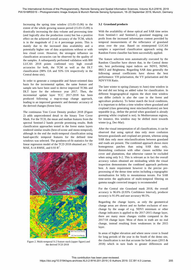
The figure below shows a detail of the grassland intensity

2018 layer, consistent as derived from the areas defined as

grassland within the grassland status layer, and based on a

simple although effective NDVI time series analysis, with a

good trade-off between computer resources and

preprocessing timing (i.e., impact in updates production

timeliness) and achieved thematic accuracy. The datasets

used for validation for the use intensity grassland product

are the IACS/LPIS, generating an overall accuracy of

81.5%.

Figure 3. Grassland intensity layer 2018 (upper figure)

compared to Bing Maps Aerial of the same region

The current temporal density of optical time-series from Sentinel-2 for the years 2017 and 2016 restricted the applicability of time series methods, as reflectance trajectories depend on the grassland dynamics over the vegetation period such as e.g. mowing events. The high cloud coverage in 2018 in central Europe limits the method of comparing NDVIs of consecutive acquisition dates:

mowing events may not be detected in areas covered by clouds for long periods. Filtering improved look and feel by reducing noise. For the use intensity layer, a filter of 4 pixels in size was applied. All areas within the grassland mask where filtered, so that there are no intensity classes smaller than 5 pixels in the end. Within small grassland

patches, it might happen that e.g. three pixels are categorized as extensive and two are intensive. In such cases, the filter would cause the class values to jump between classes with each filter iteration without getting a patch of five unique values. If so, the patch was filtered in favour of intensive use because most of the areas are used

intensively in the demo site.

3.3 Agriculture Products

The time interval algorithms are strongly affected by undetected clouds/cloud shadows as well as confusion with bright surfaces in the cloud mask. These algorithms present many artefacts and data gaps due to the short compositing period and the interval between images available in the time series. To avoid potential artefacts derived from the presence of unmasked cloud cover pixels, time periods were selected to guarantee a sufficient number of imagery to minimize the distortion that extreme values would pose to the statistics.

Concerning Agriculture classification an initial set of criteria to evaluate the best compositing method for crop recognition (cropland-CL, crop type-CT) and crop growth monitoring (CG) have been selected. The benchmark is performed on Central (Germany) and Belgium site and show promising accuracies and high potential of time series and derived temporal features for crop mask extraction and crop type monitoring. As is not uncommon in agriculture products, the local conditions (e.g., climate, soil, altitude, topography, crop phenology) influencing this specific land cover makes it a challenge to target a HRL at a continental scale. In our case, stratification was applied for a better adaptation to the particularities of the different subregions within the Central demo site.

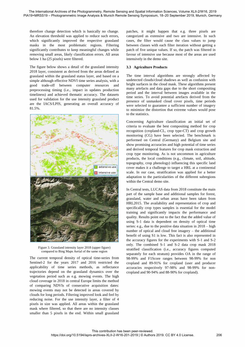
In Central tests, LUCAS data from 2018 constitute the main part of the sample base and additional samples for forest, grassland, water and urban areas have been taken from HRL2015. The availability and representation of crop and specifically crop types samples is essential for the model training and significantly impacts the performance and quality. Results point out to the fact that the added value of using S-1 data is dependent on density of optical time series: e.g., due to the positive data situation in 2018 – high number of optical and cloud free imagery – the additional benefit of using S1 is low. This fact is also represented in the accuracy figures for the experiments with S-1 and S-2 only. The combined S-1 and S-2 data crop mask 2018 stratified classification (i.e., accuracy figures computed separately for each stratum) provides OA in the range of 98-99% and F1Score ranges between 98-99% for non cropland and 89-91% for cropland (user and producer accuracies respectively 97-98% and 98-99% for non- cropland and 90-94% and 88-90% for cropland).



206

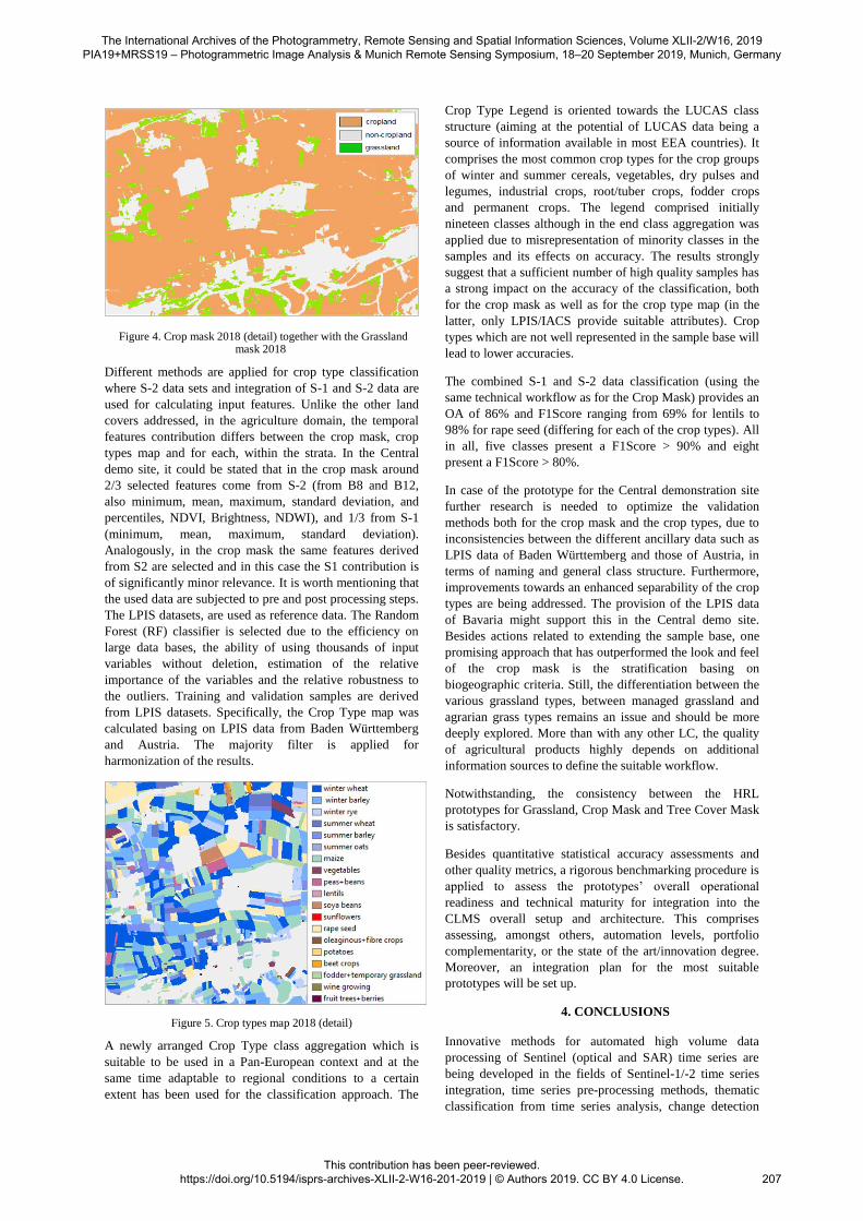
Figure 4. Crop mask 2018 (detail) together with the Grasslandmask 2018

Different methods are applied for crop type classification

where S-2 data sets and integration of S-1 and S-2 data are

used for calculating input features. Unlike the other land

covers addressed, in the agriculture domain, the temporal

features contribution differs between the crop mask, crop

types map and for each, within the strata. In the Central

demo site, it could be stated that in the crop mask around

2/3 selected features come from S-2 (from B8 and B12,

also minimum, mean, maximum, standard deviation, and

percentiles, NDVI, Brightness, NDWI), and 1/3 from S-1

(minimum, mean, maximum, standard deviation).

Analogously, in the crop mask the same features derived

from S2 are selected and in this case the S1 contribution is

of significantly minor relevance. It is worth mentioning that

the used data are subjected to pre and post processing steps.

The LPIS datasets, are used as reference data. The Random

Forest (RF) classifier is selected due to the efficiency on

large data bases, the ability of using thousands of input

variables without deletion, estimation of the relative

importance of the variables and the relative robustness to

the outliers. Training and validation samples are derived

from LPIS datasets. Specifically, the Crop Type map was

calculated basing on LPIS data from Baden Württemberg

and Austria. The majority filter is applied for

harmonization of the results.

Figure 5. Crop types map 2018 (detail)

A newly arranged Crop Type class aggregation which is suitable to be used in a Pan-European context and at the same time adaptable to regional conditions to a certain extent has been used for the classification approach. The

Crop Type Legend is oriented towards the LUCAS class structure (aiming at the potential of LUCAS data being a source of information available in most EEA countries). It comprises the most common crop types for the crop groups of winter and summer cereals, vegetables, dry pulses and legumes, industrial crops, root/tuber crops, fodder crops and permanent crops. The legend comprised initially nineteen classes although in the end class aggregation was applied due to misrepresentation of minority classes in the samples and its effects on accuracy. The results strongly suggest that a sufficient number of high quality samples has a strong impact on the accuracy of the classification, both for the crop mask as well as for the crop type map (in the latter, only LPIS/IACS provide suitable attributes). Crop types which are not well represented in the sample base will lead to lower accuracies.

The combined S-1 and S-2 data classification (using the same technical workflow as for the Crop Mask) provides an OA of 86% and F1Score ranging from 69% for lentils to 98% for rape seed (differing for each of the crop types). All in all, five classes present a F1Score > 90% and eight present a F1Score > 80%.

In case of the prototype for the Central demonstration site further research is needed to optimize the validation methods both for the crop mask and the crop types, due to inconsistencies between the different ancillary data such as LPIS data of Baden Württemberg and those of Austria, in terms of naming and general class structure. Furthermore, improvements towards an enhanced separability of the crop types are being addressed. The provision of the LPIS data of Bavaria might support this in the Central demo site. Besides actions related to extending the sample base, one promising approach that has outperformed the look and feel of the crop mask is the stratification basing on biogeographic criteria. Still, the differentiation between the various grassland types, between managed grassland and agrarian grass types remains an issue and should be more deeply explored. More than with any other LC, the quality of agricultural products highly depends on additional information sources to define the suitable workflow.

Notwithstanding, the consistency between the HRL prototypes for Grassland, Crop Mask and Tree Cover Mask is satisfactory.

Besides quantitative statistical accuracy assessments and other quality metrics, a rigorous benchmarking procedure is applied to assess the prototypes’ overall operational readiness and technical maturity for integration into the CLMS overall setup and architecture. This comprises assessing, amongst others, automation levels, portfolio complementarity, or the state of the art/innovation degree. Moreover, an integration plan for the most suitable

prototypes will be set up.

4. CONCLUSIONS

Innovative methods for automated high volume data processing of Sentinel (optical and SAR) time series are being developed in the fields of Sentinel-1/-2 time series integration, time series pre-processing methods, thematic classification from time series analysis, change detection



207

from time series analysis and incremental update

methodologies for the Copernicus Land High Resolution

Layers (HRLs).

With regards to accuracy, in addition to the time windows

selection for time features computation, sampling is key. In

ECoLaSS, a multi-stage sampling approach has been

applied: automatic reference sampling based on a sampling

layer generated from the HRLs 2015, outlier detection with

visual/statistical validation of the samples and split of the

sample dataset into training and validation dataset, initial

classification and re-sampling based on an analysis of

omission and commission errors with subsequent iteration

loops.

Iterative calculation over a time stack allows for

implementing suitable dynamic change detection systems,

which require to be frequently updated, such as it would be

the case for the existing HRL forest and grassland services

as well as for a potential future arable land service. The

change layer products quality is totally relying on the

quality of the respective status layers. The probability

layers for each of the status products from which the

change is assessed by indicating the pixel level accuracy

confidence and the expert knowledge are relevant in a

suitable production workflow for a comprehensive change

detection.

The improvement endeavours of existing products comprise

assessing prototypes of enhanced tree cover, leaf types, tree

cover density within, and tree cover change layers as yearly

updates, as well as better-quality permanent grassland

classification and use categorisation together with a yearly

change identification approach. The production of an

Incremental Update Layer for the Forest HRL and its roll-

out on European level has been rated as feasible.

Entirely novel products are targeted, such as a possible

future HRL on arable land, for which a prototype is

presented, targeting a pan-European crop mask of high

precision and a representative, robust classification of crop

types.

The prototype of the new agriculture service shows that the

definition of a pan-European crop-types legend is not

straightforward, as crop phenology follows rather regional

and local scale patterns and not all classes are present at the

continental scale. In addition, the availability of a sufficient

number of high quality samples is essential to obtain

reliable crop masks and crop types products within. The

demo site in Central Europe proves that a locally-adapted

stratification accounting for biogeographic heterogeneity

(i.e., climate, soil, altitude) highly reduced

misclassifications for both agricultural products.

In ECoLaSS, these and all other candidate prototypes are being produced with a view to a potential pan-European for service roll-out. For the most promising prototypes a detailed integration plan into the Copernicus service

architecture is being developed.

REFERENCES

Lonjou, V., Desjardins, C., Hagolle, O., Petrucci, B., Tremas, T., Dejus, M., Makarau, A., Auer, S., 2016. MACCS-ATCOR joint algorithm (MAJA). Presented at the Remote Sensing of Clouds and the Atmosphere XXI, International Society for Optics and Photonics,

1000107.

Louis, J., Debaecker, V., Pflug, B., Main-Knorn, M., Bieniarz, J., Mueller-Wilm, U., Cadau, E., Gascon, F., 2016. Sentinel-2 Level-2 Processor Sen2Cor.

Moser, L., Probeck, M., Ramminger, G., Rieke, C., Mack, B., Ickerott, M., Storch, C., Sommer, C., Richter, R., Herrmann, D., Ruiz, I., Kovatsch, M., and Schwab K.

(2018a): Evolution of Next-generation Copernicus High

Resolution Layers on Forest and Agriculture: TherdECoLaSS Project. 3 joint EARSeL LCLU & NASA

LCLUC Workshop (11-12 July 2018 in Chania, Greece)

Moser, L., Probeck, M., Ramminger, G., Richter, R., Herrmann, D. (2018b): Sentinel Time Series for Next- generation Copernicus High Resolution Layers on Agriculture and Grassland. INSPIRE Conference (18-21 September 2018 in Antwerp, Belgium)

Probeck, M., Schwab, K., Sevillano Marco, E., Herrmann, D., Sandow, C., Richter, R., Moser, L.: Prototypes of Future Copernicus Land Monitoring Products: The ECoLaSS Project. ESA Living Planet Symposium (13.-17.

May 2019, Milano, Italy)

ACKNOWLEDGEMENTS

The research leading to these results has received funding from the European Union’s Horizon 2020 Research and Innovation Programme, under Grant Agreement no 73000. The content of this paper does not reflect the official opinion of the European Union. Responsibility for the information and views expressed therein lies entirely with the author(s). The study used Copernicus Land Monitoring Service products © European Union, CLMS 2018, European Environment Agency (EEA). We acknowledge the use of LPIS data provided by the agricultural ministry of Baden-Württemberg and LUCAS 2018 provided by the European Commission/EUROSTAT.



208

http://worldcover2017.esa.int/



Documents

IMPRO EMENT OF EXISTING AND DE ELOPMENT OF FUTURE …...Copernicus Land Monitoring Service, ECoLaSS, Earth Observation, DIAS, HRL, LCLU, Sentinel, time. series analysis. ABSTRACT: