Embed Size (px)
Citation preview
Alma Mater Studiorum – Università di Bologna
DOTTORATO DI RICERCA IN
Ingegneria Elettronica, Informatica e delle Telecomunicazioni
Ciclo XXVII
Settore Concorsuale di afferenza: 09/F2 Settore Scientifico disciplinare: ING-INF/03
GNSS Interference Management Techniques
Against Malicious Attacks
Presentata da: Roberta Casile
Coordinatore Dottorato Relatore Prof. Alessandro Vanelli Coralli
Prof. Giovanni Emanuele Corazza
Esame finale anno 2015

roberta casile
G N S S I N T E R F E R E N C E M A N A G E M E N TT E C H N I Q U E S
A G A I N S T M A L I C I O U S AT TA C K SPh.D. Programme in Electronics Engineering, Telecommunications
and Information Technology - XXVII CycleDepartment of Electrical, Electronic and Information Engineering -
DEIAlma Mater Studiorum - Università di Bologna

G N S S I N T E R F E R E N C E M A N A G E M E N T T E C H N I Q U E SA G A I N S T M A L I C I O U S AT TA C K S
roberta casile
Ph.D. Programme in Electronics Engineering, Telecommunications and InformationTechnology - XXVII Cycle
Coordinator: Prof. Alessandro Vanelli-CoralliSupervisor: Prof. Giovanni E. Corazza
SC: 09/F2
SSD: ING-INF/03
Department of Electrical, Electronic and Information Engineering - DEIAlma Mater Studiorum - Università di Bologna
March 2015
Roberta Casile: , Department of Electrical, Electronic and InformationEngineering - DEI, Alma Mater Studiorum - Università di Bologna, ©March 2015

To strive, to seek, to find, and not to yield.
— Alfred Tennyson, Ulysses

A B S T R A C T
This thesis collects the outcomes of a Ph.D. course in Telecommuni-cations Engineering and it is focused on the study and design of pos-sible techniques able to counteract interference signal in Global Nav-igation Satellite System (GNSS) systems. The subject is the jammingthreat in navigation systems, that has become a very increasingly im-portant topic in recent years, due to the wide diffusion of GNSS-basedcivil applications. Detection and mitigation techniques are developedin order to fight out jamming signals, tested in different scenarios andincluding sophisticated signals. The thesis is organized in two mainparts, which deal with management of GNSS intentional counterfeitsignals.
The first part deals with the interference management, focusing onthe intentional interfering signal. In particular, a technique for thedetection and localization of the interfering signal level in the GNSS
bands in frequency domain has been proposed. In addition, an effec-tive mitigation technique which exploits the periodic characteristicsof the common jamming signals reducing interfering effects at thereceiver side has been introduced. Moreover, this technique has beenalso tested in a different and more complicated scenario resulting stilleffective in mitigation and cancellation the interfering signal, withouthigh complexity.
The second part still deals with the problem of interference man-agement, but regarding with more sophisticated signal. The attentionis focused on the detection of spoofing signal, which is the most com-plex among the jamming signal types. Due to this highly difficulty indetect and mitigate this kind of signal, spoofing threat is consideredthe most dangerous. In this work, a possible techniques able to detectthis sophisticated signal has been proposed, observing and exploitingjointly the outputs of several operational block measurements of theGNSS receiver operating chain.
vii

I N T R O D U C T I O N
Nowadays, the major part of the people worldwide relies on satellitenavigation systems to provide Position-Velocity-Time (PVT) solutionsto a number of critical and commercial applications, with a strongimpact on most aspects of the daily human life and for the societytoo. All common devices used everyday, as smartphones and vehicles,have a GNSS receiver, thus several applications rely on the accuracyof the delivered PVT solutions. In addition, the civilian applicationsthat range from emergency to route instructions, including also allthe types of transportation systems, from air through marine to land,and police and rescue services and many more, are based on the effi-cient functionalities of the GNSS infrastructure and thus they dependon the correct and reliable geosecurity location information. As a con-sequence of this growing demand, as a resource becomes spread anduseful among civil infrastructure, malicious agents attempt to disruptthe GNSS services exploiting possible weakness inside the target sys-tem.
interference in gnss
The widespread use of civil location-based applications is due to theGlobal Positioning System (GPS), and more in general GNSS, signalstructure which is defined in a freely-available and open-access spec-ification [24][72]. Due to the low received power at earth’s surface,GNSS signals are highly vulnerable to the most common attack asdenial-of-service by jamming and intentional interference, which canbe effective also within a range of several kilometers. The GNSS ser-vice deterioration is the result of natural disruptions, as ionosphericand tropospheric effects, unintentional artificial effects, as multipath,deliberate,intentional and malicious artificial effects, as jamming, mea-coning and spoofing signals. In order to limit these deteriorating ef-fects, it is necessary to design techniques against interfering signaldue to the increasing diffusion of the GNSS based applications. Sev-eral types of interfering signals can affect GNSS operation in a differ-ent manner and a main characterization in different groups can bemade. Thus, navigation system interfering signal can be divided inintentional and unintentional, and thus in jamming and out of bandsignals, respectively.
Unintentional
GNSS services can be deteriorated by Radio Frequency Interference(RFI) generated by instruments that are not working properly. Thiselectronics elements can deny the service of navigation systems gen-erating out-of-band frequencies that fall into the GNSS bands [83]. In
ix
[15] the attention has been focused on the effects of the Digital VideoBroadcast - Terrestrial (DVB-T) standard in the GNSS system. Authorshave studied and show that due to the large diffusion of the receiverequipments for DVB-T system, this type of unintentional interfererrepresents an important issue to be solved also because the corre-sponding transmitters emit signals with a very close frequency toGNSS band, causing a high interference level. However, harmonic sup-pression capabilities of the antennas can reduce the effect of this kindof interference. Moving from electronic devices, the more dangerousnon-intentional interfering signal occurs when the correct signal is af-fected by multipath propagation. When a GNSS receiver is located ina worse scenario as a urban canyon and it is not in Line of Sight (LOS),its functionalities are highly corrupted due to the several delayedreplicas that are received, generated by the reflection of the usefulsignal on obstacles surfaces surrounding the receiver. These delayedreplicas reduce the capabilities of the receiver in decoding and evalu-ating the PVT solutions (the shape of the correlation peak is distorted)and thus deteriorating the reception of the signal.
Intentional
The other main category is represented by the intentional interferer.These signal are generated to deny intentionally services providedby GNSS system. The scope of the jammer is to completely destroythe communication between transmitter and receiver and to deny thepossibility of a correct exchange of information, and thus to receivePVT solutions (especially in military domain). Several possible strate-gies can be implemented by a jammer in order to be effective, and itdepends on the type of target to be jammed. Usually, jamming wave-forms are modulated signals as continuous wave, pulsed continuouswave, chirp signal. Electronic devices able to generate this jammingwaveform can be purchased on-line at a very low cost, thus beingavailable to be easily used. This Personal Privacy Device (PPD)s evenif generating a low power signal, can deny the correct reception to thetarget and also to the closer receiver in a radius of less meters [31].Among intentional interferer, also meaconing and spoofing signalshave to be considered. These signals belong to the category of struc-tured interferer with the main scope to mislead the GNSS sending to ita wrong PVT information, without any awareness by the receiver. Mea-coning signal refer to the reception and the rebroadcast of the GNSS
signal aiming to confuse with a wrong time-alignment the target re-ceiver. Usually, meaconing is generated using a low noise amplifierand two passive antennas, without any navigation processor. On theother hand, spoofer represents the counterfeit copy of the GNSS signal.Among spoofer it is possible to discern simplistic spoofer, intermedi-ate spoofer and sophisticated one. The first type is generated by aGPS generator and a transmitting antenna. It is very easy to detectsimplistic spoofer signals because they are not able to duplicate or re-produce the correct time-synchronization of the GNSS signal-in-space.
x
The other types of spoofer signal are more complex. The intermedi-ate and sophisticated spoofer is able to generate a malicious signalthat it is totally equal to the useful one. This jammer source can cor-rectly estimate the right time-synchronization of the constellation inview and consequently the receiver acquires and tracks this counter-feit copy without knowing that a malicious attack is occurring. Inother words, under a spoofing or meaconing attack, a GNSS receiveris providing PVT solutions with good signal quality measures evenif the position solutions do not represent the actual location of thereceiver.
motivation
Taking into account this ever-growing dependance on GNSS, due tothe several civil and safety existing applications, strong motivationto attack civil GNSS infrastructure has increased, for either an illegit-imate advantage or terrorism purposes. Due to the known structureof the GNSS signal and for a non in-built security feature in the GNSS
open service, the design of a jamming source able to deteriorate thecorrect operational function is becoming more feasible thanks to thevery low cost of the necessary equipment [36]. Consequently, all jam-ming events and in particular the spoofer are becoming a serious is-sue for the next-generation of the GNSS infrastructure, and techniquescapable to counteract these malicious attacks are required. The prin-cipal problem is strictly correlated to the huge diversification of theGNSS receivers; in other words, it is necessary to design detection andmitigation methods that do not require big hardware modifications.So far, several methods have been proposed to harden civil GNSS re-ceiver against jamming attacks and in particular against spoofing ef-fects. But in any case, civilian GNSS infrastructure is still subjectedand without any defense solution against this sophisticated attack.
conclusion
In summary, GNSS interference management research topic still presentsopen challenge due to the wide application arena and to the growingtechnological developments. In this dissertation the results of the re-search carried out during my Ph.D. activity are presented, in the con-text of structured interference management for satellite navigationsystems. This activity has been mainly characterized by the continu-ous interaction with industrial partners within the framework of inter-national research project [Pr1]. All the results of my activity providedin this dissertation represent possible solutions to the problems en-countered within the aforementioned project. The collaboration andinteraction with industrial partners have lead to a deeper comprehen-sion of the requirement and of the trade-offs due to practical imple-mentation. This opportunity has allowed to test the provided tech-
xi
niques with real data collected in a controlled scenario, satisfying thepractical requirements.
O R I G I N A L C O N T R I B U T I O N S
In this dissertation, the effects of interfering signal in satellite naviga-tion systems have been studied and analyzed. Possible and innovativetechniques are provided with the aim of reduction of the jamming ef-fects and thus to enhance the reliability and the functionality of theGNSS receiver. It is worthwhile to underline that the scope of the thesisis then trying to detect interferers and collect malicious signals fromthe very statistical point of view taking into account that the GNSS
receiver aims to mitigate interfering effects rather than to detect it.This consideration allows to deal with detection and characterizationof even very low-power jammers. The principal contribution of thethesis regards with the jamming management technique in complexscenarios. In the framework of the DETECTOR project [Pr1] a deepdescription and overview of the interfering issue in satellite naviga-tion systems has been carried out. Considering the main purpose ofthe project, the PhD candidate has described and provided new ap-proaches in detection and mitigation of jamming signals. In particular,moving from scientistic previous references, interfering signal withparticular characteristics have been considered, evaluated from ex-haustive measurement campaigns. From these results, an innovativeapproach for the detection and above all for the mitigation of interfer-ing signals has been designed [P4]. Moreover, a development of thestudy-case is provided. The aforementioned detection and mitigationtechniques has been tested in a different scenarios, worse than theprevious one. The innovative aspect consists in the possibility of ap-ply the already described methods to more complex scenario, as canbe the dispersive channel, and verify that they still properly work. Inother words, in this dissertation a general study of the interfering sig-nal in a multipath scenario (urban canyon) is provided and numericalresults show that provided technique is still effective in detecting andcanceling the jamming waveform, with a slightly decreased perfor-mance but without any increasing of the computational complexityof the solution in [P4]. Furthermore, the attention has been focusedon a more sophisticated class of jamming signal, i. e.the spoofer. It iswell known that spoofing signals represent the most difficult kind ofsignal to be detected and consequently to be mitigated. In the disserta-tion, a possible and innovative approach is presented. This techniqueis based on the jointly observation and evaluation of measurementoutputs from several blocks locating inside GNSS receiver. Throughthese measurements, it is possible to define threshold in order to de-tect the spoofer when it occurs. The results have been carried out byobserving real data collected in controlled scenario with different im-
xii
plementation and by evaluation from real-space GNSS signal collectedin airport station.
P E R S O N A L P U B L I C AT I O N S
[P1] Bartolucci, M; Casile, R.; Pojani, G.; Corazza, G.E.;, “Joint Jam-mer Detection and Localization for Dependable GNSS," Position-ing, Navigation and Timing (ION-PNT), 2015 International Confer-ence on, April 2015 (SUBMITTED TO).
[P2] Bartolucci, M; Casile, R.; Gabelli, G.; Guidotti, A.; Corazza, G.E.;“Distributed-Sensing Waveform Estimation for Interference Can-cellation," Proceedings of the 27th International Technical Meeting ofthe Satellite Division of The Institute of Navigation (ION GNSS+2014), September 2014.
[P3] Bartolucci, M; Casile, R.; Corazza, G.E.; Durante, A.; Gabelli,G.;Guidotti, A.;, “Cooperativedistributed localization and char-acterization of GNSS jamming interference," Localization and GNSS(ICL-GNSS), 2013 International Conference on, June 2013.
[P4] Gabelli, G.; Casile, R.; Guidotti, A.; Corazza, G.E.; “GNSS Jam-ming Interference: Characterization and Cancellation," Proceed-ings of the 2013 International Technical Meeting of The Institute ofNavigation, January 2013.
[P5] Gabelli, G.; Corazza, G.E.; Deambrogio, L.; Casile, R.; , “Code ac-quisition under strong dynamics: The case of TT&C for LEOP,"Advanced Satellite Multimedia Systems Conference (ASMS) and 12thSignal Processing for Space Communications Workshop (SPSC), 2012.
P R O J E C T S
[Pr1] “Detection, Evaluation and Characterization of Threats to RoadApplications (DETECTOR)," FP7 Grant Agreement: 277619-2 -in collaboration with Nottingham Scientific Limited (NSL), SANEF,ARIC, Black Holes B.V. and IPSC.
xiii

C O N T E N T S
i interference management techniques 1
1 interference detection 3
1.1 Introduction 3
1.2 System Model 4
1.3 Interference Band Detection 5
1.3.1 Performance Analysis 7
1.4 Interference Duty-Cycle Estimation 12
1.4.1 Duty-Cycle Estimation 13
1.4.2 Performance Analysis 16
1.5 Bandwidth Detection: Update and Validation 19
1.5.1 Bandwidth Detection Algorithm: Update Descrip-tion 21
1.5.2 Bandwidth Detection: Validation Campaign 24
1.6 Conclusions 45
2 gnss jammer in multipath scenario 47
2.1 Introduction 47
2.2 System Model 48
2.3 Algorithm Description 49
2.3.1 Interferer Detection 50
2.3.2 Interferer Waveform Acquisition 54
2.3.3 Interferer Waveform Estimation 54
2.3.4 Interferer Waveform Mitigation 55
2.3.5 Complexity Evaluation 56
2.4 Non-dispersive Channel 58
2.4.1 Jamming Chirp 59
2.4.2 Jamming Chirp Autocorrelation Analysis 59
2.4.3 Numerical Results 62
2.4.4 Complexity Evaluation 71
2.5 Multipath Channel 72
2.5.1 System model 73
2.5.2 Autocorrelation Analysis 74
2.5.3 Detector Design 76
2.5.4 Numerical Results 78
2.5.5 Complexity Evaluation 89
2.6 Conclusions 91
ii spoofing threat 99
3 spoofing in gnss 101
3.1 Introduction 101
3.2 Literature Survey 102
3.3 Spoofing Detection: Signal Quality Monitoring techniques 105
3.4 Proposed Architecture 106
3.4.1 System model 107
3.4.2 Automatic Gain Control 107
3.4.3 Correlator 109
xv
xvi contents
3.4.4 C/N0 estimation 109
3.4.5 AGC & Correlator & C/N0 : A combined Tech-nique 110
3.5 Numerical Results 111
3.5.1 Scenario 111
3.5.2 Simulation Results 111
3.6 Conclusions 123
bibliography 131
L I S T O F F I G U R E S
Figure 1 Band Detection - Block Diagram 6
Figure 2 Pmd,Pout@ Observation duration equal to 10[µs]and fmax = 8[MHz] 9
Figure 3 Pmd,Pout@ Observation duration equal to 10[µs]and fmax = 4[MHz] 10
Figure 4 Pmd,Pout@ Observation duration equal to 10[µs]and fmax = 2[MHz] 10
Figure 5 Pmd,Pout@ Observation duration equal to 10[µs]and fmax = 1[MHz] 11
Figure 6 Pmd,Pout@ Observation duration equal to 20[µs]and fmax = 8[MHz] 11
Figure 7 Pmd,Pout@ Observation duration equal to 20[µs]and fmax = 4[MHz] 12
Figure 8 Pmd,Pout@ Observation duration equal to 20[µs]and fmax = 2[MHz] 12
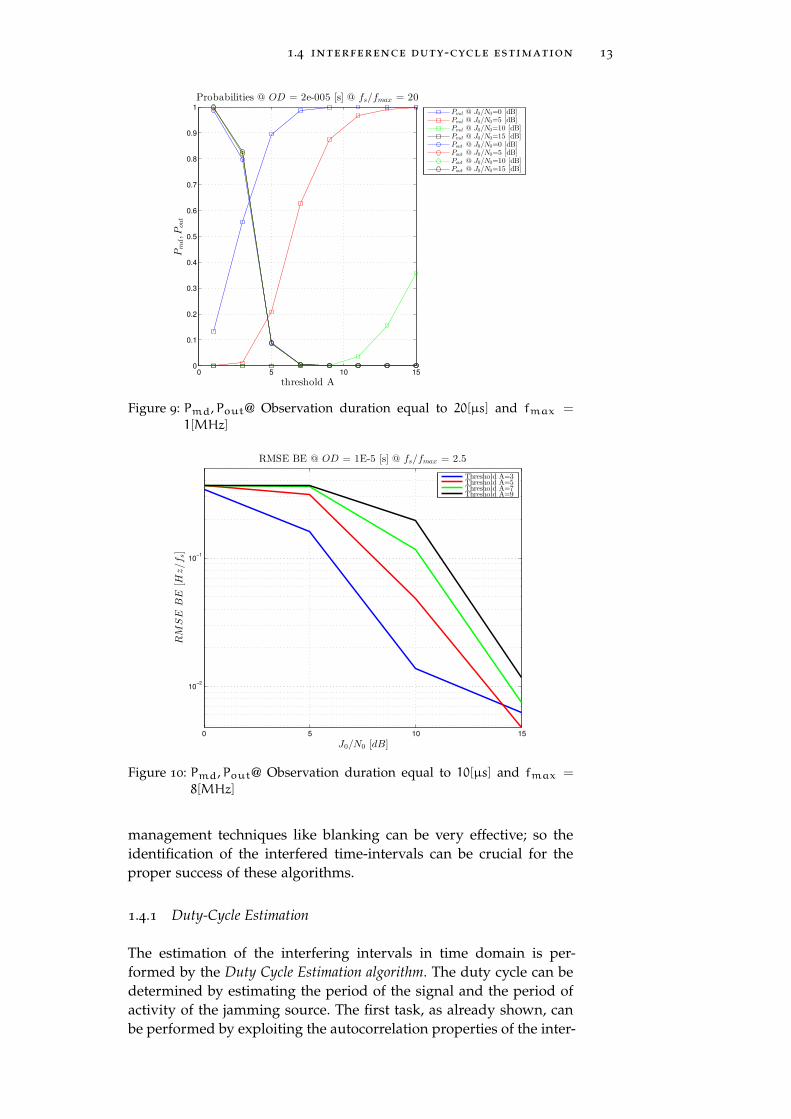
Figure 9 Pmd,Pout@ Observation duration equal to 20[µs]and fmax = 1[MHz] 13
Figure 10 Pmd,Pout@ Observation duration equal to 10[µs]and fmax = 8[MHz] 13
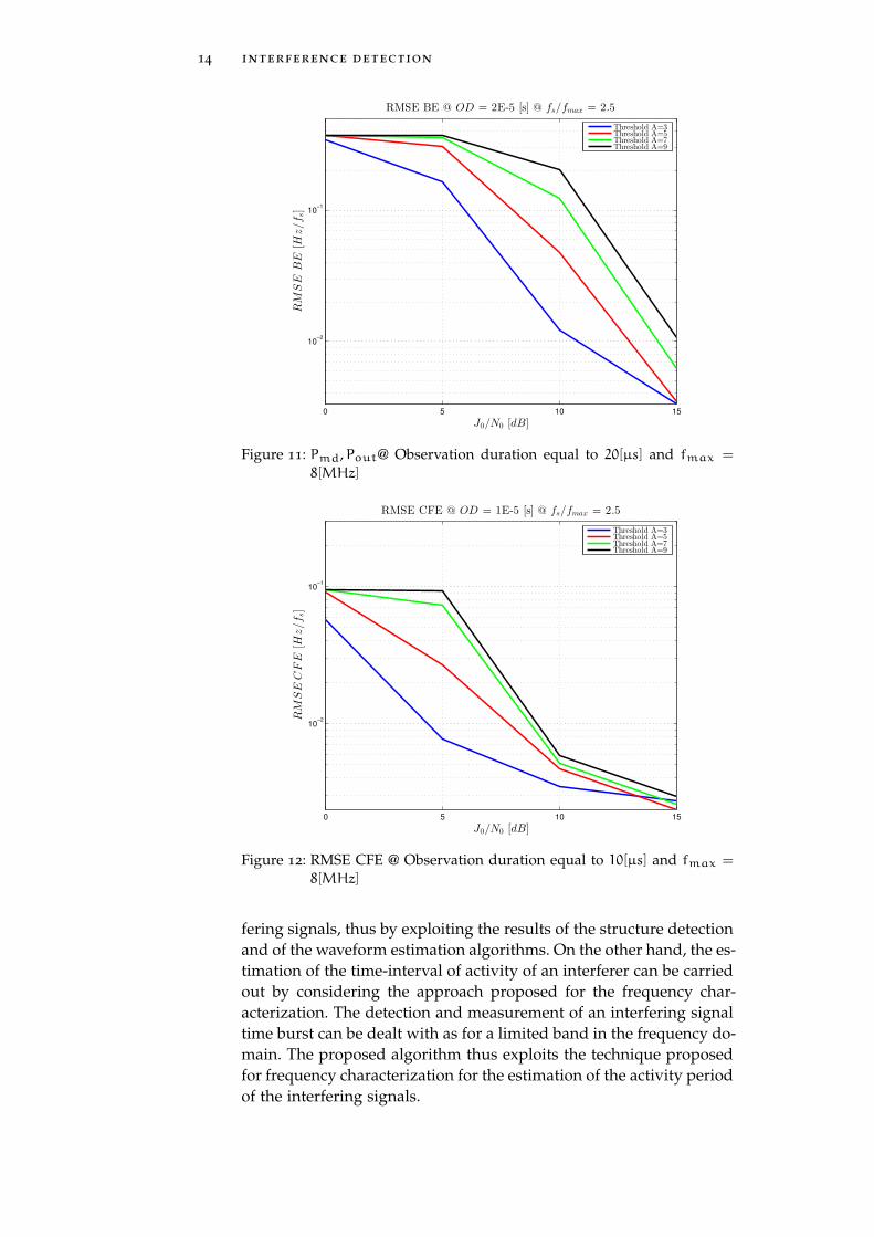
Figure 11 Pmd,Pout@ Observation duration equal to 20[µs]and fmax = 8[MHz] 14
Figure 12 RMSE CFE @ Observation duration equal to10[µs] and fmax = 8[MHz] 14
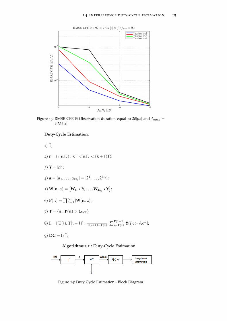
Figure 13 RMSE CFE @ Observation duration equal to20[µs] and fmax = 8[MHz] 15
Figure 14 Duty Cycle Estimation - Block Diagram 15
Figure 15 Pmd,Pout@ Duty Cycle equal to 0.05 18
Figure 16 Pmd,Pout@ Duty Cycle equal to 0.5 18
Figure 17 Pmd,Pout@ Duty Cycle equal to 0.8 19
Figure 18 RMSE DC @ Duty cycle equal to 0.05 19
Figure 19 RMSE DC @ Duty cycle equal to 0.5 20
Figure 20 RMSE DC @ Duty cycle equal to 0.5 20
Figure 21 RMSE CIE @ Duty cycle equal to 0.05 21
Figure 22 RMSE CIE @ Duty cycle equal to 0.5 21
Figure 23 RMSE CIE @ Duty cycle equal to 0.8 22
Figure 24 Spectrogram - Urban Chirp 25
Figure 25 Comparison PSD with LSP = 400 26
Figure 26 Spectrogram - Urban Tones 27
Figure 27 Comparison PSD with LSP = 400 27
Figure 28 Comparison PSD with LSP = 800 28
Figure 29 Spectrogram - Urban Chirp 28
Figure 30 Comparison PSD with LSP = 400 29
Figure 31 Spectrogram - Urban Chirp 29
Figure 32 Comparison PSD with LSP = 400 30
Figure 33 Spectrogram - Urban Wideband 30
xvii
xviii List of Figures
Figure 34 Comparison PSD with LSP = 400 31
Figure 35 Spectrogram - Urban Wideband 32
Figure 36 Comparison PSD with LSP = 400 32
Figure 37 Spectrogram - Urban Wideband 33
Figure 38 Comparison PSD with LSP = 400 33
Figure 39 Spectrogram - Urban Tones 34
Figure 40 Comparison PSD with LSP = 400 34
Figure 41 Comparison PSD with LSP = 800 35
Figure 42 Spectrogram - Urban Wideband 35
Figure 43 Comparison PSD with LSP = 400 36
Figure 44 Spectrogram - Urban Chirp 36
Figure 45 Comparison PSD with LSP = 400 37
Figure 46 Spectrogram - Urban Chirp 37
Figure 47 Comparison PSD with LSP = 400 38
Figure 48 Spectrogram - Urban Wideband 39
Figure 49 Comparison PSD with LSP = 400 39
Figure 50 Comparison PSD with LSP = 400 40
Figure 51 Comparison PSD with LSP = 400 40
Figure 52 Comparison PSD with LSP = 400 41
Figure 53 Detection Test withA = 4 and LSP = [200, 400, 800] 42
Figure 54 Spectrogram - Urban Chirp 42
Figure 55 Comparison PSD with LSP = 400 43
Figure 56 Comparison PSD with LSP = 400 43
Figure 57 Spectrogram - Urban Wideband 44
Figure 58 Comparison PSD with LSP = 400 44
Figure 59 Spectrogram - Urban Chirp 45
Figure 60 Comparison PSD with LSP = 400 45
Figure 61 Interferer Detection - Block Diagram. 50
Figure 62 Interferer Acquisition - Block Diagram. 55
Figure 63 Interferer Estimation - Flow graph. 57
Figure 64 Fresnel integral approximation. 62
Figure 65 (a)Approximation accuracy vs. interfering sig-nal bandwidth; (b) approximation accuracy vs.interfering signal period. 63
Figure 66 Probability of Detection - Classic Detector. 65
Figure 67 Probability of Detection - Optimize Detector. 65
Figure 68 MSE vs JNRR - Fs/fM = 10− T = 10[µs] − L =
10 67
Figure 69 MSE vs JNRR - Fs/fM = 10− T = 25[µs] − L =
10 68
Figure 70 MSE vs JNRR - Fs/fM = 10− T = 50[µs] − L =
10 68
Figure 71 Residual power after cancellation: T = 10µs,L = 10 71
Figure 72 Residual power after cancellation: T = 10µs,L = 100 71
Figure 73 Residual power after cancellation: T = 25µs,L = 10 72
Figure 74 Residual power after cancellation: T = 25µs,L = 100 72
List of Figures xix
Figure 75 Residual power after cancellation: T = 50µs,L = 10 73
Figure 76 Residual power after cancellation: T = 50µs,L = 100 73
Figure 77 Multipath Scenario 79
Figure 78 Estimated Autocorrelation function of Multi-path signal with 6 paths. 80
Figure 79 Zoom on Estimated Autocorrelation functionof Multipath signal with 6 paths. 80
Figure 80 Zoom on Estimated Autocorrelation functionof Multipath signal with 3 paths. 81
Figure 81 Zoom on Estimated Autocorrelation functionof Multipath signal with 3 paths. 81
Figure 82 Multipath - Probability of Detection. 83
Figure 83 Multipath - Probability of Detection. 83
Figure 84 Residual power after cancellation: T = 10µs,L = 10 84
Figure 85 Residual power after cancellation: T = 10µs,L = 100 85
Figure 86 Residual power after cancellation: T = 25µs,L = 10 85
Figure 87 Residual power after cancellation: T = 25µs,L = 100 86
Figure 88 Residual power after cancellation: T = 50µs,L = 10 86
Figure 89 Residual power after cancellation: T = 50µs,L = 100 87
Figure 90 Multipath Cancellation Residual - JNR = −10dB−
Fs/fM = 2− T = 10µs− L = 10 88
Figure 91 Multipath Cancellation Residual - JNR = 0dB−
Fs/fM = 2− T = 10µs− L = 10 88
Figure 92 Multipath Cancellation Residual - JNR = 10dB−
Fs/fM = 2− T = 10µs− L = 10 89
Figure 93 Multipath Cancellation Residual - JNR = 10dB−
Fs/fM = 2− T = 10µs− L = 100 89
Figure 94 Multipath Cancellation Residual - JNR = 10dB−
Fs/fM = 2− T = 10µs− L = 10 90
Figure 95 Multipath Cancellation Residual - JNR = 0dB−
Fs/fM = 10− T = 10µs− L = 10 90
Figure 96 Multipath Cancellation Residual - JNR = 0dB−
Fs/fM = 5− T = 10µs− L = 10 91
Figure 97 Multipath Cancellation Residual - JNR = 0dB−
Fs/fM = 2− T = 10µs− L = 10 91
Figure 98 Multipath Cancellation: Residual & GNSS - JNR =
−10dB− Fs/fM = 2− T = 10µs−L = 10 92
Figure 99 Multipath Cancellation: Residual & GNSS - JNR =
0dB− Fs/fM = 2− T = 10µs− L = 10 92
Figure 100 Multipath Cancellation: Residual & GNSS - JNR =
10dB− Fs/fM = 2− T = 10µs− L = 10 93
xx List of Figures
Figure 101 Multipath Cancellation: Residual & GNSS - JNR =
10dB− Fs/fM = 2− T = 10µs− L = 10 93
Figure 102 Multipath Cancellation: Residual & GNSS - JNR =
10dB− Fs/fM = 2− T = 10µs− L = 100 94
Figure 103 Multipath Cancellation: Residual & GNSS - JNR =
0dB− Fs/fM = 10− T = 10µs− L = 10 94
Figure 104 Multipath Cancellation: Residual & GNSS - JNR =
0dB− Fs/fM = 5− T = 10µs− L = 10 95
Figure 105 Multipath Cancellation: Residual & GNSS - JNR =
0dB− Fs/fM = 2− T = 10µs− L = 10 95
Figure 106 Typical GPS receiver with AGC shown 108
Figure 107 AGC gain for the baseline and three spoofedscenarios 112
Figure 108 Correlation profile for the baseline and threespoofed scenarios 113
Figure 109 Correlation metric 1 in baseline and three spoofedscenarios 114
Figure 110 Correlation metric 2 in baseline and three spoofedscenarios 114
Figure 111 Correlation metric 3 in baseline and three spoofedscenarios 114
Figure 112 Automatic Gain Control of a free RFI station115
Figure 113 Automatic Gain Control of a RFI station 115
Figure 114 AGC: comparison between FAI and ZMA-Astations 116
Figure 115 FAI station: AGC gain level and histogram 116
Figure 116 ZMA-A station: AGC gain level and histogram 117
Figure 117 FAI station: AGC gain level and C/N0 PRN14 117
Figure 118 ZMA-A station: AGC gain level and C/N0 PRN14 118
Figure 119 ZMA-A station: AGC gain level and C/N0 PRN18 119
Figure 120 ZMA-A station: AGC gain level and C/N0 PRN21 119
Figure 121 ZMA-A station: AGC gain level and C/N0 PRN22 120
Figure 122 ZMA-A station: AGC gain level and C/N0 PRN24 120
Figure 123 FAI station: C/N0 PRN 14 envelope 121
Figure 124 FAI station: Metric 1 residual for the PRN 14 121
Figure 125 FAI station: Zoom on C/N0 PRN 14 envelope 121
Figure 126 FAI station: Zoom Metric 1 residual for thePRN 14 122
Figure 127 ZMA-A station: Zoom C/N0 PRN 14 envelope 122
Figure 128 ZMA-A station: Zoom Metric 1 residual for thePRN 14 122
Figure 129 ZMA-A station: Zoom C/N0 PRN 18 envelope 122
Figure 130 ZMA-A station: Zoom Metric 1 residual for thePRN 18 123
Figure 131 ZMA-A station: Zoom C/N0 PRN 21 envelope 123
Figure 132 ZMA-A station: Zoom Metric 1 residual for thePRN 21 123
Figure 133 ZMA-A station: Zoom C/N0 PRN 22 envelope 123
Figure 134 ZMA-A station: Zoom Metric 1 residual for thePRN 22 124
Figure 135 ZMA-A station: Zoom C/N0 PRN 24 envelope 124
Figure 136 ZMA-A station: Zoom Metric 1 residual for thePRN 24 124
L I S T O F TA B L E S
Table 1 Simulation parameters for frequency charac-terization 8
Table 2 Algorithm parameters for frequency character-ization 9
Table 3 Simulation parameters for duty cycle estima-tion 17
Table 4 Algorithm parameters for frequency character-ization 17
Table 5 Update parameters for frequency characteriza-tion 25
Table 6 Detection - Simulation Parameter 64
Table 7 Estimation - Simulation Parameter 67
Table 8 Cancellation Parameter 70
Table 9 Simulation Parameters 79
Table 10 Detection - Simulation Parameter 82
Table 11 Cancellation - Simulation Parameter 87
Table 12 Spoofing Scenario Parameters 111
A C R O N Y M S
AWGN Additive White Gaussian Noise
AC Autocorrelation
AGC Automatic Gain Control
AOA Angle Of Arrival
xxi
xxii acronyms
BOC Binary Offset Carrier
CIE Central Instant Error
CN0 Carrier-to-Noise Ratio
CRB Cramer Rao Bound
DC Duty Cycle
DFT Discrete Fourier Transform
DLL Delay Lock Loop
DOA Direction of Arrival
DVB-T Digital Video Broadcast - Terrestrial
ESD Energy Spectral Density
FFT Fast Fourier Transform
FM Frequency Modulated
FT Fourier Transform
GNSS Global Navigation Satellite System
GPS Global Positioning System
ICC Interference Characterization and Cancellation
IFFT Inverse FFT
IIR Infinite Impulse Response
JNR Jammer-to-Noise Ratio
LNA Low Noise Amplifier
LOS Line of Sight
ML Maximum Likelihood
MSE Mean Square Error
OD Obsevation Duration
PLL Phase-Locked Loop
PM Phase Modulated
PPD Personal Privacy Device
PRN Pseudorandom Noise
PSD Power Spectral Density
PVT Position-Velocity-Time
RAIM Receive Autonomous Integrity Monitoring

acronyms xxiii
RFI Radio Frequency Interference
RMS Root Mean Square
RMSE Root Mean Square Error
SQM Signal Quality Monitoring
TDOA Time Difference Of Arrival
WT Wavelet Transform

Part I
I N T E R F E R E N C E M A N A G E M E N T T E C H N I Q U E S
Due to their low power levels, GNSS signals are highly sus-ceptible to both intentional and unintentional RFI sourcesdisruptions. The increasing diversification of everyday lifeapplications based on satellite navigation systems requiresa high reliability of the communication link, in each stepfrom the transmission to the reception one, above all forthe safety-critical applications [45]. Jamming signals, whichcan deteriorate or even deny the provided GNSS services,and unintentional RFI sources, as malfunctioning elements,represent a paramount problem in GNSS operating chain.Thus, the problem of how to face RFI, and in particularthe intentional one, has become a hot topic in recent years[12], [P4],[9]. For this reason, it is necessary to define solu-tions able to guarantee and to maintain the GNSS serviceand reliability in presence of such threats.
The aim of this thesis is to analyze the problem and topropose new solutions able to counteract interfering sig-nals. In particular, the main aim is to design techniques inorder to detect the presence of interfering signals, to local-ize the malicious sources, and to mitigate and reduce theireffects.

1I N T E R F E R E N C E D E T E C T I O N
1.1 introduction
The diversity of the GNSS [58] based applications in the majority ofthe human life habits increases its importance and consequently itsvulnerability against malicious attacks. As well known, the GNSS sig-nals hare broadcast and received at a very low power level at thereceiver side and for this reason are very vulnerable to the RFI effects,both unintentionally and intentionally generated [45]. The maliciousattacks aim to degrade the performance of all that systems and appli-cations based on correct information of timing and positioning pro-vided by the GNSS, leading to the complete disruption of the service[8][7][61][13][33]. The higher the jamming power, the more danger-ous the consequence on the GNSS quality of service. Due to thesepowerful issues, it is necessary to design techniques able to contrastinterfering effects and to minimize their disruptive aims. The firststep is to identify if an interferer is present or not. In literature, sev-eral detection techniques have been proposed based on the analysisof signal outputs of blocks in the reception chain as Automatic GainControl (AGC) [32], Carrier-to-Noise Ratio (CN0) evaluation [39] andcooperative techniques which exploit correlator metric informationfrom distributed nodes [70]. The major part of detection techniquesis essentially based on the Time Difference Of Arrival (TDOA) and An-gle Of Arrival (AOA) estimation methods and some research worksanalyzed also the Direction of Arrival (DOA) estimates [71]; some re-searchers also studied a possible combination of the cited techniques[18].Instead, in this work a different interference detection approach ispresented. The method is performed in the frequencies domain, thusexploiting spectral signatures of the jamming signals, moving fromthe above cited and widely used localization techniques. Our tech-nique exploits the Wavelet Transform (WT) of the Power Spectral Den-sity (PSD) of the interfering signal. By means of the time-scale trans-form, it is possible to detect discontinuities in the received signal spec-trum, corresponding to the higher values of the wavelet coefficients.Once transients are detected it is possible to estimate the bandwidthof the jamming signal and to evaluate the mean spectral energy. Fur-thermore, this method is also applied in the time-domain in order todefine the time envelope of the received signal. The goal is to deter-mine the duty cycle of the signal, and so the periodical repetition ofthe interfering event. The algorithms have been thoroughly described,and validated by means of numerical simulations and results withboth synthetized signal by MATLAB tool and collected data in con-trolled scenarios [Pr1].The rest of the chapter is structured as follows: in Section 1.2 the sys-
3
4 interference detection
tem model is present; in Section 1.3 and Section 1.4 the approachesin the frequency domain and time domain are described, and vali-dated by performance evaluation and numerical results, respectively;in Section 1.5 an update version of the frequency domain approach isdescribed with several numerical results obtained by testing our algo-rithm with data, collected in controlled scenario. Concluding remarksare given in Section 1.6
1.2 system model
Previously an introduction to the most common approaches for inter-ference detection in GNSS has been provided. As already explained,the interfering signals aim to deteriorate the communication betweentransmitter and receiver. The malicious signal is received with theuseful signal trying to corrupt the receiver’s capabilities in decodingcorrect information and PVT solutions. The received signal at the tar-get device can be expressed as [28][65]:
r(t) =
Ns∑k=1
√Pksk (t− τk) e
j(θk+2πfkt) (1)
+√PIsI (t− τI) e
j(θI+2πfIt) +w(t)
where Ns is the number of satellite signals, Pk and PI are the usefulsignal power of the k-th satellite and the interference power, respec-tively; τk, fk, θk and τI, fI, θI are the time delay, frequency and phaseoffset of the useful signal and the interfering signal respectively, w(t)is the Additive White Gaussian Noise (AWGN) with power spectraldensity equal to σ2w. Considering bicA = b iAc and |i|A = i mod A, thek-th satellite signal can be expressed as [28]:
sk(t) =
+∞∑l=−∞Dk (blcLs)ak (blcLs)g (t− lTc) (2)
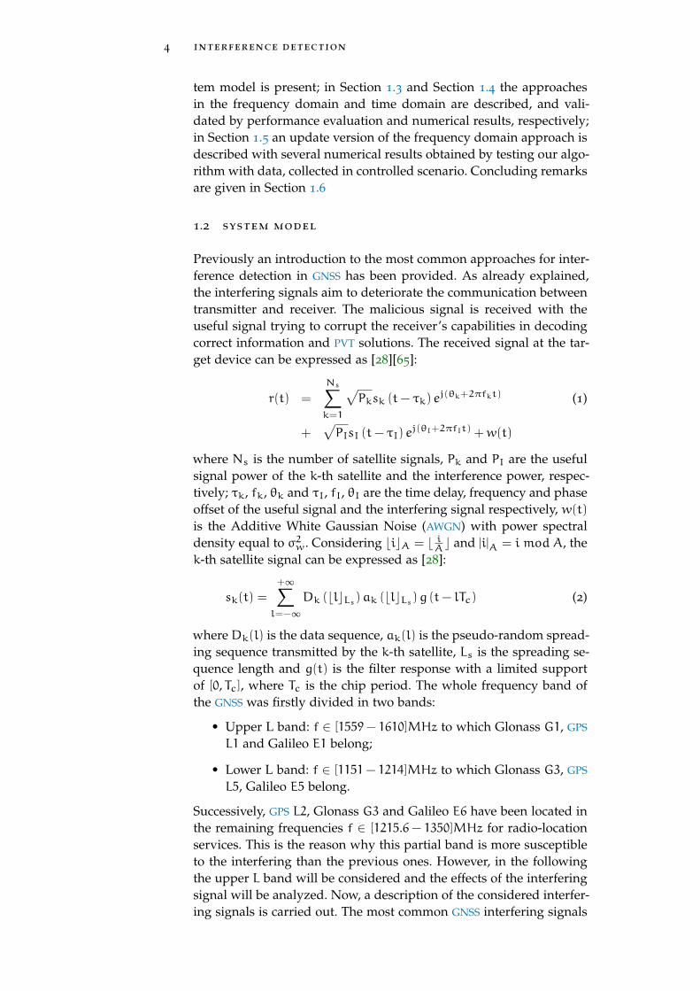
whereDk(l) is the data sequence, ak(l) is the pseudo-random spread-ing sequence transmitted by the k-th satellite, Ls is the spreading se-quence length and g(t) is the filter response with a limited supportof [0, Tc], where Tc is the chip period. The whole frequency band ofthe GNSS was firstly divided in two bands:
• Upper L band: f ∈ [1559− 1610]MHz to which Glonass G1, GPS
L1 and Galileo E1 belong;
• Lower L band: f ∈ [1151− 1214]MHz to which Glonass G3, GPS
L5, Galileo E5 belong.
Successively, GPS L2, Glonass G3 and Galileo E6 have been located inthe remaining frequencies f ∈ [1215.6− 1350]MHz for radio-locationservices. This is the reason why this partial band is more susceptibleto the interfering than the previous ones. However, in the followingthe upper L band will be considered and the effects of the interferingsignal will be analyzed. Now, a description of the considered interfer-ing signals is carried out. The most common GNSS interfering signals
1.3 interference band detection 5
are defined by periodic envelope, with particular Autocorrelation (AC)function characteristics [12],[48]. Current interfering waveforms aredefined by angle modulated signals which have a periodic core z(t).They can be written as:
sFM
(t) = A exp{j2π
(f0t+
∫t−∞ z(ξ)dξ
)}(3)
sPM
(t) = A exp {j2π (f0t+ z(t))} (4)
which correspond to Frequency Modulated (FM) and Phase Modu-lated (PM), respectively. For a generic and periodic modulation func-tion
z(t) =∑k
z0(t− kT) (5)
and consequently the equations (3) and (4) can be rewritten, respec-tively, as:
sFM
(t) =∑k
AksFM(t− kT)eΘFM(k) (6)
sPM
(t) =∑k
AksPM(t− kT)eΘPM(k) (7)
These signals are defined as structured signals due to their peri-odic core waveform. Due to these properties, they can be classifiedas parametric waveforms because by exploiting AC characteristics itis possible to represents them by means of specific parameters, esti-mated by tracking the periodic waveform. However, it is worthwhileto notice that among interfering signals also non parametric wave-forms are presents. These kind of signals do not present periodic en-velope and consequently particular AC characteristics and thus theycannot be identified by a parametric representation. Non-parametricwaveforms represent a more difficult family of interfering signals thatare more difficult to characterize and classify simply because a prioriinformation is not available. Accordingly, solutions to detect and es-timate this kind of signals are the spectrum estimation techniquesand time-scale and time-frequency mathematical tool, able to extractprimary information from the received signal [53].
1.3 interference band detection
As mentioned previously, several interference detection techniqueshave been proposed and deeply discussed in literature. By exploit-ing the well known WT [21], it is possible to estimate the interferencebandwidth, for both structured and non-structured interference. In
6 interference detection
the last case, bandwidth estimation is one of the few information re-garding the received interfering signal. In [25] and [54] interferencemitigation algorithms that exploit WT are presented. This mathemati-cal tool allows for identification and reconstruction of the interferingsignal due to the split in the time-scale domain from the useful sig-nal, with interesting results in terms of mitigation purposes. The basicidea is to use the wavelet coefficients, the output of the WT on the PSD
of the signal, as the identifiers of the transient processes in the PSD
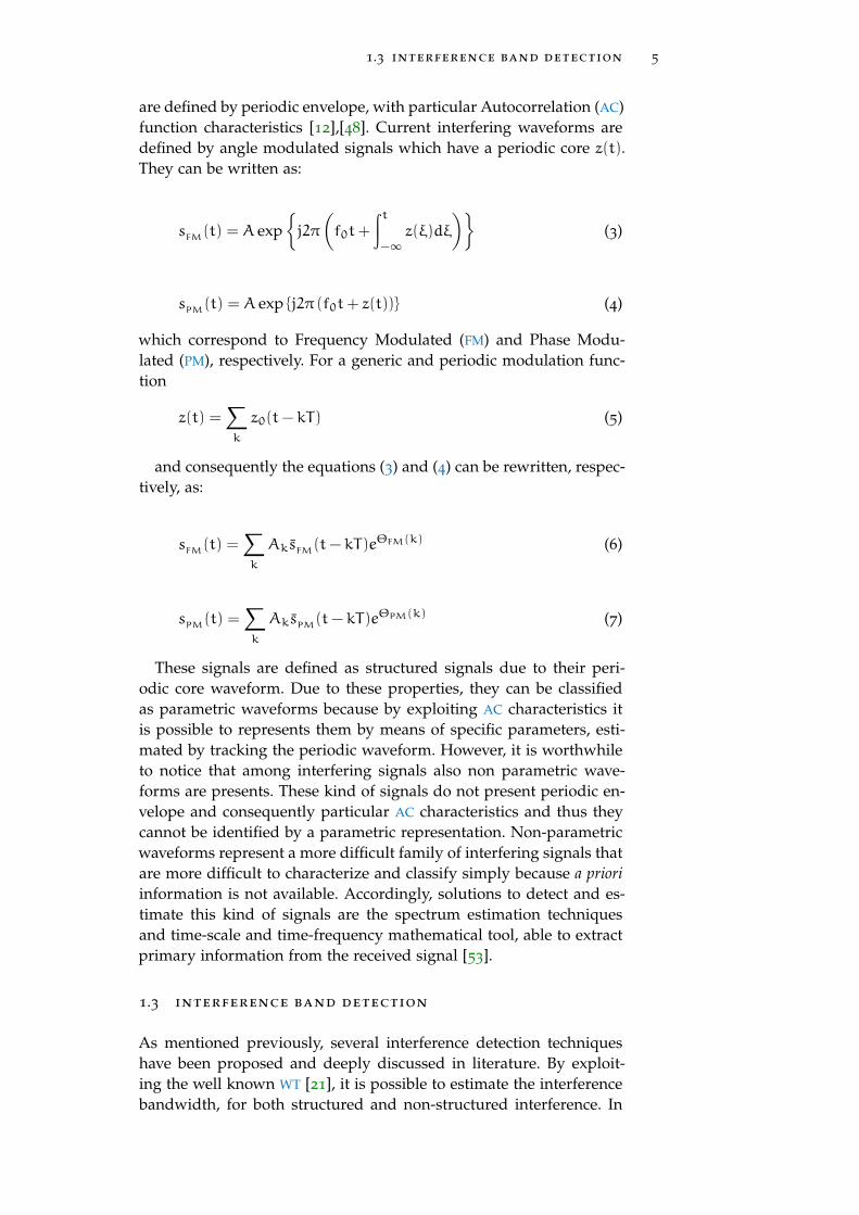
envelope. In particular, the discontinuities of the signal correspond tohigh values of the wavelet coefficients. Once the discontinuities havebeen detected, the PSD samples to which a high coefficient value corre-spond are identified, and it is thus possible to localize the signal in thefrequency domain, and to evaluate the mean interference energy. Thecharacterization algorithm identifies the bands inside which most ofthe interfering signal energy is concentrated. More in particular, thisalgorithm provide means to determine how the interfering signal isdistributed in the frequency domain, and consequently it is possibleto determine the number and the dimension of the interfered band-widths. The Band Detection algorithm exploits the WT of the receivedsignal PSD in order to detect interfered bands. By means of the WT, itis possible to identify where any discontinuities is localized. The pro-posed algorithm is described by the pseudo code in the algorithm1
and shown in the block diagram in Figure (1).
Frequency Characterization & Band Detection;;1) r = {r(nTs) : kOD < nTs < (k+ 1)OD};;2) S = |fft(r)|2;;3) a = [a1, . . . ,aNs ] = [21, . . . , 2Ns ];;4) W(n,a) =
[Wa1 ? S, . . . , WaNs
? §];
;5) P(n) =
∏Nsa=1 |W(n,a)|;
;6) F = {n : P(n) > ξWT };;
7) B = {[F(i), F(i+ 1)] :; 1F(i+1)−F(i) ;
∑F(i+1)j=F(i) S(j);> Aσ2};
;Algorithmus 1 : Frequency Characterization & Band Detection
Figure 1: Band Detection - Block Diagram
1.3 interference band detection 7
The procedure consists in sampling the received signal in a timewindow of Obsevation Duration (OD)(line 1) and then the PSD is cal-culated (line 2). In order to perform WT it is necessary to select thescale factors, according to the resolution to be achieved. The scale fac-tors have been chosen to be the set of powers of 2, ranging from 2
to 2Ns (line 3). The time-scale transform is then evaluated for eachscale factor, which identifies different frequency bands with differentresolutions. The chosen mother wavelet is the Haar wavelet functionφ(t) defined as:
φ(t) =
1 0 < t < 1/2
−1 −1/2 < t < 0
0 otherwise
For each scale factor the WT can be implemented as the convolutionbetween the wavelet function and the signal S (line 4). The output ofthe convolution is a matrix with each row corresponding to a scalefactor and each column corresponding to a time instant. If a disconti-nuity is present in the PSD envelope, the wavelet coefficient, obtainedfrom the convolution, is very high. Through this analysis it is pos-sible to identify the discontinuities of the signal, in particular whenand also where, at which sample, the signal shows transients. Subse-quently, for each time instant, the product of the absolute values ofthe wavelet transform corresponding to the different scale factors iscalculated, as indicated in line (5). The rationale is that if a PSD dis-continuity exists for a certain frequency value, this results in a highwavelet transform, for all the scale factors; taking the product of theabsolute values helps eliminating undesired peaks due to noise. Fre-quencies corresponding to peaks of the sequence obtained as resultof the previous product are selected. In order to eliminate undesiredmeasurements due to noise a comparison with a threshold is per-formed, as indicated at line (6). The power of each detected interfererband, comprised between two successive detected frequencies, is com-pared to a threshold, and only those bands in which the mean powerspectral density crosses the threshold are identified (line 7).
1.3.1 Performance Analysis
The performance evaluation for the above algorithm is presented be-low.
1.3.1.1 Performance Evaluation Criteria
The chosen performance evaluation criteria are the Probability of MissedDetection (Pmd) and the Probability of Outlier (Pout). We define Pmd asthe probability of not-detecting the presence of the interfering signalwithin the interfered band. On the other hand, we identify Pout as theprobability of detecting at least an interfered band event outside theideal interferer interval. These kinds of detected events are classified
8 interference detection
J0/N0 [0, 5, 10, 15] [dB]
Minimum frequency 0.5 [MHz]
Maximum Frequency [8, 4, 2, 1]
Table 1: Simulation parameters for frequency characterization
as outliers because they are detected outside the real interferer signaland so they are the results of a wrong detection analysis. Under thehypothesis of correct detection, we also evaluate the accuracy of thebandwidth measurements. In particular, we evaluate the mean errorof estimation of the central frequency fc defined as
ec =√E[|fc − fc|2
](8)
defined as the difference between the estimated central frequency ofthe interfered band and the estimated central frequency, and the errorof the estimated bandwidth
ec =√E[|B−B|2
](9)
defined as the difference between the estimated bandwidth and theinterfered bandwidth. Previous errors have been estimated by meansof Root Mean Square Error (RMSE) for both the central frequency error(RMSE CFE) and the bandwidth error (RMSE BE).
1.3.1.2 Scenario
Simulation tests are carried out considering an interfering signal em-bedded in Additive White Gaussian Noise (AWGN) with a power spec-tral density ratio J0/N0 ranging from 0 to 15 dB. We consider wideband interfering signal with power lower than the saturation level.The minimum frequency is set equal to 500kHz and the maximumfrequency is determined from the fs/fmax factor, which interval isset equal to [2.5, 5, 10, 15].
1.3.1.3 Algorithm Optimization
In the following the parameters characterizing the algorithm are pre-sented. The parameters are resumed in table 2. An observation du-ration OD equal to 10, 20[µs] has been considered in order to followalso rapid variations of the signal frequency characteristics. The num-ber of scales factors considered has been calculated according to thedimension of the observable length. In particular maximum waveletduration equal to one fourth of the observable duration has been con-sidered. A wavelet threshold equal to twice the variance of noise afterthe wavelet transform has been considered. This is due to the fact that,according to the Central Limit Theorem, the distribution of the Haarwavelet transform of the square of a noise sequence with i.i.d. sam-ples distributed as Gaussian random variables with zero mean andvariance σ2 (∼ N(0,σ2)), converges to a Gaussian random variablewith zero mean variance equal to 2σ2 (∼ N(0, 2σ2)). Different valuesfor the last verification threshold are selected as shown in table 2
1.3 interference band detection 9
Sampling Frequency fs 20 [MHz]
Observation Duration OD 10, 20[µs]
Number of scales factors Ns round((log2(OD))-2)
Wavelet threshold ξWT 2(2σ2)Ns
Mean PSD threshold Aσ2 A=[1, 3, 5, 7, 9, 11, 15]
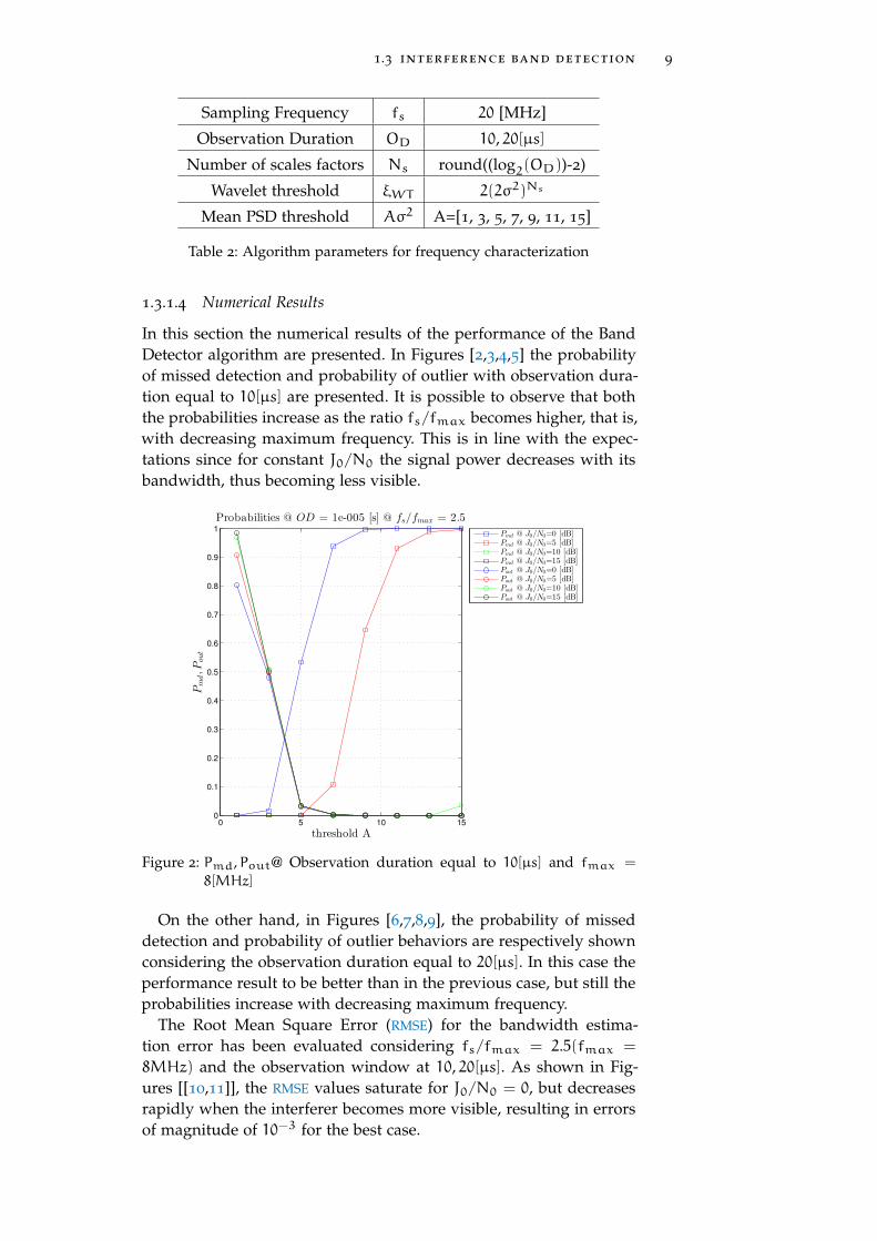
Table 2: Algorithm parameters for frequency characterization
1.3.1.4 Numerical Results
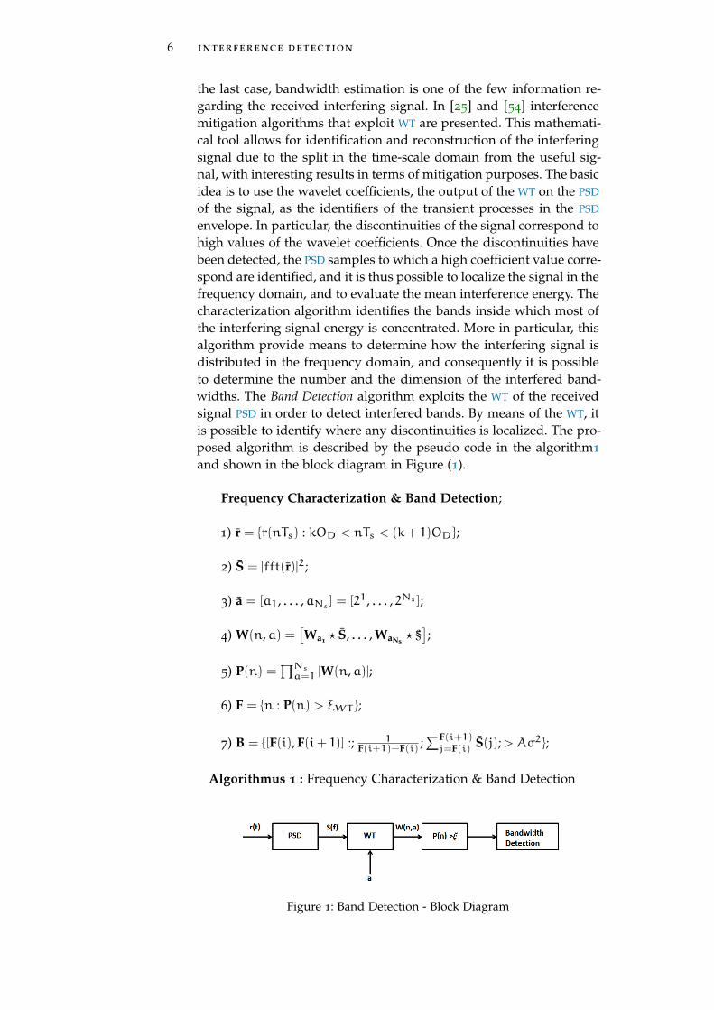
In this section the numerical results of the performance of the BandDetector algorithm are presented. In Figures [2,3,4,5] the probabilityof missed detection and probability of outlier with observation dura-tion equal to 10[µs] are presented. It is possible to observe that boththe probabilities increase as the ratio fs/fmax becomes higher, that is,with decreasing maximum frequency. This is in line with the expec-tations since for constant J0/N0 the signal power decreases with itsbandwidth, thus becoming less visible.
0 5 10 150
0.1
0.2
0.3
0.4
0.5
0.6
0.7
0.8
0.9
1
threshold A
Pmd,P
out
Probabilities @ OD = 1e-005 [s] @ fs/fmax = 2.5
Pmd @ J0/N0=0 [dB]Pmd @ J0/N0=5 [dB]Pmd @ J0/N0=10 [dB]Pmd @ J0/N0=15 [dB]Pout @ J0/N0=0 [dB]Pout @ J0/N0=5 [dB]Pout @ J0/N0=10 [dB]Pout @ J0/N0=15 [dB]
Figure 2: Pmd,Pout@ Observation duration equal to 10[µs] and fmax =
8[MHz]
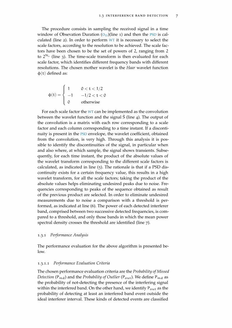
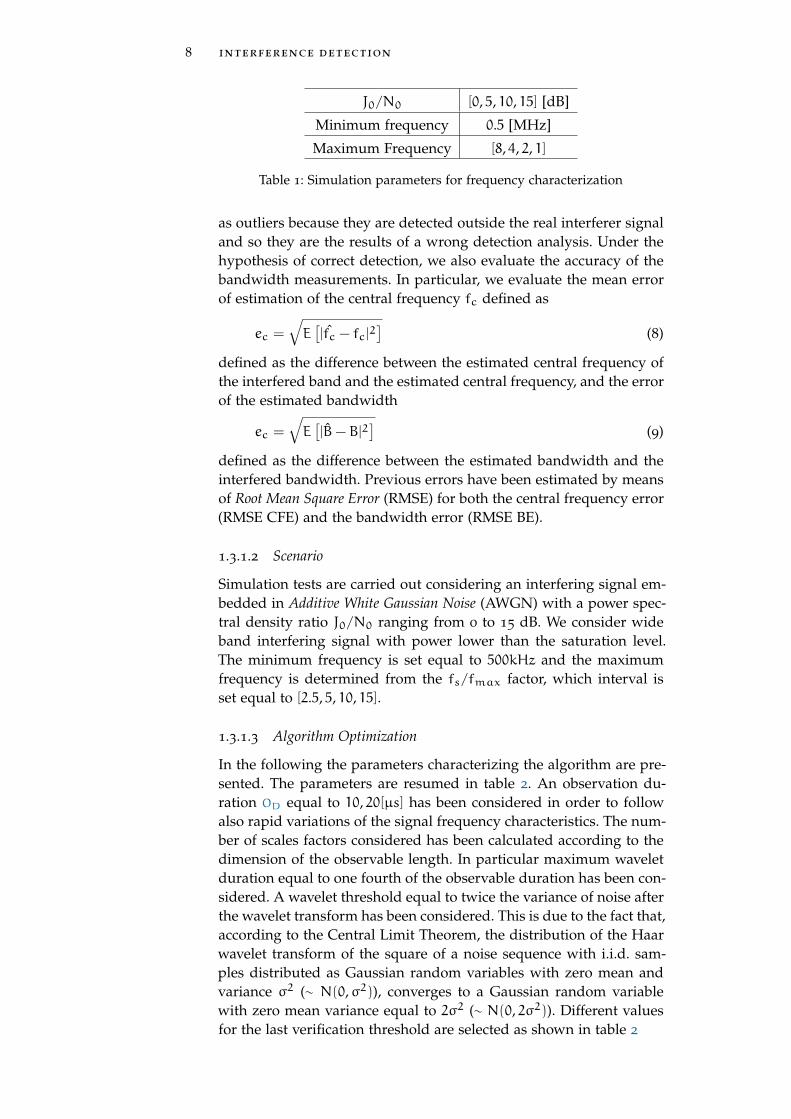
On the other hand, in Figures [6,7,8,9], the probability of misseddetection and probability of outlier behaviors are respectively shownconsidering the observation duration equal to 20[µs]. In this case theperformance result to be better than in the previous case, but still theprobabilities increase with decreasing maximum frequency.
The Root Mean Square Error (RMSE) for the bandwidth estima-tion error has been evaluated considering fs/fmax = 2.5(fmax =
8MHz) and the observation window at 10, 20[µs]. As shown in Fig-ures [[10,11]], the RMSE values saturate for J0/N0 = 0, but decreasesrapidly when the interferer becomes more visible, resulting in errorsof magnitude of 10−3 for the best case.
10 interference detection
0 5 10 150
0.1
0.2
0.3
0.4
0.5
0.6
0.7
0.8
0.9
1
threshold A
Pmd,P
out
Probabilities @ OD = 1e-005 [s] @ fs/fmax = 5
Pmd @ J0/N0=0 [dB]Pmd @ J0/N0=5 [dB]Pmd @ J0/N0=10 [dB]Pmd @ J0/N0=15 [dB]Pout @ J0/N0=0 [dB]Pout @ J0/N0=5 [dB]Pout @ J0/N0=10 [dB]Pout @ J0/N0=15 [dB]
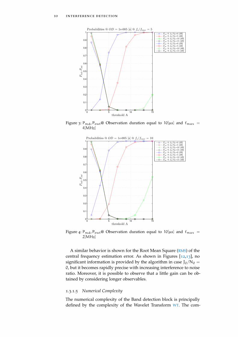
Figure 3: Pmd,Pout@ Observation duration equal to 10[µs] and fmax =
4[MHz]
0 5 10 150
0.1
0.2
0.3
0.4
0.5
0.6
0.7
0.8
0.9
1
threshold A
Pmd,P
out
Probabilities @ OD = 1e-005 [s] @ fs/fmax = 10
Pmd @ J0/N0=0 [dB]Pmd @ J0/N0=5 [dB]Pmd @ J0/N0=10 [dB]Pmd @ J0/N0=15 [dB]Pout @ J0/N0=0 [dB]Pout @ J0/N0=5 [dB]Pout @ J0/N0=10 [dB]Pout @ J0/N0=15 [dB]
Figure 4: Pmd,Pout@ Observation duration equal to 10[µs] and fmax =
2[MHz]
A similar behavior is shown for the Root Mean Square (RMS) of thecentral frequency estimation error. As shown in Figures [12,13], nosignificant information is provided by the algorithm in case J0/N0 =0, but it becomes rapidly precise with increasing interference to noiseratio. Moreover, it is possible to observe that a little gain can be ob-tained by considering longer observables.
1.3.1.5 Numerical Complexity
The numerical complexity of the Band detection block is principallydefined by the complexity of the Wavelet Transform WT. The com-
1.3 interference band detection 11
0 5 10 150
0.1
0.2
0.3
0.4
0.5
0.6
0.7
0.8
0.9
1
threshold A
Pmd,P
out
Probabilities @ OD = 1e-005 [s] @ fs/fmax = 20
Pmd @ J0/N0=0 [dB]Pmd @ J0/N0=5 [dB]Pmd @ J0/N0=10 [dB]Pmd @ J0/N0=15 [dB]Pout @ J0/N0=0 [dB]Pout @ J0/N0=5 [dB]Pout @ J0/N0=10 [dB]Pout @ J0/N0=15 [dB]
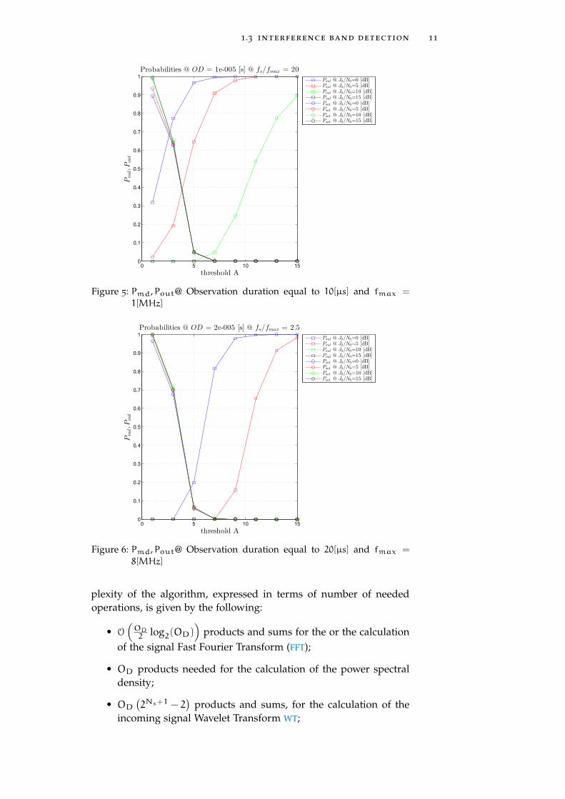
Figure 5: Pmd,Pout@ Observation duration equal to 10[µs] and fmax =
1[MHz]
0 5 10 150
0.1
0.2
0.3
0.4
0.5
0.6
0.7
0.8
0.9
1
threshold A
Pmd,P
out
Probabilities @ OD = 2e-005 [s] @ fs/fmax = 2.5
Pmd @ J0/N0=0 [dB]Pmd @ J0/N0=5 [dB]Pmd @ J0/N0=10 [dB]Pmd @ J0/N0=15 [dB]Pout @ J0/N0=0 [dB]Pout @ J0/N0=5 [dB]Pout @ J0/N0=10 [dB]Pout @ J0/N0=15 [dB]
Figure 6: Pmd,Pout@ Observation duration equal to 20[µs] and fmax =
8[MHz]
plexity of the algorithm, expressed in terms of number of neededoperations, is given by the following:
• O(OD2 log2(OD)
)products and sums for the or the calculation
of the signal Fast Fourier Transform (FFT);
• OD products needed for the calculation of the power spectraldensity;
• OD(2Ns+1 − 2
)products and sums, for the calculation of the
incoming signal Wavelet Transform WT;
12 interference detection
0 5 10 150
0.1
0.2
0.3
0.4
0.5
0.6
0.7
0.8
0.9
1
threshold A
Pmd,P
out
Probabilities @ OD = 2e-005 [s] @ fs/fmax = 5
Pmd @ J0/N0=0 [dB]Pmd @ J0/N0=5 [dB]Pmd @ J0/N0=10 [dB]Pmd @ J0/N0=15 [dB]Pout @ J0/N0=0 [dB]Pout @ J0/N0=5 [dB]Pout @ J0/N0=10 [dB]Pout @ J0/N0=15 [dB]
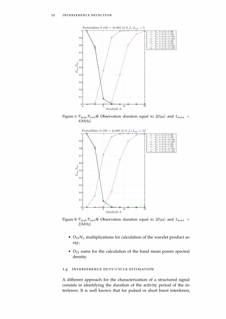
Figure 7: Pmd,Pout@ Observation duration equal to 20[µs] and fmax =
4[MHz]
0 5 10 150
0.1
0.2
0.3
0.4
0.5
0.6
0.7
0.8
0.9
1
threshold A
Pmd,P
out
Probabilities @ OD = 2e-005 [s] @ fs/fmax = 10
Pmd @ J0/N0=0 [dB]Pmd @ J0/N0=5 [dB]Pmd @ J0/N0=10 [dB]Pmd @ J0/N0=15 [dB]Pout @ J0/N0=0 [dB]Pout @ J0/N0=5 [dB]Pout @ J0/N0=10 [dB]Pout @ J0/N0=15 [dB]
Figure 8: Pmd,Pout@ Observation duration equal to 20[µs] and fmax =
2[MHz]
• ODNs multiplications for calculation of the wavelet product ar-ray;
• OD sums for the calculation of the band mean power spectraldensity.
1.4 interference duty-cycle estimation
A different approach for the characterization of a structured signalconsists in identifying the duration of the activity period of the in-terferers. It is well known that for pulsed or short burst interferers,
1.4 interference duty-cycle estimation 13
0 5 10 150
0.1
0.2
0.3
0.4
0.5
0.6
0.7
0.8
0.9
1
threshold A
Pmd,P
out
Probabilities @ OD = 2e-005 [s] @ fs/fmax = 20
Pmd @ J0/N0=0 [dB]Pmd @ J0/N0=5 [dB]Pmd @ J0/N0=10 [dB]Pmd @ J0/N0=15 [dB]Pout @ J0/N0=0 [dB]Pout @ J0/N0=5 [dB]Pout @ J0/N0=10 [dB]Pout @ J0/N0=15 [dB]
Figure 9: Pmd,Pout@ Observation duration equal to 20[µs] and fmax =
1[MHz]
0 5 10 15
10−2
10−1
J0/N0 [dB]
RM
SE
BE
[Hz/f s]
RMSE BE @ OD = 1E-5 [s] @ fs/fmax = 2.5
Threshold A=3Threshold A=5Threshold A=7Threshold A=9
Figure 10: Pmd,Pout@ Observation duration equal to 10[µs] and fmax =
8[MHz]
management techniques like blanking can be very effective; so theidentification of the interfered time-intervals can be crucial for theproper success of these algorithms.
1.4.1 Duty-Cycle Estimation
The estimation of the interfering intervals in time domain is per-formed by the Duty Cycle Estimation algorithm. The duty cycle can bedetermined by estimating the period of the signal and the period ofactivity of the jamming source. The first task, as already shown, canbe performed by exploiting the autocorrelation properties of the inter-
14 interference detection
0 5 10 15
10−2
10−1
J0/N0 [dB]
RM
SE
BE
[Hz/f s]
RMSE BE @ OD = 2E-5 [s] @ fs/fmax = 2.5
Threshold A=3Threshold A=5Threshold A=7Threshold A=9
Figure 11: Pmd,Pout@ Observation duration equal to 20[µs] and fmax =
8[MHz]
0 5 10 15
10−2
10−1
J0/N0 [dB]
RM
SECFE
[Hz/f s]
RMSE CFE @ OD = 1E-5 [s] @ fs/fmax = 2.5
Threshold A=3Threshold A=5Threshold A=7Threshold A=9
Figure 12: RMSE CFE @ Observation duration equal to 10[µs] and fmax =
8[MHz]
fering signals, thus by exploiting the results of the structure detectionand of the waveform estimation algorithms. On the other hand, the es-timation of the time-interval of activity of an interferer can be carriedout by considering the approach proposed for the frequency char-acterization. The detection and measurement of an interfering signaltime burst can be dealt with as for a limited band in the frequency do-main. The proposed algorithm thus exploits the technique proposedfor frequency characterization for the estimation of the activity periodof the interfering signals.
1.4 interference duty-cycle estimation 15
0 5 10 15
10−2
10−1
J0/N0 [dB]
RM
SECFE
[Hz/f s]
RMSE CFE @ OD = 2E-5 [s] @ fs/fmax = 2.5
Threshold A=3Threshold A=5Threshold A=7Threshold A=9
Figure 13: RMSE CFE @ Observation duration equal to 20[µs] and fmax =
8[MHz]
Duty-Cycle Estimation;;1) T ;;2) r = {r(nTs) : kT < nTs < (k+ 1)T };;3) Y = |r|2;;4) a = [a1, . . . ,aNs ] = [21, . . . , 2Ns ];;5) W(n,a) =
[Wa1 ? Y, . . . , WaNs
? Y];
;6) P(n) =
∏Nsa=1 |W(n,a)|;
;7) T = {n : P(n) > ξWT };;
8) I = {[T(i), T(i+ 1)] : 1T(i+1)−T(i) ;
∑T(i+1)j=T(i) Y(j);> Aσ2};
;9) DC = I/T ;;
Algorithmus 2 : Duty-Cycle Estimation
Figure 14: Duty Cycle Estimation - Block Diagram
16 interference detection
As the Band Detection algorithm, the Duty Cycle Estimation can bedescribed according to the pseudo-code in Algorithm 2 and shown inblock diagram in Figure (14). Firstly, the period estimate from the AC
analysis is considered (line 1) in order to define each signal periodrepetition. In line 3 the energy of the signal is computed. In order toperform WT it is necessary to select the scale factor, according to theresolution to be achieved. The scale factors have been chosen to bethe set of powers of 2, ranging from 2 to 2Ns (line 4). The time-scaletransform is then evaluated for each scale factor (line 5) and the prod-uct of all the WT outputs is performed (line 6). In order to eliminateundesired measurements due to noise a comparison with a thresh-old is performed, as indicated in line 7. The power of each interferinginterval is calculated and successively compared with a threshold pro-portional to the noise power. Finally, the duty-cycle of the interferingsignal is estimated as the ratio between the detected intervals and theperiod estimate. The main difference with respect to the previouslypresented results consists in the evaluation of the power envelope ofthe signal, as indicated at line (3) since, in this case, the time char-acteristics must be obtained. The algorithm provides information onboth the burst localization and on the duty-cycle values.
1.4.2 Performance Analysis
1.4.2.1 Performance Evaluation Criteria
As for the previous case performance has been evaluated in termsof probability of detection Pmd and in terms of probability of outlierPout. Moreover, in order to evaluate the accuracy of the proposedsolution, the mean error
ec =√E(|tc − tc|2
)(10)
defined as the difference between the estimated central instant of theinterfering burst signal and the real instant, and the mean error
eD =√E(|I− I|2
)(11)
defined as the difference between the duration estimation and thereal burst duration, have been estimated.
1.4.2.2 Scenario
As for the previous case, simulation tests are carried out consideringan interfering signal embedded in AWGN with an interfering signalpower to noise ratio J/N ranging from 0 to 15 [dB]. We consider sig-nals with a period equal to 10 and 20[µs]. The generated signals arechirp signals with instantaneous frequencies rapidly growing overthe receiver bandwidth, thus generating duty cycle values equal to0.05, 0.5 and 0.8. Parameters are shown in table 3.
1.4 interference duty-cycle estimation 17
Interference-to-Noise-Ratio J/N [0, 5, 10, 15] [dB]
Signal Period T 10, 20[µs]
Duty Cycle DC [0.05, 0.5, 0.8]
Table 3: Simulation parameters for duty cycle estimation
Sampling Frequency fs 20 [MHz]
Observation Duration OD 10, 20[µs]
Number of scales factors Ns round((log2(OD))-2)
Wavelet threshold ξWT 2(2σ2)Ns
Mean PSD threshold Aσ2 A=[1, 3, 5, 7, 9, 11, 15]
Table 4: Algorithm parameters for frequency characterization
1.4.2.3 Algorithm Optimization
The same criterion used for the optimization of the algorithm for thefrequency domain characterization has been considered. The charac-teristic parameters are resumed in Table 4:
• The number of scales factors considered has been calculatedaccording to the dimension of estimated signal period.
• A wavelet threshold equal to twice the variance of noise afterthe wavelet transform has been considered.
• Various values for the last verification threshold are selected,shown in table 4
1.4.2.4 Numerical Results
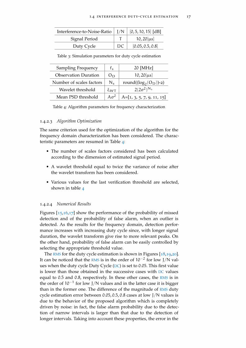
Figures [15,16,17] show the performance of the probability of misseddetection and of the probability of false alarm, when an outlier isdetected. As the results for the frequency domain, detection perfor-mance increases with increasing duty cycle since, with longer signalduration, the wavelet transform give rise to more relevant peaks. Onthe other hand, probability of false alarm can be easily controlled byselecting the appropriate threshold value.
The RMS for the duty cycle estimation is shown in Figures [18,19,20].It can be noticed that the RMS is in the order of 10−2 for low J/N val-ues when the duty cycle Duty Cycle (DC) is set to 0.05. This first valueis lower than those obtained in the successive cases with DC valuesequal to 0.5 and 0.8, respectively. In these other cases, the RMS is inthe order of 10−1 for low J/N values and in the latter case it is biggerthan in the former one. The difference of the magnitude of RMS dutycycle estimation error between 0.05, 0.5, 0.8 cases at low J/N values isdue to the behavior of the proposed algorithm which is completelydriven by noise: in fact, the false alarm probability due to the detec-tion of narrow intervals is larger than that due to the detection oflonger intervals. Taking into account these properties, the error in the
18 interference detection
2 4 6 8 100
0.1
0.2
0.3
0.4
0.5
0.6
0.7
0.8
0.9
1
threshold A
Pm
d,
Pout
Probabilities @ DC = 0.05
Pmd @ J/N=0 [dB]Pmd @ J/N=5 [dB]Pmd @ J/N=10 [dB]Pmd @ J/N=15 [dB]Pout @ J/N=0 [dB]Pout @ J/N=5 [dB]Pout @ J/N=10 [dB]Pout @ J/N=15 [dB]
Figure 15: Pmd,Pout@ Duty Cycle equal to 0.05
2 4 6 8 100
0.1
0.2
0.3
0.4
0.5
0.6
0.7
0.8
0.9
1
threshold A
Pm
d,
Po
ut
Probabilities @ DC = 0.5
Pmd @ J/N=0 [dB]Pmd @ J/N=5 [dB]Pmd @ J/N=10 [dB]Pmd @ J/N=15 [dB]Pout @ J/N=0 [dB]Pout @ J/N=5 [dB]Pout @ J/N=10 [dB]Pout @ J/N=15 [dB]
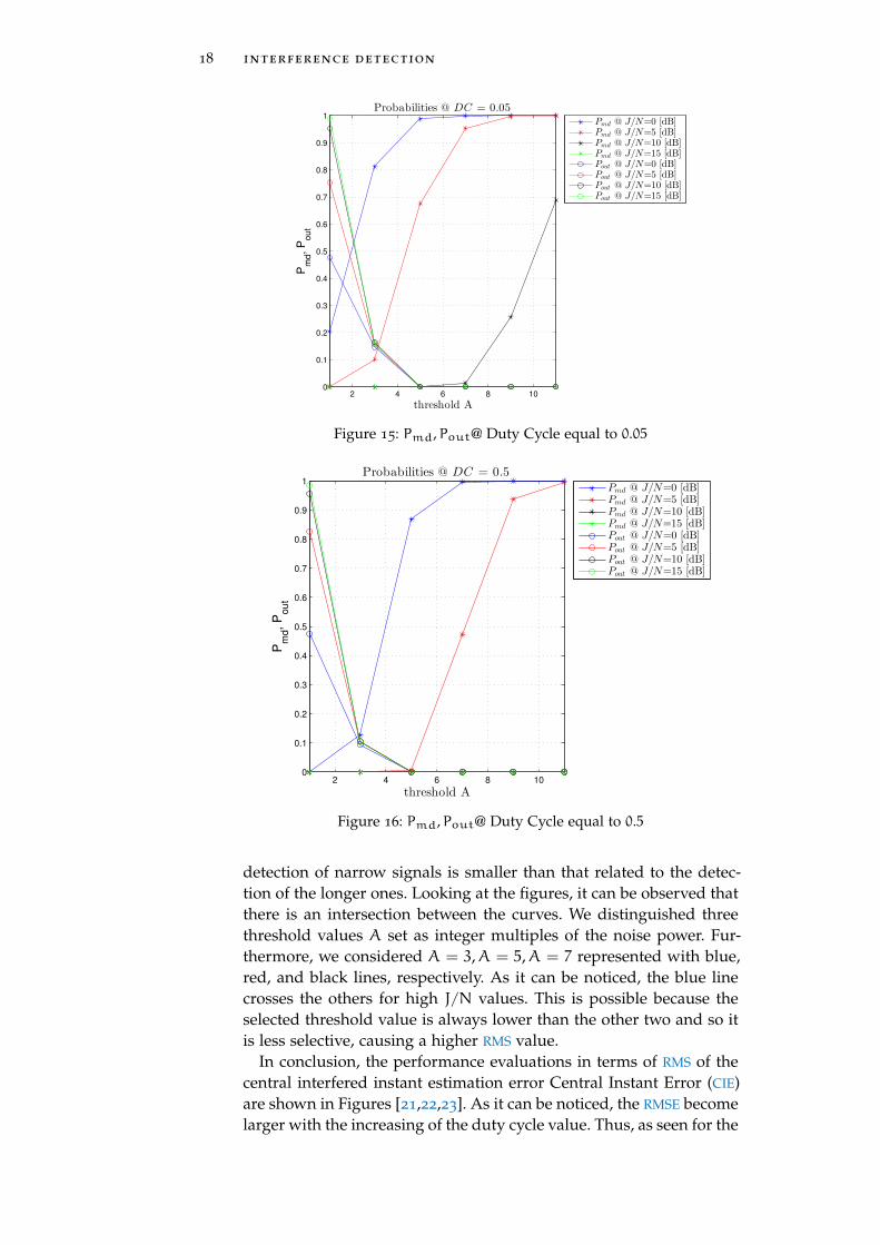
Figure 16: Pmd,Pout@ Duty Cycle equal to 0.5
detection of narrow signals is smaller than that related to the detec-tion of the longer ones. Looking at the figures, it can be observed thatthere is an intersection between the curves. We distinguished threethreshold values A set as integer multiples of the noise power. Fur-thermore, we considered A = 3,A = 5,A = 7 represented with blue,red, and black lines, respectively. As it can be noticed, the blue linecrosses the others for high J/N values. This is possible because theselected threshold value is always lower than the other two and so itis less selective, causing a higher RMS value.
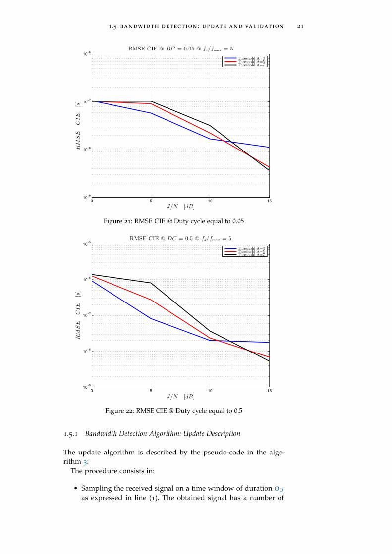
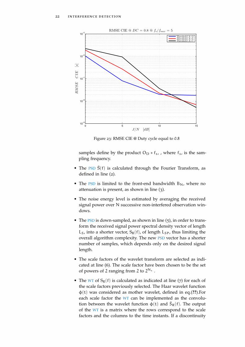
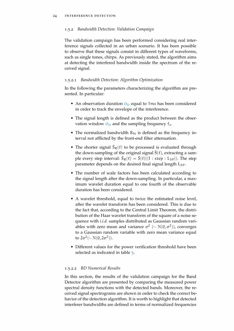
In conclusion, the performance evaluations in terms of RMS of thecentral interfered instant estimation error Central Instant Error (CIE)are shown in Figures [21,22,23]. As it can be noticed, the RMSE becomelarger with the increasing of the duty cycle value. Thus, as seen for the
1.5 bandwidth detection : update and validation 19
2 4 6 8 100
0.1
0.2
0.3
0.4
0.5
0.6
0.7
0.8
0.9
1
threshold A
Pm
d,
Po
ut
Probabilities @ DC = 0.8
Pmd @ J/N=0 [dB]Pmd @ J/N=5 [dB]Pmd @ J/N=10 [dB]Pmd @ J/N=15 [dB]Pout @ J/N=0 [dB]Pout @ J/N=5 [dB]Pout @ J/N=10 [dB]Pout @ J/N=15 [dB]
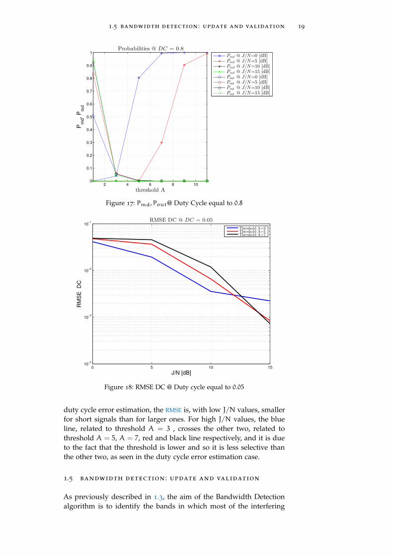
Figure 17: Pmd,Pout@ Duty Cycle equal to 0.8
0 5 10 1510
−4
10−3
10−2
10−1
J/N [dB]
RM
SE
D
C
RMSE DC @ DC = 0.05
Threshold A=3Threshold A=5Threshold A=7
Figure 18: RMSE DC @ Duty cycle equal to 0.05
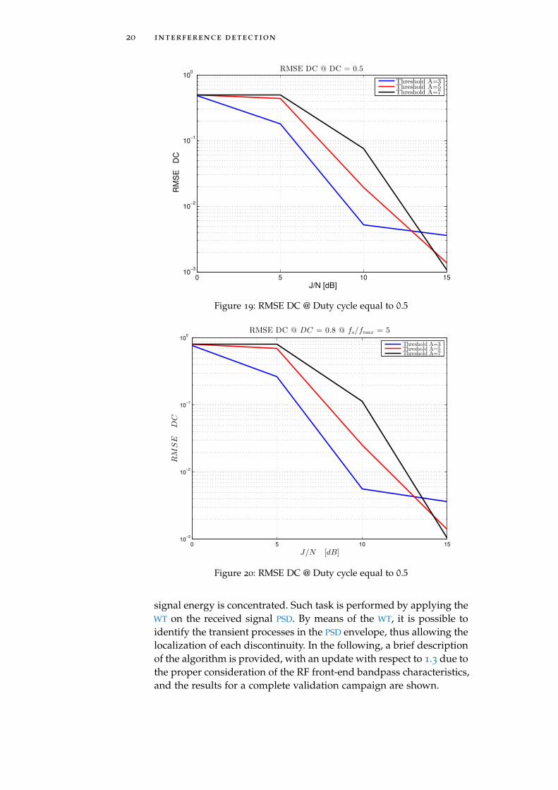
duty cycle error estimation, the RMSE is, with low J/N values, smallerfor short signals than for larger ones. For high J/N values, the blueline, related to threshold A = 3 , crosses the other two, related tothreshold A = 5, A = 7, red and black line respectively, and it is dueto the fact that the threshold is lower and so it is less selective thanthe other two, as seen in the duty cycle error estimation case.
1.5 bandwidth detection : update and validation
As previously described in 1.3, the aim of the Bandwidth Detectionalgorithm is to identify the bands in which most of the interfering
20 interference detection
0 5 10 1510
−3
10−2
10−1
100
J/N [dB]
RM
SE
D
C
RMSE DC @ DC = 0.5
Threshold A=3Threshold A=5Threshold A=7
Figure 19: RMSE DC @ Duty cycle equal to 0.5
0 5 10 1510
−3
10−2
10−1
100
J/N [dB]
RM
SE
DC
RMSE DC @ DC = 0.8 @ fs/fmax = 5
Threshold A=3Threshold A=5Threshold A=7
Figure 20: RMSE DC @ Duty cycle equal to 0.5
signal energy is concentrated. Such task is performed by applying theWT on the received signal PSD. By means of the WT, it is possible toidentify the transient processes in the PSD envelope, thus allowing thelocalization of each discontinuity. In the following, a brief descriptionof the algorithm is provided, with an update with respect to 1.3 due tothe proper consideration of the RF front-end bandpass characteristics,and the results for a complete validation campaign are shown.
1.5 bandwidth detection : update and validation 21
0 5 10 1510
−9
10−8
10−7
10−6
J/N [dB]
RM
SE
CIE
[s]
RMSE CIE @ DC = 0.05 @ fs/fmax = 5
Threshold A=3Threshold A=5Threshold A=7
Figure 21: RMSE CIE @ Duty cycle equal to 0.05
0 5 10 1510
−9
10−8
10−7
10−6
10−5
J/N [dB]
RM
SE
CIE
[s]
RMSE CIE @ DC = 0.5 @ fs/fmax = 5
Threshold A=3Threshold A=5Threshold A=7
Figure 22: RMSE CIE @ Duty cycle equal to 0.5
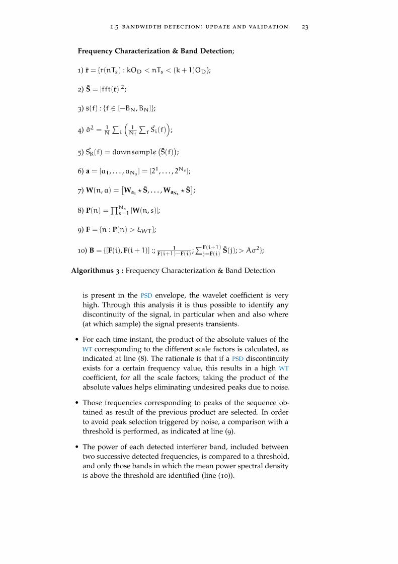
1.5.1 Bandwidth Detection Algorithm: Update Description
The update algorithm is described by the pseudo-code in the algo-rithm 3:
The procedure consists in:
• Sampling the received signal on a time window of duration OD
as expressed in line (1). The obtained signal has a number of
22 interference detection
0 5 10 1510
−9
10−8
10−7
10−6
10−5
J/N [dB]
RM
SE
CIE
[s]
RMSE CIE @ DC = 0.8 @ fs/fmax = 5
Threshold A=3Threshold A=5Threshold A=7
Figure 23: RMSE CIE @ Duty cycle equal to 0.8
samples define by the product OD ∗ fs, , where fs, is the sam-pling frequency.
• The PSD S(f) is calculated through the Fourier Transform, asdefined in line (2).
• The PSD is limited to the front-end bandwidth BN, where noattenuation is present, as shown in line (3).
• The noise energy level is estimated by averaging the receivedsignal power over N successive non-interfered observation win-dows.
• The PSD is down-sampled, as shown in line (5), in order to trans-form the received signal power spectral density vector of lengthLS, into a shorter vector, SR(f), of length LSP, thus limiting theoverall algorithm complexity. The new PSD vector has a shorternumber of samples, which depends only on the desired signallength.
• The scale factors of the wavelet transform are selected as indi-cated at line (6). The scale factor have been chosen to be the setof powers of 2 ranging from 2 to 2Ns .
• The WT of SR(f) is calculated as indicated at line (7) for each ofthe scale factors previously selected. The Haar wavelet functionφ(t) was considered as mother wavelet, defined in eq.(??).Foreach scale factor the WT can be implemented as the convolu-tion between the wavelet function φ(t) and SR(f). The outputof the WT is a matrix where the rows correspond to the scalefactors and the columns to the time instants. If a discontinuity
1.5 bandwidth detection : update and validation 23
Frequency Characterization & Band Detection;;1) r = {r(nTs) : kOD < nTs < (k+ 1)OD};;2) S = |fft(r)|2;;3) s(f) : {f ∈ [−BN,BN]};;
4) σ2 = 1N
∑i
(1Nf
∑f Si(f)
);
;5) SR(f) = downsample
(S(f)
);
;6) a = [a1, . . . ,aNs ] = [21, . . . , 2Ns ];;7) W(n,a) =
[Wa1 ? S, . . . , WaNs
? S];
;8) P(n) =
∏Nss=1 |W(n, s)|;
;9) F = {n : P(n) > ξWT };;
10) B = {[F(i), F(i+ 1)] :; 1F(i+1)−F(i) ;
∑F(i+1)j=F(i) S(j);> Aσ2};
;Algorithmus 3 : Frequency Characterization & Band Detection
is present in the PSD envelope, the wavelet coefficient is veryhigh. Through this analysis it is thus possible to identify anydiscontinuity of the signal, in particular when and also where(at which sample) the signal presents transients.
• For each time instant, the product of the absolute values of theWT corresponding to the different scale factors is calculated, asindicated at line (8). The rationale is that if a PSD discontinuityexists for a certain frequency value, this results in a high WT
coefficient, for all the scale factors; taking the product of theabsolute values helps eliminating undesired peaks due to noise.
• Those frequencies corresponding to peaks of the sequence ob-tained as result of the previous product are selected. In orderto avoid peak selection triggered by noise, a comparison with athreshold is performed, as indicated at line (9).
• The power of each detected interferer band, included betweentwo successive detected frequencies, is compared to a threshold,and only those bands in which the mean power spectral densityis above the threshold are identified (line (10)).
24 interference detection
1.5.2 Bandwidth Detection: Validation Campaign
The validation campaign has been performed considering real inter-ference signals collected in an urban scenario. It has been possibleto observe that these signals consist in different types of waveforms,such as single tones, chirps. As previously stated, the algorithm aimsat detecting the interfered bandwidth inside the spectrum of the re-ceived signal.
1.5.2.1 Bandwidth Detection: Algorithm Optimization
In the following the parameters characterizing the algorithm are pre-sented. In particular:
• An observation duration OD equal to 1ms has been consideredin order to track the envelope of the interference.
• The signal length is defined as the product between the obser-vation window OD and the sampling frequency fs.
• The normalized bandwidth BN is defined as the frequency in-terval not afflicted by the front-end filter attenuation.
• The shorter signal SR(f) to be processed is evaluated throughthe down-sampling of the original signal S(f), extracting a sam-ple every step interval: SR(f) = S(f)([1 : step : LSP]). The stepparameter depends on the desired final signal length LSP.
• The number of scale factors has been calculated according tothe signal length after the down-sampling. In particular, a max-imum wavelet duration equal to one fourth of the observableduration has been considered.
• A wavelet threshold, equal to twice the estimated noise level,after the wavelet transform has been considered. This is due tothe fact that, according to the Central Limit Theorem, the distri-bution of the Haar wavelet transform of the square of a noise se-quence with i.i.d. samples distributed as Gaussian random vari-ables with zero mean and variance σ2 (∼ N(0,σ2)), convergesto a Gaussian random variable with zero mean variance equalto 2σ2(∼ N(0, 2σ2)).
• Different values for the power verification threshold have beenselected as indicated in table 5.
1.5.2.2 BD Numerical Results
In this section, the results of the validation campaign for the BandDetector algorithm are presented by comparing the measured powerspectral density functions with the detected bands. Moreover, the re-ceived signal spectrograms are shown in order to check the correct be-havior of the detection algorithm. It is worth to highlight that detectedinterferer bandwidths are defined in terms of normalized frequencies
1.5 bandwidth detection : update and validation 25
Sampling Frequency fs 16 [MHz]
Observation Duration OD 1[ms]
Signal Length LS 16000 samples
Number of Realizations N 100
Normalized Bandwidth BN [−0.35, 0.35]
Shorter Signal Length LSP 400 samples
Number of scales factors Ns round((log2(LSP)) − 2)
Wavelet threshold ξWT 2(2σ2)Ns
Mean PSD threshold Aσ2 A = [2, 4, 8]
Table 5: Update parameters for frequency characterization
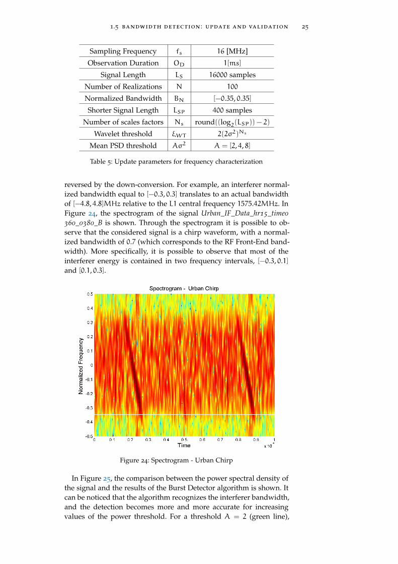
reversed by the down-conversion. For example, an interferer normal-ized bandwidth equal to [−0.3, 0.3] translates to an actual bandwidthof [−4.8, 4.8]MHz relative to the L1 central frequency 1575.42MHz. InFigure 24, the spectrogram of the signal Urban_IF_Data_hr15_time0360_0380_B is shown. Through the spectrogram it is possible to ob-serve that the considered signal is a chirp waveform, with a normal-ized bandwidth of 0.7 (which corresponds to the RF Front-End band-width). More specifically, it is possible to observe that most of theinterferer energy is contained in two frequency intervals, [−0.3, 0.1]and [0.1, 0.3].
Figure 24: Spectrogram - Urban Chirp
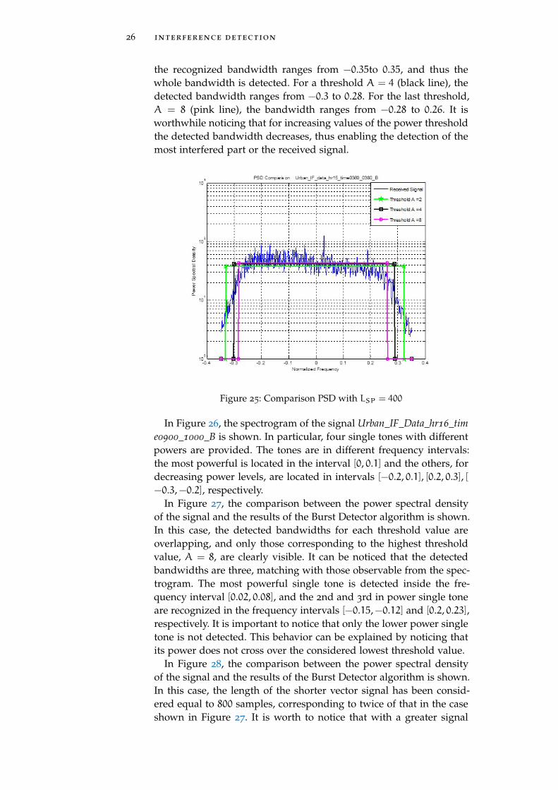
In Figure 25, the comparison between the power spectral density ofthe signal and the results of the Burst Detector algorithm is shown. Itcan be noticed that the algorithm recognizes the interferer bandwidth,and the detection becomes more and more accurate for increasingvalues of the power threshold. For a threshold A = 2 (green line),
26 interference detection
the recognized bandwidth ranges from −0.35to 0.35, and thus thewhole bandwidth is detected. For a threshold A = 4 (black line), thedetected bandwidth ranges from −0.3 to 0.28. For the last threshold,A = 8 (pink line), the bandwidth ranges from −0.28 to 0.26. It isworthwhile noticing that for increasing values of the power thresholdthe detected bandwidth decreases, thus enabling the detection of themost interfered part or the received signal.
Figure 25: Comparison PSD with LSP = 400
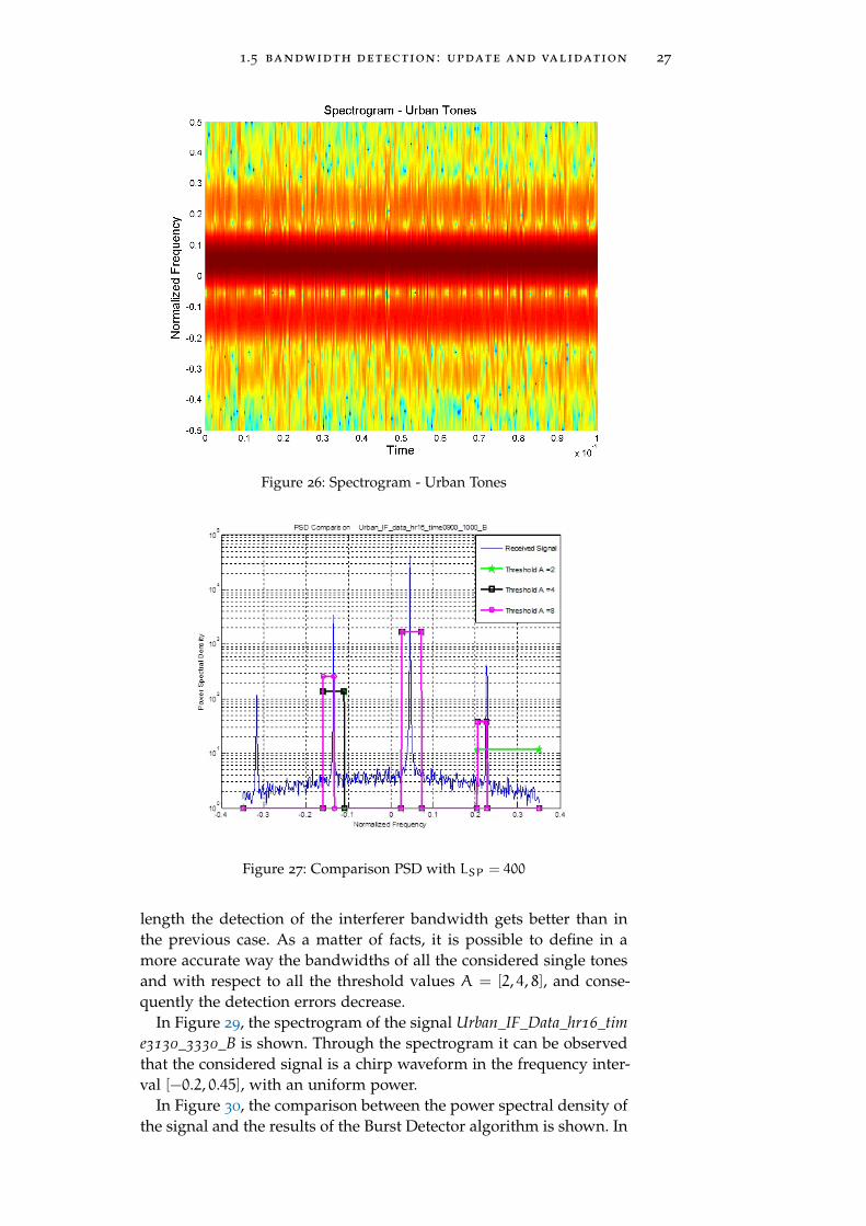
In Figure 26, the spectrogram of the signal Urban_IF_Data_hr16_time0900_1000_B is shown. In particular, four single tones with differentpowers are provided. The tones are in different frequency intervals:the most powerful is located in the interval [0, 0.1] and the others, fordecreasing power levels, are located in intervals [−0.2, 0.1], [0.2, 0.3], [−0.3,−0.2], respectively.
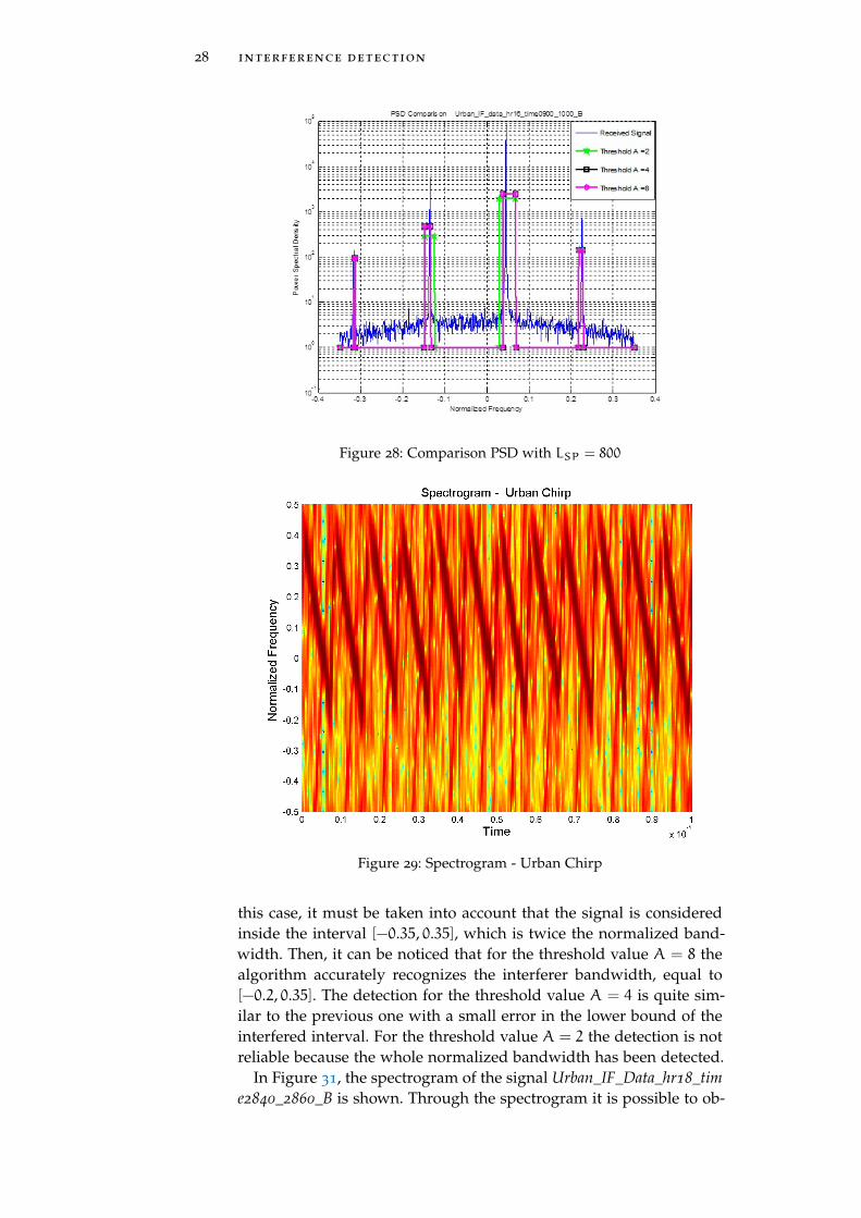
In Figure 27, the comparison between the power spectral densityof the signal and the results of the Burst Detector algorithm is shown.In this case, the detected bandwidths for each threshold value areoverlapping, and only those corresponding to the highest thresholdvalue, A = 8, are clearly visible. It can be noticed that the detectedbandwidths are three, matching with those observable from the spec-trogram. The most powerful single tone is detected inside the fre-quency interval [0.02, 0.08], and the 2nd and 3rd in power single toneare recognized in the frequency intervals [−0.15,−0.12] and [0.2, 0.23],respectively. It is important to notice that only the lower power singletone is not detected. This behavior can be explained by noticing thatits power does not cross over the considered lowest threshold value.
In Figure 28, the comparison between the power spectral densityof the signal and the results of the Burst Detector algorithm is shown.In this case, the length of the shorter vector signal has been consid-ered equal to 800 samples, corresponding to twice of that in the caseshown in Figure 27. It is worth to notice that with a greater signal
1.5 bandwidth detection : update and validation 27
Figure 26: Spectrogram - Urban Tones
Figure 27: Comparison PSD with LSP = 400
length the detection of the interferer bandwidth gets better than inthe previous case. As a matter of facts, it is possible to define in amore accurate way the bandwidths of all the considered single tonesand with respect to all the threshold values A = [2, 4, 8], and conse-quently the detection errors decrease.
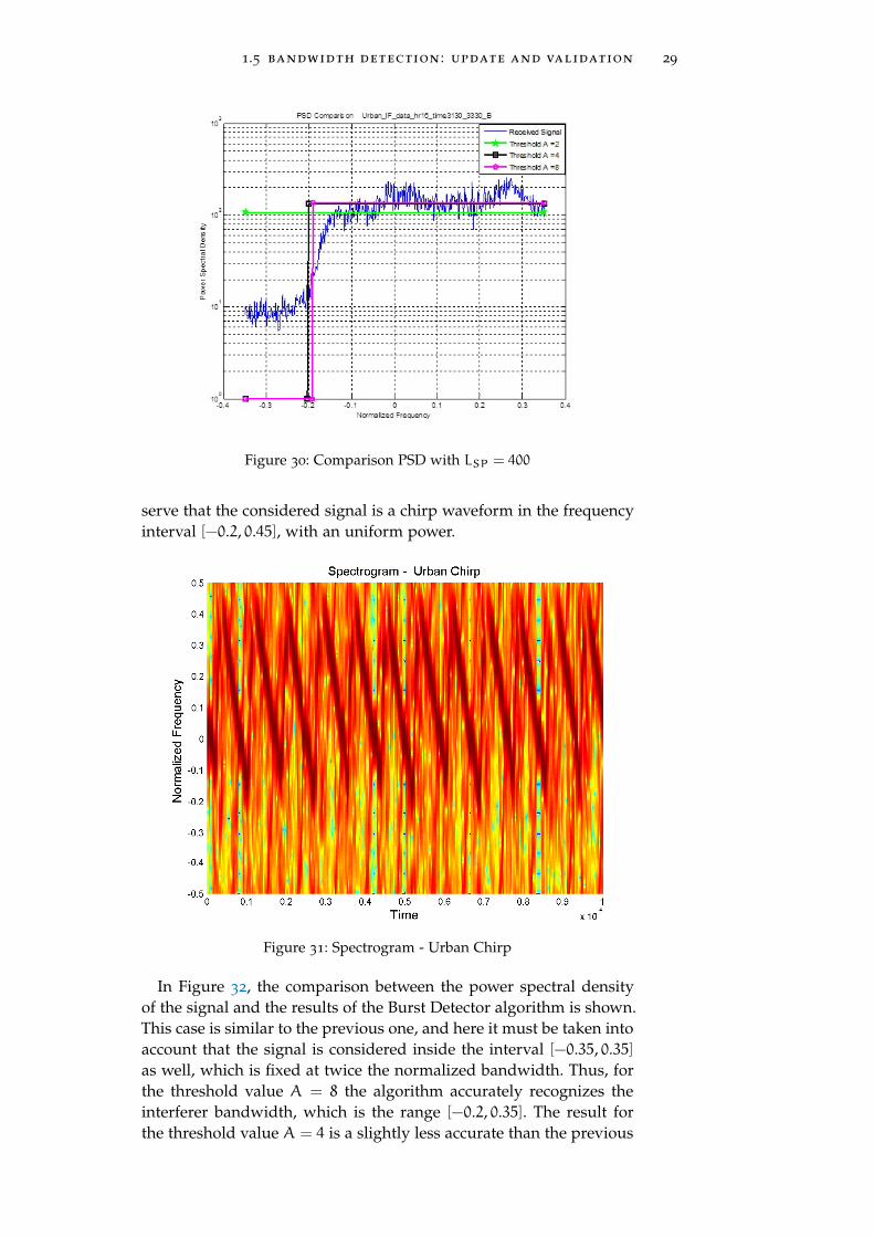
In Figure 29, the spectrogram of the signal Urban_IF_Data_hr16_time3130_3330_B is shown. Through the spectrogram it can be observedthat the considered signal is a chirp waveform in the frequency inter-val [−0.2, 0.45], with an uniform power.
In Figure 30, the comparison between the power spectral density ofthe signal and the results of the Burst Detector algorithm is shown. In
28 interference detection
Figure 28: Comparison PSD with LSP = 800
Figure 29: Spectrogram - Urban Chirp
this case, it must be taken into account that the signal is consideredinside the interval [−0.35, 0.35], which is twice the normalized band-width. Then, it can be noticed that for the threshold value A = 8 thealgorithm accurately recognizes the interferer bandwidth, equal to[−0.2, 0.35]. The detection for the threshold value A = 4 is quite sim-ilar to the previous one with a small error in the lower bound of theinterfered interval. For the threshold value A = 2 the detection is notreliable because the whole normalized bandwidth has been detected.
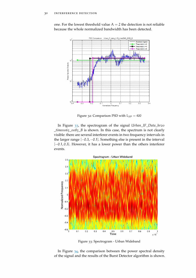
In Figure 31, the spectrogram of the signal Urban_IF_Data_hr18_time2840_2860_B is shown. Through the spectrogram it is possible to ob-
1.5 bandwidth detection : update and validation 29
Figure 30: Comparison PSD with LSP = 400
serve that the considered signal is a chirp waveform in the frequencyinterval [−0.2, 0.45], with an uniform power.
Figure 31: Spectrogram - Urban Chirp
In Figure 32, the comparison between the power spectral densityof the signal and the results of the Burst Detector algorithm is shown.This case is similar to the previous one, and here it must be taken intoaccount that the signal is considered inside the interval [−0.35, 0.35]as well, which is fixed at twice the normalized bandwidth. Thus, forthe threshold value A = 8 the algorithm accurately recognizes theinterferer bandwidth, which is the range [−0.2, 0.35]. The result forthe threshold value A = 4 is a slightly less accurate than the previous
30 interference detection
one. For the lowest threshold value A = 2 the detection is not reliablebecause the whole normalized bandwidth has been detected.
Figure 32: Comparison PSD with LSP = 400
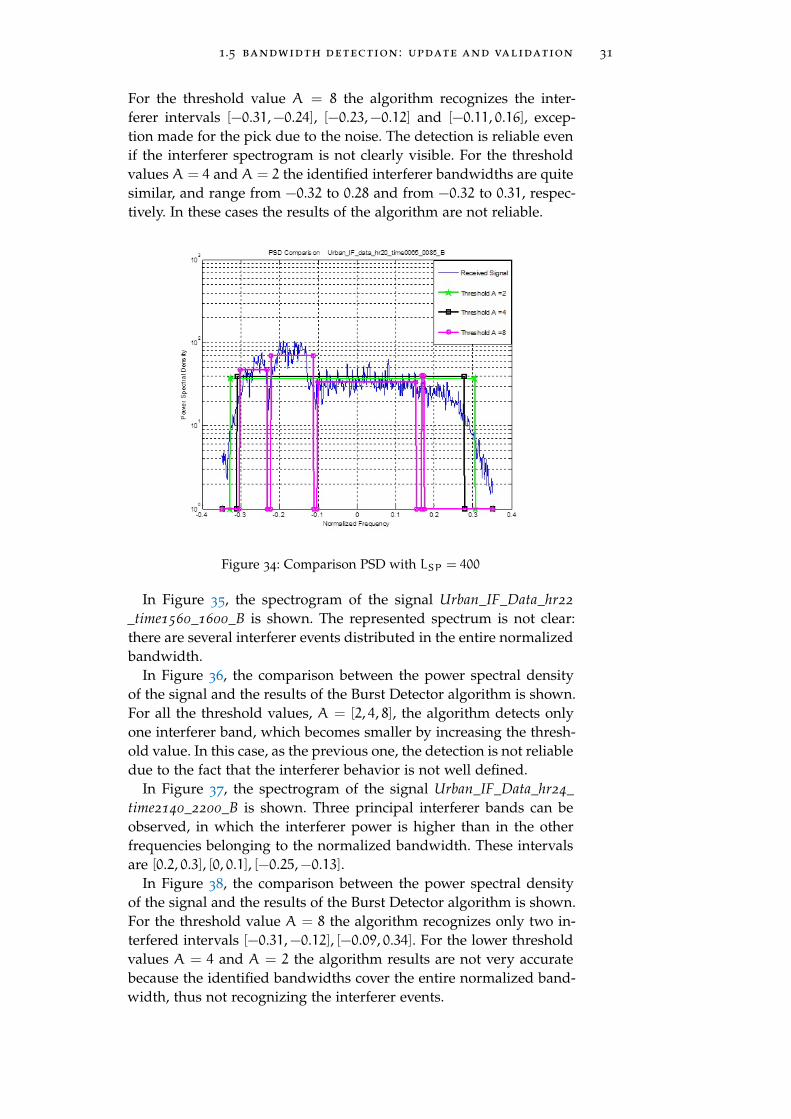
In Figure 33, the spectrogram of the signal Urban_IF_Data_hr20_time0065_0085_B is shown. In this case, the spectrum is not clearlyvisible: there are several interferer events in two frequency intervals inthe larger range [−0.3,−0.1]. Something else is present in the interval[−0.1, 0.3]. However, it has a lower power than the others interfererevents.
Figure 33: Spectrogram - Urban Wideband
In Figure 34, the comparison between the power spectral densityof the signal and the results of the Burst Detector algorithm is shown.
1.5 bandwidth detection : update and validation 31
For the threshold value A = 8 the algorithm recognizes the inter-ferer intervals [−0.31,−0.24], [−0.23,−0.12] and [−0.11, 0.16], excep-tion made for the pick due to the noise. The detection is reliable evenif the interferer spectrogram is not clearly visible. For the thresholdvalues A = 4 and A = 2 the identified interferer bandwidths are quitesimilar, and range from −0.32 to 0.28 and from −0.32 to 0.31, respec-tively. In these cases the results of the algorithm are not reliable.
Figure 34: Comparison PSD with LSP = 400
In Figure 35, the spectrogram of the signal Urban_IF_Data_hr22_time1560_1600_B is shown. The represented spectrum is not clear:there are several interferer events distributed in the entire normalizedbandwidth.
In Figure 36, the comparison between the power spectral densityof the signal and the results of the Burst Detector algorithm is shown.For all the threshold values, A = [2, 4, 8], the algorithm detects onlyone interferer band, which becomes smaller by increasing the thresh-old value. In this case, as the previous one, the detection is not reliabledue to the fact that the interferer behavior is not well defined.
In Figure 37, the spectrogram of the signal Urban_IF_Data_hr24_time2140_2200_B is shown. Three principal interferer bands can beobserved, in which the interferer power is higher than in the otherfrequencies belonging to the normalized bandwidth. These intervalsare [0.2, 0.3], [0, 0.1], [−0.25,−0.13].
In Figure 38, the comparison between the power spectral densityof the signal and the results of the Burst Detector algorithm is shown.For the threshold value A = 8 the algorithm recognizes only two in-terfered intervals [−0.31,−0.12], [−0.09, 0.34]. For the lower thresholdvalues A = 4 and A = 2 the algorithm results are not very accuratebecause the identified bandwidths cover the entire normalized band-width, thus not recognizing the interferer events.
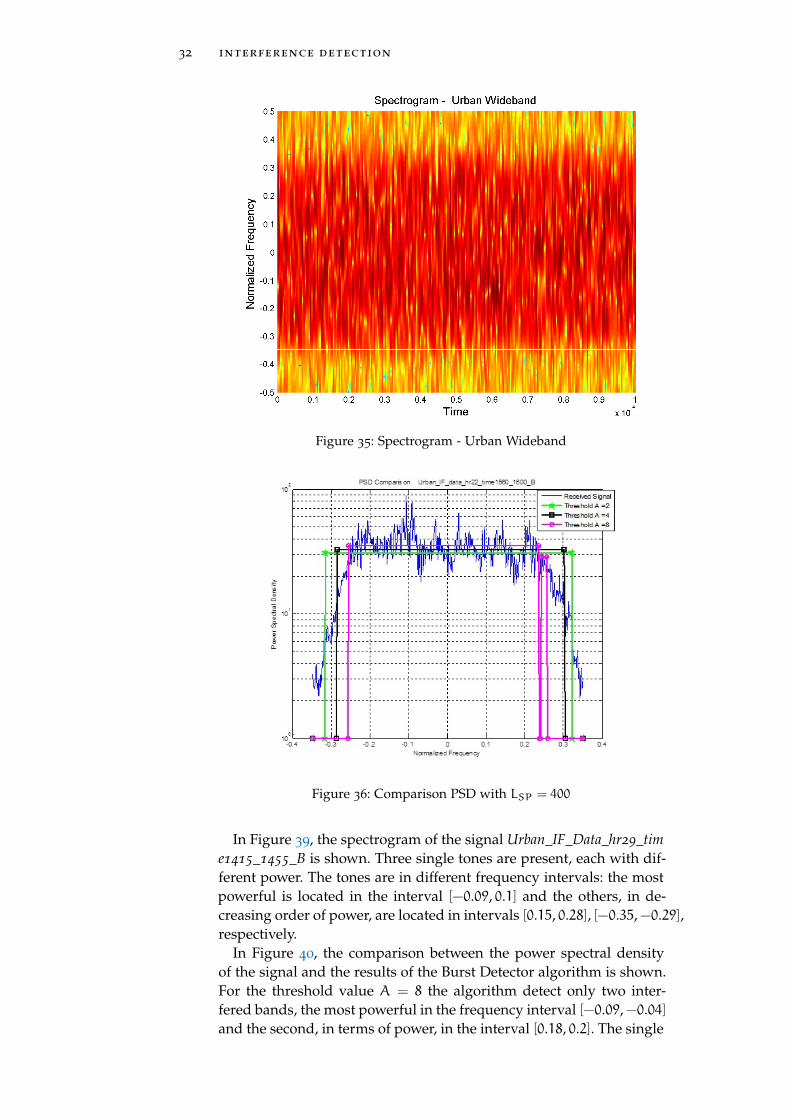
32 interference detection
Figure 35: Spectrogram - Urban Wideband
Figure 36: Comparison PSD with LSP = 400
In Figure 39, the spectrogram of the signal Urban_IF_Data_hr29_time1415_1455_B is shown. Three single tones are present, each with dif-ferent power. The tones are in different frequency intervals: the mostpowerful is located in the interval [−0.09, 0.1] and the others, in de-creasing order of power, are located in intervals [0.15, 0.28], [−0.35,−0.29],respectively.
In Figure 40, the comparison between the power spectral densityof the signal and the results of the Burst Detector algorithm is shown.For the threshold value A = 8 the algorithm detect only two inter-fered bands, the most powerful in the frequency interval [−0.09,−0.04]and the second, in terms of power, in the interval [0.18, 0.2]. The single
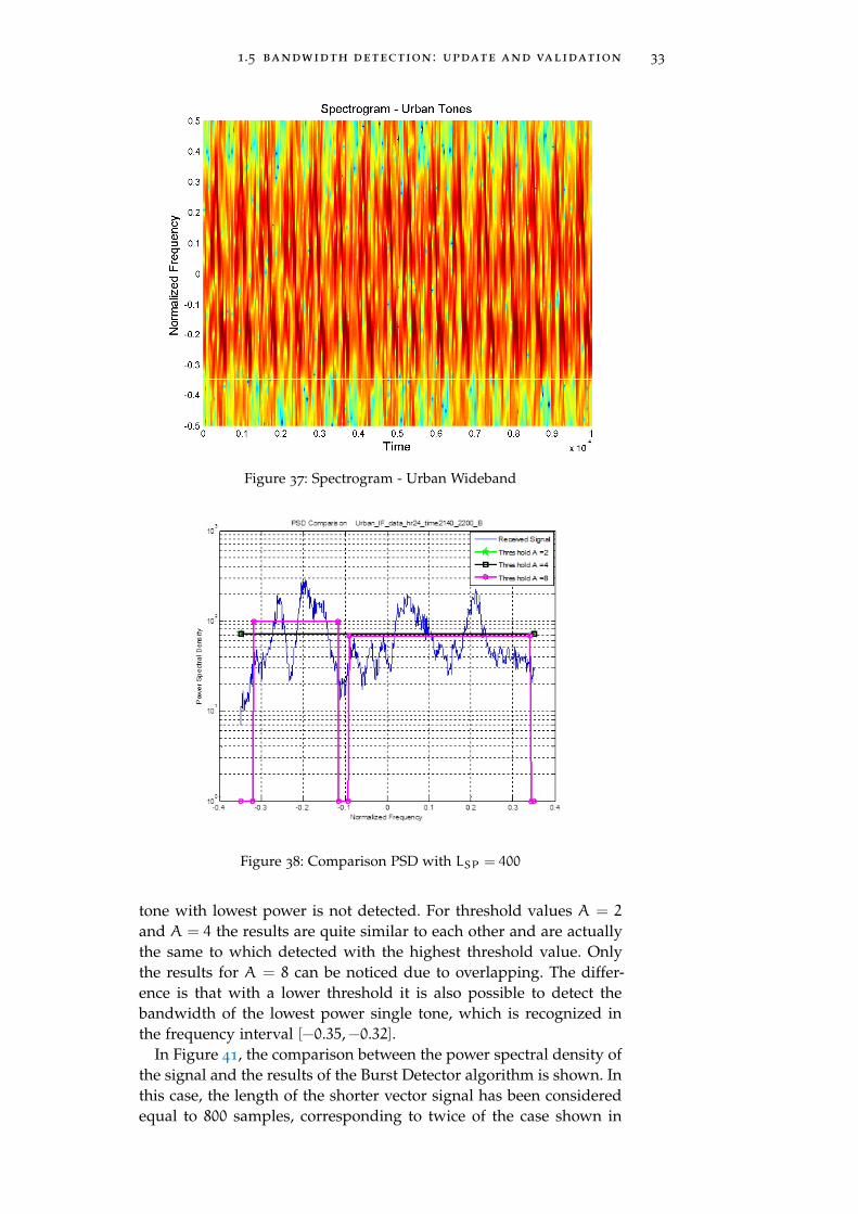
1.5 bandwidth detection : update and validation 33
Figure 37: Spectrogram - Urban Wideband
Figure 38: Comparison PSD with LSP = 400
tone with lowest power is not detected. For threshold values A = 2
and A = 4 the results are quite similar to each other and are actuallythe same to which detected with the highest threshold value. Onlythe results for A = 8 can be noticed due to overlapping. The differ-ence is that with a lower threshold it is also possible to detect thebandwidth of the lowest power single tone, which is recognized inthe frequency interval [−0.35,−0.32].
In Figure 41, the comparison between the power spectral density ofthe signal and the results of the Burst Detector algorithm is shown. Inthis case, the length of the shorter vector signal has been consideredequal to 800 samples, corresponding to twice of the case shown in
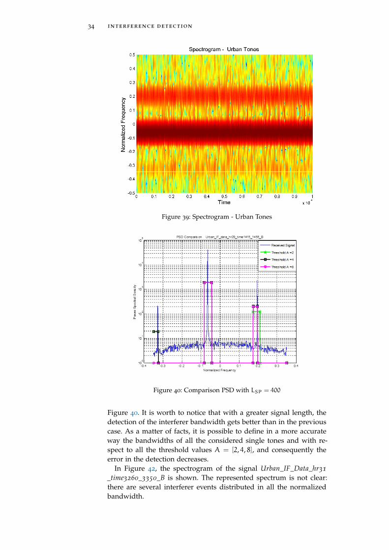
34 interference detection
Figure 39: Spectrogram - Urban Tones
Figure 40: Comparison PSD with LSP = 400
Figure 40. It is worth to notice that with a greater signal length, thedetection of the interferer bandwidth gets better than in the previouscase. As a matter of facts, it is possible to define in a more accurateway the bandwidths of all the considered single tones and with re-spect to all the threshold values A = [2, 4, 8], and consequently theerror in the detection decreases.
In Figure 42, the spectrogram of the signal Urban_IF_Data_hr31_time3260_3350_B is shown. The represented spectrum is not clear:there are several interferer events distributed in all the normalizedbandwidth.
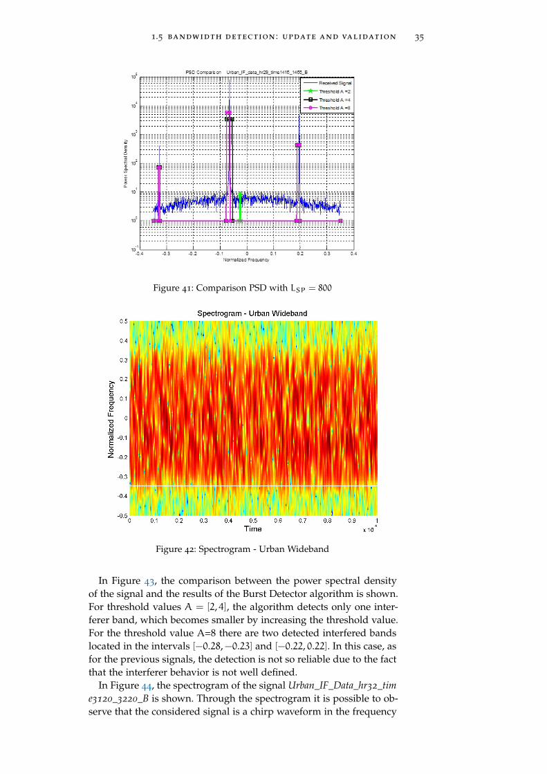
1.5 bandwidth detection : update and validation 35
Figure 41: Comparison PSD with LSP = 800
Figure 42: Spectrogram - Urban Wideband
In Figure 43, the comparison between the power spectral densityof the signal and the results of the Burst Detector algorithm is shown.For threshold values A = [2, 4], the algorithm detects only one inter-ferer band, which becomes smaller by increasing the threshold value.For the threshold value A=8 there are two detected interfered bandslocated in the intervals [−0.28,−0.23] and [−0.22, 0.22]. In this case, asfor the previous signals, the detection is not so reliable due to the factthat the interferer behavior is not well defined.
In Figure 44, the spectrogram of the signal Urban_IF_Data_hr32_time3120_3220_B is shown. Through the spectrogram it is possible to ob-serve that the considered signal is a chirp waveform in the frequency
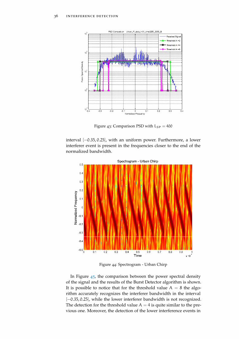
36 interference detection
Figure 43: Comparison PSD with LSP = 400
interval [−0.35, 0.25], with an uniform power. Furthermore, a lowerinterferer event is present in the frequencies closer to the end of thenormalized bandwidth.
Figure 44: Spectrogram - Urban Chirp
In Figure 45, the comparison between the power spectral densityof the signal and the results of the Burst Detector algorithm is shown.It is possible to notice that for the threshold value A = 8 the algo-rithm accurately recognizes the interferer bandwidth in the interval[−0.35, 0.25], while the lower interferer bandwidth is not recognized.The detection for the threshold value A = 4 is quite similar to the pre-vious one. Moreover, the detection of the lower interference events in
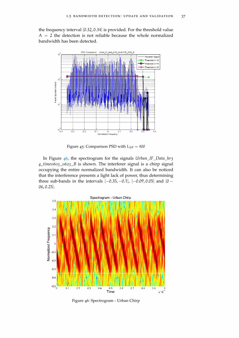
1.5 bandwidth detection : update and validation 37
the frequency interval [0.32, 0.34] is provided. For the threshold valueA = 2 the detection is not reliable because the whole normalizedbandwidth has been detected.
Figure 45: Comparison PSD with LSP = 400
In Figure 46, the spectrogram for the signals Urban_IF_Data_hr34_time0605_0625_B is shown. The interferer signal is a chirp signaloccupying the entire normalized bandwidth. It can also be noticedthat the interference presents a light lack of power, thus determiningthree sub-bands in the intervals [−0.35,−0.1], [−0.09, 0.05] and [0 −
06, 0.25].
Figure 46: Spectrogram - Urban Chirp
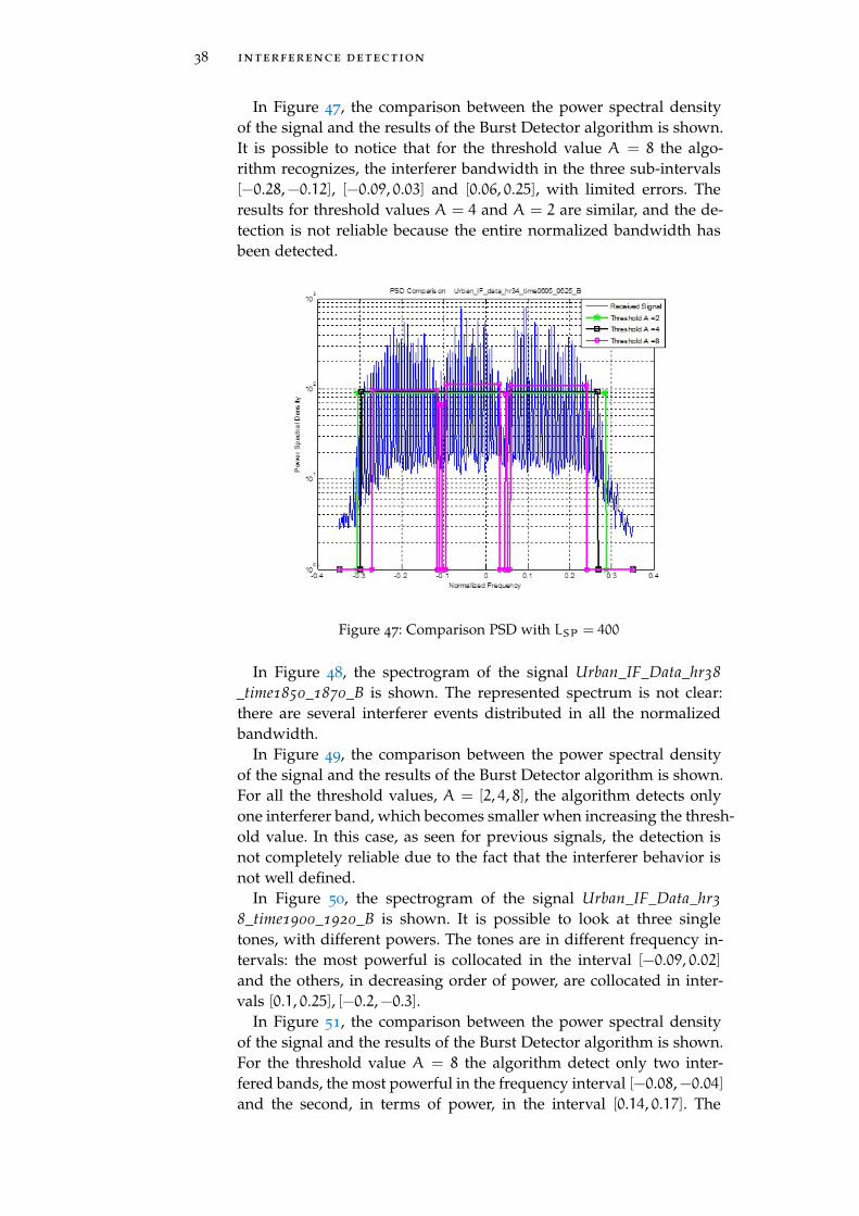
38 interference detection
In Figure 47, the comparison between the power spectral densityof the signal and the results of the Burst Detector algorithm is shown.It is possible to notice that for the threshold value A = 8 the algo-rithm recognizes, the interferer bandwidth in the three sub-intervals[−0.28,−0.12], [−0.09, 0.03] and [0.06, 0.25], with limited errors. Theresults for threshold values A = 4 and A = 2 are similar, and the de-tection is not reliable because the entire normalized bandwidth hasbeen detected.
Figure 47: Comparison PSD with LSP = 400
In Figure 48, the spectrogram of the signal Urban_IF_Data_hr38_time1850_1870_B is shown. The represented spectrum is not clear:there are several interferer events distributed in all the normalizedbandwidth.
In Figure 49, the comparison between the power spectral densityof the signal and the results of the Burst Detector algorithm is shown.For all the threshold values, A = [2, 4, 8], the algorithm detects onlyone interferer band, which becomes smaller when increasing the thresh-old value. In this case, as seen for previous signals, the detection isnot completely reliable due to the fact that the interferer behavior isnot well defined.
In Figure 50, the spectrogram of the signal Urban_IF_Data_hr38_time1900_1920_B is shown. It is possible to look at three singletones, with different powers. The tones are in different frequency in-tervals: the most powerful is collocated in the interval [−0.09, 0.02]and the others, in decreasing order of power, are collocated in inter-vals [0.1, 0.25], [−0.2,−0.3].
In Figure 51, the comparison between the power spectral densityof the signal and the results of the Burst Detector algorithm is shown.For the threshold value A = 8 the algorithm detect only two inter-fered bands, the most powerful in the frequency interval [−0.08,−0.04]and the second, in terms of power, in the interval [0.14, 0.17]. The
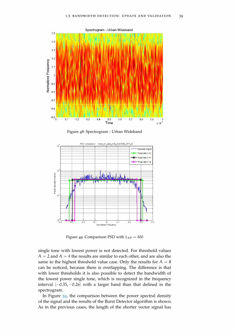
1.5 bandwidth detection : update and validation 39
Figure 48: Spectrogram - Urban Wideband
Figure 49: Comparison PSD with LSP = 400
single tone with lowest power is not detected. For threshold valuesA = 2 and A = 4 the results are similar to each other, and are also thesame to the highest threshold value case. Only the results for A = 8
can be noticed, because there is overlapping. The difference is thatwith lower thresholds it is also possible to detect the bandwidth ofthe lowest power single tone, which is recognized in the frequencyinterval [−0.35,−0.26] with a larger band than that defined in thespectrogram.
In Figure 52, the comparison between the power spectral densityof the signal and the results of the Burst Detector algorithm is shown.As in the previous cases, the length of the shorter vector signal has
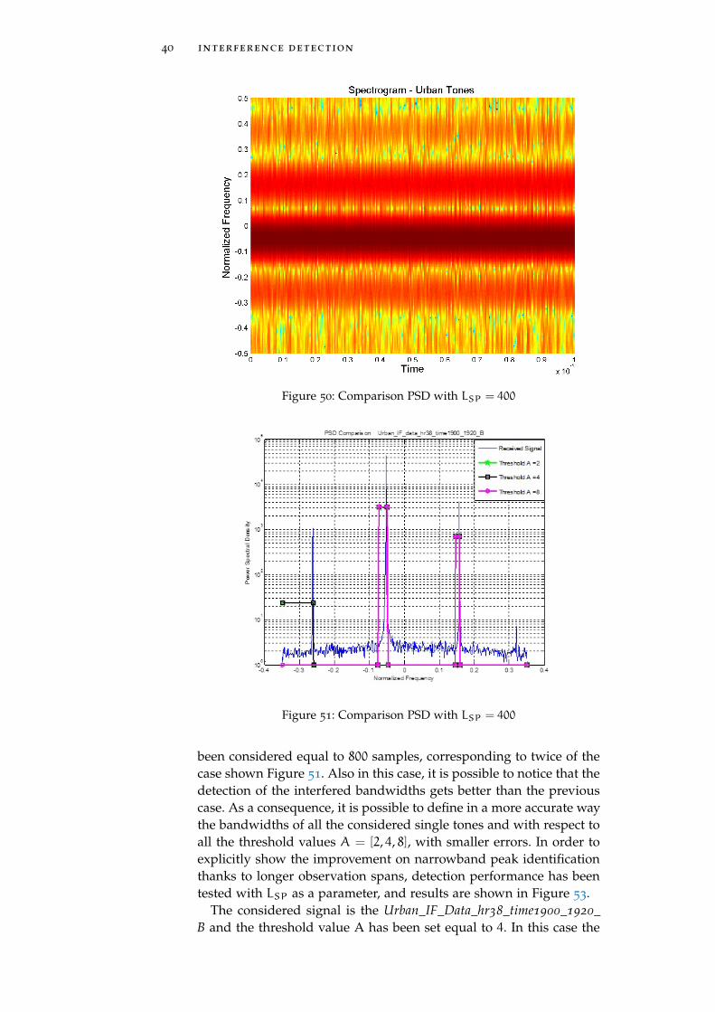
40 interference detection
Figure 50: Comparison PSD with LSP = 400
Figure 51: Comparison PSD with LSP = 400
been considered equal to 800 samples, corresponding to twice of thecase shown Figure 51. Also in this case, it is possible to notice that thedetection of the interfered bandwidths gets better than the previouscase. As a consequence, it is possible to define in a more accurate waythe bandwidths of all the considered single tones and with respect toall the threshold values A = [2, 4, 8], with smaller errors. In order toexplicitly show the improvement on narrowband peak identificationthanks to longer observation spans, detection performance has beentested with LSP as a parameter, and results are shown in Figure 53.
The considered signal is the Urban_IF_Data_hr38_time1900_1920_B and the threshold value A has been set equal to 4. In this case the
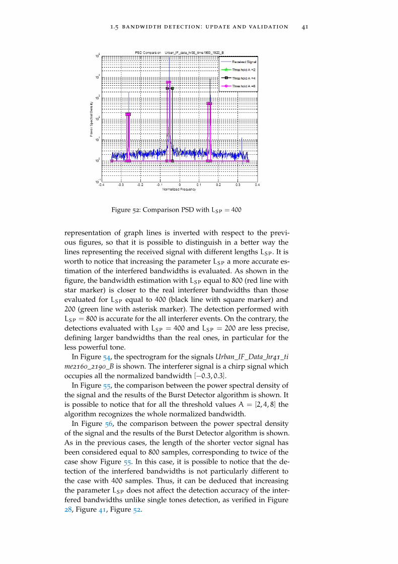
1.5 bandwidth detection : update and validation 41
Figure 52: Comparison PSD with LSP = 400
representation of graph lines is inverted with respect to the previ-ous figures, so that it is possible to distinguish in a better way thelines representing the received signal with different lengths LSP. It isworth to notice that increasing the parameter LSP a more accurate es-timation of the interfered bandwidths is evaluated. As shown in thefigure, the bandwidth estimation with LSP equal to 800 (red line withstar marker) is closer to the real interferer bandwidths than thoseevaluated for LSP equal to 400 (black line with square marker) and200 (green line with asterisk marker). The detection performed withLSP = 800 is accurate for the all interferer events. On the contrary, thedetections evaluated with LSP = 400 and LSP = 200 are less precise,defining larger bandwidths than the real ones, in particular for theless powerful tone.
In Figure 54, the spectrogram for the signals Urban_IF_Data_hr41_time2160_2190_B is shown. The interferer signal is a chirp signal whichoccupies all the normalized bandwidth [−0.3, 0.3].
In Figure 55, the comparison between the power spectral density ofthe signal and the results of the Burst Detector algorithm is shown. Itis possible to notice that for all the threshold values A = [2, 4, 8] thealgorithm recognizes the whole normalized bandwidth.
In Figure 56, the comparison between the power spectral densityof the signal and the results of the Burst Detector algorithm is shown.As in the previous cases, the length of the shorter vector signal hasbeen considered equal to 800 samples, corresponding to twice of thecase show Figure 55. In this case, it is possible to notice that the de-tection of the interfered bandwidths is not particularly different tothe case with 400 samples. Thus, it can be deduced that increasingthe parameter LSP does not affect the detection accuracy of the inter-fered bandwidths unlike single tones detection, as verified in Figure28, Figure 41, Figure 52.
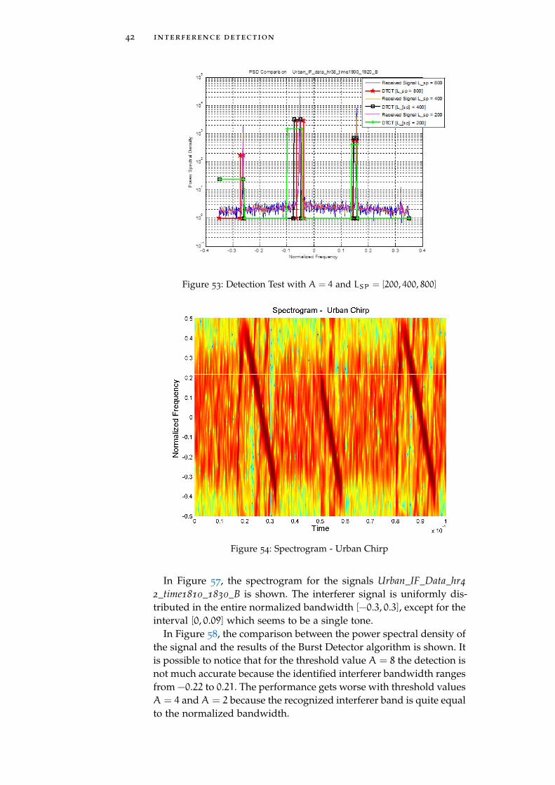
42 interference detection
Figure 53: Detection Test with A = 4 and LSP = [200, 400, 800]
Figure 54: Spectrogram - Urban Chirp
In Figure 57, the spectrogram for the signals Urban_IF_Data_hr42_time1810_1830_B is shown. The interferer signal is uniformly dis-tributed in the entire normalized bandwidth [−0.3, 0.3], except for theinterval [0, 0.09] which seems to be a single tone.
In Figure 58, the comparison between the power spectral density ofthe signal and the results of the Burst Detector algorithm is shown. Itis possible to notice that for the threshold value A = 8 the detection isnot much accurate because the identified interferer bandwidth rangesfrom −0.22 to 0.21. The performance gets worse with threshold valuesA = 4 andA = 2 because the recognized interferer band is quite equalto the normalized bandwidth.
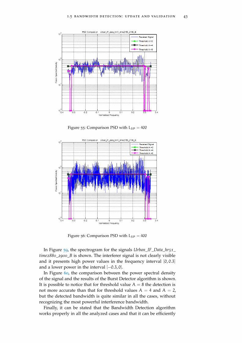
1.5 bandwidth detection : update and validation 43
Figure 55: Comparison PSD with LSP = 400
Figure 56: Comparison PSD with LSP = 400
In Figure 59, the spectrogram for the signals Urban_IF_Data_hr51_time2880_2900_B is shown. The interferer signal is not clearly visibleand it presents high power values in the frequency interval [0, 0.3]and a lower power in the interval [−0.3, 0].
In Figure 60, the comparison between the power spectral densityof the signal and the results of the Burst Detector algorithm is shown.It is possible to notice that for threshold value A = 8 the detection isnot more accurate than that for threshold values A = 4 and A = 2,but the detected bandwidth is quite similar in all the cases, withoutrecognizing the most powerful interference bandwidth.
Finally, it can be stated that the Bandwidth Detection algorithmworks properly in all the analyzed cases and that it can be efficiently
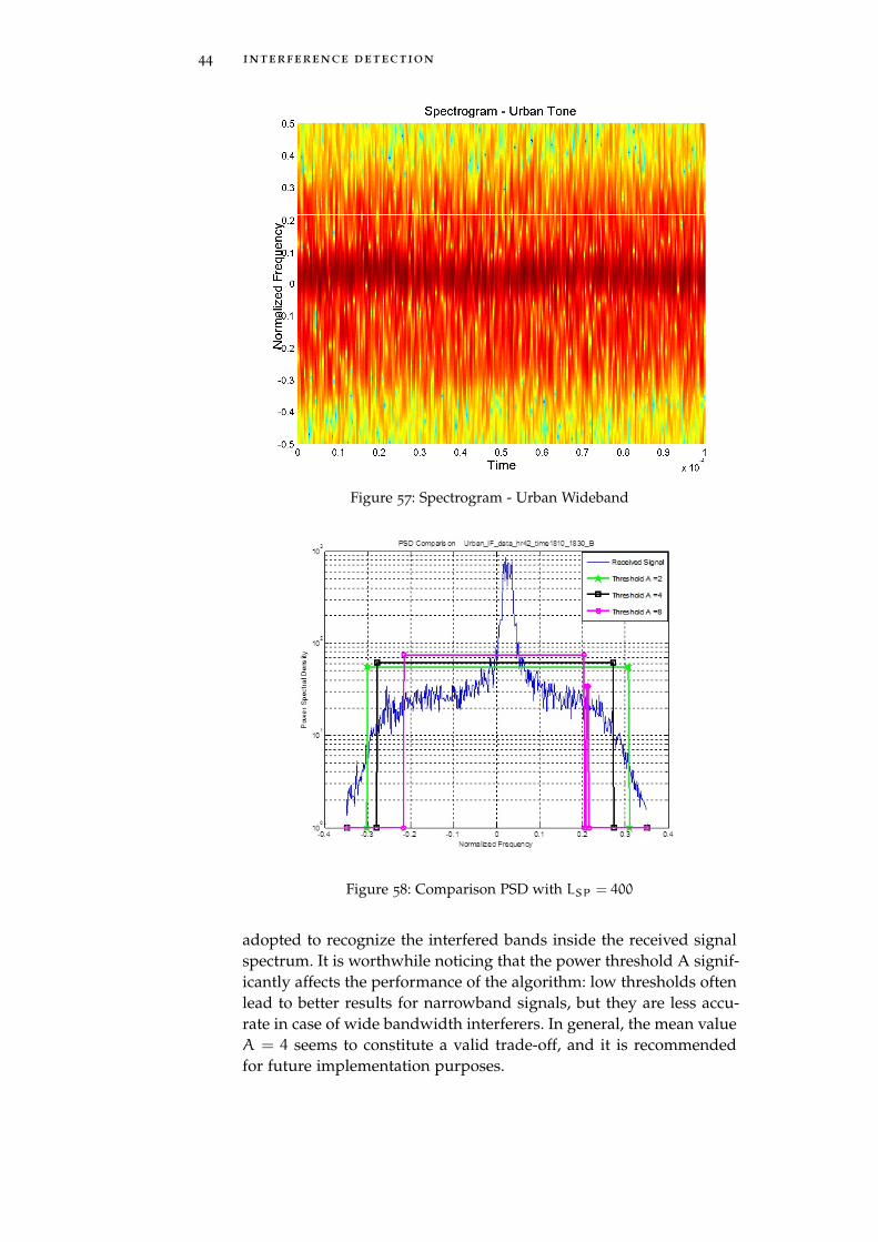
44 interference detection
Figure 57: Spectrogram - Urban Wideband
Figure 58: Comparison PSD with LSP = 400
adopted to recognize the interfered bands inside the received signalspectrum. It is worthwhile noticing that the power threshold A signif-icantly affects the performance of the algorithm: low thresholds oftenlead to better results for narrowband signals, but they are less accu-rate in case of wide bandwidth interferers. In general, the mean valueA = 4 seems to constitute a valid trade-off, and it is recommendedfor future implementation purposes.
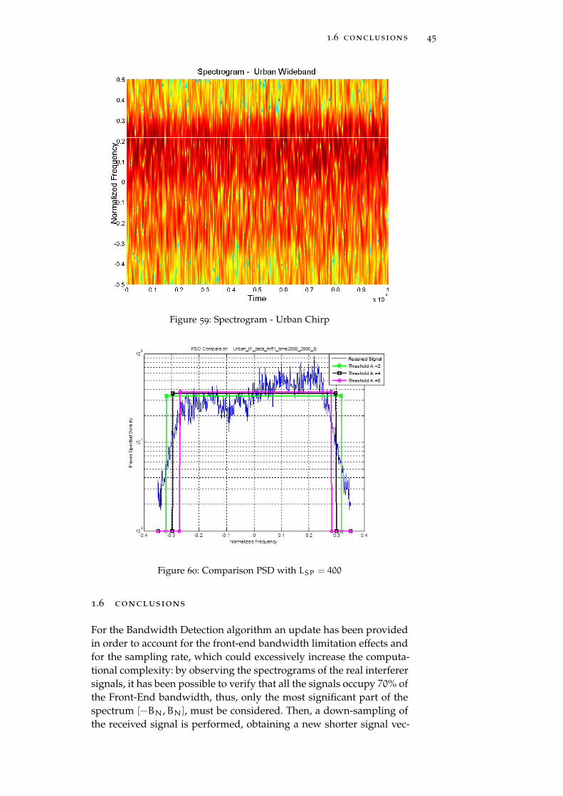
1.6 conclusions 45
Figure 59: Spectrogram - Urban Chirp
Figure 60: Comparison PSD with LSP = 400
1.6 conclusions
For the Bandwidth Detection algorithm an update has been providedin order to account for the front-end bandwidth limitation effects andfor the sampling rate, which could excessively increase the computa-tional complexity: by observing the spectrograms of the real interferersignals, it has been possible to verify that all the signals occupy 70% ofthe Front-End bandwidth, thus, only the most significant part of thespectrum [−BN,BN], must be considered. Then, a down-sampling ofthe received signal is performed, obtaining a new shorter signal vec-
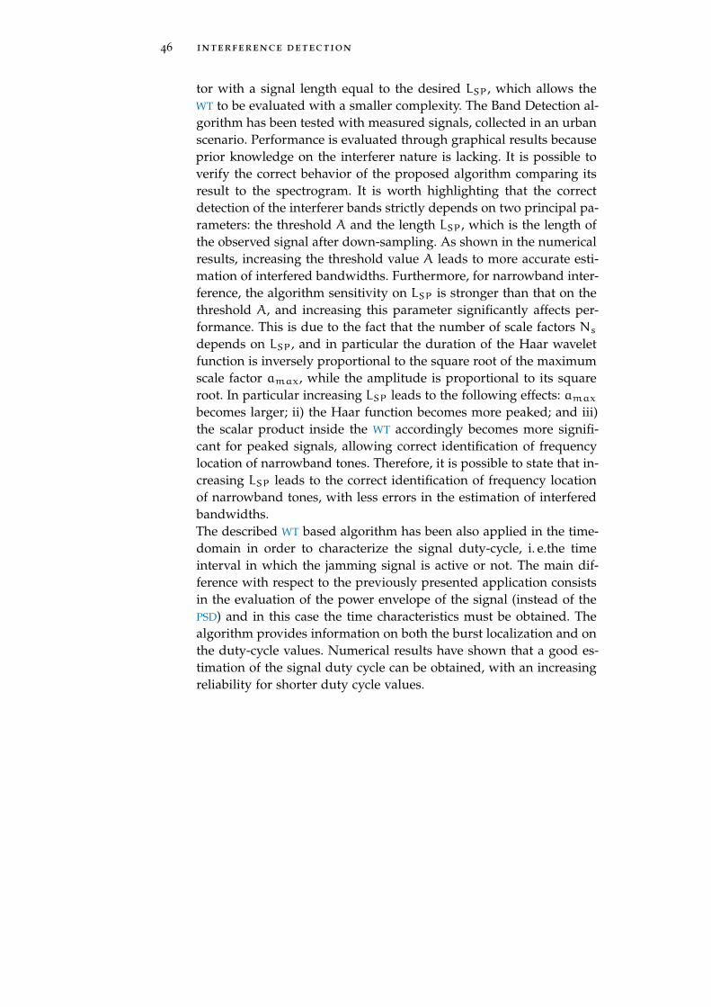
46 interference detection
tor with a signal length equal to the desired LSP, which allows theWT to be evaluated with a smaller complexity. The Band Detection al-gorithm has been tested with measured signals, collected in an urbanscenario. Performance is evaluated through graphical results becauseprior knowledge on the interferer nature is lacking. It is possible toverify the correct behavior of the proposed algorithm comparing itsresult to the spectrogram. It is worth highlighting that the correctdetection of the interferer bands strictly depends on two principal pa-rameters: the threshold A and the length LSP, which is the length ofthe observed signal after down-sampling. As shown in the numericalresults, increasing the threshold value A leads to more accurate esti-mation of interfered bandwidths. Furthermore, for narrowband inter-ference, the algorithm sensitivity on LSP is stronger than that on thethreshold A, and increasing this parameter significantly affects per-formance. This is due to the fact that the number of scale factors Nsdepends on LSP, and in particular the duration of the Haar waveletfunction is inversely proportional to the square root of the maximumscale factor amax, while the amplitude is proportional to its squareroot. In particular increasing LSP leads to the following effects: amaxbecomes larger; ii) the Haar function becomes more peaked; and iii)the scalar product inside the WT accordingly becomes more signifi-cant for peaked signals, allowing correct identification of frequencylocation of narrowband tones. Therefore, it is possible to state that in-creasing LSP leads to the correct identification of frequency locationof narrowband tones, with less errors in the estimation of interferedbandwidths.The described WT based algorithm has been also applied in the time-domain in order to characterize the signal duty-cycle, i. e.the timeinterval in which the jamming signal is active or not. The main dif-ference with respect to the previously presented application consistsin the evaluation of the power envelope of the signal (instead of thePSD) and in this case the time characteristics must be obtained. Thealgorithm provides information on both the burst localization and onthe duty-cycle values. Numerical results have shown that a good es-timation of the signal duty cycle can be obtained, with an increasingreliability for shorter duty cycle values.
2G N S S J A M M E R I N M U LT I PAT H S C E N A R I O
2.1 introduction
As explained previously in Chapter 1, the aim of GNSS jammers is todeny the correct reception of navigation signals, and as such they rep-resent one of the dominant threats to GNSS services and in particularof their availability. There is a clear necessity for techniques and al-gorithms to enhance the robustness to jammers in GNSS receivers, thebest option being the ability to isolate and cancel out the interferingsignal. Considering land mobile GNSS applications, usually the jam-mer will be located on the earth surface and direct visibility to the tar-get will only be sporadic, inasmuch as propagation will be enrichedby multiple reflection, diffraction, and absorption effects. Therefore,the interfering signal will typically reach the GNSS antenna through amultipath channel, possibly without a line-of-sight, and the receiverwill be faced with a number of malicious echoes generated by thechannel power delay profile, which render interference cancellation aphenomenal task. In this chapter, starting from the Interference Char-acterization and Cancellation (ICC) algorithm proposed in [P4][Pr1]and exhaustively described in [28], we present a solution to the prob-lem of cancelling GNSS jammer signals affected by multipath which isboth effective and computationally efficient. Specifically, we refer tointerfering attacks by means of personal devices, as evidenced in sev-eral measurement campaigns [30][48][12], which present a periodicand structured autocorrelation function. In the absence of multipath,this structure is static and can be exploited to estimate an effectiveinterference reference period upon which the ICC algorithm can beapplied. This is all very well, but assuming a non-frequency selec-tive channel is rather optimistic, as we clarified above. Moving fromthese results, the extension to the multipath scenario can be an in-teresting case. Exploring the literature on multipath effects on GNSSreceivers, it is immediate to observe that, while it is recognized thatmultipath is a critical issue in the development of high-performanceGNSS applications and reducing its adverse effects is a priority, theattention has been focused almost entirely on the consequent im-pact on desired GNSS signals and/or on PVT calculation[84][1][64][3].Extremely rare are those who considered the fragmentation of in-terference due to dispersed power delay profiles; in [2] space-timeadaptive processing techniques are used to mitigate the presence ofGNSS interference in a multipath environment. It could appear thatthe solution might entail a simple replication in parallel of the ICC
algorithm into a sufficient number of branches to match the popula-tion of significant multipath components. This is one case where sim-plicity of ideation is opposed to simplicity of implementation. Themain idea of this approach comes from recognizing that propaga-
47
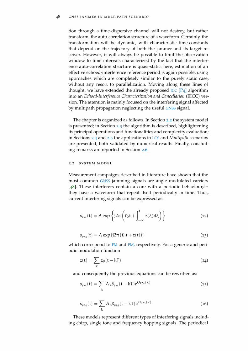
48 gnss jammer in multipath scenario
tion through a time-dispersive channel will not destroy, but rathertransform, the auto-correlation structure of a waveform. Certainly, thetransformation will be dynamic, with characteristic time-constantsthat depend on the trajectory of both the jammer and its target re-ceiver. However, it will always be possible to limit the observationwindow to time intervals characterized by the fact that the interfer-ence auto-correlation structure is quasi-static: here, estimation of aneffective echoed-interference reference period is again possible, usingapproaches which are completely similar to the purely static case,without any resort to parallelization. Moving along these lines ofthought, we have extended the already proposed ICC [P4] algorithminto an Echoed-Interference Characterization and Cancellation (EICC) ver-sion. The attention is mainly focused on the interfering signal affectedby multipath propagation neglecting the useful GNSS signal.
The chapter is organized as follows. In Section 2.2 the system modelis presented; in Section 2.3 the algorithm is described, highlighteningits principal operations and functionalities and complexity evaluation;in Sections 2.4 and 2.5 the applications in LOS and Multipath scenariosare presented, both validated by numerical results. Finally, conclud-ing remarks are reported in Section 2.6.
2.2 system model
Measurement campaigns described in literature have shown that themost common GNSS jamming signals are angle modulated carriers[48]. These interferers contain a core with a periodic behaviour,i.e.they have a waveform that repeat itself periodically in time. Thus,current interfering signals can be expressed as:
sFM
(t) = A exp{j2π
(f0t+
∫t−∞ z(ξ)dξ
)}(12)
sPM
(t) = A exp {j2π (f0t+ z(t))} (13)
which correspond to FM and PM, respectively. For a generic and peri-odic modulation function
z(t) =∑k
z0(t− kT) (14)
and consequently the previous equations can be rewritten as:
sFM
(t) =∑k
AksFM(t− kT)eΘFM(k) (15)
sPM
(t) =∑k
AksPM(t− kT)eΘPM(k) (16)
These models represent different types of interfering signals includ-ing chirp, single tone and frequency hopping signals. The periodical
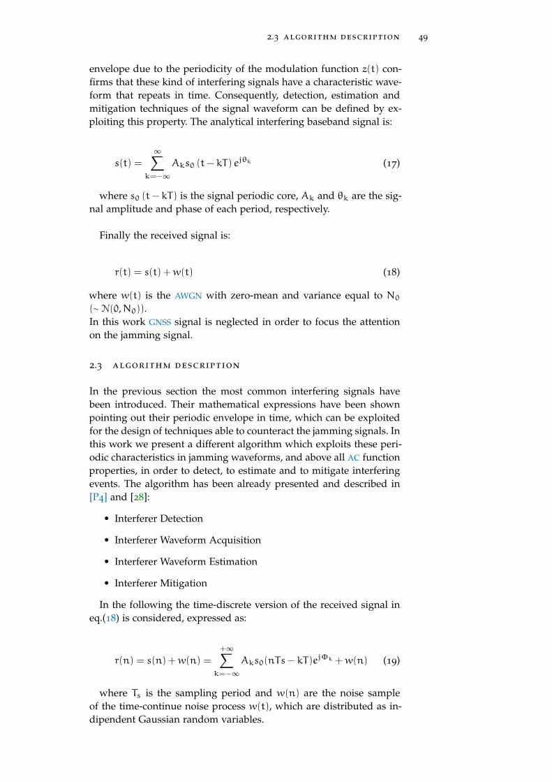
2.3 algorithm description 49
envelope due to the periodicity of the modulation function z(t) con-firms that these kind of interfering signals have a characteristic wave-form that repeats in time. Consequently, detection, estimation andmitigation techniques of the signal waveform can be defined by ex-ploiting this property. The analytical interfering baseband signal is:
s(t) =
∞∑k=−∞Aks0 (t− kT) e
jθk (17)
where s0 (t− kT) is the signal periodic core, Ak and θk are the sig-nal amplitude and phase of each period, respectively.
Finally the received signal is:
r(t) = s(t) +w(t) (18)
where w(t) is the AWGN with zero-mean and variance equal to N0(∼ N(0,N0)).In this work GNSS signal is neglected in order to focus the attentionon the jamming signal.
2.3 algorithm description
In the previous section the most common interfering signals havebeen introduced. Their mathematical expressions have been shownpointing out their periodic envelope in time, which can be exploitedfor the design of techniques able to counteract the jamming signals. Inthis work we present a different algorithm which exploits these peri-odic characteristics in jamming waveforms, and above all AC functionproperties, in order to detect, to estimate and to mitigate interferingevents. The algorithm has been already presented and described in[P4] and [28]:
• Interferer Detection
• Interferer Waveform Acquisition
• Interferer Waveform Estimation
• Interferer Mitigation
In the following the time-discrete version of the received signal ineq.(18) is considered, expressed as:
r(n) = s(n) +w(n) =
+∞∑k=−∞Aks0(nTs− kT)e
jΦk +w(n) (19)
where Ts is the sampling period and w(n) are the noise sampleof the time-continue noise process w(t), which are distributed as in-dipendent Gaussian random variables.
50 gnss jammer in multipath scenario
2.3.1 Interferer Detection
The Detection consists in observing the received signal in order tofind any interfering event that may occour. The detection procedureis based on the AC function of the received signal. If a structured inter-fering signal is present, the AC function presents several peaks in theconsidered time window. These peaks correspond to the repetitionperiod T . Thus, it is possible to design a simple way in jamming de-tection by exploiting this periodic characteristic. Detection procedurepresents three steps:
1. The AC function is evaluated according to the Wiener-Kintchinetheorem by means of the Fourier Transform (FT) and then nor-malized in order to have unit power (at zero-lag).
2. The detection test variable is evaluated as the maximum asbso-lute value of the AC function neglecting the zero-lag sample inorder to find the next maximum value.
3. The test is compared against a set threshold ξ.
It is worthwhile to notice that due to the finite observation time, theAC function can be estimated, thus no true value can be carried out.The procedure is described also in Algorithm 4 and shown in Figure(61).
Interference Detection Algorithm
1) Rrr∗(m) = F−1{F {r(n)} ·F {r(n)}∗
};
Rrr(m) =Rrr∗(m)Rrr∗(0)
;
2) Test = max |Rrr∗(m)| m 6= 0 ;
3) Test ≷ ξ ;
Algorithmus 4 : Interference Detection Algorithm
Figure 61: Interferer Detection - Block Diagram.
In the first step the circular correlation is performed by the Dis-crete Fourier Transform (DFT) where F {} and F−1 {} are the DFT andthe inverse DFT, respectively. These operations can be calculated bythe efficient numerical tools FFT and Inverse FFT (IFFT) for a large val-ues of N, which is the signal samples in the observation windows.The AC function Rrr∗(m) is defined for m ∈ [Mmin,Mmax], i. e.fora limited number of lags. This interval has to be defined in order tobe able to detect all the possible structured interferers, which couldhave different periods. Thus, it is necessary to properly define theseparameters with the aim of detecting different jamming signal withdifferent repetition period T .
2.3 algorithm description 51
2.3.1.1 Statistical Parameter Setting
Taking into account the Algorithm 4, it is necessary to set the lag-interval in which the AC function has to be evaluated. In [12] and[48] the measurement campaigns have highlightened that jammingsignals have repetition periods varying usually from 1µs to 50µs withsome longer exceptions (∼ 70µs). As stated before, the number oflags has to be larger enough in order to detect at least one repetitionperiod, and so we have:
MmaxTs > T (20)
The detection problem is defined as a binary decision problem,with two hypotheses:
• H1 : the Test is greater than the threshold. The jammer is de-tected and the AC function peaks are located at each repetitionperiod instant
• H0 : the Test is lower than the threshold, meaning that any peakis present.
The AC function at the step 1 of the algorithm is defined by meansof the product of FT transforms and it can be assumed as the resultsof average sum of products of the received signal samples, whichare considered statistically indipendent each others. Neglecting theenergy at the zero-lag (m 6= 0), at each repetition period the cor-responding AC peak has energy equal to the average signal energy.The received signal r(n) expressed in eq.(19) can be statistically ex-pressed as a Gaussian random variable with mean equal to µr = A
and variance σ2r = N0, due to the deterministic nature of s(n) andw(n) ∼ N(0,N0). Considering that the evaluation of the mean andvariance of a random variable defined as the product of two indipen-dent variables (a and b) are, respectively:
E[ab] = E[a]E[b] (21)
Var(ab) = E2[a]Var(b) + E2[b]Var(a) + Var(a)Var(b)
it is possible to define the statistical values of the single signal prod-uct as:
µrr∗ = A2 (22)
σ2rr∗ = σ2r(2µrr + σ
2r
)(23)
where the amplitude A is considered constant in each time periodrepetition. Consequently it is possible to define the statistical proper-ties of the AC function, which can be expressed as:
52 gnss jammer in multipath scenario
µR =A2
A2 + σ2r=
A2
σ2r
1+ A2
σ2r
(24)
σ2R =1
M
σrr∗
(A2 + σ2r)2=1
M
1+ 2A2
σ2r(1+ A2
σ2r
)2 (25)
due to the Jammer-to-Noise Ratio (JNR) A2
σ2rand lags (M) normaliza-
tion. Once statistical values of the AC have been defined, it is possibleto evaluate the power value at the peak of the AC function as:
JNRAC =µ2Rσ2R
(26)
= M
A4
σ4r(1+ A2
σ2r
)2= M
JNR2
1+ 2JNR
At the same way, it is necessary to evaluate statistical propertiesfor the hypothesis H0, i. e.when the interfering signal is not present.Thus, it is possible to express with the same procedure as above themean and variance values of the product of received signal samples:
µrr∗ = 0 (27)
σrr∗ = σ4r (28)
and the corresponding statistical properties for AC function underH0 are:
µR = 0 (29)
σR =1
M(30)
JNRAC = 0 (31)
2.3.1.2 Detector Design
As previously stated, the detection of the interfering signal is mod-eled as a binary decision problem with two hypotheses H1 the in-terfering signal is present, H0 the interfering signal is absent. Thedecision test has been defined as the maximum of the absolute valueof the AC function of the received signal, as described at the step 2 ofthe algorithm 4. The AC function has been evaluated by averaging alarge number of products between random variables, thus it is possi-ble to define the AC function Gaussian distributed random variable.
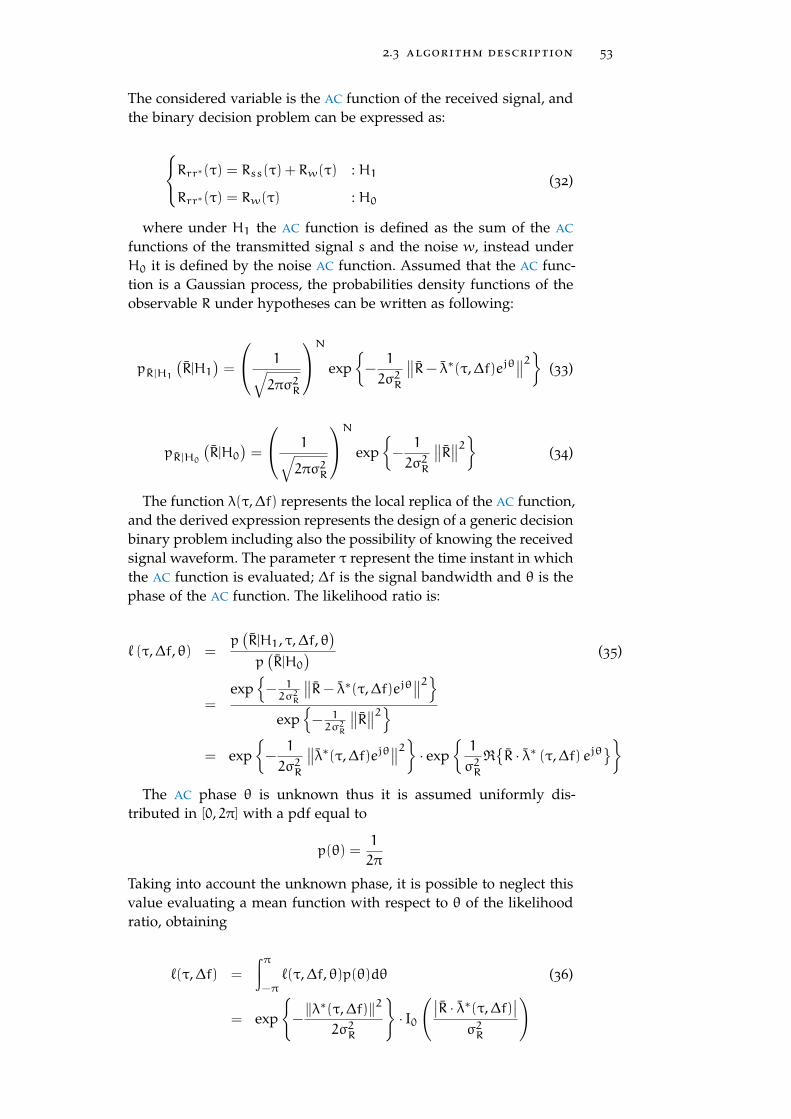
2.3 algorithm description 53
The considered variable is the AC function of the received signal, andthe binary decision problem can be expressed as:
Rrr∗(τ) = Rss(τ) + Rw(τ) : H1
Rrr∗(τ) = Rw(τ) : H0
(32)
where under H1 the AC function is defined as the sum of the AC
functions of the transmitted signal s and the noise w, instead underH0 it is defined by the noise AC function. Assumed that the AC func-tion is a Gaussian process, the probabilities density functions of theobservable R under hypotheses can be written as following:
pR|H1
(R|H1
)=
1√2πσ2R
N exp{−1
2σ2R
∥∥R− λ∗(τ,∆f)ejθ∥∥2} (33)
pR|H0
(R|H0
)=
1√2πσ2R
N exp{−1
2σ2R
∥∥R∥∥2} (34)
The function λ(τ,∆f) represents the local replica of the AC function,and the derived expression represents the design of a generic decisionbinary problem including also the possibility of knowing the receivedsignal waveform. The parameter τ represent the time instant in whichthe AC function is evaluated; ∆f is the signal bandwidth and θ is thephase of the AC function. The likelihood ratio is:
` (τ,∆f, θ) =p(R|H1, τ,∆f, θ
)p(R|H0
) (35)
=exp{− 12σ2R
∥∥R− λ∗(τ,∆f)ejθ∥∥2}
exp{− 12σ2R
∥∥R∥∥2}= exp
{−1
2σ2R
∥∥λ∗(τ,∆f)ejθ∥∥2} · exp
{1
σ2R<{R · λ∗ (τ,∆f) ejθ
}}The AC phase θ is unknown thus it is assumed uniformly dis-
tributed in [0, 2π] with a pdf equal to
p(θ) =1
2π
Taking into account the unknown phase, it is possible to neglect thisvalue evaluating a mean function with respect to θ of the likelihoodratio, obtaining
`(τ,∆f) =
∫π−π`(τ,∆f, θ)p(θ)dθ (36)
= exp
{−‖λ∗(τ,∆f)‖2
2σ2R
}· I0
(∣∣R · λ∗(τ,∆f)∣∣
σ2R
)
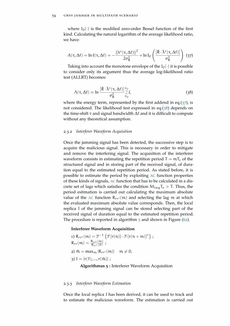
54 gnss jammer in multipath scenario
where I0(·) is the modified zero-order Bessel function of the firstkind. Calculating the natural logarithm of the average likelihood ratio,we have:
Λ(τ,∆f) = ln `(τ,∆f) = −‖λ∗(τ,∆f)‖2
2σ2R+ ln I0
(∣∣R · λ∗(τ,∆f)∣∣
σ2R
)(37)
Taking into account the monotone envelope of the I0(·) it is possibleto consider only its argument thus the average log-likelihood ratiotest (ALLRT) becomes:
Λ(τ,∆f) ' ln
∣∣R · λ∗(τ,∆f)∣∣
σ2R
H1><H0
ξ (38)
where the energy term, represented by the first addend in eq.(37), isnot considered. The likelihood test expressed in eq.(38) depends onthe time-shift τ and signal bandwidth ∆f and it is difficult to computewithout any theoretical assumption.
2.3.2 Interferer Waveform Acquisition
Once the jamming signal has been detected, the successive step is toacquire the malicious signal. This is necessary in order to mitigateand remove the interfering signal. The acquisition of the interfererwaveform consists in estimating the repetition period T = mTs of thestructured signal and in storing part of the received signal, of dura-tion equal to the estimated repetition period. As stated before, it ispossible to estimate the period by exploiting AC function propertiesof these kinds of signals, AC function that has to be calculated in a dis-crete set of lags which satisfies the condition MlagTs > T . Thus, theperiod estimation is carried out calculating the maximum absolutevalue of the AC function Rrr∗(m) and selecting the lag m at whichthe evaluated maximum absolute value corresponds. Then, the localreplica I of the jamming signal can be stored selecting part of thereceived signal of duration equal to the estimated repetition period.The procedure is reported in algorithm 5 and shown in Figure (62).
Interferer Waveform Acquisition
1) Rrr∗(m) = F−1{F {r(n)} ·F {r(n+m)}∗
};
Rrr(m) =Rrr∗(m)Rrr∗(0)
;
2) m = maxm |Rrr∗(m)| m 6= 0;
3) I = [r(1), ..., r(m)] ;
Algorithmus 5 : Interferer Waveform Acquisition
2.3.3 Interferer Waveform Estimation
Once the local replica I has been derived, it can be used to track andto estimate the malicious waveform. The estimation is carried out
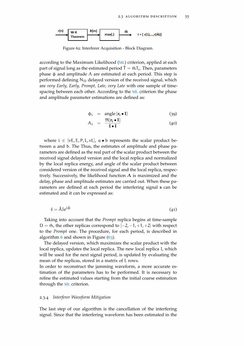
2.3 algorithm description 55
Figure 62: Interferer Acquisition - Block Diagram.
according to the Maximum Likelihood (ML) criterion, applied at eachpart of signal long as the estimated period T = mTs. Then, parametersphase φ and amplitude A are estimated at each period. This step isperformed defining ND delayed version of the received signal, whichare very Early, Early, Prompt, Late, very Late with one sample of time-spacing between each other. According to the ML criterion the phaseand amplitude parameter estimations are defined as:
φi = angle {ri • I} (39)
Ai =<{ri • I}
I • I(40)
where i ∈ [vE,E,P,L, vL], a • b represents the scalar product be-tween a and b. The Thus, the estimates of amplitude and phase pa-rameters are defined as the real part of the scalar product between thereceived signal delayed version and the local replica and normalizedby the local replica energy, and angle of the scalar product betweenconsidered version of the received signal and the local replica, respec-tively. Successively, the likelihood function Λ is maximized and thedelay, phase and amplitude estimates are carried out. When these pa-rameters are defined at each period the interfering signal s can beestimated and it can be expressed as:
s = AIejφ (41)
Taking into account that the Prompt replica begins at time-sampleD = m, the other replicas correspond to [−2,−1,+1,+2] with respectto the Prompt one. The procedure, for each period, is described inalgorithm 6 and shown in Figure (63).
The delayed version, which maximizes the scalar product with thelocal replica, updates the local replica. The new local replica I, whichwill be used for the next signal period, is updated by evaluating themean of the replicas, stored in a matrix of L rows.In order to reconstruct the jamming waveform, a more accurate es-timation of the parameters has to be performed. It is necessary torefine the estimated values starting from the initial coarse estimationthrough the ML criterion.
2.3.4 Interferer Waveform Mitigation
The last step of our algorithm is the cancellation of the interferingsignal. Since that the interfering waveform has been estimated in the
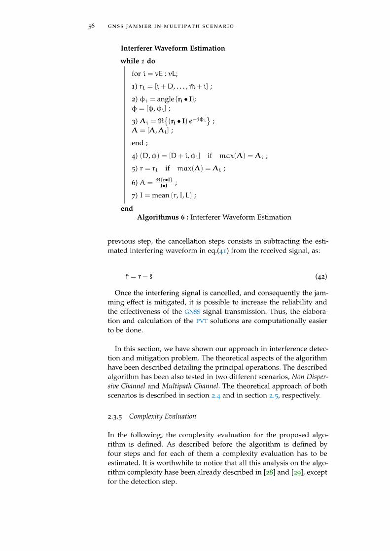
56 gnss jammer in multipath scenario
Interferer Waveform Estimation
while 1 do
for i = vE : vL;
1) ri = [i+D, . . . , m+ i] ;
2) φi = angle {ri • I};φ = [φ,φi] ;
3) Λi = <{(ri • I) e−jφi
};
Λ = [Λ,Λi] ;
end ;
4) (D,φ) = [D+ i,φi] if max(Λ) = Λi ;
5) r = ri if max(Λ) = Λi ;
6) A = <{r•I}I•I ;
7) I = mean (r, I,L) ;
endAlgorithmus 6 : Interferer Waveform Estimation
previous step, the cancellation steps consists in subtracting the esti-mated interfering waveform in eq.(41) from the received signal, as:
r = r− s (42)
Once the interfering signal is cancelled, and consequently the jam-ming effect is mitigated, it is possible to increase the reliability andthe effectiveness of the GNSS signal transmission. Thus, the elabora-tion and calculation of the PVT solutions are computationally easierto be done.
In this section, we have shown our approach in interference detec-tion and mitigation problem. The theoretical aspects of the algorithmhave been described detailing the principal operations. The describedalgorithm has been also tested in two different scenarios, Non Disper-sive Channel and Multipath Channel. The theoretical approach of bothscenarios is described in section 2.4 and in section 2.5, respectively.
2.3.5 Complexity Evaluation
In the following, the complexity evaluation for the proposed algo-rithm is defined. As described before the algorithm is defined byfour steps and for each of them a complexity evaluation has to beestimated. It is worthwhile to notice that all this analysis on the algo-rithm complexity hase been already described in [28] and [29], exceptfor the detection step.
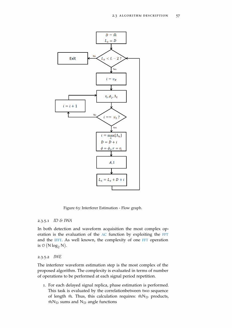
2.3 algorithm description 57
Figure 63: Interferer Estimation - Flow graph.
2.3.5.1 ID & IWA
In both detection and waveform acquisition the most complex op-eration is the evaluation of the AC function by exploiting the FFT
and the IFFT. As well known, the complexity of one FFT operationis O
(N log2N
).
2.3.5.2 IWE
The interferer waveform estimation step is the most complex of theproposed algorithm. The complexity is evaluated in terms of numberof operations to be performed at each signal period repetition.
1. For each delayed signal replica, phase estimation is performed.This task is evaluated by the correlationbetween two sequenceof length m. Thus, this calculation requires: mND products,mND sums and ND angle functions
58 gnss jammer in multipath scenario
2. Likelihood function Λ: delayed replicas are de-rotated by prod-ucts with the conjugate phase. evaluated before. Thus, ND com-plex products are implemented.
3. Amplitude estimation is performed as a the real part of the cor-relation between the delayed version which satisfies the maxi-mum Λ and the normalization by the local replica energy. Thus,only two products are implemented.
4. Updating of the Local replica I: the last step is to update thelocal replica. It is necessary to average L sequences of length m,requiring mL sums and L products.
2.3.5.3 IWM
The last step is the cancellation of the estimated jamming signal. Thispart consists in the difference between the received signal and thereconstructed interfering waveform. Thus, a simple difference is per-formed.
Finally, the total computational complexity of the algorithm canbe estimated. The proposed procedure needs a number of sums andproducts equal to:
Nsums = m (ND + 1+ L) (43)
Nprod = m (ND + 1+ 1) (44)
which highlight that the complexity is proportional to the lag m,which defines the estimated repetition period.
2.4 non-dispersive channel
Due to the increasing widespread of GNSS applications in human lifeactivities, it is necessary to define techniques able to counteract themalicious events that wants to deny the correct operation of the GNSS
receiver. As explained previously, the jamming threat in GNSS systemis a very hot topic and several research studies have been done. Mostof these results regard to detection and mitigation of the interferingevent in a non dispersive channel scenario. The jammer is in earthsurface and direct visibility to the target, thus the received signal isdefined as the jamming signal embedded in noise process, assumedto be a additive gaussian statistical process. In [29] an algorithm ableto cope with all the interfering signals with a structured envelope, isproposed. As extensively described in [28], the algorithm consists offour stages: i) waveform acquisition, ii) waveform tracking, iii) effec-tive interference parameter estimation, iv) interference cancellation.The performance is evaluated in terms of residual of cancellation andit has been carried out for three different types of signal, continuouswaveform, chirp and CDMA.
2.4 non-dispersive channel 59
2.4.1 Jamming Chirp
In our study we consider a jamming chirp signal. Chirp signals aredefined as FM signals in which the frequency increases or decreaseswith time, called "up-chirp" and "down-chirp", respectively. They arealso called as sweep signals. The modulation function can be classi-fied in two main categories, linear chirp modulation and exponentialchirp modulation, i. e.the swept in frequency is defined by a linearfunction or an exponential one, respectively. In the following, a chirpsignal with a frequency varying linearly in time is considered. Thejamming signal is expressed as:
s(t) = ArectT (t) cos(2π
∫t0
f(r)dr
)=
= ArectT (t) cos(2π
∫t0
[f0 ±
ρ
2πr]dr
)= ArectT (t) cos
(2πf0t± ρ
t2
2
)(45)
where ρ = 2π∆fT is the frequency variation rate, T is the pulse pe-
riod, f0 is the carrier frequency and ∆f is the frequency excursionduring a pulse period.
Taking into account eq.(17) and considering one signal period, thejamming basic waveform is:
s0(t) = exp{±jρt
2
2
}rect
(t
T
)(46)
In the following, an "up-chirp", with a positive frequency slope, isconsidered.
2.4.2 Jamming Chirp Autocorrelation Analysis
As highlighted in the previous section, the most common jammingsignals are structured and present a periodic envelope. Among them,one of the interesting case-study is represented by the chirp signal,which expression is shown in eq.(46). In order to exploit this periodiccharacteristics, a complete analysis of the AC function is carried out.The spectrum of the chirp signal is evaluated through the FT of thesignal which is expressed as:
S(f) =
∫+∞−∞ s(t)e−j2πftdt (47)
=
∫T/2−T/2
ejρ2 t2
e−j2πftdt
=
∫T/2−T/2
ej(ρ2 t2−2πft)dt
60 gnss jammer in multipath scenario
The argument of the exponential function can be considered as thesquare of a difference without the square of the second term. Thus,we have:
ρ
2t2 − 2πft = (a− b)2 − b2 (48)
= a2 − 2ab
From eq.(48) it is possible to define a =√ρ2 t and b = πf
√2ρ and
so the exponent in eq.(47) can be written as:
ρ
2t2 − 2πft =
(√ρ
2t− πf
√2
ρ
)2−2
ρ(πf)2 (49)
Thus, the chirp spectrum expression is:
S(f) = e−j2(πf)2
ρ
∫T/2−T/2
ej(√
ρ2 t−πf
√2ρ
)2dt (50)
=
√π
ρe−j
2(πf)2
ρ
∫Z2Z1
ejπy2
2 dy
The last expression is obtained through the substitution√ρ
2t− πf
√2
ρ=
√π
2y
and the derivation of the corresponding integration interval
Z1 =
√ρ
πT
(−1
2−f
∆f
)=√2∆fT
(−1
2−f
∆f
)=√2∆fT
(−∆f− 2f
2∆f
)(51)
Z2 =
√ρ
πT
(1
2−f
∆f
)=√2∆fT
(1
2−f
∆f
)=√2∆fT
(∆f− 2f
2∆f
)(52)
The last expression of the chirp spectrum can be considered asa linear combination of Fresnel integral functions. It is possible tonotice that the expression of eq.(50) is the Fresnel integral E(x) =
C(x) + jS(x), where
C(x) =
∫x0
cos(πy2
2
)dy
S(x) =
∫x0
sin(πy2
2
)dy
Finally, the chirp spectrum can be expressed as:
S(f) =
√π
ρe−j
2(πf)2
ρ {C(Z2) +C(−Z1) + j [S(Z2) + S(−Z1)]}
=
√π
ρe−j
2(πf)2
ρ {E(Z2) + E(−Z1)} (53)
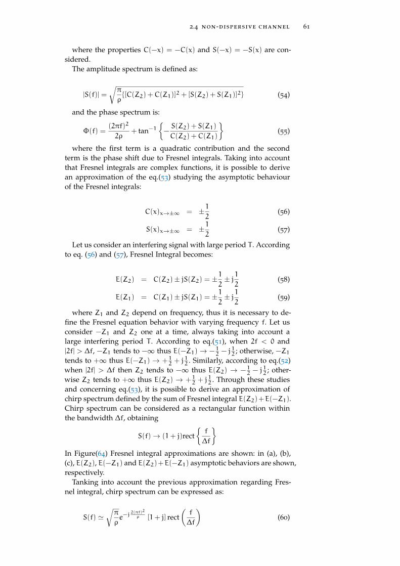
2.4 non-dispersive channel 61
where the properties C(−x) = −C(x) and S(−x) = −S(x) are con-sidered.
The amplitude spectrum is defined as:
|S(f)| =
√π
ρ{[C(Z2) +C(Z1)]2 + [S(Z2) + S(Z1)]2} (54)
and the phase spectrum is:
Φ(f) =(2πf)2
2ρ+ tan−1
{−S(Z2) + S(Z1)
C(Z2) +C(Z1)
}(55)
where the first term is a quadratic contribution and the secondterm is the phase shift due to Fresnel integrals. Taking into accountthat Fresnel integrals are complex functions, it is possible to derivean approximation of the eq.(53) studying the asymptotic behaviourof the Fresnel integrals:
C(x)x→±∞ = ±12
(56)
S(x)x→±∞ = ±12
(57)
Let us consider an interfering signal with large period T . Accordingto eq. (56) and (57), Fresnel Integral becomes:
E(Z2) = C(Z2)± jS(Z2) = ±1
2± j12
(58)
E(Z1) = C(Z1)± jS(Z1) = ±1
2± j12
(59)
where Z1 and Z2 depend on frequency, thus it is necessary to de-fine the Fresnel equation behavior with varying frequency f. Let usconsider −Z1 and Z2 one at a time, always taking into account alarge interfering period T . According to eq.(51), when 2f < 0 and|2f| > ∆f, −Z1 tends to −∞ thus E(−Z1)→ −12 − j
12 ; otherwise, −Z1
tends to +∞ thus E(−Z1) → +12 + j12 . Similarly, according to eq.(52)
when |2f| > ∆f then Z2 tends to −∞ thus E(Z2) → −12 − j12 ; other-
wise Z2 tends to +∞ thus E(Z2) → +12 + j12 . Through these studies
and concerning eq.(53), it is possible to derive an approximation ofchirp spectrum defined by the sum of Fresnel integral E(Z2)+E(−Z1).Chirp spectrum can be considered as a rectangular function withinthe bandwidth ∆f, obtaining
S(f)→ (1+ j)rect{f
∆f
}In Figure(64) Fresnel integral approximations are shown: in (a), (b),(c), E(Z2), E(−Z1) and E(Z2)+E(−Z1) asymptotic behaviors are shown,respectively.
Tanking into account the previous approximation regarding Fres-nel integral, chirp spectrum can be expressed as:
S(f) '√π
ρe−j
2(πf)2
ρ [1+ j] rect(f
∆f
)(60)
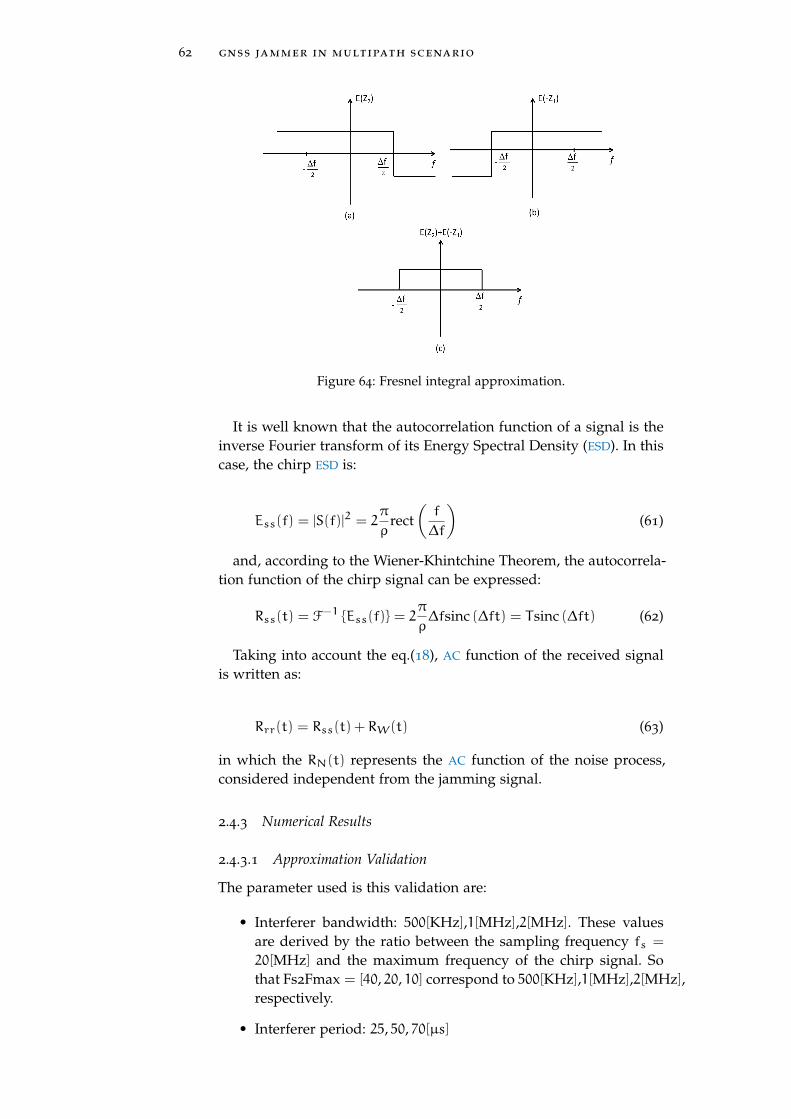
62 gnss jammer in multipath scenario
Figure 64: Fresnel integral approximation.
It is well known that the autocorrelation function of a signal is theinverse Fourier transform of its Energy Spectral Density (ESD). In thiscase, the chirp ESD is:
Ess(f) = |S(f)|2 = 2π
ρrect
(f
∆f
)(61)
and, according to the Wiener-Khintchine Theorem, the autocorrela-tion function of the chirp signal can be expressed:
Rss(t) = F−1 {Ess(f)} = 2π
ρ∆fsinc (∆ft) = Tsinc (∆ft) (62)
Taking into account the eq.(18), AC function of the received signalis written as:
Rrr(t) = Rss(t) + RW(t) (63)
in which the RN(t) represents the AC function of the noise process,considered independent from the jamming signal.
2.4.3 Numerical Results
2.4.3.1 Approximation Validation
The parameter used is this validation are:
• Interferer bandwidth: 500[KHz],1[MHz],2[MHz]. These valuesare derived by the ratio between the sampling frequency fs =
20[MHz] and the maximum frequency of the chirp signal. Sothat Fs2Fmax = [40, 20, 10] correspond to 500[KHz],1[MHz],2[MHz],respectively.
• Interferer period: 25, 50, 70[µs]
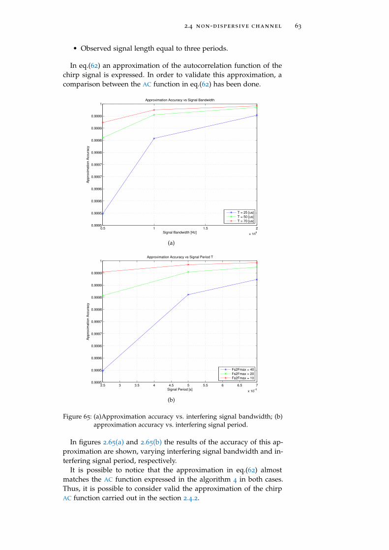
2.4 non-dispersive channel 63
• Observed signal length equal to three periods.
In eq.(62) an approximation of the autocorrelation function of thechirp signal is expressed. In order to validate this approximation, acomparison between the AC function in eq.(62) has been done.
0.5 1 1.5 2
x 106
0.9995
0.9995
0.9996
0.9996
0.9997
0.9997
0.9998
0.9998
0.9999
0.9999
1
Signal Bandwidth [Hz]
Ap
pro
xim
atio
n A
ccu
racy
Approximation Accuracy vs Signal Bandwidth
T = 25 [us]
T = 50 [us]
T = 70 [us]
(a)
2.5 3 3.5 4 4.5 5 5.5 6 6.5 7
x 10−5
0.9995
0.9995
0.9996
0.9996
0.9997
0.9997
0.9998
0.9998
0.9999
0.9999
1
Signal Period [s]
Ap
pro
xim
atio
n A
ccu
racy
Approximation Accuracy vs Signal Period T
Fs2Fmax = 40
Fs2Fmax = 20
Fs2Fmax = 10
(b)
Figure 65: (a)Approximation accuracy vs. interfering signal bandwidth; (b)approximation accuracy vs. interfering signal period.
In figures 2.65(a) and 2.65(b) the results of the accuracy of this ap-proximation are shown, varying interfering signal bandwidth and in-terfering signal period, respectively.
It is possible to notice that the approximation in eq.(62) almostmatches the AC function expressed in the algorithm 4 in both cases.Thus, it is possible to consider valid the approximation of the chirpAC function carried out in the section 2.4.2.
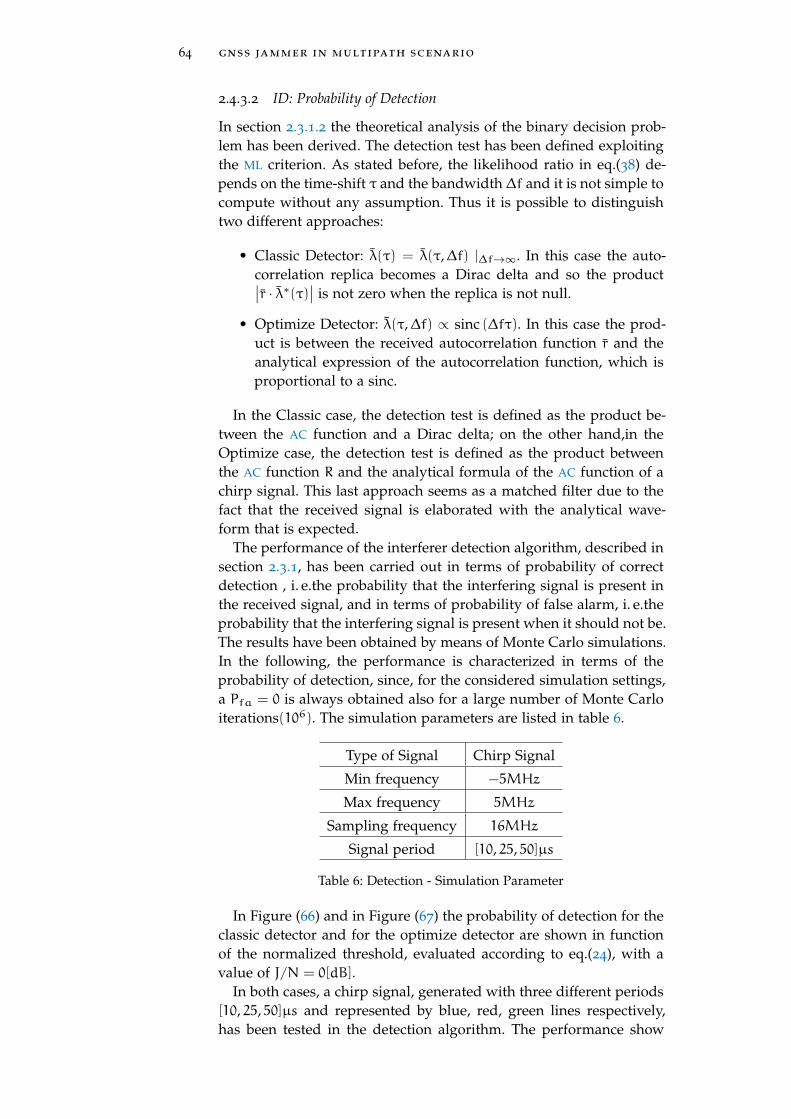
64 gnss jammer in multipath scenario
2.4.3.2 ID: Probability of Detection
In section 2.3.1.2 the theoretical analysis of the binary decision prob-lem has been derived. The detection test has been defined exploitingthe ML criterion. As stated before, the likelihood ratio in eq.(38) de-pends on the time-shift τ and the bandwidth ∆f and it is not simple tocompute without any assumption. Thus it is possible to distinguishtwo different approaches:
• Classic Detector: λ(τ) = λ(τ,∆f) |∆f→∞. In this case the auto-correlation replica becomes a Dirac delta and so the product∣∣r · λ∗(τ)∣∣ is not zero when the replica is not null.
• Optimize Detector: λ(τ,∆f) ∝ sinc (∆fτ). In this case the prod-uct is between the received autocorrelation function r and theanalytical expression of the autocorrelation function, which isproportional to a sinc.
In the Classic case, the detection test is defined as the product be-tween the AC function and a Dirac delta; on the other hand,in theOptimize case, the detection test is defined as the product betweenthe AC function R and the analytical formula of the AC function of achirp signal. This last approach seems as a matched filter due to thefact that the received signal is elaborated with the analytical wave-form that is expected.
The performance of the interferer detection algorithm, described insection 2.3.1, has been carried out in terms of probability of correctdetection , i. e.the probability that the interfering signal is present inthe received signal, and in terms of probability of false alarm, i. e.theprobability that the interfering signal is present when it should not be.The results have been obtained by means of Monte Carlo simulations.In the following, the performance is characterized in terms of theprobability of detection, since, for the considered simulation settings,a Pfa = 0 is always obtained also for a large number of Monte Carloiterations(106). The simulation parameters are listed in table 6.
Type of Signal Chirp Signal
Min frequency −5MHz
Max frequency 5MHz
Sampling frequency 16MHz
Signal period [10, 25, 50]µs
Table 6: Detection - Simulation Parameter
In Figure (66) and in Figure (67) the probability of detection for theclassic detector and for the optimize detector are shown in functionof the normalized threshold, evaluated according to eq.(24), with avalue of J/N = 0[dB].
In both cases, a chirp signal, generated with three different periods[10, 25, 50]µs and represented by blue, red, green lines respectively,has been tested in the detection algorithm. The performance show
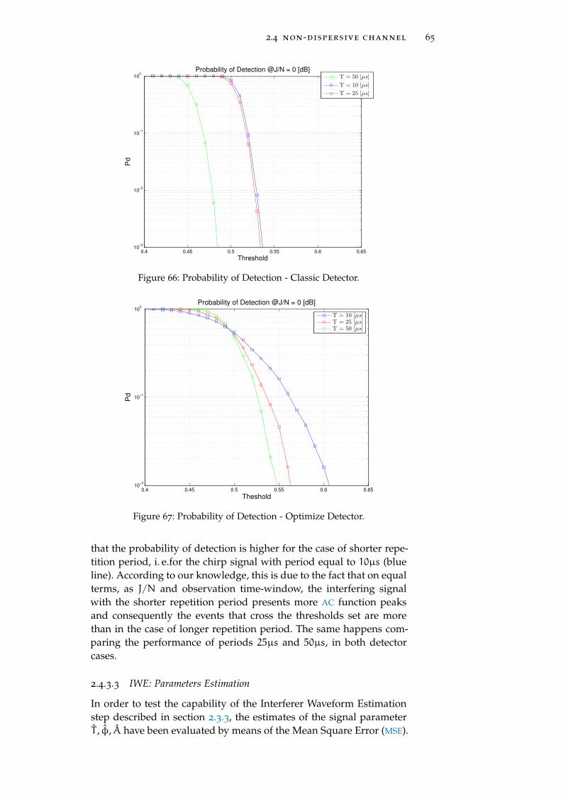
2.4 non-dispersive channel 65
0.4 0.45 0.5 0.55 0.6 0.6510
−3
10−2
10−1
100
Threshold
Pd
Probability of Detection @J/N = 0 [dB]
T = 50 [µs]
T = 10 [µs]
T = 25 [µs]
Figure 66: Probability of Detection - Classic Detector.
0.4 0.45 0.5 0.55 0.6 0.6510
−2
10−1
100
Theshold
Pd
Probability of Detection @J/N = 0 [dB]
T = 10 [µs]T = 25 [µs]T = 50 [µs]
Figure 67: Probability of Detection - Optimize Detector.
that the probability of detection is higher for the case of shorter repe-tition period, i. e.for the chirp signal with period equal to 10µs (blueline). According to our knowledge, this is due to the fact that on equalterms, as J/N and observation time-window, the interfering signalwith the shorter repetition period presents more AC function peaksand consequently the events that cross the thresholds set are morethan in the case of longer repetition period. The same happens com-paring the performance of periods 25µs and 50µs, in both detectorcases.
2.4.3.3 IWE: Parameters Estimation
In order to test the capability of the Interferer Waveform Estimationstep described in section 2.3.3, the estimates of the signal parameterT , φ, A have been evaluated by means of the Mean Square Error (MSE).
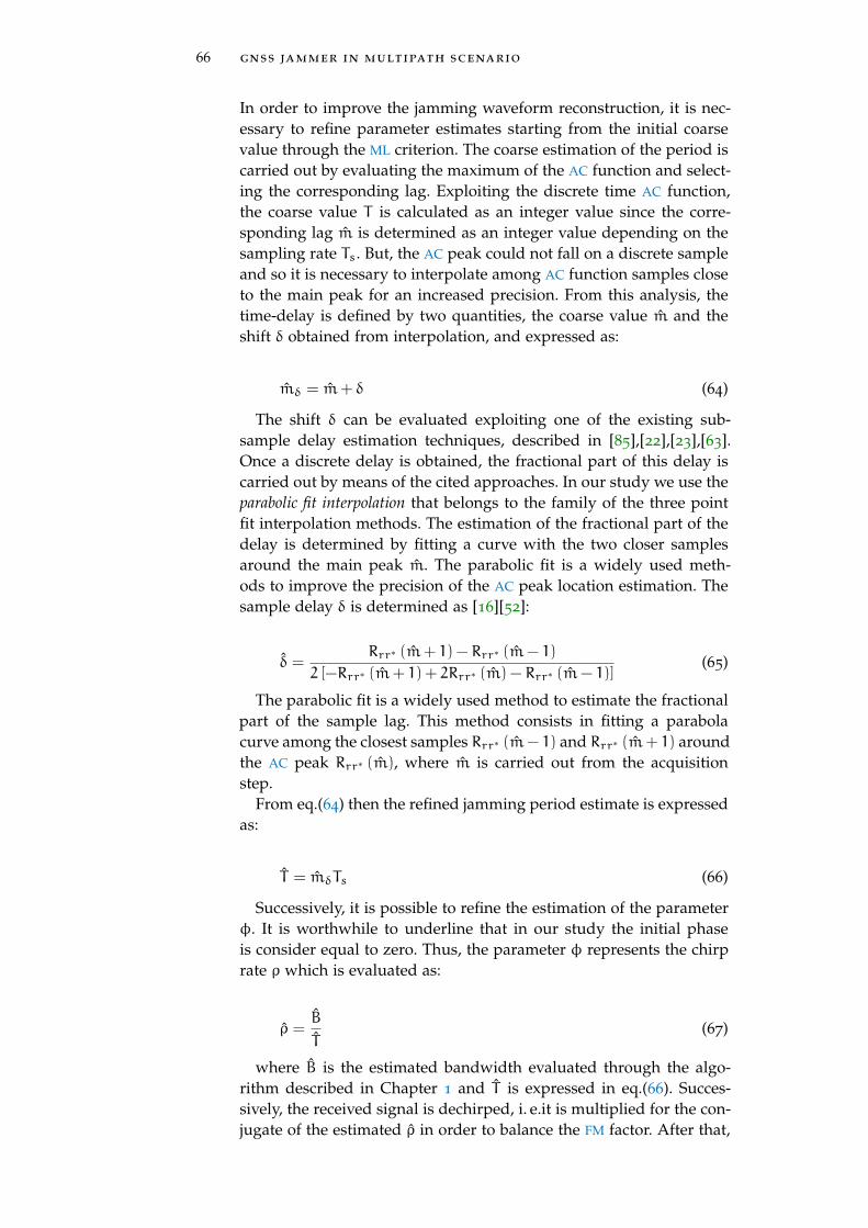
66 gnss jammer in multipath scenario
In order to improve the jamming waveform reconstruction, it is nec-essary to refine parameter estimates starting from the initial coarsevalue through the ML criterion. The coarse estimation of the period iscarried out by evaluating the maximum of the AC function and select-ing the corresponding lag. Exploiting the discrete time AC function,the coarse value T is calculated as an integer value since the corre-sponding lag m is determined as an integer value depending on thesampling rate Ts. But, the AC peak could not fall on a discrete sampleand so it is necessary to interpolate among AC function samples closeto the main peak for an increased precision. From this analysis, thetime-delay is defined by two quantities, the coarse value m and theshift δ obtained from interpolation, and expressed as:
mδ = m+ δ (64)
The shift δ can be evaluated exploiting one of the existing sub-sample delay estimation techniques, described in [85],[22],[23],[63].Once a discrete delay is obtained, the fractional part of this delay iscarried out by means of the cited approaches. In our study we use theparabolic fit interpolation that belongs to the family of the three pointfit interpolation methods. The estimation of the fractional part of thedelay is determined by fitting a curve with the two closer samplesaround the main peak m. The parabolic fit is a widely used meth-ods to improve the precision of the AC peak location estimation. Thesample delay δ is determined as [16][52]:
δ =Rrr∗ (m+ 1) − Rrr∗ (m− 1)
2 [−Rrr∗ (m+ 1) + 2Rrr∗ (m) − Rrr∗ (m− 1)](65)
The parabolic fit is a widely used method to estimate the fractionalpart of the sample lag. This method consists in fitting a parabolacurve among the closest samples Rrr∗ (m− 1) and Rrr∗ (m+ 1) aroundthe AC peak Rrr∗ (m), where m is carried out from the acquisitionstep.
From eq.(64) then the refined jamming period estimate is expressedas:
T = mδTs (66)
Successively, it is possible to refine the estimation of the parameterφ. It is worthwhile to underline that in our study the initial phaseis consider equal to zero. Thus, the parameter φ represents the chirprate ρ which is evaluated as:
ρ =B
T(67)
where B is the estimated bandwidth evaluated through the algo-rithm described in Chapter 1 and T is expressed in eq.(66). Succes-sively, the received signal is dechirped, i. e.it is multiplied for the con-jugate of the estimated ρ in order to balance the FM factor. After that,
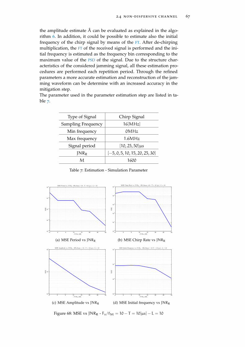
2.4 non-dispersive channel 67
the amplitude estimate A can be evaluated as explained in the algo-rithm 6. In addition, it could be possible to estimate also the initialfrequency of the chirp signal by means of the FT. After de-chirpingmultiplication, the FT of the received signal is performed and the ini-tial frequency is estimated as the frequency bin corresponding to themaximum value of the PSD of the signal. Due to the structure char-acteristics of the considered jamming signal, all these estimation pro-cedures are performed each repetition period. Through the refinedparameters a more accurate estimation and reconstruction of the jam-ming waveform can be determine with an increased accuracy in themitigation step.The parameter used in the parameter estimation step are listed in ta-ble 7.
Type of Signal Chirp Signal
Sampling Frequency 16[MHz]
Min frequency 0MHz
Max frequency 1.6MHz
Signal period [10, 25, 50]µs
JNRR [−5, 0, 5, 10, 15, 20, 25, 30]
M 1600
Table 7: Estimation - Simulation Parameter
−5 0 5 10 15 20 25 3010
−13
10−12
10−11
10−10
10−9
MSE Period vs JNRR- @Fs/fmax =10 - T =10 [µs] - L = 10
JNRR [dB]
MSE
(a) MSE Period vs JNRR
−5 0 5 10 15 20 25 3010
−8
10−7
10−6
10−5
10−4
10−3
MSE Chirp Rate vs JNRR - @Fs/fmax =10 - T = 10 [µs] - L = 10
JNRR [dB]
MSE
(b) MSE Chirp Rate vs JNRR
−5 0 5 10 15 20 25 3010
−2
10−1
100
MSE Amplitude vs JNRR - @Fs/fmax = 10 - T = 10 [µs] - L = 10
JNRR [dB]
MSE
(c) MSE Amplitude vs JNRR
−5 0 5 10 15 20 25 3010
−9
10−8
10−7
10−6
MSE Initial Frequency vs JNRR - @Fs/fmax = 10 T = 10 [µs] - L = 10
JNRR [dB]
MSE
(d) MSE Initial frequency vs JNRR
Figure 68: MSE vs JNRR - Fs/fM = 10− T = 10[µs] − L = 10
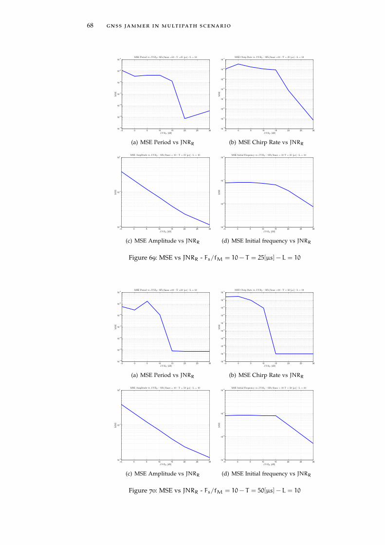
68 gnss jammer in multipath scenario
−5 0 5 10 15 20 25 3010
−14
10−13
10−12
10−11
10−10
10−9
10−8
MSE Period vs JNRR- @Fs/fmax =10 - T =25 [µs] - L = 10
JNRR [dB]
MSE
(a) MSE Period vs JNRR
−5 0 5 10 15 20 25 3010
−10
10−9
10−8
10−7
10−6
10−5
10−4
10−3
MSE Chirp Rate vs JNRR - @Fs/fmax =10 - T = 25 [µs] - L = 10
JNRR [dB]
MSE
(b) MSE Chirp Rate vs JNRR
−5 0 5 10 15 20 25 3010
−2
10−1
100
MSE Amplitude vs JNRR - @Fs/fmax = 10 - T = 25 [µs] - L = 10
JNRR [dB]
MSE
(c) MSE Amplitude vs JNRR
−5 0 5 10 15 20 25 3010
−9
10−8
10−7
10−6
MSE Initial Frequency vs JNRR - @Fs/fmax = 10 T = 25 [µs] - L = 10
JNRR [dB]
MSE
(d) MSE Initial frequency vs JNRR
Figure 69: MSE vs JNRR - Fs/fM = 10− T = 25[µs] − L = 10
−5 0 5 10 15 20 25 3010
−14
10−13
10−12
10−11
10−10
10−9
10−8
MSE Period vs JNRR- @Fs/fmax =10 - T =50 [µs] - L = 10
JNRR [dB]
MSE
(a) MSE Period vs JNRR
−5 0 5 10 15 20 25 3010
−12
10−11
10−10
10−9
10−8
10−7
10−6
10−5
10−4
10−3
MSE Chirp Rate vs JNRR - @Fs/fmax =10 - T = 50 [µs] - L = 10
JNRR [dB]
MSE
(b) MSE Chirp Rate vs JNRR
−5 0 5 10 15 20 25 3010
−2
10−1
100
MSE Amplitude vs JNRR - @Fs/fmax = 10 - T = 50 [µs] - L = 10
JNRR [dB]
MSE
(c) MSE Amplitude vs JNRR
−5 0 5 10 15 20 25 3010
−9
10−8
10−7
10−6
MSE Initial Frequency vs JNRR - @Fs/fmax = 10 T = 50 [µs] - L = 10
JNRR [dB]
MSE
(d) MSE Initial frequency vs JNRR
Figure 70: MSE vs JNRR - Fs/fM = 10− T = 50[µs] − L = 10
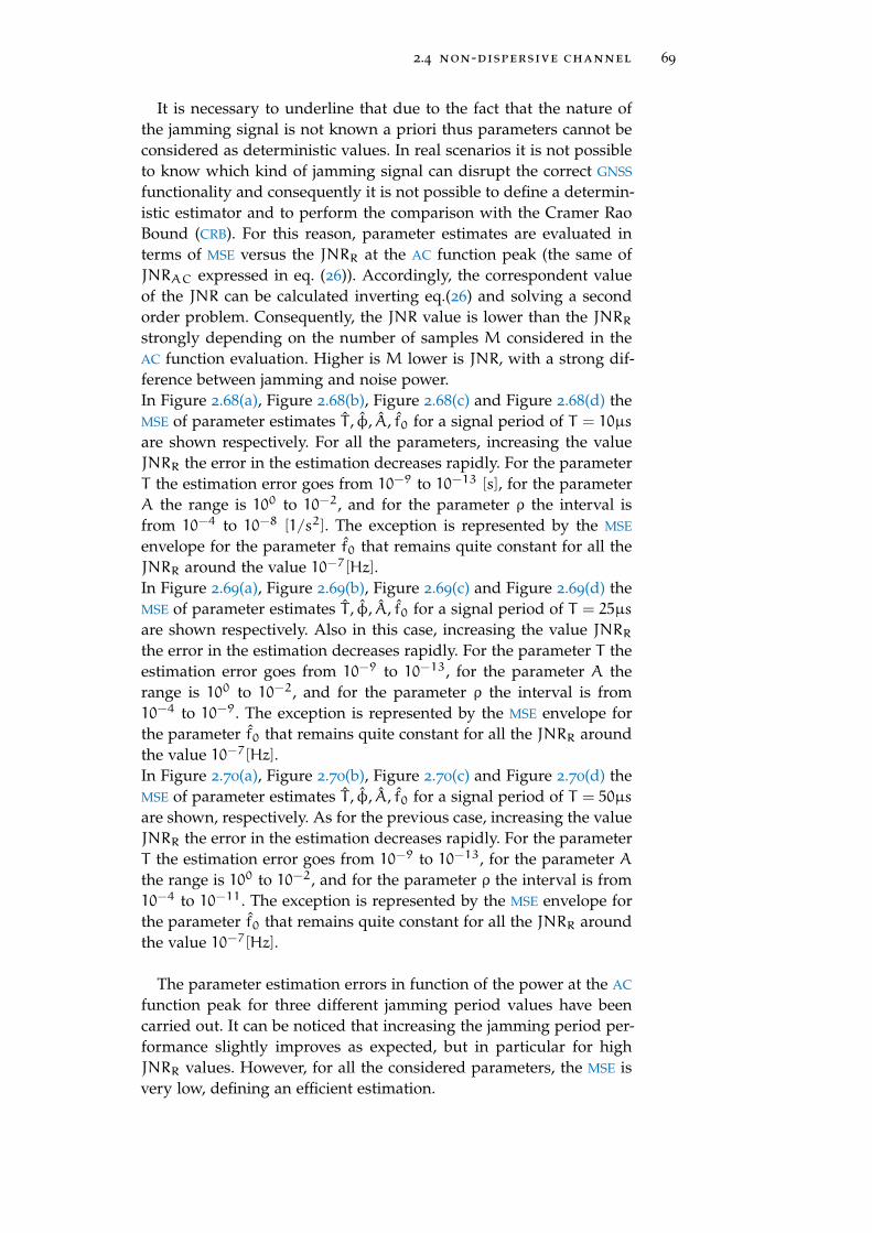
2.4 non-dispersive channel 69
It is necessary to underline that due to the fact that the nature ofthe jamming signal is not known a priori thus parameters cannot beconsidered as deterministic values. In real scenarios it is not possibleto know which kind of jamming signal can disrupt the correct GNSS
functionality and consequently it is not possible to define a determin-istic estimator and to perform the comparison with the Cramer RaoBound (CRB). For this reason, parameter estimates are evaluated interms of MSE versus the JNRR at the AC function peak (the same ofJNRAC expressed in eq. (26)). Accordingly, the correspondent valueof the JNR can be calculated inverting eq.(26) and solving a secondorder problem. Consequently, the JNR value is lower than the JNRRstrongly depending on the number of samples M considered in theAC function evaluation. Higher is M lower is JNR, with a strong dif-ference between jamming and noise power.In Figure 2.68(a), Figure 2.68(b), Figure 2.68(c) and Figure 2.68(d) theMSE of parameter estimates T , φ, A, f0 for a signal period of T = 10µs
are shown respectively. For all the parameters, increasing the valueJNRR the error in the estimation decreases rapidly. For the parameterT the estimation error goes from 10−9 to 10−13 [s], for the parameterA the range is 100 to 10−2, and for the parameter ρ the interval isfrom 10−4 to 10−8 [1/s2]. The exception is represented by the MSE
envelope for the parameter f0 that remains quite constant for all theJNRR around the value 10−7[Hz].In Figure 2.69(a), Figure 2.69(b), Figure 2.69(c) and Figure 2.69(d) theMSE of parameter estimates T , φ, A, f0 for a signal period of T = 25µs
are shown respectively. Also in this case, increasing the value JNRRthe error in the estimation decreases rapidly. For the parameter T theestimation error goes from 10−9 to 10−13, for the parameter A therange is 100 to 10−2, and for the parameter ρ the interval is from10−4 to 10−9. The exception is represented by the MSE envelope forthe parameter f0 that remains quite constant for all the JNRR aroundthe value 10−7[Hz].In Figure 2.70(a), Figure 2.70(b), Figure 2.70(c) and Figure 2.70(d) theMSE of parameter estimates T , φ, A, f0 for a signal period of T = 50µs
are shown, respectively. As for the previous case, increasing the valueJNRR the error in the estimation decreases rapidly. For the parameterT the estimation error goes from 10−9 to 10−13, for the parameter Athe range is 100 to 10−2, and for the parameter ρ the interval is from10−4 to 10−11. The exception is represented by the MSE envelope forthe parameter f0 that remains quite constant for all the JNRR aroundthe value 10−7[Hz].
The parameter estimation errors in function of the power at the AC
function peak for three different jamming period values have beencarried out. It can be noticed that increasing the jamming period per-formance slightly improves as expected, but in particular for highJNRR values. However, for all the considered parameters, the MSE isvery low, defining an efficient estimation.
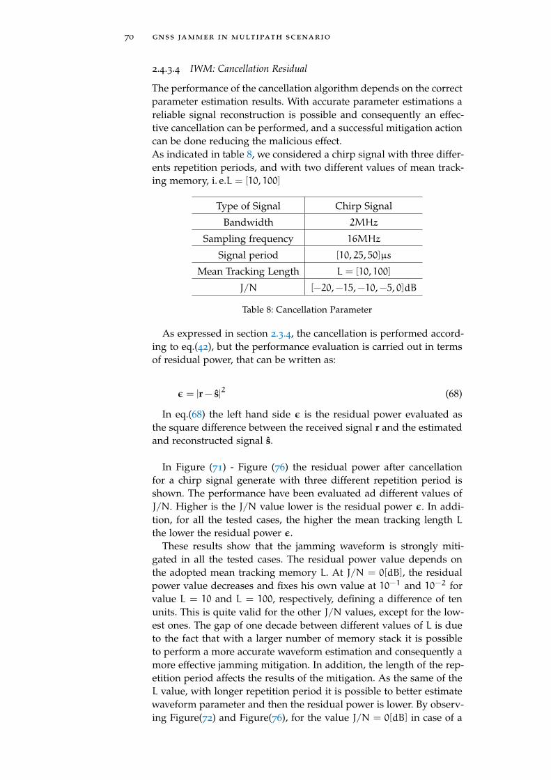
70 gnss jammer in multipath scenario
2.4.3.4 IWM: Cancellation Residual
The performance of the cancellation algorithm depends on the correctparameter estimation results. With accurate parameter estimations areliable signal reconstruction is possible and consequently an effec-tive cancellation can be performed, and a successful mitigation actioncan be done reducing the malicious effect.As indicated in table 8, we considered a chirp signal with three differ-ents repetition periods, and with two different values of mean track-ing memory, i. e.L = [10, 100]
Type of Signal Chirp Signal
Bandwidth 2MHz
Sampling frequency 16MHz
Signal period [10, 25, 50]µs
Mean Tracking Length L = [10, 100]
J/N [−20,−15,−10,−5, 0]dB
Table 8: Cancellation Parameter
As expressed in section 2.3.4, the cancellation is performed accord-ing to eq.(42), but the performance evaluation is carried out in termsof residual power, that can be written as:
ε = |r − s|2 (68)
In eq.(68) the left hand side ε is the residual power evaluated asthe square difference between the received signal r and the estimatedand reconstructed signal s.
In Figure (71) - Figure (76) the residual power after cancellationfor a chirp signal generate with three different repetition period isshown. The performance have been evaluated ad different values ofJ/N. Higher is the J/N value lower is the residual power ε. In addi-tion, for all the tested cases, the higher the mean tracking length Lthe lower the residual power ε.
These results show that the jamming waveform is strongly miti-gated in all the tested cases. The residual power value depends onthe adopted mean tracking memory L. At J/N = 0[dB], the residualpower value decreases and fixes his own value at 10−1 and 10−2 forvalue L = 10 and L = 100, respectively, defining a difference of tenunits. This is quite valid for the other J/N values, except for the low-est ones. The gap of one decade between different values of L is dueto the fact that with a larger number of memory stack it is possibleto perform a more accurate waveform estimation and consequently amore effective jamming mitigation. In addition, the length of the rep-etition period affects the results of the mitigation. As the same of theL value, with longer repetition period it is possible to better estimatewaveform parameter and then the residual power is lower. By observ-ing Figure(72) and Figure(76), for the value J/N = 0[dB] in case of a
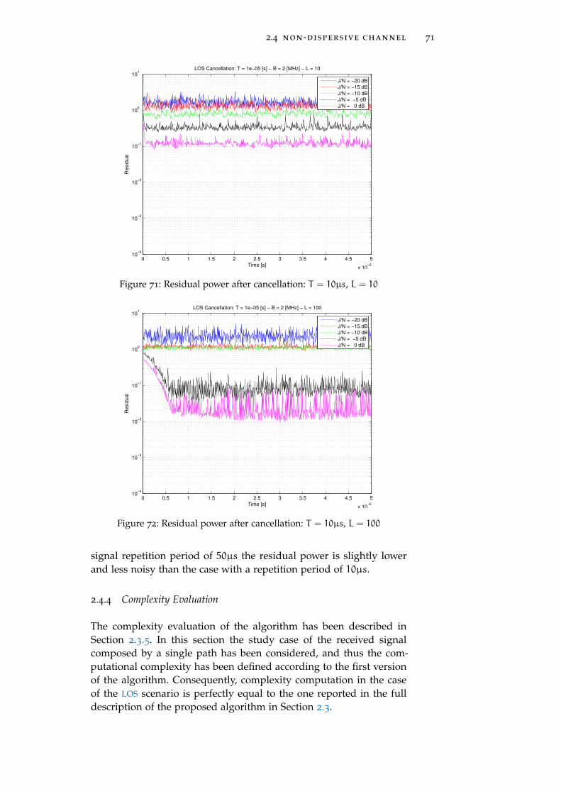
2.4 non-dispersive channel 71
0 0.5 1 1.5 2 2.5 3 3.5 4 4.5 5
x 10−5
10−4
10−3
10−2
10−1
100
101
Time [s]
Re
sid
ua
l
LOS Cancellation: T = 1e−05 [s] − B = 2 [MHz] − L = 10
J/N = −20 dB
J/N = −15 dB
J/N = −10 dB
J/N = −5 dB
J/N = 0 dB
Figure 71: Residual power after cancellation: T = 10µs, L = 10
0 0.5 1 1.5 2 2.5 3 3.5 4 4.5 5
x 10−5
10−4
10−3
10−2
10−1
100
101
Time [s]
Re
sid
ua
l
LOS Cancellation: T = 1e−05 [s] − B = 2 [MHz] − L = 100
J/N = −20 dB
J/N = −15 dB
J/N = −10 dB
J/N = −5 dB
J/N = 0 dB
Figure 72: Residual power after cancellation: T = 10µs, L = 100
signal repetition period of 50µs the residual power is slightly lowerand less noisy than the case with a repetition period of 10µs.
2.4.4 Complexity Evaluation
The complexity evaluation of the algorithm has been described inSection 2.3.5. In this section the study case of the received signalcomposed by a single path has been considered, and thus the com-putational complexity has been defined according to the first versionof the algorithm. Consequently, complexity computation in the caseof the LOS scenario is perfectly equal to the one reported in the fulldescription of the proposed algorithm in Section 2.3.
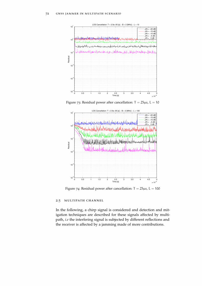
72 gnss jammer in multipath scenario
0 0.5 1 1.5 2 2.5 3 3.5 4 4.5 5
x 10−5
10−4
10−3
10−2
10−1
100
101
Time [s]
Re
sid
ua
l
LOS Cancellation: T = 2.5e−05 [s] − B = 2 [MHz] − L = 10
J/N = −20 dB
J/N = −15 dB
J/N = −10 dB
J/N = −5 dB
J/N = 0 dB
Figure 73: Residual power after cancellation: T = 25µs, L = 10
0 0.5 1 1.5 2 2.5 3 3.5 4 4.5 5
x 10−5
10−4
10−3
10−2
10−1
100
101
Time [s]
Re
sid
ua
l
LOS Cancellation: T = 2.5e−05 [s] − B = 2 [MHz] − L = 100
J/N = −20 dB
J/N = −15 dB
J/N = −10 dB
J/N = −5 dB
J/N = 0 dB
Figure 74: Residual power after cancellation: T = 25µs, L = 100
2.5 multipath channel
In the following, a chirp signal is considered and detection and mit-igation techniques are described for these signals affected by multi-path, i.e the interfering signal is subjected by different reflections andthe receiver is affected by a jamming made of more contributions.
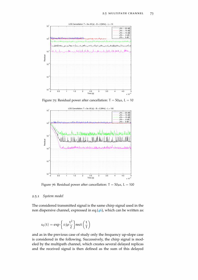
2.5 multipath channel 73
0 0.5 1 1.5 2 2.5 3 3.5 4 4.5 5
x 10−5
10−4
10−3
10−2
10−1
100
101
Time [s]
Re
sid
ua
l
LOS Cancellation: T = 5e−05 [s] − B = 2 [MHz] − L = 10
J/N = −20 dB
J/N = −15 dB
J/N = −10 dB
J/N = −5 dB
J/N = 0 dB
Figure 75: Residual power after cancellation: T = 50µs, L = 10
0 0.5 1 1.5 2 2.5 3 3.5 4 4.5 5
x 10−5
10−4
10−3
10−2
10−1
100
101
Time [s]
Re
sid
ua
l
LOS Cancellation: T = 5e−05 [s] − B = 2 [MHz] − L = 100
J/N = −20 dB
J/N = −15 dB
J/N = −10 dB
J/N = −5 dB
J/N = 0 dB
Figure 76: Residual power after cancellation: T = 50µs, L = 100
2.5.1 System model
The considered transmitted signal is the same chirp signal used in thenon dispersive channel, expressed in eq.(46), which can be written as:
s0(t) = exp{±jρt
2
2
}rect
(t
T
)and as in the previous case of study only the frequency up-slope caseis considered in the following. Successively, the chirp signal is mod-eled by the multipath channel, which creates several delayed replicasand the received signal is then defined as the sum of this delayed
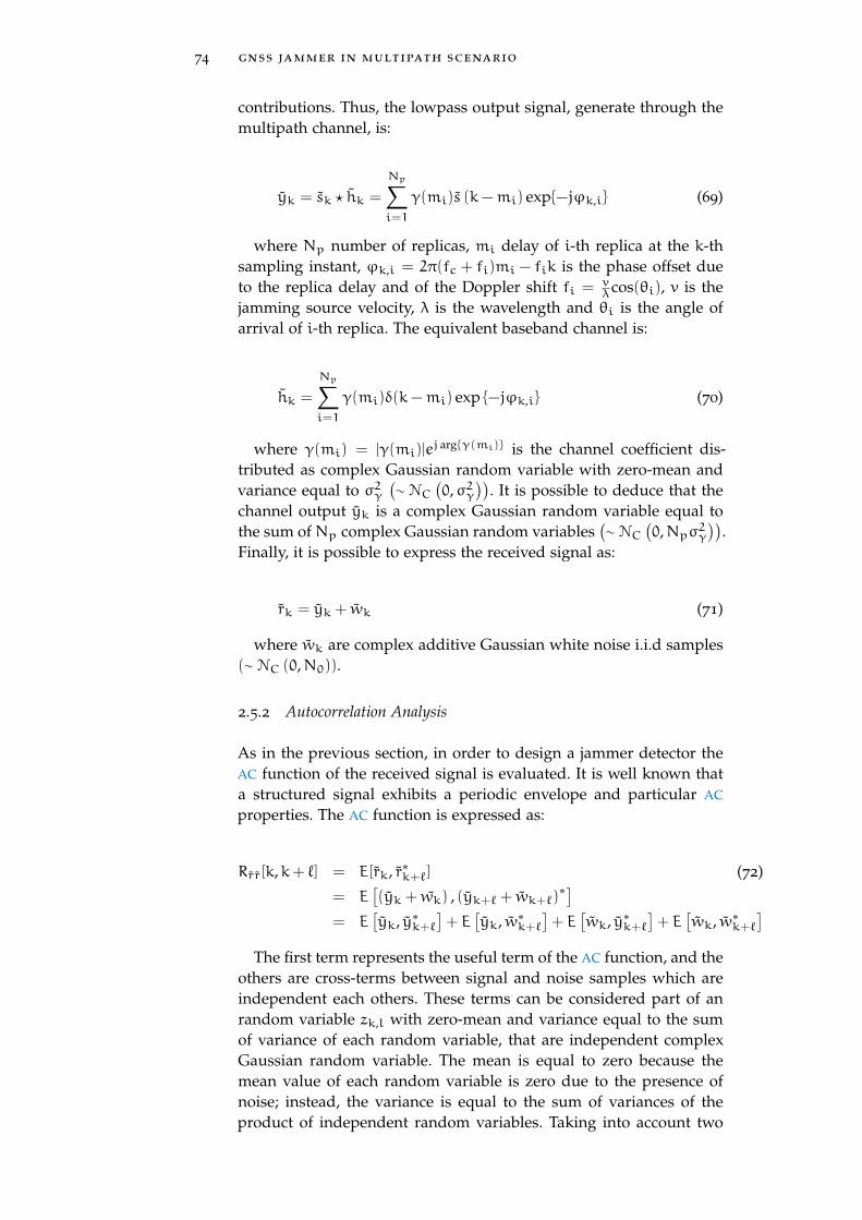
74 gnss jammer in multipath scenario
contributions. Thus, the lowpass output signal, generate through themultipath channel, is:
yk = sk ? hk =
Np∑i=1
γ(mi)s (k−mi) exp{−jϕk,i} (69)
where Np number of replicas, mi delay of i-th replica at the k-thsampling instant, ϕk,i = 2π(fc + fi)mi − fik is the phase offset dueto the replica delay and of the Doppler shift fi = v
λcos(θi), v is thejamming source velocity, λ is the wavelength and θi is the angle ofarrival of i-th replica. The equivalent baseband channel is:
hk =
Np∑i=1
γ(mi)δ(k−mi) exp {−jϕk,i} (70)
where γ(mi) = |γ(mi)|ej arg{γ(mi)} is the channel coefficient dis-
tributed as complex Gaussian random variable with zero-mean andvariance equal to σ2γ
(∼ NC
(0,σ2γ
)). It is possible to deduce that the
channel output yk is a complex Gaussian random variable equal tothe sum ofNp complex Gaussian random variables
(∼ NC
(0,Npσ2γ
)).
Finally, it is possible to express the received signal as:
rk = yk + wk (71)
where wk are complex additive Gaussian white noise i.i.d samples(∼ NC (0,N0)).
2.5.2 Autocorrelation Analysis
As in the previous section, in order to design a jammer detector theAC function of the received signal is evaluated. It is well known thata structured signal exhibits a periodic envelope and particular AC
properties. The AC function is expressed as:
Rrr[k,k+ `] = E[rk, r∗k+`] (72)
= E[(yk + wk) , (yk+` + wk+`)
∗]= E
[yk, y∗k+`
]+ E
[yk, w∗k+`
]+ E
[wk, y∗k+`
]+ E
[wk, w∗k+`
]The first term represents the useful term of the AC function, and the
others are cross-terms between signal and noise samples which areindependent each others. These terms can be considered part of anrandom variable zk,l with zero-mean and variance equal to the sumof variance of each random variable, that are independent complexGaussian random variable. The mean is equal to zero because themean value of each random variable is zero due to the presence ofnoise; instead, the variance is equal to the sum of variances of theproduct of independent random variables. Taking into account two

2.5 multipath channel 75
independent random variable a,b as in Section 2.3.1.1, the varianceof their product is evaluated as:
Var{ab} = Var{a}Var{b}+ E2[a]Var{b}+ E2[b]Var{a} (73)
The variance of each product is:
Var{ykw∗k+`} =
Np∑i=1
σ2γ,i ∗N0 (74)
Var{wky∗k+`} =
Np∑i=1
σ2γ,i ∗N0
Var{wkw∗k+`} = N20
and the variance of the total random variable zk,l is
Var{zk,l} = N0(2
Np∑i=1
σ2γ,i +N0) (75)
It is worthwhile to notice that assuming the channel coefficients γindependent each others then the variance Var{yk} can be expressedas
Var{yk} =
Np∑i=1
σ2γ,i
; on the other hand if coefficients are not independent the variance isexpressed as
Var{yk} = Var{
Np∑i=1
γi}
The first term of the AC function is defined as the product of twoindependent complex Gaussian random variables:
Ryy[k,k+ `] = E[yk, y∗k+`
](76)
= E
Np∑i=1
γ(mi)s(k−mi)e−jϕk,i
·Np∑q=1
γ∗(mq)s∗(k−mq + `)e
jϕk+`,q
Taking into account that the channel is static and that into the time-
period T the Doppler shift due to the jamming source velocity is notrelevant, then the estimated AC function can be evaluated through thearithmetic mean:
Ryy[`] =1
L− `
L−∑k=1
Np∑i=1
γ(mi)s(k−mi)e−jϕk,i (77)
·Np∑p=1
γ∗(mp)s∗(k−mp + `)e
jϕk+`,p
76 gnss jammer in multipath scenario
Thus:
Ryy[`] =1
L− `
L−∑k=1
Np∑i=1
h(mi)s(k−mi) ·Np∑q=1
h∗(mq)x∗(k−mq + `)
(78)
=
Np∑i=1
Np∑q=1
h(mi)h∗(mq) ·
1
L− `
L−∑k=1
s(k−mi)s∗(k−mq + `)
=
Np∑i=1
Np∑q=1
h(mi)h∗(mq)Rss[`−mq +mi]
According to eq.(78) the estimated AC function Ryy[`] of the re-ceived signal can be expressed as the linear combination of the AC ofthe transmitted signal affected by multipath Rss weighted by channelcoefficients. In order to estimate the period of the transmitted signal,it is necessary to evaluate the maximum value of the correlation func-tion, rejecting the first maximum corresponding to the beginning ofthe signal: the correspondent instant is equal to the value of the sig-nal period. In this case with a signal affected by Np paths the numberof all the contributions in eq.(78) are N2p: the maximum value corre-sponds to the case of perfect alignment of the received signal andits delayed replicas, while the other combinations contribute to sec-ondary lobes in the AC function. The expression in eq.(78) is a closedform but it is not an explicit form, so in order to demonstrate thebehavior of the AC function it is necessary to evaluate empirically allthe possible cases of alignment of the paths.
2.5.3 Detector Design
The next step is to define the analytic expression of the decision prob-lem regarding the detection of the correct signal period. The detectionproblem is defined as a binary decision problem, which is composedby two hypotheses:
• H1:maximum pick of the AC function. The time instant ( 6= 0)
corresponding to the maximum pick is a multiple of the signalperiod, obtained when the replicas are perfectly aligned.
• H0:maximum pick is absent. There are secondary picks due tothe several cross-overlapping of the replicas. The assumption isthat the AC function is 0.
The AC function of the received signal in eq.(72), can be rewritten as:
Rrr(`) =
Np∑i=1
Np∑q=1
h(mi)h∗(mq)Rss[`−mq +mi] + RW(`) (79)
where the term RW(`) represents all the contributions due to thecross-correlation between signal and noise and the noise autocorrela-tion function. It is necessary to evaluate the expression of this func-
2.5 multipath channel 77
tion under both hypotheses. Under H1 we consider the perfect align-ment of the received signal and its local replicas. According to this, itis possible to derive:
∣∣∣∣∣∣∣Np∑i=1i=q
|h(mi)|2 Rss(`) + RW(`)
∣∣∣∣∣∣∣2
(80)
where:
• RW(`) can be modeled as a Gaussian random variable: RW(`) ∼
N(0,N0)
• Rss(`) is deterministic equal to the signal energy E under H1and equal to 0 under H0
• |h(mi)|2 can be considered as a random variable o a determin-
istic value
– deterministic value: each term represents the energy of thei-th delay;
– random variable: the sum of all these quadratic terms canbe modeled as a non central chi-square distribution.
2.5.3.1 Deterministic Channel Distribution
In this paragraph the analytic expression of the decision problem in adeterministic case is evaluated. Assuming that |h(mi)|
2 is a determin-istic value, the sufficient statistics, under H1 hypothesis, is expressedas a non central chi-square random variable with 2L degrees of free-dom χ22L(d), with non centrality parameter given by:
d =
∣∣∣∣∣∣∣Np∑i=1i=q
|h(mi)|2 Rss(`|H1)
∣∣∣∣∣∣∣2
(81)
=
∣∣∣∣∣∣∣Np∑i=1i=q
|h(mi)|2 Eejφ
∣∣∣∣∣∣∣2
=∑i=1i=q
Np
|h(mi)|4 E2 + 2
Np∑j=1
Np∑i=1j6=i
|h(mi)|2∣∣h(mj)∣∣2 E2
Under H0 hypothesis the sufficient statistic is expressed as a cen-
tral chi-square random variable with 2L degrees of freedom χ22L(0).Taking into account that under H0 the AC function of the interferingsignal Rss(`) is equal to 0, then the sufficient statistic is composedby noise contribution RW which is modeled as a complex Gaussianrandom variable.
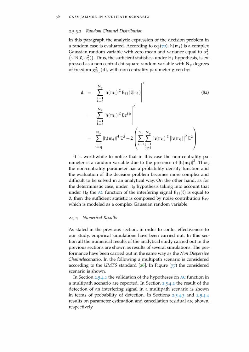
78 gnss jammer in multipath scenario
2.5.3.2 Random Channel Distribution
In this paragraph the analytic expression of the decision problem ina random case is evaluated. According to eq.(70), h(mi) is a complexGaussian random variable with zero mean and variance equal to σ2γ(∼ N(0,σ2γ)
). Thus, the sufficient statistics, under H1 hypothesis, is ex-
pressed as a non central chi-square random variable with Np degreesof freedom χ2Np(d), with non centrality parameter given by:
d =
∣∣∣∣∣∣∣Np∑i=1i=q
|h(mi)|2 Rss(`|H1)
∣∣∣∣∣∣∣2
(82)
=
∣∣∣∣∣∣∣Np∑i=1i=q
|h(mi)|2 Eejφ
∣∣∣∣∣∣∣2
=
Np∑i=1i=q
|h(mi)|4 E2 + 2
Np∑i=1
Np∑j=1j6=i
|h(mi)|2∣∣h(mj)∣∣2 E2
It is worthwhile to notice that in this case the non centrality pa-
rameter is a random variable due to the presence of |h(mi)|2. Thus,
the non-centrality parameter has a probability density function andthe evaluation of the decision problem becomes more complex anddifficult to be solved in an analytical way. On the other hand, as forthe deterministic case, under H0 hypothesis taking into account thatunder H0 the AC function of the interfering signal Rss(`) is equal to0, then the sufficient statistic is composed by noise contribution RWwhich is modeled as a complex Gaussian random variable.
2.5.4 Numerical Results
As stated in the previous section, in order to confer effectiveness toour study, empirical simulations have been carried out. In this sec-tion all the numerical results of the analytical study carried out in theprevious sections are shown as results of several simulations. The per-formance have been carried out in the same way as the Non DispersiveChannelscenario. In the following a multipath scenario is consideredaccording to the UMTS standard [26]. In Figure (77) the consideredscenario is shown.
In Section 2.5.4.1 the validation of the hypotheses on AC function ina multipath scenario are reported. In Section 2.5.4.2 the result of thedetection of an interfering signal in a multipath scenario is shownin terms of probability of detection. In Sections 2.5.4.3 and 2.5.4.4results on parameter estimation and cancellation residual are shown,respectively.
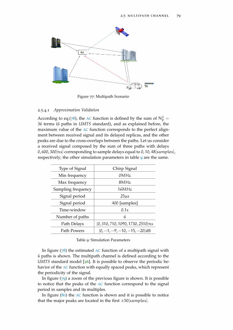
2.5 multipath channel 79
Figure 77: Multipath Scenario
2.5.4.1 Approximation Validation
According to eq.(78), the AC function is defined by the sum of N2p =
36 terms (6 paths in UMTS standard), and as explained before, themaximum value of the AC function corresponds to the perfect align-ment between received signal and its delayed replicas, and the otherpeaks are due to the cross-overlaps between the paths. Let us considera received signal composed by the sum of three paths with delays0, 600, 300[ns] corresponding to sample delays equal to 0, 10, 48[samples],respectively; the other simulation parameters in table 9 are the same.
Type of Signal Chirp Signal
Min frequency 0MHz
Max frequency 8MHz
Sampling frequency 16MHz
Signal period 25µs
Signal period 400 [samples]
Time-window 0.1s
Number of paths 6
Path Delays [0, 310, 710, 1090, 1730, 2510]ns
Path Powers [0,−1,−9,−10,−15,−20]dB
Table 9: Simulation Parameters
In figure (78) the estimated AC function of a multipath signal with6 paths is shown. The multipath channel is defined according to theUMTS standard model [26]. It is possible to observe the periodic be-havior of the AC function with equally spaced peaks, which representthe periodicity of the signal.
In figure (79) a zoom of the previous figure is shown. It is possibleto notice that the peaks of the AC function correspond to the signalperiod in samples and its multiples.
In figure (80) the AC function is shown and it is possible to noticethat the major peaks are located in the first ±50[samples].
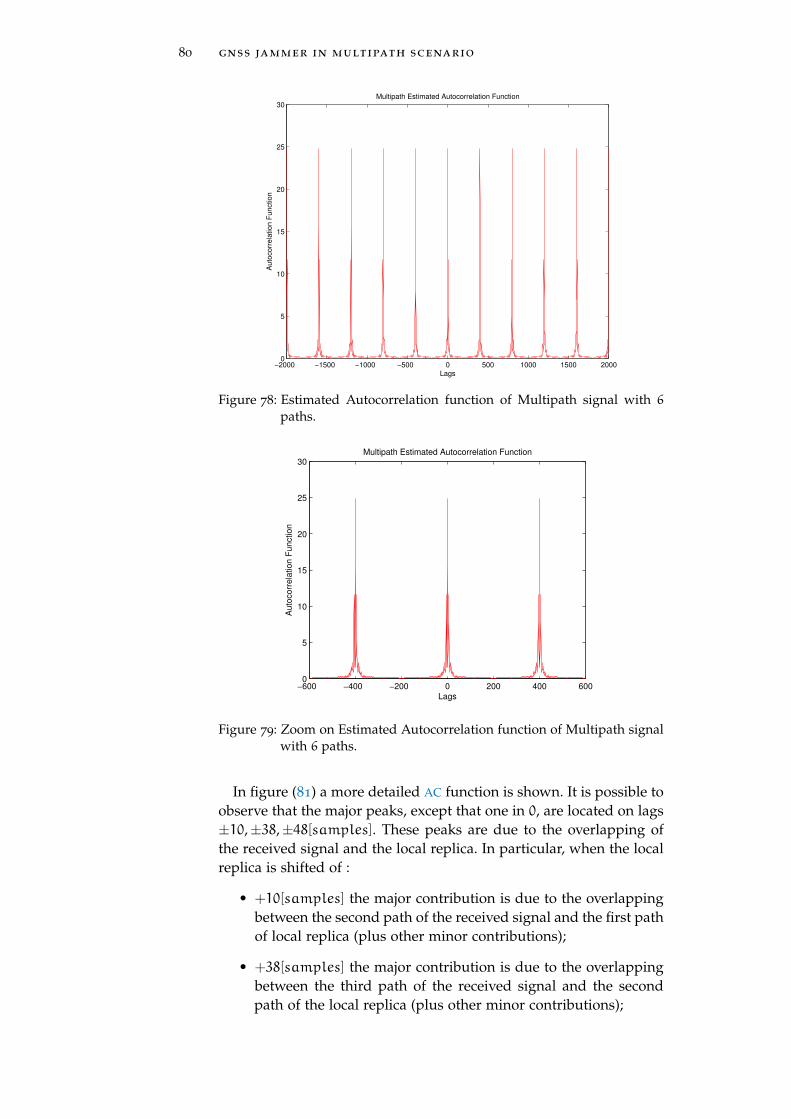
80 gnss jammer in multipath scenario
−2000 −1500 −1000 −500 0 500 1000 1500 20000
5
10
15
20
25
30
Lags
Au
toco
rre
latio
n F
un
ctio
n
Multipath Estimated Autocorrelation Function
Figure 78: Estimated Autocorrelation function of Multipath signal with 6
paths.
−600 −400 −200 0 200 400 6000
5
10
15
20
25
30
Lags
Au
toco
rre
latio
n F
un
ctio
n
Multipath Estimated Autocorrelation Function
Figure 79: Zoom on Estimated Autocorrelation function of Multipath signalwith 6 paths.
In figure (81) a more detailed AC function is shown. It is possible toobserve that the major peaks, except that one in 0, are located on lags±10,±38,±48[samples]. These peaks are due to the overlapping ofthe received signal and the local replica. In particular, when the localreplica is shifted of :
• +10[samples] the major contribution is due to the overlappingbetween the second path of the received signal and the first pathof local replica (plus other minor contributions);
• +38[samples] the major contribution is due to the overlappingbetween the third path of the received signal and the secondpath of the local replica (plus other minor contributions);
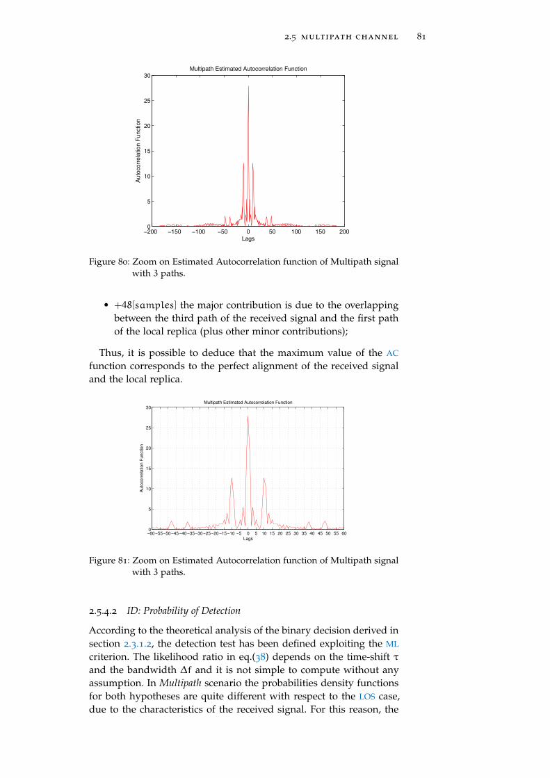
2.5 multipath channel 81
−200 −150 −100 −50 0 50 100 150 2000
5
10
15
20
25
30
Lags
Au
toco
rre
latio
n F
un
ctio
n
Multipath Estimated Autocorrelation Function
Figure 80: Zoom on Estimated Autocorrelation function of Multipath signalwith 3 paths.
• +48[samples] the major contribution is due to the overlappingbetween the third path of the received signal and the first pathof the local replica (plus other minor contributions);
Thus, it is possible to deduce that the maximum value of the AC
function corresponds to the perfect alignment of the received signaland the local replica.
−60−55−50−45−40−35−30−25−20−15−10 −5 0 5 10 15 20 25 30 35 40 45 50 55 600
5
10
15
20
25
30
Lags
Au
toco
rre
latio
n F
un
ctio
n
Multipath Estimated Autocorrelation Function
Figure 81: Zoom on Estimated Autocorrelation function of Multipath signalwith 3 paths.
2.5.4.2 ID: Probability of Detection
According to the theoretical analysis of the binary decision derived insection 2.3.1.2, the detection test has been defined exploiting the ML
criterion. The likelihood ratio in eq.(38) depends on the time-shift τand the bandwidth ∆f and it is not simple to compute without anyassumption. In Multipath scenario the probabilities density functionsfor both hypotheses are quite different with respect to the LOS case,due to the characteristics of the received signal. For this reason, the
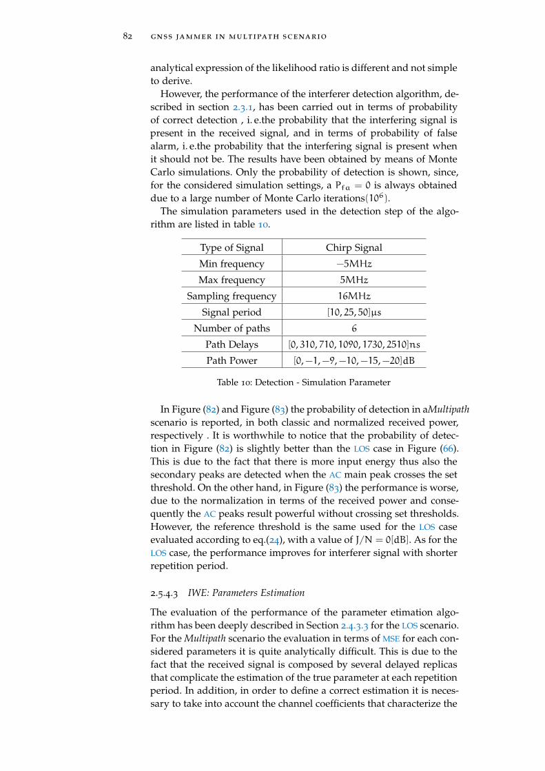
82 gnss jammer in multipath scenario
analytical expression of the likelihood ratio is different and not simpleto derive.
However, the performance of the interferer detection algorithm, de-scribed in section 2.3.1, has been carried out in terms of probabilityof correct detection , i. e.the probability that the interfering signal ispresent in the received signal, and in terms of probability of falsealarm, i. e.the probability that the interfering signal is present whenit should not be. The results have been obtained by means of MonteCarlo simulations. Only the probability of detection is shown, since,for the considered simulation settings, a Pfa = 0 is always obtaineddue to a large number of Monte Carlo iterations(106).
The simulation parameters used in the detection step of the algo-rithm are listed in table 10.
Type of Signal Chirp Signal
Min frequency −5MHz
Max frequency 5MHz
Sampling frequency 16MHz
Signal period [10, 25, 50]µs
Number of paths 6
Path Delays [0, 310, 710, 1090, 1730, 2510]ns
Path Power [0,−1,−9,−10,−15,−20]dB
Table 10: Detection - Simulation Parameter
In Figure (82) and Figure (83) the probability of detection in aMultipathscenario is reported, in both classic and normalized received power,respectively . It is worthwhile to notice that the probability of detec-tion in Figure (82) is slightly better than the LOS case in Figure (66).This is due to the fact that there is more input energy thus also thesecondary peaks are detected when the AC main peak crosses the setthreshold. On the other hand, in Figure (83) the performance is worse,due to the normalization in terms of the received power and conse-quently the AC peaks result powerful without crossing set thresholds.However, the reference threshold is the same used for the LOS caseevaluated according to eq.(24), with a value of J/N = 0[dB]. As for theLOS case, the performance improves for interferer signal with shorterrepetition period.
2.5.4.3 IWE: Parameters Estimation
The evaluation of the performance of the parameter etimation algo-rithm has been deeply described in Section 2.4.3.3 for the LOS scenario.For the Multipath scenario the evaluation in terms of MSE for each con-sidered parameters it is quite analytically difficult. This is due to thefact that the received signal is composed by several delayed replicasthat complicate the estimation of the true parameter at each repetitionperiod. In addition, in order to define a correct estimation it is neces-sary to take into account the channel coefficients that characterize the
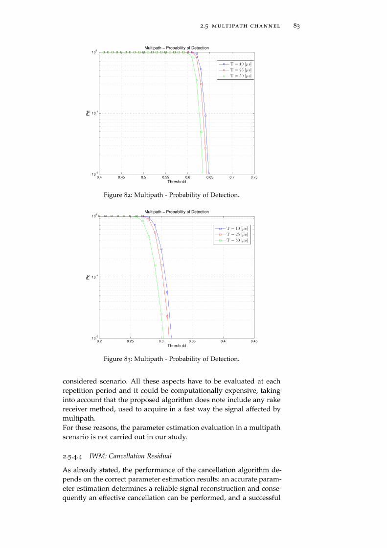
2.5 multipath channel 83
0.4 0.45 0.5 0.55 0.6 0.65 0.7 0.7510
−2
10−1
100
Threshold
Pd
Multipath − Probability of Detection
T = 10 [µs]
T = 25 [µs]
T = 50 [µs]
Figure 82: Multipath - Probability of Detection.
0.2 0.25 0.3 0.35 0.4 0.4510
−2
10−1
100
Threshold
Pd
Multipath − Probability of Detection
T = 10 [µs]
T = 25 [µs]
T = 50 [µs]
Figure 83: Multipath - Probability of Detection.
considered scenario. All these aspects have to be evaluated at eachrepetition period and it could be computationally expensive, takinginto account that the proposed algorithm does note include any rakereceiver method, used to acquire in a fast way the signal affected bymultipath.For these reasons, the parameter estimation evaluation in a multipathscenario is not carried out in our study.
2.5.4.4 IWM: Cancellation Residual
As already stated, the performance of the cancellation algorithm de-pends on the correct parameter estimation results: an accurate param-eter estimation determines a reliable signal reconstruction and conse-quently an effective cancellation can be performed, and a successful
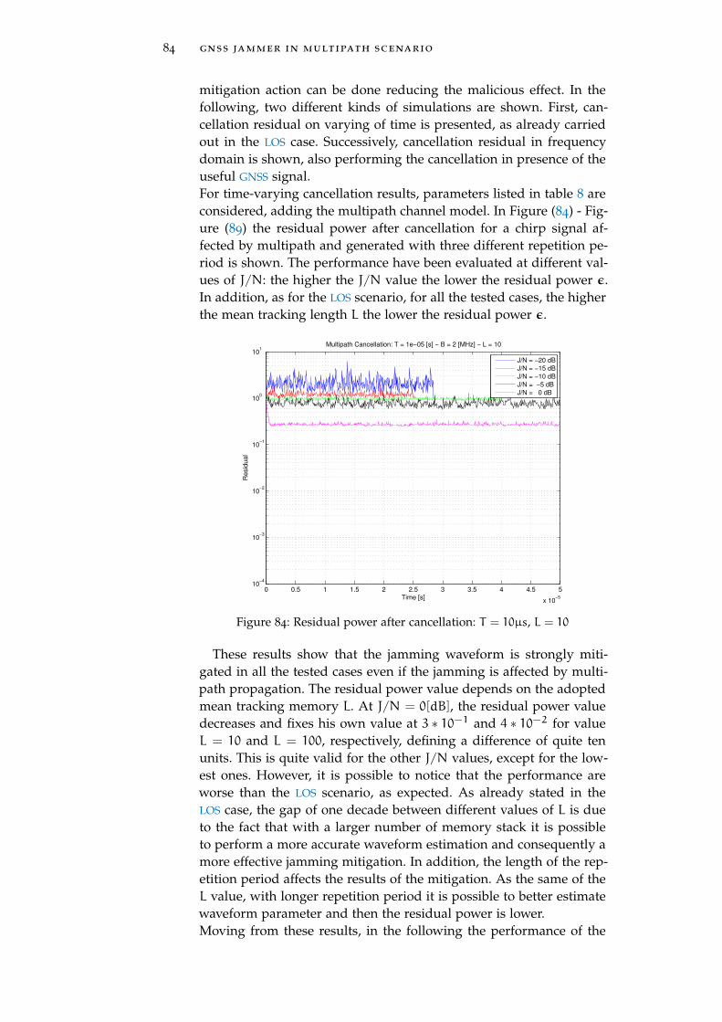
84 gnss jammer in multipath scenario
mitigation action can be done reducing the malicious effect. In thefollowing, two different kinds of simulations are shown. First, can-cellation residual on varying of time is presented, as already carriedout in the LOS case. Successively, cancellation residual in frequencydomain is shown, also performing the cancellation in presence of theuseful GNSS signal.For time-varying cancellation results, parameters listed in table 8 areconsidered, adding the multipath channel model. In Figure (84) - Fig-ure (89) the residual power after cancellation for a chirp signal af-fected by multipath and generated with three different repetition pe-riod is shown. The performance have been evaluated at different val-ues of J/N: the higher the J/N value the lower the residual power ε.In addition, as for the LOS scenario, for all the tested cases, the higherthe mean tracking length L the lower the residual power ε.
0 0.5 1 1.5 2 2.5 3 3.5 4 4.5 5
x 10−5
10−4
10−3
10−2
10−1
100
101
Time [s]
Re
sid
ua
l
Multipath Cancellation: T = 1e−05 [s] − B = 2 [MHz] − L = 10
J/N = −20 dB
J/N = −15 dB
J/N = −10 dB
J/N = −5 dB
J/N = 0 dB
Figure 84: Residual power after cancellation: T = 10µs, L = 10
These results show that the jamming waveform is strongly miti-gated in all the tested cases even if the jamming is affected by multi-path propagation. The residual power value depends on the adoptedmean tracking memory L. At J/N = 0[dB], the residual power valuedecreases and fixes his own value at 3 ∗ 10−1 and 4 ∗ 10−2 for valueL = 10 and L = 100, respectively, defining a difference of quite tenunits. This is quite valid for the other J/N values, except for the low-est ones. However, it is possible to notice that the performance areworse than the LOS scenario, as expected. As already stated in theLOS case, the gap of one decade between different values of L is dueto the fact that with a larger number of memory stack it is possibleto perform a more accurate waveform estimation and consequently amore effective jamming mitigation. In addition, the length of the rep-etition period affects the results of the mitigation. As the same of theL value, with longer repetition period it is possible to better estimatewaveform parameter and then the residual power is lower.Moving from these results, in the following the performance of the
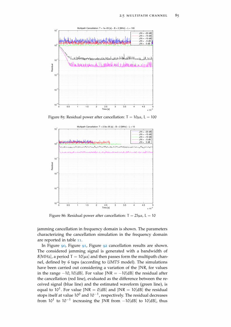
2.5 multipath channel 85
0 0.5 1 1.5 2 2.5 3 3.5 4 4.5 5
x 10−5
10−4
10−3
10−2
10−1
100
101
Time [s]
Re
sid
ua
l
Multipath Cancellation: T = 1e−05 [s] − B = 2 [MHz] − L = 100
J/N = −20 dB
J/N = −15 dB
J/N = −10 dB
J/N = −5 dB
J/N = 0 dB
Figure 85: Residual power after cancellation: T = 10µs, L = 100
0 0.5 1 1.5 2 2.5 3 3.5 4 4.5 5
x 10−5
10−4
10−3
10−2
10−1
100
101
Time [s]
Re
sid
ua
l
Multipath Cancellation: T = 2.5e−05 [s] − B = 2 [MHz] − L = 10
J/N = −20 dB
J/N = −15 dB
J/N = −10 dB
J/N = −5 dB
J/N = 0 dB
Figure 86: Residual power after cancellation: T = 25µs, L = 10
jamming cancellation in frequency domain is shown. The parameterscharacterizing the cancellation simulation in the frequency domainare reported in table 11.
In Figure 90, Figure 91, Figure 92 cancellation results are shown.The considered jamming signal is generated with a bandwidth of8[MHz], a period T = 10[µs] and then passes form the multipath chan-nel, defined by 6 taps (according to UMTS model). The simulationshave been carried out considering a variation of the JNR, for valuesin the range −10, 10[dB]. For value JNR = −10[dB] the residual afterthe cancellation (red line), evaluated as the difference between the re-ceived signal (blue line) and the estimated waveform (green line), isequal to 101. For value JNR = 0[dB] and JNR = 10[dB] the residualstops itself at value 100 and 10−1, respectively. The residual decreasesfrom 101 to 10−1 increasing the JNR from −10[dB] to 10[dB], thus
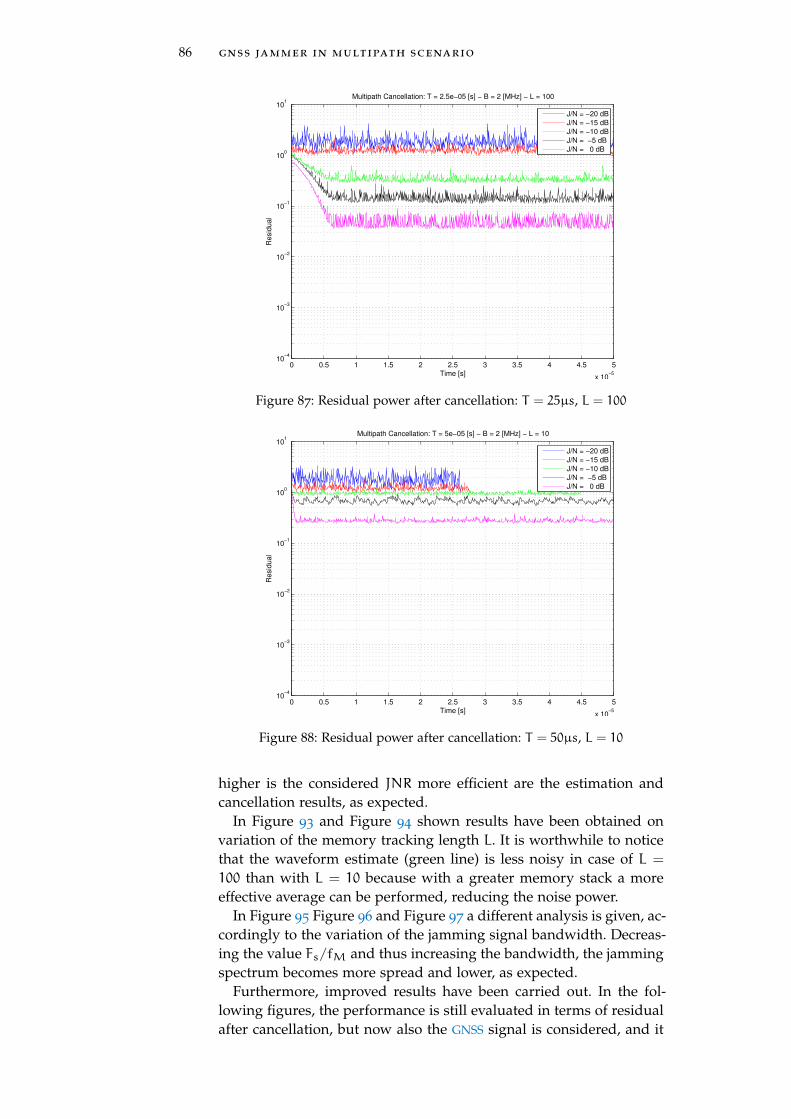
86 gnss jammer in multipath scenario
0 0.5 1 1.5 2 2.5 3 3.5 4 4.5 5
x 10−5
10−4
10−3
10−2
10−1
100
101
Time [s]
Re
sid
ua
l
Multipath Cancellation: T = 2.5e−05 [s] − B = 2 [MHz] − L = 100
J/N = −20 dB
J/N = −15 dB
J/N = −10 dB
J/N = −5 dB
J/N = 0 dB
Figure 87: Residual power after cancellation: T = 25µs, L = 100
0 0.5 1 1.5 2 2.5 3 3.5 4 4.5 5
x 10−5
10−4
10−3
10−2
10−1
100
101
Time [s]
Re
sid
ua
l
Multipath Cancellation: T = 5e−05 [s] − B = 2 [MHz] − L = 10
J/N = −20 dB
J/N = −15 dB
J/N = −10 dB
J/N = −5 dB
J/N = 0 dB
Figure 88: Residual power after cancellation: T = 50µs, L = 10
higher is the considered JNR more efficient are the estimation andcancellation results, as expected.
In Figure 93 and Figure 94 shown results have been obtained onvariation of the memory tracking length L. It is worthwhile to noticethat the waveform estimate (green line) is less noisy in case of L =
100 than with L = 10 because with a greater memory stack a moreeffective average can be performed, reducing the noise power.
In Figure 95 Figure 96 and Figure 97 a different analysis is given, ac-cordingly to the variation of the jamming signal bandwidth. Decreas-ing the value Fs/fM and thus increasing the bandwidth, the jammingspectrum becomes more spread and lower, as expected.
Furthermore, improved results have been carried out. In the fol-lowing figures, the performance is still evaluated in terms of residualafter cancellation, but now also the GNSS signal is considered, and it
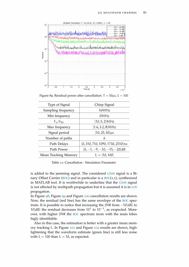
2.5 multipath channel 87
0 0.5 1 1.5 2 2.5 3 3.5 4 4.5 5
x 10−5
10−4
10−3
10−2
10−1
100
101
Time [s]
Re
sid
ua
l
Multipath Cancellation: T = 5e−05 [s] − B = 2 [MHz] − L = 100
J/N = −20 dB
J/N = −15 dB
J/N = −10 dB
J/N = −5 dB
J/N = 0 dB
Figure 89: Residual power after cancellation: T = 50µs, L = 100
Type of Signal Chirp Signal
Sampling frequency 16MHz
Min frequency 0MHz
Fs/fM [10, 5, 2]MHz
Max frequency [1.6, 3.2, 8]MHz
Signal period [10, 25, 50]µs
Number of paths 6
Path Delays [0, 310, 710, 1090, 1730, 2510]ns
Path Power [0,−1,−9,−10,−15,−20]dB
Mean Tracking Memory L = [10, 100]
Table 11: Cancellation - Simulation Parameter
is added to the jamming signal. The considered GNSS signal is a Bi-nary Offset Carrier (BOC) and in particular is a BOC(1,1), synthesizedin MATLAB tool. It is worthwhile to underline that the GNSS signalis not affected by multipath propagation but it is assumed it is in LOS
propagation.In Figure 98, Figure 99 and Figure 100 cancellation results are shown.Now, the residual (red line) has the same envelope of the BOC spec-trum. It is possible to notice that increasing the JNR from −10[dB] to10[dB] the residual decreases from 101 to 10−1, as exspected. More-over, with higher JNR the BOC spectrum more with the main lobeshigly identifiable.
Also in this case, the estimation is better with a greater mean mem-ory tracking L. In Figure 101 and Figure 102 results are shown, high-lightening that the waveform estimate (green line) is still less noisewith L = 100 than L = 10, as espected.
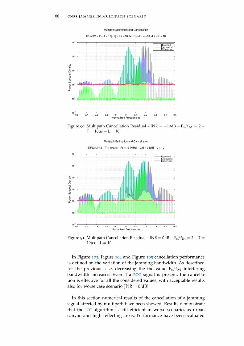
88 gnss jammer in multipath scenario
−0.5 −0.4 −0.3 −0.2 −0.1 0 0.1 0.2 0.3 0.4 0.510
−1
100
101
102
103
104
Multipath Estimation and Cancellation
@Fs2fM = 2 − T = 10[µ s] − Fs = 16 [MHz] − J/N = −10 [dB] − L = 10
Normalized Frequencies
Pow
er
Spect
ral D
ensi
ty
ReceivedEstimatedDifference
Figure 90: Multipath Cancellation Residual - JNR = −10dB− Fs/fM = 2−
T = 10µs− L = 10
−0.5 −0.4 −0.3 −0.2 −0.1 0 0.1 0.2 0.3 0.4 0.510
−2
10−1
100
101
102
103
104
Multipath Estimation and Cancellation
@Fs2fM = 2 − T = 10[µ s] − Fs = 16 [MHz] − J/N = 0 [dB] − L = 10
Normalized Frequencies
Pow
er
Spect
ral D
ensi
ty
ReceivedEstimatedDifference
Figure 91: Multipath Cancellation Residual - JNR = 0dB− Fs/fM = 2− T =
10µs− L = 10
In Figure 103, Figure 104 and Figure 105 cancellation performanceis defined on the variation of the jamming bandwidth. As describedfor the previous case, decreasing the the value Fs/fM interferingbandwidth increases. Even if a BOC signal is present, the cancella-tion is effective for all the considered values, with acceptable resultsalso for worse case scenario JNR = 0[dB].
In this section numerical results of the cancellation of a jammingsignal affected by multipath have been showed. Results demonstratethat the ICC algorithm is still efficient in worse scenario, as urbancanyon and high reflecting areas. Performance have been evaluated
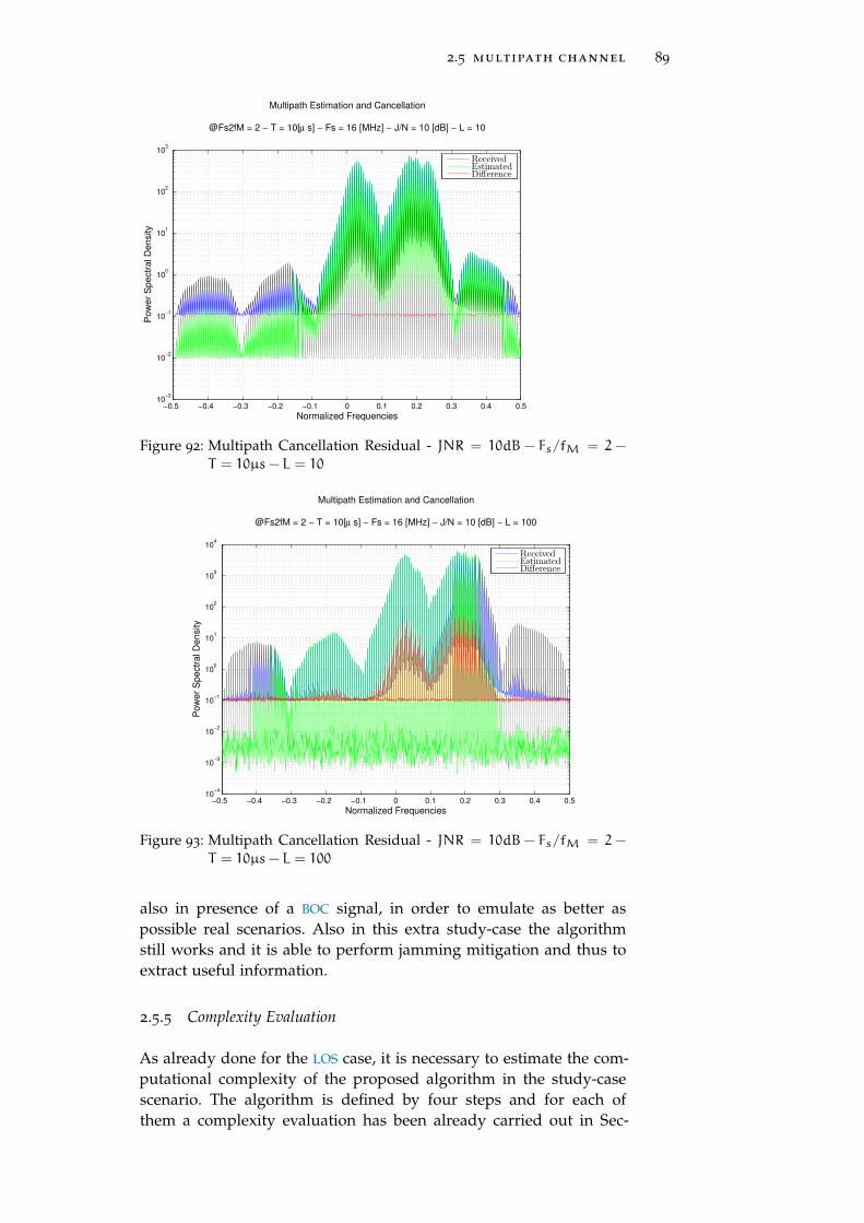
2.5 multipath channel 89
−0.5 −0.4 −0.3 −0.2 −0.1 0 0.1 0.2 0.3 0.4 0.510
−3
10−2
10−1
100
101
102
103
Multipath Estimation and Cancellation
@Fs2fM = 2 − T = 10[µ s] − Fs = 16 [MHz] − J/N = 10 [dB] − L = 10
Normalized Frequencies
Pow
er
Spect
ral D
ensi
ty
ReceivedEstimatedDifference
Figure 92: Multipath Cancellation Residual - JNR = 10dB − Fs/fM = 2 −
T = 10µs− L = 10
−0.5 −0.4 −0.3 −0.2 −0.1 0 0.1 0.2 0.3 0.4 0.510
−4
10−3
10−2
10−1
100
101
102
103
104
Multipath Estimation and Cancellation
@Fs2fM = 2 − T = 10[µ s] − Fs = 16 [MHz] − J/N = 10 [dB] − L = 100
Normalized Frequencies
Pow
er
Spect
ral D
ensi
ty
ReceivedEstimatedDifference
Figure 93: Multipath Cancellation Residual - JNR = 10dB − Fs/fM = 2 −
T = 10µs− L = 100
also in presence of a BOC signal, in order to emulate as better aspossible real scenarios. Also in this extra study-case the algorithmstill works and it is able to perform jamming mitigation and thus toextract useful information.
2.5.5 Complexity Evaluation
As already done for the LOS case, it is necessary to estimate the com-putational complexity of the proposed algorithm in the study-casescenario. The algorithm is defined by four steps and for each ofthem a complexity evaluation has been already carried out in Sec-
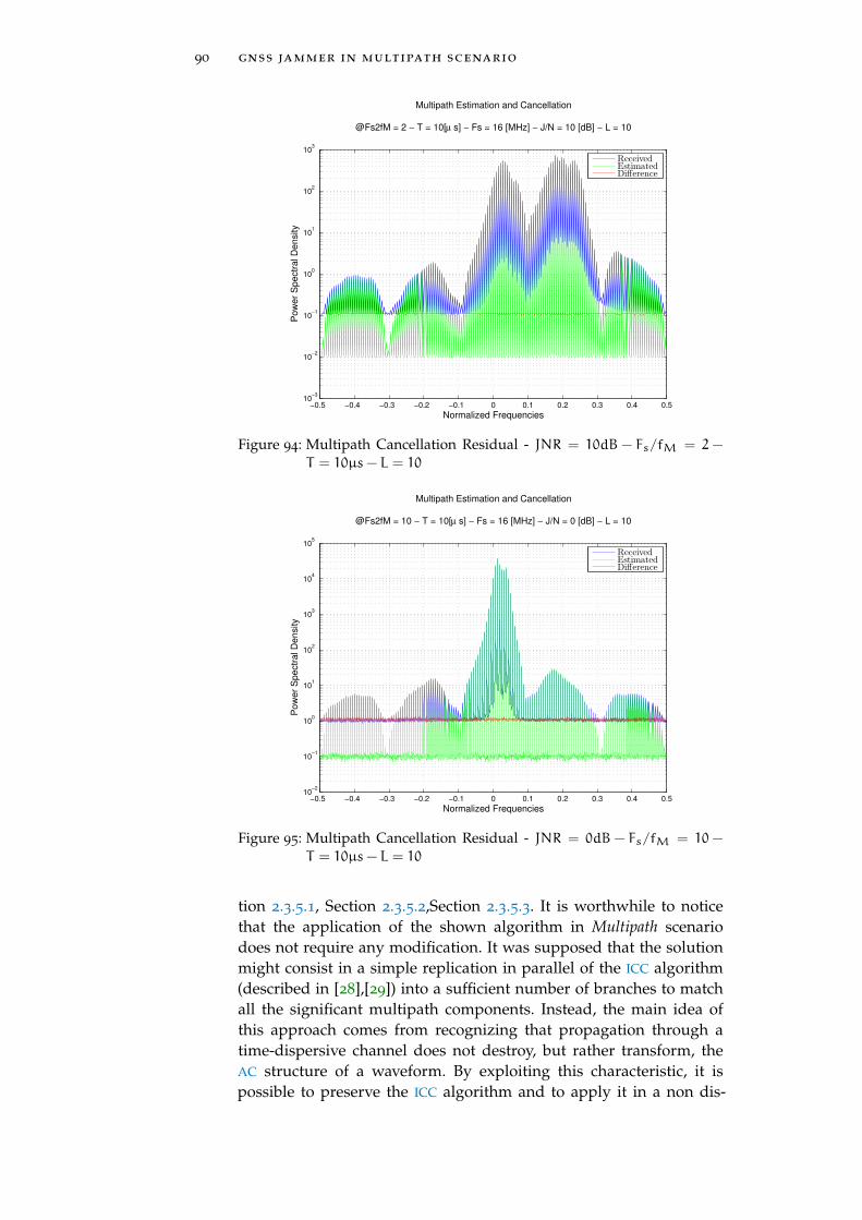
90 gnss jammer in multipath scenario
−0.5 −0.4 −0.3 −0.2 −0.1 0 0.1 0.2 0.3 0.4 0.510
−3
10−2
10−1
100
101
102
103
Multipath Estimation and Cancellation
@Fs2fM = 2 − T = 10[µ s] − Fs = 16 [MHz] − J/N = 10 [dB] − L = 10
Normalized Frequencies
Pow
er
Spect
ral D
ensi
ty
ReceivedEstimatedDifference
Figure 94: Multipath Cancellation Residual - JNR = 10dB − Fs/fM = 2 −
T = 10µs− L = 10
−0.5 −0.4 −0.3 −0.2 −0.1 0 0.1 0.2 0.3 0.4 0.510
−2
10−1
100
101
102
103
104
105
Multipath Estimation and Cancellation
@Fs2fM = 10 − T = 10[µ s] − Fs = 16 [MHz] − J/N = 0 [dB] − L = 10
Normalized Frequencies
Pow
er
Spect
ral D
ensi
ty
ReceivedEstimatedDifference
Figure 95: Multipath Cancellation Residual - JNR = 0dB − Fs/fM = 10 −
T = 10µs− L = 10
tion 2.3.5.1, Section 2.3.5.2,Section 2.3.5.3. It is worthwhile to noticethat the application of the shown algorithm in Multipath scenariodoes not require any modification. It was supposed that the solutionmight consist in a simple replication in parallel of the ICC algorithm(described in [28],[29]) into a sufficient number of branches to matchall the significant multipath components. Instead, the main idea ofthis approach comes from recognizing that propagation through atime-dispersive channel does not destroy, but rather transform, theAC structure of a waveform. By exploiting this characteristic, it ispossible to preserve the ICC algorithm and to apply it in a non dis-
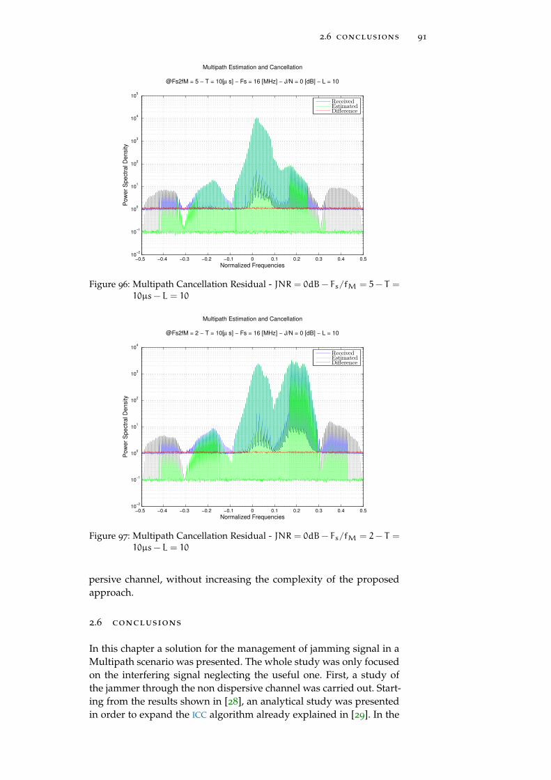
2.6 conclusions 91
−0.5 −0.4 −0.3 −0.2 −0.1 0 0.1 0.2 0.3 0.4 0.510
−2
10−1
100
101
102
103
104
105
Multipath Estimation and Cancellation
@Fs2fM = 5 − T = 10[µ s] − Fs = 16 [MHz] − J/N = 0 [dB] − L = 10
Normalized Frequencies
Pow
er
Spect
ral D
ensi
ty
ReceivedEstimatedDifference
Figure 96: Multipath Cancellation Residual - JNR = 0dB− Fs/fM = 5− T =
10µs− L = 10
−0.5 −0.4 −0.3 −0.2 −0.1 0 0.1 0.2 0.3 0.4 0.510
−2
10−1
100
101
102
103
104
Multipath Estimation and Cancellation
@Fs2fM = 2 − T = 10[µ s] − Fs = 16 [MHz] − J/N = 0 [dB] − L = 10
Normalized Frequencies
Pow
er
Spect
ral D
ensi
ty
ReceivedEstimatedDifference
Figure 97: Multipath Cancellation Residual - JNR = 0dB− Fs/fM = 2− T =
10µs− L = 10
persive channel, without increasing the complexity of the proposedapproach.
2.6 conclusions
In this chapter a solution for the management of jamming signal in aMultipath scenario was presented. The whole study was only focusedon the interfering signal neglecting the useful one. First, a study ofthe jammer through the non dispersive channel was carried out. Start-ing from the results shown in [28], an analytical study was presentedin order to expand the ICC algorithm already explained in [29]. In the
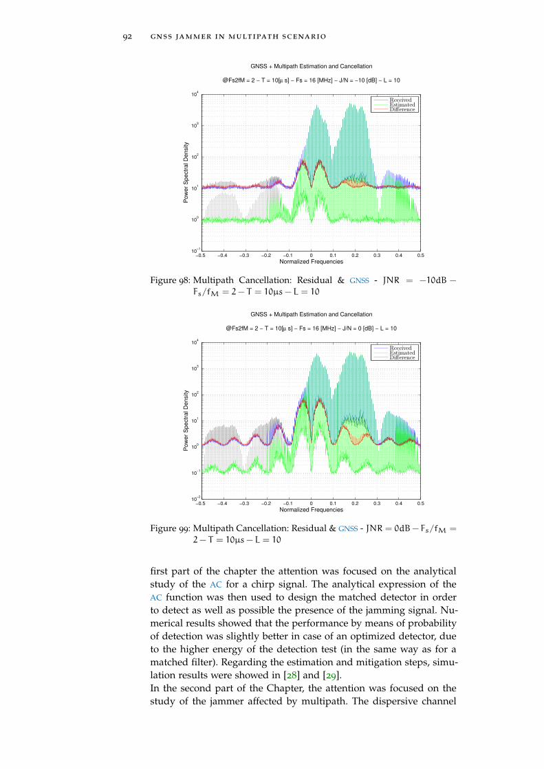
92 gnss jammer in multipath scenario
−0.5 −0.4 −0.3 −0.2 −0.1 0 0.1 0.2 0.3 0.4 0.510
−1
100
101
102
103
104
GNSS + Multipath Estimation and Cancellation
@Fs2fM = 2 − T = 10[µ s] − Fs = 16 [MHz] − J/N = −10 [dB] − L = 10
Normalized Frequencies
Pow
er
Spect
ral D
ensi
ty
ReceivedEstimatedDifference
Figure 98: Multipath Cancellation: Residual & GNSS - JNR = −10dB −
Fs/fM = 2− T = 10µs− L = 10
−0.5 −0.4 −0.3 −0.2 −0.1 0 0.1 0.2 0.3 0.4 0.510
−2
10−1
100
101
102
103
104
GNSS + Multipath Estimation and Cancellation
@Fs2fM = 2 − T = 10[µ s] − Fs = 16 [MHz] − J/N = 0 [dB] − L = 10
Normalized Frequencies
Pow
er
Spect
ral D
ensi
ty
ReceivedEstimatedDifference
Figure 99: Multipath Cancellation: Residual & GNSS - JNR = 0dB− Fs/fM =
2− T = 10µs− L = 10
first part of the chapter the attention was focused on the analyticalstudy of the AC for a chirp signal. The analytical expression of theAC function was then used to design the matched detector in orderto detect as well as possible the presence of the jamming signal. Nu-merical results showed that the performance by means of probabilityof detection was slightly better in case of an optimized detector, dueto the higher energy of the detection test (in the same way as for amatched filter). Regarding the estimation and mitigation steps, simu-lation results were showed in [28] and [29].In the second part of the Chapter, the attention was focused on thestudy of the jammer affected by multipath. The dispersive channel
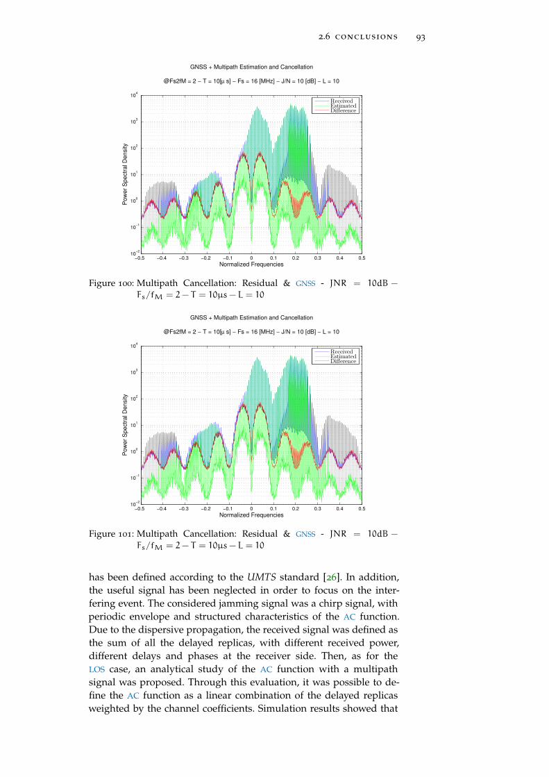
2.6 conclusions 93
−0.5 −0.4 −0.3 −0.2 −0.1 0 0.1 0.2 0.3 0.4 0.510
−2
10−1
100
101
102
103
104
GNSS + Multipath Estimation and Cancellation
@Fs2fM = 2 − T = 10[µ s] − Fs = 16 [MHz] − J/N = 10 [dB] − L = 10
Normalized Frequencies
Pow
er
Spect
ral D
ensi
ty
ReceivedEstimatedDifference
Figure 100: Multipath Cancellation: Residual & GNSS - JNR = 10dB −
Fs/fM = 2− T = 10µs− L = 10
−0.5 −0.4 −0.3 −0.2 −0.1 0 0.1 0.2 0.3 0.4 0.510
−2
10−1
100
101
102
103
104
GNSS + Multipath Estimation and Cancellation
@Fs2fM = 2 − T = 10[µ s] − Fs = 16 [MHz] − J/N = 10 [dB] − L = 10
Normalized Frequencies
Pow
er
Spect
ral D
ensi
ty
ReceivedEstimatedDifference
Figure 101: Multipath Cancellation: Residual & GNSS - JNR = 10dB −
Fs/fM = 2− T = 10µs− L = 10
has been defined according to the UMTS standard [26]. In addition,the useful signal has been neglected in order to focus on the inter-fering event. The considered jamming signal was a chirp signal, withperiodic envelope and structured characteristics of the AC function.Due to the dispersive propagation, the received signal was defined asthe sum of all the delayed replicas, with different received power,different delays and phases at the receiver side. Then, as for theLOS case, an analytical study of the AC function with a multipathsignal was proposed. Through this evaluation, it was possible to de-fine the AC function as a linear combination of the delayed replicasweighted by the channel coefficients. Simulation results showed that
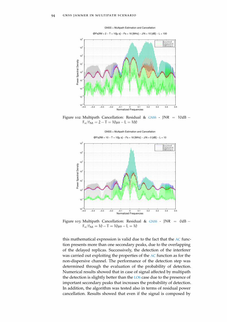
94 gnss jammer in multipath scenario
−0.5 −0.4 −0.3 −0.2 −0.1 0 0.1 0.2 0.3 0.4 0.510
−4
10−3
10−2
10−1
100
101
102
103
104
GNSS + Multipath Estimation and Cancellation
@Fs2fM = 2 − T = 10[µ s] − Fs = 16 [MHz] − J/N = 10 [dB] − L = 100
Normalized Frequencies
Pow
er
Spect
ral D
ensi
ty
ReceivedEstimatedDifference
Figure 102: Multipath Cancellation: Residual & GNSS - JNR = 10dB −
Fs/fM = 2− T = 10µs− L = 100
−0.5 −0.4 −0.3 −0.2 −0.1 0 0.1 0.2 0.3 0.4 0.510
−2
10−1
100
101
102
103
104
105
GNSS + Multipath Estimation and Cancellation
@Fs2fM = 10 − T = 10[µ s] − Fs = 16 [MHz] − J/N = 0 [dB] − L = 10
Normalized Frequencies
Pow
er
Spect
ral D
ensi
ty
ReceivedEstimatedDifference
Figure 103: Multipath Cancellation: Residual & GNSS - JNR = 0dB −
Fs/fM = 10− T = 10µs− L = 10
this mathematical expression is valid due to the fact that the AC func-tion presents more than one secondary peaks, due to the overlappingof the delayed replicas. Successively, the detection of the interfererwas carried out exploiting the properties of the AC function as for thenon-dispersive channel. The performance of the detection step wasdetermined through the evaluation of the probability of detection.Numerical results showed that in case of signal affected by multipaththe detection is slightly better than the LOS case due to the presence ofimportant secondary peaks that increases the probability of detection.In addition, the algorithm was tested also in terms of residual powercancellation. Results showed that even if the signal is composed by
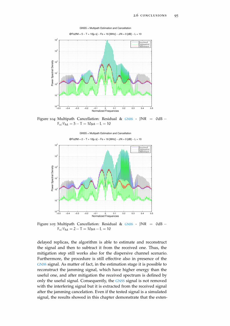
2.6 conclusions 95
−0.5 −0.4 −0.3 −0.2 −0.1 0 0.1 0.2 0.3 0.4 0.510
−2
10−1
100
101
102
103
104
GNSS + Multipath Estimation and Cancellation
@Fs2fM = 5 − T = 10[µ s] − Fs = 16 [MHz] − J/N = 0 [dB] − L = 10
Normalized Frequencies
Pow
er
Spect
ral D
ensi
ty
ReceivedEstimatedDifference
Figure 104: Multipath Cancellation: Residual & GNSS - JNR = 0dB −
Fs/fM = 5− T = 10µs− L = 10
−0.5 −0.4 −0.3 −0.2 −0.1 0 0.1 0.2 0.3 0.4 0.510
−2
10−1
100
101
102
103
104
GNSS + Multipath Estimation and Cancellation
@Fs2fM = 2 − T = 10[µ s] − Fs = 16 [MHz] − J/N = 0 [dB] − L = 10
Normalized Frequencies
Pow
er
Spect
ral D
ensi
ty
ReceivedEstimatedDifference
Figure 105: Multipath Cancellation: Residual & GNSS - JNR = 0dB −
Fs/fM = 2− T = 10µs− L = 10
delayed replicas, the algorithm is able to estimate and reconstructthe signal and then to subtract it from the received one. Thus, themitigation step still works also for the dispersive channel scenario.Furthermore, the procedure is still effective also in presence of theGNSS signal. As matter of fact, in the estimation stage it is possible toreconstruct the jamming signal, which have higher energy than theuseful one, and after mitigation the received spectrum is defined byonly the useful signal. Consequently, the GNSS signal is not removedwith the interfering signal but it is extracted from the received signalafter the jamming cancelation. Even if the tested signal is a simulatedsignal, the results showed in this chapter demonstrate that the exten-
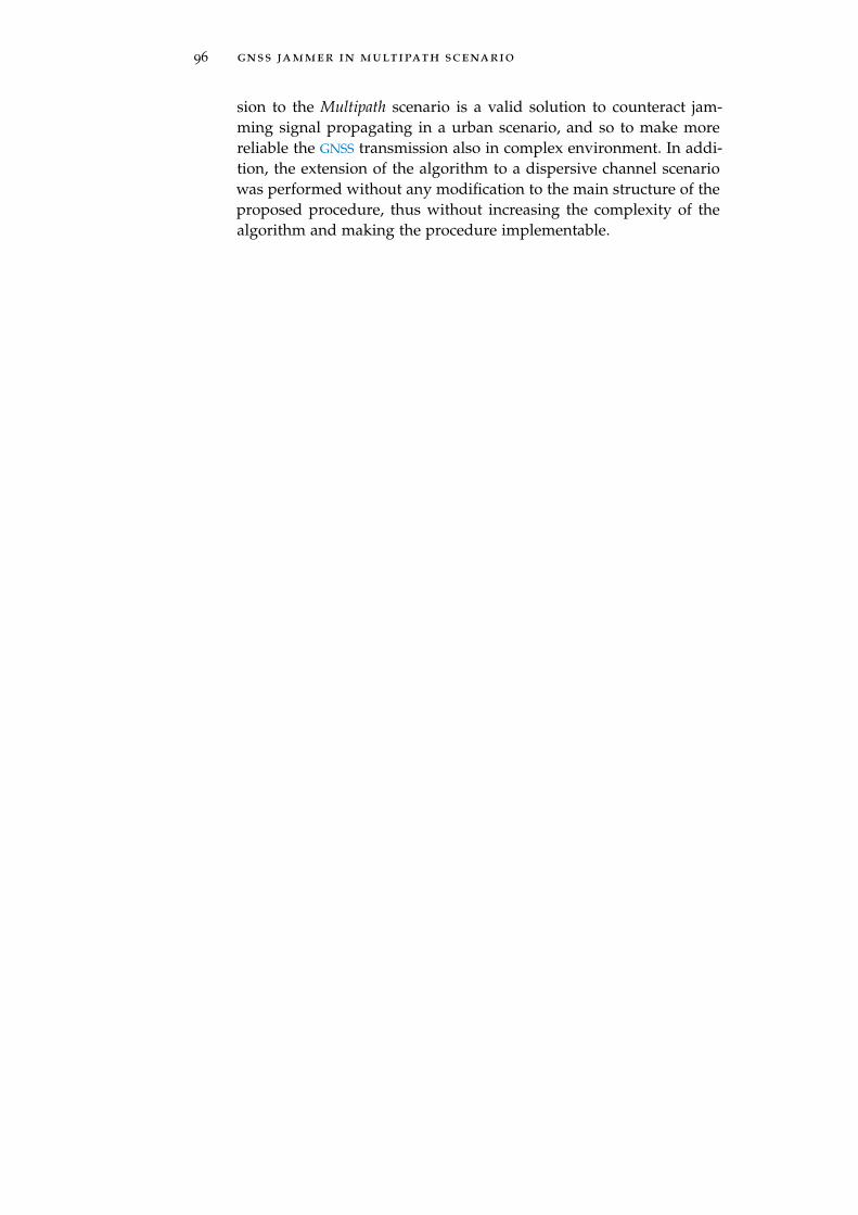
96 gnss jammer in multipath scenario
sion to the Multipath scenario is a valid solution to counteract jam-ming signal propagating in a urban scenario, and so to make morereliable the GNSS transmission also in complex environment. In addi-tion, the extension of the algorithm to a dispersive channel scenariowas performed without any modification to the main structure of theproposed procedure, thus without increasing the complexity of thealgorithm and making the procedure implementable.
I N T E R F E R E N C E M A N A G E M E N T T E C H N I Q U E S :F U RT H E R D E V E L O P M E N T S
It is well known that interference in GNSS is still an open challenge. Inthe previous chapters some approaches have been described. In thefinal chapter it has been shown that it is also possible to mitigate ajamming in worse scenario, introducing a possible research directionin the future developments.
Even if several literature works have been proposed and severaltechniques deeply investigated, improvements can be carried out. Inthis part I detection and mitigation techniques have been described.It has been shown that lower is the signal power, more difficult is thedetection and consequently the mitigation, as expected. The wholestudy has been focused on the statistical characterization of the jam-ming event neglecting the useful GNSS signal. For this reason, theprovided approach has been evaluated for lower power level of theinterfering signal, even if the impact on the useful signal is not effec-tive.
In addition, the mitigation step is still an open topic. In the secondpart of the second chapter it has been demonstrated that jammingsignal can be mitigated also when affected by multipath propagation.The used method exploits the periodic characteristic of the interfer-ing signal. The obtained results are an useful start for further devel-opments in this direction. In particular, the attention will be focusedon the increasing problem represented by the spoofing signal that ismore complex than the previous jamming signals, considered in thedescribed results.
Due to this, efficient anti-jamming and anti-spoofing techniqueswill be needed in order to counteract with more sophisticated distur-bances and guarantee the reliability of the GNSS infrastructure.
97

Part II
S P O O F I N G T H R E AT
Spoofing is notoriously classified as the most dangerousthreat of the GNSS infrastructure. Its main goal is to mis-lead the receiver tracking it and sending wrong informa-tion about its position. The receiver is not conscious of thisattack, and it acquires the counterfeit signal and discardsthe authentic one. The rapid diffusion of GNSS location-based applications in a large set of human activities makesthe navigation system infrastructure very vulnerable againstmalicious attacks which aim to disrupt the functionalitiesfor illegal purposes. Taking into account this scenario, ef-ficient and computationally efficient detection and mitiga-tion techniques are required in order to counteract spoof-ing signals.
The aim of this part II is to present possible and simple ap-proaches in the spoofing detection field. Scenarios affectedby spoofing signals are considered and detection methodsare described pointing out the principal steps and possibleapplications, without neglecting drawbacks.

3S P O O F I N G I N G N S S
3.1 introduction
The easy accessibility to the GNSS signal combined with a non securityfeature, as a cryptographic signature, in the signal modulation anddata streams, makes civil infrastructures using open GNSS stronglyvulnerable to jamming and spoofing attacks due to the predictabilityof open GNSS signals. RFI is considered as the most disruptive eventfor the GNSS system. As reported in [45][11], RFI affects the opera-tion of the AGC and Low Noise Amplifier (LNA) in the RF front-endand it can also deny the correct functions of carrier an code track-ing loops [14][10], causing deterioration and loss of lock in signalreception [36][76]. Thus, due to the high possibility of such attacks,the GNSS security is a very important topic and consequently inten-tional interfering attacks are a serious threat for the overall navigationsystem, considering the rife diffusion in the daily human life appli-cations as emergency and safety-of-life ones 1. In [74] and [78] anexhaustive evaluation of the spoofing threat in civil GPS infrastruc-ture is provided. However, the attention is focused on the increasingrisk of successful spoofing attacks due to the easy accessibility andcheap costs of the hardware and software equipment. Accordingly, itis possible to trick a receiver transmitting a counterfeit signal withfalse estimates of PVT solutions, without any awareness due to the in-trinsic reliability on the receiver output. If an attack is successful thenavigation solutions are not reliable and the consequences are obvi-ous, as misleading the navigation receiver. The aforementioned prob-lem is debated within the chapter analyzing the effects on the GPS L1
frequency signal, considerations that can be extended to other typesof signals an navigation systems. Interference is a difficult threat forthe GNSS infrastructure, and different type of jamming signal can beidentified. Among them, the major issue is represented by the GNSS-like signals as meaconing and spoofing, as well. The former is themost simplistic way to generate a satellite navigation signal. In or-der to define a meaconing attack, it is necessary to have a passiveantenna which receives the useful signal, then an amplifier and atransmission antenna which works at the same GPS frequency of theuseful signal. All the receivers close to the jamming source detectthe broadcast signal and decode the previous antenna position andnot their own. It is possible to detect the presence of a meaconingattack if the rebroadcast signal has a higher power than the origi-nal signal. The latter instead is more sophisticated. It can be madeby a GPS generator and then it is broadcast. In [36] a sophisticatedcase is provided. The spoofer was located close to the GPS receiver
1 Described in: [36][74][67][68][69][79][46][38] [34][35][78]
101
102 spoofing in gnss
in order to acquire the signal characteristics. Successively, the jam-mer was able to reproduce the signal and by slowly increasing itsown transmitting power it captured the target receiver that trackedthe counterfeit signal, thus decoding wrong PVT solutions. Authorsshowed that spoofing goes beyond the aim of denying the correctcommunications between transmitter and receiver, but its own aimis to mislead the target receiver sending incorrect position and timeinformation. In this chapter possible approaches to counteract spoof-ing events are discussed. Taking into account all the results providedin [4], we proposed possible improvements exploiting AGC propertiesjointly to other metric measurements of the GPS receiver. The follow-ing sections will present a survey of the previous approaches andcountermeasures in RFI and spoofing detection with particular atten-tion on Signal Quality Monitoring (SQM) and AGC-based techniques.First, a brief introduction of the existing techniques is provided inSection 3.2. In Section 3.3 a well referred to SQM approaches reviewis reported. Successively, in Section 3.4 the concept of the AGC is de-scribed also in its application as a spoofer detection combined withthe correlator and C/N0 measurements. Numerical results have beencarried out studying and extracting information from collected dataand they are showed in Section 3.5 in order to validate our approach.Finally, in Section 3.6 conclusions are provided with possible improve-ments.
3.2 literature survey
At the beginning of GPS working system, several studies showed thatthe the recent systems could be susceptible to intentional jammingattacks. The countermeasure was to introduce a Y-code componentto the military P-code signal in order to guarantee a reliable and ef-fective transmission [37][75]. Apparently, these methods was recog-nized as a powerful technique in order to limit and avoid spoofingattacks. The drawback was that researchers did not take into accountthe possibility of spoofing attacks in civil infrastructure [60][57],[50].This method assumed that the encrypted P(Y)-code is free of spoof-ing, and a reference receiver set at a safe location that is not subject tospoofing. The user receiver is the possible spoofing victim. Statistic ofcross correlation between two receivers allows detecting the spoofingat a victim receiver. Although, it requires a secure communicationslink and a second receiver in order to exploit correlation propertiesit is still one of the more effective low computational methodologiesproposed to date and it leverages the existing military signals.
Furthermore, it could be possible to design civil signal waveformwhich have intrinsic anti-spoofing capabilities. These have been inves-tigated and candidates proposed [66]. In any case, the signal designcycle is extremely long and it requires modifications in GNSS infras-tructure, so it is hard to implement these new waveforms in the nearfuture.
3.2 literature survey 103
A possible detection approach is defined by observing the behaviorof the user’s position or time estimates, usually for less sophisticatedjamming attacks. If an unrealistic time-position jump occurs, as deter-mined by the navigation Kalman filter, this could be used as flag ofspoofing event. Several examples have been presented in [62][77].
Similarly, Receive Autonomous Integrity Monitoring (RAIM) tech-niques are able to detect malicious events. These techniques can beemployed at position solution level and they are quite effective for theless sophisticated attacks. These methods are not computationally ex-pensive though the single epoch mechanism for detection is quite sen-sitive to the jump magnitude-filter tuning. However, RAIM techniqueswork very well only if few spoofing events occur among several au-thentic solutions. On the other hand, if the majority of the signals arespoofed RAIM techniques discard the authentic signal, cause the maingoal is to minimize the residual among received solutions.
In case of a single GPS antenna, detection can be performed lever-aging a well-known technique based on adding inertial sensors andalso cross checking the consistency of dynamics [82][47]. This methodtests a residual between GPS spoofed measurements and inertial mea-surements, and monitors their discrepancies. Due to the availabilityand low cost of multi-axis MEMS accelerometers, the implementationof these techniques should be quite effective to consider and cross-compare reported movement, raising a confidence flag when they donot agree. However, the majority of common GPS receivers do nothave such sensors. Furthermore, low cost inertial sensors are effectiveonly in a short space of operating time under continuous spoofingenvironments, besides high-end sensors are more expensive than GPS
receivers.Spoofing detection and mitigation techniques could be defined mod-
ifying the pattern of the receiver’s antenna. The GPS antenna is eitheromnidirectional (mobile devices) or hemispherical (fixed locations)and receives signals from all directions. A multi-antenna receiver canimplement array techniques to steer beams toward the known direc-tion of the satellites and nulls toward interfering power sources. Thus,the antenna array is one of the few methods that can both flag andattempt to mitigate a potential spoofing event when it occurs. Re-searchers have also proposed a synthetic array, applicable for a singleantenna dynamic receiver, which is able to determine the presenceof a spoofing source. It is functional but it has the drawback of in-creasing complexity and it is only applicable for a single stationaryspoofing source [56][20].
The major limitation of spoofing is how it transmits the counterfeitGNSS signals. The fake signals are transmitted by the same wirelesschannel and they have the same propagation characteristics, regard-less if the GNSS receiver is moving or not. A signal spatial correlationtest was conducted to detect the spoofing [17]. The counterfeit sig-nals are spatially correlated even if the GNSS antenna receiver is mov-ing along an arbitrary trajectory. The detection technique was basedon the monitoring of amplitude and Doppler correlation between all(fake and authentic) tracked signals. The presence of a spoofing at-
104 spoofing in gnss
tack is defined when a pairwise correlation is evaluated. However,it is worth to notice that this method was carried out in a scenariowhere multipath fading was absent and considering a fixed/station-ary spoofing source.
Another possible technique consists in observing the channel com-ponents of the tracked signals. In [5] the described detection tech-nique is based on the analysis of multipath components that affectGNSS signals propagation. A spoofing signal could be considered as adelayed replica of the authentic GNSS signal. The fundamental aspectis to observe the behavior in term of amplitude, delay and phase com-ponent of all the tracked paths. In case of a spoofing event these threeparameters have different time envelope with respect to the multi-path reflection. For example if the delay increases but the amplitudedoes not decrease as expected, according to the rules of multipathpropagation, the presence of spoofing could be determined. A pre-despreading detection technique is presented in [42]. It consists inobserving GNSS signal features in order to assess the presence of aspoofing signal before the de-spreading stage of the GNSS receiver.This technique operates on raw samples data looking at the abnormalbehavior of the signal power content of the GPS spectrum. In this waya counterfeit event could be detected in the digital domain, exploit-ing the Delay and Multiply (DAM) property of the GPS code whenthe spoofing event has enough power to interrupt normal receiver’soperation. In [44] a spoofing detection and protection technique isdescribed. This method consists in statistical tests of Doppler, C/N0
and PVT solutions and relies on the information that the receiver ob-tained before the suspected spoofing attack. All these steps are per-formed by an independent module in the receiver operation chainthat is able to keep memory of the GNSS signal’s statistics. The pro-posed tests are based on monitoring the variance of Doppler offsetand C/N0 which change with the presence of spoofing, defining dis-tortion in the metrics. Once the spoofing is detected, the receiver usesstored information to start the correct acquisition procedure. How-ever, this solution requires a complex processing unit inside the GNSS
tracking chain with consequently computational costs. Moreover, sev-eral attempts for detection of GNSS spoofing events, even the mostsophisticated ones, have been done in the signal processing domain.Most of them exploit correlation measurement and apply SQM tech-niques. The scope is to find, if present, additional correlation peaksthat can show a possible spoofing attack [81][73][55]. Unfortunately,in order to have an updated correlator measurement, the computa-tional complexity of the receiver has to be increase. Even if this couldbe possible, the next challenge is being able to discern between spoof-ing attack and multipath propagation effects.An exhaustive review of the spoofing detection methods is providedin [43].
3.3 spoofing detection : signal quality monitoring techniques 105
3.3 spoofing detection : signal quality monitoring tech-niques
Monitoring and detecting anomalies and disturbances on receivedsignals are important steps to assess that receiver could be affected bya counterfeit signal. In order to have reliable positioning and naviga-tion solutions, it is necessary to monitor the quality of the broadcastGPS signals. Several methods to detect anomalies by observing PVT
solutions or processing received data have been investigated. Amongthese methods, SQM is the rising one. It is based on observing thebehavior on time of the correlation shape by comparing outputs witha well-defined metric: the most common SQM tests are the Delta andRatio tests, designed to identify asymmetric correlation peaks and toidentify abnormal shape of the correlation peaks, respectively [59]. Inprevious literature, SQM techniques have been proposed as a methodto monitor in time the envelope of the correlation function in mul-tipath scenarios [27]. In the tracking stage the effects of a possiblespoofing event are very similar to multipath ones: distortions of thecorrelation outputs due to the spoofing attack could be assessed asa strong multipath which is in-phase with the authentic signal. Thus,the SQM method has been extended for detection of spoofing attacks.In [19] authors have implemented the Ratio Test metric, proposedin [27], to detect any asymmetry and distortion in the correlation out-puts due to an intermediate spoofing attack. They have observed bothcode and carrier tracking stages: the alignment of the fake signal incode-phase and carrier domains determines not suitable outputs fromDelay Lock Loop (DLL) and Phase-Locked Loop (PLL). In [49] authorshave analyzed two cases of intermediate spoofing attack. Firstly, thespoofer has to align its counterfeit signal to the authentic one, andpossibly (once aligned) it has to increase the power on order to betracked. This kind of spoofer is able to reach the code-phase align-ment with the authentic GPS signal, that could be in constructive ornot constructive interference. It was showed that the delta and ratiotest are not able to detect the spoofing event if this is in constructiveinterference with the real signal. On the other hand, when the fakesignal is out of phase with the authentic one Delta and Ratio test dis-criminators have different values from the nominal case, i.e. when thespoofer is not detected. However, it is necessary that the attack is notrapid in order to detect the presence of the spoofer. Thus, it could beassessed that SQM antispoofing techniques are valid methods to detectthe counterfeit event with the assumption that the receiver alreadytracked the authentic signal. However, these methods could presentsome issues in a multipath propagation scenario because they couldnot distinguish between spoofing attack and a delayed reflection, sothe detection flag will be raised if one of these occurs. For this reason,the implementation of a joint metric detection technique is needed.In [6] authors have proposed to use extra correlators jointly with theRatio Test metric in order to overcome the ambiguity problem in de-tecting spoofer or multipath event. An important step is to define thesetting of the correlator and extra-correlator, in order to detect vesti-
106 spoofing in gnss
gial signal presence. It is necessary that the two implemented metricscan be effective in the same portion of code delay. On the contrary,they will share only a small part and the detection results will benot reliable. In addition, it is possible that the effects of counterfeitsignal could not be present in both metrics during the same time ofobservation. Thus, it is necessary to extend the observation time anda parallel check in both metrics is required: if both metrics presenta high probability of detection, the receiver is able to distinguish be-tween spoofer and multipath events. However, this joint detectiontechniques is not reliable with a high power spoofing signal. Thestrong counterfeit signal hides the real signal under the noise floorand the receiver is not able to understand that the tracked signal is thefake one: Ratio Test does not detect any distortion in the correlationfunction shape. Another joint detection technique has been proposedin [80]. The authors have described a non-cryptographic method forspoofing detection that consists in implementing jointly a correlationfunction distortion monitor and a total in-band power monitor. Thistechnique relies on the incapability of a spoofer device to maintain forlong time a low-power attack in order to not cause abnormal shape inthe receiver correlator outputs. These two independent metrics con-sist in a symmetric difference between an early-late correlator pair(non-normalized Delta Test) and the measure of the total power inreceiver bandwidth. The first metric aims to detect distortions in thecorrelation shape. The reliability of this result depends on the choiceof the time-offset between the early and late local replica. The powermonitor metric aims to measure the nominal value of the in-bandpower and to detect anomalies in increasing power when a spoofingevent occurs.In conclusion, many literature works state that SQM techniques are ef-ficient spoofing detection solutions in a LOS scenario. However, withdistorted propagation channel, i. e.the signal is affected by multipathand/or huge atmospheric interferences, the aforementioned techniquesare not able to perfectly distinguish the presence or absence of thespoofing event.
3.4 proposed architecture
In the previous sections, literature reviews for detection spoofing tech-niques and in particular for SQM approaches have been described. Itis well known that the structure of the spoofing signal is GNSS-like,because it is generated in order to tick and mislead the target re-ceiver. However, so that the attack to be effective, spoofing source hasto reproduce and broadcast at least four Pseudorandom Noise (PRN)signals. And if an attack occurs, the detection is still difficult in partic-ular before the de-spreading step. Some methods have been alreadypresented, as the constant monitoring of the AGC response in orderto measure unexpected values [4]. The provided method is very ef-fective, but its main drawback consists in requiring enough informa-tion about the AGC component: it is not implementable in GNSS soft-
3.4 proposed architecture 107
ware receiver because it is not working with digital domain samples.Moving from these considerations, a method that consists in the jointobservation of measurement outputs from different components ofthe GNSS receiver is proposed. The main goal is to provide a possi-ble detection technique based on the observation of the AGC signalwaveform aided with the information carried out from the correla-tion function and from the estimation of the C/N0. For this purpose,firstly a description of the scenario is provided followed by the intro-duction to each metric used to detect the jamming threat.
3.4.1 System model
In [43] a simplistic expression of a spoofing signal is defined. As al-ready said, the spoofing source generates many counterfeit PRNs thathave quite the same power level of the authentic ones, a bit higher inorder to attract the target to be spoofed. The spoofed received signalis written as [43]:
r(nTs) =
M∑m=1
√pamh
am (nTs − τ
am) cam (nTs − τ
am) ejφ
am+j2πfamnTs (83)
+
N∑q=1
√psqh
sq
(nTs − τ
sq
)csq(nTs − τ
sq
)ejφ
sq+j2πf
sqnTs + η (nTs)
where Ts is the sampling interval, φ is the carrier phase, f is theDoppler frequency, p is the signal power and τ is the code delay;the subscripts m and q (and the upscripts a and s) correspond toauthentic and spoofed PRN signal, respectively. The symbol h(nTs)represents the transmitted data the and c(nTs) is the PRN sequence,M is the total number of authentic and N of spoofed received signals;η(nTs) is the complex AWGN with zero-mean and variance equal to σ2.According to the value of spoofed PRNs it is possible to differentiatethe type of the spoofing attack. However, the spoofing source has togenerate signal with a very similar power to the authentic ones, andconsequently the received power level increases due to the jammingcontributions [43].
3.4.2 Automatic Gain Control
The AGC adjusts the power level of the intermediate frequency signalat Analog-to-Digital Converter (ADC) input in order to minimize thequantization loss. The presence of the AGC is necessary to calibratethe gain in order to define a correct received input power. It is wellknow that the GNSS signal power at the Earth’s surface is below thethermal noise floor, which is expressed as:
PN = kTABW (84)
where k is the Boltzmann’s constant, TA is the antenna temperatureand BW is the bandwidth. The thermal noise is then added to the
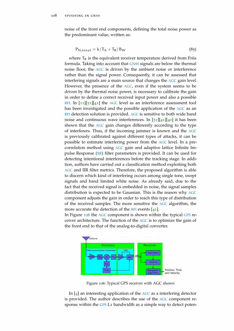
108 spoofing in gnss
noise of the front end components, defining the total noise power asthe predominant value, written as:
PN,total = k (TA + TR)BW (85)
where TR is the equivalent receiver temperature derived from Friisformula. Taking into account that GNSS signals are below the thermalnoise floor, the AGC is driven by the ambient noise or interferencerather than the signal power. Consequently, it can be assessed thatinterfering signals are a main source that changes the AGC gain level.However, the presence of the AGC, even if the system seems to bedriven by the thermal noise power, is necessary to calibrate the gainin order to define a correct received input power and also a possibleRFI. In [11][51][41] the AGC level as an interference assessment toolhas been investigated and the possible application of the AGC as anRFI detection solution is provided. AGC is sensitive to both wide bandnoise and continuous wave interferences. In [51][41][40] it has beenshown that the AGC gain changes differently according to the typeof interferers. Thus, if the incoming jammer is known and the AGC
is previously calibrated against different types of attacks, it can bepossible to estimate interfering power from the AGC level. In a pre-correlation method using AGC gain and adaptive lattice Infinite Im-pulse Response (IIR) filter parameters is provided. It can be used fordetecting intentional interferences before the tracking stage. In addi-tion, authors have carried out a classification method exploiting bothAGC and IIR filter metrics. Therefore, the proposed algorithm is ableto discern which kind of interfering occurs among single tone, sweptsignals and band limited white noise. As already said, due to thefact that the received signal is embedded in noise, the signal samplesdistribution is expected to be Gaussian. This is the reason why AGC
component adjusts the gain in order to reach this type of distributionof the received samples. The more sensitive the AGC algorithm, themore accurate the detection of the RFI events [41].In Figure 106 the AGC component is shown within the typical GPS re-ceiver architecture. The function of the AGC is to optimize the gain ofthe front end to that of the analog-to-digital converter.
Figure 106: Typical GPS receiver with AGC shown
In [4] an interesting application of the AGC as a interfering detectoris provided. The author describes the use of the AGC component re-sponse within the GPS L1 bandwidth as a simple way to detect poten-
3.4 proposed architecture 109
tial spoofing signals. The noise-driven characteristic causes instabilityof the AGC output due to the continuous gain variation according tothe received power. Taking into account this, a calibration of the AGC
is necessary in order to define statistical properties in the nominalconditions, i. e.without spoofing events. The proposed results showthat the presence of the spoofer, after an accurate calibration, addsenergy in the useful band with a consequent drop of the AGC gainlevel. However, all the testing results have been carried out in a con-trolled scenario, neglecting how much jamming events can occur inreal sites. Given that, an AGC-centric approach will not be reliable asit could arise false alarm flag too often. Consequently, the only AGC
component cannot be considered as a stand-alone detector, but it canbe considered as a complement to other approaches, providing aneffective spoofer detection.
3.4.3 Correlator
In order to deny the correct GNSS acquisition and tracking procedures,spoofing signal make a fake correlation peaks being able to overlapthe authentic one, leading the target receiver to a wrong trackingsolution. The correlation output could be distorted by a spoofing at-tack, but the effect of the interaction with the authentic signal can bemistaken for multipath effects. Thus, some of the mitigation of multi-path effect have been used to detect spoofing signals [59][19]. Firstly,the spoofer has to align its counterfeit signal to the authentic one,and possibly once aligned it has to increase the power in order tobe tracked by the receiver tracking loop. In order to be aligned withthe useful signal, spoofing has to perfectly know the position of thetarget receiver and thus estimate correctly necessary parameters. In-stead, when the spoofer is not able to define in a correct manner thesynchronization with the authentic signals, it the correlation windowa strong correlation peak appear. This additional peak moves towardsthe authentic one trying to misdirect the tracking solution.
3.4.4 C/N0 estimation
As for the previous measurements, the carrier-to-noise ratio C/N0
estimation can be used to detect RFI events, but it is a noisy measure-ments. The environmental effects can strongly affect the C/N0 mea-surements, but unlike the AGC information the C/N0 measurementscan be easily obtained from the receiver as it is an observable informa-tion. The C/N0 is a wide used metric in assessment of the quality ofthe tracking signals. This value is always evaluated in function of theelevation angle: greater the elevation angle, the higher the value ofthe C/N0, due to the clear visibility of the satellites in orbits. When aRFI event occurs, consequently there is variation in the estimate C/N0
value. RFI raises the noise floor and thus the C/N0 presents a dropproportional to the interfering power that jams the target receiver. Inpresence of a spoofing signal the effects on the C/N0 estimate are
110 spoofing in gnss
similar to the RFI case. The spoofer can increase the noise floor of thetarget receiver with the aim to disrupt the acquisition and tracking ofthe authentic signals, but conversely to the RFI case the spoofer cre-ates correlation peaks and thus C/N0 value commensurable to theauthentic one. Thus, the detection is more difficult due to the capa-bility of the spoofer source to generate counterfeit PRNs with a powerequivalent to the expected one.
3.4.5 AGC & Correlator & C/N0 : A combined Technique
In the previous sections a brief description of the measurements pro-vided by components inside the GNSS receiver is reported. The proper-ties of the aforementioned approaches have been described, defininghow them can be implemented as a jamming and spoofing detec-tion techniques. The drawback is that all the methods proposed as aself-contained anti-jamming techniques, an thus considered indepen-dently, cannot be implemented due to their high probability of falsealarm. As a matter of fact, for the AGC if a previous calibration isnot made, the spoofing detection by means of the drops on the AGC
level is not reliable, due to the fact that the components is driven bynoise and thus any type of interference can be classified as a spoofingsignal. The correlation distortion measurement can be lead astray bymultipath components and the C/N0 estimates is highly sensitive toany type of events that increases the noise floor in the GNSS receiver.In [80] authors have proposed a non cryptographic GNSS anti-spoofingtechnique which exploits the difficulty of a spoofing source to gener-ate a successful attack with both low PRNs power and minimizing thedistortion in the correlation profile. The described method consists inmonitoring simultaneously the received power and the distortion inthe correlation shape. According to the authors, the combination ofthe two techniques permits to discern between multipath and spoof-ing effect and also to reduce the false-alarm probability with respectto the stand-alone approach.Taking into account all these consideration and possible drawbacksof the aforementioned techniques, we propose a spoofing detectiontechnique that relies on the combined observation and evaluation ofthe measurement carried out by the components of the GNSS receiver,i. e.AGC gain level, correlation shape and C/N0 envelope. As alreadystated, all the measurements are sensitive to the fluctuation due to thepresence of the noise power and taken individually they are not reli-able in detection spoofing effect. However, if a spoofer attack occurs,it determines contemporary distortions in all the processing measure-ment and thus it is possible to define a detection method by observinghow and when these distortions are present. For example, if the AGC
gain level has a very huge drop, the correlation distortion monitorpresents a lack of the expected shape and the C/N0 value is verylow even if the elevation angle is high, this could mean that a highpower jamming event is occurring. Instead, if the AGC gain level hasa fluctuation, the correlation distortion presents a variation without
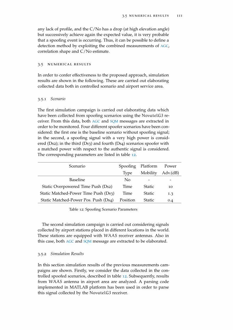
3.5 numerical results 111
any lack of profile, and the C/N0 has a drop (at high elevation angle)but successively achieve again the expected value, it is very probablethat a spoofing event is occurring. Thus, it can be possible to define adetection method by exploiting the combined measurements of AGC,correlation shape and C/N0 estimate.
3.5 numerical results
In order to confer effectiveness to the proposed approach, simulationresults are shown in the following. These are carried out elaboratingcollected data both in controlled scenario and airport service area.
3.5.1 Scenario
The first simulation campaign is carried out elaborating data whichhave been collected from spoofing scenarios using the NovatelG3 re-ceiver. From this data, both AGC and SQM messages are extracted inorder to be monitored. Four different spoofer scenarios have been con-sidered: the first one is the baseline scenario without spoofing signal;in the second, a spoofing signal with a very high power is consid-ered (Ds2); in the third (Ds3) and fourth (Ds4) scenarios spoofer witha matched power with respect to the authentic signal is considered.The corresponding parameters are listed in table 12.
Scenario Spoofing Platform Power
Type Mobility Adv.(dB)
Baseline No - -
Static Overpowered Time Push (Ds2) Time Static 10
Static Matched-Power Time Push (Ds3) Time Static 1.3
Static Matched-Power Pos. Push (Ds4) Position Static 0.4
Table 12: Spoofing Scenario Parameters
The second simulation campaign is carried out considering signalscollected by airport stations placed in different locations in the world.These stations are equipped with WAAS receiver antennas. Also inthis case, both AGC and SQM message are extracted to be elaborated.
3.5.2 Simulation Results
In this section simulation results of the previous measurements cam-paigns are shown. Firstly, we consider the data collected in the con-trolled spoofed scenarios, described in table 12. Subsequently, resultsfrom WAAS antenna in airport area are analyzed. A parsing codeimplemented in MATLAB platform has been used in order to parsethis signal collected by the NovatelG3 receiver.
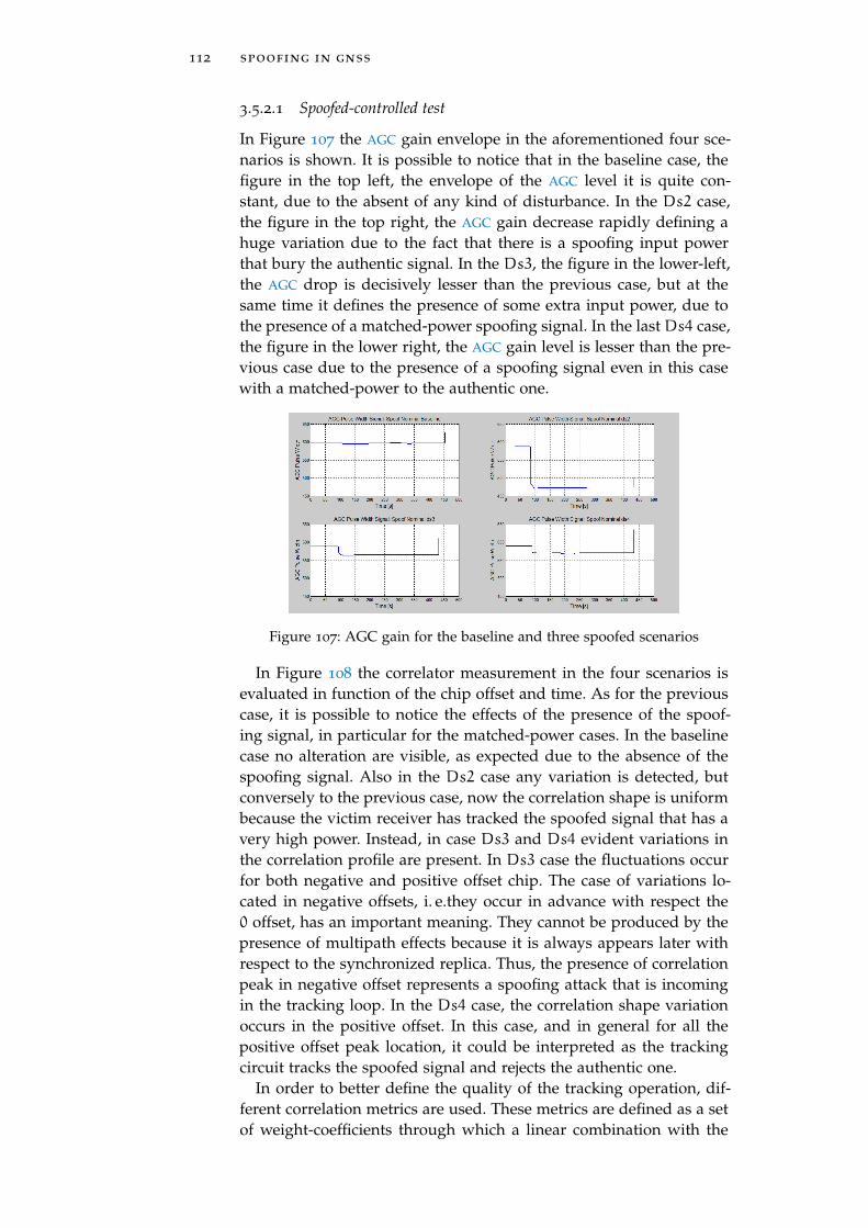
112 spoofing in gnss
3.5.2.1 Spoofed-controlled test
In Figure 107 the AGC gain envelope in the aforementioned four sce-narios is shown. It is possible to notice that in the baseline case, thefigure in the top left, the envelope of the AGC level it is quite con-stant, due to the absent of any kind of disturbance. In the Ds2 case,the figure in the top right, the AGC gain decrease rapidly defining ahuge variation due to the fact that there is a spoofing input powerthat bury the authentic signal. In the Ds3, the figure in the lower-left,the AGC drop is decisively lesser than the previous case, but at thesame time it defines the presence of some extra input power, due tothe presence of a matched-power spoofing signal. In the last Ds4 case,the figure in the lower right, the AGC gain level is lesser than the pre-vious case due to the presence of a spoofing signal even in this casewith a matched-power to the authentic one.
Figure 107: AGC gain for the baseline and three spoofed scenarios
In Figure 108 the correlator measurement in the four scenarios isevaluated in function of the chip offset and time. As for the previouscase, it is possible to notice the effects of the presence of the spoof-ing signal, in particular for the matched-power cases. In the baselinecase no alteration are visible, as expected due to the absence of thespoofing signal. Also in the Ds2 case any variation is detected, butconversely to the previous case, now the correlation shape is uniformbecause the victim receiver has tracked the spoofed signal that has avery high power. Instead, in case Ds3 and Ds4 evident variations inthe correlation profile are present. In Ds3 case the fluctuations occurfor both negative and positive offset chip. The case of variations lo-cated in negative offsets, i. e.they occur in advance with respect the0 offset, has an important meaning. They cannot be produced by thepresence of multipath effects because it is always appears later withrespect to the synchronized replica. Thus, the presence of correlationpeak in negative offset represents a spoofing attack that is incomingin the tracking loop. In the Ds4 case, the correlation shape variationoccurs in the positive offset. In this case, and in general for all thepositive offset peak location, it could be interpreted as the trackingcircuit tracks the spoofed signal and rejects the authentic one.
In order to better define the quality of the tracking operation, dif-ferent correlation metrics are used. These metrics are defined as a setof weight-coefficients through which a linear combination with the
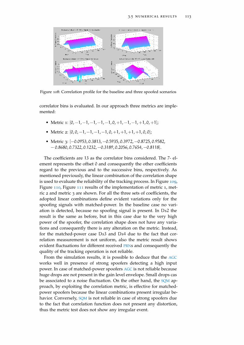
3.5 numerical results 113
Figure 108: Correlation profile for the baseline and three spoofed scenarios
correlator bins is evaluated. In our approach three metrics are imple-mented:
• Metric 1: [0,−1,−1,−1,−1,−1, 0,+1,−1,−1,+1, 0,+1];
• Metric 2: [0, 0,−1,−1,−1,−1, 0,+1,+1,+1,+1, 0, 0];
• Metric 3: [−0.0953, 0.3813,−0.5935, 0.3972,−0.8725, 0.9582,− 0.8680, 0.7322, 0.1232,−0.3189, 0.2056, 0.7654,−0.8118].
The coefficients are 13 as the correlator bins considered. The 7- el-ement represents the offset 0 and consequently the other coefficientsregard to the previous and to the successive bins, respectively. Asmentioned previously, the linear combination of the correlation shapeis used to evaluate the reliability of the tracking process. In Figure 109,Figure 110, Figure 111 results of the implementation of metric 1, met-ric 2 and metric 3 are shown. For all the three sets of coefficients, theadopted linear combinations define evident variations only for thespoofing signals with matched-power. In the baseline case no vari-ation is detected, because no spoofing signal is present. In Ds2 theresult is the same as before, but in this case due to the very highpower of the spoofer, the correlation shape does not have any varia-tions and consequently there is any alteration on the metric. Instead,for the matched-power case Ds3 and Ds4 due to the fact that cor-relation measurement is not uniform, also the metric result showsevident fluctuations for different received PRNs and consequently thequality of the tracking operation is not reliable.
From the simulation results, it is possible to deduce that the AGC
works well in presence of strong spoofers detecting a high inputpower. In case of matched-power spoofers AGC is not reliable becausehuge drops are not present in the gain level envelope. Small drops casbe associated to a noise fluctuation. On the other hand, the SQM ap-proach, by exploiting the correlation metric, is effective for matched-power spoofers because the linear combinations present irregular be-havior. Conversely, SQM is not reliable in case of strong spoofers dueto the fact that correlation function does not present any distortion,thus the metric test does not show any irregular event.
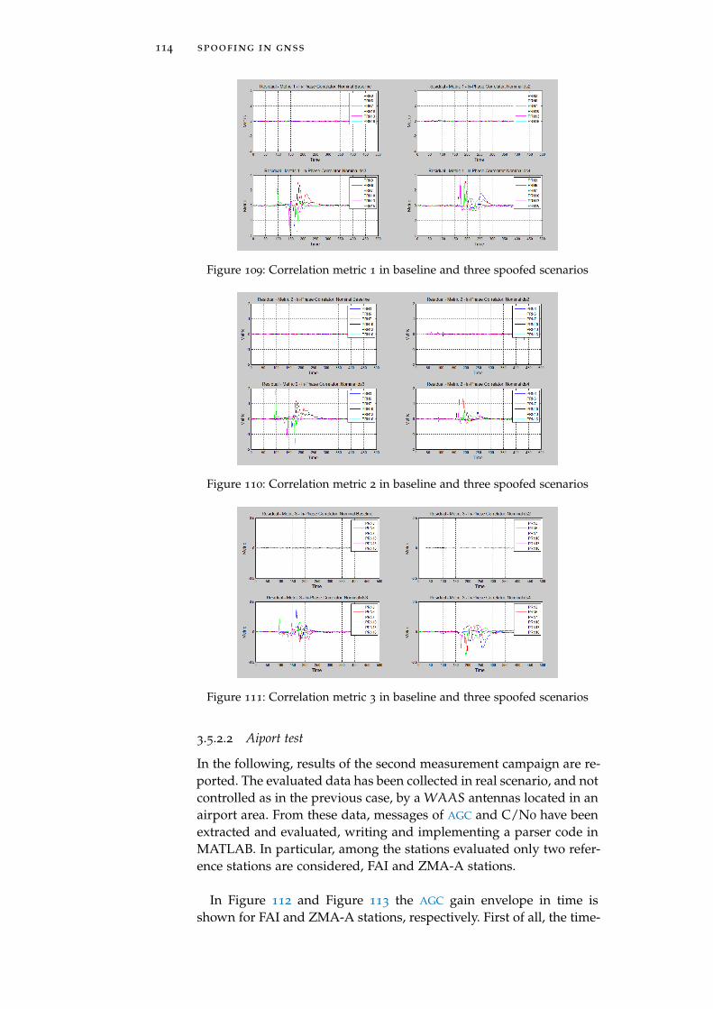
114 spoofing in gnss
Figure 109: Correlation metric 1 in baseline and three spoofed scenarios
Figure 110: Correlation metric 2 in baseline and three spoofed scenarios
Figure 111: Correlation metric 3 in baseline and three spoofed scenarios
3.5.2.2 Aiport test
In the following, results of the second measurement campaign are re-ported. The evaluated data has been collected in real scenario, and notcontrolled as in the previous case, by a WAAS antennas located in anairport area. From these data, messages of AGC and C/N0 have beenextracted and evaluated, writing and implementing a parser code inMATLAB. In particular, among the stations evaluated only two refer-ence stations are considered, FAI and ZMA-A stations.
In Figure 112 and Figure 113 the AGC gain envelope in time isshown for FAI and ZMA-A stations, respectively. First of all, the time-
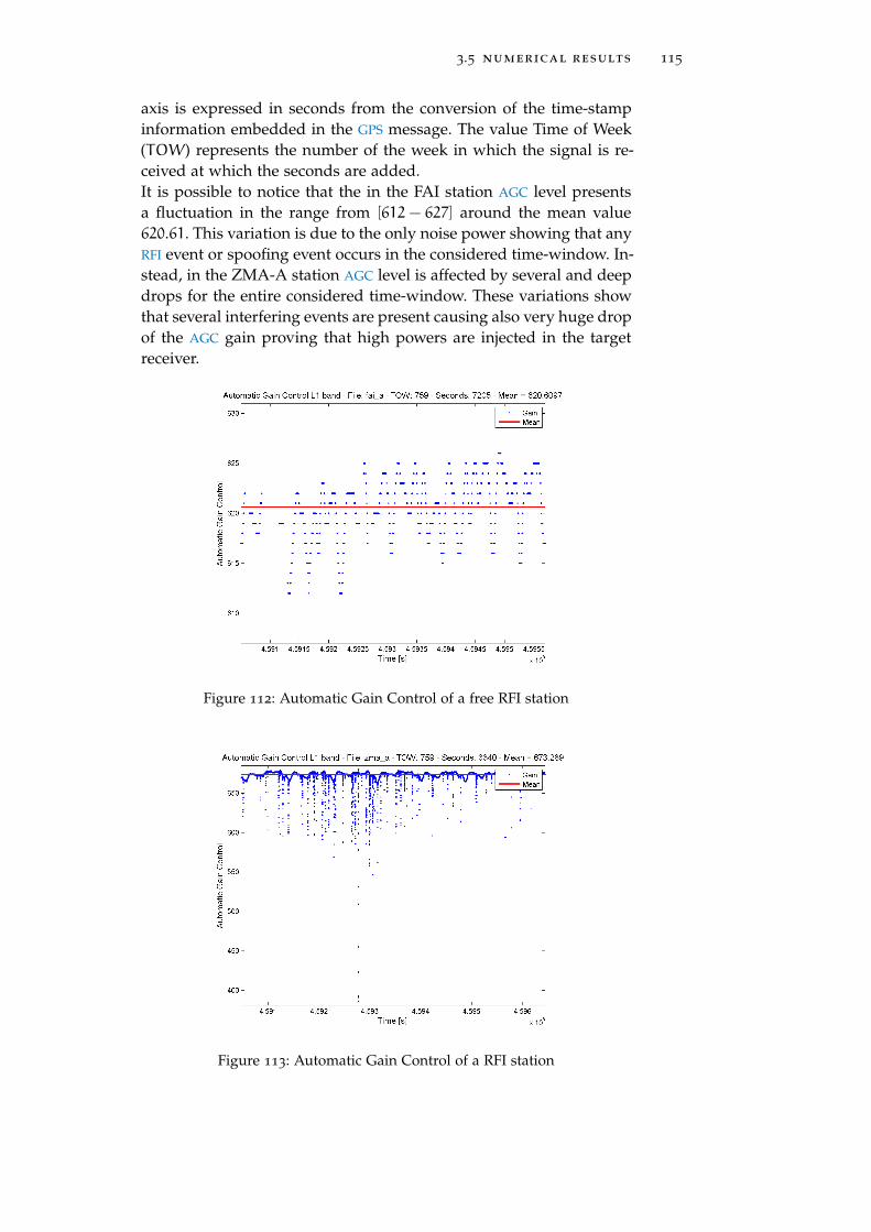
3.5 numerical results 115
axis is expressed in seconds from the conversion of the time-stampinformation embedded in the GPS message. The value Time of Week(TOW) represents the number of the week in which the signal is re-ceived at which the seconds are added.It is possible to notice that the in the FAI station AGC level presentsa fluctuation in the range from [612 − 627] around the mean value620.61. This variation is due to the only noise power showing that anyRFI event or spoofing event occurs in the considered time-window. In-stead, in the ZMA-A station AGC level is affected by several and deepdrops for the entire considered time-window. These variations showthat several interfering events are present causing also very huge dropof the AGC gain proving that high powers are injected in the targetreceiver.
Figure 112: Automatic Gain Control of a free RFI station
Figure 113: Automatic Gain Control of a RFI station
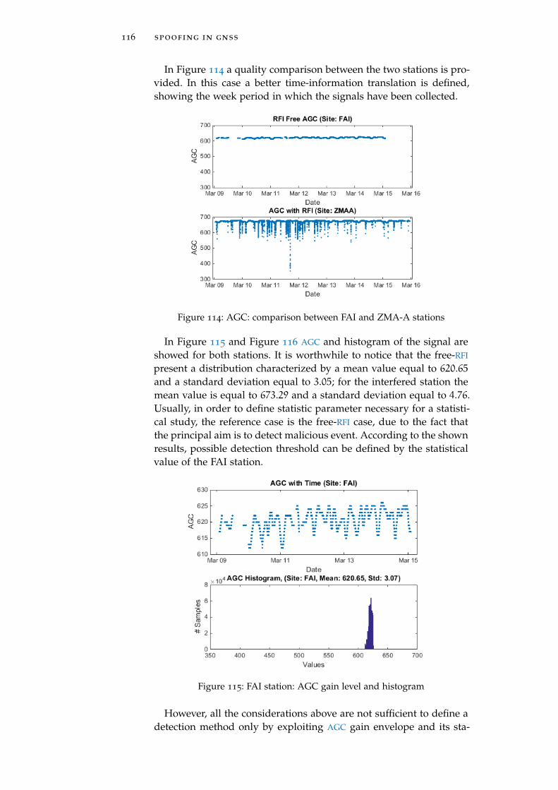
116 spoofing in gnss
In Figure 114 a quality comparison between the two stations is pro-vided. In this case a better time-information translation is defined,showing the week period in which the signals have been collected.
Figure 114: AGC: comparison between FAI and ZMA-A stations
In Figure 115 and Figure 116 AGC and histogram of the signal areshowed for both stations. It is worthwhile to notice that the free-RFI
present a distribution characterized by a mean value equal to 620.65and a standard deviation equal to 3.05; for the interfered station themean value is equal to 673.29 and a standard deviation equal to 4.76.Usually, in order to define statistic parameter necessary for a statisti-cal study, the reference case is the free-RFI case, due to the fact thatthe principal aim is to detect malicious event. According to the shownresults, possible detection threshold can be defined by the statisticalvalue of the FAI station.
Figure 115: FAI station: AGC gain level and histogram
However, all the considerations above are not sufficient to define adetection method only by exploiting AGC gain envelope and its sta-
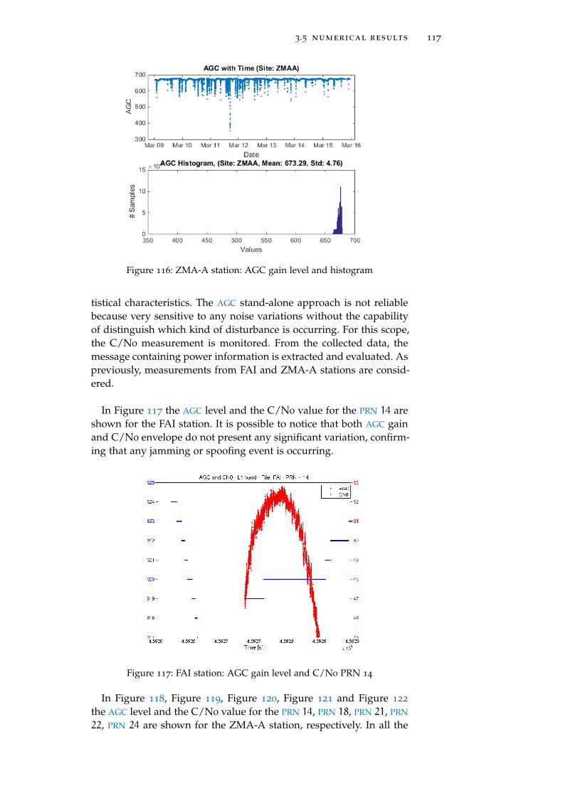
3.5 numerical results 117
Figure 116: ZMA-A station: AGC gain level and histogram
tistical characteristics. The AGC stand-alone approach is not reliablebecause very sensitive to any noise variations without the capabilityof distinguish which kind of disturbance is occurring. For this scope,the C/N0 measurement is monitored. From the collected data, themessage containing power information is extracted and evaluated. Aspreviously, measurements from FAI and ZMA-A stations are consid-ered.
In Figure 117 the AGC level and the C/N0 value for the PRN 14 areshown for the FAI station. It is possible to notice that both AGC gainand C/N0 envelope do not present any significant variation, confirm-ing that any jamming or spoofing event is occurring.
Figure 117: FAI station: AGC gain level and C/N0 PRN 14
In Figure 118, Figure 119, Figure 120, Figure 121 and Figure 122
the AGC level and the C/N0 value for the PRN 14, PRN 18, PRN 21, PRN
22, PRN 24 are shown for the ZMA-A station, respectively. In all the
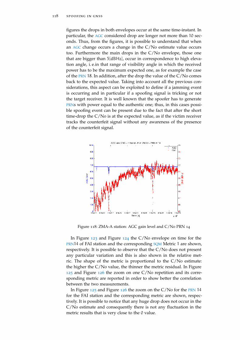
118 spoofing in gnss
figures the drops in both envelopes occur at the same time-instant. Inparticular, the AGC considered drop are longer not more than 10 sec-onds. Thus, from the figures, it is possible to understand that whenan AGC change occurs a change in the C/N0 estimate value occurstoo. Furthermore the main drops in the C/N0 envelope, those onethat are bigger than 5[dBHz], occur in correspondence to high eleva-tion angle, i. e.in that range of visibility angle in which the receivedpower has to be the maximum expected one, as for example the caseof the PRN 18. In addition, after the drop the value of the C/N0 comesback to the expected value. Taking into account all the previous con-siderations, this aspect can be exploited to define if a jamming eventis occurring and in particular if a spoofing signal is tricking or notthe target receiver. It is well known that the spoofer has to generatePRNs with power equal to the authentic one; thus, in this cases possi-ble spoofing event can be present due to the fact that after the shorttime-drop the C/N0 is at the expected value, as if the victim receivertracks the counterfeit signal without any awareness of the presenceof the counterfeit signal.
Figure 118: ZMA-A station: AGC gain level and C/N0 PRN 14
In Figure 123 and Figure 124 the C/N0 envelope on time for thePRN14 of FAI station and the corresponding SQM Metric 1 are shown,respectively. It is possible to observe that the C/N0 does not presentany particular variation and this is also shown in the relative met-ric. The shape of the metric is proportional to the C/N0 estimate:the higher the C/N0 value, the thinner the metric residual. In Figure125 and Figure 126 the zoom on one C/N0 repetition and its corre-sponding metric are reported in order to show better the correlationbetween the two measurements.
In Figure 125 and Figure 126 the zoom on the C/N0 for the PRN 14
for the FAI station and the corresponding metric are shown, respec-tively. It is possible to notice that any huge drop does not occur in theC/N0 estimate and consequently there is not any fluctuation in themetric results that is very close to the 0 value.
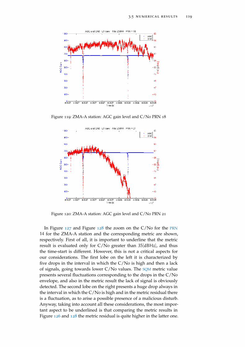
3.5 numerical results 119
Figure 119: ZMA-A station: AGC gain level and C/N0 PRN 18
Figure 120: ZMA-A station: AGC gain level and C/N0 PRN 21
In Figure 127 and Figure 128 the zoom on the C/N0 for the PRN
14 for the ZMA-A station and the corresponding metric are shown,respectively. First of all, it is important to underline that the metricresult is evaluated only for C/N0 greater than 35[dBHz], and thusthe time-start is different. However, this is not a critical aspects forour considerations. The first lobe on the left it is characterized byfive drops in the interval in which the C/N0 is high and then a lackof signals, going towards lower C/N0 values. The SQM metric valuepresents several fluctuations corresponding to the drops in the C/N0
envelope, and also in the metric result the lack of signal is obviouslydetected. The second lobe on the right presents a huge drop always inthe interval in which the C/N0 is high and in the metric residual thereis a fluctuation, as to arise a possible presence of a malicious disturb.Anyway, taking into account all these considerations, the most impor-tant aspect to be underlined is that comparing the metric results inFigure 126 and 128 the metric residual is quite higher in the latter one.
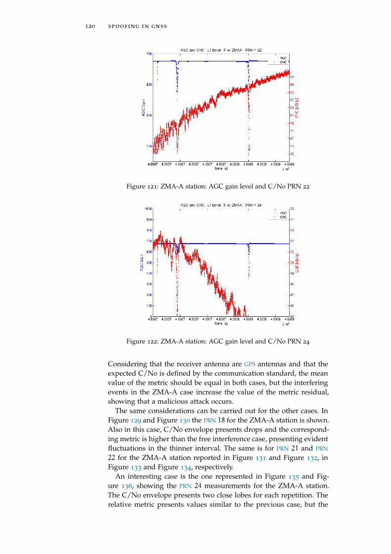
120 spoofing in gnss
Figure 121: ZMA-A station: AGC gain level and C/N0 PRN 22
Figure 122: ZMA-A station: AGC gain level and C/N0 PRN 24
Considering that the receiver antenna are GPS antennas and that theexpected C/N0 is defined by the communication standard, the meanvalue of the metric should be equal in both cases, but the interferingevents in the ZMA-A case increase the value of the metric residual,showing that a malicious attack occurs.
The same considerations can be carried out for the other cases. InFigure 129 and Figure 130 the PRN 18 for the ZMA-A station is shown.Also in this case, C/N0 envelope presents drops and the correspond-ing metric is higher than the free interference case, presenting evidentfluctuations in the thinner interval. The same is for PRN 21 and PRN
22 for the ZMA-A station reported in Figure 131 and Figure 132, inFigure 133 and Figure 134, respectively.
An interesting case is the one represented in Figure 135 and Fig-ure 136, showing the PRN 24 measurements for the ZMA-A station.The C/N0 envelope presents two close lobes for each repetition. Therelative metric presents values similar to the previous case, but the
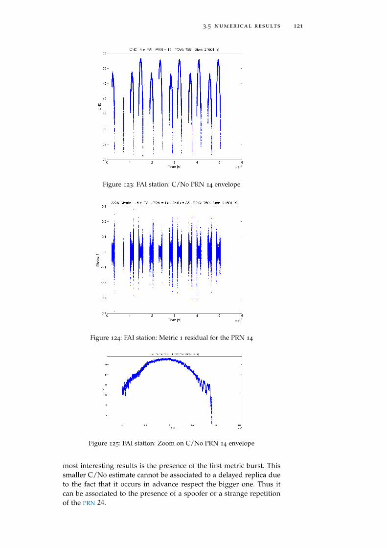
3.5 numerical results 121
Figure 123: FAI station: C/N0 PRN 14 envelope
Figure 124: FAI station: Metric 1 residual for the PRN 14
Figure 125: FAI station: Zoom on C/N0 PRN 14 envelope
most interesting results is the presence of the first metric burst. Thissmaller C/N0 estimate cannot be associated to a delayed replica dueto the fact that it occurs in advance respect the bigger one. Thus itcan be associated to the presence of a spoofer or a strange repetitionof the PRN 24.
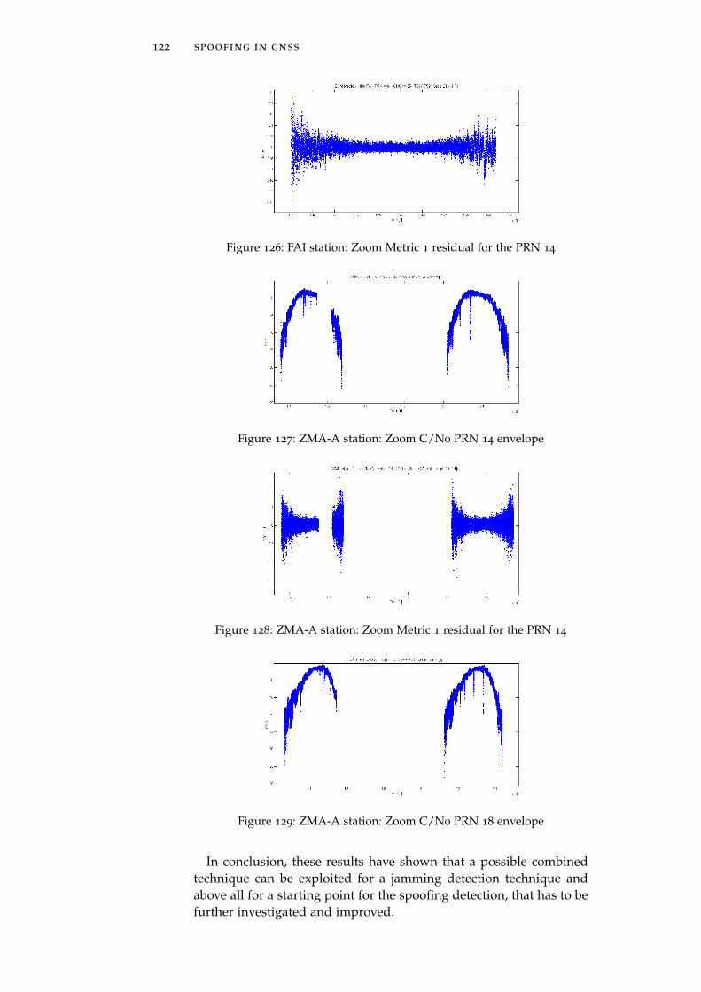
122 spoofing in gnss
Figure 126: FAI station: Zoom Metric 1 residual for the PRN 14
Figure 127: ZMA-A station: Zoom C/N0 PRN 14 envelope
Figure 128: ZMA-A station: Zoom Metric 1 residual for the PRN 14
Figure 129: ZMA-A station: Zoom C/N0 PRN 18 envelope
In conclusion, these results have shown that a possible combinedtechnique can be exploited for a jamming detection technique andabove all for a starting point for the spoofing detection, that has to befurther investigated and improved.
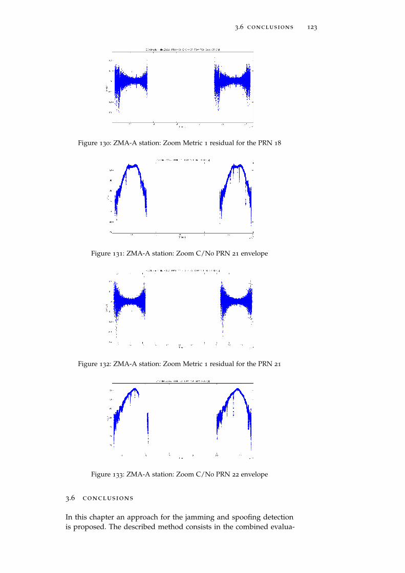
3.6 conclusions 123
Figure 130: ZMA-A station: Zoom Metric 1 residual for the PRN 18
Figure 131: ZMA-A station: Zoom C/N0 PRN 21 envelope
Figure 132: ZMA-A station: Zoom Metric 1 residual for the PRN 21
Figure 133: ZMA-A station: Zoom C/N0 PRN 22 envelope
3.6 conclusions
In this chapter an approach for the jamming and spoofing detectionis proposed. The described method consists in the combined evalua-
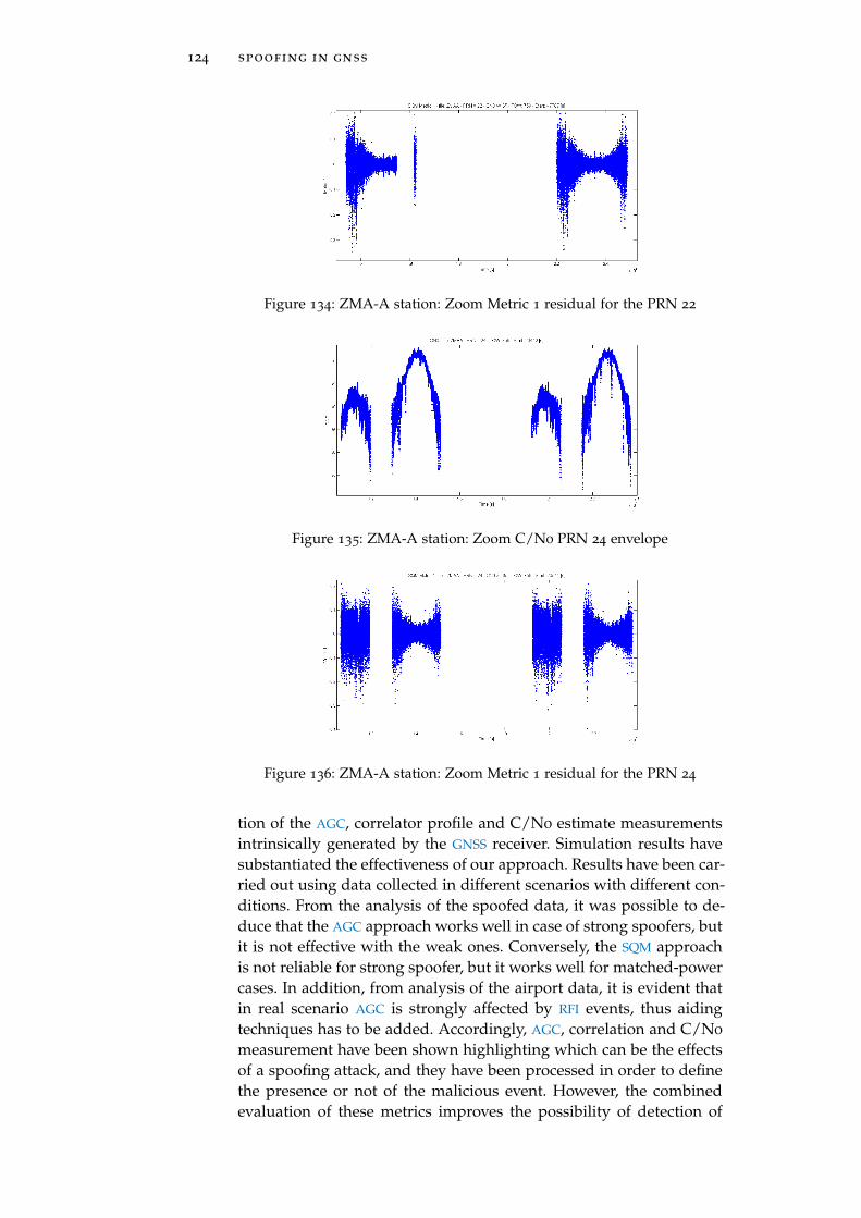
124 spoofing in gnss
Figure 134: ZMA-A station: Zoom Metric 1 residual for the PRN 22
Figure 135: ZMA-A station: Zoom C/N0 PRN 24 envelope
Figure 136: ZMA-A station: Zoom Metric 1 residual for the PRN 24
tion of the AGC, correlator profile and C/N0 estimate measurementsintrinsically generated by the GNSS receiver. Simulation results havesubstantiated the effectiveness of our approach. Results have been car-ried out using data collected in different scenarios with different con-ditions. From the analysis of the spoofed data, it was possible to de-duce that the AGC approach works well in case of strong spoofers, butit is not effective with the weak ones. Conversely, the SQM approachis not reliable for strong spoofer, but it works well for matched-powercases. In addition, from analysis of the airport data, it is evident thatin real scenario AGC is strongly affected by RFI events, thus aidingtechniques has to be added. Accordingly, AGC, correlation and C/N0
measurement have been shown highlighting which can be the effectsof a spoofing attack, and they have been processed in order to definethe presence or not of the malicious event. However, the combinedevaluation of these metrics improves the possibility of detection of
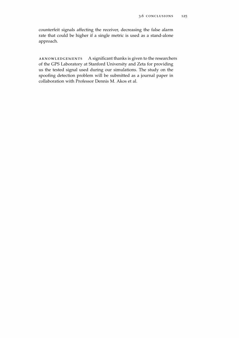
3.6 conclusions 125
counterfeit signals affecting the receiver, decreasing the false alarmrate that could be higher if a single metric is used as a stand-aloneapproach.
aknowledgements A significant thanks is given to the researchersof the GPS Laboratory at Stanford University and Zeta for providingus the tested signal used during our simulations. The study on thespoofing detection problem will be submitted as a journal paper incollaboration with Professor Dennis M. Akos et al.

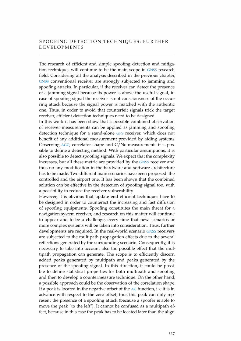
S P O O F I N G D E T E C T I O N T E C H N I Q U E S : F U RT H E RD E V E L O P M E N T S
The research of efficient and simple spoofing detection and mitiga-tion techniques will continue to be the main scope in GNSS researchfield. Considering all the analysis described in the previous chapter,GNSS conventional receiver are strongly subjected to jamming andspoofing attacks. In particular, if the receiver can detect the presenceof a jamming signal because its power is above the useful signal, incase of spoofing signal the receiver is not consciousness of the occur-ring attack because the signal power is matched with the authenticone. Thus, in order to avoid that counterfeit signals trick the targetreceiver, efficient detection techniques need to be designed.In this work it has been show that a possible combined observationof receiver measurements can be applied as jamming and spoofingdetection technique for a stand-alone GPS receiver, which does notbenefit of any additional measurement provided by aiding systems.Observing AGC, correlator shape and C/N0 measurements it is pos-sible to define a detecting method. With particular assumptions, it isalso possible to detect spoofing signals. We expect that the complexityincreases, but all these metric are provided by the GNSS receiver andthus no any modification in the hardware and software architecturehas to be made. Two different main scenarios have been proposed: thecontrolled and the airport one. It has been shown that the combinedsolution can be effective in the detection of spoofing signal too, witha possibility to reduce the receiver vulnerability.However, it is obvious that update end efficient techniques have tobe designed in order to counteract the increasing and fast diffusionof spoofing equipments. Spoofing constitutes the main threat for anavigation system receiver, and research on this matter will continueto appear and to be a challenge, every time that new scenarios ormore complex systems will be taken into consideration. Thus, furtherdevelopments are required. In the real-world scenario GNSS receiversare subjected to the multipath propagation effects due to the severalreflections generated by the surrounding scenario. Consequently, it isnecessary to take into account also the possible effect that the mul-tipath propagation can generate. The scope is to efficiently discernadded peaks generated by multipath and peaks generated by thepresence of the spoofing signal. In this direction, it could be possi-ble to define statistical properties for both multipath and spoofingand then to develop a countermeasure technique. On the other hand,a possible approach could be the observation of the correlation shape.If a peak is located in the negative offset of the AC function, i. e.it is inadvance with respect to the zero-offset, thus this peak can only rep-resent the presence of a spoofing attack (because a spoofer is able tomove the peak "to the left"). It cannot be confused as a multipath ef-fect, because in this case the peak has to be located later than the align
127
128 spoofing in gnss
time-instant due to the nature of the multipath propagation. Other so-lutions are represented by the improvement of the techniques basedon the observation of the C/N0 estimation in function of the elevationangle and in comparison with contemporary drops in the AGC gainlevel (as defined in Chapter 3). In addition, possible solution is repre-sented by the implementation of spare searching correlators that can"look for" energy outside the main peak and thus signals that have awider bandwidth with respect to the receiver. This technique can beefficient but with a higher complexity because more correlators arerequired. Conversely, the SQM techniques are more probable due tothe fact that measurements are provided by the GNSS receiver.
In conclusion, new challenges are defined by different communi-cation complex systems. Due to the increasing diffusion of civil in-frastructure relying on GNSS, these new challenges will need to besolved trying to not modify the system architecture and preservingthe technical knowledge of the current positioning systems.
C O N C L U D I N G R E M A R K S
In this dissertation, techniques for possible enhancement of the per-formance in satellite navigation systems have been studied and de-signed. The common topic between the two presented part is the in-terfering threat in GNSS.
In the first part the attention has been focused on the study of pos-sible detection and mitigation techniques for structured interferingsignals. In particular, a jamming detection method performed in thefrequency domain has been provided. The mathematical tool of WT
has been exploited in order to detect discontinuities in interfering PSD
envelope. The same techniques has been applied in time-domain inorder to define the duty-cycle of an interfering waveform. Thus, it ispossible to define the activity in time of the jamming source. Succes-sively, an improvement of an existing technique has been described.An analytical study of the chirp signal has been evaluated and ana-lytical AC function has been expressed in a closed form. Additionalresults in terms of cancellation performance have been showed inorder to improve proposed algorithm (in [P4]). Moving from theseresults, the aforementioned algorithm has been applied in a differ-ent and harsh scenario. In this case, the interfering signal has beenconsidered affected by multipath propagation (UMTS channel), thenresulting from the contribution of the delayed replicas. The describedalgorithm has been tested also for this particular case. Numerical re-sults have shown that the provided method still works properly de-tecting and canceling multipath jamming signal, also in presence ofthe useful GNSS signal. Thus, its effectiveness has been demonstratedby means of computer simulations and emulations, showing its capa-bilities.
In the second part of this dissertation, the attention has been fo-cused on the most sophisticated interfering waveform, the spoofingsignal. Since spoofing signal has become a very important topic, sev-eral literature works have been presented in order to provide validsolutions of different kinds. After a deep review of existing works,a possible solution in spoofing detection has been presented. Ourapproach has been based on the jointly observation of different mea-surement outputs from three main blocks inside the GNSS receiver.The study has been centered on the analysis of the output signal ofthe AGC, the correlator and the estimation of the C/N0. Exploitingthese envelopes in a jointly way, a possible detection approach hasbeen defined, by the evaluation of data collected in controlled sce-nario and airport area.
129

B I B L I O G R A P H Y
[1] A novel multipath interference cancellation scheme for rakechannel estimation. In Vehicular Technology Conference, 2001. VTC2001 Spring. IEEE VTS 53rd, 2001.
[2] Evaluation of multipath effects on interference cancellation ingnss using space-time based array processing. In Electromag-netic Noise and Interference Control Session, Ursi General Assembly,08/2008 2008.
[3] A multipath mitigation algorithm in global navigation satellitesystems arrays using independent component analysis. In Wire-less Communications, Networking and Information Security (WCNIS),2010 IEEE International Conference on, 06/2010 2010.
[4] D.M. Akos. Who’s afraid of the spoofer? gps/gnss spoofing de-tection via automatic gain control (agc). In Journal of the Instituteof Navigation, Navigation, volume 59, 2012.
[5] K. Ali, Xin Chen, and F. Dovis. On the use of multipath es-timating architecture for spoofer detection. In Localization andGNSS (ICL-GNSS), 2012 International Conference on, pages 1–6,June 2012.
[6] K. Ali, E.G. Manfredini, and F. Dovis. Vestigial signal defensethrough signal quality monitoring techniques based on joint useof two metrics. In Position, Location and Navigation Symposium -PLANS 2014, 2014 IEEE/ION, pages 1240–1247, May 2014.
[7] Asghar Tabatabaei Balaei and Dennis Akos Andrew G. Demp-ster. Quantization degradation of gnss signal quality in the pres-ence of cw rfi. In IEEE International Symposium on Spread SpectrumTechniques and Applications (ISSSTA’08), In Proceedings, pages 42–47, 2008.
[8] Asghar Tabatabaei Balaei, Jinghui Wu, and Andrew G. Demp-ster. Comparison between gps and galileo satellite availabilityin the presence of cw interference. In International Symposium onGPS/GNSS (IGNSS), In Proceedings, 2007.
[9] A.T. Balaei, B. Motella, and Dempster A.G. Gps interference de-tected in sydney-austalia. In International Global Navigation Satel-lite Systems Society IGNSS Symposium 2007, Proceedings of, 2007.
[10] A.T. Balalei, J. Barnes, and A.G. Dempster. Characterization ofinterference effects on gps signal carrier phase error. In SSC(2005), 2005.
[11] F. Bastide, D. Akos, C. Macabieu, and B. Roturier. Automaticgain control (agc) as an interference assessment tool. In ION
131
132 bibliography
GNSS 16th. International Technical Meeting of the Satellite Divisionof the Institute of Navigation (ION GPS/GNSS 2003), Proceedings of,pages 2042–2053, September 2003.
[12] R. Bauernfeind, I. Kramer, H. Beckmann, B. Eissfeller, andV. Vierroth. In-car jammer interference detection in automotivegnss receivers and localization by means of vehicular communi-cation. In Integrated and Sustainable Transportation System (FISTS),2011 IEEE Forum on, pages 376–381, 2011.
[13] J.W. Betz. Effect of narrowband interference on gps code trackingaccuracy. In National Technical Meeting of the Institute of NavigationION-NTM 2000, Proceedings of, pages 16–27, 2000.
[14] J.W. Betz. Effect of partial-band interference on receiver estima-tion of c/n0: Theory. In National Technical Meeting of the Instituteof Navigation ION-NTM 2001, Proceedings of, pages 16–27, 2001.
[15] D. Borio, S. Savasta, and L. LoPresti. On the dvb-t coexistencewith galileo and gps systems. In 3rd ESA Workshop on SatelliteNavigation User Equipment Technologies (NAVITEC 2006), Proceed-ings of, 2006.
[16] R Boucher and Joseph C. Hassab. Analysis of discrete implemen-tation of generalized cross correlator. Acoustic, Speech and SignalProcessing, IEEE Transaction on, 29(3):609–611, Jun 1981.
[17] A. Broumandan, A. Jafarnia-Jahromi, V. Dehghanian, J. Nielsen,and G. Lachapelle. Gnss spoofing detection in handheld re-ceivers based on signal spatial correlation. In Position Locationand Navigation Symposium (PLANS), 2012 IEEE/ION, April 2012.
[18] A. Brown, D Reynolds, D. Roberts, and S. Serie. Interference lo-calisation trials using adaptive antennas array. In The Institute ofNavigation of ION GPS 1999, Proceedings of, pages 137–142, 1999.
[19] A. Cavaleri, B. Motella, M. Pini, and M. Fantino. Detection ofspoofed gps signals at code and carrier tracking level. In Satel-lite Navigation Technologies and European Workshop on GNSS Sig-nals and Signal Processing (NAVITEC), 2010 5th ESA Workshop on,pages 1–6, Dec 2010.
[20] Saeed Daneshmand, Ali Jafarnia-Jahromi, Ali Broumandon, andGérard Lachapelle. Gps spoofing detection using raim with inscoupling. In the 25th International Technical Meeting of The SatelliteDivision of the Institute of Navigation (ION GNSS 2012),Proceedingsof, pages 1233–1243, September 2012.
[21] I. Daubechies. The wavelet transform, time-frequency localiza-tion and signal analysis. Information Theory, IEEE Transactions on,36(5):961–1005, 1990.
[22] P.G.M. de Jong, T. Arts, A.P.G. Hoeks, and R.S. Reneman. Deter-mination of tissue motion velocity by correlation interpolation
bibliography 133
of pulsed ultrasonic echo signals. Ultrasonic Imaging, 12(2):84–98,Apr. 1990.
[23] P.G.M. de Jong, T. Arts, A.P.G. Hoeks, and R.S. Reneman. Ex-perimental evaluation of the correlation interpolation techniqueto measure regional tissue velocity. Ultrasonic Imaging, 13(2):145–161, Apr. 1991.
[24] GPS Directorate. Systems engineering and integration Interface Spec-ification IS-GPS-200G.
[25] F. Dovis and L. Musumeci. Use of wavelet transforms for inter-ference mitigation. In Localization and GNSS (ICL-GNSS), 2011International Conference on, pages 116–121, June 2012.
[26] ETSI. Universal mobile telecommunications system. Technicalreport, ETSI TR 101 112 v3.2.0, 1998.
[27] M. Fantino, A. Molino, P. Mulassano, M. Nicola, and M. Rao.Signal quality monitoring: Correlation mask based on ratio testmetrics for multipath detection. In IGNSS 2009, Gold Coast, Aus-tralia, 12/2009 2009.
[28] G. Gabelli. Code Synchronization and Interference Management Tech-niques for Satellite Navigation and Communications. PhD thesis,University of Bologna, 2014.
[29] G. Gabelli, R. Casile, A. Guidotti, and G.E. Corazza. Gnss jam-ming interference: Characterization and cancellation. In 2013International Technical Meeting of The Institute of Navigation, Pro-ceedings of, pages 828–834, 2013.
[30] J.C. Grabowski. Field observations of personal privacy devices.In International Technical Meeting of The Institute of Navigation, Pro-cedings of, Newport Beach, CA, January 2012, pages 689–741, 2012.
[31] Joseph C. Grabowski. Personal privacy jammers. In GPS World,2012.
[32] K. Gromov, D. Akos, D. Pullen, and P. Enge. Gidl: Generalizedinterference detection and localization system. In 13th Interna-tional Technical Meeting of the Satellite Division of The Institute ofNavigation (ION GPS 2000), Proceedings of, pages 447–457, 2000.
[33] D Hambling. Gps chaos: How a 30$ box can jam your life. Tech-nical report, New Scientist, 2011.
[34] Guenter Hein, Felix Kneissl, Jose-Angel Avila-Rodriguez, andStefan Wallner. Authenticating gnss: Proofs against spoofs, part1. July/August 2007.
[35] Guenter Hein, Felix Kneissl, Jose-Angel Avila-Rodriguez, andStefan Wallner. Authenticating gnss: Proofs against spoofs, part2. INSIDE GNSS, September/October 2007:71–78, 2007.
134 bibliography
[36] Todd E. Humphreys, Brent M. Ledvina, Mark L. Psiaki, Brady W.O’Hanlon, and Paul M Jr Kintner. Assessing the spoofing threat:development of a portable gps civilian spoofer. In ION GNSS21st. International Technical Meeting of the Satellite Division, Pro-ceedings of, 2008.
[37] Global Positioning System Wing Systems Engineering & Inte-gration. Navstar gps space segment/navigation user interfacesinterface specification - is-gps-200 revision e. Technical report,GPSW, June, 8 2010.
[38] Usman Muhammad Iqbal and Samsung Lim. Legal and ethi-cal implications of gps vulnerabilities. In Journal of InternationalCommercial Law & Technology, volume 3, July 2008.
[39] O. Isoz and D. Akos. Development of a deployable low costinterference detection and localization system for the gnss l1/e1
band. In Satellite Navigation Technologies and European Workshopon GNSS Signals and Signal Processing (NAVITEC), 2010 5th ESAWorkshop on, pages 1–4, 2010.
[40] O. Isoz, A.T. Balalei, and D. Akos. Interference detection andlocalization in gps l1 band. In Proceedings of ION NTM 2010, SanDiego, CA, 2010.
[41] O. Isoz, D. Akos, T. Lindgren, C.C. Sun, and S.S. Jan. Assess-ment of gps l1/galileo e1 interference monitoring system forthe airport environment. In ION GNSS 24th. International Tech-nical Meeting of the Satellite Division of the Institute of Navigation(ION GPS/GNSS 2011), Proceedings of, pages 1920–1930, Septem-ber 2011.
[42] Ali Jafarnia-Jahromi, Ali Broumandan, John Nielsen, and GérardLachapelle. Pre-despreading authenticity verification for gps l1ca signals. Navigation, 61(1).
[43] Ali Jafarnia Jahromi. GNSS Signal Authenticity Verification in thePresence of Structural Interference. PhD thesis, University of Cal-gary, 2013.
[44] A. Jovanovic, C. Botteron, and P.-A. Farine. Multi-test detectionand protection algorithm against spoofing attacks on gnss re-ceivers. In Position, Location and Navigation Symposium - PLANS2014, 2014 IEEE/ION, pages 1258–1271, May 2014.
[45] E.D. Kaplan and C.J. Hegarty. Understanding GPS: Principlesand Applications. Artech House mobile communications series.Artech House, 2005.
[46] A.J. Kerns, D.P. Shepard, J.A. Bhatti, and T.E. Humphreys. Un-manned aircraft capture and control via gps spoofing. In NationalWorkshop on the New Clockwork for Time-Critical Cyber-Physical Sys-tems, volume 31, 2014.
bibliography 135
[47] S. Khanafseh, N. Roshan, S. Langel, Fang-Cheng Chan, M. Jo-erger, and B. Pervan. Gps spoofing detection using raim with inscoupling. In Position, Location and Navigation Symposium - PLANS2014, 2014 IEEE/ION, pages 1232–1239, May 2014.
[48] T. Kraus, R. Bauernfeind, and B. Eissfeller. Survey of in-carjammers-analysis and modeling of the rf signals and if samples(suitable for active signal cancellation). In 24th International Tech-nical Meeting of The Satellite Division of the Institute of Navigation(ION GNSS 2011), Proceedings of, pages 430–435, 2011.
[49] Brent M. Ledvina, William J. Bencze, Bryan Galusha, and IssacMiller. An in-line anti-spoofing device for legacy civil gps re-ceivers. In the 2010 International Technical Meeting of The Instituteof Navigation, Proceedings of, pages 698–712, January 2010.
[50] S. Lo, David De Lorenzo, Per Enge, D. Akos, and P. Bradley.Signal authentication: A secure civil gnss for today. Inside GNSS,2009.
[51] M. Luo, G. Xie, D. Akos, and S. Pullen. Radio frequency inter-ference validation testing for laas using the standford integritymonitor testbed. In Proceedings of ION NTM 2003, Anaheim, CA,2003.
[52] R.G. Lyons. Understanding digital signal processing. 3rd edn. Pren-tice Hall Signal PIR. Upper Saddle River, 2010.
[53] L. Musumeci and F. Dovis. A comparison of transformed-domain techniques for pulsed interference removal on gnss sig-nals. In Localization and GNSS (ICL-GNSS), 2012 International Con-ference on, pages 1–6, June 2012.
[54] L. Musumeci and F. Dovis. Performance assessment of waveletbased techniques in mitigatin narrow-band interference. In Lo-calization and GNSS (ICL-GNSS), 2013 International Conference on,pages 1–6, June 2013.
[55] A. Ndili and P. Enge. Gps receiver autonomous interference de-tection. In Position Location and Navigation Symposium, IEEE 1998,pages 123–130, Apr 1998.
[56] John Nielsen, Ali Broumandan, and Gérard Lachapelle. Gnssspoofing detection for single antenna handheld receivers. Navi-gation, 58(4).
[57] Brady W. O’Hanlon, Mark L. Psiaki, Jahshan A. Bhatti, Daniel P.Shepard, and Todd E. Humphreys. Real-time gps spoofing detec-tion via correlation of encrypted signals. In Journal of The Instituteof Navigation,NAVIGATION, pages 267–278, September 2013.
[58] I. G. Petrovski. GPS, GLONASS, Galileo, BeiDou for Mobile De-vices. United Kingdom: Cambrige University Press. CambrigeUniversity Press, 2014.
136 bibliography
[59] R.E. Phelts. Multicorrelator techniques for robust mitigation of threatsto GPS signal quality. PhD thesis, Stanford University, October2001.
[60] Mark L. Psiaki, Brady W. O’Hanlon, Jahshan A. Bhatti, Daniel P.Shepard, and Todd E. Humphreys. Civilian gps spoofing de-tection based on dual-receiver correlation of military signals. In24th International Technical Meeting of The Satellite Division of the In-stitute of Navigation (ION GNSS 2011),Proceedings of, pages 2619–2645, September 2011.
[61] RAE. The royal academy of engineering, global navigation spacesystems: Reliance and vulnerabilities. Technical report, 2011.
[62] K. Deergha Rao, M.N.S. Swamy, and E.I. Plotkin. Anti-spoofingfilter for accurate gps navigation. In the 13th International Tech-nical Meeting of the Satellite Division of The Institute of Navigation(ION GPS 2000),Proceedings of, pages 1536–1541, September 2000.
[63] F. Reed, P. Feintuch, and N. Bershad. Time delay estimationusing the lms adaptive filter - static behaviour. IEEE Trans AcoustSpeech Signal Process.
[64] M. Sahmoudi and M.G. Amin. Fast iterative maximum-likelihood algorithm (fimla) for multipath mitigation in the nextgeneration of gnss receivers. Wireless Communications, IEEE Trans-actions on, 7(11):4362–4374, 2008.
[65] J. Sanz Subirana, J.M. Juan Zornoza, and Hernandéz-Pajares.GNSS Data Processing (Vol. I.: Fundamentals and Algorithms). Esa.Esa, 2013.
[66] L. Scott. Anti-spoofing & authenticated signal architectures forcivil navigation systems. In 16th International Technical Meeting ofthe Satellite Division of The Institute of Navigation (ION GPS/GNSS2003),Proceedings of, pages 1543–1552, September 2003.
[67] D. Shepard and Todd E. Humphreys. Characterization of re-ceiver response to a spoofing attack. In the ION GNSS Meeting,Proceedings of, 2011.
[68] Daniel P. Shepard, Jahshan A. Bhatti, Todd E. Humphreys, andAaron A. Fansler. Evaluation of smart grid and civilian uav vul-nerability to gps spoofing attacks. In the ION GNSS Meeting,Proceedings of, 2012.
[69] Daniel P. Shepard, Todd E. Humphreys, and Aaron A. Fansler.Evaluation of the vulnerability of phasor measurement units to{GPS} spoofing attacks. International Journal of Critical Infrastruc-ture Protection, 5(3-4):146–153, 2012.
[70] K. Sheridan, Y. Ying, and T. Whitworth. Pre- and post- correla-tion interference detection within software defined radio. In 25th

bibliography 137
International Technical Meeting of The Satellite Division of the Insti-tute of Navigation (ION GNSS 2012), Proceedings of, pages 3542–3548, 2012.
[71] M. Trinkle and D.A. Gray. Interference localisation trials usingadaptive antennas array. In The Institute of Navigation of ION GPS2002, Proceedings of, pages 613–619, 2002.
[72] European Union. European GNSS (Galileo) open service signal inspace interface control document.
[73] A.J. Van Dierendonck. GPS Receivers. Global Positioning System:Theory and Application. Parkinson, B. and Spilker, J.J, JR., Ed .,1996.
[74] John A. Volpe. Vulnerability assessment of the transportation in-frastructure relying on the global positioning system. Technicalreport, National Transportation Systems Center, 2001.
[75] Phillip Ward. Monograph on gps antispoofing. In 8th Inter-national Technical Meeting of the Satellite Division of The Instituteof Navigation (ION GPS 1995),Proceedings of, pages 1563–1571,September 1999.
[76] Jon S. Warner and Roger G. Johnston. A simple demonstrationthat the Global Positioning System (GPS) is vulnerable to spoofing.Journal of Security Administration.
[77] Hengqing Wen, Peter Yih-Ru Huang, John Dyer, Andy Archinal,and John Fagan. Countermeasures for gps signal spoofing. Inthe 18th International Technical Meeting of the Satellite Division ofThe Institute of Navigation (ION GNSS 2005),Proceedings of, pages1285–1290, September 2005.
[78] K. Wesson, D. Shepard, and T.E. Humphreys. Straight talk onanti-spoofing: Securing the future of pnt. In GPS World, 2012.
[79] K.D. Wesson, T.E. Humphreys, and B.L. Evans. Position paper:Secure time transfer for cps. In National Workshop on the NewClockwork for Time-Critical Cyber-Physical Systems, 2012.
[80] K.D. Wesson, B.L. Evans, and T.E. Humphreys. A combined sym-metric difference and power monitoring gnss anti-spoofing tech-nique. In Global Conference on Signal and Information Processing(GlobalSIP), 2013 IEEE, pages 217–220, December 2013.
[81] Shepard Daniel P. Bhatti Jahshan A. Humphreys Todd E. Wes-son, Kyle D. An evaluation of the vestigial signal defense forcivil gps anti-spoofing. In the 24th International Technical Meetingof The Satellite Division of the Institute of Navigation (ION GNSS2011),Proceedings of, pages 2646–2656, September 2011.
[82] Nathan A. White, Peter S. Maybeck, and Stewart L. DeVilbiss.Mmae detection of interference/jamming and spoofing in adgps-aided inertial system. In the 11th International Technical
138 bibliography
Meeting of the Satellite Division of The Institute of Navigation (IONGPS 1998),Proceedings of, September 1998.
[83] M. Wildemeersch, E. Cano Pons, A. Rabbachin, and J. FortunyGuasch. Impact study of unintentional interference on gnss re-ceivers. Technical Report EUR 24742 EN, EC Joint Research Cen-tre, 2010.
[84] J. Yi, Z. Shu-fang, S. Xiao-wen, Z. Jing-bo, and H. Qing. A newrake-based multipath estimation algorithm in gnss receivers. InImage and Signal Processing (CISP), 2010 3rd International Congresson, volume 9, pages 4313–4317, 10/2010 2010.
[85] Lei Zhang and Xiaolin Wu. On the application of cross correla-tion function to subsample discrete time delay estimation. DigitalSignal Processing, 16(6):682–694, Nov. 2006.
A C K N O W L E D G M E N T S
Con questa tesi porto a termine il mio Dottorato, percorso durato treanni durante i quali ho potuto mettere alla prova ed arricchire la miapersonalità. Quest’esperienza mi ha concesso di lavorare, vivere e con-dividere gran parte del mio tempo con tante persone, ciascuna dellequali mi ha lasciato qualcosa. Per questo vorrei ringraziare tutte loroper avermi concesso il loro tempo, i loro sorrisi e il loro appoggio neimomenti un po’ più bui. I loro consigli e le loro attenzioni ed il loromodo di comunicare con me hanno contribuito in buona parte a ciòche sono oggi. La prima persona che ringrazio è Giovanni, che è statouna guida durante questo mio percorso, e che mi ha trasmesso profes-sionalità e dedizione. La sua accoglienza nel gruppo di ricerca mi hatrasmesso fiducia, coraggio e interesse, e donato l’opportunità di af-frontare un percorso tortuoso ma soddisfacente. Ringrazio tutti i mieicolleghi del gruppo Digicomm che ho conosciuto nel corso dei treanni. Ho condiviso con loro momenti faticosi e difficili ma anche tantesoddisfazioni. Ognuno di loro mi ha donato qualcosa e sebbene ab-biano intrapreso strade diverse è comunque per me importante dedi-care loro un pensiero per ringraziarli dell’affetto mostratomi. Quindiun caloroso grazie va a Giulio, Daniele, Alberto, Francesco, Lina, Ste-fano, Vahid, Alessandro e Sergio, ed anche alle nuovissime leve cheho conosciuto alla fine del mio percorso. Un grazie è rivolto anche adAlessandro Vanelli Coralli che pur non essendo il mio supervisore hacontribuito alla mia crescita umana e professionale.
A special thanks is given to Prof. Dennis Akos and to his researchgroup, who hosted me at the University of Colorado, Boulder. It hasbeen really an honor to work with them, and it has been a wonderfulopportunity of growth.
Vorrei ringraziare tutti coloro che mi hanno sempre affiancato intutto ciò che ho fatto e che faccio ogni giorno dandomi la forza dicontinuare a crescere e migliorare. Quelle persone con cui ho condi-viso tanto e che mi hanno reso la persona che sono oggi. Ringraziotutti gli amici quelli di vecchia data e quelli più recenti, per avermisostenuto nei momenti difficili ed esaltato in quelli più felici. Ungrazie incommensurabile va a Stefano, una persona veramente spe-ciale per me. Lo ringrazio per l’esserci sempre stato, disponibile, pre-muroso e paziente ma al tempo giusto anche severo. Lo ringrazio perla sua voglia di farmi sentire all’altezza e di vedermi realizzata e perl’infinita dolcezza e pazienza avuta anche nei momenti meno felici.Infine, devo ringraziare la mia famiglia. Mio padre, mia madre edi miei due fratelli sono sempre stati i miei primi sostenitori. Hannosempre creduto in me. Senza nessuna esitazione hanno accolto ognimia decisione con felicità ed entusiasmo. Li ringrazio per tutto ciò chemi hanno trasmesso ed insegnato, e per l’immenso affetto donatomiogni giorno.
Semplicemente, grazie a tutti . . .
139