Embed Size (px)
Citation preview

.“
.*
CIC-14 REPORT COLLECTION
LA-5378 REPRODUCTION—COPY UC-34
*.3
Reporting Date: Aug.Issued: June 1974
1973
Initial Value Problems of the
Rayleigh-Taylor Instability Type
by
Roy A. Axford*
●Consultant. Permanent address: 206 Nuclear EngineeringLaboratory, University of Illinois at Urbana - Champaign,Urbana, Illinois 61801.
_—_— ---—————— -—————-—
L?’10s alamos,
scientific laboratory\ of the university of California
.LOS ALAMOS, NEW
ii
ICIC-14 REPORT COLLECTION
~EPRODUCTION.-
COPY
MEXICO 87544
-—
uNITED STATES
ATOMIC ENERGY COMMISSION
CONTRACT W-7405 -ENG. 36

This report was prepared as an account of work sponsored by the United
States Government. Neither the United States nor the United States AtomicEnergy Commission, nor any of their employees, nor any of their contrac-
tors, subcontr=tors, or their employees, makes any warranty, express or im-plied, or assumes any legal liability or responsibility for the accuracy, com-pleteness or usefulness of any information, apparatus, product or process dis-closed, or represents that its use would not infringe privately owned rights.
Printed in the United States of America. Available fromNational Technical Information Service
U.S. Department of Commerce5285 Port Royal Road
Springfield, Virginia 22151Price: Printed Copy $4.00 Microfiche $1.45
-1
.

CONTENTS
“
.
.
ABSTRACT. . . . . . . . . . . . . . . . . . . . . . . . . . . . . . . . . . . . . . . . . .
1. INTRODUCTION . . . . . . . . . . . . . . . . . . . . . . . . . . . . . . . . . . . . .
2. ALTERNATIVE FUNDAMENTAL FORMULATIONS . . . . . . . . . . . . . . . . . . . . . . . . .
2.1 Stream Function Formulation . . . . . . . . . . . . . . . . . . . . . . . . . . .
2.2 Velocity Potential Formulation . . . . . . . . . . . . . . . . . . . . . . . . . .
2.3 DNSFormulation. . . . . . . . . . . . . . . . . . . . . . . . . . . . . . . . .
3. SOLUTIONS OF TAYLOR INSTABILITY INITIAL VALUE PROBLEMS FOR INVISCID FLUIDS . . . . . .
3.1 Solutions for Two-Fluid, Double Half-Space, Single-InterfaceConfigurationwith Constant Acceleration . . . . . . . . . . . . . . . . . . . . .
3.1.1 General Result with Surface Tension and an ArbitraryInitial Interface Perturbation . . . . . . . . . . . . . . . . . . . . . .
3.1.2 An Initial Cosine PerturbationResult . . . . . . . . . . . . . . . . . . .
3.1.3 An Initial Hump PerturbationResult . . . . . . . . . . . . . . . . . . . .
3.1.4 An Initial Groove PerturbationResult . . . . . . . . . . . . . . . . . . .
3.2 Solutions for a Fluid Sheet with Constant Acceleration . . . . . . . . . . . . . .
3.2.1 General Result with Surface Tension and Arbitrary InitialPerturbationsontheTwo Surfaces . . . . . . . . . . . . . . . . . . . . .
3.2.2 Result for Initial Cosine Perturbationson the Two Surfaceswith the Same Wave Numbers and with a Specified Phase Difference . . . . .
3.3 Solutions for Time-DependentAccelerations . . . . . . . . . . . . . . . . . . . .
3.3.1
3.3.2
3.3.3
3.3.4
Forms of Time-DependentAccelerationsConsidered . . . . . . . . . . . . .
DNS FormulationApplications to the Double Half-Space Problemwith Time-DependentAccelerations . . . . . . . . . . . . . . . . . . . . .
Motions of the Surfaces of a Fluid Sheet Induced by Time-DependentAccelerations. . . . . . . . . . . . . . . . . . . . . . . . . .
Responses of the Interfacesof a Three-Region CompositeDomain to Time-DependentAccelerations . . . . . . . . . . . . . . . . . .
4. SOLUTIONS OF TAYLOR INSTABILITY INITIAL VALUE PROBLEMS FOR VISCOUS FLUIDS . . . . . . .
4.1
4.2
4.3
-—
Solutions for a Half-Space Configurationwith Constant A~celeration . . . . . . .
4.1.1 Application of the Stream Function Formulation . . . . . . . . . . . . . .
4.1.2 Application of the DNS Formulation . . . . . . . . . . . . . . . . . . . .
4.1.3 Inversion of the Laplace Transform . . . . . . . . . . . . . . . . . . . .
Solution for a Viscous Fluid Sheet with Constant Acceleration . . . . . . . . . .
InterfaceMotion between Two Half-Spaces of Incompressible,ViscousFluids under Constant Acceleration . . . . . . . . . . . . . . . . . . . . . . .
——— ,-—.
—. ,.
.
y-- r-. ., . . .
1
1
2
2
4
6
7
7
9
9
9
10
10
14
15
1s
15
21
25
29
29
29
31
33
34
39..=-
-_.._. .. ..
-*.
.+--
iii
INITIAL VALUE PROBLEMS OF THE RAYLEIGH-TAYLORINSTABILITYTYPE
“
by
Roy A. Axford
ABSTRACT
Rayleigh-Taylorinstability initial value problems are set up interms of the velocity potential formulation for inviscid fluids, thestream function formulation for viscous fluids, and the DNS formula-tion, which is applicable to both inviscid and viscous fluids. Explic-it solutions of these initial value problems are obtained for half-spaces, double half-spaces, thick and thin sheets, and stratifiedmediafor both time-independentand time-dependentimposed accelerations.
1. INTRODUCTION
This report is the first of a contemplated
series that will deal with Rayleigh-Taylorinsta-
bility phenomena. Our objective is to provide a
systematic, expositorydevelopment of Rayleigh-
Taylor instability,together with new analytic and
quantitativeresults.
Emphasis is given to alternative formulations
and methods of solution applicable to Rayleigh-
Taylor instabilityinitial value problems. We con-
sider the existence of stability or instabilityand
follow the actual time response of interfacesre-
gardless of stability or instabilityoccurrence.
Work pertaining to Rayleigh-Taylorinstabil-
ity phenomena for the 90-yr period from 1883 to
1973 is contained in Refs. 1-45. Additional ref-
erences are cited in Refs. 1-45 and in NASA Liter-
ature Search No. 12616 for the period from 1964 to
.July 28, 1970.
A direct considerationof the equations of
continuity and motion and the introductionof a
velocity potential might be described as the stand-
ard starting points for the determinationof the
motions of free surfaces or interfacesbetween dis-
similar media when accelerationsperpendicularto
the mean positions of these surfaces are imposed.
However, the velocity potential formulation is of
little value in Rayleigh-Taylorinstability initial
value problems for viscous fluids.
The last paragraph of Sec. 2 in a paper by
Bellman and Pennington7 states: *’Notethat in this
present Section one cannot satisfy the condition
that the velocities be zero when t = O. Apparently
because of the linearizationperformed, one obtains
no motion at all if one attempts to satisfy this
condition.ft
The resolution of this paradox was arrived at18
independently,first by Carrier and Chang and
later by me, by treating the initial value problem
for viscous fluids by introducing a stream function
formulation in linearizedanalysis. The stream
function formulation for Rayleigh-Taylorinstability
initial value problems involving viscous fluids is
presented ub -o in Sec. 2.1 from alternative
vie~oints, which uncover its underlying physical
interpretation.
In Sec. 2.3 we introduce the divergence Navier-
Stokes (DNS) formulation. To my knowledge, this
method has not been previously applied to obtain
explicit solutions of the initial value problems
that arise in the considerationof Rayleigh-Taylor
instabilityphenomena. The DNS formulation is sim-
pler to use for Rayleigh-Taylorinstability initial
value problems involving viscous fluids than the
stream function formulationbecause only second-order,
1
as contrasted with fourth-order,differentialoper-
ators are encountered. DNS formulationapplica-
tions to initial value problems are presented in
Sees. 3 and 4, together with the stream function
and velocity potential formulations,where explicit
solutions are deduced.
Here we report only the Eulerian descriptions
of hydrodynamicsand the two-dimensionalCartesian
geometries.
2. ALTERNATIVE FUNDAMENTAL FORMULATIONS
We shall consider various ways of setting up
the field equations found to be useful in the anal-
ysis of Taylor instability initial value problems.
Boundary conditions are introducedat the point
where specific problems are solved.
In the ith fluid region the Navier-Stokes
equation for an incompressiblefluid with a con-
stant viscosity is
(2-6)
where we have set
(2-7)
atiP~~+Pi ( )
$i.grad $i = pi$ - grad pi + Piv%1’
(2-1)
and the continuity equation is
div~i=O .
These equations hold in
frame that moves toward
(2-2)
an acceleratingreference
the Y-axis of the inertial
frame with an accelerationgl. The body force per
unit mass ~ in Eq. (2-1) is given by
+‘$= -(g+gl)? , (2-3]
where g is the accelerationdue to gravity (g > o).
In Eq. (2-3) the imposed accelerationgl is posi-
tive when the two reference frames move in the
positive Y-directionrelative to one another, but
is negative for motions directed toward the nega-
tive Y-direction. Eqs. (2-1) and (2-3) are valid
for both time-independentand time-dependentim-
posed accelerations.
2.1. Stream-FunctionFormulation
If the region subscript i is dropped, the con.
tinuity equation, Eq. (2-2), for two-dimensional
Cartesian geometry is
2
aJ+&=oax ay Y
(2-4)
the x-component of the Navier-Stokesequation is
au au au la8 “(
a2u + a2uz+%+’’~=-~x+
‘Zay )7’ (2-s) “.
and the y-componentof the Navier-Stokes equation is
()av av=-L9-g.+F&+6 ,: ‘“z’v~ P ay p ax2 ay2
Equations (2-4)-(2-6)hold for nonlinear analysis,
In linear analysis the equation-of-motioncomponents
are taken in the following form:
and
avE=
()-+$-g*+: $+$ . (2-9)
Obtaining solutions for Eqs. (2-4), (2-8), and
(2-9) can be reduced to the computation of a scalar
function. The correspondingreduction for the non-
linear case, i.e., for Eqs. (2-4)-(2-6),is carried
out in Eqs. (2-20)-(2-34).
Consider a stream function$ such that the x-
component of the velocity vector is given by
u=&,ayz
(2-10)
and the y-component of the velocity vector is given
as.
a2—Q .v = - axay
(2-11)
.
The reason for taking the stream function as +Y
rather than just $ is apparent in Eq. (2-13). Enter-
ing Eqs. (2-10) and (2-11) into Eq. (2-4) shows that
the continuity equation is satisfied identically.

In terms of the stream function the y-compo- Eq. (2-15) splits into this partial differential
nent of the equation of motion, Eq. (2-9), becomes equation, together with
( 4a4V
)
33~=P&-Pg*-@&+ —. (2-12)
[
34
ay *( X>OJI = P ataxaxay3
~v(x, o,t) - P ---JV(x,o,t)
Integratingthis equation with respect to y from .4 1. y = O to y = y produces for the pressure field
d+—
1~ ~ V(x>o,t) . (2-17)
[
ax ay32 32
1p(x,Y,t) = P(x.o,t) + P ~t(&Y$O-~w(x,o,t)
[
3 IntegratingEq. (2-17) with respect to x givesa3$ a3~- Pg’y - P #x>Y, t) - --&x,o,t) +ax
~(x>Yjt)axay 32
1
334 ~x,o,tlp(x,o,t) = p(o,o,t) + p ~v(x,o,t)
. (2-13)axay2
[
a3 33-v --#x’o’tl + —
12 $(x,o,t) . (2-18)
axay
The stream function was chosen as @ rather than +Y
to get this form for the pressure distribution.With Eq. (2-18) the pressure distribution of Eq,
In terms of the stream function the x-compo-(2-13) takes the form
nent of the equation of motion, Eq. (2-8), becomes azP(xjy,t) ‘ P(o,o,t) + P~v(x,Y,t) - Pg*Y
[
33 33
- u -@x,Y, t) + 1~v(x>Y$t) . (2-19)axay
Entering the pressure field from Eq. (2-13) into
Eq. (2-14) yields In this formulation the scalar function ~ is
determined as a solution of the fourth-orderDartial
[
a3 33
P—atax
2 v(x,Y,t) + —stay 12v(x,Y,t)
[
34 34= P ~iJ(x, Y,t) + 2 —
axz z iJ(&Y)t)
ax ay
differential equation of Eq. (2-16), subject to ap-
propriate boundary conditions for each specific
problem. The velocity vector’s x-component is found
with Eq. (2-10), its y-component is computed with
Eq. (2-11), and the pressure distribution is deter-
mined fromEq. (2-19).
1+g*(x,y,t] - * (X,o,t) + P + V(x,o,t)These results can also be derived by starting
ay atax from the vector form of the Navier-Stokes equation.
For this second derivation, we shall retain the non-
[
a4 34-v 1 linear terms to obtain the nonlinear counte~art of
-#(x’o’t) + — 2 2 $(x,o$t) . (2-15)ax ay the partial differential equation of Eq. (2-16).
Because the body force per unit mass given in Eq.
If we now require that the scalar function ~ satis- (2-3) is derivable from the potential,
fy
.Q=g*y , (2-20)
33 33
[
P a4
atax~wGYjt) + ~w,Y,t) = - ~w,Y$t)
stay p axthat is,
.
+34 34
1
$=-gradfl ,+2— 2 2 v(x>YDt) + ~lJ(x,Y, t) , (2-16)
ax ay ay
(2-21)
3
and because the vector identities
and
V2~ = grad div ~ - curl curl ? (2-23)
hold, the Navier-Stokes equation for an incompressi-
ble fluid can be written as
a+ +
u
++
P~-P VXcurl~=-pgrad~- pgradfi
Let
- grad p - p curl curl ~ . (2-24)
the vorticity vector $ be defined by
+u=curl; , (2-25)
then Eq. (2-24) becomes
+
P$-PCX:=()
;“;-p grad T-pgrad$l
-gradp-pcurl~ . (2-26)
Because the curl grad operator acting on a scalar
produces zero identically,taking the curl of Eq.
(2-26) yields
P&~ - p curl (~X~) = - u curl curl ~ .(2-27)
With the vector identities
curl (~X~) = (~.grad)~ - (~.grad)~ + ~ div ~
+u div ~ (2-28)
and
curl curl ~ = grad div ~ - V2~ , (2-29)
Eq. (2-27) simplifies to
+“P* + P ($”grad)z = P V2~ + P (~”grad) ~ (2-30)
because div curl ~ z O, and because the fluid is
assumed to be incompressible.
We now specialize the vorticity equation, Eq.
(2-30), to two-dimensionalCartesian coordinates.
By representing the velocity vector in terms of the
stream function $Y, as in Eqs. (2-10) and (2-11),
the vort.icityvector becomes
u=curl$=-($+~)i ,+
Also,
(2-31)
(2-32)
because~-~=Oand~. ~=O,and
(2-33)
Consequently,the kth component of Eq. (2-30) re-
= 1+’#$ .
Equation (2-34) is the nonlinear counterpart
(2-16);however, if
Eq. (2-34) becomes
By integrating this
the nonlinear
V2V2$ .
(2-34)
of Eq.
terms are dropped,
(2-3S)
with respect to y and setting
the arbitrary function of x and t equal to zero, we
find from Eq. (2-3.5)that
(2-36)
which is the same as Eq. (2-16).
2.2 Velocity Potential Formulation
The representationof the fluid velocity vector
as the gradient of a scalar function, the velocity
potential, has been used widely in Taylor instability
analysis. However, this approach is confinedto
irrotationalflows of inviscid fluids.
.
.
.
4

Let @ be the velocity potential such that the
velocity vector is
$=-grad~ . (2-37)
The continuity equation for an incompressiblefluid
then becomes.
div~=div grad~=V2$=0 ; (2-38)
that is, conservationof mass requires that the ve-
locity potential satisfy Laplace’s equation. Con-
sider the form of the Navier-Stokes equation given
in Eq. (2-24),namely,
- grad p - u curl curl ~ . (2-24)
Because curl grad @ E O, entering Eq. (2-37) into
Eq.
-P
(2-24)produces
()
+*+grad ~= -pgrad~ -pgrad!l-gradp .
(2-39)
Integratingthis relation gives the pressure dis-
tribution in the form
p=F(t)+p~ -~pgrad@”grad$-pQ , (2-40)
where F(t) is an arbitrary function of time. Com-
bining Eqs. (2-20) and (2-40) for two-dimensional
Cartesian geometry yields
p(x,Y,t) = F(t) + P ~ (x,y,t) - Pg*Y
-+#x,y,t,]2+[&,x,y,t,]2}. ,2-41,
This form of Bernoullits equation can be used in
nonlinear Taylor instabilityanalysis together with
Laplace’s equation for the velocity potential. In.
linear analysis Eq. (2-41) for the pressure field
is simplifiedby neglecting the nonlinear terms;
that is, the relation
!$P(x,y,t) = F(t) + P at (X,y,t) - Pg*Y (2-42)
in used in linear analysis.
The pressure distribution can also be obtained
by the following arguments for linear analysis of
inviscid fluids. The linearizedEuler equations
of motion are
and
av lyE’ ‘;ay-g’ .
Because
V=-$,
Eq. (2-44) becomes
(2-43)
(2-44)
(2-45)
@l=-
Integratingthis
;~-g* . (2-46)
equation from y = H to y = y gives
IJ(x,Y,t) - p(x,H, t) = P ~ (x, y,t) - P # (X,H,t)
- pg*(y - H) . (2-47)
The x-component of the Euler equation of motion,
Eq. (2-43),now becomes
~(Wt)=p~(x,H,t) , (2-48)
which integratesto
p(x,H,t) = p(o,H,t) + P # (x>H~t) - P ~ (o,H,tl .
(2-49)
With Eq. (2-49), the pressure field of Eq. (2-47)
reduces to
p(x,y,t) = p(o,H,t) - P # (o,H,t) + P% (x,Y,t)
- pg*(y - H) . (2-50)
5
I This is the same as Eq. (2-42),with the identifi-
cation
F(t) = p(o,H,t) - P% (o,H,t) + pg*H . (2-51)
2.3. DNS Formulation
The DNS formulation is a recasting of the equa-
tions of continuity and motion that results by tak-
ing the divergence of the Navier-Stokesequation.
This formulationsimplifies the solution of linear
Taylor instabilityinitial value problems for vis-
cous fluids in that only second-orderrather than
fourth-orderdifferentialoperators are encountered,
as in the stream function formulationdiscussed
above. The ENS formulationcan also be used in the
Taylor instabilityanalysis of inviscid fluids.
the
The
We introduce
pressure by
P=p+pg*y
a scalar function P related to
x- and y-components
tion in two-dimensional
in terms of this scalar
forms:
au au auX+UZ+VT7=
(2-52)
of the Navier-Stokesequa-
Cartesian geometry assume
function the following
I ap
()
-__+ yP+fiP ax
p ax2 ay2
(2-S3)
lap+
()
11 l+&‘Fay P ax2 ay2 “
(2-54)
Adding the results of operating on Eq. (2-53) with
& and on Eq. (2-54)with ~ producesay
(2-S5)
By taking into account the continuity equation for
an incompressiblefluid, it follows that Eq. (2-5S)
reduces to
(a%+fi+pauau _+2yaVav av
aX2 ayz=Zi+~ay )ay==o “
(2-S6)
In nonlinear analysis this equation is imagined to
be solved for the scalar function P in terms of the
derivatives_of the components of the velocity vec-—
tor. The result is then entered into Eqs. (2-S3)
and (2-54)which, accordingly,become a set of coup-
led nonlinear partial differential equations for the
two components of the velocity vector.
In linear analysis simplificationis achieved
in the following way. When the nonlinear terms are
dropped from Eqs. (2-56), (2-53),and (2-54),we have
to consider
and
a%+a%=oaX2 ayz ‘
av I ae
()
__+y fi+azv~=-pay T“
p axz ay
(2-57)
(2-58)
(2-59)
Consequently,after determining the scalar function
P, by solving Laplace’s equation, the two components
of the velocity vector can be found by solving the
two second-order,time-dependent,inhomogeneousdif-
fusion equations given in Eqs. (2-58) and (2-S9).
This may be contrasted with the stream function for-
mulation where the scalar function 0 must be deter-
mined by solving a fourth-orderpartial differential
equation,namely, Eq. (2-16),and where the compo-
nents of the velocity vector are found subsequently
by differentiation.
When the DNS formulationis applied to Taylor
instabilityinitial value problems involving inviscid
fluids, irrotationalflows are not necessarily assum-
ed as they are in the velocity potential formulation..
In linear analysis, with the DNS formulation Laplace’s
equation for the scalar function, P is solved regard-
less of whether or not the fluid is taken to be
inviscid or viscous. The velocity vector components
are then found by integratingEqs. (2-58) and (2-59)
with u = O for inviscid fluids and with p # O for
viscous fluids. Accordingly, the DNS formulation
provides a more direct, unified, systematicbasis
for solving Taylor instability initial value prob-
. lems than either the stream function formulationor
the velocity potential formulation.
.
3. SOLUTIONS OF TAYLOR INSTABILITY INITIAL VALUEPROBLEMS FOR INVISCID FLUIDS
3.1. Solutions for Two-Fluid, Double Half-Space,Single-InterfaceConfigurationwith ConstantAcceleration
3.1.1. General Result with Surface Tensionand an Arbitrary Initial InterfacePerturbation
In this section we show the effect of surface
tension Ts on the time response of the interface
between two semi-infinite,inviscid fluids. The
initial perturbationof the interface is regarded
as arbitrary in shape until specific examples of the
general solution are worked out.
In the velocity potential formulationwe want
to solve
a201 a2$1— (X,y,t) + —(x,y,t) = oax2 ay2
(3-1)
in the upper region, y > 0 and - cv< x < CO,and
a202 a2~2— (X,y,t) +— (X,y,t) = o (3-2)aX2 ay2
in the lower region, y < 0 and - w < x < CO. In the
linear approximationthe solutions are subject to
the kinematic condition
~ll(x, t) = - &Jl(x,o,t)
on the interface and on the boundary
continuityof the y-component of the
namely,
a02~(x,o,t) == (X,o,t) ;
and of pressure continuity,namely,
(3-3)
conditions of
velocity vectoq
(3-4)
a@2 wl—(x,o,t) -
‘2 at 02 g“ll(x, t) = PI ~ (X, o,t)
2
PI g’n(x,t) - Ts q (X,t) .ax
(3-5)
This initial value, boundary value problem can
be solved directly with a multiple integral trans-
form technique. A Fourier cosine transform will be
used on the x-coordinate,and the Laplace transform
will be taken on the time coordinate for_t.ime-
independentaccelerations.
Let the Fourier cosine transform of the veloc-
ity potential and of the interfaceposition be de-
fined b
$i(k,y,
and
U2
)= Jdx cos(kx) @i(x,y,t), (i = 1,2)
o
(3-6)
m
~(k,t) =J
dx cos(kx) rl(x,t) > (3-7)
o
respectively.
The Fourier cosine transforms of Eqs. (3-1)-(3-5)
are
a2~+i(k,y,t) - k2$i(k,y,t) = O, (i = 1,2) , (3-8)ay
wl a02#k,o,t) =r(k,o>t) ,
and
w2 wlP2 ~ (k,o,t) - P2 g’n(k>t) = PI ~ (k>o>t)
- PI g*n(k, t) + Tsk2 ~(k,t) .
From Eq. (3-8) it follows that
$I(k,y,t) = Al(k,t) e-ky , y>rJ
(3-9)
(3-lo)
(3-11)
(3-12)
7
and
@2(k,y,t) =A2(k,t]eky, y<0 . (3-13)
With Eqs. (3-12) and (3-13) the
transforms of the kinematic and
become●
A k t = pl~A1(k,t) +P2&2(j)
+ Tsk2 q(k,t) ,
A2(k,t) = - A1(k,t) ,
and
~~(k,t) = k Al(k,t) .
By eliminatingA2(k,t) from Eqs.
we obtain
Fourier cosine
boundary conditions
(P2 - PI) g*n(k,t)
(3-14)
(3-15)
(3-16)
(3-14) and (3-15)
[
(P2-Pl) TJ2~ (k,t) = -— g*-—
P~+P1 P2+P1 1~(k,t) . (3-17)
Equations (3-16) and (3-17) comprise a set of two
first-order,ordinary differentialequations for
the two Fourier cosine transforms that appear in
them. An equivalent second-orderordinary differ-
ential equation for the Fourier cosine transform of
the interfaceperturbation is
fikt).[
(P2-P1) Tsk3
# ( J -—g*k-—P2+P1 P2+P1 1U(k,t) . (3-18)
We solve Eqs. (3=16) and (3-17) by introducing
the following Laplace transforms
.
rl(k,s)=J
dt e-st ~(k,t) (3-19)
o
and
w
Al(k,s) =J
dte-st A1(k,t) . (3-20)
o
The Laplace transforms of Eqs. (3-16) and (3-17)
are
8
s n(k, s) - n(k, o) = k Al(k, s) (3-21)
and
[
(P2-P1) TJ2S Al(k,s) - Al(k,o) = -—&?*——P2+P1 P2+P1 1~(k,s), .
where q(k,o) is the Fourier
initial perturbation on the
Al(k,o) = O for a system at
from Eqs. (3-21) and (3-22)
(3-22)
cosine transform of the
interface. Upon setting
rest initially,we find
that
n(k,s) = s n(k,o)
-[ 1
(3-23)
S2 (P2-P1) T5k3 “-—g*k-—
P2+P1 P2+P1
We define a cutoff wave number ks by
and introduce the quantities
(3-24)
P~-P2
[01
2u2(k) = —
01+P2g*k 1 - : ,fork<ks ,
s
(3-25)
and
x P1-P22(k) =—
[() ]
k2P1+P.2
g’k ~ -1 ,forksks .s
The inversion theorem
form,
Am
(3-26)
for the Fourier cosine trans-
I’l(x,s)= : J dk cos(xk) ~(k,s) , (3-27)
o .
in accordancewith Eqs, (3-2S) and (3-26), splits
into the sum of two integrals;that is, the Laplace .
transform of the interface displacementcan be
written as

Jk~
*,S) =: dk cos(xk) ~(k,o) s
os2-u2(k)
.2+—
Jdk cos(xk) ~(k,o) s
T. (3-28)
sz+zz(k)ks
Inversion of this Laplace transform back into the
time domain yields the following expression for the
space-timedependence of the interface displacement
for a time-independentacceleration,
J
ksTl(x,t) = : dk n(k,o) cos(xk) cosh [u(k)t]
o
J
m2+— dk rl(k,o) cos(xk) COS [Z(k)t]. (3-29)T
ks
This result is valid for an initial interfaceper-
turbation that is an arbitrary even function of the
x-coordinate.
3.1.2. An Initial Cosine PerturbationResult
For example, if the initial interface pertur-
bation is a cosine distribution,namely,
TI(x,o)= a. cos(kox) ,
so that
.
~(k,o) = a.J
dx cos(xk) cos(xko) = a. ~~(k-ko) ,
0
(3-31)
then Eq. (3-29) becomes
J
k
Tl(x,t) = : s dk ao~6(k-ko) cos(xk) cosh [u(k)t]
oa
2+—11[
dk ao~c$(k-ko) cos(xk) cos [X(k)t] .
s
(3-32)
(3-30)
n(x,t) = a. cos(kox) cosh [u(ko)t] , (3-33)
but if k. > ks, Eq. (3-32) reduces to
face
q(x, t) = a. cos(kox) cos [Z(ko)t] . (3-34)
3.1.3. An Initial Hump PerturbationResult
As a second example, consider an initial inter-
perturbation of the shape
Laoc
ll(x,o)= ~ , (3-3s)x +C
the Fourier cosine transform of which is
n(k,o) -
Here the
constant
rl(x,t)=
03
2aoc
J
dx cos(kx) -ck— .X2+C2
aoc ~ e2
(3-36)
o
space-time response of the interface to a
acceleration is given by
f
ksaoc dk e-ck cos(xk) cosh [u(k)t]
Jo
w
+ aoc
J
dk e-ck cos(xk) COS [X(k)t] . (3-37)
ks
3.1.4. An Initial Groove Perturbation Result
As a third example, we consider the space-time
response of an initial perturbation that is a v-
shaped groove defined by
[
m(x-xo), if O< [xl~ X.
Tl(x,o)= , (3-38]
o, if Ixl > x.
where m = yo/xo. The Fourier cosine transform of
the initial interface perturbation is
J
xn(k,o) = 0 dx cos(kx) m(x-xo)
o
-- ~[1 - cos(kxo)] . (3-39)
Ifko<k s, this simplifies to

Consequently,the space-timeresponse of the inter-
face for a constant acceleration is given by
“(xDt)=-$mfks‘kr-c;[kxo)lcos(xk) Cosh[u(k)t]o
#f~k[l-cO;;kxO)]cos(xk] cos[x(k)t, .
ks(3-40)
In the limit of vanishing surface tension we
have
1im k+rn,T+o s
that is, the cutoff wave
In this limit Eq. (3-40)
number becomes
simplifies to
(3-41)
infinite.
3.2. Solutions for a Fluid Sheet with Constant Accel-eration
3.2.1. General Result with Surface Tension andArbitrary Initial Perturbationson theTwo Surfaces.
The Taylor instabilityinitial value problem
for an inviscid fluid sheet will be solved by means
of the velocity potential formulation. We want to
solve Laplace’s equation for the velocity potential
2 2~ (X,y,t)+ q (X,y,t)= o
ay(3-46)
in the region defined by the inequalities 112(%,t]
<y<H+ql(x,t) and- M<X<CO,
the position of the lower surface,
the position of the upper surface.
we write the pressure field in two
where q2(x,t) is
and ~l(x,t) is
For this problem
ways, namely,
~(x,t)=-#m~dk[l-cO~~kxO)]cos(xkl.cosh[uo(k)t] , (3-42)
where the definition
has
the
a~
P~-P2p(x,y>t) = p. + p=- pg”y - ~ grad 6 . grad @
c?(k) : —P~+P.2
g’k (3-43) (3-47)
been used. Let k = U2; then, because and
aoP(x$Y, t) = PH + Pm- PEi*(Y - H) - ~grad $-grad $ ,
1 - cos(kxo) = 2 sin2 (kxo/2) , (3-44)
(3-48)
result contained in Eq. (3-42) can be written
in the alternative form,
(3-45)
.
10

where p. is the pressure at the mean position of
the lower surface, and pH is the pressure at the
mean position of the upper surface. The pressure
continuityboundary conditions allowing for surface
tension are
.Ts ;:~nl(xyt)
P(x,H + Ill,t) = pH -
11+[2(x,t’]2~’ (3-49,
at y = H + rll(x,t),and
~2Ts ~n2(x,t)
P(x,n2,t) -
1’ +[>x,tl]’~’=’o
(3-so)
at y = r12(x,t). With Eq. (3-48) it follows that
Eq, (3-49)becomes
P% (x,H + ql,t) - Pg*nl(x,t) - ~ grad @ . grad $ =
,.
Ts ~rl (xjt)3X2 1
‘[ ’+[*(x,t)]2~2-”
(3-51)
and entering Eq. (3-47) into Eq. (3-50)produces
P + (x, n2, t) - Pii*112(x, t) - $grad @ - grad $
~’Ts —rl (x,t)
3X2 2
=1’ +[*42r’2“(3-52)
On the upper surface the kinematic condition is
D
[ 1~y-H-~l(x,t) =0 , (3-53)
where the substantialtime derivative operator is.
I given by
Consequently,Eq. (3-53) reduces to
+ u(x,H + nl,t) &nl(x, t) . (3-55)
Likewise, the kinematic condition on the lower sur-
face is found to be
V(x,ll’. t) .Lat m2(x$t) + U(x,n’,t) & n2(x)t).(3-56)
In the linear approximationthe pressure bound-
ary conditions in Eqs. (3-51) and (3-52) simplify to
a2n1P% (x,H,t) - Pg*nl(x,t) = - ‘TS — (X,t) (3-57)
ax2
and
?!4a2~2
P at (x, O,t) - pg*~2(x, t) = TS — (x,t) , (3-58)ax2
respectively. Also, the linear kinematic conditions
from Eqs. (3-55) and (3-56) are
&ll(x,t)= v(x,H, tl = -~ ~x ,H, t)
ay(3-s9)
and
a ao~ n2(xst) = V(x,o,t) = - ~ (X,o,t) , (3-60)
respectively.
The linear initial value, boundary value prob-
lem presented by Eqs. (3-46) and (3-S7)-(3-60)can
be reduced to a system of four, first-order ordinary
differential equations. Let the complex Fourier
transforms of the velocity potential and interface
displacementsbe defined by
J‘(k’y’t)‘&m-dx eikx$(x,y,t) (3-61)
and
J“i(k’t)‘k-mmdxeikxrli(x,t), (i= 1,2) . (3-62)
Da a a—.—Dt at ‘U7K+VV “
(3-54)
11

The complex Fourier transformsof Eqs. (3-46) and
(3-57)-(3-60)are as follows:
~2~$(k,y>t) - kz$(k,y,t) = O , (3-63)ay
P% (k,H,t) - pg*nl(Ic>t) = k2Tsql(k,t) , (3-64)
P ~ (k,o>t) - pg*n2(k,t) = - k2Tsr12(k,t), (3-65)
hl~ (j(,t) = -!$ (k,H>t) > (3-66)
and
ay (k,o,t) .~n2(k,t) = - W (3-67)
The general solution of Eq. (3-63) is
@(k,y,t) =A1(k,t)eky +A2(k,t)e_ky . (3-68)
With this general solution for the complex Fourier
transform of the velocity potential, the complex
Fourier transforms of the boundary and the kine-
matic conditions given in Eqs. (3-64)-(3-67)reduce
to a system of four first-order,ordinary differ-
ential equations for ql(k,t), ~2(k,t), Al(k,t), and
A7(k,t). This system can be written in the form
(;~l(k,t)
~2(k,t)
a7F
Bl(k,t)
B2(k,t)
=A ()nl(k,t)
n2(k,t)
,
Bl(k,t)
B2(k,t)
where
Bi(k,t) = kAi(k,t), (i = 1,2) ,
and the matrix A is given by
(3-69)
(3-70)
A=
o 0-eId-l
o 0 -1
2 2‘1 -e-ldi‘2T To
.012 kki U2’.—
Ae
70
In Eq. (3-71) we have
initions:
A z 2 sinh(kH) =
2k=(
ulO-kg*l+
and
(u22(k) : kg* 1 -
e-kH
1
0
0
, (3-71) “
introducedthe following def-
kH -kHe -e,
TS k2——
)Pi?*’
TS k2
)——.P g’
(3-74)
(3-72)
(3-73]
The general solution of the first-ordersys-
tem of Eq. (3-69) can be determined by the method
of Laplace transforms. If we introduce the Laplace
transforms defined as
m
ni(k,s) =J
dt e-strli(k,t),(i = 1,2) (3-7s)
o
and
m
Bi(k,s) =I
dt e‘stBi(k,t), (i = 1,2) , (3-76)
o
then the Laplace transform of Eq. (3-69) is
(s1 ()ql(k,s)
n2(k,s)
-A)
Bl(k,s)
B2(k,s)\
. (1nl(k,o)
n2(k>o)
,
Bl(k,o]
B2(k,o)
(3-77)
.
12

where I is the unit matrix. The solution of Eq.
(3-77) for the complex Fourier-Laplacetransforms
of the interfacedisplacementsyields
.
nl(k,s) =
and
T), (k,o) oekH -e.-ldi
n2(k,o) s 1 -1
-lw ~B1(k,o)
; a2 s o
M ~2B2(k,o) - ~ ~ O s
det (s I - A)
s ~l(k,o) ktle -kH
-e
o n2(k>o) 1 -1
2al-—A
Bl(k,o) s 0
2al7
B2(k,o) 0 s
~q(k,s) =.det (s I - A)
(3-79
The determinantof the matrix s I - A in Eqs. (3-7B)
and (3-79) has the value
[014det(s I-A)=s4 2+ 2@ - (kg*)2 1- ~ ,
s
(3-BO)
where we define the cutoff wave number as
3-78)When ks < k < - the four imaginary roots of the poly-
nomial are f iR3and t iR with
4
(3-B5)
and
and the function c as
imaginary roots for s if the wave number is less than
the cutoff wave number; that is, if k < k and fours“
imaginary roots for s if k > k Suppose thats“
IJ<k<ks, then the two imaginary roots of this
polynomial are f iR1 with
(3-83)
and the two real roots are f R with2
++$W]I’2 . (3-84)
(3-81)
(3-82)
This function is even in the Fourier transform vari-
able k. Also, the polynomial det(s I - A) = O,
obtained with Eq. (3-80),has two real roots and two
If the fluid sheet is assumed to be at rest
initially, so that Bl(k,o) = O and B2(k,o) = O, then
the complex Fourier-Laplacetransform of the space-
time response of the upper surface of the fluid
sheet that comes out of Eq. (3-78) is
nl(k,s) = det(ssI - A){“l’ko) [2 -
2a~
}+ n2(k,o) ~ .
By inverting the Laplace transform of
with the Bromwich integral, namely,
J
c+iwill(k,t)= & ds ets nl(k,s)
c-i=
found to be
102S!?m@!l2 sinh(kH)
(3-87)
this equation
, (3-88)
the complex Fourier transform of the upper surface
time response is obtained. This inversion entails
the application of the Cauchy residue theorem and
the evaluation of the residues at the four first-order
poles, which are the zeros of det(s I - A). If the
wave number is such that O < k < ks, we find that
13

the complex Fourier transform of
the upper surface is given by
the response of
rI1 (k,o)
{“2 sinh(kH) ‘lnh(w)[Cos(tA@)rll(k,t) =
cos(R1t)
{[
2rll(k,t)= rll(k,o) Rl
2(R: - c)
2 cosh(kH)+ ‘2 sinh(kli)1
cosh(t ~~]+ cosh(kH) [cos(t m+
20;
}
- n2(k,o) ~ +cosh(Rnt)
-{ [
2rll(k,o) R2
2(R; + C)
2 cosh(kH)12U2
- ‘2 sinh(kH)}
+ n2(k,o) ~ , (3-89)Cos(t A@)] . (3-92)
The correspondingresult for the complex Fourier
transform of the response of the lower surface is
found by inverting the Laplace transformUowever, if the wave number is such that ks ~ k < CO,
the complex Fourier transform of the response of the
upper surface is~2(k,o)
{
S3r12(k,s)= 2 sinh(kli)
2 sinh(kli)[s4 - (kg*)21cos(R3t)nl(k,t) =
{[
R2 + ~2 cosh(kH)ql(k,o) ~
2(R: - C) 2 sinh(kii)1+ kg* 2s cosh(kH)
}- 2 kg* snl(k,o), (3-93)
J
the limit of zero sur-
Laplace transform is
obtained from Eq. (3-79) in
face tension. This inverse
12
}
-- ~2(k,o) ~ . (3-90)2
+U2
Similar
given by
nl(k, o)
2 sinh(kH)[Cos(t
results can be found for the complex/i@)- cosh(t ~)]n2(k,t)
If
tion of
+
+
Fourier transform of the time response of the lower
surface of the fluid sheet. The actual space-time
response of the interfaces then follows by using the
inversiontheorem for the complex Fourier transform,
namely,
n2(k,o)
2 sinh(kli){sinh(ldi)[cosh(t ~)
cos(t ~)] + cosh(kii)[cosh(t~
1Cos(t my)] . (3-94)
J1 mdk e-ixk
“i(x’t) ‘Erli(k,t) , (i= 1,2) .
-CO
J
the upper surface has an initial perturba-
the form(3-91)
3.2.2. Results for Initial Cosine Perturba-tions on the Two Surfaces with theSame Wave Numbers and with a SpecifiedPhase Difference
IIl(X,O)= al cos(kox + c) , (3-95)
whereas the lower surface has an initial perturba-
t ion
then
tial
In
where ks + CO,c
complex Fourier
sponse as given
the limit of zero surface tension,
+ O, R; + kg*, and R22+ kg*, the
transform of the upper surface re-
by Eq. (3-89) simplifies to
r12(x,o)= az cos(kox) , (3-96) -
the complex Fourier transforms of the two ini- “
surface perturbationsare given by
14
3.3. Solutions for Time-DependentAccelerations
nlko) =fial [/’6(Ic + ko) + &ic 6(k - k~]
.(3-97)
and
n2(Lo) ‘wa21’(k +ko)+’(k-ko)l - ‘3-’8)
By substitutingEqs. (3-97) and (3-98) into Eqs.
(3-92) and (3-94),we obtain the followingresults
for the space-timeresponses of the upper and lower
surfaces of an inviscid fluid sheet to a constant
acceleration. The upper surface moves in accordance
with
nl(x,t) =al C“+w+‘) ‘+ w)
1- e-2k0H
al Cos(kox + ‘) C“s’(t %0-2kO”
1- e-2koH
+ a2 ‘Oskox)[cos’(t =) - cost @w-kOH
1- e-2%H
(3-99)
whereas the lower surface moves as
a2n2(x,t) =
Coskr) Cosht =)
1- e-2k0H
+_ [co+~) - cosh(t%]e-k@
-2koHa2
co. kox cos t ~ e
- e-2koH . (3-loo)1
The first terms on the right-hand sides of Eqs.
(3-99) and (3-100),which are valid in the limit of
zero surface tension, are what one would expect on
the upper and lower surfaces in the limit of a very
thick fluid sheet. The remaining terms in these
two
the
the
equations represent interactioneffects between
two surfaces that are significant in affecting
time response of thin fluid sheets.
3.3.1. Forms of Time-DependentAccelerationsConsidered
Here we calculate the space-time response of
the interfacebetween two inviscid fluids for spec-
ified time-dependentaccelerations. For the time
interval O < t ~ T the accelerationwill be
g*(t) = go (1 -$)2r-2 , (3-101)
where r is a parameter that varies the shape over
the time interval. The correspondingimpulse AV
is given by
[
T go TAV = dt g*(t) ‘~ >
0
so that in terms of the impulse we have
(3-102)
g*(t) = (2r - 1) #(l -$)2r-2 . (3-103)
Accordingly, only shape parameters such that r >
1/2 are of interest. A constant acceleration cor-
responds to r = 1. If 1/2 < r < 1, the accelera-
tion increasesmonotonically over the time inter-
val, and if r > 1, the accelerationdecreases mono-
tonically. As the shape parameter increases the
form of the accelerationbecomes more and more
peaked.
3.3.2. DNS FormulationApplications to theDouble Half-Space Problem with Time-Dependent Accelerations
In the linear approximationthe DNS formula-
tion for two half-spaces of inviscid fluids re-
quires that we solve
a2P1 a2pl—+—= o,ax2 ay2
and
(3-104)
(3-105)
(3-106)
15

in the upper region for which y > 0 and -- < x c CO,
and
and
a2p2 a2p2—+—. o, (3-107)ax2 ayz
au2 ~ ap2
at—=-~~, (3-108)
aV2 ~ ap2
T=-—— P2 ay(3-109)
in the lower region for which y < 0 and -CU< x < M.
These solutions are subject to the interfacekine-
matic condition
the continuity
vector
Vl(x,o,t)
Vl(x,o,t) ,
of the y-component
= v2(x,o,t) ,
(3-110)
of the velocity
(3-111)
and, in the absence of surface tension, pressure
and
16
continuity in the form
Pl(x,o,t) - PI g*(t.)I-l(x,t) = P2(x,o,t)
- P2 g*(t) ll(x,t) . (3-112)
To solve this initial value, boundary value
problem, we introduce the following Fourier cosine
transforms
J“
m
Pi(k,y,t) = dx cos(kx) Pi(x,y,t),(i = 1,2),
o
(3-113)
J
.
vi(k,y,t] = dx cos(kx) vi(x,y,t),(i = 1,2),
o(3-114)
rrl(k,t)= dx cos(kx) rl(x,t) . (3-115)
o
The Fourier cosine transforms of Eqs. (3-104),
(3-107), (3-106), (3-109), (3-110), (3-111),and
(3-112) are, respectively,
az~ pl(k,y,t) - k2 Pl(k,y,t) = O ,ay
2~P2(k,y,t) - k2 P2(k,y,t) = O ,ay
~ (k,y,t) = -~~ (k,y,t) ,PI ay
aV2 ap~ (k,y,t)= -~~(k,y,t] ,
P2 ay
~rl(k,t) = Vl (k,o,t) ,
vl(k,o,t) = ‘J2(k,o>t) ~
(3-116)
(3-117)
(3-118)
(3-119)
(3-120)
(3-121)
and
Pl(k,o,t) = P2 (k,o,t) + (P1 - p2) g*(t) ~(k,t) .
(3-122)
For y > 0 the solution of Eq. (3-116) of interest is
-kyPl(k,y,t) = Al(k,t)e , (3-123)
and for y c O that of Eq. (3-117) is
P2(k,y,t) = A2(k,t)eky . (3-124) .
Entering Eqs. (3-123) and (3-124) into Eqs. (3-118),
(3-119),and (3-122)produces

I
avl~ (k,y,t) =& A1(k,t)e-ky , (3-125)
av2~ (k,y,t] = - ~A2(k, t)eky , (3-126)
and
Al(k,t) = A2(k,t) + (pl - p2) g*(t) q(k,t) .
(3-127)
DifferentiatingEqs. (3-120) and (3-121)with re-
spect to time gives
32 avl
---@(k, t) = ~ (k,o,t) (3-128)
and
~(k, o,t) => (k,o,t) . (3-129)
With Eqs. (3-125)and (3-126) these last two equa-
tions become
a2n k t) . ~Al(k, t)-#$ (3-130)
and
P2A2(k,t) = - —Al(k, t) .
PI(3-131)
WithEq. (3-131) it follows fromEq. (3-127)that
Al (k, t) PI - P2—=m g’(t) rl(k,t) ,
PI(3-132)
12
and combining Eqs. (3-130)and (3-132)yields.
as the governing equation for the Fourier cosine
transform of the interface displacement for an arbi-
trary time-dependentaccelerationwhen surface ten-
sion is negligible. We seek solutions ofEq. (3-133)
for the acceleration function of Eq. (3-101),that
is, of
a2nk t) -2r-2
-#, -kgo(l -$) ~(k,t) = O .
Let
T=l-~T
and
PI - P2 ~2B2=kg—
0 PI + P2 ‘
then Eq. (3-134)becomes
(3-134)
(3-13s)
(3-136)
(3-137)
To solve Eq. (3-137)we introduce the new de-
pendent variable Y(k,T) by
rl(k,’r)= fiY(k,T) , (3-138)
so that
T2 a2~y(k,T) + &y(k,~)
a~
-(++13T )2 2r Y(k,T) = O . (3-139)
With the new independent variable
rz=T, (3-140)
Eq. (3-139)becomes Bessel’s equation, namely,
32 PI - P2_--#k,t) - — kg*(t) n(k.t) = O
PI + P2(3-133)
17

=2 a2~Y(k, z) + Z+ Y(k,z)az
-(++i+y(kgz’=0~ (3-141)
Explicit solutions of Eq. (3-141)depend upon
whether or not PI > p2 or PI < p2. These two cases
will be considered in turn. If PI > P2, let
PI - f’2~2B2+BfSkg —0 PI + P2 “
Here the general solution of Eq. (3-141) is
(3-142)
Y(k,z) = Cl 11()B+$ +C2 I ~ B ~
(), (3-143)
E -= ‘r
provided that l/2r is not a positive integer. Con-
sequently, the general solution of Eq. (3-137] is
(3-144)
when p~ > P.2.
However, if PI < p2, let B2 + B2 where
P2 - P1 ~2B2. kg——— .0 P2 + PI
(3-145)
The general solution of Eq. (3-141) is now taken as
Y(k,z) = C3 J1() ()B-~+c4J ~ B-; , (3-146)
5 -z
provided that l/2r is not a positive integer, and
the general solution of Eq. (3-137) is
when p~ < P2.
The arbitrary constants cl, C2, C3, and C4 in
the general solutions in Eqs. (3-144) and (3-147)
can be evaluated in terms of the initial conditions,
which, in view of Eq, (3-135),occur at T = 1. If
q(k,o) is the Fourier cosine transform of the ini-
tial interfaceperturbation,then
n(k, t =O)=~(k, ~=l) e (3-148)
Consequently,ifwe set R = l/2r, Eqs. (3-144)and
(3-147) evaluated at T = 1 give
c1 IR (B+/r) + C2 I-R (B+/r) = ~(k,o) (3-149)
and
C3 JR(B-/r) + C4 J-R(B-/r) = ~(k,o) . (3-150)
Also, we have
(3-151)
so that
~~(k,~=l)= - T qt(k,o) . (3-152)
SubstitutingEqs. (3-144) and (3-147) into this last
equation gives
Cl r; [B+/r) + C2 I~R(B+h) = - &[~t(k,o)
+
.Q#21 1 (3-153)
‘BC3 JR ( -/r) + C4 J~R (B-h) = - ~-[
nt(k,o)
1+Tg,o). (3-154) -
The solution of the algebraic set of Eqs.
(3-149)and (3-153) is.
lB

[()1 ‘ ‘+cl’~ l-R= [
q(k,o) + ~ rlt(k,o)+
+WI ‘+
1 ()}-R ~
and
1 [(),B
c2=~-lR&q(k,o) - ~
[~t(k,O)
+
10}
+WI ‘+R~’
where the Wronskian WI is given by
w,= $(:) 1:+)-%(+(g)2r . T=- ()Firsln F “+
The solution of Eqs. (3-150) and (3-154) is
(3-155)
(3-156)
(3-157)
I ()1 ‘ ‘- ()[B-T
C3 ‘~ ‘-R ~ ~(k’o) + ‘-R 7 F ‘t(kJo)
(3-158)
and
C4 = -i [Jl~)”(k$O) ‘JR(:) i[nt(k$O’
1].* ,
where the Wronskian W isJ
(3-159)
(3-160)
Therefore, from Eqs. (3-144), (3-155),and
(3-156),the Fourier cosine transform of the inter-
face displacement is given by
q,k,.] =~ [n(k,ol [I:R& lR(}Tr)
- l~(~)l-R(~Tr)l+i[nt(k‘-l[l-+MW- 1+)1-R(+1}
(3-161)
when PI > p2“
However,
cosine transform of the
if p~ z P2, then the Fourier
interface displacement is
‘J b’(k>O)[J:R(+JR(%)
~[k,=) =fi
-J~(:)J-R(+)l+:[~t(kJ’)‘wl[J-+)J&)-J+)J-G91}- (3-162)
In Eqs. (3-161) and (3-162) the quantity T depends
upon the time as shown inEq. (3-135). By applying
the inversion theorem for the Fourier cosine trans-
form, the space-time response of the interfaces is
found to be
l-l(x,t) = #r
dkcos(x,k) I’l(k,T), (3-163)
o
where Eq. (3-161) is used for ~(k,~) if pl > p2,
and Eq. (3-162) is used if PI < p2.
Explicit results for the Fourier cosine trans-
form of the interface displacement at the time
t = T can be determined by evaluating Eqs. (3-161)
and (3-162) at T = O. For this evaluation the fol-
lowing limits are required:
B
()limfiI1 &Tr =0PO
~r
(3-164)
19
and because g*(t) = go from Eq. (3-101) if r = 1. For
example, if r = 1, Eq. (3-169) simplifies to
T+o()Br (B+/2r)-1/2r
WI
1/2T ‘-/2
n(k,o) J; (B-) + [nt(kdlimfi I ~ gT = , (3-165) rl(k,T)= ~ ~r(l - l/2r)
-K 7
●
where r is the gamma function of the indicated ar-
gument
Blim fiJ1m
():Tr =0
z
However,
(3-166)
and
limfiJ ~ (;Tr) = ~ . [3-167]T@
-5
These limits are obtained directly by using the
series representationsof the Bessel functions.
Taking into account Eqs. (3-164) and (3-165)we
find from Eq. (3-161) that
[ ]ir+;(3)+~t(k,o) .W T ~(3-168)
is the Fourier cosine transform of the interface
displacementat t = T if PI > p2. The correspond-
ing result for pl < p2 is
[@q&Jk (3 o (3-169)+ nt(k, o) + 2T
The classical Taylor theory results for a con-
stant accelerationcan be recovered from Eqs.
(3-168)and (3-169) as a special case for r = 1
r(~) . fi .
When these list three equations
Eq. (3-170),the result is
.
(3-170)
1 (3-171)
I~ sin(B-) ,
(3-172)
(3-173)
are entered into
rl(k,T)= rl(k,o) COS(B-) + &rlt(k, o) sin(B-) ,
(3-174)
where ~t(k,o) = O for a system at rest initially.
Combining Eqs. (3-163) and (3-174]produces
II(x,T)= #J
dk cos(xk) n(k,o) cOS(B-) (3-175)
o
for a system at rest initially. If the initial per-
turbation is a cosine distribution, entering Eq.
(3-31) into @q. (3-175) gives
rl(x,T)= +r
dk cos(xk) a. ~ 6(k - ko) COS(B-) ,
0
(3-176)
that is,
q(x,T) = a. cos(kox) cos[B-(ko)] , (3-177)
20
which, with Eq. (3-145),becomes
“(’s’]‘auos(kox)cos(’m)‘3-’78)Accordingly,the classicalTaylor theory result is
recovered as a special case of the more general re-
sults obtained above by means of the DNS formula-
tion solved for time-dependentaccelerationsof the
form given in Eq. (3-101).
3.3.3. Motions of the Surfaces of a FluidSheet Induced by Time-DependentAccelerations
We now consider the Taylor instability initial
value problem for an inviscid fluid sheet for time-
dependent accelerationsof the form given in Eq.
(3-101). This problem can be disposed of by first
determininga set of coupled, second-orderdiffer-
ential equations for the Fourier transforms of the
displacementsof the upper and lower surfaces of
the fluid sheet.
With Eq. (3-68) for the
the velocity potential, Eqs.
come
‘H~~l(k,t) = k [- Al(k,t)e
and
Fourier transform of
(3-66) and (3-67) be-
+ A2(k,t)e-M] (3-179)
&n2(k,t) = ‘[- A1(k,t) + A2(k,t)] . (3-180)
DifferentiatingEqs. (3-179) and (3-180)with re-
spect to time and solving the results for the time
derivative of the A’s produces
[
~2~A1(k,t) =
1 -—2k sinh(kH) ~t2 ‘l(k’t)
. e-w a2---#2(k,t) 1
and
[
~2&A2(k, t) =
1 -—2k sinh(ldl) at2 ‘l(k’t)
.
(3-181)
Entering Eq. (3-68) into Eqs. (3-64) and (3-65)
gives
& Al(k,t)ew + &A2(k,t)e -’H
- g*(t) nl(k,t)k2
= ~’s nl(k,t) (3-183)
and
~A1(k,t) + &A2(k,t)
.. -~’s r12(k,t)
- g*(t) n2(k, t)
Combining Eqs. (3-181)-(3-184)yields
+@!fkdnl(’,t)+ 1 Ln (’,t)sinh(kH) at2 sinh(~) at2 2
[= kg*(t) +
k3~ Ts1~l(k,t)
(3-184)
and
1a2
cosh(kH) a2sinh(kH) at2 — n2(’,t)“ll(k>t) + sinh(w) at2
[= kg*(t) -
k3~ Ts1r12(k,t) .
(3-185)
(3-186)
A more convenient form is obtained by solving Eqs.
(3-18.5)and (3-186) explicitly for the second deri-
vatives. When this is done the following set for
the Fourier transforms of the surface displacements
is found:
a2
[
3cosh(kfi) kg*(t) + ~’s~nl(’,t) + sinh(kH) 1ql(k,t)
1
[
‘3sinh(kH) 1‘g,(t)-FTS~2(’,t)=o(3_~’7]
and
+ em a2 1---/n2[W. (3-182)
21

1
[
k’ 1 2kg*(t) + ~T~ nl(k,t) + ‘n (k,t)
sinh(kH] ~t2 2
[kg*(t) -
k’~ T~1~2(k,t) = O .
Explicit
determined in
analytic
terms of
dependent acceleration
(3-188)
solutions of this set can be
Bessel functions for time-
functions of the form given
in Eq. (3-101)when the surface tension vanishes.
Differentialoperators that are more complex than
the Bessel operator arise if the surface tension is
nonvanishing. If the accelerationis sinusoidal in
time, Eqs. (3-187)and (3-188]comprise a vector
Mathieu equation.
To solve Eqs. (3-187) and (3-188),with the
accelerationfunction of Eq. (3-101),when the sur-
face tension vanishes, we introduce the new inde-
pendent variable as defined in Eq. (3-135) so that
2 2r-2kg. T T
sinh(kH)~2(k,~) = O
and
kg. T2 T2r-2+ 32
sinh(kH) ~n2(k,@
-=kgo T2T2r-2q2(k,@ =0 .
(3-189)
(3-190)
If we introduce the new dependent variables Yi(k,T)
as given by
lli(k,T) = fiYi(k, T) , (i = 1,2) , (3-191)
and the new independentvariable z = T‘, then Eqs.
(3-189)and (3-190)assume the form
2 B2 Z2Z2 a ‘1
ay ~
‘ZK1 y +~~
az2-71 sinh(kli) r2 ‘1
~2 Z21
Y2=0 (3-192)r2 sinh(kH)
and
B2 Z21
Y1+Z2LY +Z$Y22Yr2 sinh(kH) az2 2 ~r2 2
where
B; = kg. T2 .
(3-193)
(3-194)
Let F1 and F2 be two linearly independent
solutions of
Z2 a2p~+Zz-AF+lI
az ~r22Z2F=0 , (3-195)
az
and let Gl and G2 be two linearly independent solu-
tions of
22 a2G~+z~-~G-v 2Z2G=0az 4r2
. (3-196)az
Then the general solutions of Eqs. (3-19S) and
(3-196)are
‘1 = c1 1‘+C2F2+C3G1+C4G2(3-197)
and
[ 2 4+sdc3Gl+c4Gd’Y2=S1C1F1+CF
where the Cits for
and provided that
S1 = e-m ,
(3-198)
1< i G 4 are arbitrary constants,
(3-199)
.
22

B1 I; (B1/rl + +IR(B1/r)
=4=- C3B1’. (3-209)
1 -R (B1/r) +~l-R (B1/r)
Satisfying the initial conditions in Eq. (3-207)
produces the following two results:
S2=eM, (3-200)
and
p=v=B1/r . (3-201)
for Eqs. (3-197)andThe basis functions required
(3-198)are IB1 J~R @l/r) + *J-R Cj/r) 1c1 = [
S2 ~l(k,o)‘1 ‘lJ
S2 - S1
(3-202)
(3-203)
- n2(k,o)1
(3-210)
andF2=J ~ (pz) ,
-z
IB1 I~R (B1/r) + ~ I~ -R (B1/r)]
‘3 = 1- S1 ql(k,o)
‘1 ’11(s2 -sl)(3-204)
1+n2(k. o) ,and (3-211)
are defined byG2=I ~ (Vz) ,
-5
(3-205) where the two Wronskians
‘lJ ‘ ‘R (~) ‘JR (:) - ‘i (>) ‘-R(>)where standard notations for
used.
The arbitrary constants
Bessel functions were
in the general solu- ()2r.n=-im-‘ln R1
(3-212)
tions of Eqs. (3-197) and (3-198) canbe ascertain-
ed by satisfyingthe initial conditionsplaced on
the surface displacements. For a system at rest
initially,the initial conditions are
and
‘II = %(>)L (2)- l-R(3 i (>)(3-213)~qi(k$TlIT=~= 0 0 (i = 1,2) , (3-206)
because t = O corresponds Consequently,the solutions of Eqs. (3-189) and
(3-190) for a fluid sheet that is at rest initial-
ly are
to T = 1, and
(i = 1,2) , (3-207)
of Eq. (3-207)contains
the initial displacements.
application of Eq. (3-206)
where the right-hand side
the Fourier transforms of
In terms of R = l/2r, the
shows that
B1 J; Ojh) +*JR @l/r)‘2=-=1
(3-208)B1 J~R (B1/r) + *J -R (B1/r)
and
23

/B,[JR(>.r)J:R(>) -J.R(>.n) J;(3]++[JR(>F) JR(>)
- ‘-R(>‘r)‘I@)]]+‘-s’;’;;”:;:2::;0’1[B,[++) 1:,(>)- IR(>Tr) 1;(>)]
++(W)b(>)-%(+) d:)]
and
?12(k,T) ‘1 S2~1(k,o) - ~2(k,o)]— .6 B1 WI, (’2 - ‘l)
[‘1
(3-214)
J,(:.r)J:,(>) - J,(>.r) J;(>)’ + *[JR(>.’) J,(g)
- J,(:.r) JR(>)] I + “!; :;,n$:’:)’y(k’”)] IB,”[%(>4L(>) Lrw) d:)]
++.(w)d>)- h(w) %(>)
These last two results give the
of the motions of the upper and
Fourier transforms
lower surfaces of a
fluid sheet for arbitrarily specified initial sur-
face perturbations. The space-timeresponse of the
surface motions is obtained from Eqs. (3-214)and
(3-215)with the inversion theorem for the Fourier
transform once the Fourier transforms of the ini-
tial surface displacementshave been calculated.
T R,l) l-Rnl(k,T) = ~’ - (
S1) B1 sin(nR) I’(l-R)
‘q2(k:)][B1 l~(~)+~lR&
—
(3-215)
The values of the Fourier transforms of the
displacementsof the upper and lower surfaces can be
determined at t = T by using
Eqs. (3-164)-(3-167)and the
(3-212) and (3-213). Taking
(3-214) and (3-215) as T = O
two results:
[‘2 nl(k,”) - n,(k,o)
II
the limits given in
Wronskians from Eqs.
the limits of Eqs.
yields the following
(3-216)
.
and
24
‘n ‘sl l-R()‘z(k’T)= (SZ - S1) B1 sin(ITR) r(l-R)
[[SIS,nl(k>ol - n,(k>ol] [BIJ~(~)++JR(~)] +S2[-S1nl(k,o]
&n2(x,t) = - &3(x>ojt) .
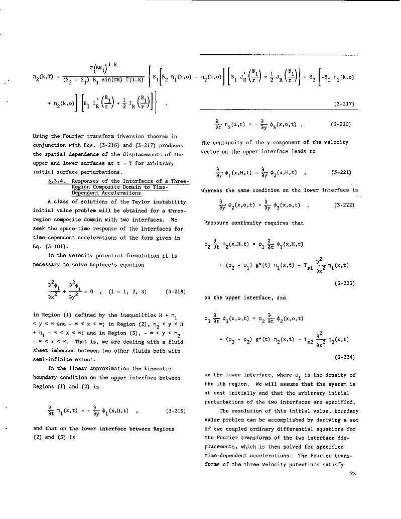
Using the Fourier transform iriversiontheorem in
conjunctionwith Eqs. (3-216)and (3-217)produces
the spatial dependence of the displacementsof the
upper and lower surfaces at t = T for arbitrary
initial surface perturbations.
3.3.4. Responses of the Interfacesof a Three-Region Composite Domain to Time-Dependent Accelerations
A class of solutions of the Taylor instability
initial value problem will be obtained for a three-
region composite domain with two interfaces. We
seek the space-timeresponse of the interfaces for
time-dependentaccelerationsof the form given in
Eq. (3-101).
In the velocity potential formulation it is
necessary to solve Laplace!s equation
a20 a20i i—+—= o,
ax2 ayz
in Region (1) defined by
< y < coand - - < x < m;
+rll- M < x < oa;and in
- -< x < m. That is, we are dealing with a fluid
sheet imbedded between two other fluids both with
semi-infiniteextent.
In the linear approximationthe kinematic
boundary condition on the upper interface between
Regions (1) and (2) is
(i= 1, 2, 3) (3-218)
the inequalitiesH + ql
in Region (2), rj2< y < H
Region (3), - m < y < r12
~ nl(x,t) ‘ - &l(x,H, t) , (3-219)
and that on the lower interface between Regions
(2) and (3) is
(3-217)
(3-220)
The continuity of the y-component of the velocity
vector on the upper interface leads to
(3-221)
whereas the same condition on the lower interface is
&2(x,o,t) =
Pressure continuity
*$3(W) . (3-222)
requires that
P2
on
P3
on
.L+ (P2 - PI) g*(t) nl(x,t) - Tsl ~nl(x,t)
(3-223)
the upper interface, and
& $3(x, o,t) = P2 ~ $2(x, o,t)
a2
+ (P3 - P2) g*(t) n2(x,t) - TS2 -#2(xJt)
(3-224)
the lower interface,where pi is the density of
the ith region. We will assume that the system is
at rest initially and that the arbitrary initial
perturbationsof the two interfaces are specified.
The resolution of this initial value, boundary
value problem can be accomplishedby deriving a set
of two coupled ordinary differential equations for
the Fourier transforms of the two interface dis-
placements, which is then solved for specified
time-dependentaccelerations. The Fourier trans-
forms of the three velocity potentials satisfy
25

~z
~ $i(k,y>t) - k2 $i(k,y,t) = O , (i = 1, 2, 3) .ay
and
~Akt =p2P33t 4(J)
To ensure
solutions
(3-225)
bounded solutions at infinity we take
of these equations as
$l(k,y,t) =A1(k,t)=ky , (3-226]
‘ky + A3(k,t) e ,ky
$Z(k,y,t) ‘A2(k,t) e (3-227)
and
$3(k,y,t) =A4(k,t) eky . (3-228)
The conditions that the y-componentof the velocity
vector be continuous on the two interfaces lead to
Al(k,t] e-kli -Idi= A2(k,t) e - A3(k,tJ eM (3-229)
and
A4(k,t) = - A2(k,t) + A3(k,t) . (3-230)
When differentiatedwith respect to time the kine-
matic conditions on the two interfacesreduce to
~2~nl(k,t) = k ~A1(k, t) e-w (3-231)at
and
a2---&2(k,t) = - k &A4(k, t) . (3-232)
Also, the interfacepressure continuity conditions
become
PI ~A1(k, t) e-HI
[‘A kt e-~= P2 at 2( , )
][+ ~A3(k, t) eW - (p2 - pl) g*(t)
*T k2S1 I
nl(k,t)
&A2(k, t) +& A3(k,t)
[+ (P3 - P2) g*(t) + Ts2 k21n2(ht). (3-234)
Solving Eqs. (3-229) and (3-230) forA2 and A3 and
entering the results into Eqs. (3-233)and (3-234)
produces
+ 2~A4(k, t)H- (P2 - PI) g*(t)
+TS1 1k2nl(kst),
where A . - 2 sinh(ldi)ando
P2
[
-kH~Ap3&A4(k.tl =% z e at ~(k,t)
(3-23S)
kH -kH a+ (e +e ) —A Hat~(k>t)+(P3 - P2) g*(t)
+T k2S2 1nz(k,t) . (3-236)
Resolving these last two relations for Alt and A4t
and combining the results with Eqs. (3-231) and
(3-232)gives a set of two ordinary differential
equations for the Fourier transformsof the dis-
placements of the two interfaces. This set reads
as follows:
a2
[---#l (k,t) + & P3 - P2
o
- (L32+ P3) e-2kHHW2-PI) ii*(t)
31 *P2+ Tsk ~l(k,t) -r
[k(p3 - P2) g*(t)
o
.
(3-233)+T
1k3 e-Mq2(k,t)=0
S* (3-237]
26

and
2p2 e-kH
DAO [ 1(P2-PI)R“(t)+T~lk3nl(k,t)32
+— z n2(k,t) -~[pl + p2
at o
H- (PI - P2) e-2w (P3 - P2) kg*(t)
+T k’S2 1
~2(k,t) = O . (3-238)
In these last two differentialequations we use the
definition
D= 1
[cjP3 e‘mA~+p2e
ldi~ ( )
,+[2kH2
o
- 4p~ e-kH - (PI + P3) P2 A.(1+ ‘=-2M)I.
(3-239)
Solutions ofEqs. (3-237)and (3-238) canbe
obtained by a method similar to that used for Eqs.
(3-192)and (3-193). The procedure now discussed
will be more general than that used previously in
that it is applicable to all forms of time-dependent
accelerations.
Obtaining solutions ofEqs. (3-237) and
(3-238)for arbitrarilyspecified time-dependent
accelerationscan be reduced to finding the solu-
tions for simpler differentialequations for the
basis functions in terms of which the solutions of
these equations can be expressed. Let the func-
tions F1 and F2 be two linearly independentsolu-
tions of
2q+v 2 kg*(t) F = O ,dt
(3-240)
and let G1 and G2 be two linearly independentsolu-
tions of
d2G—-v2kg*(t)G=0 .dt2
(3-241)
Let Ci, i = 1, 2, 3, and 4 be four arbitrary con-
stants; then the general ~olution of Eqs. (3-237)
and (3-238) in vanishing surface tensions can be
written in the form
F+c2F2+c3G1+c4G2nl(k, t) = c1 ~
(3-242)
and
[ II 1~2(k,t) = S1 Cl F1 + C2 F2 + S2 C3 G1 + C4 G2 ,
provided that the following
fied. The constant U2 is a
(3-243]
conditions are satis-
root of the quadratic
II$ [P3 - P2) PI + P2 - (Pl - P2) e-2w]
I-(P2-P1) P3-P2-
(P2 - PI) (P3 - P2)
(DA)2
[+P3-P2-(P2+133)
(p2 + p3) e-2m1}
I4P; e
-2kH
e-2kHH
PI + P2
II- (Pl - P2) e-2m = O . (3-244)
9The constant V- is a root of the quadratic obtained
from Eq. (3-244)by replacing U2 with -V2. The
constant S1 is given by either
-2kH- P2DA + (P2 - PI) P3 - P2 - (P2 + P3) e
S1 = 1
2P2 (P3 - p2) e-Idi
(3-245)
or
27
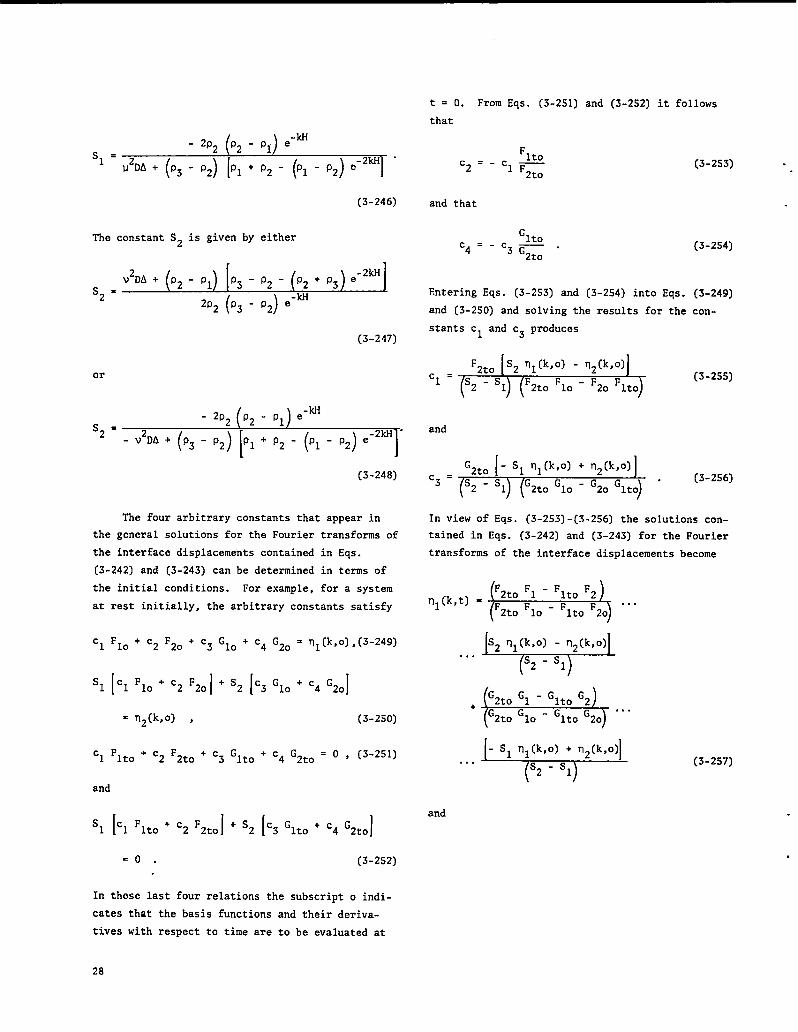
t=o. From Eqs. (3-2S1)and (3-2S2) it follows
that
- 2p2e-loll
P.2- PiS1 =
l’2DA+ (“3 -%) [PI+ ‘2 - (P1 -%) ‘-’WI “
(3-246)
The constant S2 is given by either
V2DA + p2 - “1 P3-P2-P2+P3~-2kH
S2 =2P2 (P3 - P2
)
~-ldi
(3-247)
or
- 2p2 “2 - PIe-kii
S2 =
(V2DA + P3 - P2
)[PI + “2
- h -‘4 ‘-2W]”
(3-248)
The four arbitrary constants that appear in
the general solutions for the Fourier transforms of
the interface displacementscontained in Eqs.
(3-242)and (3-243) canbe determined in terms of
the initial conditions. For example, for a system
at rest initially, the arbitrary constants satisfy
c1 ‘lo + C2 ’20 + C3 ‘%0 + C4 G20 = l(k’ol’(s-zdg)
‘1 [c1 ‘lo +C2‘d+‘2IC3‘,0+C4’201
= n2(k,o) >
c1 ‘lto + C2 ‘2to
and
(3-250)
+ C3 ‘lto + C4 ‘2to = 0 ‘ (3-251)
‘1 [c1 ‘lto + C2 F2to1[+SCG
2 3 lto + C4 ‘2toI
=0. (3-252)
In these last four relations the subscript o indi-
cates that the basis functions and their deriva-
tives with respect to time are to be evaluated at
Flto
‘2 = - c1 F2to
and that
‘ltoC4 = -c3~ “
(3-253)
(3-254)
Entering Eqs. (3-253) and (3-254) into Eqs. (3-249)
and (3-2S0) and solving the results for the con-
stants c~ and C3 produces
c1 =
and
C3 =
T%k==% (3-255)
~ ‘3-2”)
In view of Eqs. (3-253)-(3-256)the solutions con-
tained in Eqs. (3-242) and (3-243) for the Fourier
transforms of the interface displacementsbecome
‘1(’*’)=- -. . .
+
. . .
and
www (3-257)
28

half-spaces of viscous fluids. Both the stream
(F2to ‘1 - ‘lto ‘2)
L
. . .
+
. . .
The
n.(k,t) = ;I
2to Flo-F
...lto ’20
S1 S2 ~l(k,o) - n2(k,o)
52 - 51
H‘2 I
- 51 ~l(k,o) + n2(k,o)1.
52 - 51)
(3-258)
results obtained in these last two rela-
tions are valid regardless of the actual time var-
iations of the acceleration. For each particular
functional dependence of the accelerationupon time,
the basis functions required for the solutions
found in Eqs. (3-257)and (3-258) are determined as
solutions of Eqs. (3-240)and (3-241). Explicit
results for the basis functions are included in
Table 1 for both constant accelerationsand for
time-dependent
Eq. (3-101).
4. SOLUTIONS
accelerationsof the form given in
OF TAYLOR INSTABILITY INITIAL VALUEPROBLEMS FOR VISCOUS FLUIDS
Solutions of the Taylor instabilityinitial
value problems are worked out for half-spacesof a
viscous fluid, sheets of viscous fluids, and double
function and the EN formulationsdiscussed in Sec.
2 are used to solve these problems.
4.1. Solutions for a Half-Space ConfigurationwithConstant Acceleration
4.1.1. Application of the Stream FunctionFormulation
As shown in Sec. 2.1 we want to solve
P~v2$ = PV2V2$ D (4-1)
subject to appropriateboundary, kinematic, and
initial conditions. In the linear approximation
the kinematic condition on the surface of a half-
space taken as the lower half-plane becomes
~n(x,t) = -&$(x, o,t) . (4-2)
Boundary conditions to be satisfied on the
interface arise from the components of the stress
tensor. For a fluid that occupies the lower half-
plane the T -component of the stress tensor satis-YY
fies
on the surface, and the Tyx-component satisfies
‘yx =o. (4-4)
TABLEI
BASIS FONCTIONSFOR VARIOUS ACCELERATIONS
FomIof theAcceleration ‘1 ‘2 ‘1 ‘2
g*(t)= go cos[~tK@ sin(ut@) cosh(vt~) sinh(vt~)
with?= l-$ withT= l-~ withT = 1 - ~
29

Entering the expressionsfor the components of
stress tensor into Eqs. (4-3) and (4-4) yields
~zTs ~ (x,t)
av-p+zu~
“div;=]*
the
,
(4-s)
where p and A are the viscosity coefficients,and
(4-6)
Upon setting the arbitrary function of time equal
to zero in the pressure field expressionsof Eq.
(2-19) and assuming an incompressiblefluid so that
div ~ = O in Eq. (4-5),we find upon combining
these two equations in the linear approximation
that
32
[
a3—y(x, o,t] -
p atax Pg* n(x, t) + P —axay
.2 $(x, o,t)
33-—
ax 1s$(x,o,t] = o (4-7)
is the linear boundary condition that comes out of
the T -component of the stress tensor for zeroYY
surface tension. Also, Eq. (4-6) becomes
33fux,o,t) = axzay— $(x,o,t)ay3
(4-8)
in the linear approximation.
To solve the boundary value problem defined
by Eqs. (4-l), (4-2), (4-7), and (4-8) we introduce
the Laplace-Fourier
~.
$(k,y,s) = I
transform
Jw
dt e-st dx eikx $(x,y,t) .
-m
(4-9)
Let v = p/p be the kinematic viscosity; then the
Laplace-Fburiertransform of Eqs. (4-l), (4-2),
(4-7), and (4-8) for a system at rest initially
produces the following relations:
+ (k4+$) $(k,y,s) = O , (4-lo) -
S n(k,s) - ~(k,o) = ik~~(k,o,s) ,dy
(4-11)
(iks/v)$(k,o,s) + (g*/v) rl(k,s) + ik~$(k,o, s)dy
+ ik3 $(k,o,s) = O , (4-12)
and
~~(k,o,x) =-kz$v(k,o,s) . (4-13)dy
The fourth-orderordinary differentialequa-
tion that appears in Eq. (4-10) is of the so-called
Orr-Sommerfeldtype. Its general solution can be
written as
~(k,y,s) =
A3(k,s) exp(-kyl + A4(k,sl exp(-y=~).(4-14)
For a half-space in the
A3 = O = A4 for bounded
write
$(k,y,s)=A1(k,s) I#y
with
lower half-plane we take
solutions at infinity and
+ A2(k,s) e’y (4-15)
(4-16)
At this point three quantities,namely, Al(k,s)
and A2(k,s) in Eq. (4-15) and ~(k,s) remain to be .
found. Entering Eq. (4-15) into Eqs. (4-11)-(4-13)
gives three algebraic equations for their determina-
tion. It follows from Eq. (14-13) that
30

4.1.2. Application of the DNS Formulation
A2(k,s) = z- 2k3
~ ~ + ~3 Al(k,s) >
and Eqs. (4-11) and (4-12)become
(4-17)
s n(k, s) - q(k,o) = (ik) [k A1(k,s) + K A2(k,s)I(4-18)
and
{( )[(g*/v) n(k,s) = (- ik) $+ kz Al(k,s) + A2(k,s)1.1+k2 Al(k,s) + K2 A2(k,s) . (4-19)
Upon resolving Eqs. (4-17)-(4-19)the Laplace-
Fourier transform of the interfacedisplacementis
found to be given by
rl(k,s)rl(k,o)
(4-20)
Also, the Laplace-Fouriertransform of the partial
derivativeof the interface displacementwith re-
spect to time is
-S n(k, s) - n(k,o)
->g * ~(k,o)
7 2 . (4-21)
k4 r]-41+ L+?vk2
The space-timeresponse of the interface dis-
placement and its time derivative can be determined
from Eqs. (4-20) and (4-21)by using the inversion
theorems for Laplace and Fourier transforms. How-
ever, before considering this aspect of the problem
we shall discuss the applicationof the DNS formula-
tion presented in Sec. 2.3 to this same problem.
As indicated in Sec. 2.3 the DNS formulation
provides a unified approach for the treatment of
Taylor instabilityinitial value problems for both
viscous and inviscid fluids. In contrast to the
stream function method of Sec. 4.1.1, where it was
necessary to solve a fourth-orderdifferential
equation, only second-orderdifferentialequations
need to be solved in the DNS formulation. We now
demonstratee this for the half-space problem.
We start from the complex Fourier
ofEqs. (2-57) and (2-59),which are
~z~P(k,y,t) - kz P(k,y,t) = O ,ay’
~u(k, y,t)= &P(k,y,t) + V
transforms
(4-22)
.L
~ u(k,y,t)ay
1-kz u(k,y,t) , (4-23)
and
[
32&v(k, y,t)= - ~~ P(k,y,t) + V ~v(k, y,t)
ay
1-kz v(k,y,t) . (4-24)
The solution of Eq. (4-22) of interest for the
lower half-spaceproblem is
P(k,y,t) =A1(k,t)eky , (4-25)
with which Eqs. (4-23) and (4-24) become
a
[
32~ u(k,y,t) = &Al(k, t) eky+vnu(k, y,t)
ay
- k2 u(k,y,t)1and
~v(k, y,t) = - LA (k,t) e
[
ky+vazpl
~ v(k,y,t)ay
1-k2 v(k,y,t) . (4-27)
31
(4-26)

In this formulationthe kinematic condition on
the interface is used in the form
+ rl(x,t) = V(x,o,t) , (4-28)
the boundary condition from the T -componentYY
the stress tensor is
P(x,o,t) - Pg* rl(x, t) - 2P* V(x,o,t) = o ,
of
(4-29)
and the boundary condition from the ‘r -componentyx
of the stress tensor is
&@jt) + ~v(x, o,t). IJ . (4-30)
The Laplace transformsof the complex Fourier
transforms of the x- and y. componentsof the line-
arized Navier-Stokes equations obtained from Eqs.
(4-26) and (4-27) are
S u(k,y,s) - u(k,y,o) = #A1(k, s) eky
[
32+ V ~u(k,y,s) - k2 u(k,y,s)
ay 1and
S v(k,y,s) - v(k,y,o) =
[
a2+v— v(k,y,s] -
ay2
If the fluid is at rest
-~A1(k,s) eky
1
k2 v(k,y,s) .
initially,then
(4-31)
(4-32)
Eqs. (4-31)
and (4-32) reduce to the following one-dimensional,
inhomogeneousscalar Helmholtz equations for the
Laplace-Fouriertransforms of the x- and y-compo-
nents of the velocity vector;
a2~u(k, y,s) -
(:+
ay
=-~Akpv 1( ,s)
k2)u(k,y,s)
kye (4-33)
a2
();+k
2~v(k,y,s) - v(k,y,s) =
ky~A1(k,s) e .
ay
(4-34)
With the quantity K, as defined in Eq. (4-16), the
solutions of Eqs. (4-33) and (4-34) appropriate for
a half-space in the lower half-plane are
u(k,y,s) = Cl(k,s) eKy + $$ Al(k,s] eky (4-3s)
and
v(k,y,s) = C3(k,s) eKy ky- &A1(k, s) e . (4-36)
The quantities Cl, C3, and Al in these last
two equations are found by satisfying the Laplace-
Fourier transforms of the kinematic and boundary
conditions, together with that of the continuity
equation,which is
&v(k, y,s) = i k u(k,y,s) . (4-37)
Upon entering Eqs. (4-35) and (4-36), this relation
leads to
C3(k,s) = (ik/K)Cl(k,s] . (4-38)
The Laplace-Fouriertransforms of the kinematic and
boundary conditions read
A1(k,s) = P(k,o,s) = pg’ V(k,s) + 2u~ay v(k, o,s) ,
(4-39)
&u(k,o,s) = ik v(k,o,s) , (4-40)
and
S rl(k,s) -
These last
~(k,o) = v(k,o,s) .
three equations become
(4-41)
and
32

[k2 1 In this result
Al(k,s) = pg’ q(k,s) + 2V K C3(k,s) - ~Al(k,s) , 4 are the four
the quantities qi,
roots of
(4-42) A 7
2
[K Cl(k,s) + ~A1(k, s) = (ik) C3(k,s)
1-;Al(k,s) , (4-43)
L A J.V’ k=
and the denominator is the cubic
( )D’(qi)=4q;+qi-l .
andTo establish Eq. (4-45) from
following procedure can be used.
s n(k,s) = n(k,o) + C3(k,s) - ~A1(k,s) . (4-44) right-hand side of Eq. (4-21) as
The sameresult for the Laplace-Fouriertransform
of the interfacedisplacementas that quoted in V(k,o) (-k/v2)g*.
i = 1, 2, 3, and
o, (4-46)
(4-47)
Eq. (4-21) the
First write the
—.
(4-42)-(4-44).
4.1.3. Inversion of the Laplace Transform
In Sees. 4.1.1 and 4.1.2 the stream function To find
and the DNS formulationswere used to determine inverse
Eq. (4-20) is obtained by solving Eqs. (4-38) andw$~x+~
the inverse of this expressionmultiply the
of the following expressionsby exp(-tvk2);
rl(k,o)(-k/v2)g*
m
= q(k,o) - \
.!! ?&+!%
.2 G .’3
( v ‘w(vk2) [(~+ l);- 4@+fi] “
(4-48)
the Laplace-Fouriertransform of the displacement We now invert the following quantity and replace t
of the surface of a half-space of a viscous fluid 2with vk t in the result
subjected to a time-independentacceleration. Also,
the Laplace-Fouriertransform of the time derivative
()rl(k,o) - ~ A
of the surface perturbation is given by Eq. (4-21).V2 k4 (S+l)2-:6+fi “
If this equation is inverted back into the time
domain, the time derivative of the Fourier transform
of the surface displacementis found to be
~ ~ e“k2t(~-1)erfc(- qi~) .&rl(k,t) =rl(k,o) (-~) ~~
i=l qi
(4-45)
33
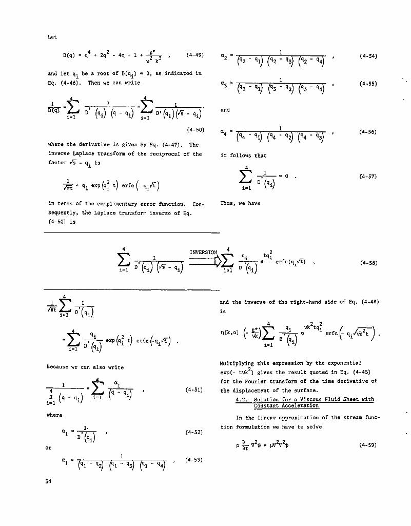
Let
D(q) = q4 + 2q2
let qi be a root
(4-46). Then we
4q+l+L~2 ~3 ‘
(4-49)
of D(qi) = 0, as indicated in
can write
1‘2 =
)(qz-ql qz-q~ qz-qo ‘
)
(4-54)
and
Eq. 1‘3 = q~ - ql qs - qz
)q~-q4 ‘
(4-55)
1~= 2
i=l i (qi;(q-‘J ‘f+’”(qi;(& - qi)’and
1a4 = ’14
)(- q~ q4 - qz q4-q3 ‘
(4-S6)(4-50)
where the derivative is given by Eq. (4-47). The
inverse Laplace transform of the reciprocal of the
factor & - qi isit follows that
2 1- .0.
()D qi
i=l
(4-57)1
~+qi “p (“ ‘) ‘rfc(- ‘ifi)
in terms of the complimentaryerror function. Con-
sequently, the Laplace transform inverse of Eq.
(4-S0] is
l%us, we have
.q- tq;
~ e
()
erfc(qifi) ,D qi
(4-58)
and the inverse of the right-hand side of Eq. (4-48)
is
qi—e
()D’ qi‘k2t{ erfcf qi=~ .
i=1
Multiplying this expressionby the exponential
exp(- tvk2) gives the result quoted in Eq. (4-4S)
for the Fourier transform of the time derivative of
Because we can also w-rite
(4-51) the displacementof the surface.
4.2. Solution for a Viscous Fluid Sheet withConstant Acceleration
In the linear approximationof the stream func-where
tion formulationwe have to solve.
1-.- ,‘1
()D qi
or
(4-52)
I+& @v21$ (4-s9)
1al = ql - q2 ql - qs q~ - qo ‘
(4-53)
34

to determine the space-timeresponse of the upper
and lower surfaces of a viscous fluid sheet. The
pressure field can be written as
on the lower surface and to
. 32p(x,y,t) = p. + p~$(x,y,t) - pg’y
[v ~ ~(x,H,t) - ~
axay~ V(x,H, t) 1 (4-66)
of the[
a3 a3-v --#(x,y,t) + —
axay2 w(xsY,t.)1
+
on the
stress
(4-60)
upper surface. The T -componentyx
tensor becomesand
a2p(x, y,t) = PH + P =V(x>y, t) - pg*(y - H) 33 33
--7j*(x.o,t) = — W(x,o,t)ay ax2ay
(4-67)
[
a3 a3-u -&(x, y,t) + — 1~iJ(x,Y,t) . (4-61)
axayon the lower surface and
In Eq. (4-60) the pressure at the mean position of
the lower surface is po, and pH is the pressure at
the mean position of the upper surface in Eq.
(4-61). With these two expressionsfor the pres-
sure field it is possible to put the T -componentYY
of the stress tensor for an incompressiblefluid,
namely,
a3 a3~ V(x,H,t) = — $(x,H,t)ay ax2ay
(4-68)
on the supper surface.
The solution of Eq. (4-59), subject
kinematic and bcundary conditions of Eqs.
to the
(4-63)-
(4-68), can be determined by the method of multi-
ple integral transforms. We use a Laplace transform
on the time coordinate and a complex Fourier trans-
form on the x-coordinate,namely,
(4-62)
into two alternative forms that can be used in the
boundary conditions on the upper and lower surfaces
of the fluid sheet.
The kinematic condition on the upper surface
at y = H + ~l(x,t) is
~(k,y,s)‘Jmdte-st[ ‘k ‘kxv(x$yst) o “-69)o
The Laplace-Fouriertransform of Eq. (4-S9) is
a2~ rll(x,t)= v(x,H,t) = - ~$(x,H, t) , (4-63)
and that on the lower surface at y = ~2(x,t) is
d4-@k,y,s) - (:+ 2k2) ~v[k,y,s)
+k()
2 k2+; $(k,y,s) = O . (4-70).L
&12(x,t) = V(x,o,t) = - & V(x,o,t) , (4-64)
The general solution of this equation is
both in the linear approximation. The T -componentYY
of the stress tensor leads to the boundary condi-
tion
$(k,y,s) = Al(k,s) ~y + A2(k,s) e_ky + A3(k,s] e!y
- Ky+ A4(k,s) e , (4-71)
.Q(x,o,t) = g*T12(x,t)
where K2 = k2 + s/V.
[
a3 a3+V -#$(x’o’t) - — 2 V(x,o,t)1 (4-6S)
axay
35
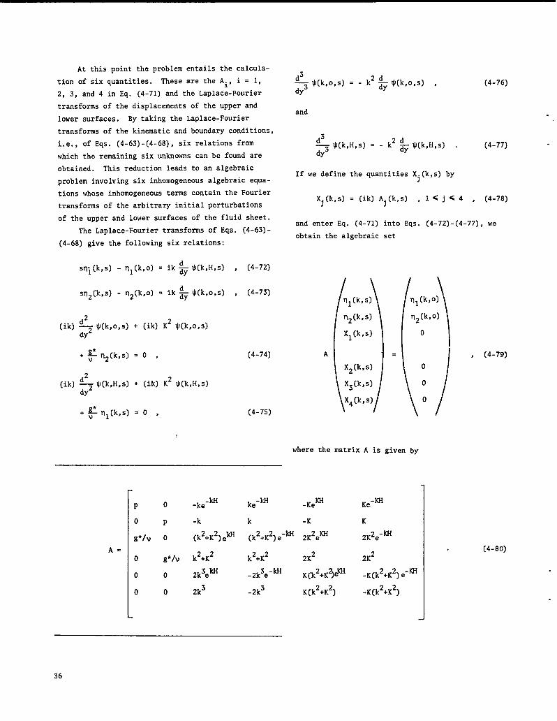
At this point the problem entails the calcula-
tion of six quantities. These are the Ai, i = 1,
2, 3, and 4 in Eq. (4-71) and the Laplace-Fourier
transformsof the displacementsof the upper and
lower surfaces. By taking the Laplace-Fourier
transformsof the kinematic and boundary conditions,
i.e., of F!qs.(4-63)-(4-68),six relations from
which the remaining six unknowns can be found are
obtained. This reduction leads to an algebraic
problem involving six inhomogeneousalgebraic equa-
tions whose inhomogeneousterms contain the Fourier
transformsof the arbitrary initial perturbations
of the upper and lower surfaces of the fluid sheet.
The Laplace-Fouriertransforms of Eqs. (4-63)-
(4-68) give the following six relations:
s~i(k,s) - ~l(k,o) = ik $$(k, H,s)
sq2(k,s) - q2(k,o) = ik ~ $(k,o,s)dy
(ik)$ ~(k,o,sl + (ik) K2 $(k,o,s)dy
&2(k,s) = O ,‘v
(ik)< ~(k,,,s) + (ik) K2 $(k,H,s)dy
+$rll(k,s) = O ,
, (4-72)
, (4-73)
(4-74)
(4-75)
A=
+ ~(k,o,s) = - k2$~(k,o,s) ,dy
and
(4-76)
(4-77)
If we define the quantities Xj(k,s) by
Xj(k,s) = (ik) Aj(k,s) , 1 s j s 4 , (4-78)
and enter Eq. (4-71) into Eqs. (4-72)-(4-77),we
obtain the algebraic set
A
Nnl(k,s)
n2(Ls)
Xl(k,s)
X2(k,s)
\
X3(k,s)
x4(k,s)
/
.
where the matrix A is given by
P o -ke-Idi
kc-w
o P -k k
-KeKH
-K
g*/v o ~k2+K21ekH ~k2+K21e-kH 2K2eKH
ok2+K2
g*/vk2+K2
2K2
o 0~k3ekH -2k3e-kH
K(k2+K~~
o 0 2k3 -2k3 K(k2+K2)
Kc-m
K
2K2e-KH
2K2
-K(k2+K2)e-M
-K(k2+K2)
, (4-79)
(4-80)
36

The solutions of Eq. (4-79) for the Laplace-
Fourier transform of the displacementof the upper
surface of the fluid sheet can be written in the
form
nl(ko) 1 ~ T31(k>s)s ~ll(k,s) + $M31(k>s) - n2(k,o) “~l(k,s) =
()~2 D31(k,s) + s$[631(k,s) -&ll(k,s)s2 + “ 1
D21(k,s)
The determinantsin this result are defined by the
relations that follow:
611(k,s) =
M31(k,s) =
T31(k,s) =
D31(k,s) =
(k2+K2)eM (k2+K2)e-M 2K2ew ~.2e-KJ3
k2+K2 ~2+K22K2 2K2
*k3ekH -2k3e-kHK(k2+K2)eW -K(k2+K2)e-w
2k3 -2k3 K(k2+K2) -K(k2+K2)
-k k -K K
(k2+K2)em (k2+K2)e-w 2K2e~ ~K2e-KH
2k3ekH -2k3e-kHK(k2+K2)em -K(k2+K2)e-KH
2k3 -2k3 K(k2+K2) -K(k2+K2)
-keM ke-kH-Kern Kc-m
(k2+K2)ew (k2+K2)e-w 2K2~m *K2e-KH
~k3ekH -2k3e-kH K(k2+K2)ew -K(k2+K2)e-m
2k3 -2k3 K(k2+K2) -K(k2+K2)
(4-81)
(4-82)
(4-83)
(4-84)
-Icew ~ -kH -icew ~-iai
-k k -K K
*2k3eldi -2k3e-kH 22KH
K(k +K ]e -K(k2+K2)e-m
2k3 -2k3 K(k2+K2) -K(k2+K2)
(4-85]
37

-k k -K K
(k*+K*)ew (k2+K2)e-w 2K2=W*K2e-KH
631(k,s) = s~k3ekH -2k3e-kH
K(k2+K2)em -K(k2+K2)e-m
2k3 -2k3 K(k2+K2) -K(k2+K2)
and
D21(k,s) =
A property of these si
-ke~ ~-ldi-Kew
~-la-l
k2+K2 k2+K22K2 2K2
2k3ekii -2k3e-kH 22KHK(k +K )e -K(k2+K2)e-~
2k3 -2k3 K(k2+K2) -K(k2+K2)
determinantsto be used
later is that they are all odd functions in the
Fourier transformvariable k, that is,
~ll(-k,s) = - 611(k,s) , (4-88)
M31(-k>s) = - M31(k,s) , (4-89)
T31(-k,s) = - T31(k,s) , (4-90)
D31(-k>s) = - D31(k,s) , (4-91)
631(-k,s) = - cS31(k,s) , (4-92)
and
D21(-k,s) = - D21(k,s) . (4-93)
The space-timeresponse of the displacementof
the upper surface can now be computed with the in-
version theorems for Laplace and complex Fourier
transforms. We obtain directly the integral rep-
resentation
nl(x,t) =&~-dkCixk&~i=dsZs~l[k,s]
..CO c-ire(4-94)
where rll(k,s)is given by Eq. (4-81).
(4-86)
.
(4-87)
As an explicit example of this general result
for arbitrary initial perturbationson both surfaces
of the fluid sheet, consider initial cosine pertur-
bations on each surface with a phase difference c.
That is, suppose that the initial displacementson
the upper and lower surfaces are given by
and
The
nl(x,o) = al cos(kox + s)
n2(x,o) = a2 cos(kox) .
complex Fourier transforms
(4-95)
(4-96)
of these initial dis-
placements are
nl(k,o) [=male ‘c 6(k+ko) + e-ie 6(k-ko)] (4-97)
n2(Lo) = m a2~(k+ko) + &(k-ko)] . (4-98)
Upon combining Eqs. (4-81), (4-94), (4-97),and
(4-98),carrying out the integrationover the
Fourier transform variable k, with the use of the
shifting property of the Dirac delta function, and
making use of the odd properties of the fourth-
order determinants expressed in Eqs. (4-88)-(4-93),
.
38

we find that the space-timeresponse of the upper
surface of the fluid sheet can be representedby
the Bromwich integral
for each of the two regions, we find that the conti-
nuity of the T -component of the stress tensor onYY
the interface leads to the boundary condition
~z—$ (X,o,t) - Pig’ n(x,t)
‘I atax I\
c.+ic.anl(x, t) = ~
ds ets
I6(ko, s) al
cos(kox+s) . . .
c-irn
.
83 83--@(x,o, t) + PI ~ $l(xDoyt)
axay- PI
. p2
- ?J2
. . . IS ~ll(ko,s)+~M31(ko,d]
- az cos(kox)$T31(ko,s) I.
azatax ~~(x,o,t) - P2 g* ll(Xlt)
83 83&2(x,o,t) + ?-12—
axayz
(4-99)
IJz(x,o,t) ,
in the complex s-plane. Here we have introduced
the definition(4-104)
in the absence of surface tension.
of the T -component of the stressyx
the boundary condition
The continuity
tensor leads to[6(ko,s) = 611(ko,s) S2 + ~ d31(ko,s)
-D21(kos)l+($rD31(ko,s) o (4-100)1
[
83 83PI ~ Vl(x$o,t) - —$l(x,o,t)
ay axzay 14.3. InterfaceMotion between Two Half-Spacesof Incompressible,Viscous Fluids under Con-stant Acceleration
To determine the space-timeresponse of the
83 83~vz(x,o,t) 1-—qJ2(x,o,t) .ay axzay
interfacebetween two viscous fluids under constant
accelerationwe solve the two uncoupled partial (4-105)
differentialequations of the stream function for-
mulation in the linear approximation. In Region The continuity of the x-component of the velocity
vector requires that(l), defined by the inequalities-CO< x c @ and
y B o, we have
(4-106)~ V2‘1 at
and in Region
~ V2‘2 at
The interface
(4-101)
y < 0, we have
(4-102)
is
(4-103)
(2), -@<x<@and and that of the y-component of the velocity vector
gives the boundary condition
+2=P2V%2Q2 .82 82
~ @l(x, oDt).Wljz(x,o,t) . (4-107)kinematic condition
To solve the initial value, boundary value
problem representedby Eqs. (4-101)-(4-107)we in-
troduce the Laplace-Fouriertransforms of the scalar
functions vi, defined by.
.
The four required boundary conditions for this
problem arise from the continuity of the T - andYY
-componentsof the stress tensor and the conti-‘yxnuity of the x- and y-componentsof the velocity
vector. By using pressure field expressionsof the
form given in Eq. (4-60) and stress tensor compo-
nent expressionsof the form given in Eq. (4-62]
39
[
m
$i(k,y,s) = dt e-st ...
0
/
Co*
dx eikx
... $i(x,y,t), (i=l,2) ,
..W
and of the interface displacementby
(4-108)
(4-109)
For y > 0, the Laplace-Fouriertransform of Eq.
(4-101) is
+k’kz+
(
and for y c o,
)& ~l(k,y,s) = O ,1
that of Eq. (4-102) is
+ *z[k,y,sl
- (’k’+35“’k’y$s’‘y +k2(k’+~)$2(k,y,s] =0.
To ensure bounded solutions at infinity we
solution of Eq. (4-110) in the form
$I(k,y,s] = Al(k,s) e_ky + A2(k,s) e_K1y ,
and that of Eq. (4-111) in the form
K2y~2(k,y,s) = Bl(k,s) eky+ B2(k,s) e ,
where
K;=k2+~,i
The problem can
(i=l,2) .
(4-110)
(4-111)
take the
(4-112)
(4-113)
(4:114)
now be reduced to a set of
in Eq. (4-113),and ~(k,s), the Laplace-Fourier
transform of the interface displacement. To accom-
plish this reduction we first take the Laplace-
Fourier transforms of the kinematic and boundary
conditions given in Eqs. (4-103)-(4-107). These
five transformsread as follows:
s n(k,s) - n[k,o) = (ik)&J1(k,o,s) , (4-11s)
PI sik Vl(k,o,s) + PI g* ~(k,s) + PI ik3 ~l(k,o,s)
+ PI i+$l(’,%d =P2 sik $Z(k>o,s)ay
+ P2 g* n(k,s) + !.12ik3 $Z(k,o,s)
(4-116)
[
33
~1 ~V1(k,o,s) + ‘ay
‘&$l(k,o,s) 1[.33. p2 2a~$2(k,o,s) + ‘ay 1~V2(koA,(4-117)
32 32~lj(k,o,s)ay
= ~$2(’,o,s) ,ay
(4-118)
and
; Vl(ko)s) ‘$42(LOA . (4-119)
Upon entering Eqs.
(4-116)-[4-119)we
(4-112) and (4-113) into Eqs.
find that
Av
(
)Al(k,s)
A2(k,s)
.
Bl(k,s)
B (k$s)\2
/(Pl - P2)
(-ik)
)
g* n(k,s)
o
0
{0
where the matrix Av is given by
(4-120)
five inhomogeneousalgebraic equations in which the
unknowns are Al and A2 in Eq. (4-112),B1 and B2
40

. Av =I()PI k2+K:
21@3
k
k2
Also, Eq. (4-115)becomes
K1
K:
s n(k,s) - rl(k,o) = (-ik) [kA1(k,s) + KlA2(k,s)]
Solving Eq. (4-120) for Al and A2 yields
A ,,,s, . !d!dd ,*,,,,s,1 Av (-ik)
and
A ,k,s, .- !id!?ddgk ,[k,s,2 Av (-ik)
where the two additional determinants
,
are
AV,13 ❑
and
A~,23 =
(4-122)
(4-123)
(4-124)
()-P2 k2+K: 2-2~2K2
2p2k3()2+K2‘
U2K2 k ~
k‘2
-k2 -K;
(4-121)
Combining Eqs. (4-122)-(4-124)produces
Av U(k,o)q(k,s) = sA
+ K1 Av 23 - kAv 13v P1-P2 g’
9 *
(4-127)
as the Laplace-Fouriertransform of the interface
displacement. A little algebra establishesthe
identity
K1Av23-kAv13=sA, s V,3 ‘
where
(4-128
A 2V,3 ‘kKlK2 [
PI K2 + P2 K1 - k(pl+pz)] . (4-129)
42+0 2~2k3 ~2%(k2+K:)
‘1 k‘2
K; -k2 -K:
(4-125)
k2
2~2k3 ()V2K2 k2+K~
k‘2
-k2-< “
(4-126)
41

Consequently,the Laplace-Fouriertransform of the
interfacedisplacementbecomes
n(k,s)=w A ,Av; p~p2g, , (4-130)v
and that of the time derivative of the interface
displacementis
“(k]s)-’(kJ0)~*o(4-131)By applying the inversion theorems for the
Laplace and Fourier transforms the following inte-
gral representativesfor the space-timeresponse
of the interfaceand its time derivative are ob-
tained:
ll(x,t) = ~1
dk e-ixk ~(k,o) ...
-m
c+iw
hdsAv ets
1““”= ~Av+Av
(4-132)
BC-ire
and
~n(x,t) = -+ r’dk e-ixk ~(k,o) ...
-w
For an initial cosine perturbation, for which
(4-134)
we find that
n[x,t]-a.Coskd271i ““”
and (4-135)
r+i- (P1-P2 g*Av s ko,sets
... ds Av ko,s + Av ~ ko,s P1-P2 g*#
c-i=(4-136)
are the Bromwich integral representationsof the
interface displacementand its time derivative,re-
spectively.
REFERENCES
1.
2.
3.
4.
5.
6.
7.
8.
9.
10.
11.
12.
13.
14.
Lord Rayleigh, !?Investigationof the Character
of the Equilibrium of an IncompressibleHeavyFluid of Variable Density,” Scientific Papers,Vol. 2, 200, Cambridge (1900]; also, Proc.London Math. Sot. LQ, 170 (1883).
A. G. Greenhill, IvWaveMotion in Hydrodynamics,”
Amer. J. Math. ~, 62 (1887).
W. J. Harrison, “The Influence of Viscosity onthe Oscillationsof Superposed Fluids,” Proc.London Math. Sot. Q, 396 (1908).
G. Taylor, IfTheInstabilityof Liquid Surfaceswhen Accelerated in a Direction Perpendicularto their Planes. I,” Proc. Roy. Sot. A 2&, 192(1950).
D. J. Lewis, !lfieInstabilityof Liquid Surfaces
when Accelerated in a Direction Perpendiculartotheir Planes. 11,” Proc. Roy. SOC. A, ~, 81(1950).
M. S. plesset, ~~Onthe Stability of Fluid Flows
with Spherical Symmetry,!’Rand Corporationre-port ”AECU-2997,pp. 1-9 (1953).
R. Bellman and R. H. Pennington,“Effects ofSurface Tensions and Viscosity on Taylor In-stability,”Quart. Appl. Math. ~, 151 (1954).
R. L. Tngraham, ‘!TaylorInstabilityOf the In-
terface between Superposed Fluids-SolutionbySuccessive Approximations,”Proc. London Phys.SOC. B ~, 748 (1954).
M. S. Plesset and T. P. Mitchell, “On the Sta-bility of the Spherical Shape of a Vapor Cavityin a Liquid,” Hydrodynamic Laboratory,Calif.Inst. Tech. report No. 26-9 (1954).
G, Birkhoff, ItTaylorInstabilityand LaminarMixing,!!LOS Alamos Scientific Laboratory re-
port LA-1862 (19S5);Appendixes A-H issued asreport LA-1927 (19S6).
S. Chandrasekhar,!tTheCharacter of the Equilib-rium of an IncompressibleHeavy Viscous Pluid ofVariable Density,” Proc. Cambridge Phil. Sot.~, 162 (1955).
T. Y. Teng Fan, “The Character of the Instabil-ity of an IncompressibleFluid of ConstantKinematic Viscosity and ExponentiallyVaryingDensity,” Astrophys. J. ~, 508 (195S).
R. Hide, ~!~e Character of the Equilibriumofan IncompressibleHeavy Viscous Fluid of Vari-able Density: An ApproximateTheory,” Proc.Cambridge Phil. Sot. ~, 179 (1955).
R. LeLevier, G. J. Lasher and F. Bjorklund,I?Effectof a Density Gradient on Taylor InSta-bility,!tLawrence Livermore Laboratory rePortUCRL-4459 (1955).
.
.
.
42

.
15.
16.
17.
18.
19.
20.
21.
22.
23.
24.
25.
26.
27.
28.
29.
30..
.
D. Layzer, !!Onthe InstabilityOf Superposed
Fluids in a GravitationalFluid,” Astrophys.J. ~, 1 (1955).
C. M. Tchen, “Stability of OscillationsofSuperposed Fluids,” J.-Appl. Phys. 27, 760(1956).
—
80 R. Morton, t!Onthe EquilibriumOf a Strat-
ified Layer of Fluid,” Quart. J. Mech. Appl.Math. ~, 433 (19S7).
G. F. Carrier and C. T. Chang, “On an InitialValue Problem Concerning Taylor Instabilityof IncompressibleFluids,” Quart. Appl, Math.
@ 436 (1959).
S. Feldman, “On the InstabilityTheory of theMelted Surface of an Abating Body when Enter-ing the Atmosphere,!’J. Fluid Mech. ~, 131(1959).
S. Chandrasekhar,Hydrodynamicand Hydromag-netic Stability (ClarendonPress, Oxford,1960), Chap. X, p. 428,
H. W. Emmons, C. T. Chang, and B. C. Watson,T7Taylor Instability of Finite Surface h’aVes,”
J. Fluid Mech. ~, 177 (1960).
K. M. Case, !Istability of an IdealizedAtmo-
sphere. I. Discussion of Results,” Phys. Flu-ids ~, 149 (1960).
K. M. Case, !lTaylorInstabilityof an Inverted
Atmosphere,”Phys. Fluids ~, 366 (1960).
R. D. Richtmyer, ‘fTaylorInstability in Shock
Accelerationof CompressibleFluids,” Comm.Pure and Appl. Math. ~, 297 (1960).
J. N. Hunt, l!Taylor Instabilityin a Thin
Fluid Layer,” Appl. Sci. Res, A ~, 45 (1961).
J. N. Hunt, ‘!Instabilityin a Spherical FluidShell,” Appl. Sci. Res. A~, 59 (1961).
W. H. Reid, I,TheEffects of Surface Tensions
and Viscosity on the Stability of Two Super-posed Fluids,” Proc. Cambridge Phil. Sot. ~,415 (1961).
M. Mitchner and R. K. M. Landshoff, “Rayleigh-Taylor Instabilityfor CompressibleFluids,”Phys. Fluids ~, 862 (1964).
F. Selig, !!VariationalPrinciple for Rayleigh-
Taylor Instability,”Phys. Fluids ~, 1114(1964).
I. G. Cameron and H. H. M. Pike, “InterfaceInstabilityunder Variable Normal Accelera-tion,” AWRE report No. 0-96/64 (1965).
31.
32.
33.
34.
35.
36.
37.
38.
39.
40.
41.
42.
43.
44.
45.
L. A. Elliott, *perturbationson Fluid Sur-
faces,” Proc. Roy. SOC. A2YJ, 397 (1965).
A. J. Wilson, ~~onthe Stability of TWO Super-posed Fluids,” Proc. Cambridge Phil. Sot. 61_,595, (1965).
F. H. Harlow and J. E. Welch, “Numerical Studyof Large-AmplitudeFree-SurfaceMotions,” Phys.Fluids ~, 842 (1966).
J. W. Miles, “Taylor Instabilityof a FlatPlate,” General Atomics report GAMD-7335(1966).
J. W. Miles and J. K. Dienes, “Taylor Insta-bility in a Viscous Fluid,” Phys. Fluids ~,2518 (1966).
B. J. Daly, !!NumericalStudy Of Two-Fluid
Rayleigh-TaylorInstability,”Phys. Fluids l&,297 (1967).
N. R. Rajappa, “A Non-Linear Theory of TaylorInstabilityof Superposed Fluids,” Ph.D.Thesis, Dept. Aero. Astro., Stanford Univ.(1967).
B. Jo Daly, ‘tNumericalStudy Of the Effect of
Surface Tension on Interface Instability,”Phys. Fluids ~, 1340 (1969).,
R. L. Kiang, ‘Nonlinear Theory of InviscidTaylor InstabilityNear the Cut off WaveNumber,” Phys. Fluids ~, 1333 (1969).
A. H. Nayfeh, “On the Non-Linear Lamb-Taylorln~tability,,,Jo Fluid Mech. ~, 619 (1969).
K. A. Meyer and P. J. Blewett, “Some Prelim-inary Numerical Studies of Taylor Instabilitywhich Include Effects of Material Strength,’fLos Alamos Scientific Laboratory reportLA-4754-MS (1971).
F. Troyon and R. Gruber, “Theory of the Dynam-ic Stabilizationof the Rayleigh-TaylorInsta-bility,” Phys. Fluids ~, 2069 (1971).
K. A. Meyer and P. J. Blewett, “Numerical In-vestigation of the Stability of a Shock-Accelerated Interface between Two Fluids,”Phys. Fluids ~, 753 (1972).
G. H. Pimbley, Jr., l!AnAnalysis of theRayleigh-TaylorProblem of Superposed Fluids,”Los Alamos Scientific Laboratory reportLA-4839 (1972).
J. Berg~ans, !!Stabilityof a Curved Gas-Liquid
Interface,”Phys. Fluids l&, 188 (1973).
* uSGOVWMEWPNWINQ O= CE1974–7M-5WIM
EE:202(60)
43