Introduction and Advances in Gaussian Processeschasen.org/~daiti-m/paper/svm2009advgp.pdfH(x)) Introduction and Advances in Gaussian Processes – p.4/29 GP の導入(1) • y(1) ···y(N)

Introduction and Advances in Gaussian Processes

持橋大地NTTコミュニケーション科学基礎研究所

[email protected]

SVM 2009

Modified for NTT厚木基礎研2009–10–13 (Tue)

Introduction and Advances in Gaussian Processes – p.1/29

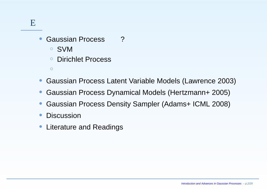
流れ

• Gaussian Processとは?◦ SVMとの関係◦ Dirichlet Processとの関係◦ 例と簡単な応用

• Gaussian Process Latent Variable Models (Lawrence 2003)• Gaussian Process Dynamical Models (Hertzmann+ 2005)• Gaussian Process Density Sampler (Adams+ ICML 2008)• Discussion• Literature and Readings


Gaussian Processとは

−8 −6 −4 −2 0 2 4 6 8−3

−2

−1

0

1

2

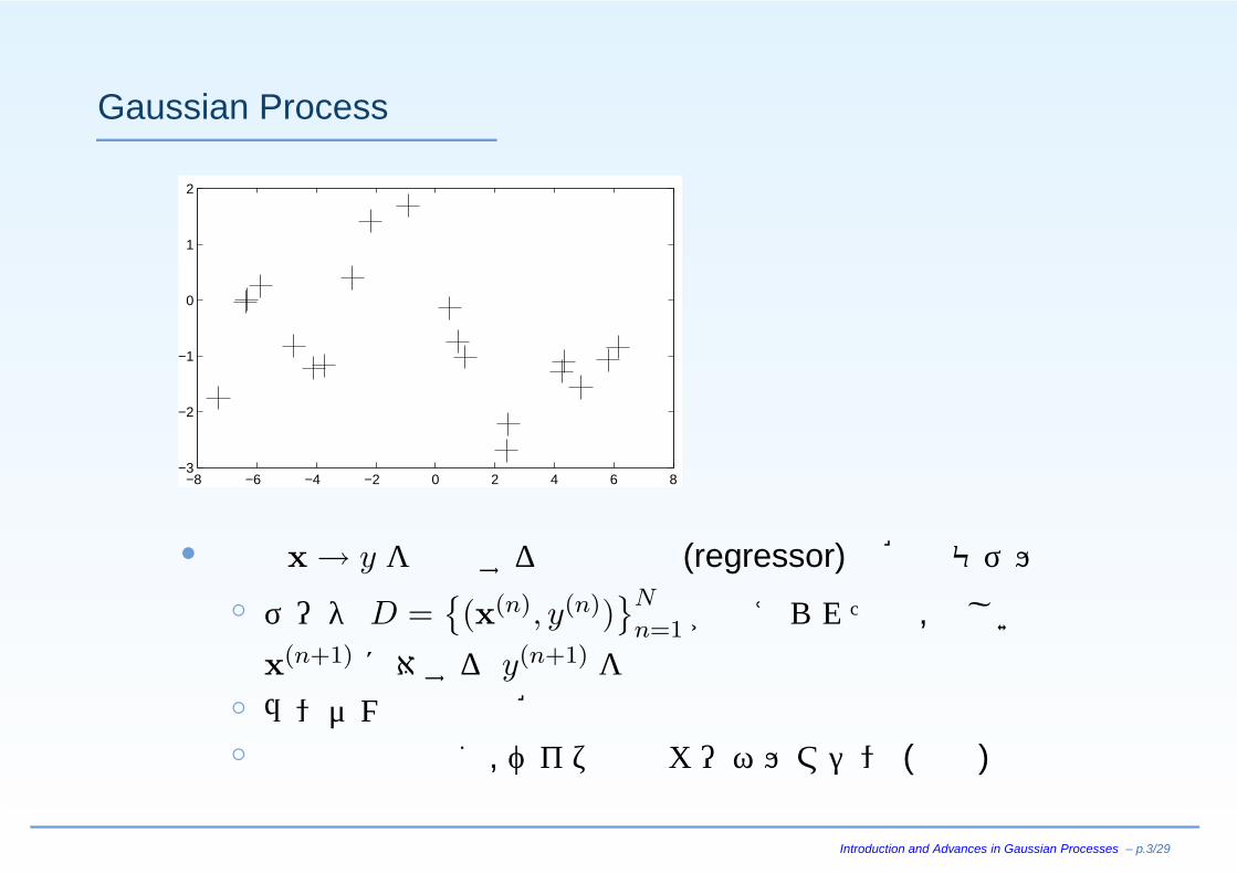
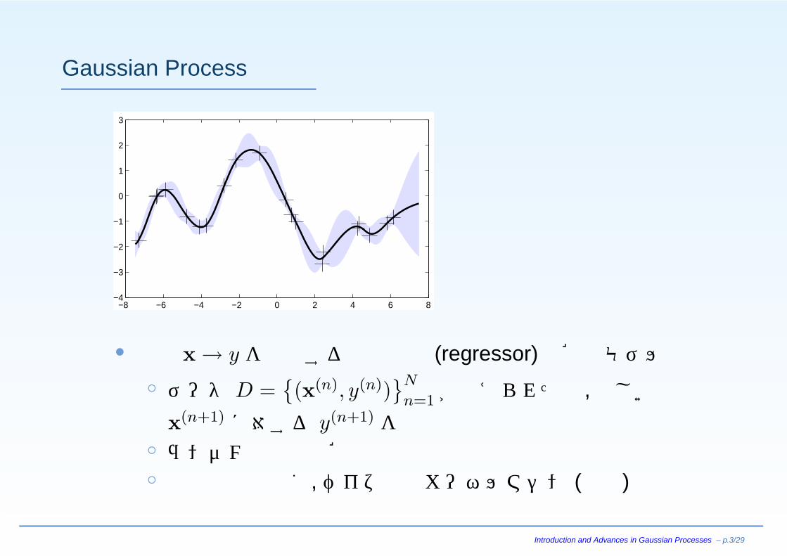
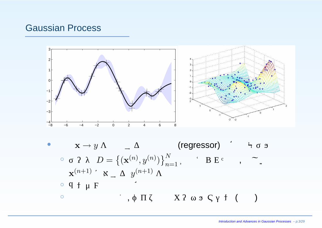
• 入力 x → y を予測する回帰関数 (regressor)の確率モデル

◦ データ D ={(x(n), y(n))

}N

n=1が与えられた時, 新しい

x(n+1) に対する y(n+1) を予測◦ ランダムな関数の確率分布◦ 連続空間で動く,ベイズ的なカーネルマシン (後で)



−8 −6 −4 −2 0 2 4 6 8−4

−3

−2

−1

0

1

2

3


◦ データ D ={(x(n), y(n))

}N





−8 −6 −4 −2 0 2 4 6 8−4

−3

−2

−1

0

1

2

3


◦ データ D ={(x(n), y(n))

}N




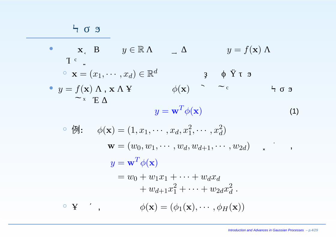
線形回帰モデル

• 入力 xから出力 y ∈ Rを予測する回帰関数 y = f(x)を求めたい◦ x = (x1, · · · , xd) ∈ R

d は時間や任意のベクトル• y = f(x)を, xを一般の関数 φ(x)で変換した上で線形モデルで表してみる

y = wT φ(x) (1)

◦ 例: φ(x) = (1, x1, · · · , xd, x21, · · · , x2

d)

w = (w0, w1, · · · , wd, wd+1, · · · , w2d) とおくと,

y = wT φ(x)

= w0 + w1x1 + · · · + wdxd

+ wd+1x21 + · · · + w2dx

2d .

◦ 一般に,基底関数 φ(x) = (φ1(x), · · · , φH(x))


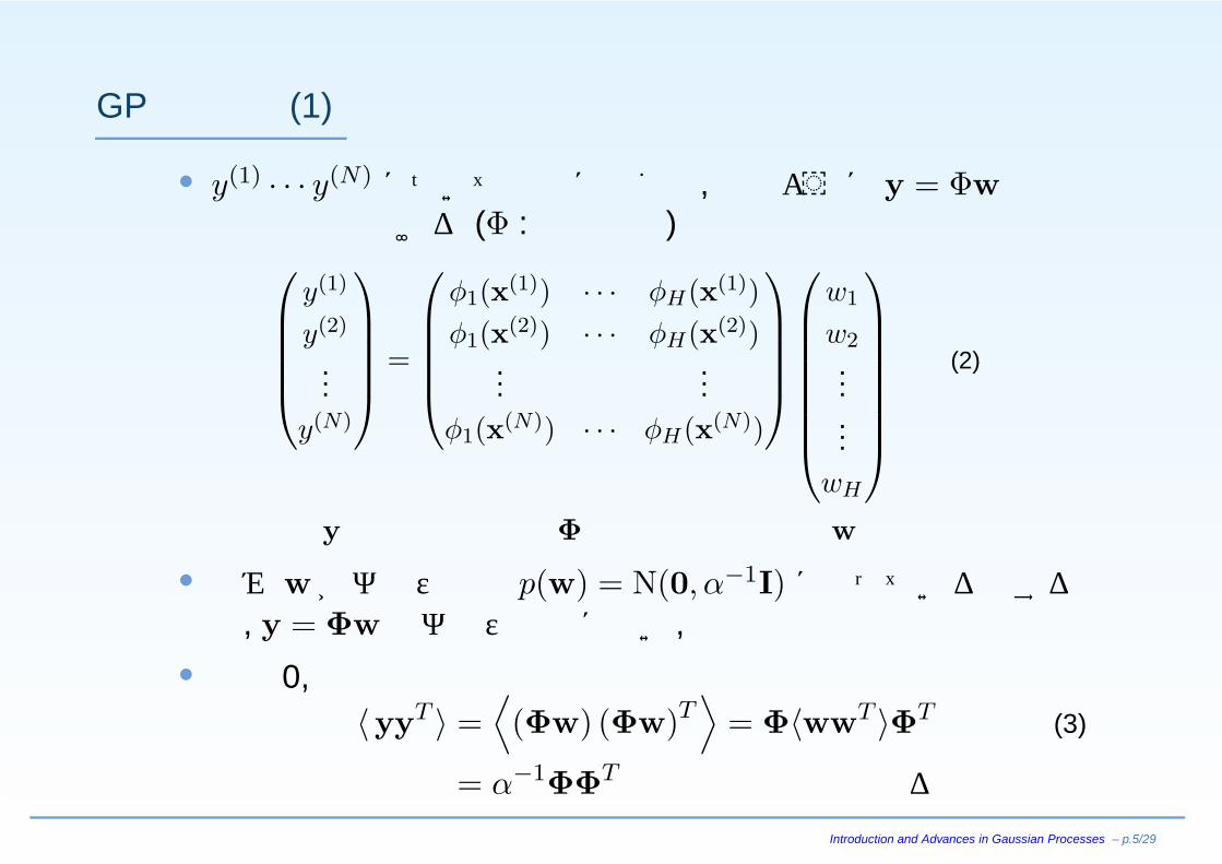
GPの導入 (1)

• y(1) · · · y(N) について同時に書くと, 下のように y = Φw と行列形式で書ける (Φ : 計画行列)⎛

⎜⎜⎜⎜⎝y(1)

y(2)

...y(N)

⎞⎟⎟⎟⎟⎠ =

⎛⎜⎜⎜⎜⎝

φ1(x(1)) · · · φH(x(1))φ1(x(2)) · · · φH(x(2))

......

φ1(x(N)) · · · φH(x(N))

⎞⎟⎟⎟⎟⎠

⎛⎜⎜⎜⎜⎜⎜⎜⎝

w1

w2

...

...wH

⎞⎟⎟⎟⎟⎟⎟⎟⎠

(2)

y Φ w

• 重み w がガウス分布 p(w) = N(0, α−1I)に従っているとすると, y = Φw もガウス分布に従い,

• 平均 0,分散〈yyT 〉 =

⟨(Φw) (Φw)T

⟩= Φ〈wwT 〉ΦT (3)

= α−1ΦΦT の正規分布となる


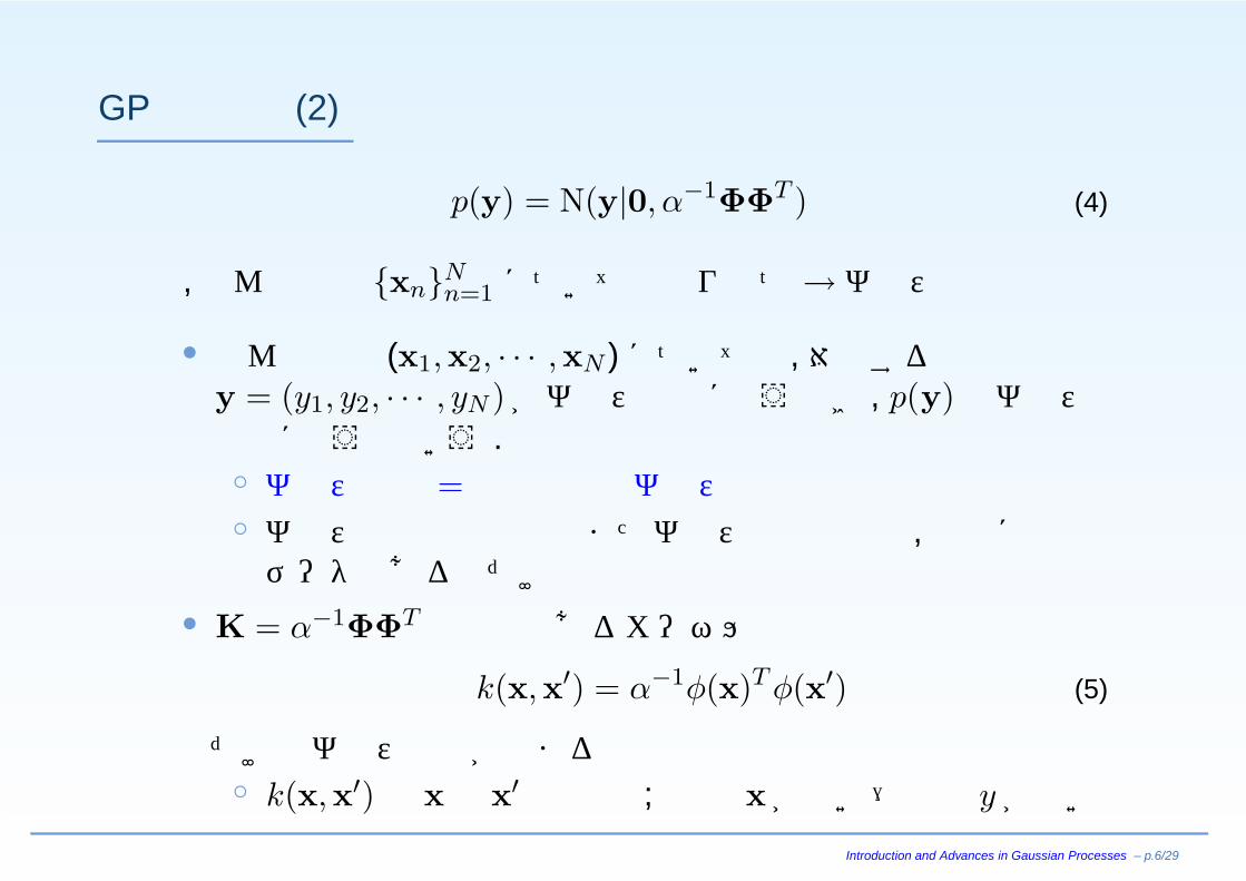
GPの導入 (2)

p(y) = N(y|0, α−1ΦΦT ) (4)

は,どんな入力 {xn}Nn=1 についても成り立つ→ガウス過程の定義

• どんな入力 (x1,x2, · · · ,xN )についても,対応する出力y = (y1, y2, · · · , yN )がガウス分布に従うとき, p(y)はガウス過程に従うという.◦ ガウス過程 =無限次元のガウス分布◦ ガウス分布の周辺化はまたガウス分布なので, 実際にはデータのある所だけの有限次元

• K = α−1ΦΦT の要素であるカーネル関数

k(x,x′) = α−1φ(x)T φ(x′) (5)

だけでガウス分布が定まる◦ k(x,x′)は xと x′の距離 ; 入力 xが近い→出力 y が近い


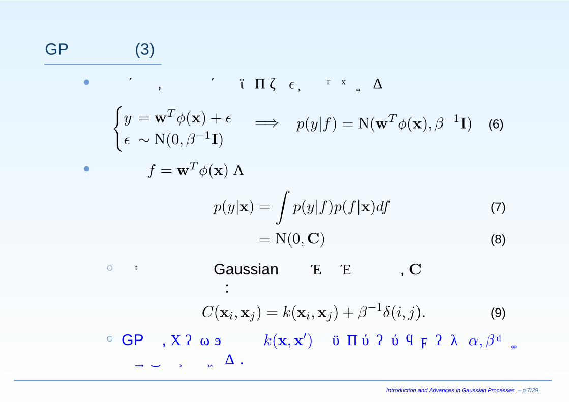
GPの導入 (3)

• 実際には,観測値にはノイズ εが乗っている{y = wT φ(x) + ε

ε ∼ N(0, β−1I)=⇒ p(y|f) = N(wT φ(x), β−1I) (6)

• 途中の f = wT φ(x)を積分消去

p(y|x) =∫

p(y|f)p(f |x)df (7)

= N(0,C) (8)

◦ 二つの独立なGaussianの畳み込みなので, Cの要素は共分散の単純な和:

C(xi,xj) = k(xi,xj) + β−1δ(i, j). (9)

◦ GPは,カーネル関数 k(x,x′)とハイパーパラメータ α, β だけで表すことができる.


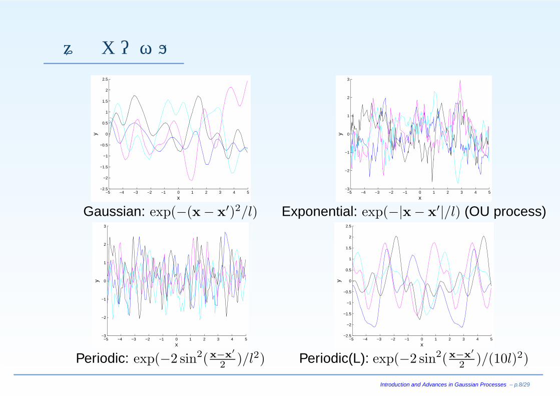
様々なカーネル

−5 −4 −3 −2 −1 0 1 2 3 4 5−2.5

−2

−1.5

−1

−0.5

0

0.5

1

1.5

2

2.5

x

y

−5 −4 −3 −2 −1 0 1 2 3 4 5−3

−2

−1

0

1

2

3

x

y

Gaussian: exp(−(x − x′)2/l) Exponential: exp(−|x − x′|/l) (OU process)

−5 −4 −3 −2 −1 0 1 2 3 4 5−3

−2

−1

0

1

2

3

x

y

−5 −4 −3 −2 −1 0 1 2 3 4 5−2.5

−2

−1.5

−1

−0.5

0

0.5

1

1.5

2

2.5

xy

Periodic: exp(−2 sin2(x−x′2 )/l2) Periodic(L): exp(−2 sin2(x−x′

2 )/(10l)2)


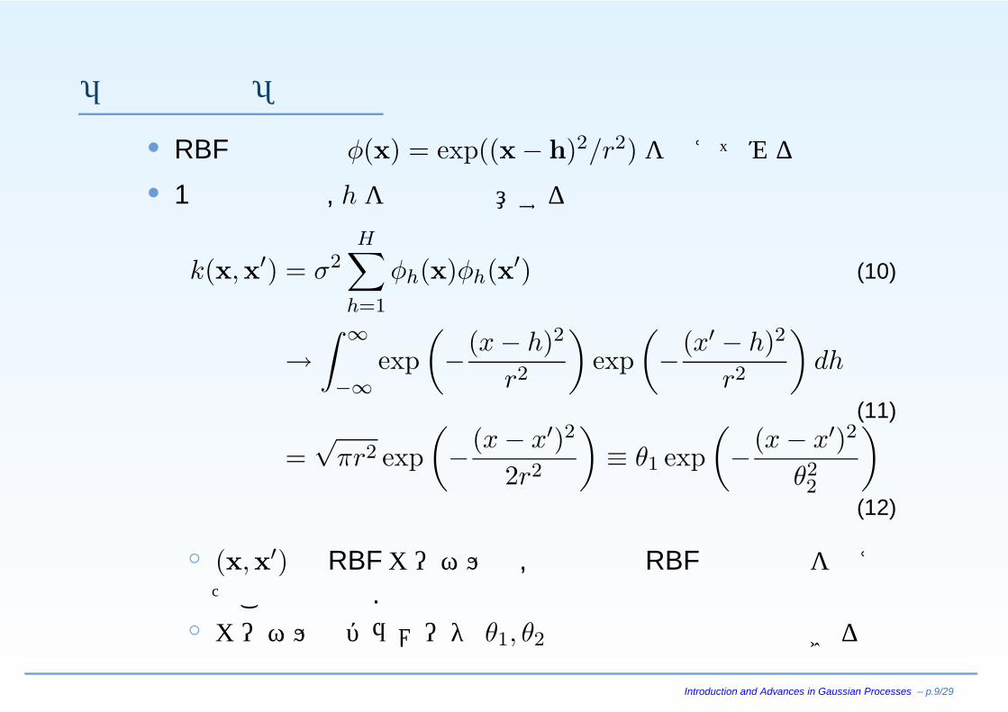
「基底関数」の消去

• RBF基底関数 φ(x) = exp((x − h)2/r2)を考えてみる• 1次元の場合, hを無限個用意すると

k(x,x′) = σ2H∑

h=1

φh(x)φh(x′) (10)

→∫ ∞

−∞exp

(−(x − h)2

r2

)exp

(−(x′ − h)2

r2

)dh

(11)

=√

πr2 exp(−(x − x′)2

2r2

)≡ θ1 exp

(−(x − x′)2

θ22

)(12)

◦ (x,x′)の RBFカーネルは,無限個の RBF基底関数を考えたことと等価.

◦ カーネルのパラメータ θ1, θ2 は最尤推定で最適化できる


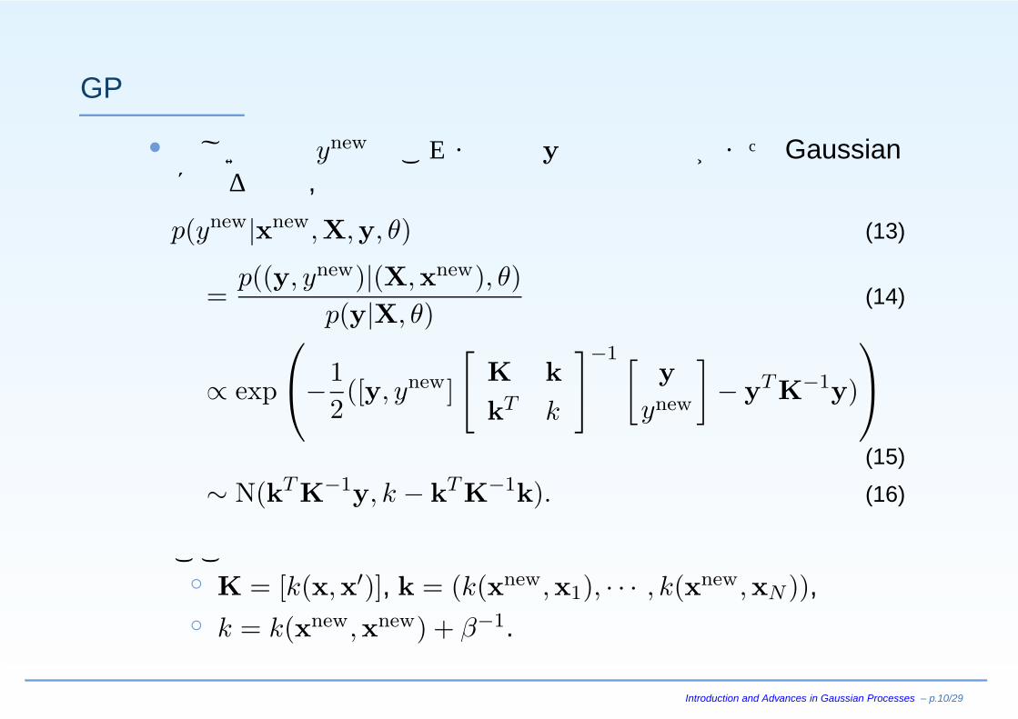
GPの予測

• 新しい入力 ynew とこれまでの y の結合分布がまたGaussianになるので,

p(ynew|xnew,X,y, θ) (13)

=p((y, ynew)|(X,xnew), θ)

p(y|X, θ)(14)

∝ exp

⎛⎝−1

2([y, ynew]

[K kkT k

]−1 [y

ynew

]− yT K−1y)

⎞⎠(15)

∼ N(kT K−1y, k − kT K−1k). (16)

ここで◦ K = [k(x,x′)], k = (k(xnew,x1), · · · , k(xnew,xN )),◦ k = k(xnew,xnew) + β−1.


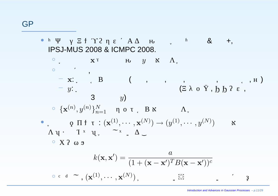
GPの適用例

• 『ガウシアンプロセスによる名演奏の学習』寺村&前田+,IPSJ-MUS 2008 & ICMPC 2008.◦ 楽譜情報 x→実際の演奏 y の対応を学習◦ 実際には,− x: 楽譜からの素性 (拍子,音高,音長,強弱指定,主旋律か,…)− y: 楽譜の指定と実際の出力との差 (アタック,リリース,強弱の 3種類の y)

◦ {x(n), y(n)}Nn=1 のセットから対応関係を学習

• 学習のポイント: (x(1), · · · ,x(N)) → (y(1), · · · , y(N))への対応を「まとめて」学習していること◦ カーネルは

k(x,x′) =a

(1 + (x − x′)T B(x − x′))c

◦ ただし, (x(1), · · · ,x(N))が時系列という仮定は無いのに注意


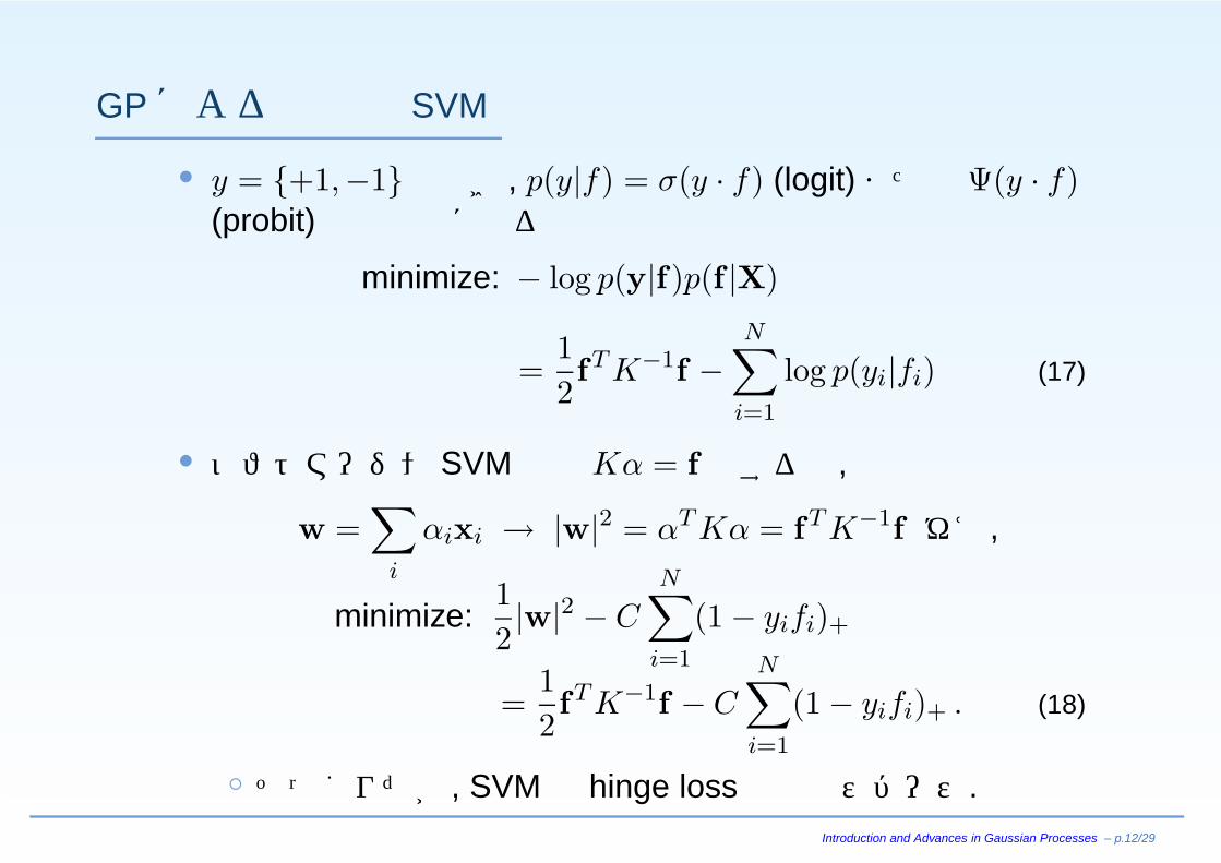
GPによる分類とSVM

• y = {+1,−1}のとき, p(y|f) = σ(y · f) (logit)またはΨ(y · f)(probit)で分類器になる

minimize: − log p(y|f)p(f |X)

=12fT K−1f −

N∑i=1

log p(yi|fi) (17)

• ソフトマージン SVMでは Kα = f とすると,

w =∑

i

αixi → |w|2 = αT Kα = fT K−1f ゆえ,

minimize:12|w|2 − C

N∑i=1

(1 − yifi)+

=12fT K−1f − C

N∑i=1

(1 − yifi)+ . (18)

◦ そっくりだが, SVMは hinge lossなのでスパース.Introduction and Advances in Gaussian Processes – p.12/29

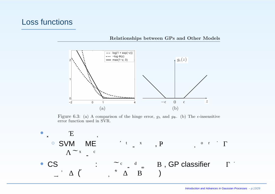
Loss functions

Relationships between GPs and Other Models

−2 0 1 4

0

1

2

log(1 + exp(−z))

−log Φ(z)

max(1−z, 0)

z

gε(z)

−ε 0 −ε.

(a) (b)

Figure 6.3: (a) A comparison of the hinge error, gλ and gΦ. (b) The ε-insensitiveerror function used in SVR.

• お馴染みの議論かも◦ SVMとMEの関係についても,以前工藤君がそっくりの議論をしていた

• CS研での議論: 分類したいだけなら, GP classifierは回りくどすぎる (他の理由があるなら有効)


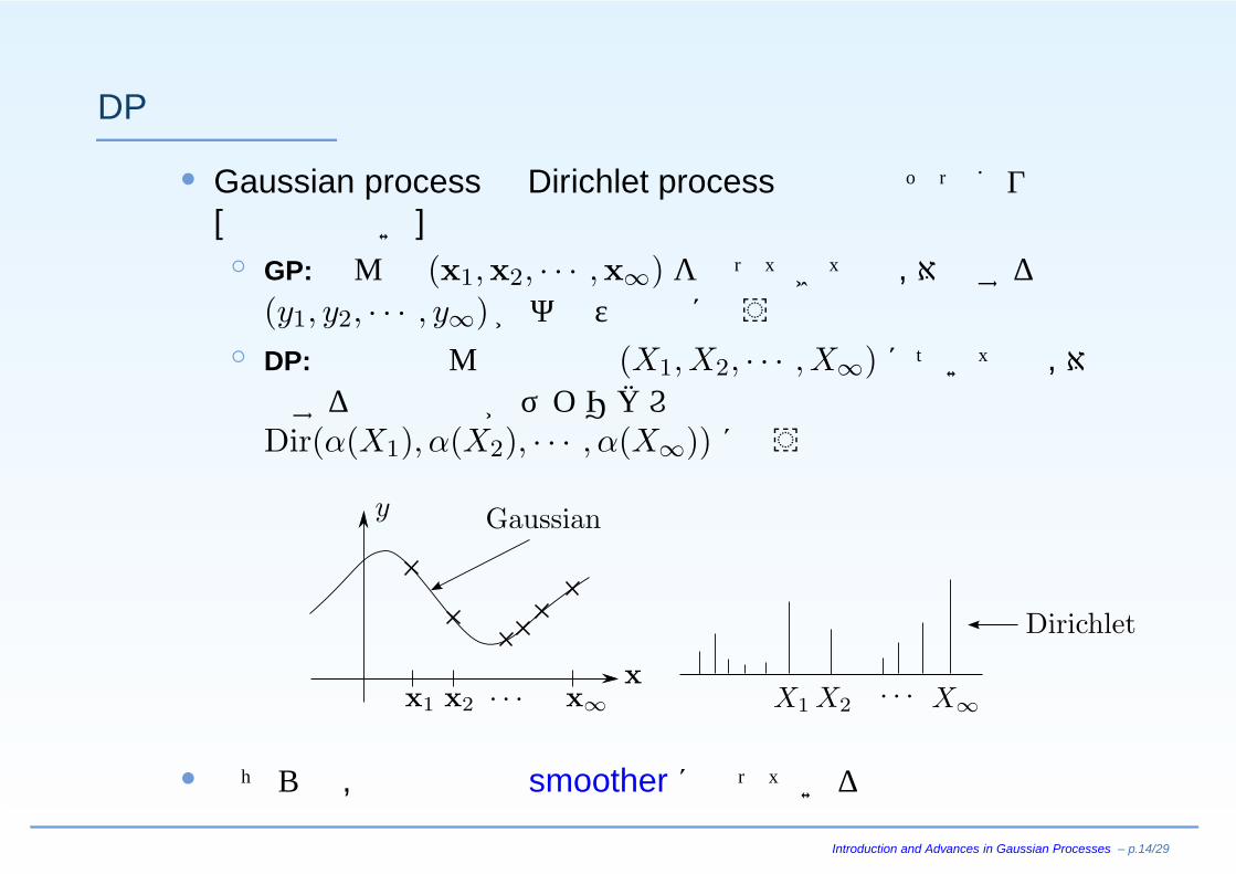
DPとの関係

• Gaussian processと Dirichlet processの定義はそっくり[偶然ではない]◦ GP:どんな (x1,x2, · · · ,x∞)をとってきても,対応する

(y1, y2, · · · , y∞)がガウス分布に従う◦ DP:空間のどんな離散化 (X1,X2, · · · ,X∞)についても,対応する離散分布がディリクレ分布Dir(α(X1), α(X2), · · · , α(X∞))に従う

• どちらも,無限次元の smootherになっている


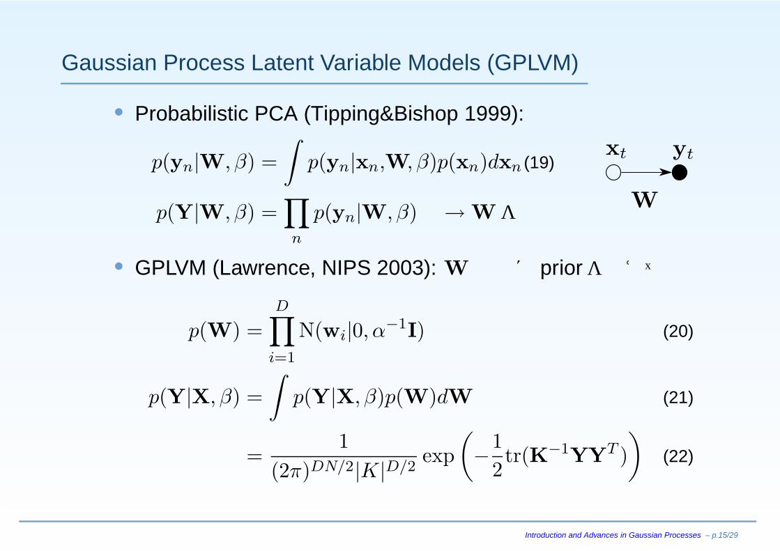
Gaussian Process Latent Variable Models (GPLVM)

• Probabilistic PCA (Tipping&Bishop 1999):

p(yn|W, β) =∫

p(yn|xn,W, β)p(xn)dxn (19)

p(Y|W, β) =∏n

p(yn|W, β) → Wを最適化

• GPLVM (Lawrence, NIPS 2003): Wの方に priorを与えて積分消去

p(W) =D∏

i=1

N(wi|0, α−1I) (20)

p(Y|X, β) =∫

p(Y|X, β)p(W)dW (21)

=1

(2π)DN/2|K|D/2exp

(−1

2tr(K−1YYT )

)(22)


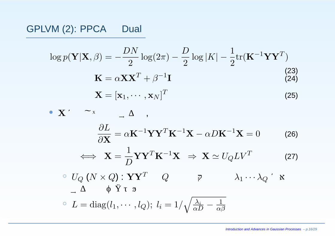
GPLVM (2): PPCAのDual

log p(Y|X, β) = −DN

2log(2π) − D

2log |K| − 1

2tr(K−1YYT )

(23)K = αXXT + β−1I (24)

X = [x1, · · · ,xN ]T (25)

• Xに関して微分すると,

∂L

∂X= αK−1YYT K−1X − αDK−1X = 0 (26)

⇐⇒ X =1D

YYT K−1X ⇒ X UQLV T (27)

◦ UQ (N × Q) : YYT の Q個の最大固有値 λ1 · · ·λQ に対応する固有ベクトル

◦ L = diag(l1, · · · , lQ); li = 1/√

λi

αD − 1αβ


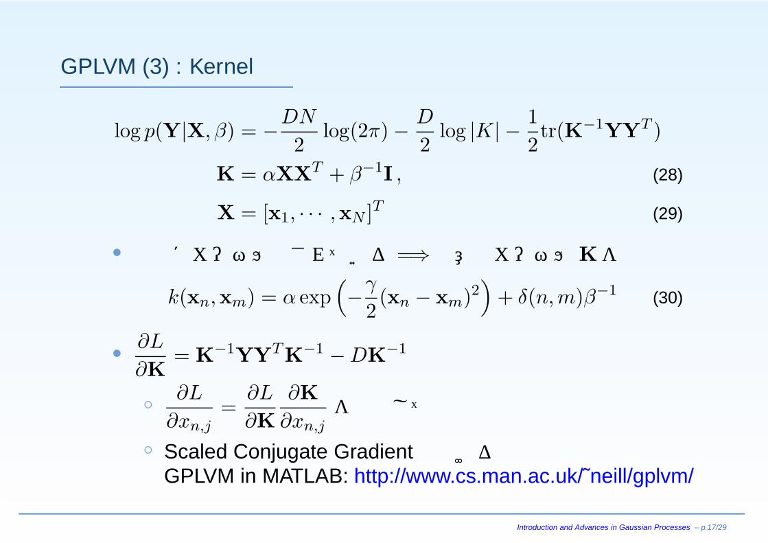
GPLVM (3) : Kernel化

log p(Y|X, β) = −DN

2log(2π) − D

2log |K| − 1

2tr(K−1YYT )

K = αXXT + β−1I , (28)

X = [x1, · · · ,xN ]T (29)

• 自然にカーネル化されている =⇒任意のカーネルKを導入

k(xn,xm) = α exp(−γ

2(xn − xm)2

)+ δ(n,m)β−1 (30)

• ∂L

∂K= K−1YYTK−1 − DK−1

◦ ∂L

∂xn,j=

∂L

∂K∂K

∂xn,jを適用して微分

◦ Scaled Conjugate Gradientで解けるGPLVM in MATLAB: http://www.cs.man.ac.uk/˜neill/gplvm/


http://www.cs.man.ac.uk/~neill/gplvm/

GPLVM (4):例

−0.8 −0.6 −0.4 −0.2 0 0.2 0.4 0.6−0.5

−0.4

−0.3

−0.2

−0.1

0

0.1

0.2

0.3

−0.2 −0.1 0 0.1 0.2 0.3

−0.25

−0.2

−0.15

−0.1

−0.05

0

0.05

0.1

0.15

0.2

0.4

0.6

0.8

1

1.2

1.4

1.6

1.8

2

2.2

2.4

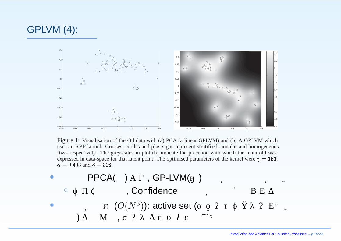
Figure 1: Visualisation of the Oil data with (a) PCA (a linear GPLVM) and (b) A GPLVM whichuses an RBF kernel. Crosses, circles and plus signs represent stratified, annular and homogeneousflows respectively. The greyscales in plot (b) indicate the precision with which the manifold wasexpressed in data-space for that latent point. The optimised parameters of the kernel were �� , �� and �� .

• 線形の PPCA(左)より, GP-LVM(右)の方が分離性能が高い◦ ベイズなので, Confidenceの分布が同時に得られる

• 計算量が問題 (O(N3)): active set (サポートベクターみたいなもの)を選んで,データをスパース化して最適化


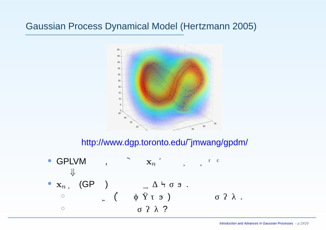
Gaussian Process Dynamical Model (Hertzmann 2005)

http://www.dgp.toronto.edu/˜jmwang/gpdm/

• GPLVMでは,潜在変数 xn に分布がなかった⇓

• xn が (GPで)時間発展するモデル.◦ 人間の動き (角度ベクトル)等の時系列データ.◦ 自然言語の時系列データ?


http://www.dgp.toronto.edu/~jmwang/gpdm/

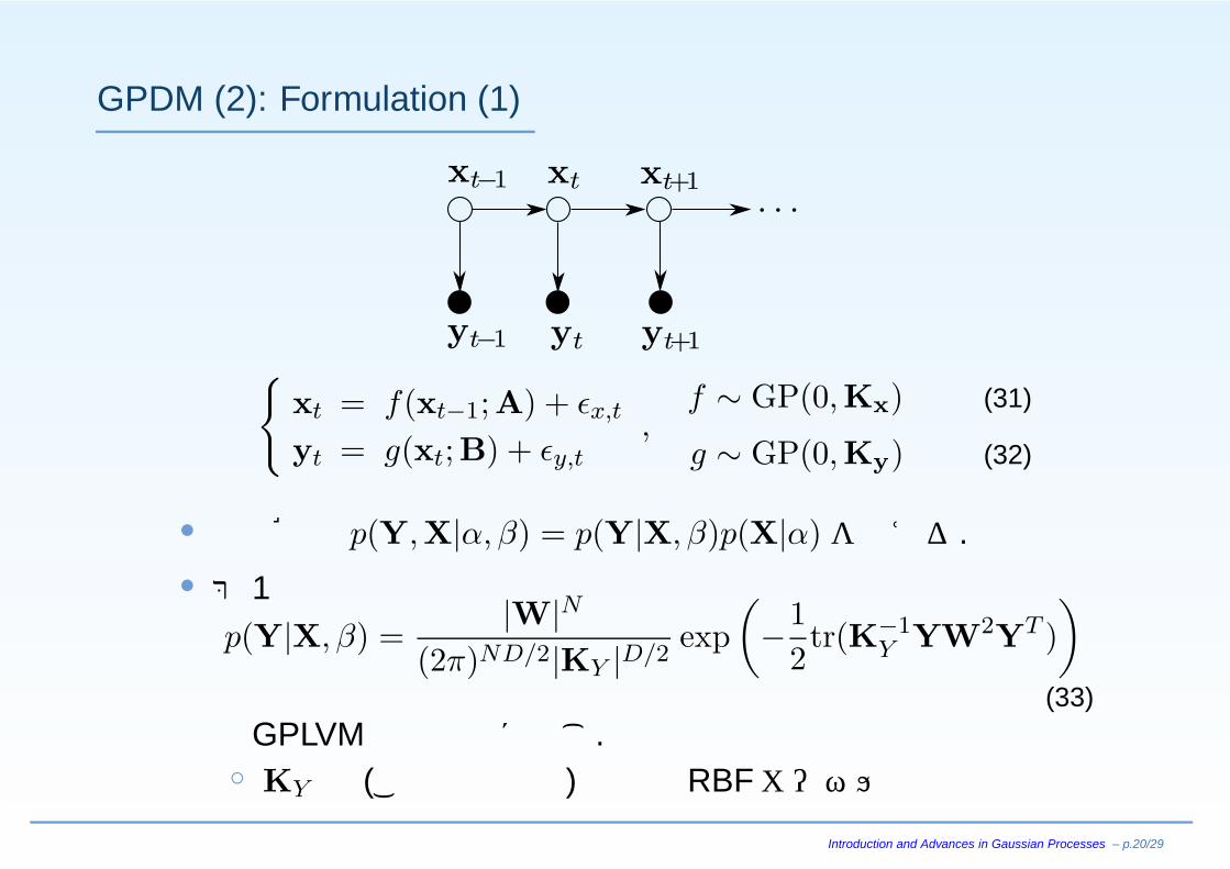
GPDM (2): Formulation (1)

{xt = f(xt−1;A) + εx,t

yt = g(xt;B) + εy,t,

f ∼ GP(0,Kx) (31)

g ∼ GP(0,Ky) (32)

• 結合確率 p(Y,X|α, β) = p(Y|X, β)p(X|α)を考える.

• 第 1項p(Y|X, β) =

|W|N(2π)ND/2|KY |D/2

exp(−1

2tr(K−1

Y YW2YT ))

(33)はGPLVMと基本的に同じ.◦ KY は (この論文では)普通の RBFカーネル


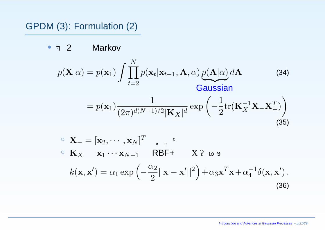
GPDM (3): Formulation (2)

• 第 2項はMarkov時系列

p(X|α) = p(x1)∫ N∏

t=2

p(xt|xt−1,A, α) p(A|α)︸︷︷︸Gaussian

dA (34)

= p(x1)1

(2π)d(N−1)/2|KX |d exp(−1

2tr(K−1

X X−XT−)

)(35)

◦ X− = [x2, · · · ,xN ]T とおいた◦ KX は x1 · · ·xN−1 の RBF+線形カーネル

k(x,x′) = α1 exp(−α2

2||x − x′||2

)+α3xT x+α−1

4 δ(x,x′) .

(36)


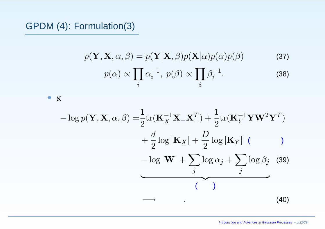
GPDM (4): Formulation(3)

p(Y,X, α, β) = p(Y|X, β)p(X|α)p(α)p(β) (37)

p(α) ∝∏

i

α−1i , p(β) ∝

∏i

β−1i . (38)

• 対数尤度は

− log p(Y,X, α, β) =12tr(K−1

X X−XT−) +

12tr(K−1

Y YW2YT )

+d

2log |KX | + D

2log |KY | (正則化項)

− log |W| +∑

j

log αj +∑

j

log βj

︸︷︷︸(定数)

(39)

−→最小化. (40)


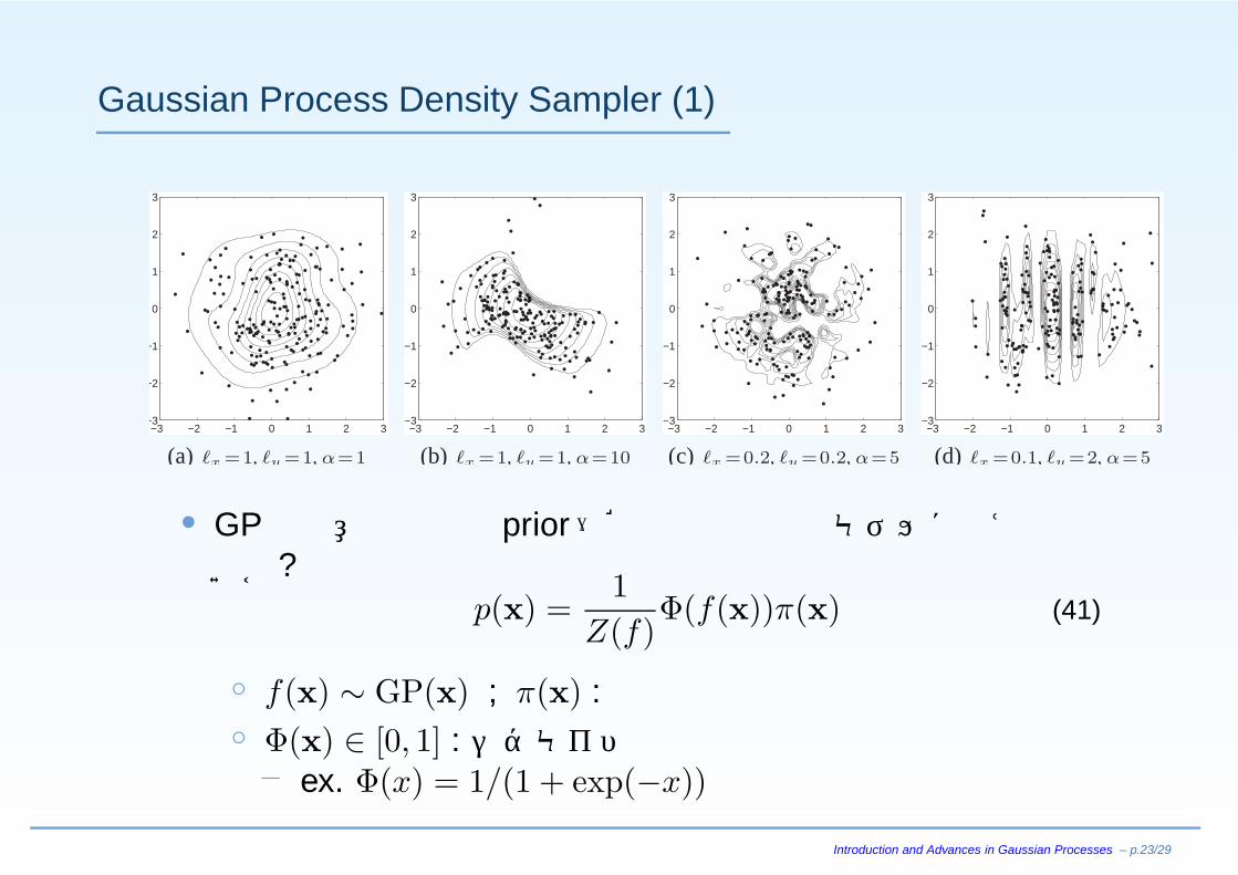
Gaussian Process Density Sampler (1)

−3 −2 −1 0 1 2 3−3

−2

−1

0

1

2

3

(a) �x =1, �y =1, α=1

−3 −2 −1 0 1 2 3−3

−2

−1

0

1

2

3

(b) �x =1, �y =1, α=10

−3 −2 −1 0 1 2 3−3

−2

−1

0

1

2

3

(c) �x =0.2, �y =0.2, α=5

−3 −2 −1 0 1 2 3−3

−2

−1

0

1

2

3

(d) �x =0.1, �y =2, α=5

• GPは任意の関数の prior→確率密度関数のモデルに使えないか?

p(x) =1

Z(f)Φ(f(x))π(x) (41)

◦ f(x) ∼ GP(x) ; π(x) : 事前分布◦ Φ(x) ∈ [0, 1] : シグモイド関数− ex. Φ(x) = 1/(1 + exp(−x))


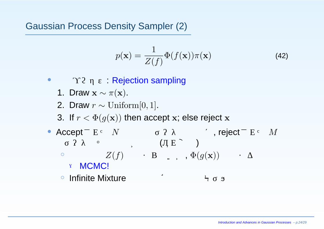
Gaussian Process Density Sampler (2)

p(x) =1

Z(f)Φ(f(x))π(x) (42)

• 生成プロセス: Rejection sampling1. Draw x ∼ π(x).2. Draw r ∼ Uniform[0, 1].3. If r < Φ(g(x)) then accept x; else reject x

• AcceptされたN 個の観測データの背後に, rejectされたM 個のデータとその場所が存在 (隠れ変数)◦ 分配関数 Z(f)は求まらないが, Φ(g(x))は求まる→MCMC!

◦ Infinite Mixtureとは別の確率密度のモデル化


Gaussian Processes for NLP?

• 言語では出力 y = (y1, · · · , yN )はGaussianではないので,直接は使えない

• 隠れ変数の (連続的な)分布に使える可能性は高い◦ Ex: Latent CCA in (Haghighi+, ACL 2008)

• 分類もできるが,特にGPでないといけない理由は希少• 言語+αのモデル化に特に重要だと思われる


まとめ

• Gaussian Process…連続的な関数のベイズモデル◦ カーネル関数で定義される, 無限次元のガウス分布◦ 基底関数の空間での線形モデルで, 重みを積分消去したもの

• カーネル設計が重要◦ カーネルの違いにより, さまざまな振舞い◦ カーネルのパラメータは, 確率モデルなので最適化できる

• 回帰問題だけでなく, 隠れ変数や確率分布のモデルにも使える,確率モデルの Building Block

• 計算量が課題→研究は最近様々に進んでいる


Literature

• “Gaussian Process Dynamical Models”. J. Wang, D. Fleet,and A. Hertzmann. NIPS 2005.http://www.dgp.toronto.edu/ jmwang/gpdm/

• “Gaussian Process Latent Variable Models for Visualizationof High Dimensional Data”. Neil D. Lawrence, NIPS 2003.

• “The Gaussian Process Density Sampler”. Ryan PrescottAdams, Iain Murray and David MacKay. NIPS 2008.

• “Archipelago: Nonparametric Bayesian Semi-SupervisedLearning”. Ryan Prescott Adams and Zoubin Ghahramani.ICML 2009.



Readings

• “Gaussian Processes for Machine Learning”. Rasmussenand Williams, MIT Press, 2006.http://www.gaussianprocess.org/gpml/

• “Gaussian Processes — A Replacement for SupervisedNeural Networks?”. David MacKay, Lecture notes at NIPS1997. http://www.inference.phy.cam.ac.uk/mackay/GP/◦ Videolectures.net: “Gaussian Process Basics.”

http://videolectures.net/gpip06_mackay_gpb/• Pattern Recognition and Machine Learning, Chapter 6.

Christopher Bishop, Springer, 2006.http://ibisforest.org/index.php?PRML

• ガウス過程に関するメモ (1). 正田備也, 2007.http://www.iris.dti.ne.jp/˜tmasada/2007071101.pdf


http://www.gaussianprocess.org/gpml/

http://www.inference.phy.cam.ac.uk/mackay/GP/

http://videolectures.net/gpip06_mackay_gpb/

http://ibisforest.org/index.php?PRML

http://www.iris.dti.ne.jp/~tmasada/2007071101.pdf

Codes

• GPML MATLAB codes.http://www.gaussianprocess.org/gpml/code/

• GPLVM MATLAB/C++ codes.http://www.cs.manchester.ac.uk/˜neill/gplvm/

• GPDM code. http://www.dgp.toronto.edu/˜jmwang/gpdm/


http://www.gaussianprocess.org/gpml/code/

http://www.cs.manchester.ac.uk/~neill/gplvm/


Documents

Introduction and Advances in Gaussian Processeschasen.org/~daiti-m/paper/svm2009advgp.pdfH(x)) Introduction and Advances in Gaussian Processes – p.4/29 GP の導入(1) • y(1) ···y(N)