Introduction to Descriptive Statistics - MIT

Introduction to Descriptive Statistics17.871

Spring 2012

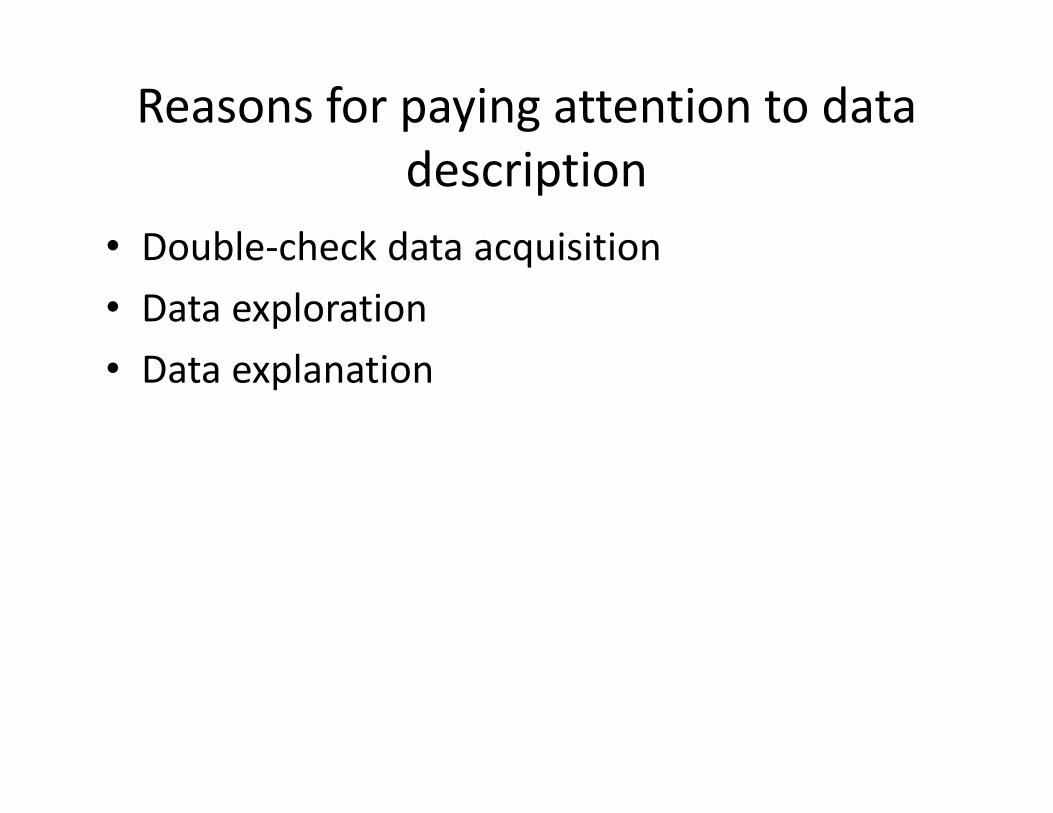
Reasons for paying attention to data description

• Double‐check data acquisition• Data exploration• Data explanation

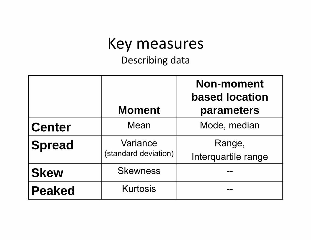
Key measuresDescribing data

Moment

Non-moment based location

parametersCenter Mean Mode, median

Spread Variance (standard deviation)

Range,Interquartile range

Skew Skewness --

Peaked Kurtosis --

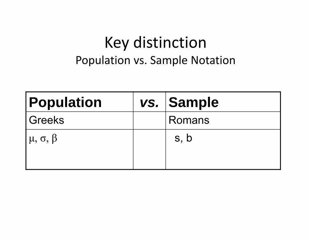
Key distinctionPopulation vs. Sample Notation

Population vs. SampleGreeks Romansμ, σ, β s, b

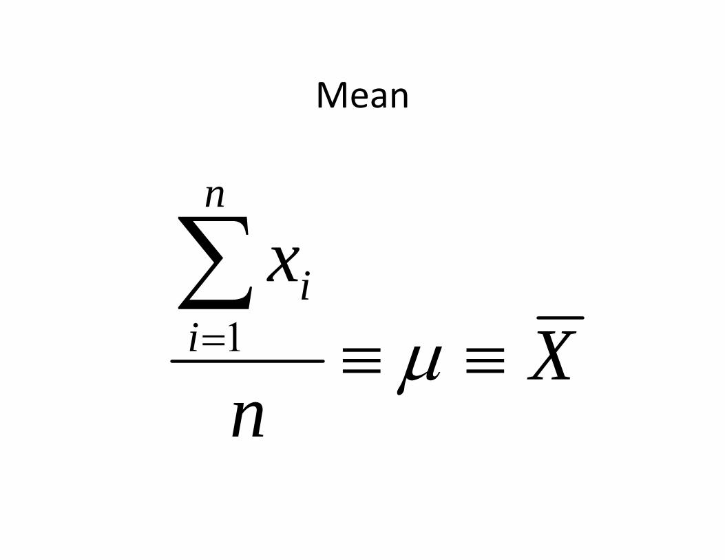
Mean

Xn

xn

ii

1

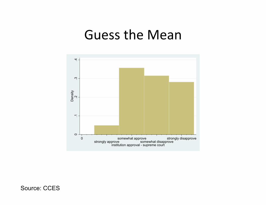
Guess the Mean

Source: CCES

0.1

.2.3

.4D

ensi

ty

0strongly approve

somewhat approvesomewhat disapprove

strongly disapprove

institution approval - supreme court

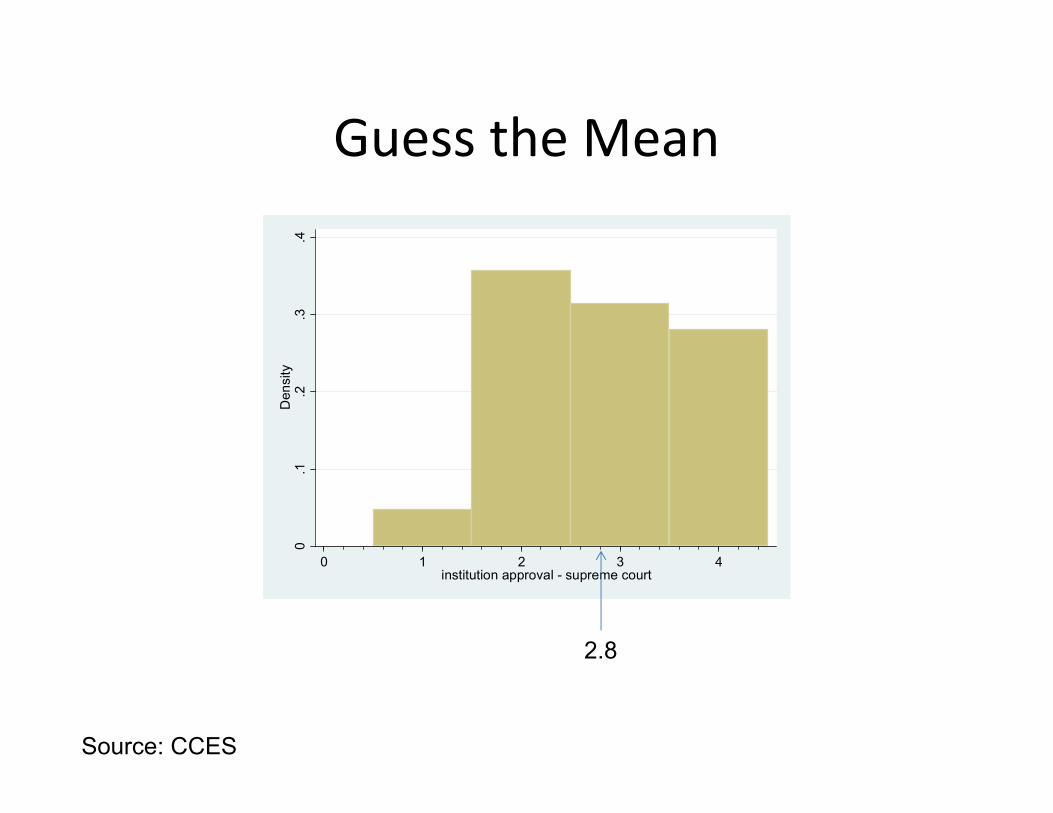
Guess the Mean

Source: CCES

0.1

.2.3

.4D

ensi

ty

0 1 2 3 4institution approval - supreme court

Guess the Mean

Source: CCES

0.1

.2.3

.4D

ensi

ty


2.8

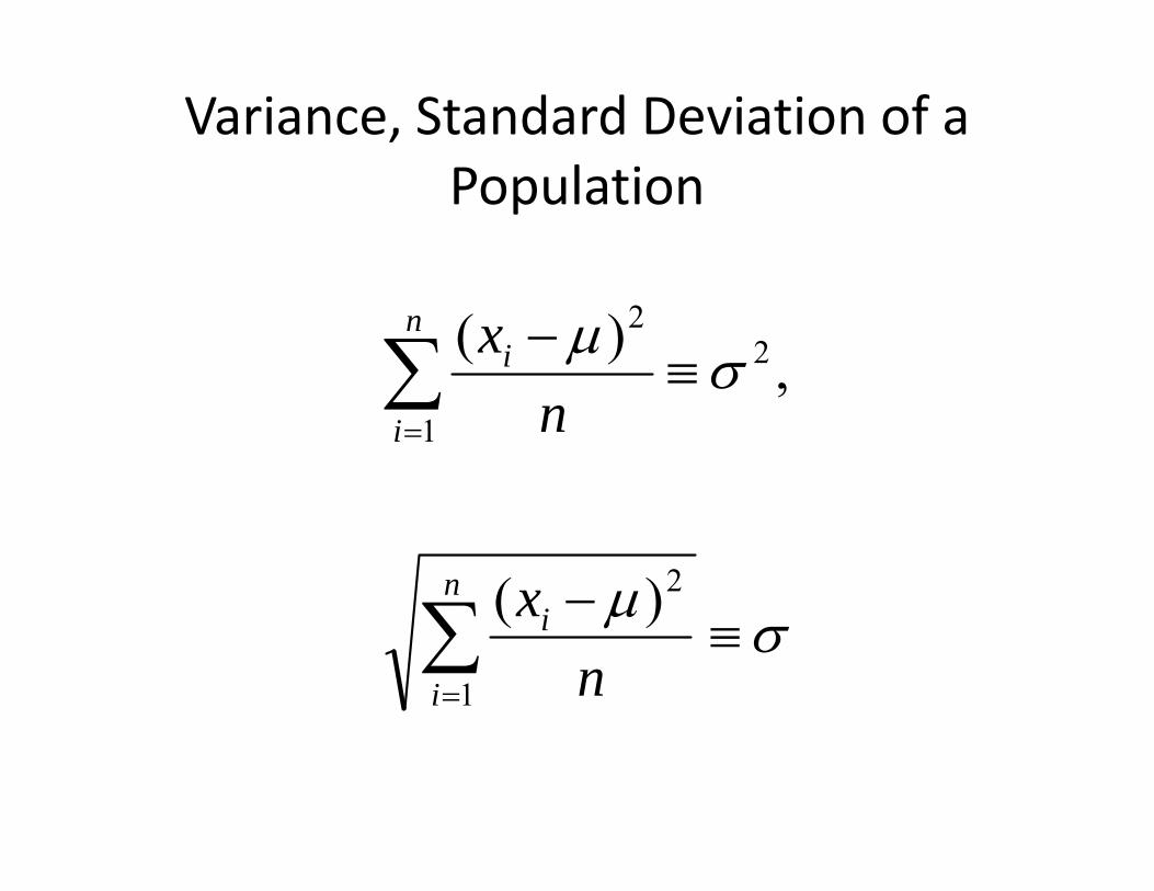
Variance, Standard Deviation of a Population

n

i

i

n

i

i

nx

nx

1

2

2

1

2

)(

,)(

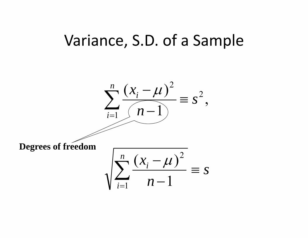
Variance, S.D. of a Sample

sn

x

sn

x

n

i

i

n

i

i

1

2

2

1

2

1)(

,1

)(

Degrees of freedom

Guess

What was the mean and standard deviation of the MIT undergraduatepopulation on Registration Day, Fall 2012?

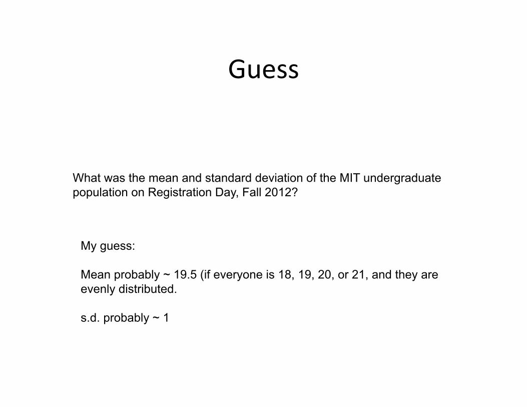
Guess

What was the mean and standard deviation of the MIT undergraduatepopulation on Registration Day, Fall 2012?

My guess:

Mean probably ~ 19.5 (if everyone is 18, 19, 20, or 21, and they are evenly distributed.

s.d. probably ~ 1

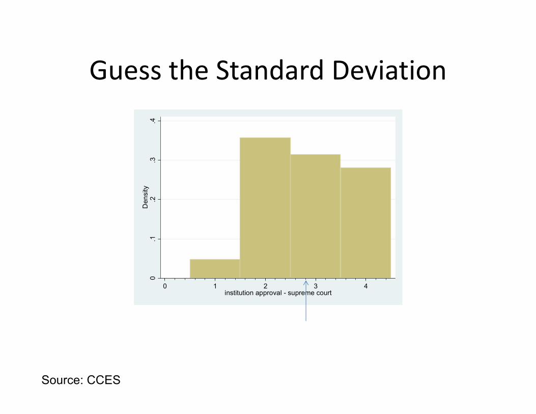
Guess the Standard Deviation

Source: CCES

0.1

.2.3

.4D

ensi

ty


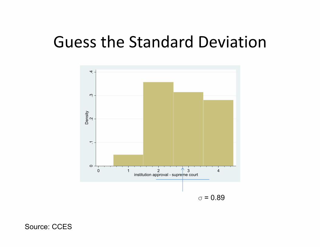
Guess the Standard Deviation

Source: CCES

0.1

.2.3

.4D

ensi

ty


F = 0.89

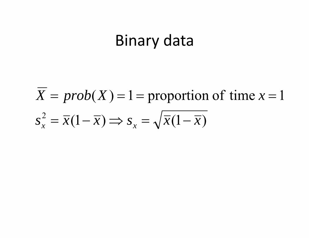
Binary data

)1()1(

1 timeof proportion1)(2 xxsxxs

xXprobX

xx

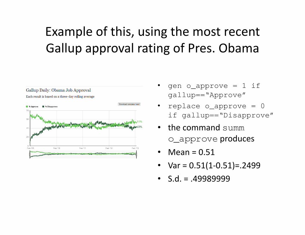
Example of this, using the most recent Gallup approval rating of Pres. Obama

• gen o_approve = 1 if gallup==“Approve”

• replace o_approve = 0 if gallup==“Disapprove”

• the command summo_approve produces

• Mean = 0.51• Var = 0.51(1‐0.51)=.2499• S.d. = .49989999

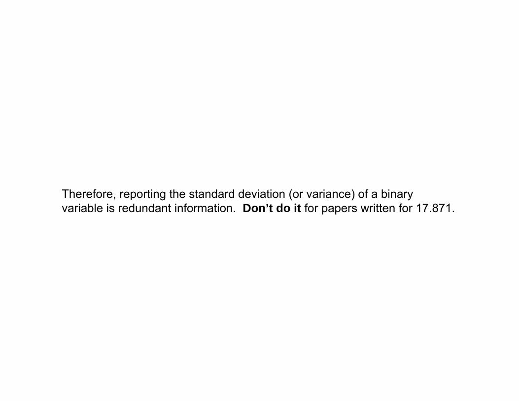
Therefore, reporting the standard deviation (or variance) of a binary variable is redundant information. Don’t do it for papers written for 17.871.

Non‐moment base measures of center or spread

• Central tendency– Mode– Median

• Spread– Range– Interquartile range

Mode

• The most common value

Guess the Mode

Source: CCES

0.1

.2.3

.4D

ensi

ty


2.8

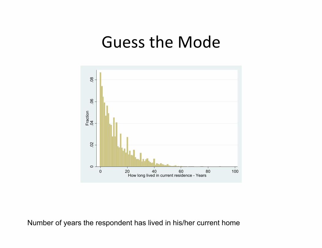
Guess the Mode

Number of years the respondent has lived in his/her current home

0.0

2.0

4.0

6.0

8Fr

actio

n

0 20 40 60 80 100How long lived in current residence - Years

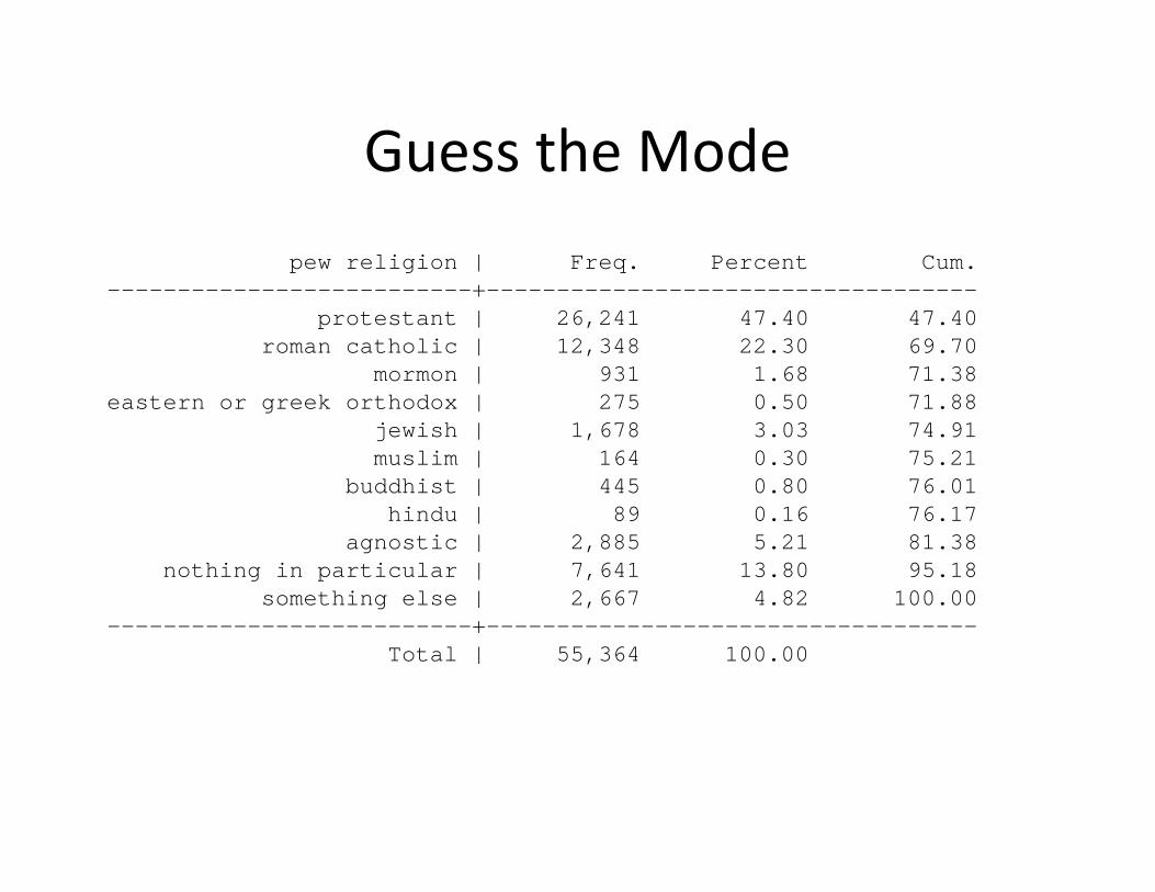
Guess the Modepew religion | Freq. Percent Cum.

--------------------------+-----------------------------------protestant | 26,241 47.40 47.40

roman catholic | 12,348 22.30 69.70mormon | 931 1.68 71.38

eastern or greek orthodox | 275 0.50 71.88jewish | 1,678 3.03 74.91muslim | 164 0.30 75.21

buddhist | 445 0.80 76.01hindu | 89 0.16 76.17

agnostic | 2,885 5.21 81.38nothing in particular | 7,641 13.80 95.18

something else | 2,667 4.82 100.00--------------------------+-----------------------------------

Total | 55,364 100.00

The mode is rarely an informative statistic about the central tendency of the data. It’s most useful in describing the “typical” observation of a categorical variable

Median

• The numerical value separating the upper half of a distribution from the lower half of the distribution– If N is odd, there is a unique median– If N is event, there is no unique median ‐‐‐ the convention is to average the two middle values

Guess the Median

Source: CCES

0.1

.2.3

.4D

ensi

ty


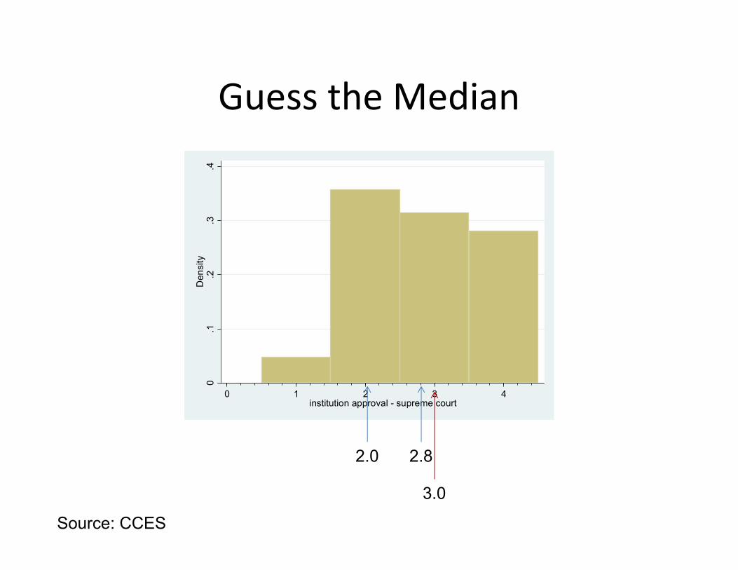
2.82.0

Guess the Median

Source: CCES

0.1

.2.3

.4D

ensi

ty


2.82.0

3.0

Guess the Median


0.0

2.0

4.0

6.0

8Fr

actio

n


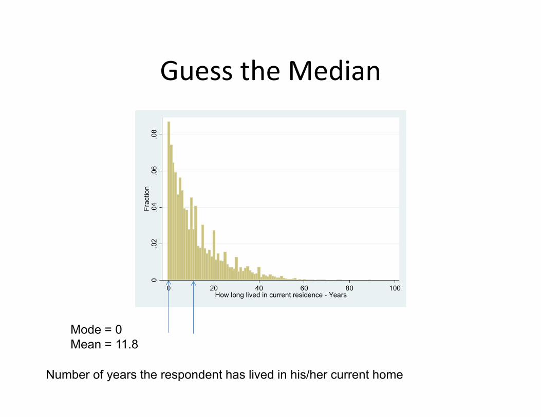
Mode = 0Mean = 11.8

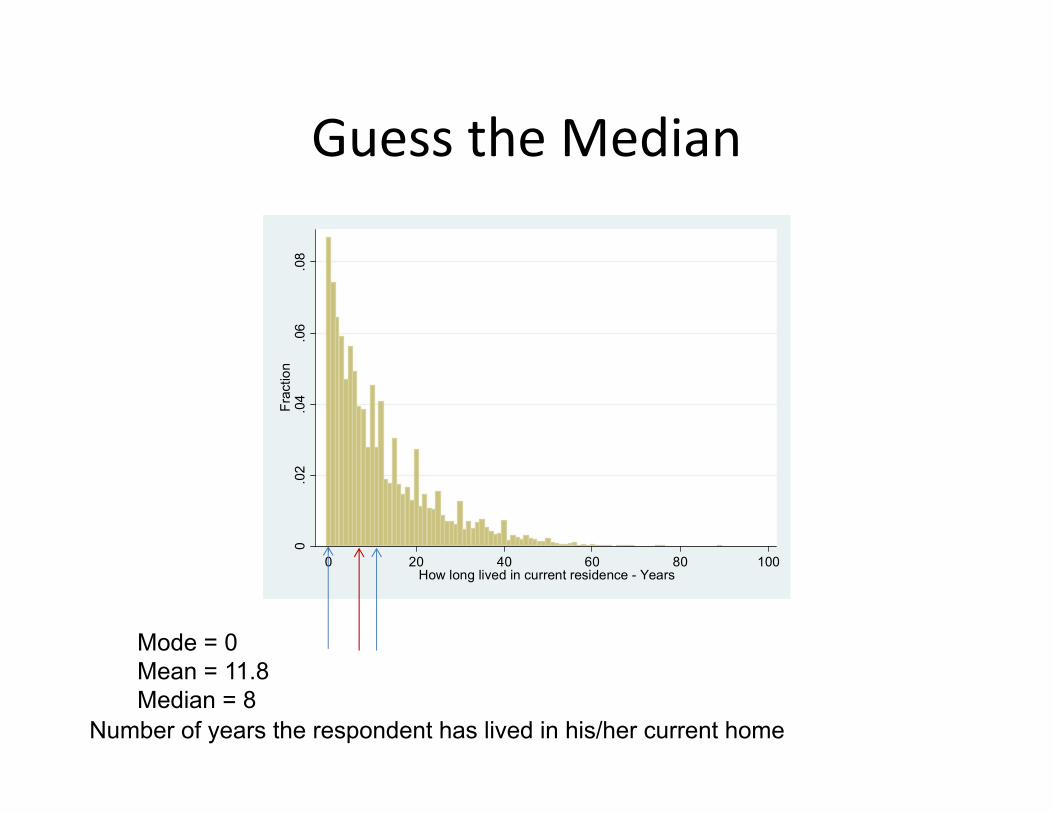
Guess the Median


0.0

2.0

4.0

6.0

8Fr

actio

n


Mode = 0Mean = 11.8Median = 8

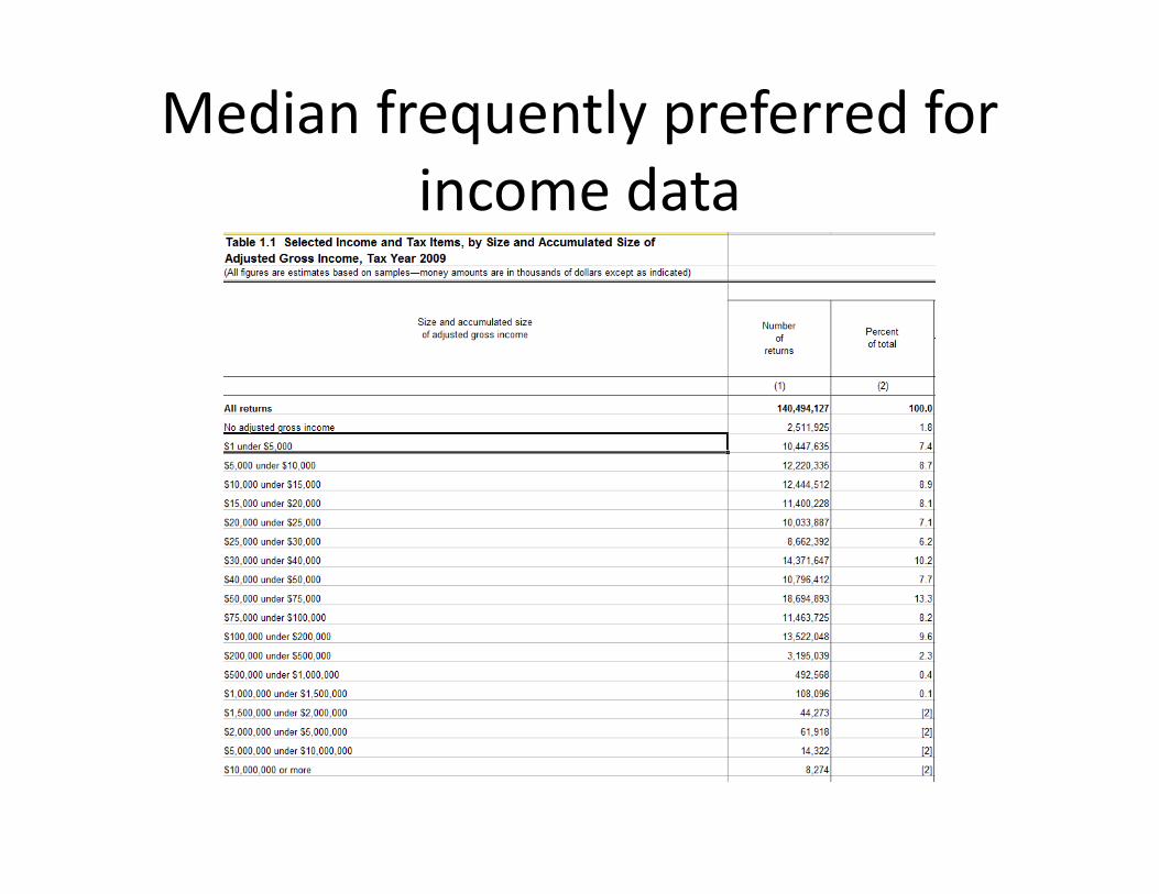
Median frequently preferred for income data

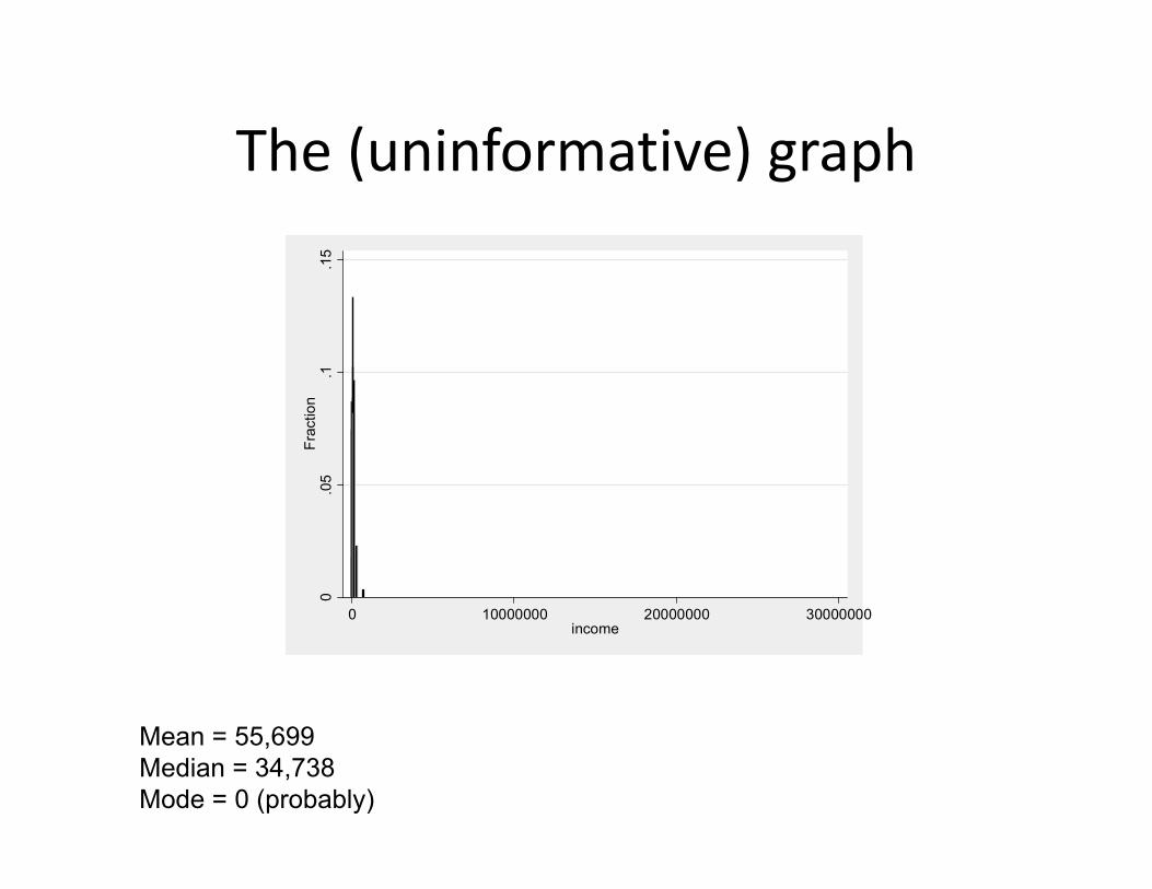
The (uninformative) graph

0.0

5.1

.15

Frac

tion

0 10000000 20000000 30000000income

Mean = 55,699Median = 34,738Mode = 0 (probably)

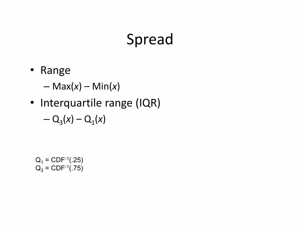
Spread

• Range– Max(x) – Min(x)

• Interquartile range (IQR)– Q3(x) – Q1(x)

Q1 = CDF-1(.25)Q3 = CDF-1(.75)

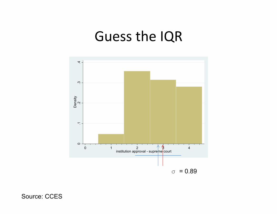
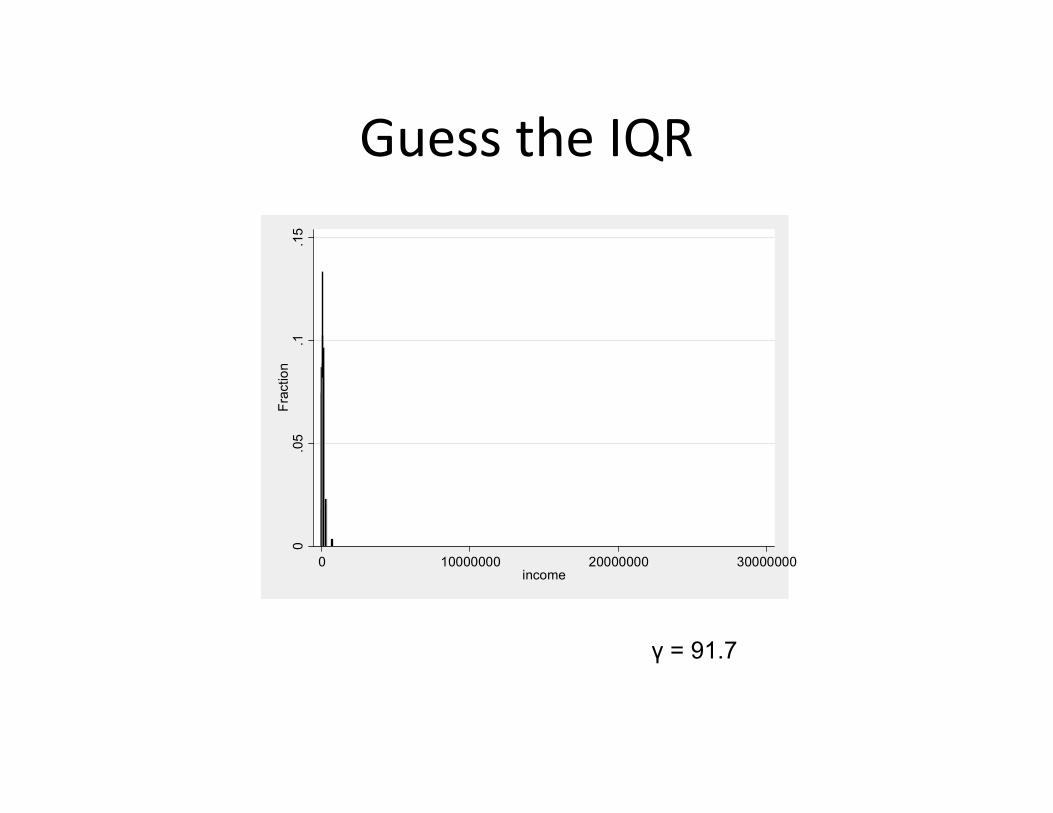
Guess the IQR

Source: CCES

0.1

.2.3

.4D

ensi

ty


F = 0.89

Guess the IQR

Source: CCES

0.1

.2.3

.4D

ensi

ty


F = 0.89IQR = 2

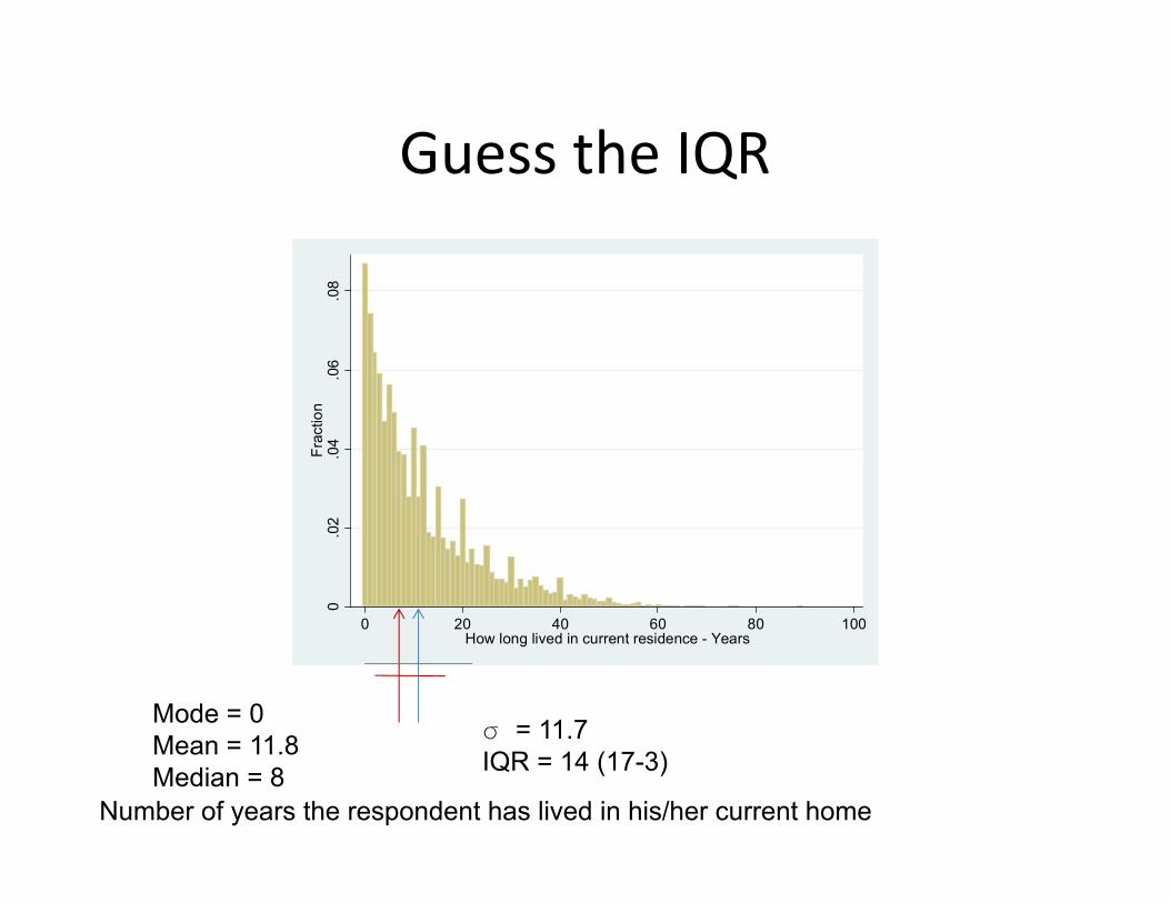
Guess the IQR


0.0

2.0

4.0

6.0

8Fr

actio

n


Mode = 0Mean = 11.8Median = 8

F = 11.7IQR = 14 (17-3)

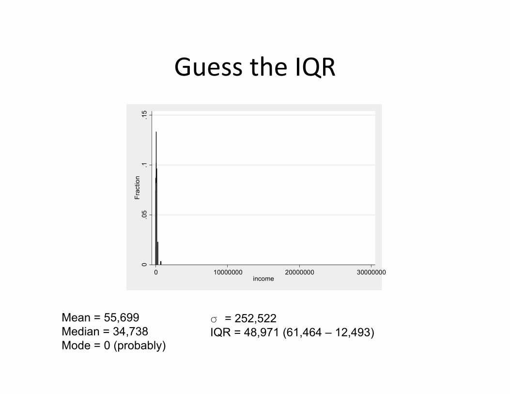
Guess the IQR

0.0

5.1

.15

Frac

tion

0 10000000 20000000 30000000income

Mean = 55,699Median = 34,738Mode = 0 (probably)

F = 252,522IQR = 48,971 (61,464 – 12,493)

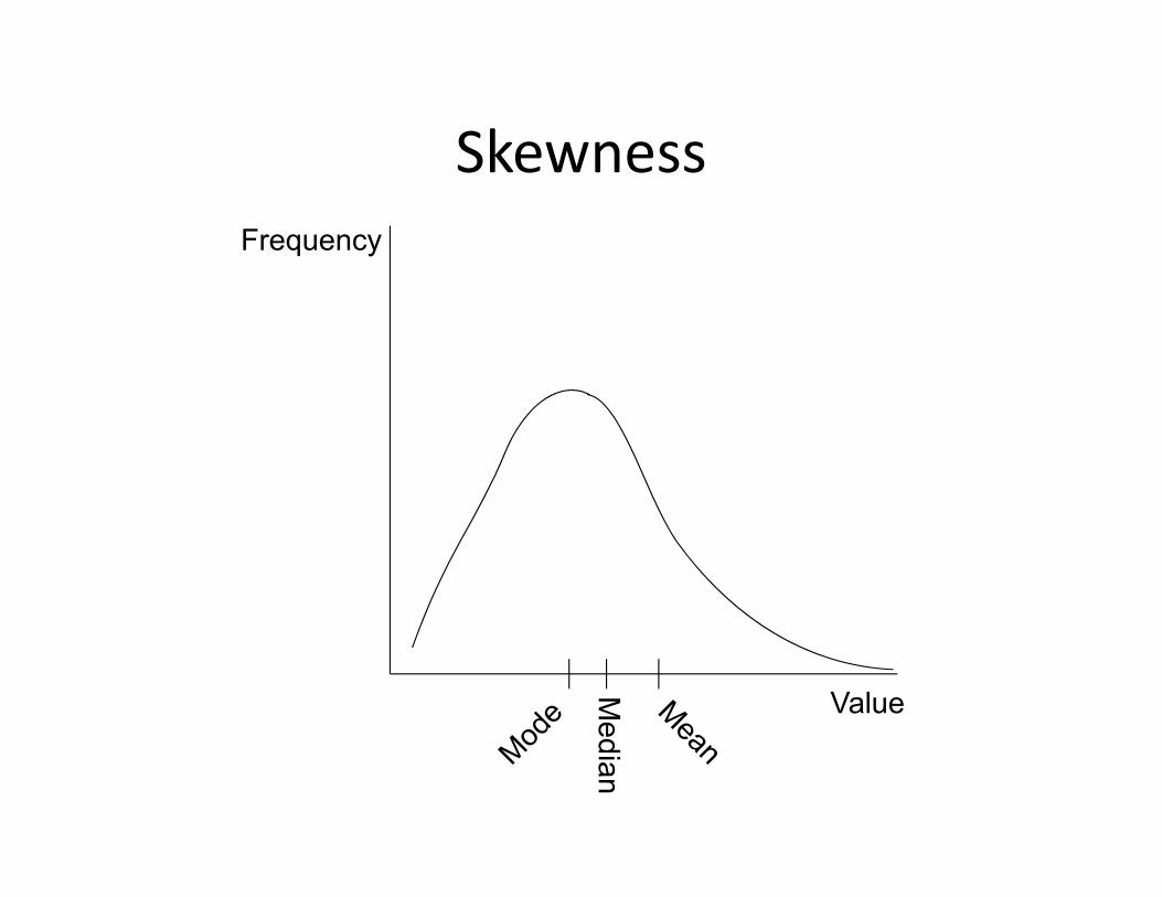
Lopsidedness and peakedness

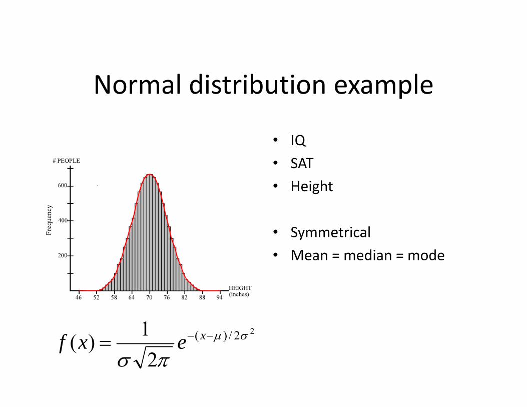
Normal distribution example

• IQ• SAT• Height

• Symmetrical• Mean = median = mode

Value

Frequency

22/)(

21)(

xexf

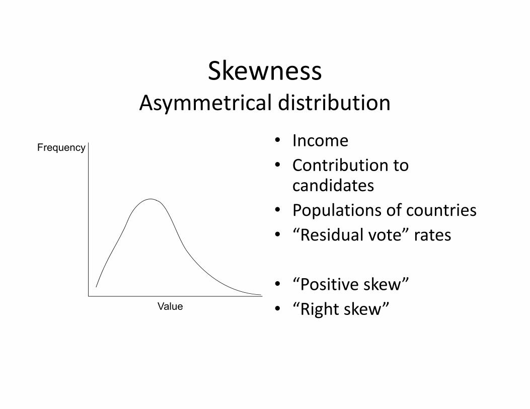
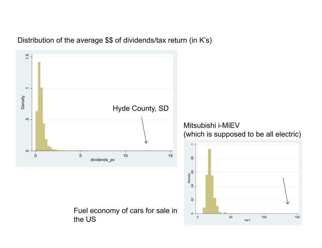
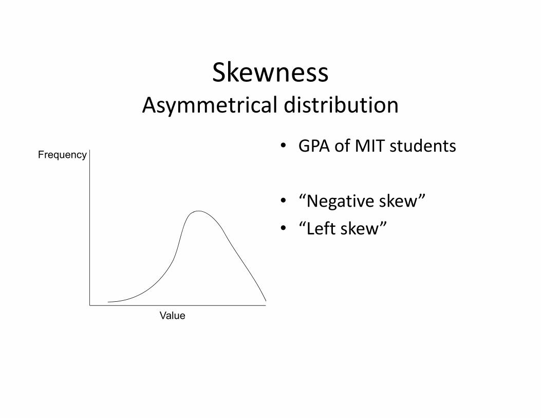
SkewnessAsymmetrical distribution

• Income• Contribution to candidates

• Populations of countries• “Residual vote” rates

• “Positive skew”• “Right skew”Value

Frequency

0.5

11.

5D

ensi

ty

0 5 10 15dividends_pc

Hyde County, SD

Distribution of the average $$ of dividends/tax return (in K’s)

0.0

2.0

4.0

6.0

8.1

Den

sity

0 50 100 150var1

Fuel economy of cars for sale in the US

Mitsubishi i-MiEV(which is supposed to be all electric)

SkewnessAsymmetrical distribution

• GPA of MIT students

• “Negative skew”• “Left skew”

Value

Frequency

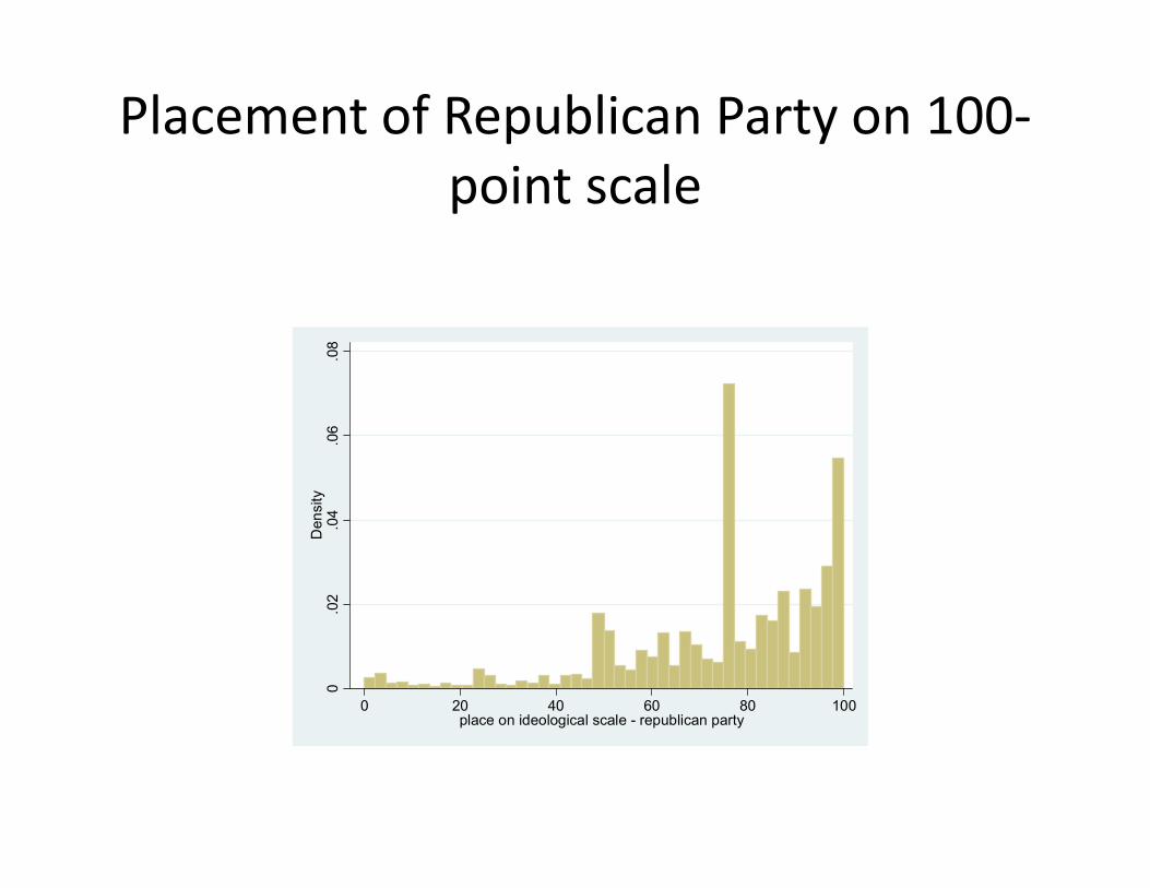
Placement of Republican Party on 100‐point scale

0.0

2.0

4.0

6.0

8D

ensi

ty

0 20 40 60 80 100place on ideological scale - republican party

Skewness

Value

Frequency

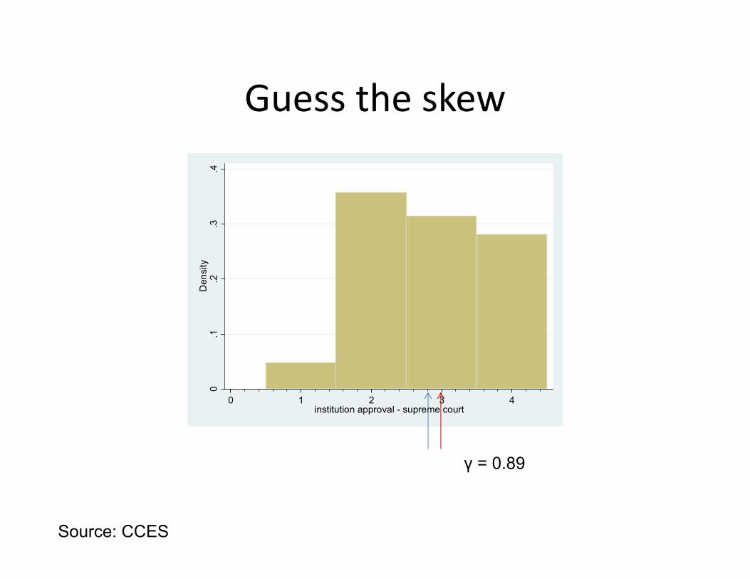
Guess the skew

Source: CCES

0.1

.2.3

.4D

ensi

ty


γ = 0.89

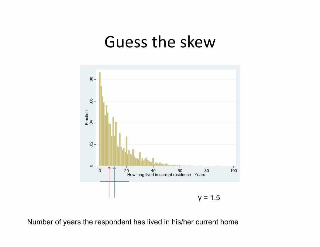
Guess the skew


0.0

2.0

4.0

6.0

8Fr

actio

n


γ = 1.5

Guess the IQR

0.0

5.1

.15

Frac

tion

0 10000000 20000000 30000000income

γ = 91.7

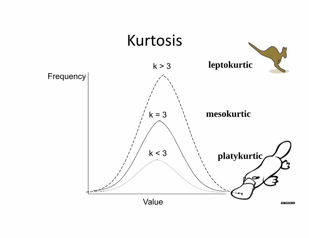
Kurtosis

Value

Frequencyk > 3

k = 3

k < 3

leptokurtic

platykurtic

mesokurtic

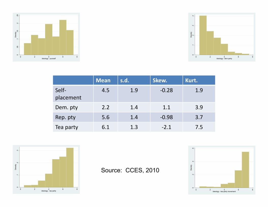
Mean s.d. Skew. Kurt.

Self‐placement

4.5 1.9 ‐0.28 1.9

Dem. pty 2.2 1.4 1.1 3.9

Rep. pty 5.6 1.4 ‐0.98 3.7

Tea party 6.1 1.3 ‐2.1 7.5

Source: CCES, 2010

0.0

5.1

.15

.2.2

5D

ensi

ty

0 2 4 6 8ideology - yourself

0.1

.2.3

.4D

ensi

ty

0 2 4 6 8ideology - dem party

0.1

.2.3

Den

sity

0 2 4 6 8ideology - rep party

0.2

.4.6

Den

sity

0 2 4 6 8ideology - tea party movement

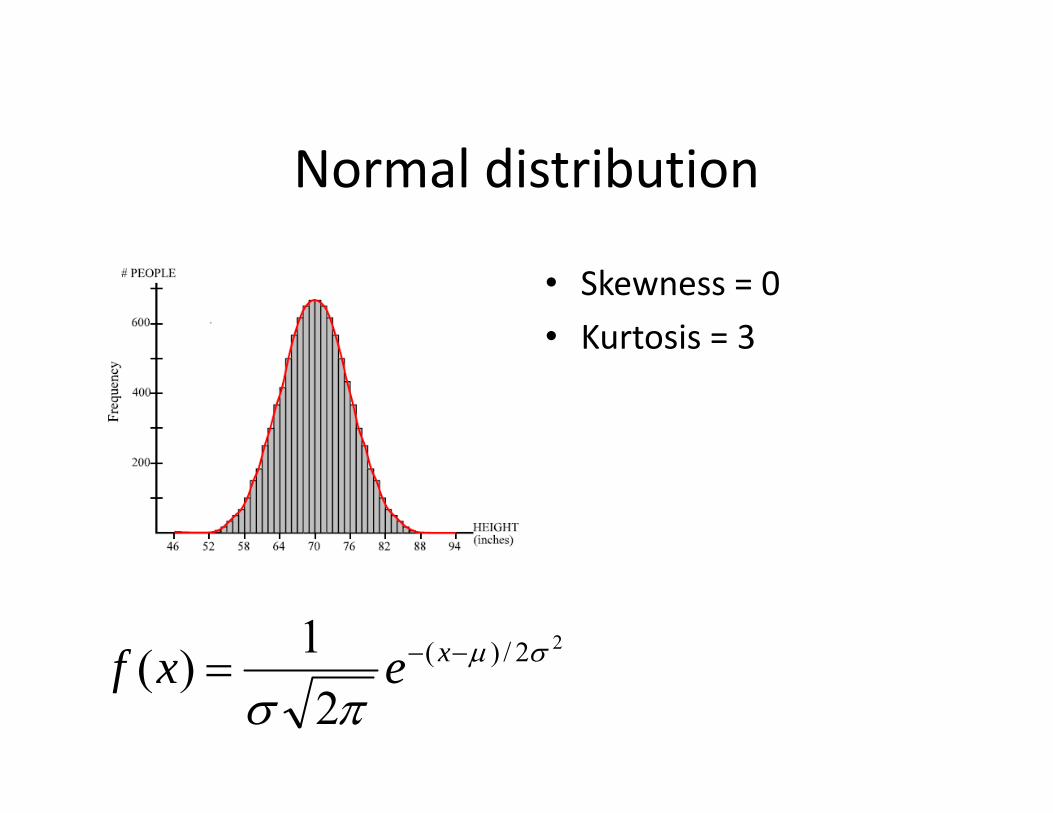
Normal distribution

• Skewness = 0• Kurtosis = 3

22/)(

21)(

xexf

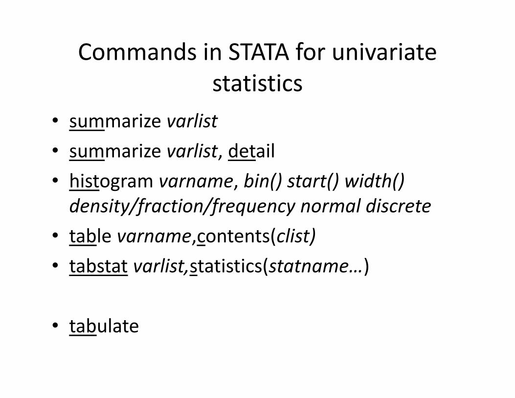
Commands in STATA for univariate statistics

• summarize varlist• summarize varlist, detail• histogram varname, bin() start() width() density/fraction/frequency normal discrete

• table varname,contents(clist)• tabstat varlist,statistics(statname…)

• tabulate

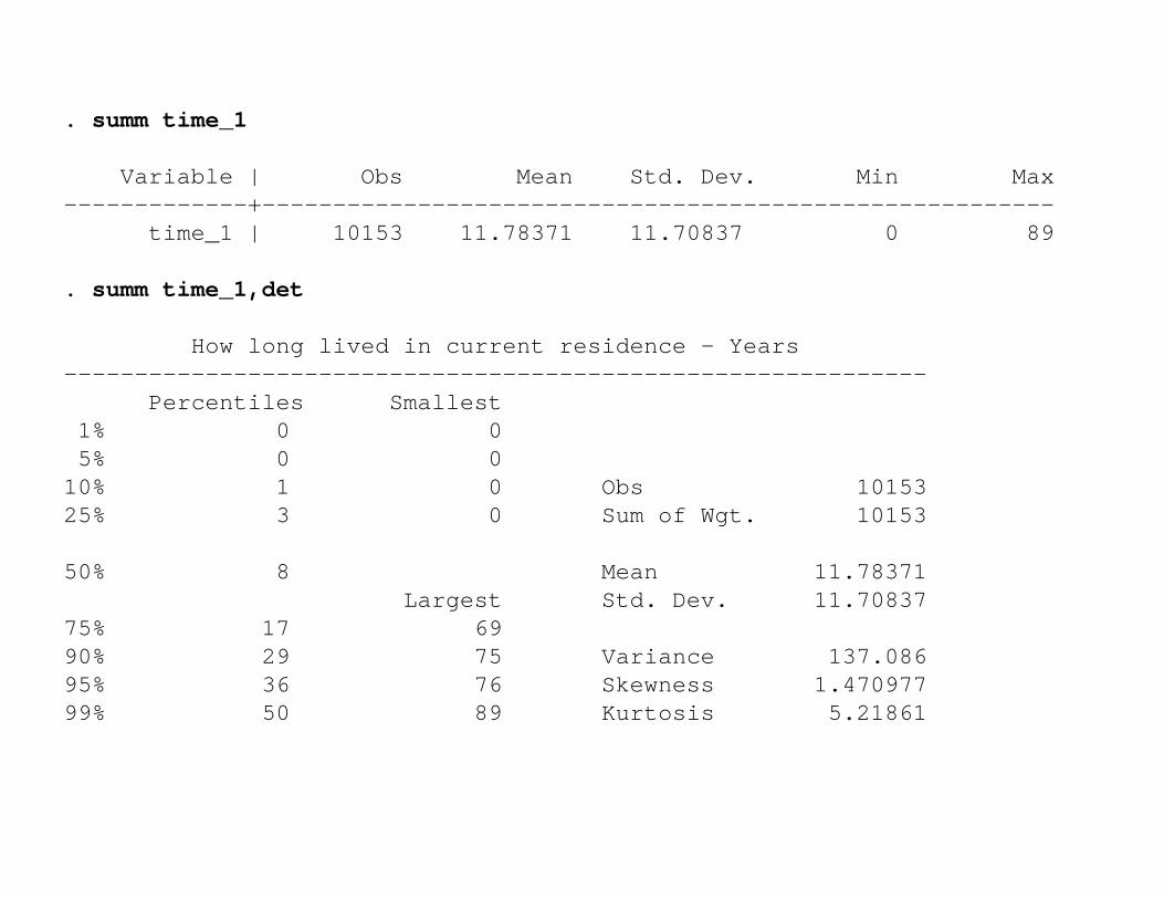
. summ time_1

Variable | Obs Mean Std. Dev. Min Max-------------+--------------------------------------------------------

time_1 | 10153 11.78371 11.70837 0 89

. summ time_1,det

How long lived in current residence - Years-------------------------------------------------------------

Percentiles Smallest1% 0 05% 0 010% 1 0 Obs 1015325% 3 0 Sum of Wgt. 10153

50% 8 Mean 11.78371Largest Std. Dev. 11.70837

75% 17 6990% 29 75 Variance 137.08695% 36 76 Skewness 1.47097799% 50 89 Kurtosis 5.21861

0.0

2.0

4.0

6.0

8D

ensi

ty


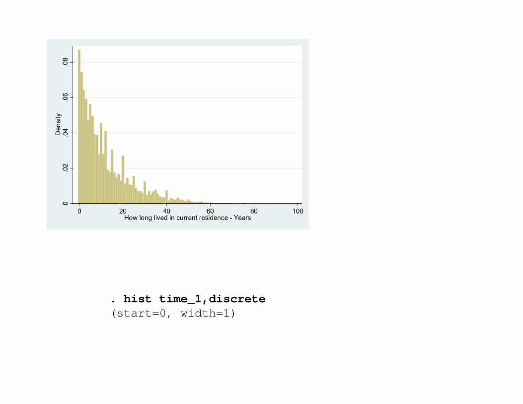
. hist time_1,discrete(start=0, width=1)

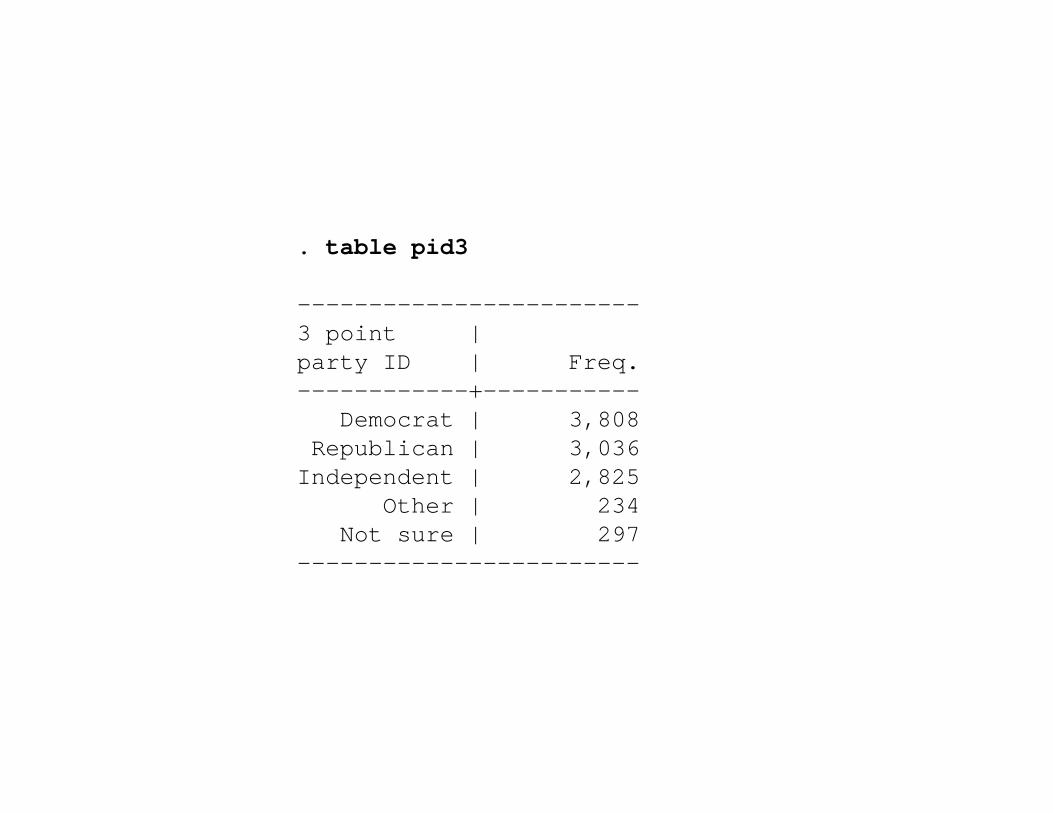
. table pid3

------------------------3 point |party ID | Freq.------------+-----------

Democrat | 3,808Republican | 3,036Independent | 2,825

Other | 234Not sure | 297

------------------------

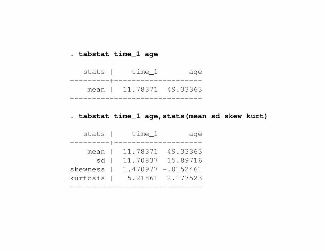
. tabstat time_1 age

stats | time_1 age---------+--------------------

mean | 11.78371 49.33363------------------------------

. tabstat time_1 age,stats(mean sd skew kurt)

stats | time_1 age---------+--------------------

mean | 11.78371 49.33363sd | 11.70837 15.89716

skewness | 1.470977 -.0152461kurtosis | 5.21861 2.177523------------------------------

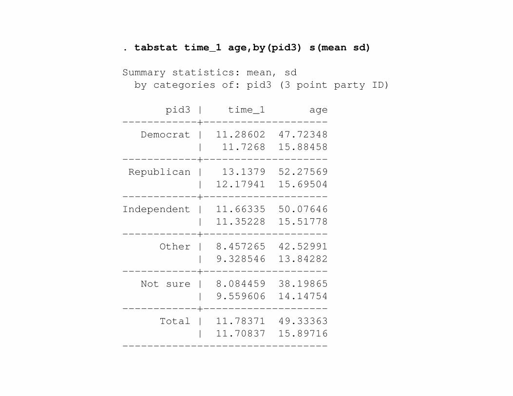
. tabstat time_1 age,by(pid3) s(mean sd)

Summary statistics: mean, sdby categories of: pid3 (3 point party ID)

pid3 | time_1 age------------+--------------------

Democrat | 11.28602 47.72348| 11.7268 15.88458

------------+--------------------Republican | 13.1379 52.27569

| 12.17941 15.69504------------+--------------------Independent | 11.66335 50.07646

| 11.35228 15.51778------------+--------------------

Other | 8.457265 42.52991| 9.328546 13.84282

------------+--------------------Not sure | 8.084459 38.19865

| 9.559606 14.14754------------+--------------------

Total | 11.78371 49.33363| 11.70837 15.89716

---------------------------------

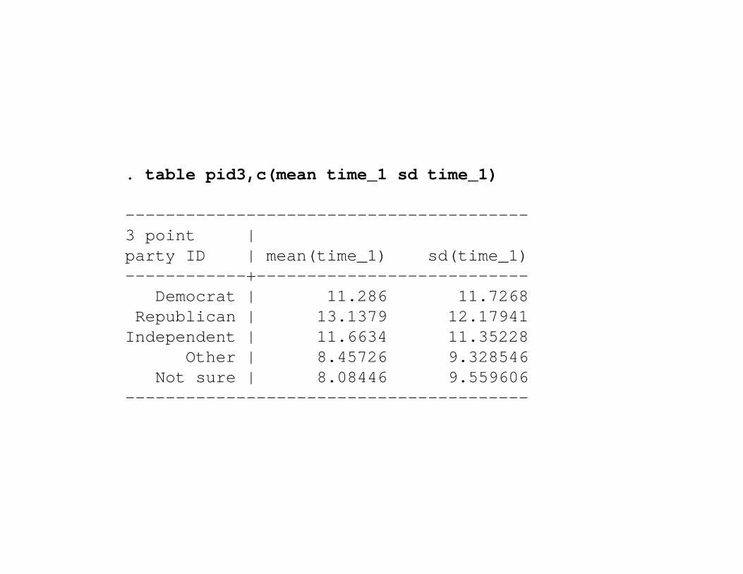
. table pid3,c(mean time_1 sd time_1)

----------------------------------------3 point |party ID | mean(time_1) sd(time_1)------------+---------------------------

Democrat | 11.286 11.7268Republican | 13.1379 12.17941Independent | 11.6634 11.35228

Other | 8.45726 9.328546Not sure | 8.08446 9.559606

----------------------------------------

Univariate graphs

Documents

Introduction to Descriptive Statistics - MIT