2/27/2018

1

ECE 5322 21st Century Electromagnetics

Instructor:Office:Phone:E‐Mail:

Dr. Raymond C. RumpfA‐337(915) 747‐6958rcrumpf@utep.edu

Introduction toEngineered Materials

Lecture #12

Lecture 12 1

Lecture Outline

• Classifications of Engineered Materials• Covered in this Lecture

– Ordinary materials– Nonreciprocal and asymmetric materials and structures– Mixtures

Lecture 12 Slide 2

Aerogel (0.9 mg/cm3)World’s lightest engineered material.

Caltech, University of California Irvine, and HRL Laboratories.

2/27/2018

2

Classification

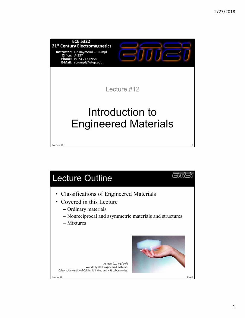
Classifications of Engineered Materials for Electromagnetics

Lecture 12 4

Engineered Materials

Ordinary Materials Mixtures Metamaterials Photonic Crystals

“Pure” materials found in nature or synthesized in the lab.  Based solely on atomic scale phenomena.

• Conductors• Dielectrics• Magnetics• Absorbers• Nonlinear• Anisotropic• Bi• Chiral

Ordinary materials are combined to provide averaged properties.

• Dielectrics• Magnetics• Magneto‐Dielectric• Absorbers

Composite materials designed to provide not observed in the constituent materials.

Resonant• Double Positive• Single Negative• Negative Index• n < 1.0 and  0• Super Absorbers• Nonlinear• Bi• Chiral

Non‐Resonant• Anisotropic• Hyperbolic

Periodic structures where electromagnetic waves behave analogous to electrons in semiconductors.

Band Gap• Complete Band Gap• Partial Band Gap

Dispersive• Self‐Collimating• Negative Refractive• Hyper Dispersive

Nonlinear

Engineered materials are materials that are purposely tailored to exhibit useful and enabling electromagnetic properties.

2/27/2018

3

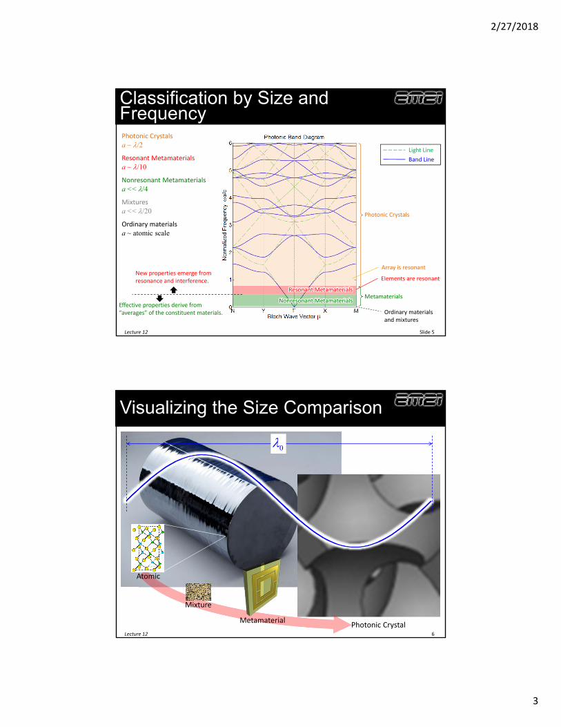
Classification by Size and Frequency

Slide 5Lecture 12

Nonresonant Metamaterials

Resonant Metamaterials

Photonic Crystals

Metamaterials

Ordinary materialsand mixtures

Light Line

Band Line

Photonic Crystalsa ~ /2

Resonant Metamaterialsa ~ /10

Nonresonant Metamaterialsa << /4

Mixturesa << /20

Ordinary materialsa ~ atomic scale

Effective properties derive from “averages” of the constituent materials.

New properties emerge from resonance and interference. Elements are resonant

Array is resonant

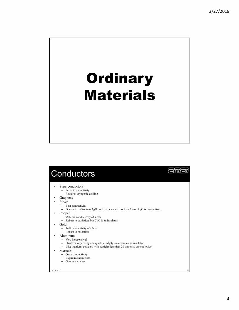
Visualizing the Size Comparison

Lecture 12 6

0

Photonic CrystalMetamaterial

Mixture

Atomic

2/27/2018

4

Ordinary Materials

Conductors• Superconductors

– Perfect conductivity– Requires cryogenic cooling

• Graphene• Silver

– Best conductivity– Does not oxidize into AgO until particles are less than 3 nm. AgO is conductive.

• Copper– 95% the conductivity of silver– Robust to oxidation, but CuO is an insulator.

• Gold– 94% conductivity of silver– Robust to oxidation

• Aluminum– Very inexpensive!– Oxidizes very easily and quickly. Al2O3 is a ceramic and insulator.– Like titanium, powders with particles less than 20 m or so are explosive.

• Mercury– Okay conductivity– Liquid metal mirrors– Gravity switches

Lecture 12 8

2/27/2018

5

Dielectrics

• Teflon– Gold standard for dielectrics (r = 2.1)

• FR4– Common material in printed circuit boards (PCB)

• Water– Water is actually an insulator similar in conductivity to wood.– r = 80 at radio frequencies

• Titanium Dioxide (TiO2)– Excellent thermal stability– r = 100

• Strontium Titanate (SrTiO3)– Very high dielectric constant (r > 300)– Strong temperature dependence

Lecture 12 9

Magnetics• Diamagnetism

– Creates a magnetic field in opposition to an externally applied magnetic field. – Negative susceptibility.– Repelled by magnetic fields.– Very weak phenomenon.– Does not retain magnetism after external field is removed.– Water

• Paramagnetism– Positive susceptibility– Attracted to magnetic fields– Very weak phenomenon– Does not retain magnetism after external field is removed.

• Ferromagnetism– Similar to paramagnetism, but retains magnetism after applied magnetic field is removed.– Strong enough to be felt by hand– Iron, nickel, cobalt, lodestone

• Antiferromagnetism– Transition metal compounds, hematite, chromium, FeMn, and NiO

Lecture 12 10

2/27/2018

6

Absorbers

• Salt water

• Graphite

• Think “black”

Lecture 12 11

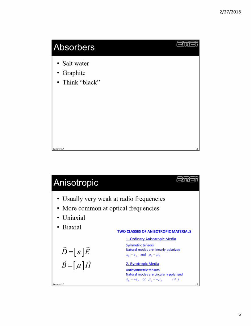
Anisotropic

• Usually very weak at radio frequencies

• More common at optical frequencies

• Uniaxial

• Biaxial

Lecture 12 12

D E

B H

1. Ordinary Anisotropic Media

and ij ji ij ji

Symmetric tensorsNatural modes are linearly polarized

2. Gyrotropic Media

or ij ji ij ji i j

Antisymmetric tensorsNatural modes are circularly polarized

TWO CLASSES OF ANISOTROPIC MATERIALS

2/27/2018

7

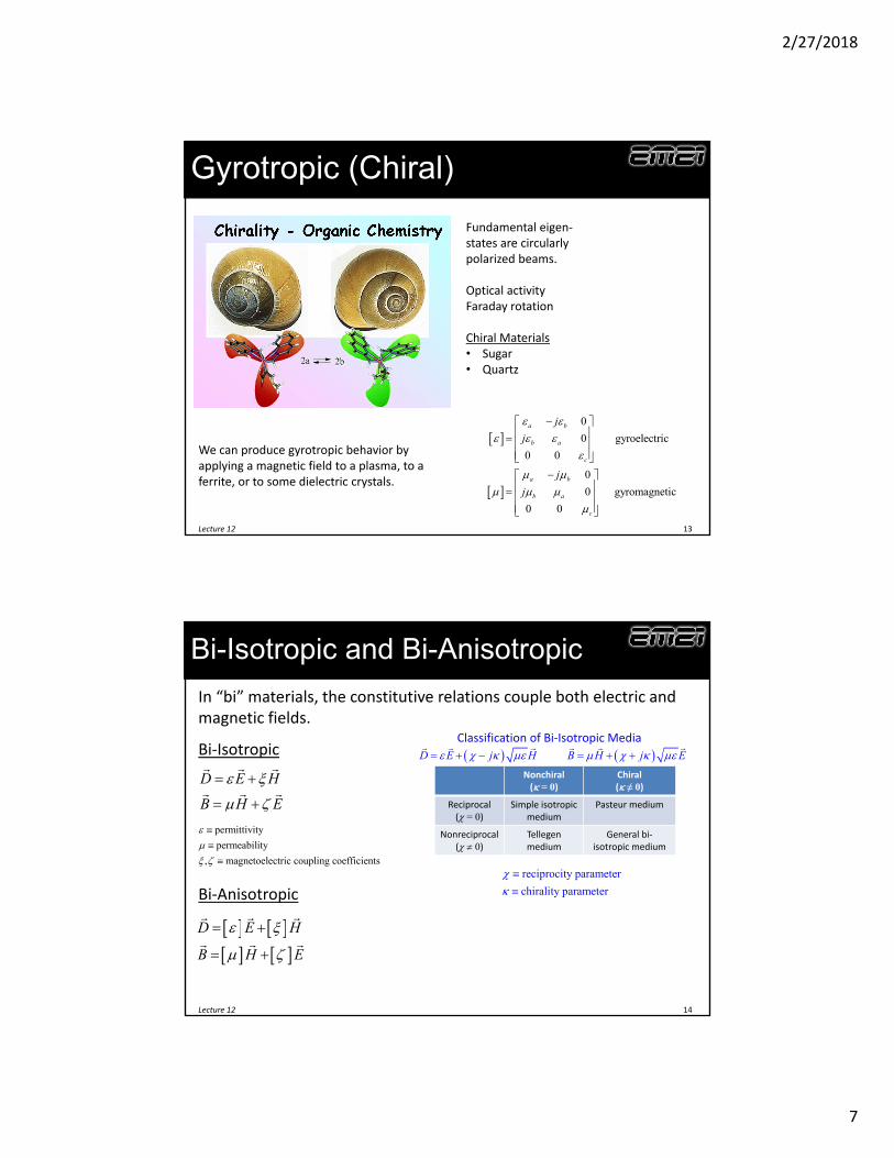
Gyrotropic (Chiral)

Lecture 12 13

Fundamental eigen‐states are circularly polarized beams.

Optical activityFaraday rotation

Chiral Materials• Sugar• Quartz

0

0 gyroelectric

0 0

0

0 gyromagnetic

0 0

a b

b a

c

a b

b a

c

j

j

j

j

We can produce gyrotropic behavior by applying a magnetic field to a plasma, to a ferrite, or to some dielectric crystals.

Bi-Isotropic and Bi-Anisotropic

Lecture 12 14

In “bi” materials, the constitutive relations couple both electric and magnetic fields.

Bi‐Isotropic

D E H

B H E

permittivity

permeability

, magnetoelectric coupling coefficients

D E H

B H E

D E j H B H j E

Nonchiral( = 0)

Chiral( ≠ 0)

Reciprocal( = 0)

Simple isotropic medium

Pasteur medium

Nonreciprocal( 0)

Tellegenmedium

General bi‐isotropic medium

Bi‐Anisotropic

Classification of Bi‐Isotropic Media

reciprocity parameter

chirality parameter

2/27/2018

8

Nonreciprocal & Asymmetric

Materials and Structures

Related, But Easily Confused Phenomena

• Reciprocity

• Asymmetric Devices

• Time-Reversal Symmetry

• Phase Conjugation

Lecture 12 16

2/27/2018

9

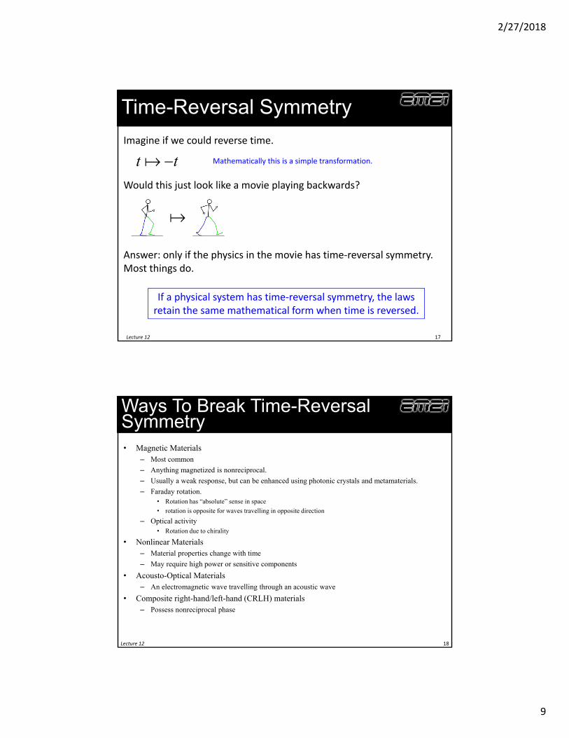
Time-Reversal Symmetry

Lecture 12 17

Imagine if we could reverse time.  

t t Mathematically this is a simple transformation.

Would this just look like a movie playing backwards?

Answer: only if the physics in the movie has time‐reversal symmetry.  Most things do.

If a physical system has time‐reversal symmetry, the laws retain the same mathematical form when time is reversed.

Ways To Break Time-Reversal Symmetry• Magnetic Materials

– Most common

– Anything magnetized is nonreciprocal.

– Usually a weak response, but can be enhanced using photonic crystals and metamaterials.

– Faraday rotation.• Rotation has “absolute” sense in space

• rotation is opposite for waves travelling in opposite direction

– Optical activity• Rotation due to chirality

• Nonlinear Materials– Material properties change with time

– May require high power or sensitive components

• Acousto-Optical Materials– An electromagnetic wave travelling through an acoustic wave

• Composite right-hand/left-hand (CRLH) materials– Possess nonreciprocal phase

Lecture 12 18

2/27/2018

10

Lecture 12 19

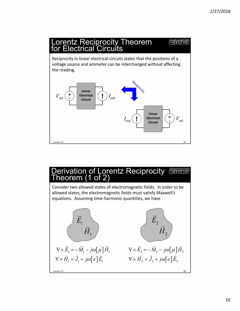
Lorentz Reciprocity Theoremfor Electrical CircuitsReciprocity in linear electrical circuits states that the positions of a voltage source and ammeter can be interchanged without affecting the reading.

Iout+‐Vsrc

LinearElectrical Circuit

Iout+‐ Vsrc

LinearElectrical Circuit

Lecture 12 20

Derivation of Lorentz Reciprocity Theorem (1 of 2)Consider two allowed states of electromagnetic fields.  In order to be allowed states, the electromagnetic fields must satisfy Maxwell’s equations.  Assuming time‐harmonic quantities, we have

1E

1H 2E

2H

1 1 1

1 1 1

E M j H

H J j E

2 2 2

2 2 2

E M j H

H J j E

2/27/2018

11

Lecture 12 21

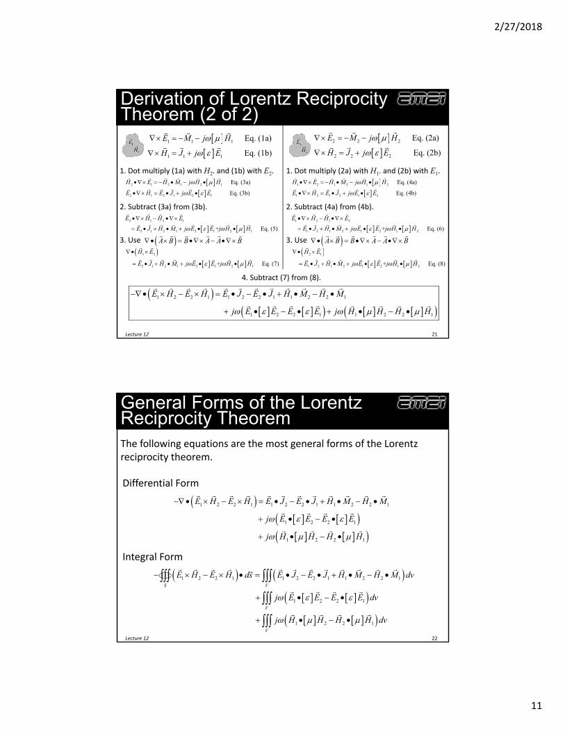
Derivation of Lorentz Reciprocity Theorem (2 of 2)

1. Dot multiply (1a) with H2. and (1b) with E2.

1 1 1

1 1 1

Eq. (1a)

Eq. (1b)

E M j H

H J j E

2 2 2

2 2 2

Eq. (2a)

Eq. (2b)

E M j H

H J j E

2 1 2 1 2 1

2 1 2 1 2 1

Eq. (3a)

Eq. (3b)

H E H M j H H

E H E J j E E

2. Subtract (3a) from (3b).

2 1 2 1

2 1 2 1 2 1 2 1 + Eq. (5)

E H H E

E J H M j E E j H H

3. Use

1 2

2 1 2 1 2 1 2 1 + Eq. (7)

H E

E J H M j E E j H H

A B B A A B

1. Dot multiply (2a) with H1. and (2b) with E1.

1 2 1 2 1 2

1 2 1 2 1 2

Eq. (4a)

Eq. (4b)

H E H M j H H

E H E J j E E

2. Subtract (4a) from (4b).

1 2 1 2

1 2 1 2 1 2 1 2 + Eq. (6)

E H H E

E J H M j E E j H H

3. Use

2 1

1 2 1 2 1 2 1 2 + Eq. (8)

H E

E J H M j E E j H H

A B B A A B

4. Subtract (7) from (8).

1 2 2 1 1 2 2 1 1 2 2 1

1 2 2 1 1 2 2 1

E H E H E J E J H M H M

j E E E E j H H H H

Lecture 12 22

General Forms of the Lorentz Reciprocity Theorem

Differential Form

1 2 2 1 1 2 2 1 1 2 2 1

1 2 2 1

1 2 2 1

E H E H E J E J H M H M

j E E E E

j H H H H

Integral Form

1 2 2 1 1 2 2 1 1 2 2 1

1 2 2 1

1 2 2

S V

V

E H E H ds E J E J H M H M dv

j E E E E dv

j H H H H

1

V

dv

The following equations are the most general forms of the Lorentz reciprocity theorem.

2/27/2018

12

Lecture 12 23

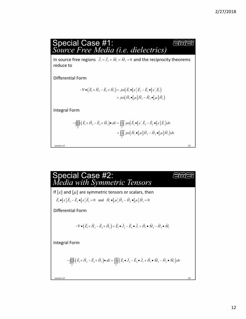
Special Case #1:Source Free Media (i.e. dielectrics)In source free regions                                   and the reciprocity theorems reduce to 

1 2 1 2 0J J M M

Differential Form

1 2 2 1 1 2 2 1

1 2 2 1

E H E H j E E E E

j H H H H

Integral Form

1 2 2 1 1 2 2 1

1 2 2 1

S V

V

E H E H ds j E E E E dv

j H H H H dv

Lecture 12 24

Special Case #2:Media with Symmetric TensorsIf [] and [] are symmetric tensors or scalars, then

1 2 2 1 1 2 2 10 and 0E E E E H H H H

Differential Form

1 2 2 1 1 2 2 1 1 2 2 1E H E H E J E J H M H M

Integral Form

1 2 2 1 1 2 2 1 1 2 2 1

S V

E H E H ds E J E J H M H M dv

2/27/2018

13

Lecture 12 25

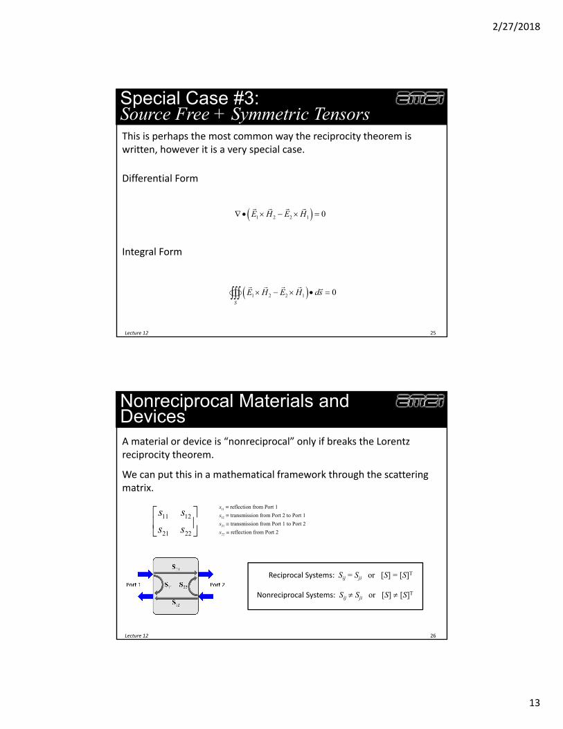
Special Case #3:Source Free + Symmetric TensorsThis is perhaps the most common way the reciprocity theorem is written, however it is a very special case.

Differential Form

1 2 2 1 0E H E H

Integral Form

1 2 2 1 0S

E H E H ds

Nonreciprocal Materials and Devices

Lecture 12 26

A material or device is “nonreciprocal” only if breaks the Lorentz reciprocity theorem.

We can put this in a mathematical framework through the scattering matrix.

11 12

21 22

s s

s s

11

12

21

22

reflection from Port 1

transmission from Port 2 to Port 1

transmission from Port 1 to Port 2

reflection from Port 2

s

s

s

s

Reciprocal Systems:  Sij = Sji or [S] = [S]T

Nonreciprocal Systems:  Sij Sji or [S] [S]T

2/27/2018

14

Lecture 12 27

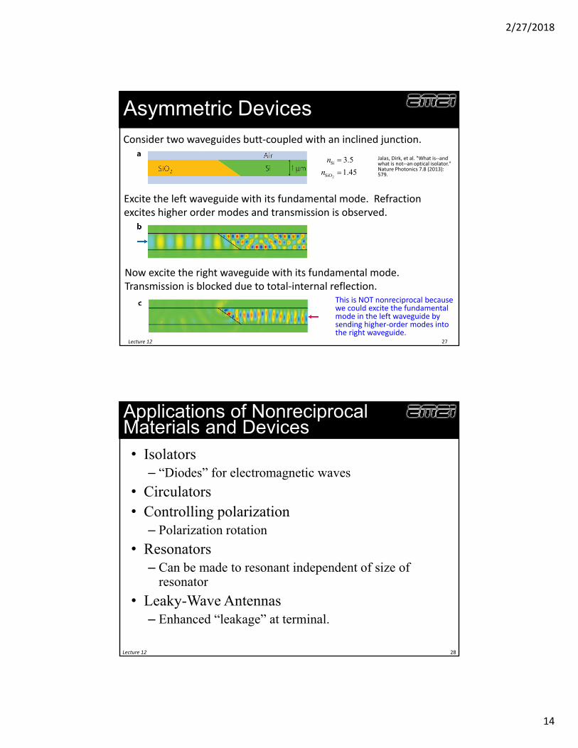
Asymmetric DevicesConsider two waveguides butt‐coupled with an inclined junction.

Excite the left waveguide with its fundamental mode.  Refraction excites higher order modes and transmission is observed.

Now excite the right waveguide with its fundamental mode.  Transmission is blocked due to total‐internal reflection.

2

Si

SiO

3.5

1.45

n

n

This is NOT nonreciprocal because we could excite the fundamental mode in the left waveguide by sending higher‐order modes into the right waveguide.

Jalas, Dirk, et al. "What is‐‐and what is not‐‐an optical isolator." Nature Photonics 7.8 (2013): 579.

Applications of Nonreciprocal Materials and Devices• Isolators

– “Diodes” for electromagnetic waves

• Circulators• Controlling polarization

– Polarization rotation

• Resonators– Can be made to resonant independent of size of

resonator

• Leaky-Wave Antennas– Enhanced “leakage” at terminal.

Lecture 12 28

2/27/2018

15

Nonreciprocal Materials and Devices

• Radio and Microwave Frequencies– Ferrites

– Diodes and transistors

• Optics– Dielectrics based on yttrium iron garnet (YIG)

– Sugar molecules

• Metamaterials– Chiral unit cells

– Unit cells containing nonreciprocal materials

Lecture 12 29

Mixtures

2/27/2018

16

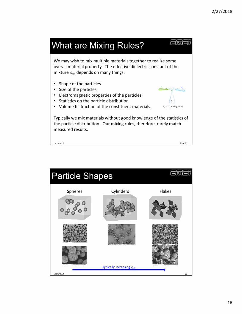
What are Mixing Rules?

Slide 31Lecture 12

We may wish to mix multiple materials together to realize some overall material property.  The effective dielectric constant of the mixture eff depends on many things:

• Shape of the particles• Size of the particles• Electromagnetic properties of the particles.• Statistics on the particle distribution• Volume fill fraction of the constituent materials.

Typically we mix materials without good knowledge of the statistics of the particle distribution.  Our mixing rules, therefore, rarely match measured results.

12

3

3 ? mixing rule

Particle Shapes

Lecture 12 32

Spheres FlakesCylinders

Typically increasing eff

2/27/2018

17

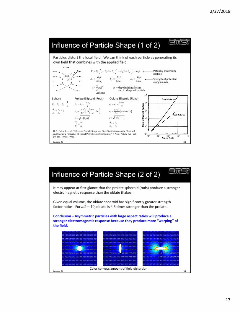
Influence of Particle Shape (1 of 2)

Lecture 12 33

Particles distort the local field.  We can think of each particle as generating its own field that combines with the applied field.

0 0 03 3 3

0 0 0

3

4 4 4

4 depolarizing factors

3

x y z

x y zx y z

i

x y zV S E x S E y S E z

r r rE v E v E v

S S Sn n n

v R n

Sphere1

3

1

x y z

xz

x z

n n n

nS

S n

Prolate Ellipsoid (Rods)

2

3

2

1

2

1 1ln 2

2 1

1

zx y

z

xz

x z

nn n

e en e

e e

e b a

nS

S n

Oblate Ellipsoid (Flake)

21

3

2

1

2

1tan

2

1

zx y

z

xz

x z

nn n

en e e

e

e b a

nS

S n

H. S. Gokturk, et al, “Effects of Particle Shape and Size Distributions on the Electrical and Magnetic Properties of Nickel/Polyethylene Composites,” J. Appl. Polym. Sci., Vol. 50, 1891-1901 (1993).

Potential away from particle

Strength of potential along an axis.

due to shape of particlevolume

Influence of Particle Shape (2 of 2)

Lecture 12 34

It may appear at first glance that the prolate spheroid (rods) produce a stronger electromagnetic response than the oblate (flakes).

Given equal volume, the oblate spheroid has significantly greater strength factor ratios.  For a/b = 10, oblate is 4.5 times stronger than the prolate.

Conclusion – Asymmetric particles with large aspect ratios will produce a stronger electromagnetic response because they produce more “warping” of the field.

Color conveys amount of field distortion

2/27/2018

18

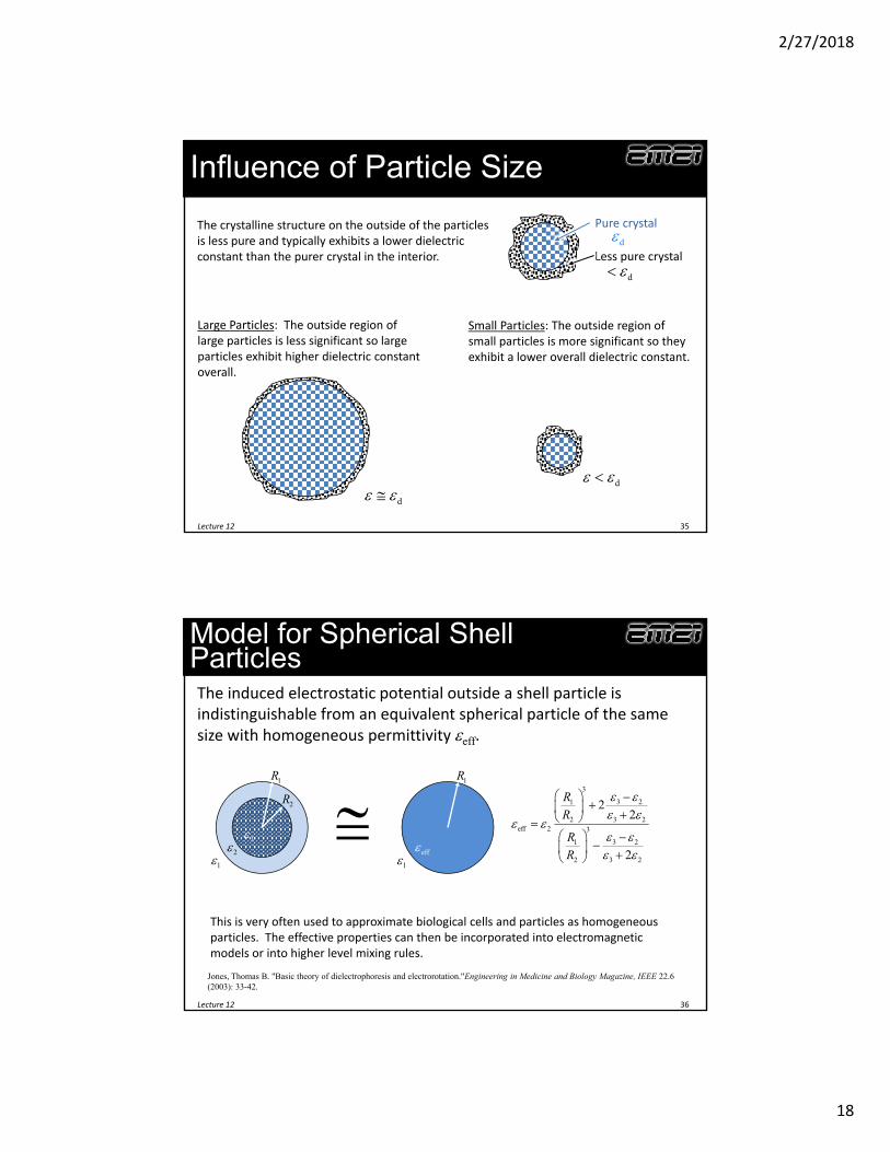
Influence of Particle Size

Lecture 12 35

The crystalline structure on the outside of the particles is less pure and typically exhibits a lower dielectric constant than the purer crystal in the interior.

Pure crystal

Less pure crystald

d

Large Particles:  The outside region of large particles is less significant so large particles exhibit higher dielectric constant overall.

Small Particles: The outside region of small particles is more significant so they exhibit a lower overall dielectric constant.

d d

Model for Spherical Shell Particles

Lecture 12 36

The induced electrostatic potential outside a shell particle is indistinguishable from an equivalent spherical particle of the same size with homogeneous permittivity eff.

1R

2R

21

3

1R

eff1

3

3 21

2 3 2eff 2 3

3 21

2 3 2

22

2

R

R

R

R

This is very often used to approximate biological cells and particles as homogeneous particles.  The effective properties can then be incorporated into electromagnetic models or into higher level mixing rules.

Jones, Thomas B. "Basic theory of dielectrophoresis and electrorotation."Engineering in Medicine and Biology Magazine, IEEE 22.6 (2003): 33-42.

2/27/2018

19

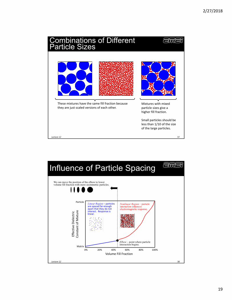
Combinations of Different Particle Sizes

Lecture 12 37

These mixtures have the same fill fraction because they are just scaled versions of each other.

Mixtures with mixed particle sizes give a higher fill fraction.

Small particles should be less than 1/10 of the size of the large particles.

Influence of Particle Spacing

Lecture 12 38

Volume Fill Fraction0% 20% 40% 60% 80% 100%

Effective Dielectric 

Constan

t of Mixture

Matrix

ParticleLinear Region – particles are spaced far enough apart that they do not interact.  Response is linear.

Nonlinear Region – particle interaction enhances electromagnetic response.

Elbow – point where particle interaction begins.

We can move the position of the elbow to lower volume fill fraction with more asymmetric particles.

2/27/2018

20

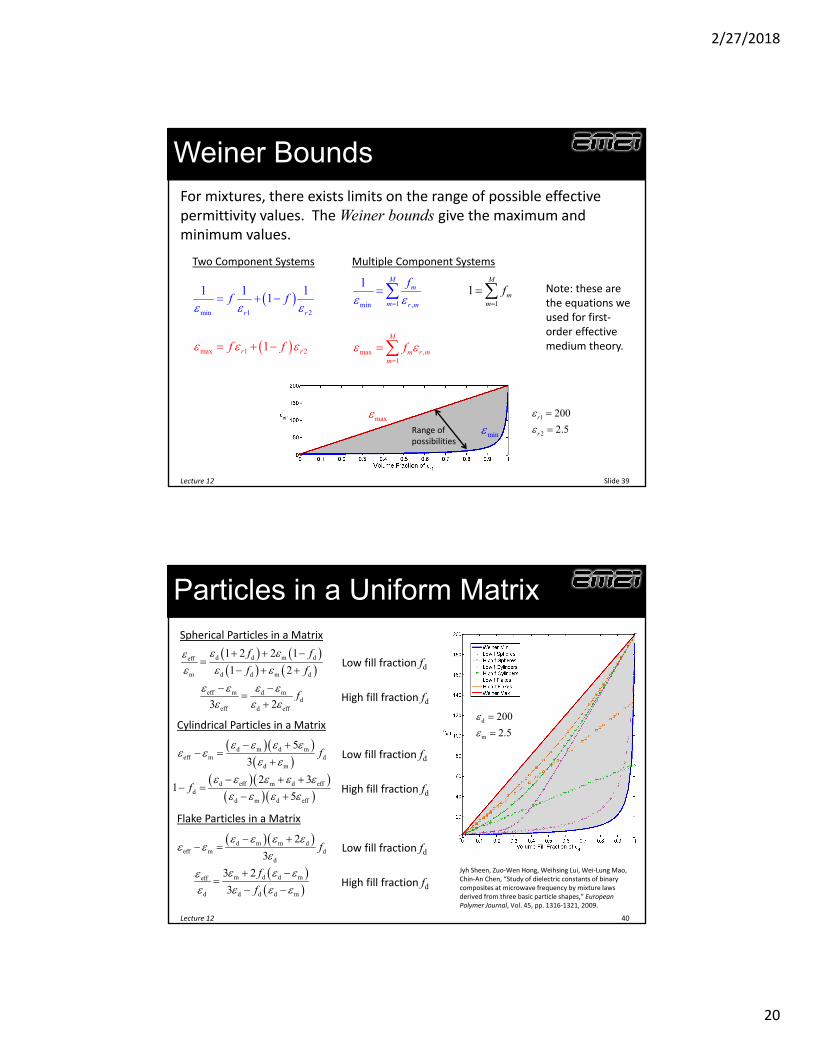
Weiner Bounds

Slide 39Lecture 12

For mixtures, there exists limits on the range of possible effective permittivity values.  The Weiner bounds give the maximum and minimum values.

max

min 1

1 2

2

1 1 1

1

1r r

r r

f f

f f

Two Component Systems

Note: these are the equations we used for first‐order effective medium theory.

1min , 1

max ,1

1

1M

m

m r

M

M

m r mm

mm m

ff

f

Multiple Component Systems

minmax

Range of possibilities

1

2

200

2.5r

r

Particles in a Uniform Matrix

Lecture 12 40

Spherical Particles in a Matrix

d d m deff

m d d m d

1 2 2 1

1 2

f f

f f

Low fill fraction fd

eff m d md

eff d eff3 2f

High fill fraction fd

Cylindrical Particles in a Matrix

d m d meff m d

d m

5

3f

Low fill fraction fd

d eff m d effd

d m d eff

2 31

5f

High fill fraction fd

Flake Particles in a Matrix

d m m deff m d

d

2

3f

Low fill fraction fd

m d d meff

d d d d m

3 2

3

f

f

High fill fraction fd

Jyh Sheen, Zuo‐Wen Hong, Weihsing Lui, Wei‐Lung Mao, Chin‐An Chen, “Study of dielectric constants of binary composites at microwave frequency by mixture laws derived from three basic particle shapes,” European Polymer Journal, Vol. 45, pp. 1316‐1321, 2009.

d

m

200

2.5

2/27/2018

21

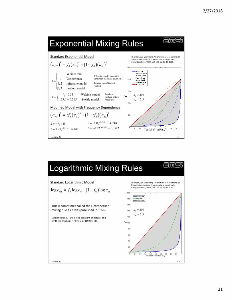
Exponential Mixing Rules

Lecture 12 41

eff d d d m1k k k

f f

1 Weiner min

1 Weiner max

1 2 refractive model

1 3 random model

k

Jyh Sheen, Zuo‐Wen Hong, “Microwave Measurements of Dielectric Constants by Exponential and Logarithmic Mixing Equations,” PIER, Vol. 100, pp. 13‐26, 2010.

Refractive model maintains consistent electrical length nL.

Random model is most realistic.

d

d

0.35 Wakino model

1.65 0.265 Stolzle model

fk

f

Standard Exponential Model

Modified Model with Frequency Dependence

eff d d d m1k k k

zf zf

d

0.04163.23 6.481

k Af B

z f

0.0208

0.0537

11.0 14.748

0.22 1.0582

A f

B f

Random mixture of two materials.

d

m

200

2.5

Logarithmic Mixing Rules

Lecture 12 42

eff d d d mlog log 1 logf f

Jyh Sheen, Zuo‐Wen Hong, “Microwave Measurements of Dielectric Constants by Exponential and Logarithmic Mixing Equations,” PIER, Vol. 100, pp. 13‐26, 2010.

Standard Logarithmic Model

d

m

200

2.5

This is sometimes called the Lichteneckermixing rule as it was published in 1926.

Lichtenecker, K. "Dielectric constant of natural and synthetic mixtures." Phys. Z 27 (1926): 115.

2/27/2018

22

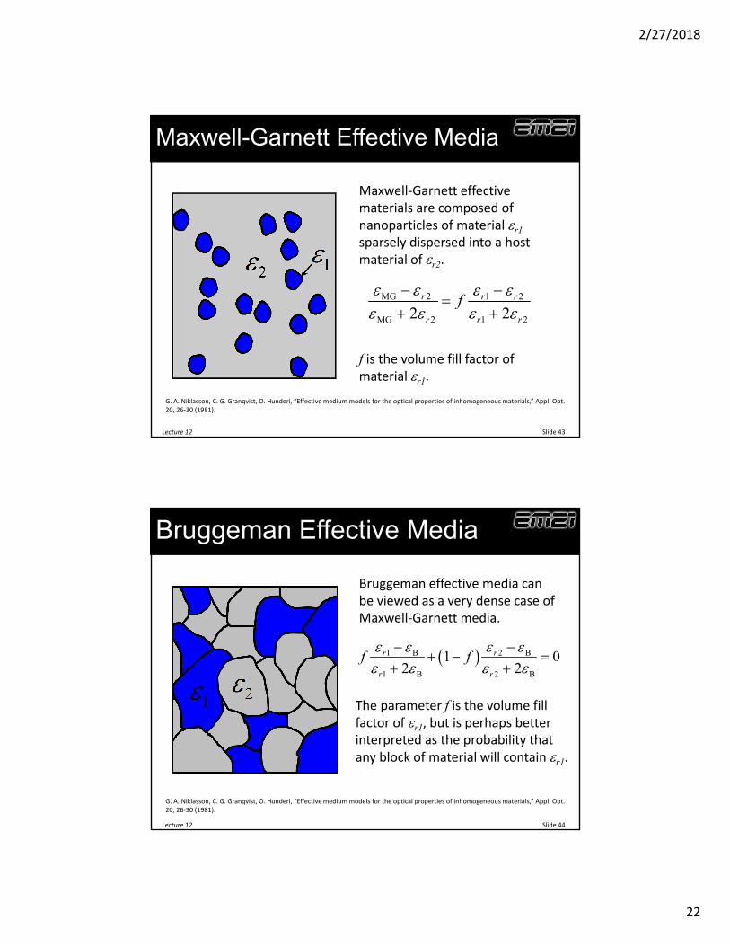
Maxwell-Garnett Effective Media

Slide 43Lecture 12

Maxwell‐Garnett effective materials are composed of nanoparticles of material r1

sparsely dispersed into a host material of r2.

MG 2 1 2

MG 2 1 22 2r r r

r r r

f

f is the volume fill factor of material r1.

G. A. Niklasson, C. G. Granqvist, O. Hunderi, “Effective medium models for the optical properties of inhomogeneous materials,” Appl. Opt. 20, 26‐30 (1981).

Bruggeman Effective Media

Slide 44Lecture 12

Bruggeman effective media can be viewed as a very dense case of Maxwell‐Garnett media.  

1 B 2 B

1 B 2 B

1 02 2

r r

r r

f f

The parameter f is the volume fill factor of r1, but is perhaps better interpreted as the probability that any block of material will contain r1.

G. A. Niklasson, C. G. Granqvist, O. Hunderi, “Effective medium models for the optical properties of inhomogeneous materials,” Appl. Opt. 20, 26‐30 (1981).

2/27/2018

23

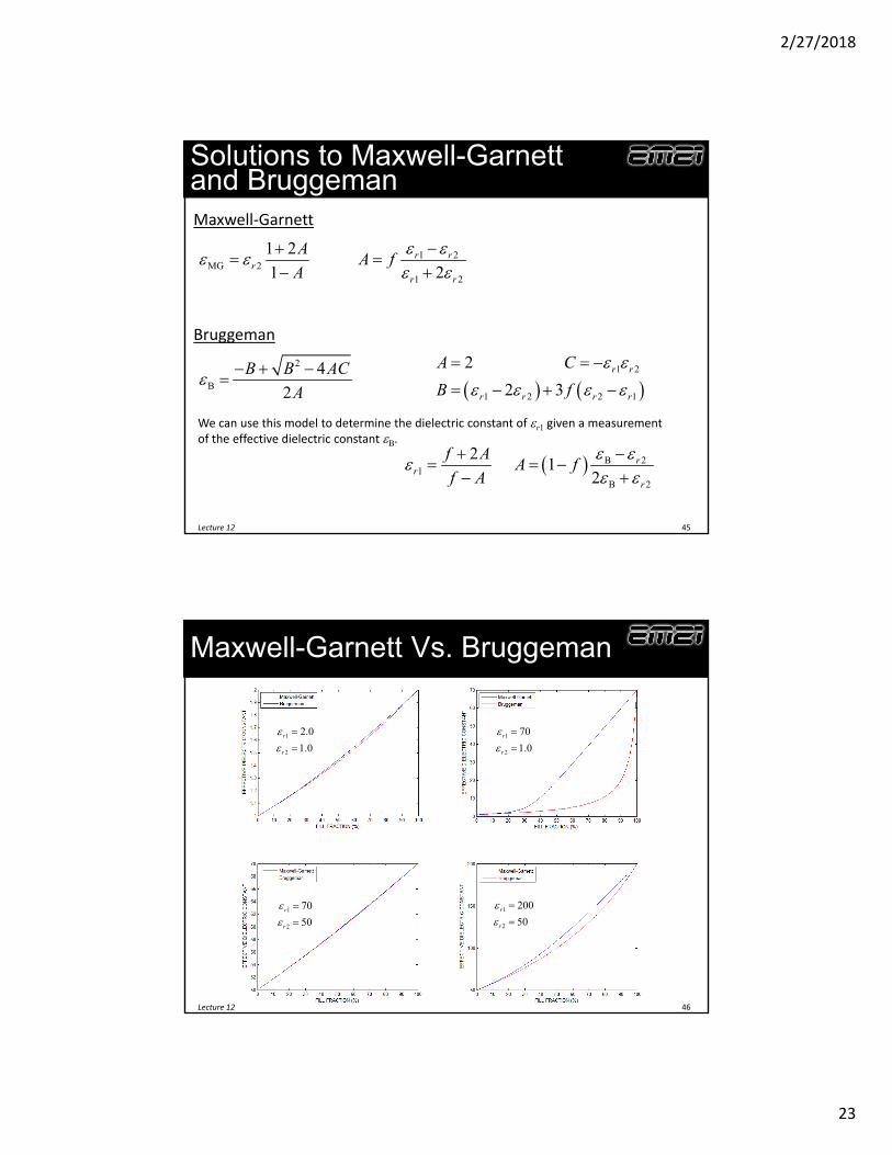
Solutions to Maxwell-Garnett and Bruggeman

Lecture 12 45

Maxwell‐Garnett

1 2MG 2

1 2

1 2

1 2r r

rr r

AA f

A

1 2

1 2 2 1

2

2 3r r

r r r r

A C

B f

Bruggeman

2

B

4

2

B B AC

A

We can use this model to determine the dielectric constant of r1 given a measurement of the effective dielectric constant B.

B 21

B 2

2 1

2r

rr

f AA f

f A

Maxwell-Garnett Vs. Bruggeman

Lecture 12 46

1

2

2.0

1.0r

r

1

2

70

50r

r

1

2

70

1.0r

r

1

2

200

50r

r

2/27/2018

24

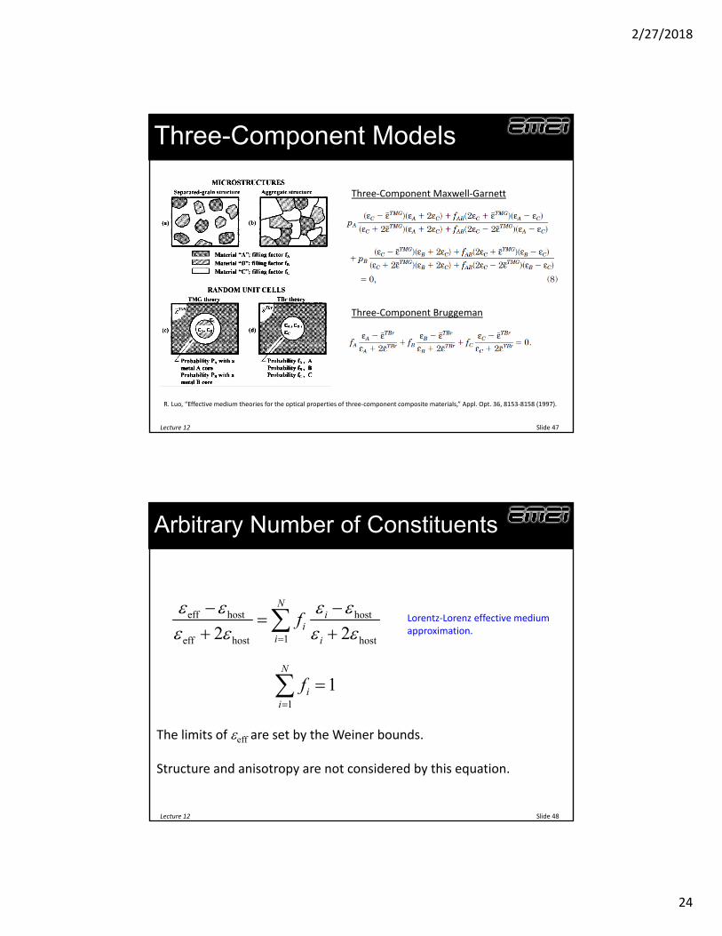
Three-Component Models

Slide 47Lecture 12

R. Luo, “Effective medium theories for the optical properties of three‐component composite materials,” Appl. Opt. 36, 8153‐8158 (1997).

Three‐Component Maxwell‐Garnett

Three‐Component Bruggeman

Arbitrary Number of Constituents

Slide 48Lecture 12

eff host host

1eff host host2 2

Ni

ii i

f

Lorentz‐Lorenz effective medium approximation.

1

1N

ii

f

The limits of eff are set by the Weiner bounds.

Structure and anisotropy are not considered by this equation.