Embed Size (px)
Citation preview
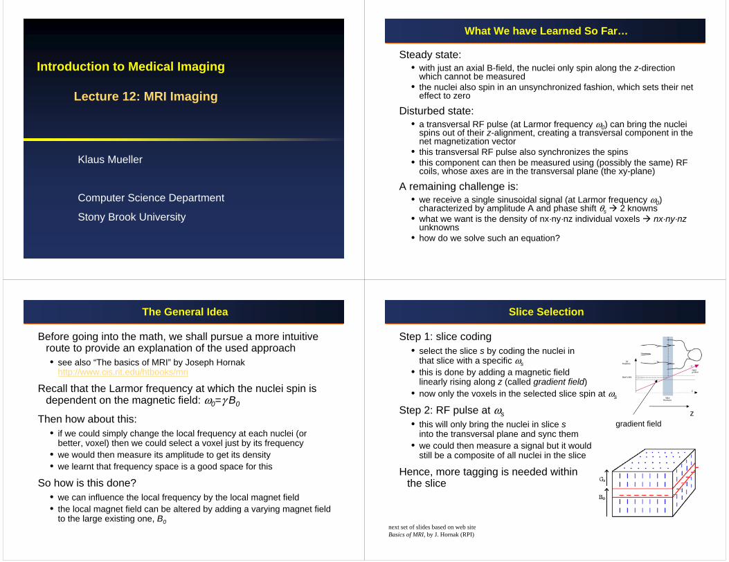
Introduction to Medical Imaging
Lecture 12: MRI Imaging
Klaus Mueller
Computer Science Department
Stony Brook University
What We have Learned So Far…
Steady state:• with just an axial B-field, the nuclei only spin along the z-direction
which cannot be measured • the nuclei also spin in an unsynchronized fashion, which sets their net
effect to zero
Disturbed state:• a transversal RF pulse (at Larmor frequency ω0) can bring the nuclei
spins out of their z-alignment, creating a transversal component in the net magnetization vector
• this transversal RF pulse also synchronizes the spins• this component can then be measured using (possibly the same) RF
coils, whose axes are in the transversal plane (the xy-plane)
A remaining challenge is:• we receive a single sinusoidal signal (at Larmor frequency ω0)
characterized by amplitude A and phase shift θs 2 knowns• what we want is the density of nx·ny·nz individual voxels nx·ny·nz
unknowns• how do we solve such an equation?
The General Idea
Before going into the math, we shall pursue a more intuitive route to provide an explanation of the used approach• see also “The basics of MRI” by Joseph Hornak
http://www.cis.rit.edu/htbooks/mri
Recall that the Larmor frequency at which the nuclei spin is dependent on the magnetic field: ω0=γ B0
Then how about this:• if we could simply change the local frequency at each nuclei (or
better, voxel) then we could select a voxel just by its frequency • we would then measure its amplitude to get its density• we learnt that frequency space is a good space for this
So how is this done?• we can influence the local frequency by the local magnet field• the local magnet field can be altered by adding a varying magnet field
to the large existing one, B0
Slice Selection
Step 1: slice coding• select the slice s by coding the nuclei in
that slice with a specific ωs• this is done by adding a magnetic field
linearly rising along z (called gradient field)• now only the voxels in the selected slice spin at ωs
Step 2: RF pulse at ωs• this will only bring the nuclei in slice s
into the transversal plane and sync them • we could then measure a signal but it would
still be a composite of all nuclei in the slice
Hence, more tagging is needed within the slice
gradient fieldz
next set of slides based on web siteBasics of MRI, by J. Hornak (RPI)
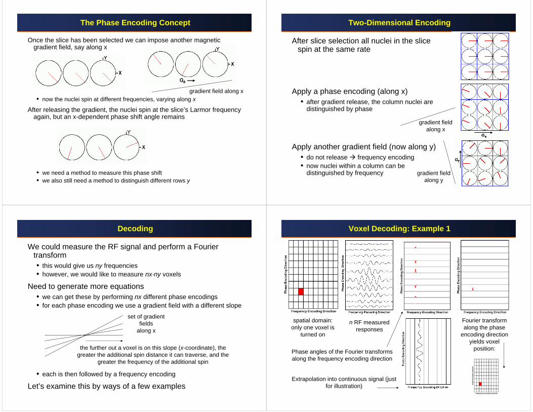
The Phase Encoding Concept
Once the slice has been selected we can impose another magnetic gradient field, say along x
• now the nuclei spin at different frequencies, varying along x
After releasing the gradient, the nuclei spin at the slice’s Larmor frequency again, but an x-dependent phase shift angle remains
• we need a method to measure this phase shift• we also still need a method to distinguish different rows y
gradient field along x
Two-Dimensional Encoding
After slice selection all nuclei in the slice spin at the same rate
Apply a phase encoding (along x)• after gradient release, the column nuclei are
distinguished by phase
Apply another gradient field (now along y)• do not release frequency encoding• now nuclei within a column can be
distinguished by frequency
gradient field along x
gradient field along y
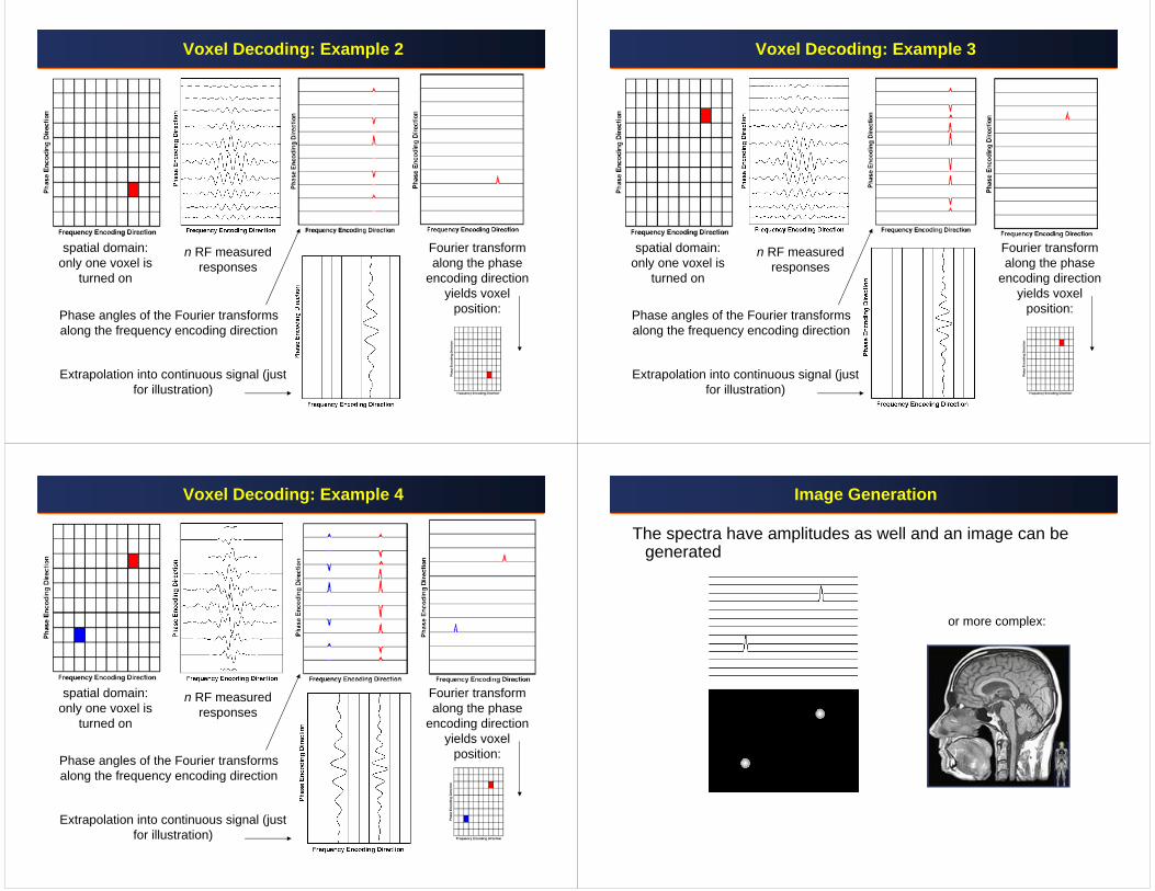
Decoding
We could measure the RF signal and perform a Fourier transform• this would give us ny frequencies• however, we would like to measure nx·ny voxels
Need to generate more equations• we can get these by performing nx different phase encodings• for each phase encoding we use a gradient field with a different slope
• each is then followed by a frequency encoding
Let’s examine this by ways of a few examples
set of gradient fields
along x
the further out a voxel is on this slope (x-coordinate), the greater the additional spin distance it can traverse, and the
greater the frequency of the additional spin
Voxel Decoding: Example 1
spatial domain: only one voxel is
turned on
n RF measured responses
Phase angles of the Fourier transforms along the frequency encoding direction
Extrapolation into continuous signal (just for illustration)
Fourier transform along the phase
encoding direction yields voxel
position:
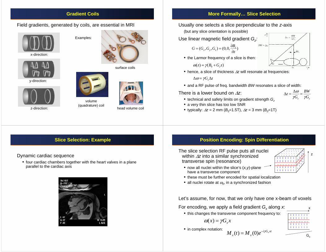
Voxel Decoding: Example 2
spatial domain: only one voxel is
turned on
n RF measured responses
Phase angles of the Fourier transforms along the frequency encoding direction
Extrapolation into continuous signal (just for illustration)
Fourier transform along the phase
encoding direction yields voxel
position:
Voxel Decoding: Example 3
spatial domain: only one voxel is
turned on
n RF measured responses
Phase angles of the Fourier transforms along the frequency encoding direction
Extrapolation into continuous signal (just for illustration)
Fourier transform along the phase
encoding direction yields voxel
position:
Voxel Decoding: Example 4
spatial domain: only one voxel is
turned on
n RF measured responses
Phase angles of the Fourier transforms along the frequency encoding direction
Extrapolation into continuous signal (just for illustration)
Fourier transform along the phase
encoding direction yields voxel
position:
Image Generation
The spectra have amplitudes as well and an image can be generated
or more complex:
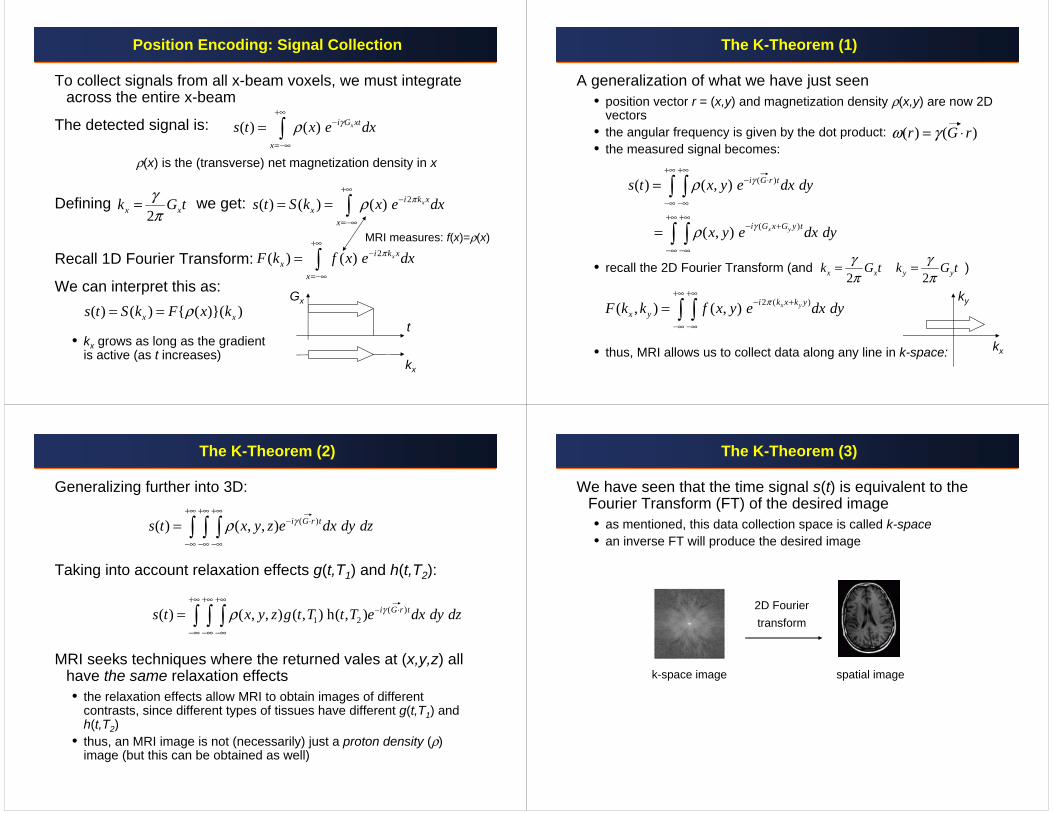
Gradient Coils
Field gradients, generated by coils, are essential in MRI
x-direction:
y-direction:
z-direction:
surface coils
volume (quadrature) coil
head volume coil
Examples:
More Formally… Slice Selection
Usually one selects a slice perpendicular to the z-axis(but any slice orientation is possible)
Use linear magnetic field gradient Gz:
• the Larmor frequency of a slice is then:
• hence, a slice of thickness Δz will resonate at frequencies:
• and a RF pulse of freq. bandwidth BW resonates a slice of width:
There is a lower bound on Δz:• technical and safety limits on gradient strength Gz• a very thin slice has too low SNR• typically: Δz = 2 mm (B0=1.5T), Δz = 3 mm (B0=1T)
( , , ) (0,0, )zx y z
BG G G Gz
∂= =∂
0( ) ( )zz B G zω γ= +
zG zω γΔ = Δ
z z
BWzG Gω
γ γΔΔ = =
Slice Selection: Example
Dynamic cardiac sequence• four cardiac chambers together with the heart valves in a plane
parallel to the cardiac axis
Position Encoding: Spin Differentiation
The slice selection RF pulse puts all nuclei within Δz into a similar synchronized transverse spin (resonance)• now all nuclei within the slice’s (x,y)-plane
have a transverse component• these must be further encoded for spatial localization• all nuclei rotate at ω0, in a synchronized fashion
Let’s assume, for now, that we only have one x-beam of voxels
For encoding, we apply a field gradient Gx along x:• this changes the transverse component frequency to:
• in complex notation:
( ) xx G xω γ=
( ) (0) xi G xtx xM t M e γ−= Gx
z
x
Position Encoding: Signal Collection
To collect signals from all x-beam voxels, we must integrate across the entire x-beam
The detected signal is:
ρ(x) is the (transverse) net magnetization density in x
Defining we get:
Recall 1D Fourier Transform:
We can interpret this as:
• kx grows as long as the gradient is active (as t increases)
( ) ( ) xi G xt
x
s t x e dxγρ+∞
−
=−∞
= ∫
2x xk G tγπ
= 2( ) ( ) ( ) xi k xx
x
s t S k x e dxπρ+∞
−
=−∞
= = ∫
2( ) ( ) xi k xx
x
F k f x e dxπ+∞
−
=−∞
= ∫
( ) ( ) { ( )}( )x xs t S k F x kρ= =t
Gx
kx
MRI measures: f(x)=ρ(x)
The K-Theorem (1)
A generalization of what we have just seen• position vector r = (x,y) and magnetization density ρ(x,y) are now 2D
vectors • the angular frequency is given by the dot product:• the measured signal becomes:
• recall the 2D Fourier Transform (and )
• thus, MRI allows us to collect data along any line in k-space:
( ) ( )r G rω γ= ⋅
( )
( )
( ) ( , )
( , ) x y
i G r t
i G x G y t
s t x y e dx dy
x y e dx dy
γ
γ
ρ
ρ
+∞ +∞− ⋅
−∞ −∞+∞ +∞
− +
−∞ −∞
=
=
∫ ∫
∫ ∫
2 ( )( , ) ( , ) x yi k x k yx yF k k f x y e dx dyπ
+∞ +∞− +
−∞ −∞
= ∫ ∫
2 2x x y yk G t k G tγ γπ π
= =
kx
ky
The K-Theorem (2)
Generalizing further into 3D:
Taking into account relaxation effects g(t,T1) and h(t,T2):
MRI seeks techniques where the returned vales at (x,y,z) all have the same relaxation effects• the relaxation effects allow MRI to obtain images of different
contrasts, since different types of tissues have different g(t,T1) and h(t,T2)
• thus, an MRI image is not (necessarily) just a proton density (ρ) image (but this can be obtained as well)
( )1 2( ) ( , , ) ( , ) h( , ) i G r ts t x y z g t T t T e dx dy dzγρ
+∞ +∞ +∞− ⋅
−∞ −∞ −∞
= ∫ ∫ ∫
( )( ) ( , , ) i G r ts t x y z e dx dy dzγρ+∞ +∞ +∞
− ⋅
−∞ −∞ −∞
= ∫ ∫ ∫
The K-Theorem (3)
We have seen that the time signal s(t) is equivalent to the Fourier Transform (FT) of the desired image• as mentioned, this data collection space is called k-space• an inverse FT will produce the desired image
k-space image spatial image
2D Fourier transform
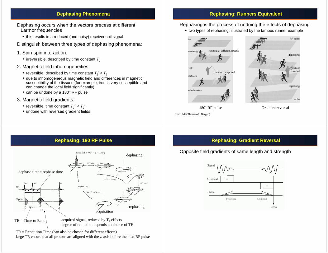
Dephasing Phenomena
Dephasing occurs when the vectors precess at different Larmor frequencies• this results in a reduced (and noisy) receiver coil signal
Distinguish between three types of dephasing phenomena:
1. Spin-spin interaction: • irreversible, described by time constant T2
2. Magnetic field inhomogeneities:• reversible, described by time constant T2
* < T2• due to inhomogeneous magnetic field and differences in magnetic
susceptibility of the tissues (for example, iron is very susceptible and can change the local field significantly)
• can be undone by a 180° RF pulse
3. Magnetic field gradients: • reversible, time constant T2
*” < T2*
• undone with reversed gradient fields
Rephasing: Runners Equivalent
Rephasing is the process of undoing the effects of dephasing• two types of rephasing, illustrated by the famous runner example
180˚ RF pulse Gradient reversal
running at different speeds
runners transposed
from: Frits Thorsen (U Bergen)
Rephasing: 180 RF Pulse
acquired signal, reduced by T2 effectsdegree of reduction depends on choice of TE
dephasing
rephasingacquisition
TE = Time to Echo
TR = Repetition Time (can also be chosen for different effects)large TR ensure that all protons are aligned with the z-axis before the next RF pulse
dephase time= rephase time
Rephasing: Gradient Reversal
Opposite field gradients of same length and strength
The Art of Choosing TR and TE
TR and TE can be varied to bring out proton density (PD), T1, and T2 properties of the tissue
Recall the Bloch relaxation formula:where Mxy0 is the transversal component at t=0
MRI seeks to bring out tissue contrast as manifested by differences in PD, T1, or T2 properties (T1/TR, T2/TE ratios)• choose TE and TR according to the T1 and T2 constants of the target
and adjacent tissues• pick the imaging protocol that brings out these contrasts best• this is called T1, T2, PD weighting
1 20 (1- )
TR TET T
xy xyM M e e− −
=
T1 T2
TR TR
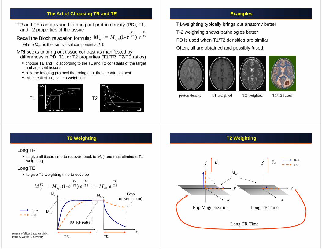
Examples
proton density T1-weighted T2-weighted
T1-weighting typically brings out anatomy better
T-2 weighting shows pathologies better
PD is used when T1/T2 densities are similar
Often, all are obtained and possibly fused
T1/T2 fused
Long TR• to give all tissue time to recover (back to Mz0) and thus eliminate T1
weighting
Long TE• to give T2 weighting time to develop
Mz
TRt t
TE
Mxy
T2 Weighting
2 1 2 20 0 (1- )
TR TE TET T T Txy xy zM M e e M e
− − −= ⇒
t
90˚ RF pulse
Mzo
Echo(measurement)
next set of slides based on slidesfrom: S. Wayte (U Coventry)
Brain
CSF
T2 Weighting
z
y
x
B0 z
y
x
B0
Flip Magnetization Long TE Time
Long TR Time
Brain
CSF
Mxy
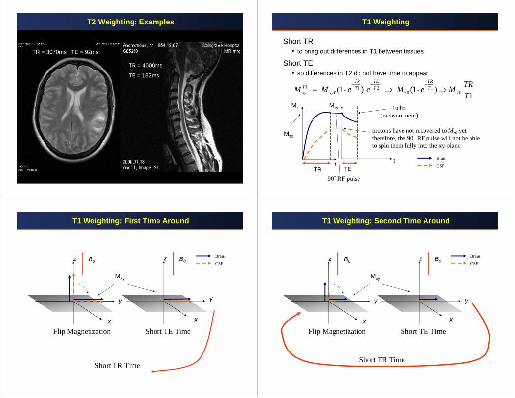
T2 Weighting: Examples
TR = 3070ms TE = 92ms
TR = 4000ms
TE = 132ms
TRt t
TE
T1 Weighting
Short TR• to bring out differences in T1 between tissues
Short TE• so differences in T2 do not have time to appear
1 1 2 10 0 0 (1- ) (1- )
1
TR TE TRT T T Txy xy z z
TRM M e e M e MT
− − −= ⇒ ⇒
Mz Mxy
protons have not recovered to Mz0 yettherefore, the 90˚ RF pulse will not be able to spin them fully into the xy-plane
Mzo
90˚ RF pulse
Echo(measurement)
Brain
CSF
T1 Weighting: First Time Around
z
y
x
B0 z
y
x
B0
Flip Magnetization Short TE Time
Short TR Time
Brain
CSF
Mxy
T1 Weighting: Second Time Around
z
y
x
B0 z
y
x
B0
Flip Magnetization Short TE Time
Short TR Time
Brain
CSF
Mxy
T1 Weighting: All Subsequent Rounds
z
y
x
B0 z
y
x
B0
Flip Magnetization Short TE Time
Short TR Time
Brain
CSF
Mxy
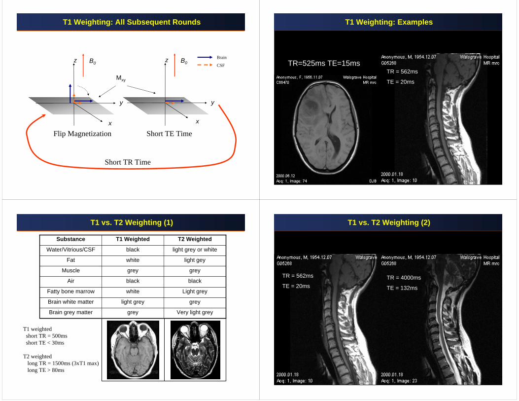
T1 Weighting: Examples
TR = 562ms
TE = 20ms
TR=525ms TE=15ms
T1 vs. T2 Weighting (1)
grey
light grey
white
black
grey
white
black
T1 Weighted
Very light greyBrain grey matter
greyBrain white matter
Light greyFatty bone marrow
blackAir
greyMuscle
light geyFat
light grey or whiteWater/Vitrious/CSF
T2 WeightedSubstance
T1 weightedshort TR = 500ms short TE < 30ms
T2 weighted long TR = 1500ms (3xT1 max)long TE > 80ms
T1 vs. T2 Weighting (2)
TR = 562ms
TE = 20msTR = 4000ms
TE = 132ms
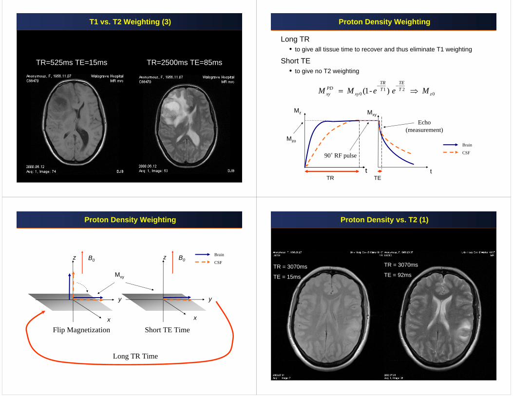
T1 vs. T2 Weighting (3)
TR=525ms TE=15ms TR=2500ms TE=85ms
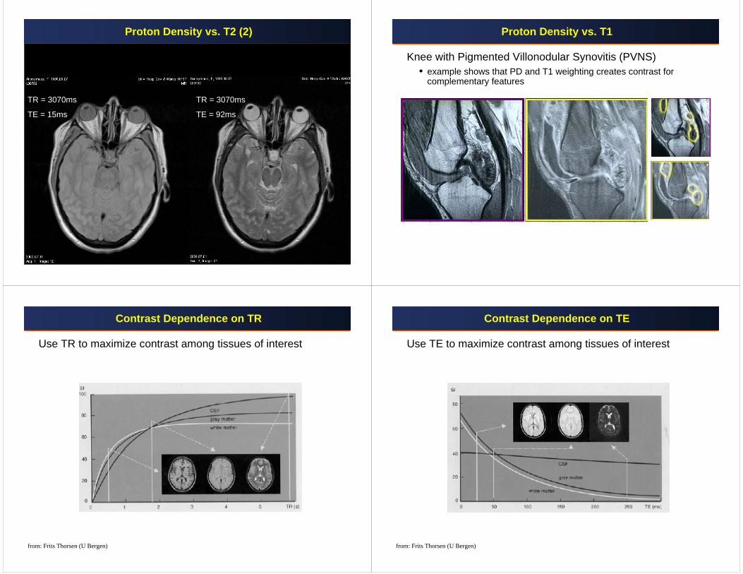
Proton Density Weighting
Long TR• to give all tissue time to recover and thus eliminate T1 weighting
Short TE• to give no T2 weighting
1 20 0 (1- )
TR TEPD T Txy xy zM M e e M
− −= ⇒
Mz
t t
Mxy
t
90˚ RF pulse
Mzo
Echo(measurement)
TRt
TE
Brain
CSF
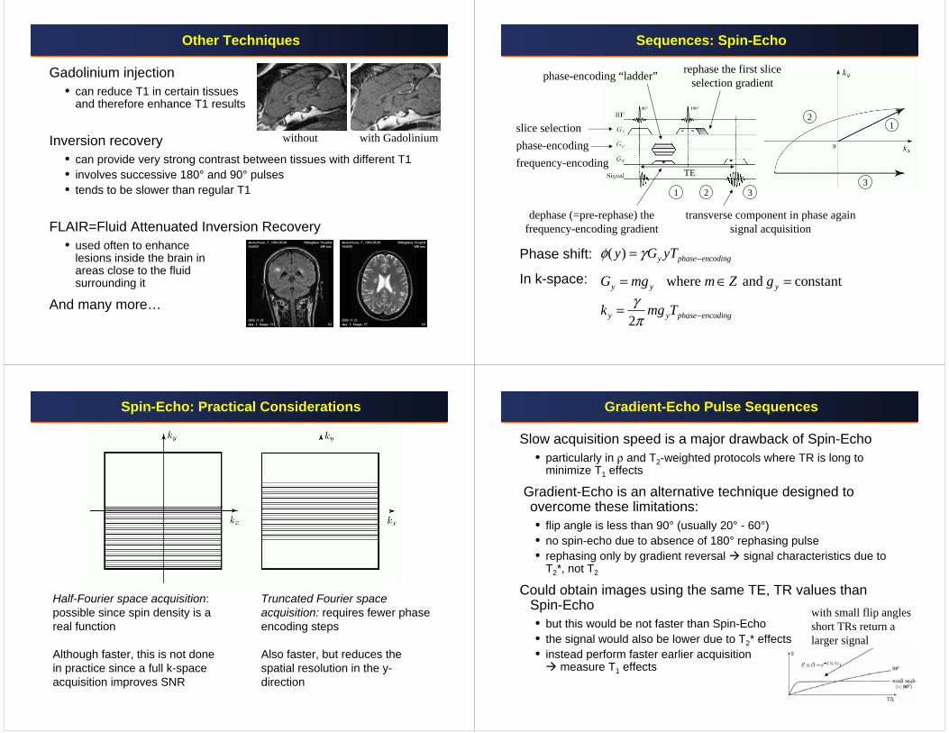
Proton Density Weighting
z
y
x
B0 z
y
x
B0
Flip Magnetization Short TE Time
Long TR Time
Brain
CSF
Mxy
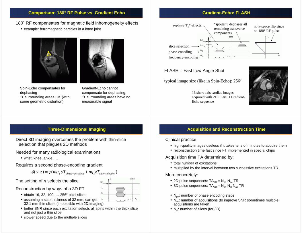
Proton Density vs. T2 (1)
TR = 3070ms
TE = 15ms
TR = 3070ms
TE = 92ms
Proton Density vs. T2 (2)
TR = 3070ms
TE = 15ms
TR = 3070ms
TE = 92ms
Proton Density vs. T1
Knee with Pigmented Villonodular Synovitis (PVNS)• example shows that PD and T1 weighting creates contrast for
complementary features
Contrast Dependence on TR
Use TR to maximize contrast among tissues of interest
from: Frits Thorsen (U Bergen)
Contrast Dependence on TE
Use TE to maximize contrast among tissues of interest
from: Frits Thorsen (U Bergen)
Other Techniques
Gadolinium injection• can reduce T1 in certain tissues
and therefore enhance T1 results
Inversion recovery• can provide very strong contrast between tissues with different T1• involves successive 180° and 90° pulses• tends to be slower than regular T1
FLAIR=Fluid Attenuated Inversion Recovery• used often to enhance
lesions inside the brain in areas close to the fluid surrounding it
And many more…
without with Gadolinium
Sequences: Spin-Echo
Phase shift:
In k-space:
rephase the first slice selection gradient
slice selection phase-encoding frequency-encoding
phase-encoding “ladder”
transverse component in phase againsignal acquisition
dephase (=pre-rephase) the frequency-encoding gradient
12
31 2 3
TE
( ) y phase encodingy G yTφ γ −=
where and constanty y yG mg m Z g= ∈ =
2y y phase encodingk mg Tγπ −=
Spin-Echo: Practical Considerations
Half-Fourier space acquisition: possible since spin density is a real function
Although faster, this is not done in practice since a full k-space acquisition improves SNR
Truncated Fourier space acquisition: requires fewer phase encoding steps
Also faster, but reduces the spatial resolution in the y-direction
Gradient-Echo Pulse Sequences
Slow acquisition speed is a major drawback of Spin-Echo• particularly in ρ and T2-weighted protocols where TR is long to
minimize T1 effects
Gradient-Echo is an alternative technique designed to overcome these limitations:• flip angle is less than 90° (usually 20° - 60°)• no spin-echo due to absence of 180° rephasing pulse• rephasing only by gradient reversal signal characteristics due to
T2*, not T2
Could obtain images using the same TE, TR values than Spin-Echo• but this would be not faster than Spin-Echo• the signal would also be lower due to T2* effects• instead perform faster earlier acquisition
measure T1 effects
with small flip angles short TRs return a larger signal
Comparison: 180° RF Pulse vs. Gradient Echo
180˚ RF compensates for magnetic field inhomogeneity effects• example: ferromagnetic particles in a knee joint
Spin-Echo compensates for dephasing
surrounding areas OK (with some geometric distortion)
Gradient-Echo cannot compensate for dephasing:
surrounding areas have no measurable signal
Gradient-Echo: FLASH
FLASH = Fast Low Angle Shot
slice selection phase-encoding frequency-encoding
“spoiler”: dephases all remaining transverse components
rephase T2* effects no k-space flip since no 180° RF pulse
16 short axis cardiac images acquired with 2D FLASH Gradient-Echo sequence
typical image size (like in Spin-Echo): 2562
Three-Dimensional Imaging
Direct 3D imaging overcomes the problem with thin-slice selection that plagues 2D methods
Needed for many radiological examinations• wrist, knee, ankle, …
Requires a second phase-encoding gradient
The setting of n selects the slice
Reconstruction by ways of a 3D FT• obtain 16, 32, 100, … 2562 pixel slices• assuming a slab thickness of 32 mm, can get
32 1 mm thin slices (impossible with 2D imaging) • better SNR since each excitation selects all spins within the thick slice
and not just a thin slice • slower speed due to the multiple slices
( , ) ( )y phase encoding z slab selectiony z mg yT ng zTφ γ − −= +
Acquisition and Reconstruction Time
Clinical practice: • high-quality images useless if it takes tens of minutes to acquire them• reconstruction time fast since FT implemented in special chips
Acquisition time TA determined by:• total number of excitations• multiplied by the interval between two successive excitations TR
More concretely:• 2D pulse sequences: TA2D = Nph Nac TR• 3D pulse sequences: TA3D = Nph Nsl Nac TR
• Nph: number of phase encoding steps• Nac: number of acquisitions (to improve SNR sometimes multiple
acquisitions are taken)• Nsl: number of slices (for 3D)
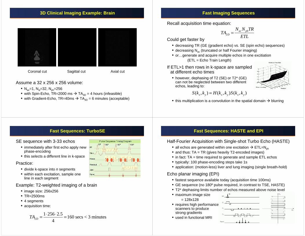
3D Clinical Imaging Example: Brain
Coronal cut Sagittal cut Axial cut
Assume a 32 x 256 x 256 volume:• Nac=1, Nsl=32, Nph=256• with Spin-Echo, TR=2000 ms TA3D = 4 hours (infeasible)• with Gradient-Echo, TR=40ms TA3D = 6 minutes (acceptable)
Fast Imaging Sequences
Recall acquisition time equation:
Could get faster by• decreasing TR (GE (gradient echo) vs. SE (spin echo) sequences)• decreasing Nac (truncated or half Fourier imaging)• or…generate and acquire multiple echos in one excitiation
(ETL = Echo Train Length)
If ETL>1 then rows in k-space are sampled at different echo times• however, dephasing of T2 (SE) or T2* (GE)
can not be neglected between two different echos, leading to:
• this multiplication is a convolution in the spatial domain blurring
2ac ph
D
N N TRTA
ETL=
( , ) ( , ) ( , )x y x y x yS k k H k k S k k=
Fast Sequences: TurboSE
SE sequence with 3-33 echos• immediately after first echo apply new
phase-encoding• this selects a different line in k-space
Practice:• divide k-space into n segments• within each excitation, sample one
line in each segment
Example: T2-weighted imaging of a brain• image size: 256x256• TR=2500ms• 4 segments• acquisition time:
21 256 2.5 160 secs < 3 minutes
4DTA ⋅ ⋅= =
Fast Sequences: HASTE and EPI
Half-Fourier Acquisition with Single-shot Turbo Echo (HASTE)• all echos are generated within one excitation ETL=Nph• and thus: TA = TR (gives heavily T2-encoded images)• in fact: TA = time required to generate and sample ETL echos• typically: 100 phase-encoding steps take 1s• application: (motion-less) liver and lung imaging (single breath-hold)
Echo planar imaging (EPI)• fastest sequence available today (acquisition time 100ms)• GE sequence (no 180º pulse required, in contrast to TSE, HASTE)• T2* dephasing limits number of echos measured above noise level• maximum image size
= 128x128• requires high performance
scanners to produce strong gradients
• used in functional MRI
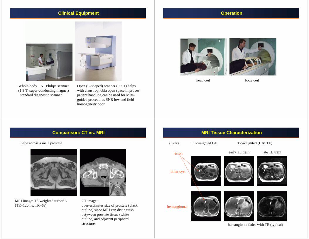
Clinical Equipment
Whole-body 1.5T Philips scanner (1.5 T, super-conducting magnet)standard diagnostic scanner
Open (C-shaped) scanner (0.2 T) helps with claustrophobia open space improves patient handling can be used for MRI-guided procedures SNR low and field homogeneity poor
Operation
head coil body coil
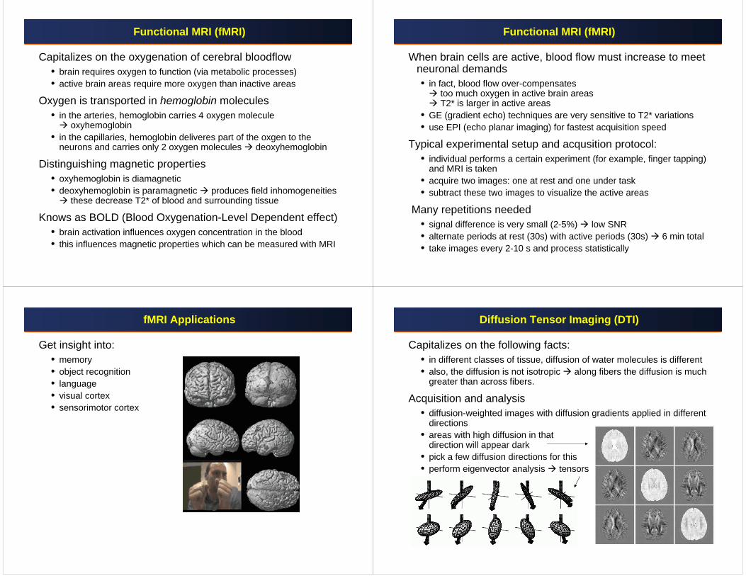
Comparison: CT vs. MRI
Slice across a male prostate
MRI image: T2-weighted turboSE(TE=120ms, TR=6s)
CT image:over-estimates size of prostate (black outline) since MRI can distinguish betyween prostate tissue (white outline) and adjacent peripheral structures
MRI Tissue Characterization
T1-weighted GE T2-weighted (HASTE)
early TE train late TE train
biliar cyst
hemangioma
lesion
hemangioma fades with TE (typical)
(liver)
Functional MRI (fMRI)
Capitalizes on the oxygenation of cerebral bloodflow• brain requires oxygen to function (via metabolic processes)• active brain areas require more oxygen than inactive areas
Oxygen is transported in hemoglobin molecules• in the arteries, hemoglobin carries 4 oxygen molecule
oxyhemoglobin• in the capillaries, hemoglobin deliveres part of the oxgen to the
neurons and carries only 2 oxygen molecules deoxyhemoglobin
Distinguishing magnetic properties• oxyhemoglobin is diamagnetic• deoxyhemoglobin is paramagnetic produces field inhomogeneities
these decrease T2* of blood and surrounding tissue
Knows as BOLD (Blood Oxygenation-Level Dependent effect)• brain activation influences oxygen concentration in the blood• this influences magnetic properties which can be measured with MRI
Functional MRI (fMRI)
When brain cells are active, blood flow must increase to meet neuronal demands• in fact, blood flow over-compensates
too much oxygen in active brain areas T2* is larger in active areas
• GE (gradient echo) techniques are very sensitive to T2* variations• use EPI (echo planar imaging) for fastest acquisition speed
Typical experimental setup and acqusition protocol:• individual performs a certain experiment (for example, finger tapping)
and MRI is taken• acquire two images: one at rest and one under task• subtract these two images to visualize the active areas
Many repetitions needed• signal difference is very small (2-5%) low SNR• alternate periods at rest (30s) with active periods (30s) 6 min total• take images every 2-10 s and process statistically
fMRI Applications
Get insight into:• memory• object recognition• language• visual cortex• sensorimotor cortex
Diffusion Tensor Imaging (DTI)
Capitalizes on the following facts:• in different classes of tissue, diffusion of water molecules is different• also, the diffusion is not isotropic along fibers the diffusion is much
greater than across fibers.
Acquisition and analysis• diffusion-weighted images with diffusion gradients applied in different
directions • areas with high diffusion in that
direction will appear dark• pick a few diffusion directions for this• perform eigenvector analysis tensors
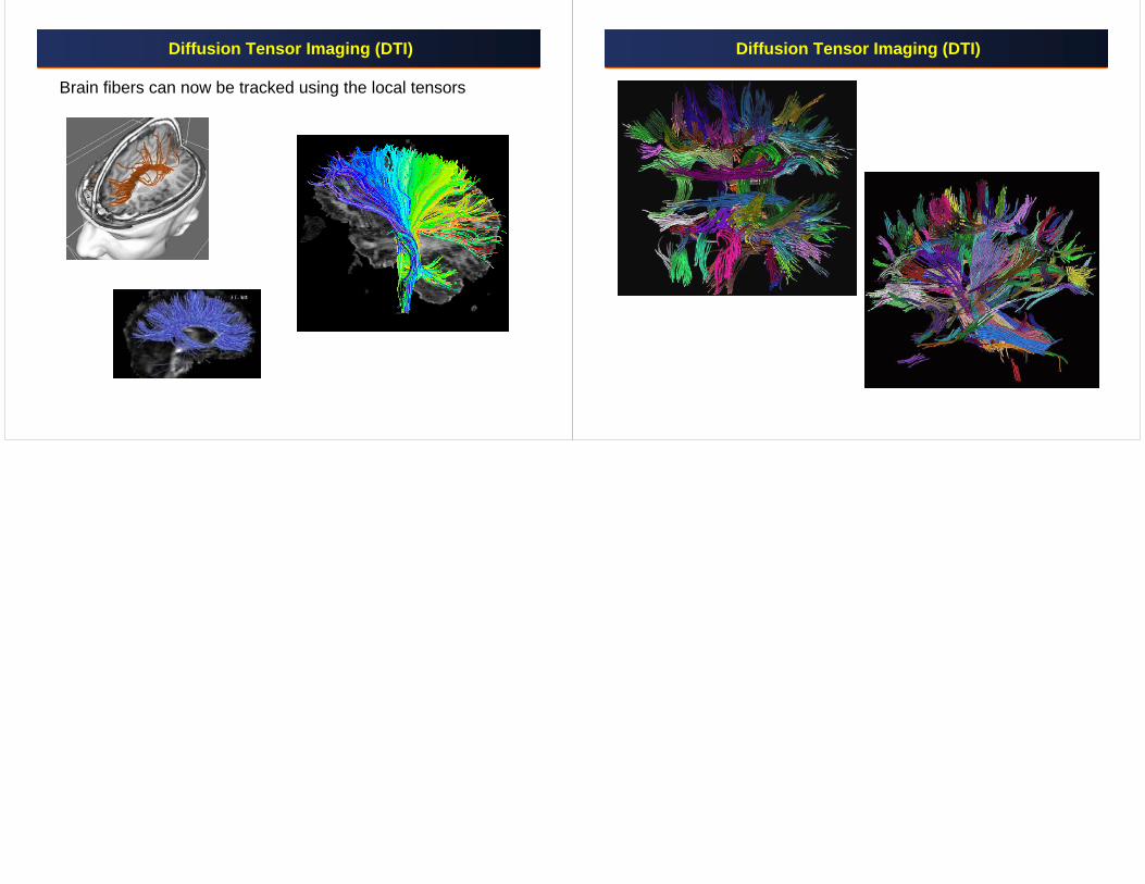
Diffusion Tensor Imaging (DTI)
Brain fibers can now be tracked using the local tensors
Diffusion Tensor Imaging (DTI)