1

Wolfram Burgard, Cyrill Stachniss, Maren

Bennewitz, Giorgio Grisetti, Kai Arras

Bayes Filter – Kalman Filter

Introduction to Mobile Robotics

2

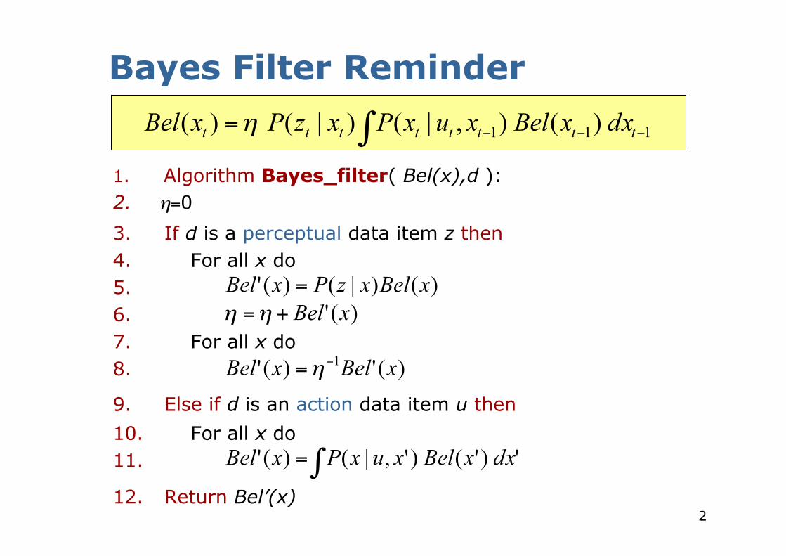
Bayes Filter Reminder

1.  Algorithm Bayes_filter( Bel(x),d ): 2.  η=0

3.  If d is a perceptual data item z then 4.  For all x do 5.  6.  7.  For all x do 8. 

9.  Else if d is an action data item u then

10.  For all x do 11. 

12.  Return Bel’(x)

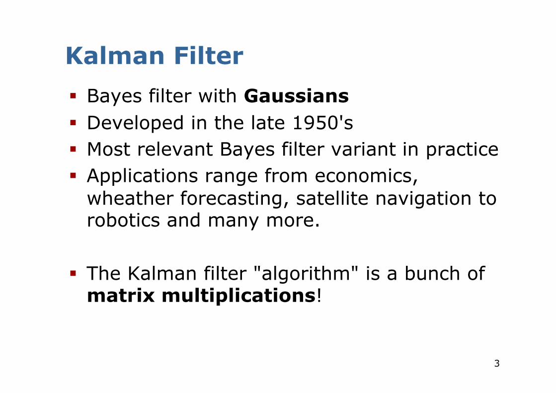
Kalman Filter

  Bayes filter with Gaussians   Developed in the late 1950's   Most relevant Bayes filter variant in practice   Applications range from economics,

wheather forecasting, satellite navigation to robotics and many more.

  The Kalman filter "algorithm" is a bunch of matrix multiplications!

3

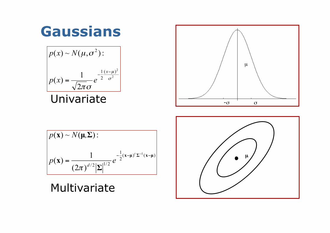
Gaussians

-σ σ

µ

Univariate

µ

Multivariate

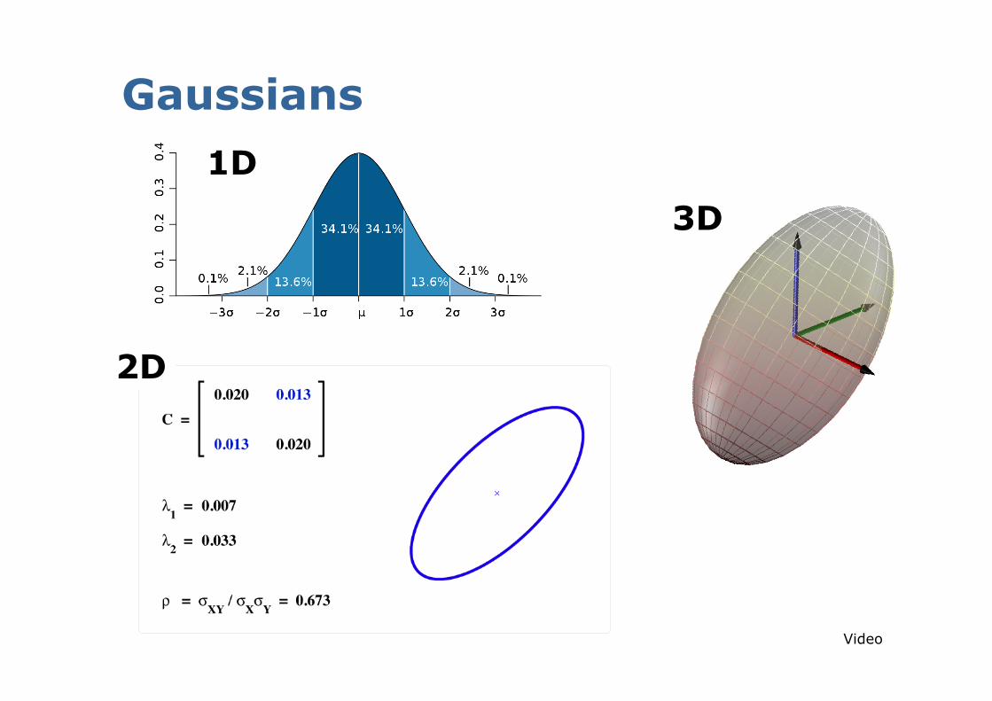
Gaussians

1D

2D

3D

Video

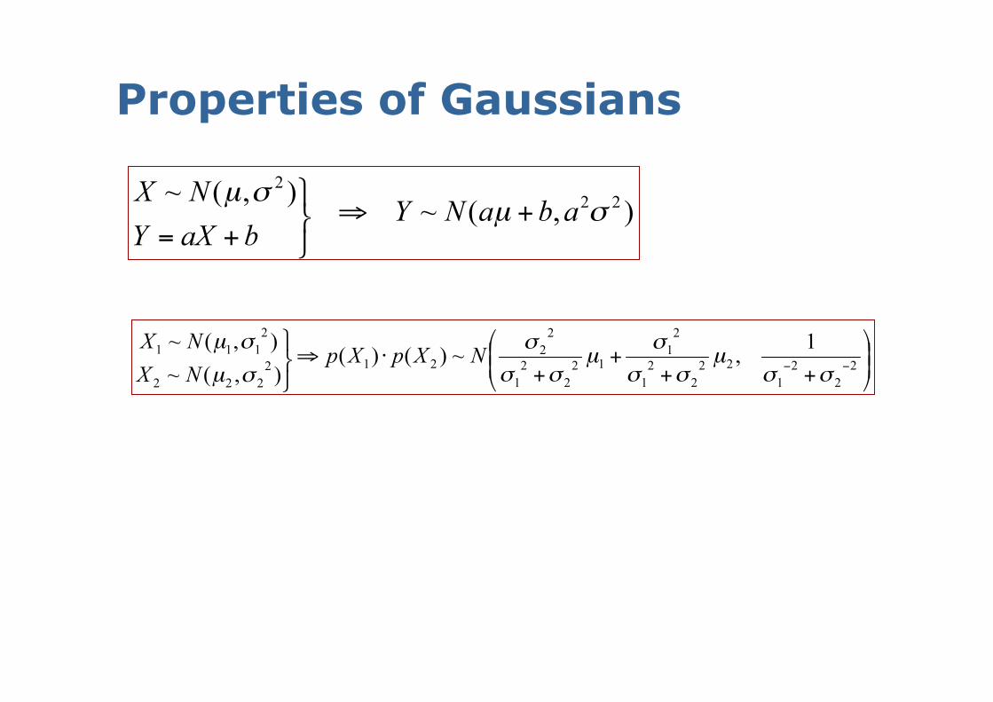
Properties of Gaussians

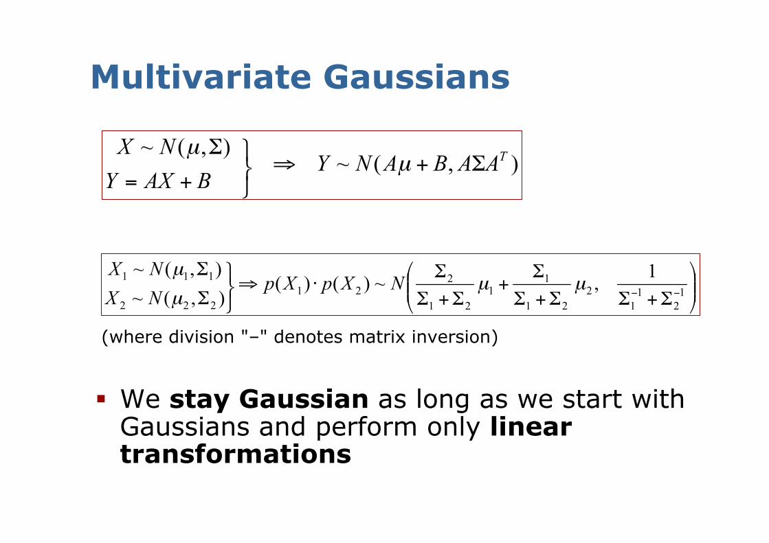
(where division "–" denotes matrix inversion)

  We stay Gaussian as long as we start with Gaussians and perform only linear transformations

Multivariate Gaussians

8

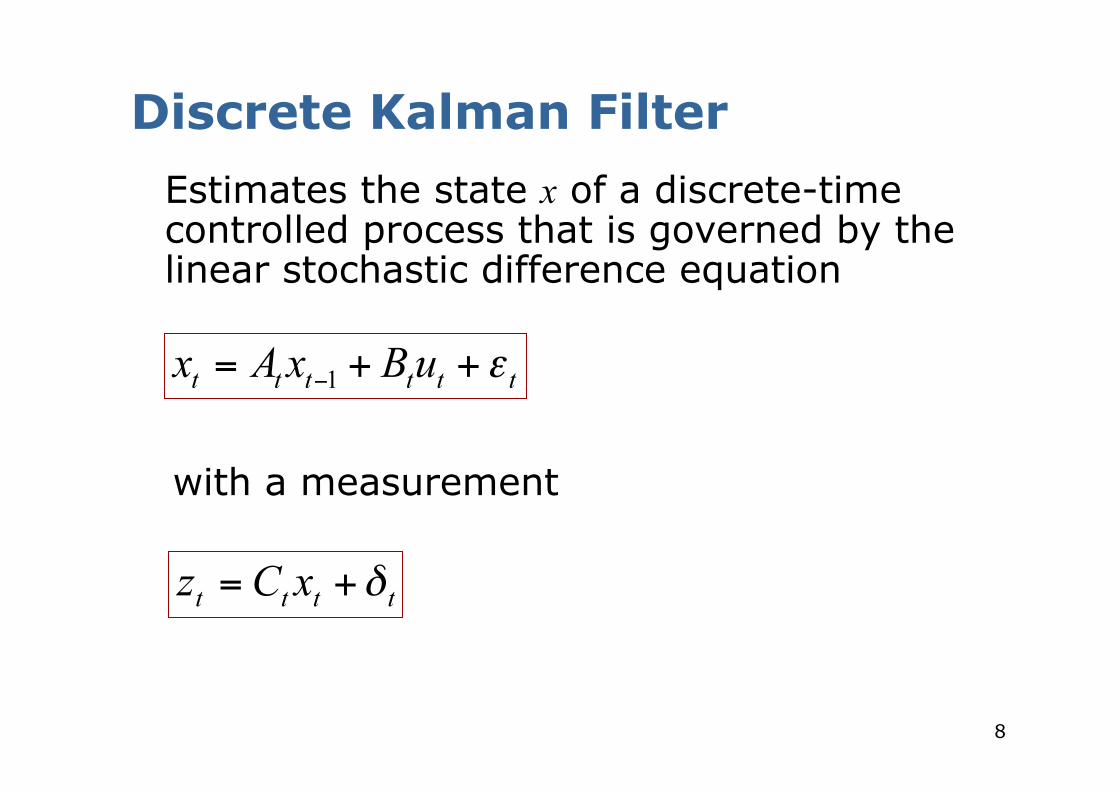
Discrete Kalman Filter

Estimates the state x of a discrete-time controlled process that is governed by the linear stochastic difference equation

with a measurement

9

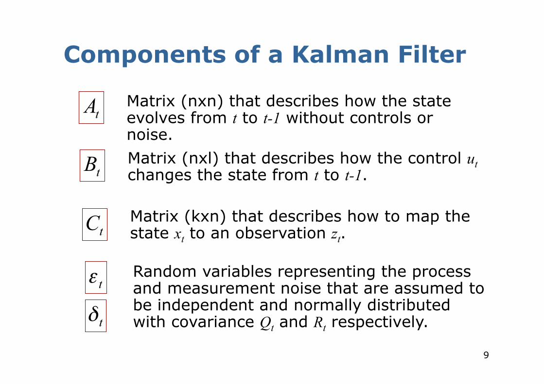
Components of a Kalman Filter

Matrix (nxn) that describes how the state evolves from t to t-1 without controls or noise.

Matrix (nxl) that describes how the control ut changes the state from t to t-1.

Matrix (kxn) that describes how to map the state xt to an observation zt.

Random variables representing the process and measurement noise that are assumed to be independent and normally distributed with covariance Qt and Rt respectively.

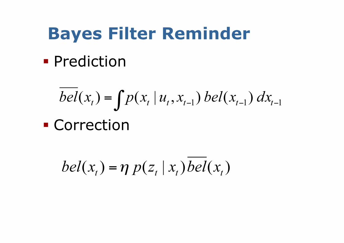
 Prediction

 Correction

Bayes Filter Reminder

11

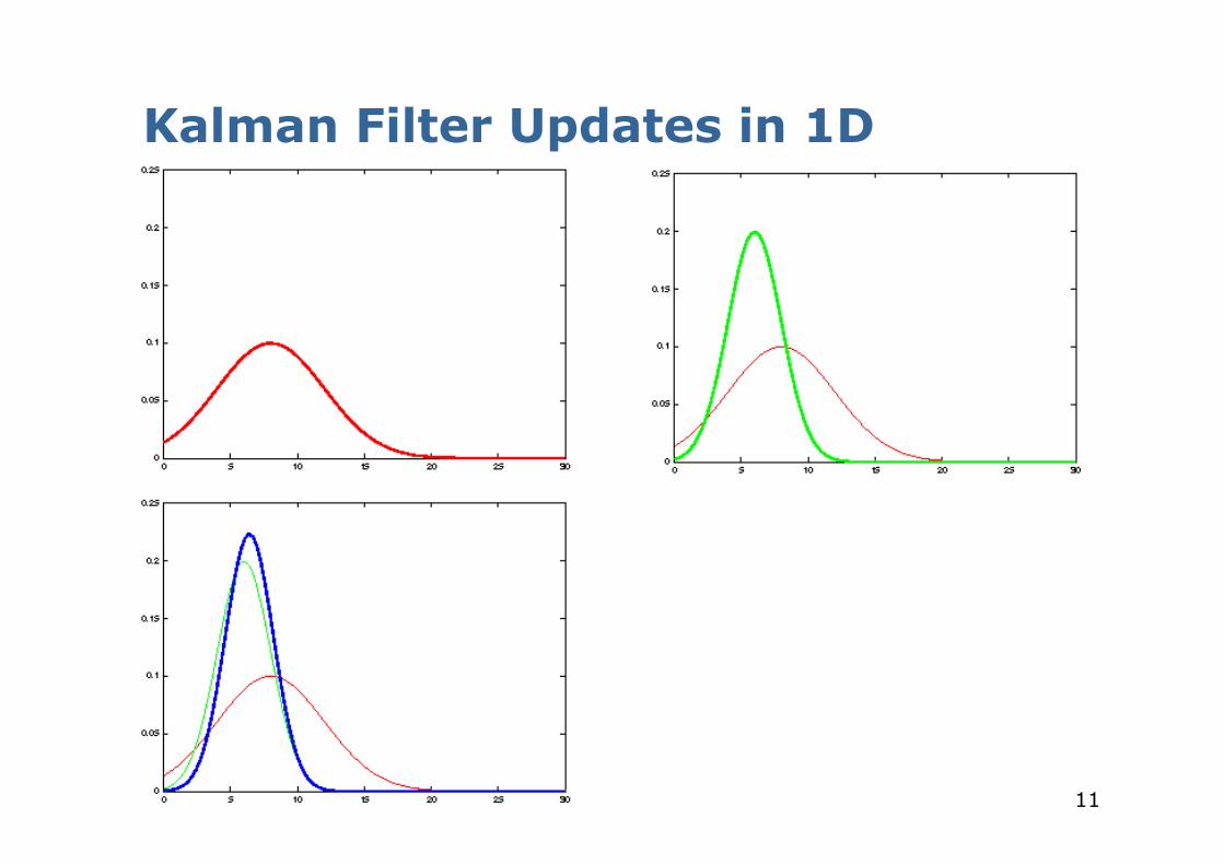
Kalman Filter Updates in 1D

12

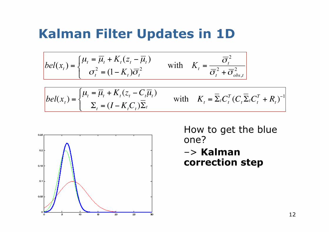
Kalman Filter Updates in 1D

€

bel(xt ) =µt = µ t + Kt (zt −Ctµ t )Σt = (I −KtCt )Σt

with Kt = ΣtCtT (CtΣtCt

T + Rt )−1

How to get the blue one? –> Kalman correction step

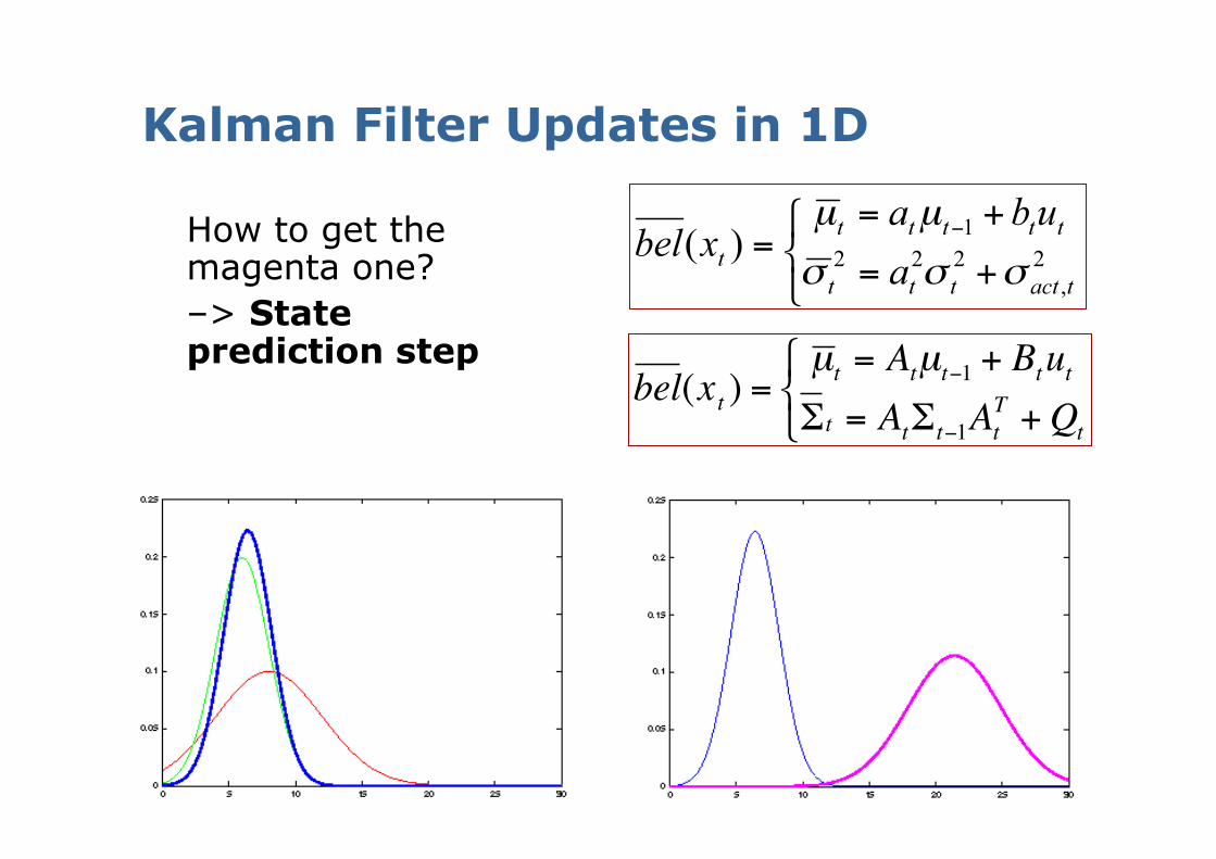
Kalman Filter Updates in 1D

€

bel(xt ) =µ t = Atµt−1 + BtutΣt = AtΣt−1At

T +Qt

How to get the magenta one? –> State prediction step

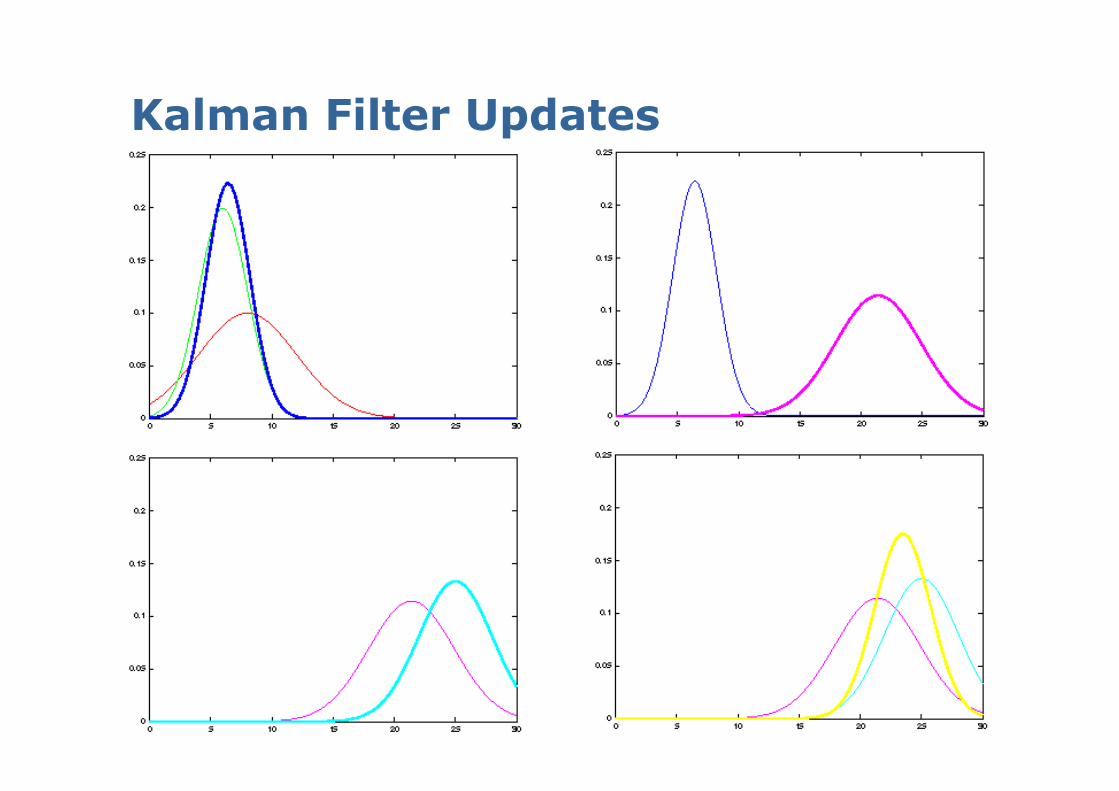
Kalman Filter Updates

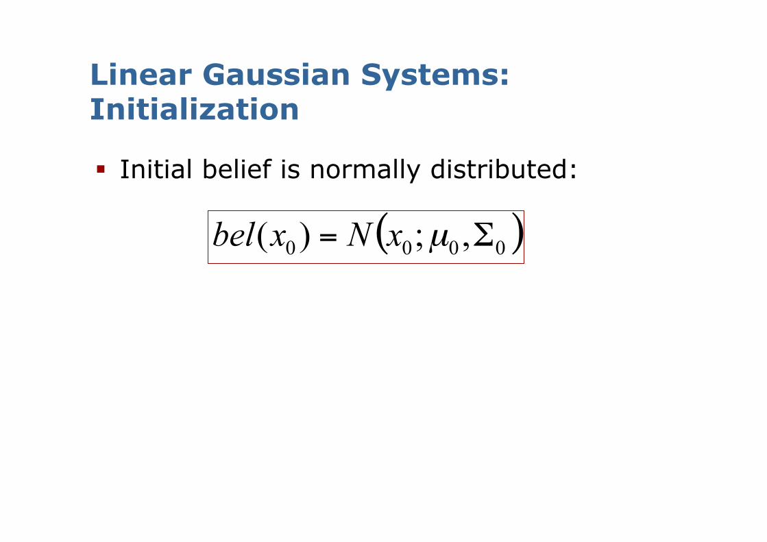
Linear Gaussian Systems: Initialization

  Initial belief is normally distributed:

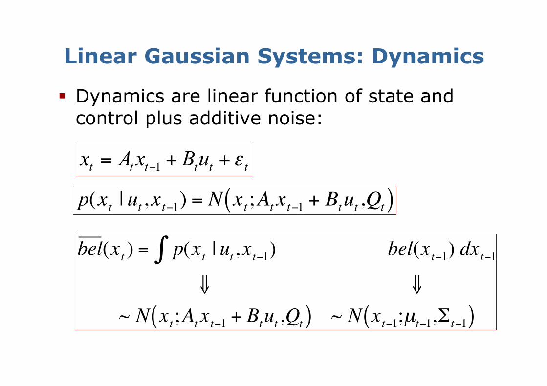
  Dynamics are linear function of state and control plus additive noise:

Linear Gaussian Systems: Dynamics

€

p(xt | ut ,xt−1) = N xt;At xt−1 + Btut ,Qt( )

€

bel(xt ) = p(xt | ut ,xt−1)∫ bel(xt−1) dxt−1⇓ ⇓

~ N xt;At xt−1 + Btut ,Qt( ) ~ N xt−1;µt−1,Σt−1( )

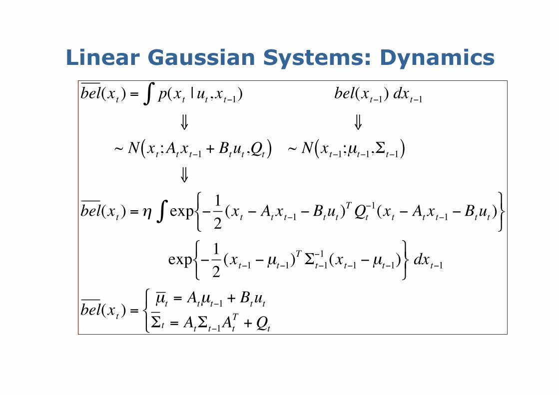
Linear Gaussian Systems: Dynamics

€

bel(xt ) = p(xt | ut ,xt−1)∫ bel(xt−1) dxt−1⇓ ⇓

~ N xt;At xt−1 + Btut ,Qt( ) ~ N xt−1;µt−1,Σt−1( )⇓

bel(xt ) =η exp −12(xt − At xt−1 − Btut )

T Qt−1(xt − At xt−1 − Btut )

∫

exp −12(xt−1 −µt−1)

T Σt−1−1 (xt−1 −µt−1)

dxt−1

bel(xt ) =µ t = Atµt−1 + BtutΣt = AtΣt−1At

T +Qt

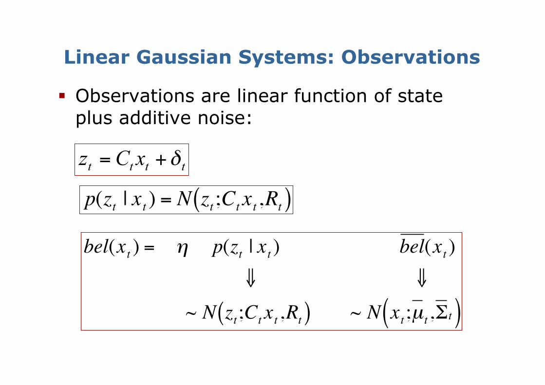
  Observations are linear function of state plus additive noise:

Linear Gaussian Systems: Observations

€

p(zt | xt ) = N zt ;Ct xt ,Rt( )

€

bel(xt ) = η p(zt | xt ) bel(xt )⇓ ⇓

~ N zt;Ct xt ,Rt( ) ~ N xt ;µ t ,Σt( )

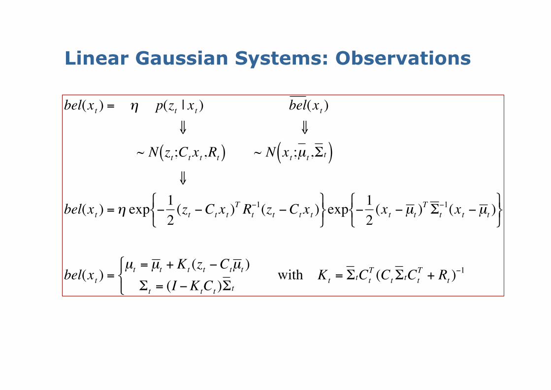
Linear Gaussian Systems: Observations

€

bel(xt ) = η p(zt | xt ) bel(xt )⇓ ⇓

~ N zt;Ct xt ,Rt( ) ~ N xt ;µ t ,Σt( )⇓

bel(xt ) =η exp −12

(zt −Ct xt )T Rt

−1(zt −Ct xt )

exp −12

(xt −µ t )T Σ t

−1(xt −µ t )

bel(xt ) =µt = µ t + Kt (zt −Ctµ t )Σt = (I −KtCt )Σt

with Kt = ΣtCtT (CtΣtCt

T + Rt )−1

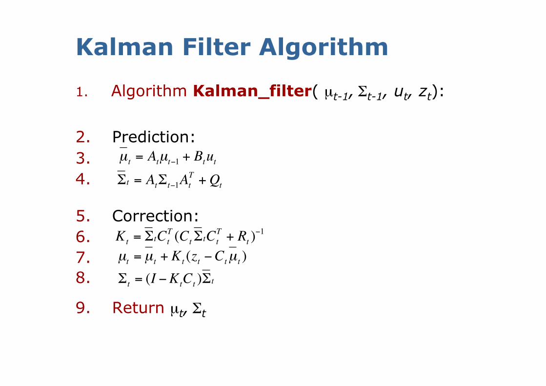
Kalman Filter Algorithm

1.  Algorithm Kalman_filter( µt-1, Σt-1, ut, zt):

2.  Prediction: 3.  4. 

5.  Correction: 6.  7.  8. 

9.  Return µt, Σt

€

µ t = Atµt−1 + Btut

€

Σt = AtΣt−1AtT +Qt

€

Kt = ΣtCtT (CtΣtCt

T + Rt )−1

€

µt = µ t + Kt (zt −Ctµ t )

€

Σt = (I −KtCt )Σt

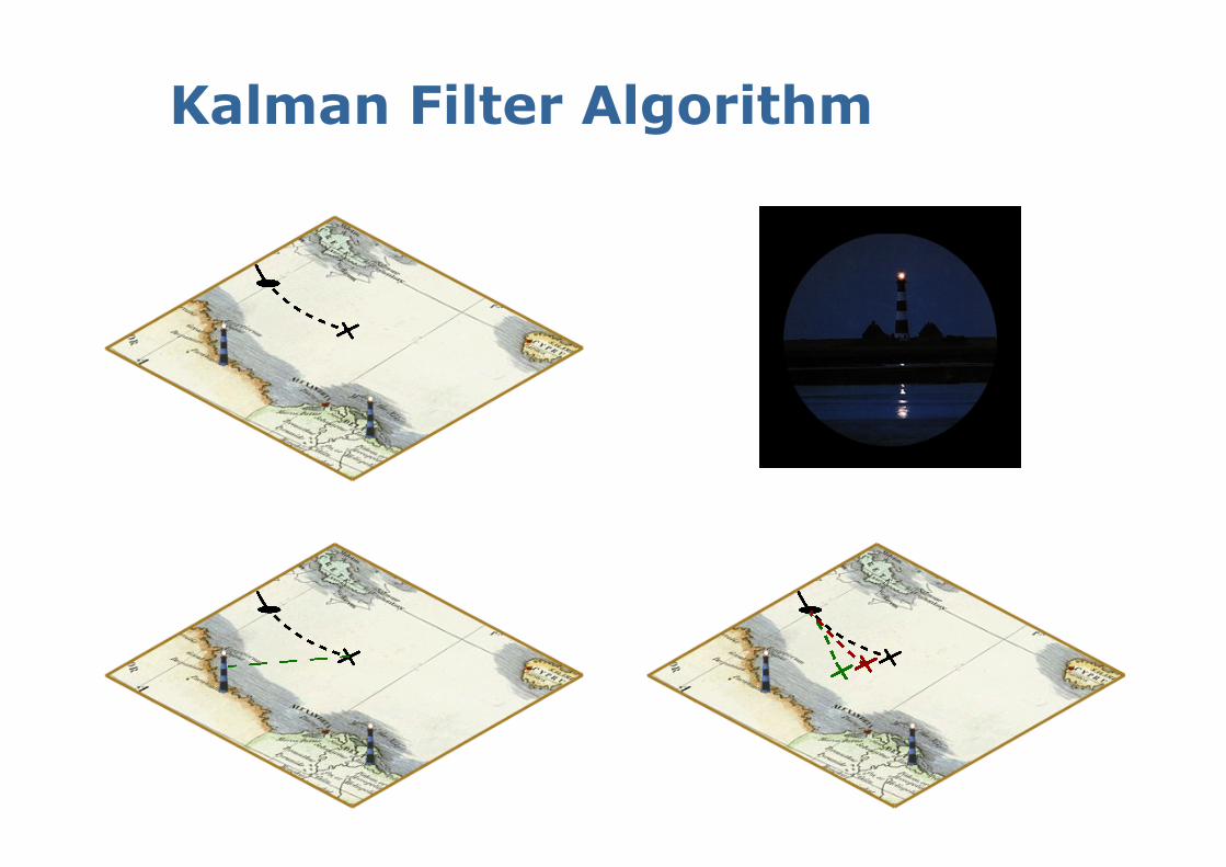
Kalman Filter Algorithm

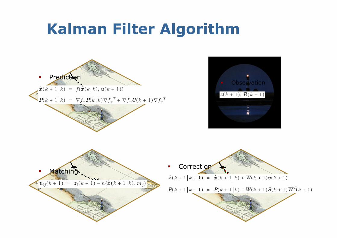
Kalman Filter Algorithm

  Prediction   Observation

  Matching   Correction

23

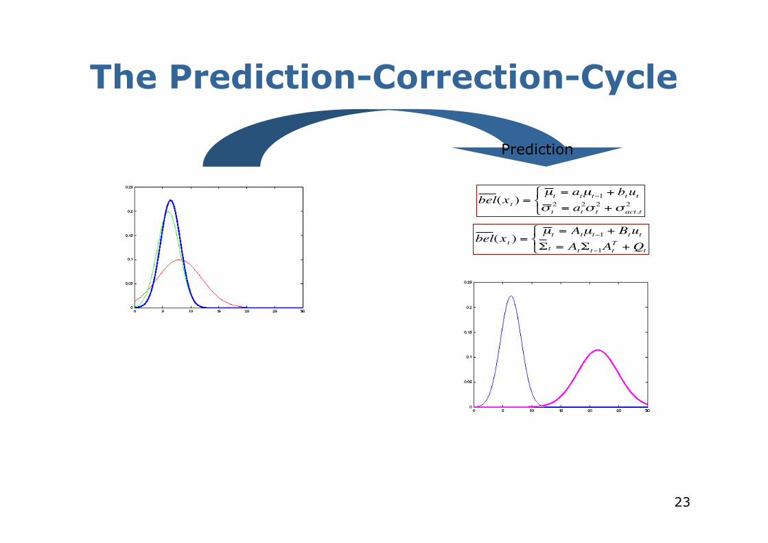
The Prediction-Correction-Cycle

€

bel(xt ) =µ t = Atµt−1 + BtutΣt = AtΣt−1At

T +Qt

€

bel(xt ) =µ t = atµt−1 + btutσ t2 = at

2σ t2 +σ act,t

2

Prediction

24

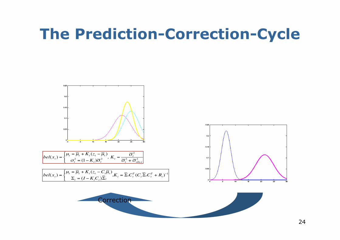
The Prediction-Correction-Cycle

€

bel(xt ) =µt = µ t + Kt (zt −Ctµ t )Σt = (I −KtCt )Σt

,Kt = ΣtCtT (CtΣtCt

T + Rt )−1

€

bel(xt ) =µt = µ t + Kt (zt −µ t )σ t

2 = (1−Kt )σ t2

, Kt =σ t

2

σ t2 +σ obs,t

2

Correction

25

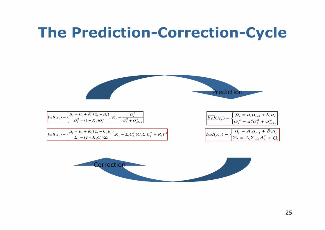
The Prediction-Correction-Cycle

€

bel(xt ) =µt = µ t + Kt (zt −Ctµ t )Σt = (I −KtCt )Σt

,Kt = ΣtCtT (CtΣtCt

T + Rt )−1

€

bel(xt ) =µt = µ t + Kt (zt −µ t )σ t

2 = (1−Kt )σ t2

, Kt =σ t

2

σ t2 +σ obs,t

2

€

bel(xt ) =µ t = Atµt−1 + BtutΣt = AtΣt−1At

T +Qt

€

bel(xt ) =µ t = atµt−1 + btutσ t2 = at

2σ t2 +σ act,t

2

Correction

Prediction

Kalman Filter Summary

  Highly efficient: Polynomial in the measurement dimensionality k and state dimensionality n:

O(k2.376 + n2)

  Optimal for linear Gaussian systems!

  Most robotics systems are nonlinear!

Nonlinear Dynamic Systems

  Most realistic robotic problems involve nonlinear functions

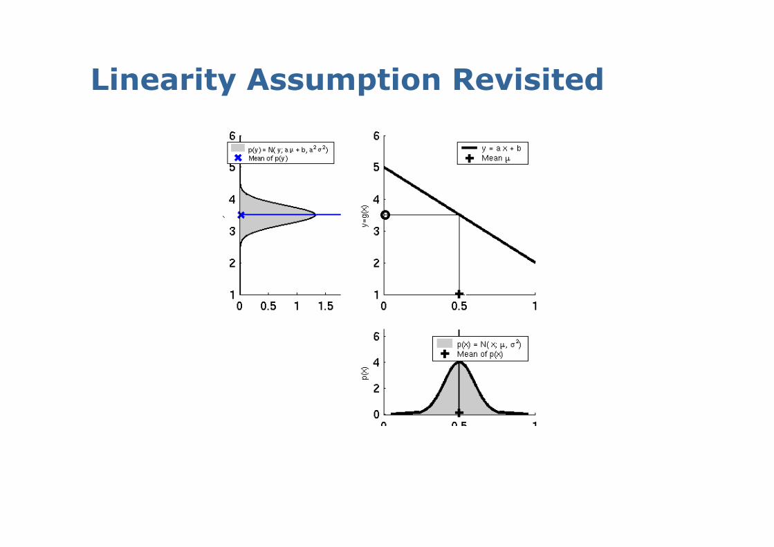
Linearity Assumption Revisited

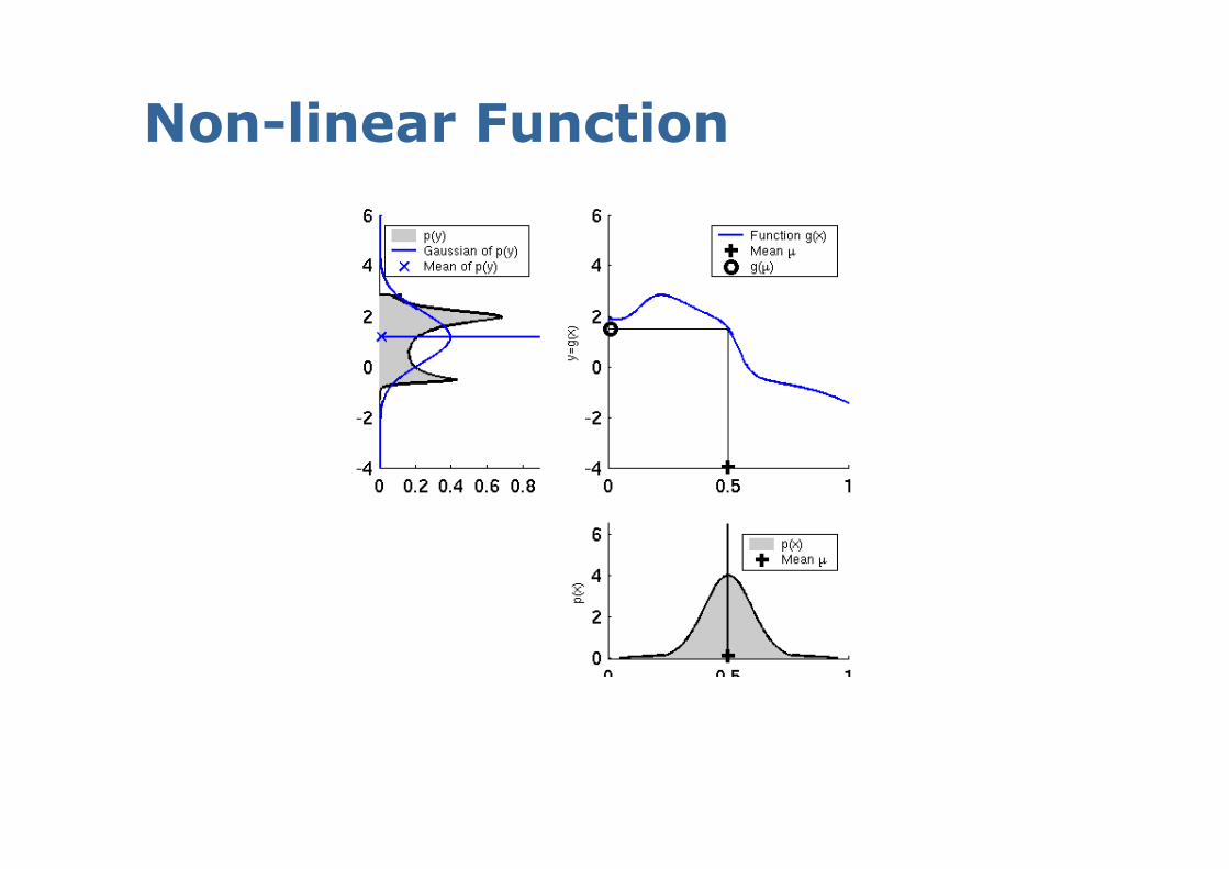
Non-linear Function

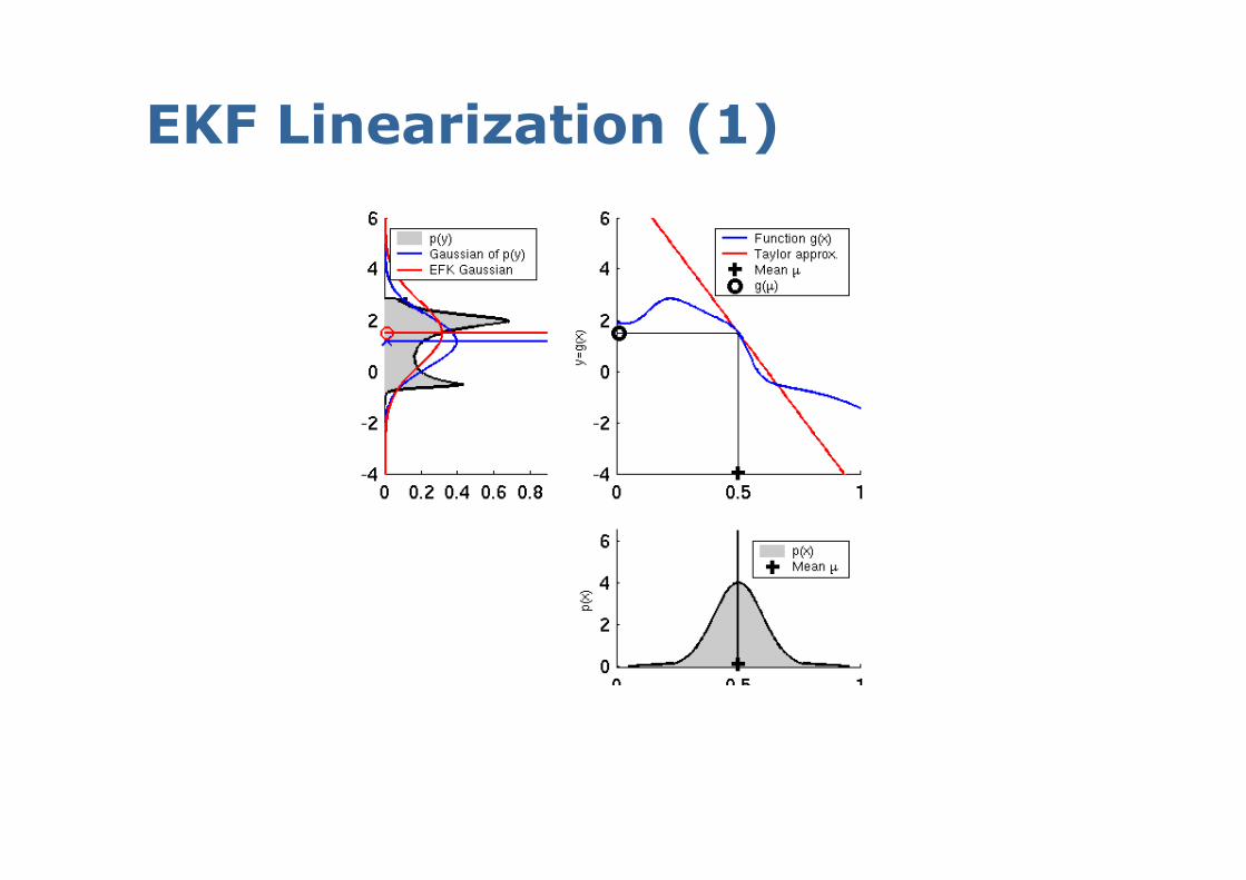
EKF Linearization (1)

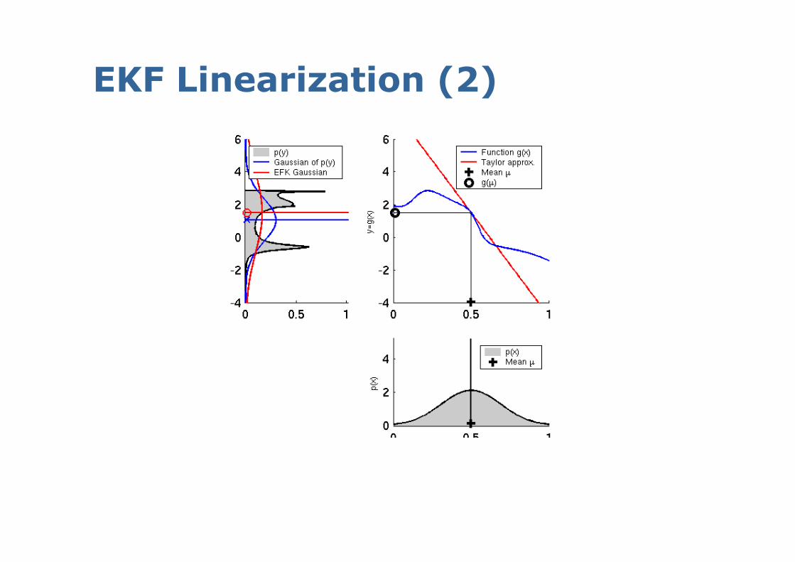
EKF Linearization (2)

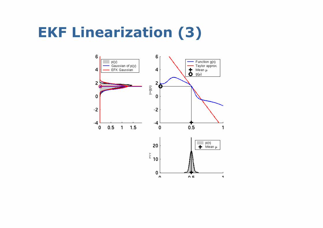
EKF Linearization (3)

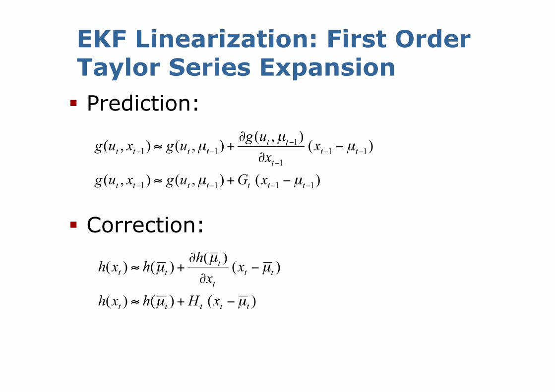
  Prediction:

  Correction:

EKF Linearization: First Order Taylor Series Expansion

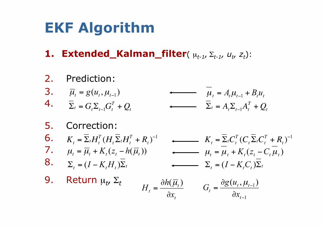
EKF Algorithm

1.   Extended_Kalman_filter( µt-1, Σt-1, ut, zt):

2.  Prediction: 3.  4. 

5.  Correction: 6.  7.  8. 

9.  Return µt, Σt

€

Σt =GtΣt−1GtT +Qt

€

Kt = ΣtHtT (HtΣtHt

T + Rt )−1

€

Σt = AtΣt−1AtT +Qt

€

Kt = ΣtCtT (CtΣtCt

T + Rt )−1