Embed Size (px)
Citation preview
Introduction to Quantum Field Theory
Arthur JaffeHarvard University
Cambridge, MA 02138, USAc©by Arthur Jaffe. Reproduction only with permission of the author.
24 May, 2005 at 7:26

ii
Contents
I Life of a Single Particle 1
1 Introduction 3
2 Life of a Particle in Real Time 52.1 Quantum Theory . . . . . . . . . . . . . . . . . . . . . . . . . . . . . . . . . . . . . 52.2 Poincare Symmetry . . . . . . . . . . . . . . . . . . . . . . . . . . . . . . . . . . . . 62.3 Stability . . . . . . . . . . . . . . . . . . . . . . . . . . . . . . . . . . . . . . . . . . 82.4 Special Features of a Single Particle . . . . . . . . . . . . . . . . . . . . . . . . . . . 82.5 The Configuration Space Representation . . . . . . . . . . . . . . . . . . . . . . . . 8
2.5.1 The Momentum and Energy Operators . . . . . . . . . . . . . . . . . . . . . 92.6 The Momentum Space Representation . . . . . . . . . . . . . . . . . . . . . . . . . 112.7 The Lorentz-Invariant Scalar Product . . . . . . . . . . . . . . . . . . . . . . . . . . 122.8 The Poincare Group on H . . . . . . . . . . . . . . . . . . . . . . . . . . . . . . . . 13
3 Life of a Particle at Imaginary Time 153.1 Wave Functions . . . . . . . . . . . . . . . . . . . . . . . . . . . . . . . . . . . . . 183.2 The Euclidean Laplacian and its Green’s Function . . . . . . . . . . . . . . . . . . 183.3 Reflection Positivity . . . . . . . . . . . . . . . . . . . . . . . . . . . . . . . . . . . 203.4 Osterwalder-Schrader Quantization . . . . . . . . . . . . . . . . . . . . . . . . . . . 22
3.4.1 The Sobolev Space H−1(O) . . . . . . . . . . . . . . . . . . . . . . . . . . . 233.4.2 Why “Quantization”? . . . . . . . . . . . . . . . . . . . . . . . . . . . . . . 243.4.3 Quantization of Operators . . . . . . . . . . . . . . . . . . . . . . . . . . . . 243.4.4 Some Examples of Quantized Operators . . . . . . . . . . . . . . . . . . . . 263.4.5 Unbounded Operators on H1 . . . . . . . . . . . . . . . . . . . . . . . . . . 283.4.6 Quantization Domains . . . . . . . . . . . . . . . . . . . . . . . . . . . . . . 293.4.7 Quantization of Space-Time Rotations . . . . . . . . . . . . . . . . . . . . . 30
3.5 Poincare Symmetry from Euclidean Symmetry . . . . . . . . . . . . . . . . . . . . . 303.6 Properties of Matrices and Operators . . . . . . . . . . . . . . . . . . . . . . . . . . 30
3.6.1 Operator Monotonicity . . . . . . . . . . . . . . . . . . . . . . . . . . . . . . 313.6.2 Two Monotonicity Preserving Functions . . . . . . . . . . . . . . . . . . . . 323.6.3 The Perron-Frobenius Theorem . . . . . . . . . . . . . . . . . . . . . . . . . 34
iii
iv CONTENTS
3.7 Reflection Positivity Revisited . . . . . . . . . . . . . . . . . . . . . . . . . . . . . . 35
3.7.1 Mirror Charges and Classical Green’s Functions . . . . . . . . . . . . . . . . 35
3.7.2 Reflection Positivity & Operator Monotonicity . . . . . . . . . . . . . . . . . 37
3.7.3 Reflection Invariance Ensures Monotonicity . . . . . . . . . . . . . . . . . . 38
3.7.4 Monotonicity & Reflection Positivity . . . . . . . . . . . . . . . . . . . . . . 40
3.8 Space-Time Compactification . . . . . . . . . . . . . . . . . . . . . . . . . . . . . . 40
3.8.1 Periodic Green’s Function . . . . . . . . . . . . . . . . . . . . . . . . . . . . 41
3.8.2 Periodic Time Reflection . . . . . . . . . . . . . . . . . . . . . . . . . . . . . 42
3.8.3 Reflection Positivity on Td . . . . . . . . . . . . . . . . . . . . . . . . . . . . 44
3.8.4 Quantization on Td and the Role of S = ΘS . . . . . . . . . . . . . . . . . . 46
3.9 Mirror Space-Time Lattice . . . . . . . . . . . . . . . . . . . . . . . . . . . . . . . . 49
3.9.1 Green’s Functions . . . . . . . . . . . . . . . . . . . . . . . . . . . . . . . . . 49
3.9.2 Time Reflection . . . . . . . . . . . . . . . . . . . . . . . . . . . . . . . . . . 49
3.9.3 Reflection Positivity . . . . . . . . . . . . . . . . . . . . . . . . . . . . . . . 49
II Fock Space 51
4 Sums and Products 55
4.1 The Direct Sum . . . . . . . . . . . . . . . . . . . . . . . . . . . . . . . . . . . . . . 55
4.2 The Tensor Product . . . . . . . . . . . . . . . . . . . . . . . . . . . . . . . . . . . 56
4.2.1 Definition of K1 ⊗K2 . . . . . . . . . . . . . . . . . . . . . . . . . . . . . . . 56
4.2.2 Tensor Products of Operators . . . . . . . . . . . . . . . . . . . . . . . . . . 58
4.2.3 The Pointwise Operator Product . . . . . . . . . . . . . . . . . . . . . . . . 60
4.2.4 Pointwise Products Preserve Positivity . . . . . . . . . . . . . . . . . . . . . 61
4.3 n-Fold Tensor Products . . . . . . . . . . . . . . . . . . . . . . . . . . . . . . . . . . 61
4.4 Tensor Powers . . . . . . . . . . . . . . . . . . . . . . . . . . . . . . . . . . . . . . 63
4.4.1 The Map Γ . . . . . . . . . . . . . . . . . . . . . . . . . . . . . . . . . . . . 64
4.5 Symmetric Powers . . . . . . . . . . . . . . . . . . . . . . . . . . . . . . . . . . . . 64
4.5.1 Bosonic Fock Space . . . . . . . . . . . . . . . . . . . . . . . . . . . . . . . 67
4.5.2 Bosonic Creation and Annihilation Operators . . . . . . . . . . . . . . . . . 68
4.6 Anti-Symmetric Powers . . . . . . . . . . . . . . . . . . . . . . . . . . . . . . . . . 69
4.7 Fermionic Fock Space . . . . . . . . . . . . . . . . . . . . . . . . . . . . . . . . . . 70
4.7.1 Fermionic Creation and Annihilation Operators . . . . . . . . . . . . . . . . 71
5 Number Bounds 73
5.1 Estimates on m(f) . . . . . . . . . . . . . . . . . . . . . . . . . . . . . . . . . . . . 73
5.2 Nice Vectors . . . . . . . . . . . . . . . . . . . . . . . . . . . . . . . . . . . . . . . . 75
5.3 The Weyl Algebra . . . . . . . . . . . . . . . . . . . . . . . . . . . . . . . . . . . . . 75
5.4 Some Additional Properties when H = H−1/2(Rd−1) . . . . . . . . . . . . . . . . . . 77
CONTENTS v
III Quantum Fields 79
6 The Free Bosonic Field 836.1 The Local Field . . . . . . . . . . . . . . . . . . . . . . . . . . . . . . . . . . . . . . 83
6.1.1 The Hilbert Space . . . . . . . . . . . . . . . . . . . . . . . . . . . . . . . . 836.1.2 Time-Zero Fields . . . . . . . . . . . . . . . . . . . . . . . . . . . . . . . . . 85
6.2 The Free Field . . . . . . . . . . . . . . . . . . . . . . . . . . . . . . . . . . . . . . . 866.2.1 Fields at a Point . . . . . . . . . . . . . . . . . . . . . . . . . . . . . . . . . 876.2.2 Momentum Space Representation . . . . . . . . . . . . . . . . . . . . . . . . 876.2.3 Commutation Relation . . . . . . . . . . . . . . . . . . . . . . . . . . . . . . 88
6.3 Imaginary Time Fields . . . . . . . . . . . . . . . . . . . . . . . . . . . . . . . . . . 896.4 Compact Space . . . . . . . . . . . . . . . . . . . . . . . . . . . . . . . . . . . . . . 896.5 Forms and Number Bounds . . . . . . . . . . . . . . . . . . . . . . . . . . . . . . . 896.6 Poincare Invariance . . . . . . . . . . . . . . . . . . . . . . . . . . . . . . . . . . . . 896.7 Locality . . . . . . . . . . . . . . . . . . . . . . . . . . . . . . . . . . . . . . . . . . 896.8 Wightman Functions . . . . . . . . . . . . . . . . . . . . . . . . . . . . . . . . . . . 896.9 Reeh-Schlieder Property . . . . . . . . . . . . . . . . . . . . . . . . . . . . . . . . . 89
7 The Fundamental Bound for Fields 917.1 The Fundamental Bound . . . . . . . . . . . . . . . . . . . . . . . . . . . . . . . . . 92
7.1.1 The Fundamental Bound and Field Operators . . . . . . . . . . . . . . . . . 937.1.2 The Fundamental Bound and Expectation Values . . . . . . . . . . . . . . . 103
IV Euclidean Fields 105
V Some Analytic Tools 109
8 Linear Transformations on Hilbert Space 1118.1 Hilbert Space . . . . . . . . . . . . . . . . . . . . . . . . . . . . . . . . . . . . . . . 1118.2 Operators . . . . . . . . . . . . . . . . . . . . . . . . . . . . . . . . . . . . . . . . . 1128.3 Self-Adjoint Operators . . . . . . . . . . . . . . . . . . . . . . . . . . . . . . . . . . 117
8.3.1 Analytic Vectors . . . . . . . . . . . . . . . . . . . . . . . . . . . . . . . . . 1178.4 Operators between Different Hilbert Spaces . . . . . . . . . . . . . . . . . . . . . . . 1188.5 Forms . . . . . . . . . . . . . . . . . . . . . . . . . . . . . . . . . . . . . . . . . . . 119
8.5.1 The Graph of T . . . . . . . . . . . . . . . . . . . . . . . . . . . . . . . . . . 1208.6 Trace . . . . . . . . . . . . . . . . . . . . . . . . . . . . . . . . . . . . . . . . . . . . 1208.7 Convergence of Operators . . . . . . . . . . . . . . . . . . . . . . . . . . . . . . . . 121
8.7.1 Convergence Based on Traces . . . . . . . . . . . . . . . . . . . . . . . . . . 1218.7.2 Uniform Convergence . . . . . . . . . . . . . . . . . . . . . . . . . . . . . . . 1228.7.3 Strong Convergence . . . . . . . . . . . . . . . . . . . . . . . . . . . . . . . . 123

vi CONTENTS
8.7.4 Weak Convergence . . . . . . . . . . . . . . . . . . . . . . . . . . . . . . . . 1248.7.5 Graph Convergence . . . . . . . . . . . . . . . . . . . . . . . . . . . . . . . . 124
9 Fourier Transformation 1259.1 Fourier Transforms on L2 . . . . . . . . . . . . . . . . . . . . . . . . . . . . . . . . . 1259.2 Schwartz Space . . . . . . . . . . . . . . . . . . . . . . . . . . . . . . . . . . . . . . 131

Part I
Life of a Single Particle
1

Chapter 1
Introduction
Our goal is to present a brief and self-contained introduction to quantum field theory from theconstructive point of view. We try to motivate some basic results and relate them to interestingopen problems.
One should mention right at the start that one still does not understand whether quantummechanics and special relativity are compatible at a fundamental level in our Minkowski four-spaceworld. One generally assumes that this means finding a complete Yang-Mills gauge theory or theinteraction of gauge fields with fermionic matter fields, the simplest form being quantum chromo-dynamics (QCD). Associated with this picture is the belief that the fundamental vector mesonexcitations are massive (as opposed to photons, which arise in the limiting case of an abelian gaugesymmetry. The proof of the existence of a “mass gap” appears a necessary integral part of solvingthe entire puzzle.
This question remains one of the deepest open issues in theoretical physics, as well as in math-ematics. Basically the question remains: can one give a mathematical foundation to the theory offields in four-dimensions? In other words, can do quantum mechanics and special relativity lie onthe same footing as the classical physics of Newton, Maxwell, Einstein, or Schrodinger—all of whichfits into a mathematical framework that we describe as the language of physics. This glaring gapin our fundamental knowledge even dwarfs questions of whether there are other more complicatedand sophisticated approaches to physics—those that incorporate gravity, strings, or branes—forunderstanding their fundamental significance lies far in the future. In fact, one believes that stringyproposals, if they can be fully implemented, have limiting cases that appear as relativistic quan-tum fields, just as relativistic quantum fields describe non-relativistic quantum theory and classicalphysics in various limiting cases.
We begin with the quantum mechanical treatment of a particle of a given mass. If we assumethat the symmetry of the quantum theory includes the transformations of special relativity, thenmuch of the structure follows naturally. We then develop the basic Euclidean point of view, thatarises from attempting to analytically continue Lorentz symmetry to Euclidean symmetry. Thisprovides also the natural connection with path integrals. We specialize the case of a single, free,bosonic particle; this illustrates many of the main ideas.
3
4 CHAPTER 1. INTRODUCTION
Each method gives a route to quantization. In the path integral framework we encounter classicalfields defined on Euclidean space (with a positive metric and Euclidean symmetry). One encountersa condition known as reflection (or Osterwalder-Schrader) positivity that allows one obtain a quan-tum theory (on Hilbert space) from a path integral. The quantum theory that one finds agrees withthe usual picture of canonical quantization that one learns in standard field theory. The quantumtheory also comes with a representation of the inhomogeneous Lorentz group (the Poincare group)that arises from an analytic continuation of the quantization of the Euclidean group.
Thus the two fundamental points of view mesh to one. We first investigate a special casethat relates to the Gaussian path integral and the free quantum field. We then give the generalconstruction that applies for bosonic non-linear fields.
Introduction to Quantum Field Theory 24 May, 2005 at 7:26
Chapter 2
Life of a Particle in Real Time
We introduce quantum theory for a single, spinless particle of mass m > 0. We assume that theparticle moves in Euclidean space with coordinates ~x and of dimension s = d − 1. The usual caseis s = 3, but for until we encounter interactions we also allow for arbitrary integer values of s.
2.1 Quantum Theory
The quantum state of a particle is described by a wave function f. We deal concretely with someconcepts that appear in more abstract form in later chapters. A particle follows the usual rules ofquantum theory:
• The wave function of a quantum system is a vector f in a Hilbert space H, comprising possiblewave functions.
• Quantum mechanical observables (such as the energy H or the momentum ~P ) are self-adjointlinear transformations on H.
• The value of an observable T in the state f is its expectation 〈f, T f〉H.
• A group G of physical symmetries is described by a unitary representation U(G) of G on H.
• The self-adjoint generator of a one-parameter subgroup of symmetries G is identified with aspecific physical observable.
There are two alternative ways in which one views the action of a symmetry group G.
HP. In the Heisenberg picture, one considers that the symmetry acts on the observables. So anobservable T transforms under a symmetry element g ∈ G as
T → T g = U(g)TU(g)∗ . (2.1)
The value of the transformed observable in the state f is given by the expectation
〈f, T g f〉H = 〈f, U(g)TU(g)∗ f〉H . (2.2)
5
6 CHAPTER 2. LIFE OF A PARTICLE IN REAL TIME
SP. Alternatively, in the Schrodinger picture, one considers that the symmetry acts on thestates. In this case the state vector f transforms under the symmetry according to the anti-representation
f → fg = U(g)∗f , (2.3)
for which U(g1)∗U(g2)
∗ = U(g2g1)∗. The value of the observable T in the transformed state
fg also equals (2.2).
The one-parameter group of time-translations defines the dynamics of quantum theory, and thisgroup has a special significance in quantum theory. The time-translation group U(t) = eitH isgenerated by the energy observable H (also called the Hamiltonian). Its action in the Schrodingerpicture is
f → f t = U(t)∗f = e−itHf , (2.4)
and this gives the solution to the Schrodinger equation.
i~∂f t
∂t= Hf t , with initial data f 0 = f , (2.5)
in units where Planck’s constant ~ = 1. Therefore one often calls e−itH the Schrodinger group.
2.2 Poincare Symmetry
We are concerned here with quantum theory that is compatible with special relativity. So we expectthat the symmetry group of relativity has a unitary representation on H. This group of symmetriesis sometimes called the Poincare group. An element of the Poincare group Λ, a comprises both aLorentz transformation Λ and a translation a of Minkowski space, which we now define.
The coordinates of d-dimensional Minkowski space-time Md are x = (~x, t). The met-ric g in Minkowski space is a d × d diagonal matrix with entries gµν , and with eigenvalues−1,−1,−1, . . . ,−1, 1. The Minkowski square of x is1
x2M =
∑µν
xµgµνxν = t2 − ~x2 . (2.6)
Time-like vectors have positive squares, space-like vectors have negative squares, and light-likevectors have square zero.
Lorentz transformations act linearly as x → Λx, and they are specified by real d × d matricesΛ, chosen to preserve the Minkowski square of x. Thus the Lorentz matrices satisfy
ΛTgΛ = g , (2.7)
1For simplicity of notation we generally will suppress the subscript M in denoting the square of the Minkowskilength. In this chapter all squares or inner products of Minkowski-space vectors will be assumed to be Minkowskiscalar products. On the other hand, inner products of spatial components ~x of vectors will be assumed to haveEuclidean (positive) signature.
Introduction to Quantum Field Theory 24 May, 2005 at 7:26
2.2. POINCARE SYMMETRY 7
where ΛT denotes the transpose of the matrix Λ. This condition is equivalent to the preservationof the Minkowski squared length. For one can write in matrix notation x2 = xTgx, so
(Λx)2 = xT ΛTgΛx = xTgx = x2 . (2.8)
Translations in the Poincare group act in an affine manner, x→ x+a. One defines the Poincaretransformation Λ, a to act as
Λ, ax = Λx+ a . (2.9)
The multiplication law for the Poincare group (2.9) is
Λ1, a1Λ2, a2 = Λ1Λ2,Λ1a2 + a1 , (2.10)
and in particular,
Λ, a = I, aΛ, 0 . (2.11)
The inverse Λ, a−1 = Λ−1,−Λ−1a acts on Minkowski space as
Λ, a−1 x = Λ−1(x− a) . (2.12)
In the case Λ = I, this multiplication law ensures that all space-time translations commute, for
U(I, a1)U(I, a2) = U(I, a2 + a1) = U(I, a2)U(I, a1) . (2.13)
The basic physical assumption of relativistic quantum theory is that one can identify the self-adjoint generators of the one-parameter subgroups of the Poincare group with the following physicalobservables.
• One identifies the d generators of the space-time translations U(I, a) with the components of
the momentum vector ~P and the energy H,
U(I, a) = eiadH−i~a·~P = eia·P , (2.14)
where P = (~P ,H) denotes the momentum-energy vector.
• Likewise one identifies the (d−1)(d−2)/2 infinitesimal generators Lij of rotations in the planesxi xj as angular momentum. One identifies the (d− 1) self-adjoint generators Mi generatinghyperbolic rotations in the planes xi xd as Lorentz boosts.
The commutativity of the space-time translation subgroup means that the components Pµ of themomentum-energy vector are mutually commuting operators,
[Pµ, Pν ] = 0 , for all 1 ≤ µ, ν ≤ d . (2.15)
Introduction to Quantum Field Theory 24 May, 2005 at 7:26
8 CHAPTER 2. LIFE OF A PARTICLE IN REAL TIME
2.3 Stability
In quantum theory, one also generally assumes that there is a state of lowest energy—the vacuumstate. Without this assumption the world would be unstable and under a perturbation it couldcollapse. Thus a fundamental assumption of quantum theory is that one can add a constant to theHamiltonian to make it positive. One generally writes,
0 ≤ H , (2.16)
although in certain circumstances the absolute zero of energy can play a role.
2.4 Special Features of a Single Particle
Furthermore in special relativity, a particle of mass m satisfies the energy-momentum relation,
P 2 = H2 − ~P 2 = m2 . (2.17)
Equivalently, if we can write
H =(~P 2 +m2
)1/2, (2.18)
so this H must be defined as the positive square root. Also m2 ≥ 0, so we can define the massoperator M as the positive square root of P 2,
M =(P 2)1/2
=(H2 − ~P 2
)1/2. (2.19)
The mass operator commutes with the entire representation U(Λ, a),
U(Λ, a)M = MU(Λ, a) . (2.20)
The spectrum of the mass operator M labels the hyperboloids in the spectrum of the representationU(Λ, a), and the group maps each hyperboloid into itself. If H is the space of quantum-mechanicalstates for a single particle of mass m, then we require that every vector in H be an eigenvector ofthe mass operator M with eigenvalue m,
M f = m f . (2.21)
2.5 The Configuration Space Representation
One obtains further structure by assuming a particular representation of the wave functions f asfunctions f(~x) on configuration space ~x ∈ Rs. Here s = d− 1 denotes that we take an s-dimensionaltime slice of Md. According to the picture above, the symmetries of quantum theory (includingPoincare space-time symmetry) act on the Hilbert space of functions f defined on a time slice.
Introduction to Quantum Field Theory 24 May, 2005 at 7:26
2.5. THE CONFIGURATION SPACE REPRESENTATION 9
According to the description of symmetries in (2.4), the group G acts on state vectors in theSchrodinger picture according to an anti-representation. If a symmetry g ∈ G acts on Rs by
~x→ g~x , (2.22)
then the natural anti-representation is
(U(g)∗f) (~x) = f(g~x) , (2.23)
for which(U(g1)
∗U(g2)∗f) (~x) = (U(g2)
∗f) (g1~x) = f(g2g1~x) = (U(g2g1)∗f) (~x) . (2.24)
In case G is also measure-preserving in H, then U(g) defined in this way is also unitary.
2.5.1 The Momentum and Energy Operators
Consider the spatial translation subgroup T~a = I, (~a, 0) of the Poincare group, which acts on Rs
byT~a~x = ~x+ ~a . (2.25)
Then(U(T~a)
∗f) (~x) = f(~x+ ~a) . (2.26)
But according to the rules of quantum theory, the group U(T~a) is the same as the subgroup e−i~a·~P
in (2.14) generated by the momentum. Therefore,
(U(T~a)∗f) (~x) =
(ei~a·~P f
)(~x) = f(~x+ ~a) . (2.27)
Therefore one infers that the momentum operator ~P in configuration space has the usual represen-tation in quantum theory for wave functions defined on configuration-space,
~P = −i~∇x , (2.28)
where ~∇x denotes the gradient. We conclude further that in this representation, the one-particleHamiltonian H defined in (2.18) has the form
H =(−~∇2
x +m2)1/2
. (2.29)
Thus the solution to the Schrodinger equation
f t(~x) =(e−itHf
)(~x) , with f 0 = f , (2.30)
introduced in (2.5), also satisfies the second-order wave equation called the Klein-Gordon equation.Denoting the wave operator by
=∂2
∂t2−∇2 , (2.31)
Introduction to Quantum Field Theory 24 May, 2005 at 7:26
10 CHAPTER 2. LIFE OF A PARTICLE IN REAL TIME
the Klein-Gordon equation for mass m is the equation( +m2
)f t(~x) = 0 . (2.32)
Note that as the square root of a differential operator, this one-particle Hamiltonian operatorH is non-local. The solution (2.30) to the Klein-Gordon equation spreads instantaneously over allall of space, Rs. This fact can be illustrated by the (non-normalizable) configuration-space waveinitial value f = δ for the equation, which illustrates the basic point. One can compute the solution
f t(~x) =(e−itHf
)(~x) , with f 0(~x) = δ(~x) , (2.33)
in closed form. For example in case s = 3 and |~x| = r > t ≥ 0, one finds
f t(~x) =i
2π2r
∫ ∞
mζe−ζr sinh
(t√ζ2 −m2
)dζ , (2.34)
which is nonzero.
Exercise 2.5.1. Solutions to the Klein-Gordon wave equation propagate with finite speed. But f t(~x)instantly spreads from its localization at the origin (at t = 0) to all space (for any t > 0), as fors = 3 in (2.34). Does this fact not contradict the laws of special relativity that influence cannotpropagate faster than the speed of light?
There is an interesting scalar product defined on solutions to the Schrodinger equation, or onpositive energy solutions to the Klein-Gordon equation of the form (2.30). Consider
〈f, 2Hg〉L2(Rs) = i
⟨f t,∂
∂tg t
⟩L2(Rs)
−⟨∂
∂tf t, g t
⟩L2(Rs)
. (2.35)
As a consequence of the Schrodinger equation, the right side of (2.35) equals 〈f t, 2Hg t〉L2(Rs). Fur-thermore the same equation shows that the this expression does not depend on t, as its timederivative is
∂
∂t
⟨f t, 2Hg t
⟩L2(Rs)
= i
⟨f t,∂2
∂t2g t
⟩L2(Rs)
−⟨∂2
∂t2f t, g t
⟩L2(Rs)
= −i
(⟨f t, H2g t
⟩L2(Rs)
−⟨H2f t, g t
⟩L2(Rs)
)= 0 . (2.36)
In the final step, we use the fact that H is self adjoint on L2(Rs). Thus one can evaluate〈f t, 2Hg t〉L2(Rs) at t = 0, and as m ≤ H, one infers that the expectation 〈f, 2Hf〉L2(Rs) definesan inner product on solutions of the Schrodinger equation. (Note that the right side of (2.35) isnegative when f t = g t is a negative-energy solution to the Klein-Gordon equation.)
Introduction to Quantum Field Theory 24 May, 2005 at 7:26
2.6. THE MOMENTUM SPACE REPRESENTATION 11
2.6 The Momentum Space Representation
The momentum representation is defined by the Fourier transformation of the configuration spacerepresentation. It has the feature that the momentum operator ~P acts as multiplication by acoordinate ~p. Define the Fourier transform as
(Ff) (~p) =1
(2π)s/2
∫Rs
f(~x)e−i~p~xd~x . (2.37)
Sometimes it is less cumbersome to write2
f(p) = (Ff) (p) . (2.38)
Clearly Fourier transformation F is a linear transformation, for if the Fourier transform of f and g
exist, then both F(f + g) = Ff + Fg, and Fλf = λFf for any λ ∈ C.We also claim that F is a unitary transformation on the Hilbert space L2(Rs), namely every
L2(Rs) function has a Fourier transform and
FF∗ = F∗F = I . (2.39)
The outline of the argument is that Plancherel’s formula states that F preserves L2(Rs) innerproducts, ⟨
f, g⟩
L2(Rs)= 〈f, g〉L2(Rs) , for all f, g ∈ L2(Rs) . (2.40)
Furthermore the Fourier inversion theorem says that F is invertible, and hence it is unitary. Actuallythe simplest way to show that F is unitary on L2 is to exhibit an orthogonal basis of eigenfunctionsfor F.3 The forumla for the inverse of F is the Fourier inversion formula
f(~x) =1
(2π)s/2
∫Rs
f(~p)ei~p~xd~p , (2.41)
and an expression of its validity for all square-integrable functions.The Fourier representation is called the momentum representation. In fact this is natural because
we saw in (2.28) that the quantum-mechanical momentum operator ~P the form ~P = −i~∇x. Thus
in the Fourier representation the momentum operator ~P acts as multiplication by the coordinate ~p.In particular,
~P f(~x) = −i∇xf(~x) =1
(2π)s/2
∫Rs~p f(~p)ei~p~xd~p . (2.42)
2One must be careful with this notation in our context. One must guard against confusing f with our f, that weintroduce in a later chapter to denote something very different—the quantization of f.
3In fact, the Gaussian function Ω0 = π−s/4 exp(−~x2/2
)is an eigenvector of F with eigenvalue 1. The Hermite
functions, given by products of polynomials in each coordinate times Ω0 complete an orthogonal basis of eigenfunc-tions, and each has an eigenvalue of either ±1 or ±i. Thus the proof that F is unitary is equivalent to the proof thatthe Hermite functions are a basis for L2. See Appendix Appendix ??, for a complete proof.
Introduction to Quantum Field Theory 24 May, 2005 at 7:26
12 CHAPTER 2. LIFE OF A PARTICLE IN REAL TIME
Write the self adjoint operators for each component of the momentum are multiplication by thecoordinate of ~p, or simply ~P = ~p. In other words, for all f ∈ H,
~P f(~p) = ~p f(~p) . (2.43)
Likewise, the Hamiltonian H acts in the momentum space representation as the operator H ofmultiplication by the function ω(~p), defined as the positive square root
H = ω(~p) =(~p2 +m2
)1/2. (2.44)
Hence (e−itHf
)(~x) =
1
(2π)s/2
∫Rse−itω(~p) f(~p)ei~p~xd~p , (2.45)
or (e−itH f
)(~p) = e−itω(~p) f(~p) . (2.46)
2.7 The Lorentz-Invariant Scalar Product
One can now arrive easily at the correct scalar product by considering the momentum representationof the wave functions f. The wave functions f(~p) only depend on the spatial components of themomenta ~p. Let us suppose that the Hilbert space norm can be defined by an integral over alld components of p. Then one obtains a Lorentz-invariant measure on the mass-m hyperboloidp2 = p2
d − ~p2 = m2 as follows: restrict the Lorentz-invariant Lebesgue measure dp = d~p dpd tothe mass-m hyperboloid by multiplying it with the Lorentz invariant Dirac measure δ(p2 − m2).Furthermore, one wants positive energies, so also restrict the integral to the positive-pd. Since thewave functions do not depend on pd, the pd integral can be done separately, namely∫
pd>0δ(p2 −m2)dpd =
∫pd>0
δ((pd − ω(~p))(pd + ω(~p))) dpd =1
2ω(~p). (2.47)
Thus we obtain a natural Lorentz-invariant scalar product by multiplying this density with f(~p) g(~p)and integrating over d~p. Let ⟨
f, g⟩H
=∫
Rd−1f(~p) g(~p)
d~p
2ω(~p). (2.48)
This defines a Hilbert space H of functions f(~p) such that
∫ ∣∣∣f(~p)∣∣∣2 d~p
2ω(~p)<∞ . (2.49)
The operator of multiplication by (2ω(~p))−1 in Fourier space can also be expressed in configura-tion space. It is given by the operator (2H)−1, with H the non-local (pseudo-differential) operator
Introduction to Quantum Field Theory 24 May, 2005 at 7:26
2.8. THE POINCARE GROUP ON H 13
(2.29). This is the special Hamiltonian for a single free particle of mass m, so we also denote theone-particle Hamiltonian H by
H = ω =(−~∇2
x +m2)1/2
. (2.50)
By relating both spaces to L2(Rd−1), one can write the configuration-space Hilbert space H in termsof the momentum representation H. In particular, regard F as a map from H to H, and F∗ as thebackwards map from H to H. Then define H with the inner product
〈f, g〉H =⟨f, g⟩H. (2.51)
Define the operator G = (2ω)−1 on L2(Rs) with integral kernel G(~x− ~y). It is given by
(Gf) (~x) =1
(2π)(d−1)/2
∫Rs
(2ω(~p))−1f(~p) ei~p·~x d~p =
∫RsG(~x− ~y)f(~y)d~y , (2.52)
where G(~x− ~y) is the generalized function
G(~x− ~y) =1
(2π)(d−1)/2
∫Rs
1
2ω(~p)ei~p·(~x−~y)d~p . (2.53)
The Hilbert space of generalized functions with the inner product (2.51) occurs frequently inanalysis and is known as the Sobolev space H = H−1/2(Rs). In summary,
〈f, g〉H = 〈f, g〉H−1/2(Rs) =⟨f, (2ω)−1
g⟩
L2(Rs)= 〈f, Gg〉L2(Rs) =
⟨f, g⟩H. (2.54)
One can also write the scalar product (2.35) on solutions to the Schrodinger equation in the form
〈f, g〉L2(Rs) = i(⟨
f t, ∂∂t
g t⟩H−⟨
∂∂t
f t, g t⟩H
). (2.55)
The index −1/2 on the Sobolev space H−1/2 means that the space includes not only all L2(Rs)functions, but also generalized functions which when acted on by ω−1/2 are square integrable.Functions in H are said to include all functions that are one-half a derivative of an L2(Rs) function.4
In Fourier space, the function ω(~p)−1/2 decays as |~p|−1/2 for large |~p|, so the corresponding Fouriertransforms when multiplied by an inverse half power of |~p| for large |~p| are square integrable.
2.8 The Poincare Group on HIt is now straightforward to write down the representation U(Λ, a) of the Poincare group. Let usstart by finding the representation U(Λ, a) on the Hilbert space H in the momentum representation.
4One can define similar spaces Hp(Rs) by replacing the transformation ω−1 in the inner product by the transfor-mation ω−2p. In the case of positive p, the Sobolev space does not include all square integrable functions, only thosein the domain of ωp as an operator on L2(Rs).
Introduction to Quantum Field Theory 24 May, 2005 at 7:26
14 CHAPTER 2. LIFE OF A PARTICLE IN REAL TIME
Although the wave function f(~p) depends on ~p ∈ Rd−1, it is convenient to regard it as a function ofa Minkowski-space momentum variable p with d components, that lies on the hyperboloid p2 = m2,and with pd > 0. There is a unique correspondence between (d − 1)-vectors ~p and such d-vectorsp = (~p, ω(~p)). Define f(p) by
f(p) = f(~p) . (2.56)
With this notation, it is clear that(U(I, a)∗f
)(p) = e−iadω(~p)+i~a·~p f(p) = e−ia·p f(p) . (2.57)
Since U(I, a) multiplies f(p) by a phase, it acts on H as a unitary transformation.Furthermore, the matrix Λ maps the mass-m hyperboloid into itself. So define the anti-
representation U(Λ, 0)∗ in a fashion similar to the rule (2.23), giving(U(Λ, 0)∗f
)(p) = f(Λp) . (2.58)
Then using the composition law U(Λ, a)∗ = U(Λ, 0)∗U(I, a)∗, we find(U(Λ, a)∗f
)(p) = e−ia·Λp f(Λp) . (2.59)
Proposition 2.8.1. The transformation (2.59) defines the adjiont of a unitary representationU(Λ, a) of the Poincare group on the one-particle momentum-space Hilbert space H. Under Fouriertransformation, it gives the unitary representation
U(Λ, a) = F∗U(Λ, a)F , (2.60)
on on the configuration-space Hilbert space H.
Proof. The transformation U(Λ, a)∗ satisfies the multiplication law for an anti=representation,as this is true of both U(I, a) and U(Λ, 0). Therefore we need only show that U(Λ, a)∗ is unitary.
We have already seen that U(I, a)∗ is unitary, so we only need to verify that U(Λ, 0)∗ is unitary.We see this by expressing the H inner product in invariant form,⟨
U(Λ, 0)∗f, U(Λ, 0)∗g⟩H
=∫
Rdf(Λp) g(Λp) δ(p2 −m2) dp
=∫
Rdf(p) g(p) δ(p2 −m2) dp =
⟨f, g⟩H. (2.61)
Therefore U(Λ, 0)∗ is a unitary anti-representation on H, and U(Λ, a) is a unitary representation.The statement about the representation on H follows from the fact that F∗F = I on H and
FF∗ = I on H. That F∗U(Λ, a)F is a representation then follows from the fact that U(Λ, a) is arepresentation. In order to show that the representation is unitary, it is sufficient to prove that itpreserves scalar products. The fundamental relation (2.51) shows that
〈U(Λ, a)f, U(Λ, a)g〉H =⟨U(Λ, a)Ff, U(Λ, a)Fg
⟩H
=⟨U(Λ, a)f, U(Λ, a)g
⟩H
=⟨f, g⟩H
= 〈f, g〉H .
(2.62)Thus U(Λ, a) = F∗U(Λ, a)F is unitary, and the proof is complete.
Introduction to Quantum Field Theory 24 May, 2005 at 7:26
Chapter 3
Life of a Particle at Imaginary Time
In Chapter 2 we described such a particle by a quantum-mechanical wave function f(~x), with ~x ∈Rd−1. These wave functions were chosen to lie in the one-particle Hilbert space H = H−1/2(Rd−1),namely the Sobolev space H−1/2 that contains all square integrable functions as well as vectorswhich have finite norm in the inner product
〈f, g〉H = 〈f, g〉H−1/2(Rd−1) =⟨f, (2ω)−1g
⟩L2(Rd−1)
, (3.1)
with ω = (−∇2 + m2)1/2 equal to the one-particle Hamiltonian. By using this description, ratherthan the usual L2 wave functions, we have an easy way to describe quantum theory in a Lorentzcovariant fashion, and we found a representation of the Poincare group on H.
In this chapter we give a different perspective on the ordinary quantum theory of a singlespinless, positive msss-m particle on Rd−1. Here we switch to Euclidian space-time Rd, where spaceand time enjoy the same geometry—although we still distinguish a special time direction in orderto make a connection with ordinary quantum theory. Space-time points are vectors
x = (~x, xd) ∈ Rd , with Euclidean length squared x2 = ~x2 + x2d . (3.2)
The last coordinate xd, which is the imaginary time. It corresponds in many cases to the analyticcontinuation from Minkowski space to purely imaginary times, xd = it.
Euclidean wave functions will be functions f(x) on Euclidean space-time, that are elements ofthe Euclidean Hilbert space E . We choose E so the inner product is naturally invariant under allrotations and translations (Euclidean transformations) of Rd. A straight-forward choice for thespace of wave functions might be L2(Rd), with the inner product
〈f, g〉L2(Rd) =∫
Rdf(x) g(x) dx . (3.3)
However, this is not the space we use. Just as in the quantum theory of Chapter 2, the space ofLebesgue square-integrable functions is not the natural choice for the Euclidean Hilbert space.
15
16 CHAPTER 3. LIFE OF A PARTICLE AT IMAGINARY TIME
Rather, we choose for E the somewhat larger Sobolev space E = H−1(Rd). Elements of thisspace are generalized functions with inner product equal to
〈f, g〉E = 〈f, g〉H−1(Rd) =⟨f, (−∆ +m2)−1g
⟩L2(Rd)
, (3.4)
where ∆ =∑d
j=1 ∂2/∂x2
j is the Laplacian on Rd.Life in Euclidean space is different from life in Minkowski space, at least for non-zero time. So
before considering that issue, let us mention how one can identify the Euclidean picture with theMinkowski picture on the time-zero hyperplane.
A very nice property of the Euclidean wave functions that we have chosen is that they havea localization to a sharp time, and this is one reason for the choice E = H−1(Rd). In fact, thisspace includes sharp-time wave functions that have the spatial dependence f(~x) ∈ H, namely theone-particle wave functions introduced in Chapter 2. At time zero, these special wave functionshave the form
f(~x, t) = f(~x) δ(t) . (3.5)
We suppress the variables and write such a product wave-function f as f = f⊗ δ.1
These functions are vectors in the Hilbert space E , namely
(f⊗ δ) ∈ H−1(Rd) , if f ∈ H−1/2(Rd−1) . (3.6)
The inner product between two such special wave-functions localized at time zero is
〈f⊗ δ, g⊗ δ〉E = 〈f, g〉H . (3.7)
This gives the real justification for our choice. It can be interpreted as a way to identify certainEuclidean wave functions in E = H−1(Rd) that behave exactly as the ordinary one-particle wavefunctions H = H−1/2(Rd−1). These special Euclidean wave-functions are a subspace of E . We havechosen the normalization of the inner product so that we obtain the elementary relation (3.7) forthis imbedding.
There are many other nice consequences of this relationship between E and H that one can seeby going away from xd = 0 to the Euclidean point (~x, xd). This corresponds to a Minkowski point(~x, it) that is analytically continued to imaginary time,
(~x, xd) ↔ (~x, it) . (3.8)
In order to illustrate this point, let us consider another elementary example. Consider the timetranslation transformation Ts(~x, xd) → (~x, xd − s). This transformation acts on L2(Rd) ∈ E as aunitary group. It is defined on smooth functions g(x) ∈ L2(Rd) by
(Tsg) (~x, xd) = g(~x, xd − s) . (3.9)
1We do not explain the notation ⊗ for “tensor product” here, but return at length to this topic in Chapter 4.
Introduction to Quantum Field Theory 24 May, 2005 at 7:26
17
The Laplacian ∆ commutes with time translations, so Ts also acts as a unitary transformation onE = H−1(Rd),
T ∗s Ts = Ts T∗s = I . (3.10)
Denote the translated delta function by δs(t) = δ(t− s), so one can write
Ts (g⊗ δ) = g⊗ δs . (3.11)
As Ts is unitary, one could carry out the calculation (3.7) at any time s; there is nothing specialabout time zero. Hence one finds that for any s ∈ R,
〈f⊗ δs, g⊗ δs〉E = 〈f, g〉H . (3.12)
We conclude that the scalar product of sharp time vectors can only depend on the difference in thetime of their localizations.
If we consider two different times, the matrix elements of Ts give the interesting relation thatgeneralizes (3.7). In §3.4 we show that for s ≥ 0,
〈(f⊗ δ) , Ts (g⊗ δ)〉E = 〈f⊗ δ, g⊗ δs〉E=
⟨f, e−sωg
⟩H. (3.13)
Here ω is the single-particle energy operator introduced earlier. Furthermore, the inner product inE is invariant under time-reflection, so (3.13) is unchanged if we replace s by −s, so
〈(f⊗ δ) , Ts (g⊗ δ)〉E =⟨f, e−|s|ωg
⟩H. (3.14)
Observe that on the left one has the matrix elements of a unitary operator Ts acting on E . Onthe right side, one obtains the corresponding matrix elements on H of the operator
R(s) = e−|s|ω , (3.15)
which is the self adjoint contraction that one obtains by analytically continuing the Schrodingergroup e−isω to purely imaginary time s in the upper or lower complex half-plane, depending onwhether the time is positive or negative. On the other hand, the operator Ts itself does not havean analytic continuation to complex s. But the equalities (3.13)–(3.14) show that certain matrixelements of Ts do have analytic continuations.
More generally, each unitary unitary Euclidean transformation (Rd-rotation or space-time trans-lation) acting on E corresponds in a 1-1 fashion with the analytic continuation of a unitary rep-resentation of the Poincare transformations (Lorentz transformations and space-time translations)acting on the space H.
In order to assure the analytic continuation of matrix elements of the Euclidean transformationson E , one must restrict consideration to a subspace of E . The functions that one studies belong tothe subspace of “positive time functions,” namely those what vanish for negative times, or H−1(Rd
+),where the subscript designates the positive time half space.
A more general correspondence between the spaces H and E arises from considering time re-flection between positive-time and negative-time functions, and using the property of reflectionpositivity, explained in §3.3. This general approach gives a relationship between the Euclidean andreal-time pictures which one can interpret as a procedure for quantization.
Introduction to Quantum Field Theory 24 May, 2005 at 7:26
18 CHAPTER 3. LIFE OF A PARTICLE AT IMAGINARY TIME
3.1 Wave Functions
The Schwartz space functions S(Rd) in d-dimensions, is the linear vector space equipped with thecountable family of norms arising from the Hilbert-space inner products,
〈f, g〉r,s =⟨(1 + x2)r(1−∆)sf, (1 + x2)r(1−∆)sg
⟩L2(Rd)
. (3.16)
One takes all possible non-negative integer values for r, s, which one writes r, s ∈ Z+. Here x2 =x2
1 + · · ·+ x2d and ∆ = ∂2/∂x2
1 + · · ·+ ∂2/∂x2d.
The Fourier transform operator F on L2(Rd) has spectrum ±1,±i, and the eigenfunctions ofF are the Hermite functions, namely Hermite polynomials times a Gaussian. These eigenfunctionsare elements of S(Rd), so
FS(Rd) = S(Rd) . (3.17)
The proper Euclidean group R, a on Rd consists of rotation matrices R ∈ SO(d) and space-time translations a ∈ Rd. We are also interested in reflections, especially the time-reflectionΘ: (~x, xd) → (~x,−xd) and the spatial reflection Π: (~x, xd) → (−~x, xd). The total reflection is givenby ΘΠx = −x.
We represent each of these Euclidean transformations by a unitary transformation on L2(Rd),and we denote these unitaries by T (R, y),Θ, and Π.
(T (R; y)f) (x) = f(R−1x+ y) , and (Θf) (x) = f(Θx) . (3.18)
We also abbreviate T (I, x) by Tx and T (R, 0) by T (R).For a subset O ⊂ Rd define the functions
S(O) = S(Rd) ∩ C∞(O) , (3.19)
where C∞(O) denotes the space of smooth functions supported in O. Likewise, define L2(O). Thespace S(O) is a dense subspace of L2(O). The decomposition
L2(Rd) = L2(Rd+)⊕ L2(Rd
−) (3.20)
plays a special role.
3.2 The Euclidean Laplacian and its Green’s Function
The most fundamental operator for the free particle in Euclidean space is the Laplacian, ∆ on Rd,
∆ =d∑
j=1
∂2
∂x2j
. (3.21)
We reserve the symbol ∆ for the Laplacian on Rd and ∇2 for the Laplacian on Rd−1. This is not aperverse way to make things complicated, but simplifies notation when both appear. This Laplacian
Introduction to Quantum Field Theory 24 May, 2005 at 7:26
3.2. THE EUCLIDEAN LAPLACIAN AND ITS GREEN’S FUNCTION 19
is defined on all Euclidean space, without any boundary conditions. We take ∆ to be a self-adjointoperator on L2(Rd).
One can consider the Green’s operator or resolvent C = (−∆ +m2)−1
. Here m > 0 is the mass,a given constant. The operator C acts on L2(Rd), and the matrix elements C(x; y) of C can bedefined as the kernel of an integral operator by the identity
(Cf) (x) =∫C(x; y)f(y)dy , for f ∈ L2(Rd) . (3.22)
One also calls C(x; y) a Green’s function, because it satisfies the equation(−∆x +m2
)C(x; y) = δd(x− y) . (3.23)
Here we use a subscript x on ∆ to denote that it acts on the x variable. This notations
∆xC(x; y) = (∆C) (x; y) , (3.24)
are equivalent and mean the same thing. Likewise,
∆yC(x; y) = (C∆) (x; y) . (3.25)
By translation invariance of the Laplacian, this Green’s function only depends on the Euclideandifference of x and y, so
C(x; y) = C(x− y) = C(R(x− y)) , (3.26)
for any R ∈ O(d). One can also interpret C(x−y) as the potential at x due to a unit test charge at y.In particular, the orthogonal invariance of C(x−y) ensures the reciprocity law C(x−y) = C(y−x).
Set r = |x− y|. For d=1, the Green’s function is continuous on the diagonal (r = 0) and oneeasily computes
C(x− y) =1
2me−mr . (3.27)
For d = 2 the singularity of the Green’s function for small r is logarithmic, and
C(x− y) ' − 1
2πln(mr) . as r → 0 , (3.28)
On the other hand, in d = 2 the Green’s function decays for large r as
C(x− y) ' 1
(8πm)1/2
1
re−mr , as r →∞ . (3.29)
For d = 3, the Green’s function again has an elementary form; it equals the Yukawa potential bothat short and at long distances,
C(x− y) =1
4πre−mr . (3.30)
Introduction to Quantum Field Theory 24 May, 2005 at 7:26
20 CHAPTER 3. LIFE OF A PARTICLE AT IMAGINARY TIME
In general, the Green’s function can be expressed in terms of Hankel functions. But the singularityof C(x− y) for r → 0 is always given by the Coulomb potential. For d ≥ 3,
C(x− y) ' αd1
rd−2, as r → 0 , where αd =
1
4πd/2Γ
(d− 2
2
), (3.31)
while at long distances the exponential decay is modified by another power or r,
C(x− y) ' βd1
r(d−1)/2e−mr , as r →∞ , where βd = 2−(d+1)/2π−(d−1)/2m(d−3)/2 . (3.32)
Without knowing such details about the Green’s function, we have the important facts:
Proposition 3.2.1. Let m > 0 and r = |x− y| > 0. Then 0 < C ≤ m−2. Also C(x − y) is astrictly positive, real-analytic function of x and y, which is also monotone decreasing in r.
Proof. The operator bounds follow from considering C in Fourier space, where
〈f, Cf〉L2(Rd) =
⟨f ,
1
p2 +m2f
⟩L2(Rd)
. (3.33)
Thus
0 ≤ 〈f, Cf〉L2(Rd) ≤1
m2
⟨f , f
⟩L2(Rd)
=1
m2〈f, f〉L2(Rd) , (3.34)
with 〈f, Cf〉L2(Rd) only vanishing for f = 0. Euclidean invariance of C(x− y) shows that C(x− y)
is a function only of r for r = |x− y| > 0. Choose a rotation so that R(x− y) = (~0, r), yielding
C(x− y) =1
(2π)d
∫ (∫ 1
p2 +m2e−irpddpd
)d~p . (3.35)
Write ω = (~p2 +m2)1/2
, and use p2 +m2 = (pd + iω) (pd − iω). Using the Cauchy residue formulaat the pole pd = iω(~p), one obtains the representation
C(x− y) =1
(2π)d−1
∫ 1
2ω(~p)e−rω(~p)d~p > 0 . (3.36)
This shows that C(x − y) is monotone decreasing in r, and also real analytic in r for r > 0. Thisyields real analyticity in x− y 6= 0.
3.3 Reflection Positivity
Define a form 〈·, ·〉H1on L2(Rd
+)× L2(Rd+) by the formula
〈f, g〉H1= 〈f,ΘCg〉L2(Rd) . (3.37)
This form is conjugate linear in the first factor and linear in the second factor, which is calledsesquilinear. We use this form to define a new inner product space, namely the Hilbert space H1
of one-particle, quantum theory wave functions associated with the classical Euclidean space wavefunctions L2(Rd
+).
Introduction to Quantum Field Theory 24 May, 2005 at 7:26
3.3. REFLECTION POSITIVITY 21
Definition 3.3.1. The operator C on L2(Rd) is said to be reflection positive with respect to Θif the form 〈·, ·〉H1
is positive semi-definite, restricted to the subspace L2(Rd+) ⊂ L2(Rd). In other
words0 ≤ 〈f, f〉H1
= 〈f,ΘCf〉 , for all f ∈ L2(Rd+) . (3.38)
Proposition 3.3.2. The operator C is reflection positive.
Proof. To show 0 ≤ 〈f, f〉H1for f ∈ L2(Rd
+), we evaluate this inner product. Set t = xd. TheFourier transform of f in the t direction is the boundary value of a function of the variable pd thathas an analytic continuation throughout the upper half plane, and this continuation vanishes alongthe semicircle of constant |pd| in the complex pd-plane as |pd| → ∞. In fact take p = ~p, pd, with~p = p1, . . . , pd−1, so the Fourier transform of f ∈ L2(Rd
+) for x = ~x, t is
(Ff) (p) =1
(2π)d/2
∫ ∞
0
(∫Rd−1
f(x) ei~p·~x+ipdtd~x)dt . (3.39)
Then the analytic continuation to pd = iE, with E ≥ 0 is
(Ff) (~p, iE) =1
(2π)d/2
∫ ∞
0
(∫Rd−1
f(x) ei~p·~x−Etd~x)dt . (3.40)
Likewise the complex conjugate of the Fourier transform of the time-reflected function is
(F (Θf)) (p) = (F (Θf)) (~p, pd) =1
(2π)d/2
∫ ∞
0
(∫Rd−1
f(x) e−i~p·~x+ipdtd~x)dt . (3.41)
As a function of pd, this also has an analytic continuation into the upper half plane. Continuing topd = iE with E > 0, one sees from the representations (3.40)–(3.41) that
(F (Θf)) (~p, iE) =1
(2π)d/2
∫ ∞
0
(∫Rd−1
f(x) e−i~p·~x−Etd~x)dt
= (Ff) (~p, iE) . (3.42)
One can complete the dpd integral along a semicircle in the upper half plane at infinity and usethe Cauchy residue formula to evaluate the pd-integral at the pole pd = iE = iω(~p) to give
〈f, f〉H1=
∫(F (Θf)) (p) (Ff) (p)
1
p2 +m2dp
=∫ (∫
(F (Θf)) (p) (Ff) (p)1
(pd + iω) (pd − iω)dpd
)d~p
= π∫|(Ff) (~p, iω(~p))|2 1
ω(~p)d~p ≥ 0 . (3.43)
Hence the form 〈·, ·〉H1is positive semi-definite as claimed.
Exercise 3.3.1. Show that 0 ≤ C(x− y) is also a consequence of Proposition 3.3.2.
Introduction to Quantum Field Theory 24 May, 2005 at 7:26
22 CHAPTER 3. LIFE OF A PARTICLE AT IMAGINARY TIME
3.4 Osterwalder-Schrader Quantization
We started from one-particle quantum theory in §??. Our one-particle Hilbert space was the Sobolevspace F1 = H−1/2(Rd−1) with the inner product (??). In this section we construct construct a Hilbertspace H1 arising from the reflection-positive inner product 〈·, ·〉H1
on L2(Rd+) defined in (3.37). We
see shortly in Proposition 3.4.4 that these two constructions are two different ways of looking atthe same thing, and
H1 = F1 . (3.44)
This is the simplest case of what we call OS-quantization. It provides a method to give aquantum-mechanical Hilbert space, as well as natural operators acting on this space. We continuehere to analyze one particle states, and operators that act on such states.
Definition 3.4.1. The null space N ⊂ L2(Rd+) of the form 〈·, ·〉H1
are those f ∈ L2(Rd+) for which
〈f, f〉H1= 0.
The null space N is a linear vector space. In fact, we claim that N is exactly the vector spaceof those f ∈ L2(Rd
+) such that 〈f, g〉H1= 0 for all g ∈ L2(Rd
+). In fact, given 〈f, g〉H1= 0 for all
g ∈ L2(Rd+), one can choose g = f , and in this case 〈f, f〉H1
= 0 ensures f ∈ N . Conversely, if
〈f, f〉H1= 0 and g ∈ L2(Rd
+), then∣∣∣〈f, g〉H1
∣∣∣ ≤ 〈f, f〉1/2H1〈g, g〉1/2
H1= 0.
Definition 3.4.2. The Hilbert space H1 is the completion of the equivalence classes f ∈ L2(Rd+)/N
of the formf = f + g : f ∈ L2(Rd
+) , g ∈ N , (3.45)
It has the inner product (3.37),⟨f , g
⟩H1
= 〈f,ΘCg〉L2(Rd) = π∫
(Ff) (~p, iω(~p)) (Fg) (~p, iω(~p))1
ω(~p)d~p . (3.46)
Remark 1. It should not cause confusion that we use the notation 〈·, ·〉H1in two senses:
〈f, g〉H1= 〈f,ΘCg〉L2(Rd) on L2(Rd
+)× L2(Rd+) , and
⟨f , g
⟩H1
on H1 ×H1 . (3.47)
Exercise 3.4.1. Check the following three properties 〈·, ·〉H1.
i. For d ≥ 1 the subspace N ⊂ L2(Rd+) is infinite dimensional.
ii. For d ≥ 2 the space H1 is infinite dimensional.
iii. In case d = 1, verify that
〈f, g〉H1=π
m(Ff) (im) (Fg) (im) . (3.48)
This inner product has a limit for non-square integrable functions of the form f = const. δ.In this limit
〈δ, δ〉H1=
1
2m. (3.49)
What is the dimension of H1 in this case?
Introduction to Quantum Field Theory 24 May, 2005 at 7:26
3.4. OSTERWALDER-SCHRADER QUANTIZATION 23
3.4.1 The Sobolev Space H−1(O)
Define the Sobolev space H−1
(O; Rd
), for O ⊂ Rd, as the space of generalized functions
H−1 (O) = H−1
(O; Rd
)= f : C1/2f ∈ L2(Rd) , and support f ⊂ O . (3.50)
This space is a Hilbert space with the inner product that can be expressed in terms of the functionsf or their Fourier transforms f = Ff in several equivalent ways:
〈f, g〉H−1(O) =⟨C1/2f, C1/2g
⟩L2(Rd)
= 〈f, Cg〉L2(Rd) =∫f(x)C(x− y) g(y) dxdy
=∫f(p)
1
p2 +m2g(p) dp . (3.51)
Proposition 3.4.3. The quantization map ∧ : L2(Rd+) 7→ H1 of §3.4 extends uniquely to a contrac-
tion∧: H−1(Rd
+) 7→ H1 , (3.52)
Proof. The map ∧ an elementary identity,∥∥∥f∥∥∥H1
=∥∥∥ f ∥∥∥
H−1(Rd+), for all f ∈ L2(Rd
+) . (3.53)
This is a consequence of the definition (3.37), the unitarity of Θ on L2(Rd), along with [Θ, C] = 0.This means that the map ∧ extends by continuity, and therefore uniquely, from L2(Rd
+) to the largerspace H−1(Rd
+), of which L2(Rd+) ⊂ H−1(Rd
+) is dense. The range of this extended map (that wealso denote by ∧) is in the space H1. The extension is a contraction by virtue of the identity (3.53).
Part (iii) of Exercise 3.4.1 gives a special case of this extension for d = 1. In arbitrary dimensiond, we claim that
H−1(Rd+) ⊃ H−1/2(Rd−1)⊗ δ , (3.54)
as f = f⊗ δ, with f ∈ H−1/2(Rd−1). In terms of coordinates these are functions of the form
f(~x, xd) = (f⊗ δ) (~x, xd) = f(~x)δ(xd) , with ω1/2f ∈ L2(Rs) . (3.55)
For such a function,
〈f⊗ δ, f⊗ δ〉H−1(Rd+) =
1
2π
∫ ∣∣∣f(~p)∣∣∣2 1
p2 +m2dp
=∫ ∣∣∣f(~p)∣∣∣2 d~p
2ω(~p)
= 〈f, f〉H−1/2(Rd−1) , (3.56)
where we use the Cauchy residue formula to evaluate the pd integral. This justifies (3.54).
Introduction to Quantum Field Theory 24 May, 2005 at 7:26
24 CHAPTER 3. LIFE OF A PARTICLE AT IMAGINARY TIME
3.4.2 Why “Quantization”?
We now identify the map ∧ that we have been calling a “quantization map,” as the map fromH−1(Rd
+) to F1. This justifies calling the map by this name.
Proposition 3.4.4 (Identification of Quantization). After extension by continuity, the Hilbertspace of one-particle quantum theory in §??, and the Hilbert space of one-particle quantum theoryin Proposition 3.4.3 are the same. In particular
H1 = F1 , which one can write(H−1(Rd
+))∧
= H−1/2(Rd−1) . (3.57)
Proof. By definition F1 = H−1/2(Rd−1). After extension H1 =(H−1(Rd
+))∧
, which coincides with
the definition of H1 as the completion of the pre-Hilbert space L2(Rd+)/N . The inner product (3.46)
on L2(Rd+) shows that (
L2(Rd+))∧⊂(H−1(Rd
+))∧⊂ H−1/2(Rd−1) . (3.58)
On the other hand, the computation (3.56) shows that every function in H−1/2(Rd−1) is obtainedby the quantization of H−1/2(Rd−1),
H−1/2(Rd−1) ⊂(H−1(Rd
+))∧
. (3.59)
Therefore H−1/2(Rd−1) =(H−1(Rd
+))∧
which completes the proof.
3.4.3 Quantization of Operators
Denote the quantization map for the Green’s operator C that takes classical functions f ∈ L2(Rd+)
to quantum state vectors f ∈ H1 by,
∧: f 7→ f . (3.60)
This map extends naturally to give a quantization map on certain linear operators T on L2(Rd).We begin with operators that satisfy the following
Assumptions The bounded transformation T defined on L2(Rd) is such that:
1. The transformation T maps L2(Rd+) into L2(Rd
+).
2. The transformation T maps N into N , where N is given by Definition 3.4.1.
Definition 3.4.5. Define the quantization T of a transformation T satisfying the assumptions aboveby
T f = T f . (3.61)
Introduction to Quantum Field Theory 24 May, 2005 at 7:26
3.4. OSTERWALDER-SCHRADER QUANTIZATION 25
Alternatively one says the following diagram commutes:
L2(Rd+)
∧
T // L2(Rd+)
∧
H1 T // H1
. (3.62)
Exercise 3.4.2. Show that if TN 6⊂ N , this procedure does not give a well-defined operator T .
Exercise 3.4.3. Suppose that T1, T2 both transform L2(Rd+) into L2(Rd
+), both transform N into
N . Then is it necessarily the case that T1T2 = T1T2? If in addition T1T2 = T2T1, is T1T2 = T2T1?
Proposition 3.4.6 (A Quantizability Condition). Let T be a bounded transformation onL2(Rd). Suppose that
• Both T and ΘT ∗Θ map L2(Rd+) to L2(Rd
+), and
• CT = TC.
Then T satisfies the Assumptions 1–2 above, and the quantization T of T exists.
Proof. For f ∈ N and arbitrary g ∈ L2(Rd+), consider
〈g, Tf〉H1= 〈Θg, CTf〉L2(Rd) = 〈Θg, TCf〉L2(Rd) = 〈T ∗Θg, Cf〉L2(Rd)
= 〈Θ (ΘT ∗Θ) g, Cf〉L2(Rd) = 〈(ΘT ∗Θ) g, f〉H1. (3.63)
Here we use the commutativity of T with C and also the fact that ΘT ∗Θ acts on L2(Rd+). Applying
the Schwarz inequality on H1, we infer∣∣∣〈g, Tf〉H1
∣∣∣ ≤ ‖(ΘT ∗Θ) g‖H1‖f‖H1
= 0 . (3.64)
Thus Tf ∈ N as desired.
Proposition 3.4.7 (Multiple Reflection Bound). Let T satisfy the hypotheses of Proposi-tion 3.4.6. Then the norm of the quantization of T is bounded by the original norm,∥∥∥T∥∥∥
H1
≤ ‖T‖L2(Rd) . (3.65)
Proof. For any f ∈ L2(Rd+). Setting g = Tf in (3.63), we have∥∥∥T f∥∥∥2
H1
= 〈(ΘT ∗Θ)Tf, f〉H1
≤ ‖(ΘT ∗Θ)Tf‖H1‖f‖H1
= ‖(ΘT ∗Θ)Tf‖H1
∥∥∥f∥∥∥H1
. (3.66)
Set S = (ΘT ∗Θ)T . Then S maps L2(Rd+) into L2(Rd
+) and also ΘS∗Θ = S. Furthermore, theself-adjointness of C and the fact that CT = TC ensures CS = SC. We therefore have checked
Introduction to Quantum Field Theory 24 May, 2005 at 7:26
26 CHAPTER 3. LIFE OF A PARTICLE AT IMAGINARY TIME
that the hypotheses on T also apply to S, so one can iterate the above bound. After n steps, weobtain ∥∥∥T f∥∥∥
H1
≤∥∥∥S2n−1
f∥∥∥2−n
H1
∥∥∥f∥∥∥1−2−n
H1
. (3.67)
We bound∥∥∥S2n−1
f∥∥∥H1
using the fact that for any f ∈ L2(Rd+),
‖f‖2H1
= 〈Θf, Cf〉L2(Rd) =⟨C1/2Θf, C1/2f
⟩L2(Rd)
=⟨ΘC1/2f, C1/2f
⟩L2(Rd)
. (3.68)
As Θ is unitary on L2(Rd), we infer that
‖f‖H1≤∥∥∥C1/2f
∥∥∥L2(Rd)
. (3.69)
Hence ∥∥∥S2n−1
f∥∥∥H1
≤∥∥∥C1/2S2n−1
f∥∥∥
L2(Rd)=∥∥∥S2n−1
C1/2f∥∥∥
L2(Rd)
≤ ‖T‖2n
L2(Rd)
∥∥∥C1/2f∥∥∥
L2(Rd). (3.70)
Inserting this bound into (3.67) gives∥∥∥T f∥∥∥H1
≤ ‖T‖L2(Rd)
∥∥∥C1/2f∥∥∥2−n
L2(Rd)
∥∥∥f∥∥∥1−2−n
H1
. (3.71)
Taking the lim supn as n→∞, we obtain∥∥∥T f∥∥∥H1
≤ ‖T‖L2(Rd)
∥∥∥f∥∥∥H1
, (3.72)
as claimed.
3.4.4 Some Examples of Quantized Operators
Quantization of Space-Time Translations As an elementary example, we quantize a subsetof the space-time translation group Tx, namely the entire group of spatial translation and the semi-group of time translations by positive time. We find that the quantized time-translation is no longerunitary; it is self-adjoint. Its infinitesimal generator is equal to −ω, the relativistic energy operator,and a non-local operator on the one-particle space. The infinitesimal generator of space translationsis the usual local, self-adjoint momentum operator −i∇.
Proposition 3.4.8. Let Tt denote time translation for positive times t ≥ 0, and let T~x denotetranslation in the spatial direction. Then these maps have quantizations and
Tt = T ∗t = e−tω , and T~x = T ∗−1~x = ei~x·~p , (3.73)
where ω = (~p2 +m2)1/2
is the one-particle Hamiltonian, and where ~p = −i∇ is the standard mo-mentum operator on the one-particle space H1. Also
±|~p | ≤ h . (3.74)
Introduction to Quantum Field Theory 24 May, 2005 at 7:26
3.4. OSTERWALDER-SCHRADER QUANTIZATION 27
Proof. First we check that the space-time translation operators which we wish to quantize satisfythe quantization condition of Proposition 3.4.6. Each operator Tx is unitary, Clearly the chosenoperators Tx map L2(Rd
+) into L2(Rd+). Furthermore, ΘT ∗(~x,t)Θ = T(−~x,t), so this operator also
maps L2(Rd+) into L2(Rd
+). Finally, note that ∆ is translation-invariant. Therefore C is translation-invariant, which means that it commutes with Tx. Hence the hypotheses are satisfied and the Tx withpositive times have quantizations. Furthermore, Proposition 3.4.7 ensures that the quantization ofeach Tx considered must be a contraction on H1.
In order to evaluate the operator Tt, one extends the proof of Proposition 3.3.2 by using
(FTtg) (~p, iE) =1
(2π)d/2
∫ ∞
0
(∫Rd−1
g(x) ei~p·~xd~x)e−E(xd+t)dxd . (3.75)
Then ⟨f, Ttg
⟩H1
= 〈f,ΘTtg〉L2(Rd)
= π∫
(Ff) (~p, iω(~p)) (Fg) (~p, iω(~p))e−tω(~p)
ω(~p)d~p
=⟨f, e−tωg
⟩H1
. (3.76)
Clearly Tt = e−tω = e−th is a self-adjoint, contraction semi-group.Likewise, the spatial translation operator T~x on L2(Rd
+) maps N into N . Its quantization T~a
on H1 is the unitary generated by the infinitesimal operator ~p = −i∇, and in Fourier space it actsas ei~a·~p. The relation (3.74) follows also from simultaneous diagonalization of these operators inFourier space.
Exercise 3.4.4. Can one redefine C in a way that is reflection positive, but such that the quantiza-tion of time translation is e−th, with h given by the non-relativistic Hamiltonian h = 1
2m~p2 in place
of the Hamiltonian h = ω?
Quantization of Purely-Spatial Rotations The group of SO(d) matrices that determine Eu-clidean rotations has d(d− 1)/2 real parameters, corresponding to the one-parameter groups Rij(θ)of rotations by the angle θ about an axis orthogonal to the xixj-plane in Rd, where 1 ≤ i < j ≤ d.
In case of purely-spatial rotations, i < j < d. There are (d − 1)(d − 2)/2 such planes, and theaction of each such rotation has the form
Rij(θ): (~x, xd) → (Rij(θ)~x, xd) , (3.77)
leaving the time coordinate fixed. Thus T (Rij(θ)) acts as a unitary on all of L2(Rd+), mapping
L2(Rd+) to itself. Just as for the analysis of the spatial translations T~x in Proposition 3.4.8, one can
quantize T (Rij(θ)) to obtain a unitary transformation (T (Rij(θ)))∧ acting on H1.
Introduction to Quantum Field Theory 24 May, 2005 at 7:26
28 CHAPTER 3. LIFE OF A PARTICLE AT IMAGINARY TIME
What about Coordinates? The coordinates xj for 1 ≤ j ≤ d are natural candidates for quan-tization. Clearly multiplying a function f by a bounded function of the coordinate does not changethe support of f . So such a multiplication operator maps L2(Rd
+) to L2(Rd+).
One might guess that at least the quantization of the spatial coordinates gives canonical vari-ables in our one particle theory. However this expectation is incorrect. In the case of the innerproduct (3.37), we cannot quantize the coordinates! The answer to this apparent mystery is thatmultiplication by a coordinate does not leave the null space N invariant. On reconsideration, onemight expect this; for the commutator [xj, C] 6= 0, and therefore one cannot use the criteria ofProposition 3.4.6. Nevertheless, in later chapters we do recover the ordinary canonical coordinatesof quantum theory from the properties of the Green’s operator C. It was only an illusion that wemight be able to do it now. Nevertheless, our extended study of this example gives us many insightsthat we use throughout our study of quantum fields.
Exercise 3.4.5. Find a specific counterexample to the possibility to quantize xj with the innerproduct (3.37) on L2(Rd
+). Namely find a function f ∈ N such that xjf does not lie in N . (Forsimplicity, here we deal directly with the coordinate, rather than with a bounded function of thecoordinate. In the next section we justify the treatment of unbounded operators.)
3.4.5 Unbounded Operators on H1
We also want to quantize some operators T which only map a subspace of L2(Rd+) to L2(Rd
+).This situation might arise if T is an unbounded operator on L2(Rd), and therefore cannot bedefined everywhere. Alternatively, the operator T may be bounded on L2(Rd
+), but may only map asubspace of L2(Rd
+) into L2(Rd+). In either case, we might expect to find an unbounded quantization
T acting on H1. Let D(T ) denote the domain of T , let D(T )+ = D(T ) ∩ L2(Rd+). For the purpose
of quantization, we restrict T to a subdomain D(T )0 ⊂ D(T )+. Let NT = D(T )0 ∩N .
Domain Assumptions We require certain conditions:
1. The operator T is densely defined on L2(Rd).
2. There is a subdomain D(T )0 ⊂ D(T )∩L2(Rd+) whose quantization ia a domain for T : namely
D(T )0 is dense in H1.
3. T preserves positive times on the subdomain: T D(T )0 ⊂ L2(Rd+).
4. T preserves the null space of the quantization: TNT ⊂ N .
In case the three assumptions above hold, the quantization of an unbounded operator proceeds
as in Definition 3.4.5, but with the domain D(T ) of T equal to D(T )0. There is also an analog ofProposition 3.4.6 giving a condition that ensures the domain assumptions above.
Proposition 3.4.9 (A Quantizability Condition in the Unbounded Case). Suppose that
Introduction to Quantum Field Theory 24 May, 2005 at 7:26
3.4. OSTERWALDER-SCHRADER QUANTIZATION 29
• The operators T and T+ = ΘT ∗Θ have a common dense domain D ⊂ L2(Rd).
• There is a common subdomain D0 ⊂ D ∩ L2(Rd+) whose quantization D0 is dense in H1.
• Both T and T+ map D0 into L2(Rd+).
• CT = TC.
Then T satisfies the Assumptions 1–4 above, and the quantization T of T exists.
Exercise 3.4.6. Show that we can quantize the differentiation operators ∂∂xj
on L2(Rd+) yielding
∂∂xj
, for 1 ≤ j ≤ d. In each case:
i. Verify the domain assumptions above.
ii. Identify each of the the operators on H1 in how they act on quantum mechanical wave func-tions.
3.4.6 Quantization Domains
Definition 3.4.10. A quantization domain D is a subspace of L2(Rd+) whose quantization D is
dense in H1.
Proposition 3.4.11. (Euclidean Reeh-Schlieder Property) For any open subset O ⊂ Rd+, the
set D = C∞(O) is a quantization domain.
Proof. We show that any vector in H1 perpendicular to D is zero. This is equivalent to showingthat any vector f ∈ L2(Rd
+) perpendicular to D in the inner product given by (3.37) is an elementof N .
Suppose that f ∈ L2(Rd+) with f ⊥ D. For x 6= 0, we saw in Proposition 3.2.1 that C(x) is
real-analytic. Let g converge to a Dirac measure localized at x ∈ ∆ ⊂ Rd+, and consider the limiting
functionF (x) = 〈f, δx〉H1
= 〈Θf, Cδx〉L2(Rd) . (3.78)
As x ∈ Rd+, and Θf is supported in the negative-time space Rd
−, the function F (x) is real-analyticthroughout x ∈ Rd
+. The hypotheses ensure that∫F (x)g(x)dx = 0 , (3.79)
for all g ∈ L2(O). It follows that F (x) = 0 for x ∈ O. Since F (x) is real analytic for x ∈ Rd+, we
conclude that F (x) = 0 for all x ∈ Rd+. As a consequence, for all g ∈ L2(Rd
+),∫F (x)g(x)dx = 〈f, g〉H1
= 0 . (3.80)
In other words, f ∈ N . Therefore, D(O) is dense in H1 as claimed.
Introduction to Quantum Field Theory 24 May, 2005 at 7:26
30 CHAPTER 3. LIFE OF A PARTICLE AT IMAGINARY TIME
3.4.7 Quantization of Space-Time Rotations
The d − 1 space-time planes in Rd have the form xjxd, with 1 ≤ j ≤ d − 1. The correspondingrotations T (Rjd(θ)) in each of these planes do not leave Rd
+ invariant. However, for each open subsetO ∈ Rd
+, there is an angle θ0(O) > 0 such that all rotations by angles θ for which |θ| < θ0(O) leaveO inside Rd
+. For these operators, one could quantize them on a domain L2(O), with appropriateO ∈ Rd
+.An alternative approach is to quantize the infinitesimal generators of these transformations.
These generators can be treated as unbounded transformations with domain D = C∞(Rd) that alsoleave the subdomain D0 = C∞(Rd
+) invariant.
Mjd = −i(xj∂
∂t− t
∂
∂xj
). (3.81)
Even though this generator is a linear function of the coordinates, which do not have quantizations,the combination generating a rotation does have a quantization. The key fact is that C is invariantunder all Euclidean rotations, so Mjd commutes with C, and anti-commutes with Θ. Thus we cantake the domain of Mjd to be D = C∞
0 (Rd) and the domain D0 = C∞(Rd+). Both
Mjd , and ΘM∗jdΘ = −Mjd (3.82)
map D0 into D0. Thus Mjd has a quantization.
Exercise 3.4.7. Compute Mjd. Show that this quantization is identical to the generator Mj foundin Exercise ??, as one might expect!
3.5 Poincare Symmetry from Euclidean Symmetry
In the various sections above, we have studied the Euclidean group R, a of rotations and transla-tions on Rd. We have quantized its action T (R, a) as a unitary group on L2(Rd). The quantizationof rotation and translations in the spatial coordinates Rd−1 are unitary operators on H1 = F1. Onthe other hand the quantizations involving space-time rotations or time translation are self adjoint.We recover a unitary group by analytically continuing the time evolution semigroup e−tω on H1 tothe unitary time-translation group eitω of a particle on F1. Likewise, we analytically continue theself-adjoint quantization eθMjd to the unitary Lorentz boost operator eiθMjd . In this way a unitaryrepresentation of the Poincare group arises as the analytic continuation on H1 of the quantizationof the unitary representation of the Euclidean group on L2(Rd).
3.6 Properties of Matrices and Operators
In this section we review a few properties, mainly associated with inequalities, for linear trans-formations acting on a Hilbert space. The statement a ≤ b has an elementary meaning for real
Introduction to Quantum Field Theory 24 May, 2005 at 7:26
3.6. PROPERTIES OF MATRICES AND OPERATORS 31
numbers. However the corresponding statement for hermitian matrices has several different possibleinterpretations, and we emphasize that in general monotonicity is a tricky business. One must bevery careful about what one means, for monotonic relations of matrices contain many unexpectedtwists.
In many cases, the central issue arises in the finite-dimensional case and can be illustratedby matrices. Often, similar relations hold for linear transformations on an infinite dimensionalHilbert space, and in many cases these relations follow from finite-dimensional approximation tothe relations in infinite dimension. This is a huge subject that not only enters the theory of quantumfields, but related questions occur in partial differential equations, in probability theory, in statisticalphysics, in information theory, and in the theory of quantum computing. In many cases one wishesto compare notions of entropy or information content. Because of this tremendous diversity, werestrict attention here to questions related to those that arise in this chapter, and also in laterchapters.
3.6.1 Operator Monotonicity
Let us begin by stating three possible meanings that two n×n self-adjoint matrices A and B satisfyA ≤ B. Each of these notions of monotonicity is useful. However, the three meanings are quitedifferent!
1. (Monotonicity of Expectations) Expectations are monotonic in the sense that
〈f, Af〉 ≤ 〈f,Bf〉 , or equivalently 0 ≤ 〈f, (B − A)f〉 , for all f ∈ H . (3.83)
2. (Spectral Monotonicity) The ordered eigenvalues λ1(A) ≤ λ2(A) ≤ · · · satisfy
λi(A) ≤ λi(B) , for each i . (3.84)
3. (Pointwise Monotonicity) In a particular basis, every matrix element satisfies
Aij ≤ Bij . (3.85)
If the Hilbert space is finite dimensional, or in case the operators A,B are compact, then theminimax principle shows that Monotonicity of Expectations ensures Spectral Monotonicity.However, the converse of this statement is not true, even for positive matrices! Were it true, anymonotone increasing function h(s) would satisfy h(A) ≤ h(B), but this is not necessarily the case.This fact lies in territory where one can easily jump to an incorrect conclusion. In fact, the followingexercise shows that one can find a 2-dimensional counterexample to this statement. It is instructiveto keep this fact in mind.
Exercise 3.6.1. Find an example of 2× 2 self-adjoint matrices A,B for which 0 ≤ A ≤ B, but forwhich A2 6≤ B2, and also for which erA 6≤ erB for any r > 0.
Introduction to Quantum Field Theory 24 May, 2005 at 7:26
32 CHAPTER 3. LIFE OF A PARTICLE AT IMAGINARY TIME
Hint. Consider A =
(0 00 1
)and B =
(ε εε 1 + ε
)for certain 0 < ε close to zero.
The third meaning of monotonicity Pointwise Comparison stands aside from the other twomeanings in the following sense: it is a basis-dependent notion, while the other two meanings arebasis-independent. Furthermore, Pointwise Comparison does not entail Monotonicity of Expecta-tions. This is clear from the 2× 2 matrix
σ =
(0 11 0
), (3.86)
which has eigenvalues ±1. The matrix elements are positive 0 ≤ σij, but 0 6≤ σ.Pointwise Comparison also has merit. For example, the famous theorem of Perron and Frobenius
states: if 0 < Aij, then there a positive eigenvalue λPF strictly larger than than the magnitude ofany other eigenvalue. The eigenvalue λPF has multiplicity one, and the corresponding eigenvectorfi can be chosen so 0 < fi. One can use this result to establish uniqueness of the ground states ofcertain quantum theory Hamiltonians.
For bounded operators on L2(Rd) one can replace the matrix elements Aij by the kernel A(x; y)of A considered as an integral operator. Thus statements such as 0 < C(x; y) in the precedingsection state that C is positive in this third sense.
In this work we adapt the following:
Definition 3.6.1. Let A,B be bounded, self-adjoint transformations acting on a Hilbert space H.Then the statement that A,B are monotonically related A ≤ B (without further qualification) meansthat monotonicity of expectations (3.83) holds.
If A,B are unbounded, self adjoint transformations on H with domains D(A) and D(B) respec-tively, then A ≤ B means that D(B) ⊂ D(A) and (3.83) hold for all f ∈ D(B).
3.6.2 Two Monotonicity Preserving Functions
In spite of the caution above and the explicit counter-examples of Exercise 3.6.1, there are certainmonotonicity preserving functions h for matrices! In other words,
if A ≤ B , then h(A) ≤ h(B) . (3.87)
While these functions are convex, that property is not sufficient. Two important examples of suchmonotonicity preserving functions are: h(t) = −t−1 (yielding the “monotonicity reversing” propertyof the inverse), and h(t) = tα, for 0 ≤ α ≤ 1.
Proposition 3.6.2. If the spectrum of A is strictly positive, then we have the “monotonicity-reversing” inequality
B−1 ≤ A−1 , (3.88)
and also
A−α =sin(πα)
π
∫ ∞
0λ−α (A+ λI)−1 dλ , for 0 < α < 1 . (3.89)
Introduction to Quantum Field Theory 24 May, 2005 at 7:26
3.6. PROPERTIES OF MATRICES AND OPERATORS 33
Remark. A useful particular case of this identity in case 0 ≤ H is
(H + I)−1/2 =1
π
∫ ∞
0λ−1/2 (H + I + λI)−1 dλ . (3.90)
Proof. In case either A or B is the identity, the monotonicity-reversing inequality is an imme-diate consequence of the spectral representation theorem for the other operator. A self-adjointtransformation with spectrum on the interval (0, 1] has an inverse with spectrum on the interval[1,∞). Our assumption (suppressing ε) can be formulated as saying the self-adjoint transformationB−1/2AB−1/2 ≤ I. Thus monotonicity reversing in the special case yields I ≤ B1/2A−1B1/2. Thiscan also be written B−1 ≤ A−1, so monotone reversing holds in the general case as stated.
Write the spectral resolution of the self-adjoint operator A−1 as
A−1 =∫ ∞
εζ−1dE(ζ) , (3.91)
where dE(ζ) is the spectral measure. The function ζ−α is an analytic function of ζ in the complexplane with the exception of a cut, that we place along the negative real axis. Then Cauchy’s integralformula allows one to evaluate ζ−α for ζ > 0 as an integral along the cut, yielding
ζ−α =sin(πα)
π
∫ ∞
0λ−α (ζ + λ)−1 dλ . (3.92)
Here sin(πα) comes from the change in the phase of λ−α across the cut. Integrating (3.92) with thespectral measure dE(ζ), we obtain (3.89), completing the proof of the lemma.
Proposition 3.6.3. Let A,B be self-adjoint operators satisfying 0 ≤ A ≤ B. Then
Aα ≤ Bα , for all 0 ≤ α ≤ 1 . (3.93)
Proof. It is no loss of generality to assume 0 < α < 1, as the case α = 1 is given, and the caseα = 0 is trivial. If A is not strictly positive, replace A by A(ε) = A + ε, and B(ε) = B + ε, with0 < ε. We begin by proving (3.93) for the modified operators.
Using Proposition 3.6.2 for 0 < α < 1, one can write
A−α −B−α =sin(πα)
π
∫ ∞
0λ−α
((A+ λI)−1 − (B + λI)−1
)dλ ≥ 0 . (3.94)
Here we use sin(πα) > 0, and we also use monotonicity reversing applied to A+ λ and B + λ, withλ ≥ 0. Alternatively write (3.94) as B−α ≤ A−α. Applying monotonicity reversing once more tothe inverse of this inequality, we infer Aα ≤ Bα as desired. We can rewrite this monotonicity interms of the spectral resolutions of A(ε) and B(ε), from which the ε→ 0 limit of the monotonicityfollows. This completes the proof.
Introduction to Quantum Field Theory 24 May, 2005 at 7:26
34 CHAPTER 3. LIFE OF A PARTICLE AT IMAGINARY TIME
3.6.3 The Perron-Frobenius Theorem
Let 0 ≤ A be a positive self-adjoint transformation. Assume in addition that in some orthonormalbasis ei, A also is pointwise strictly-positive, namely
0 < Aij = 〈ei, Aej〉 . (3.95)
One says that a vector f is pointwise-positive in this basis ei, if 0 ≤ fi for each i. Likewise fis strictly pointwise-positive if 0 < fi for each i. In case the transformation A is pointwise strictly-positive, then applied to any pointwise-positive vector f , one gets a pointwise strictly-positive vectorAf . One also says that A is positivity-increasing.
Analogously, we also consider the case in which H is an L2-space of functions f(x) and 0 ≤ Aacts as a bounded integral operator with kernel A(x; y), namely
(Af) (x) =∫A(x; y)f(y)dy . (3.96)
One says that A is pointwise strictly-positive if 0 < A(x; y) almost everywhere. We say that avector f is positive if 0 ≤ f(x) almost everywhere, and that f is strictly positive if 0 < f(x) almosteverywhere.
If A is a positive, finite-dimensional matrix, then it is always the case that λ = ‖A‖ is aneigenvalue of A. In the case that A acts on an infinite-dimensional Hilbert space H, we need toassume that λ = ‖A‖ is an eigenvalue. (The transformation A may also have continuous spectrum.)
Proposition 3.6.4 (Perron-Frobenius Theorem). Assume that A is a positive, bounded trans-formation on H, and that in a particular basis A is pointwise strictly-positive. Assume also thatλ = ‖A‖ be an eigenvalue of A. Then λ is a simple eigenvalue and the corresponding normalizedeigenvector f can be chosen to be pointwise strictly-positive.
Proof. Assume that f is an eigenvector of A corresponding to eigenvalue λ. In the basis for whichA is pointwise strictly-positive, the eigenvalue equation becomes
∑j
Aijfj = λfi , or∫A(x; y)f(y)dy = λf(x) . (3.97)
Thus it is no loss of generality to take f to be pointwise-real. (One says that f is pointwise-real, ifall the fi are real, or if f(x) is real for all x.) For if f is pointwise imaginary, we replace f by if .Write
f = f+ − f− , and |f | = f+ + f− . (3.98)
where f± are pointwise-positive. Then
〈f, Af〉 = 〈f+, Af+〉+ 〈f−, Af−〉 − 〈f+, Af−〉 − 〈f−, Af+〉= λ 〈f, f〉 = λ 〈f+, f+〉+ λ 〈f−, f−〉 . (3.99)
Introduction to Quantum Field Theory 24 May, 2005 at 7:26
3.7. REFLECTION POSITIVITY REVISITED 35
But also 0 ≤ 〈f+, Af−〉 , 〈f−, Af+〉, so
λ 〈f, f〉 = 〈f, Af〉 = 〈f+, Af+〉+ 〈f−, Af−〉 − 〈f+, Af−〉 − 〈f−, Af+〉≤ 〈f+, Af+〉+ 〈f−, Af−〉+ 〈f+, Af−〉+ 〈f−, Af+〉 = 〈|f |, A|f |〉≤ 〈|f |, ‖A‖|f |〉 = λ 〈|f |, |f |〉= λ 〈f, f〉 . (3.100)
It then follows that
〈f+, Af−〉 = 〈f−, Af+〉 = 0 . (3.101)
But A is positivity-increasing, so if f+ 6= 0 then Af+ is pointwise strictly-positive; and in that casef− = 0. On the other hand, if f− 6= 0, then replace f by −f . In either case, we now have fpointwise-positive. But A 6= 0 ensures λ 6= 0, so
f = λ−1Af . (3.102)
Therefore as A is positivity increasing, we infer that f is pointwise strictly-positive.
3.7 Reflection Positivity Revisited
In this section we approach reflection positivity from the point of view of boundary conditions on theLaplacian ∆ on Rd. In particular, imposing Dirichlet or Neumann boundary conditions on surfacesin Rd leads to an alternative approach to understanding reflection positivity, and to a larger set ofGreen’s functions that define reflection positive inner products.
3.7.1 Mirror Charges and Classical Green’s Functions
One is also interested in self-adjoint Laplacians on Rd that have boundary conditions on certainsurfaces in Rd. Such operators are not translation invariant, by virtue of the surfaces on which oneimposes boundary conditions, so they are certainly not Euclidean invariant. However, they playan important role. The simplest example is a Laplacian with Dirichlet and Neumann boundaryconditions the surface time-zero surface xd = 0. In the case of this elementary geometry, one cangive a formula for the Dirichlet or Neumann Green’s function based by the reflection principle.
The Dirichlet Green’s function CD(x; y) = (−∆D +m2)−1
(x; y) arises from imposing the Dirich-let boundary condition on functions in the domain of ∆D. This Green’s function is no longer trans-lation invariant (the boundary conditions are not translation invariant), so CD(x; y) depends onboth x+ y as well as on x− y. However, the Green’s function still can be interpreted as a potentialfunction, so it obeys the reciprocity condition CD(x; y) = CD(y;x).
In particular functions in the domain of ∆D vanish on the time-zero plane, f(~x, 0) = 0. Sincethe range of CD is the domain of ∆D, this means that CD(x; y) = 0 whenever xd = 0, and by
Introduction to Quantum Field Theory 24 May, 2005 at 7:26
36 CHAPTER 3. LIFE OF A PARTICLE AT IMAGINARY TIME
reciprocity CD(x; y) = 0 also if yd = 0. The Dirichlet boundary condition decouples the two sidesof the time-zero plane, so one wants
CD(x; y) =
CD(x; y) , if xdyd ≥ 00 , if xdyd < 0
. (3.103)
Placing a mirror charge of opposite sign at the reflected point in the xd = 0 plane, one arrives atthe formula
CD(x; y) =
C(x− y)− C(x−Θy) , if xdyd ≥ 00 , if xdyd < 0
. (3.104)
Since x and Θy lie on opposite sides of the time-zero plane, the Green’s function C(x−Θy) satisfiesthe homogeneous equation (−∆x +m2)C(x−Θy) = 0. One can add a solution of the homogeneousequation to the Green’s function C(x− y) to obtain a Green’s function CD(x; y) satisfying differentboundary conditions. The solution (3.104) satisfies the Green’s function equation and also givesthe Dirichlet boundary condition. So CD(x; y) satisfies the Green’s function equation away fromthe boundary of the domain, and it vanishes on the boundary: the time-zero plane and at infinity.
Exercise 3.7.1. Show that 0 ≤ CD(x; y). Hint: Use Proposition 3.2.1 and show that if x and y lieon opposite sides of the time-zero plane, then |x− y| < |x−Θy|. Note that the lengths are equalwhen x or y lies in the time zero plane.
Similarly, one can give the Neumann Green’s function CN . This arises from the NeumannLaplacian, satisfying the boundary condition of vanishing normal derivative to the time-zero plane.An argument similar to that above shows that 0 ≤ CN and the Neumann Green’s function arisesby placing a source mirror charge of the same sign at the time-reflected point,
CN(x; y) =
C(x− y) + C(x−Θy) , if xdyd ≥ 00 , if xdyd < 0
. (3.105)
Exercise 3.7.2. Verify that (3.105) satisfies CN(x; y) = CN(y;x). Furthermore, show that (3.105)gives the usual Neumann boundary conditions: the normal component of the gradient ∇~xCN(x; y)vanishes at xd = 0.
From (3.104) and (3.105) and the interpretation of the Laplace operators ∆D and ∆N we im-mediately conclude,
Proposition 3.7.1. The classical Green’s functions satisfy the monotonicity relation
0 ≤ CD(x; y) ≤ CN(x; y) . (3.106)
Furthermore as operators,
0 ≤ CD , and 0 ≤ CN . (3.107)
Introduction to Quantum Field Theory 24 May, 2005 at 7:26
3.7. REFLECTION POSITIVITY REVISITED 37
3.7.2 Reflection Positivity & Operator Monotonicity
We denote by Green’s operators C,CD, CN the linear integral operators on L2(Rd) defined by theGreen’s functions C(x − y), CD(x; y), CN(x; y), etc. We see here that reflection positivity of C isequivalent to a monotonic relation between the Dirichlet and Neumann Green’s operators, CD ≤ CN .In other words, reflection positivity—which provides the relation between classical potential theoryand quantum theory—turns on an intrinsic inequality between different boundary conditions on theLaplacian.
It happens to be the case that both CD(x; y) ≤ CN(x; y) and also CD ≤ CN . In order toestablish the relation to reflection positivity, we translate the last section into operator notation.Let p± denote the orthogonal projection of L2(Rd) onto L2(Rd
±), so p+ + p− = I.
Proposition 3.7.2. The following statements are equivalent:
1. The operator C is reflection positive, namely 0 ≤ p± ΘC p±.
ii. CD ≤ CN .
iii. 0 ≤ p± (C − CD) p±.
iv. 0 ≤ p± (CN − C) p±.
Corollary 3.7.3. The operator monotonicity inequalities of Proposition 3.7.2.ii–iv hold.
Proof. Note that Θp+ = p+Θ = p−, so 0 ≤ p+ ΘC p+ is equivalent to 0 ≤ p− ΘC p−. This isthe operator statement of reflection positivity in Definition 3.3.1. The corollary follows from theproposition using the fact that we established reflection positivity of C in Proposition 3.3.2.
One can rewrite the identities (3.104) and (3.105) in operator form as
p±CDp± = p± (C − CΘ) p± , p±CDp∓ = 0 ,
p±CNp± = p± (C + CΘ) p± , and p±CNp∓ = 0 . (3.108)
Recall also that CΘ = ΘC. Then from (3.108) we infer
p± ΘC p± = p± (CN − C) p± = p± (C − CD) p± =1
2p± (CN − CD) p± , (3.109)
and
p± (CN − CD) p∓ = 0 . (3.110)
It follows from (3.109) that (i) ensures (ii–iv). Conversely (3.109)–(3.110) show that each of (ii–iv)ensure (i).
Introduction to Quantum Field Theory 24 May, 2005 at 7:26
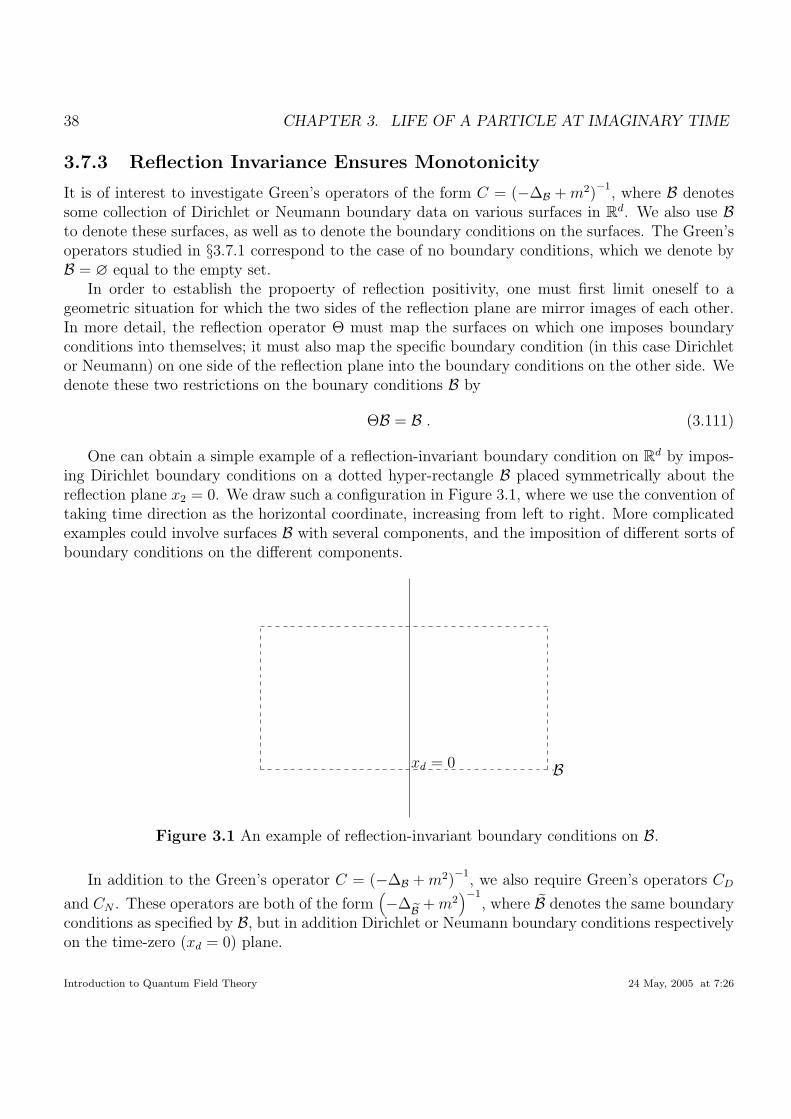
38 CHAPTER 3. LIFE OF A PARTICLE AT IMAGINARY TIME
3.7.3 Reflection Invariance Ensures Monotonicity
It is of interest to investigate Green’s operators of the form C = (−∆B +m2)−1
, where B denotessome collection of Dirichlet or Neumann boundary data on various surfaces in Rd. We also use Bto denote these surfaces, as well as to denote the boundary conditions on the surfaces. The Green’soperators studied in §3.7.1 correspond to the case of no boundary conditions, which we denote byB = ∅ equal to the empty set.
In order to establish the propoerty of reflection positivity, one must first limit oneself to ageometric situation for which the two sides of the reflection plane are mirror images of each other.In more detail, the reflection operator Θ must map the surfaces on which one imposes boundaryconditions into themselves; it must also map the specific boundary condition (in this case Dirichletor Neumann) on one side of the reflection plane into the boundary conditions on the other side. Wedenote these two restrictions on the bounary conditions B by
ΘB = B . (3.111)
One can obtain a simple example of a reflection-invariant boundary condition on Rd by impos-ing Dirichlet boundary conditions on a dotted hyper-rectangle B placed symmetrically about thereflection plane x2 = 0. We draw such a configuration in Figure 3.1, where we use the convention oftaking time direction as the horizontal coordinate, increasing from left to right. More complicatedexamples could involve surfaces B with several components, and the imposition of different sorts ofboundary conditions on the different components.
xd = 0 B
Figure 3.1 An example of reflection-invariant boundary conditions on B.
In addition to the Green’s operator C = (−∆B +m2)−1
, we also require Green’s operators CD
and CN . These operators are both of the form(−∆B +m2
)−1, where B denotes the same boundary
conditions as specified by B, but in addition Dirichlet or Neumann boundary conditions respectivelyon the time-zero (xd = 0) plane.
Introduction to Quantum Field Theory 24 May, 2005 at 7:26
3.7. REFLECTION POSITIVITY REVISITED 39
Proposition 3.7.4 (Reflection Invariance Ensures Operator Monotonicity). Assume thatC,CD, CN have the form above with boundary conditions on B satisfying ΘB = B. Then the Green’soperators are monotonic in the operator sense that
CD ≤ C ≤ CN . (3.112)
Proof. The basic idea is to give a direct proof of the monotonicity inequality
C−1N ≤ C−1 ≤ C−1
D , (3.113)
or equivalently−∆B,N ≤ −∆B ≤ −∆B,D . (3.114)
and then to use the monotonicity-reversing Lemma 3.6.2.In case that A and B are unbounded, positive, self-adjoint operators, the form domain DF (A)
is the closure of the operator domain D(A) in the norm 〈f, Af〉. The inequality A ≤ B meansDF (B) ⊂ DF (A) and
〈f, Af〉 ≤ 〈f,Bf〉 , for all f ∈ DF (B) . (3.115)
One can specify the form domain for the Laplacian with Dirichlet or Neumann boundary condi-tions. Each Laplacian is a local operator, and the three Laplace operators only differ with respectto the boundary conditions on the hyperplane t = 0. Hence we need only compare how the threeLaplacians act on functions in a neighborhood of the hyperplane t = 0. In fact, the Dirichlet Lapla-cian has fewest functions in its form domain, the free Laplacian is intermediate, and the NeumannLaplacian has the most functions,
DF (∆B,D) ⊂ DF (∆B) ⊂ DF (∆B,N) . (3.116)
For simplicity of notation, let us ignore the boundary conditions on B and concentrate on thetime-zero plane Γ = x: xd = 0. The form domain for the Laplacian ∆ are the functions
DF (∆) = f : f ∈ L2,∇f ∈ L2 . (3.117)
As long as ∇f ∈ L2, the restriction f |Γ is defined, and is an L2(Γ)-function. A similar analysisholds for one-sided derivatives. Let ∇±f denote a gradient which is two-sided on the complementof Γ and one-sided in the normal direction to Γ. The Neumann Laplacian has a form domain
DF (∆N) = f : f ∈ L2,∇±f ∈ L2 . (3.118)
These functions may have a jump continuity in the normal direction across Γ. Finally the DirichletLaplacian has a form domain
DF (∆D) = f : f ∈ L2,∇f ∈ L2, f |Γ = 0 . (3.119)
These domains satisfy 3.116, and the forms satisfy 3.114.The corresponding operators have domains
D(operator) = f : f ∈ DF , |〈∇f,∇g〉| ≤ const.‖g‖L2 . (3.120)
Integration by parts shows that this ensures for example that that normal derivative of f ∈ D(∆N)vanishes. Hence this definition coincides with the normal operator one.
Introduction to Quantum Field Theory 24 May, 2005 at 7:26
40 CHAPTER 3. LIFE OF A PARTICLE AT IMAGINARY TIME
3.7.4 Monotonicity & Reflection Positivity
The Green’s operators C = (−∆B +m2)−1
of §3.7.3 are in general complicated, and explicit formulasexist only in very special cases. For example, we can write the Green’s function for the boundarycondition illustrated in Figure 3.1 using an infinite series of image charges, reflected through alattice of hyperplanes converging to infinity. But in general, we do not attempt to give an exactformula for the Green’s function arising from a complicated set of reflection-invariant boundaries.However, once we have obtained these Green’s operators, claim that the corresponding DirichletGreen’s operator CD and the Neumann Green’s operator CN with additional Dirichlet or Neumannboundary conditions on the xd = 0 plane.
Proposition 3.7.5. Let C (−∆B +m2)−1
be a Green’s function for reflection invariant boundaryconditions ΘB = B. Then as for the elementary case, ΘC = CΘ, as well as
p±CDp± = p± (C − CΘ) p± , p±CDp∓ = 0 ,
p±CNp± = p± (C + CΘ) p± , and p±CNp∓ = 0 . (3.121)
Exercise 3.7.3. Verify Proposition 3.7.5.
As a consequence of the representations in Proposition 3.7.5, along with the operator mono-tonicity already proved in Proposition 3.7.4, we follow the proof of Proposition 3.7.2 to obtain thefollowing:
Proposition 3.7.6. Let C = (−∆B +m2)−1
be the Green’s function for reflection invariant bound-ary conditions ΘB = B. Then C is reflection positive with respect to Θ. More generally, Proposi-tion 3.7.2 holds with the more general operators C,CD, CN considered here.
3.8 Space-Time Compactification
Let us reinvestigate the ideas in the previous sections for a compact space-time. We consider herethe simplest compactification of Rd, replacing it by the torus T d with periods
` = (`1, `2, . . . , `d) . (3.122)
It is convenient to single out the time coordinate, which we denote by t = xd, and the time period,which we denote by `d = β. We parameterize the time by the interval−β/2 ≤ t ≤ β/2, with periodicboundary conditions on functions that are continuous in t, namely f(~x,−β/2) = f(~x, β/2). Weallow some periods `1, . . . , `d−1 to be infinite, in which case those coordinate directions are notcompactified. We write
Td = Td−1 × [−β/2, β/2] , (3.123)
It is often useful to consider the imbedding of L2(T d) as
L2(Td−1 × [−β/2, β/2]) ⊂ L2(Td−1 × R) . (3.124)
Introduction to Quantum Field Theory 24 May, 2005 at 7:26
3.8. SPACE-TIME COMPACTIFICATION 41
The symmetry group Td includes translations (but we lose the analog of Euclidean rotations).There are many other possibilities, but we do not consider them here.2 Let us introduce the (basis-dependent) commutative multiplication of vectors. We call this the pointwise product and use ∗ todenote this multiplication. The product a ∗ p of two vectors a, p ∈ Rd is a vector a ∗ p = p ∗ a withcomponents
(p ∗ a)i = piai . (3.125)
The torus Td is dual to a lattice Kd, which we also call the momentum space lattice. Explicitly
Kd = p : p ∗ ` ∈ 2πZd . (3.126)
This duality arises in a natural way between the Hilbert space L2(Rd) of functions f(x) on Td withthe inner product
〈f, g〉L2(Td) =∫
Tdf(x)g(x)dx , (3.127)
and the space l2(Kd) of sequences f(p) on Kd with the inner product⟨f , g
⟩l2(Kd)
=∑p∈Kd
f(p)g(p) . (3.128)
Fourier transformation F maps L2(Td)-functions to l2(Kd)-series. It has the explicit form
(Ff) (p) = f(p) =∫
Tdf(x)e−ipxdx , with p ∈ Kd . (3.129)
Then the inverse transformation is(F−1f
)(x) =
1
v1/2
∑p∈Kd
f(p)eipx , (3.130)
where v denotes the volume of the d-torus, v =∏d
i=1 `i. With this normalization, F is an isomorphismas a map between L2(Td) and l2(Kd), and
〈f, g〉L2(Td) = 〈Ff,Fg〉l2(Kd) . (3.131)
3.8.1 Periodic Green’s Function
Here we define the Green’s function and Green’s operator for a Laplace operator that is periodicin space and time. In the limit that a period `j (either in a spatial direction or the time direction)becomes infinite, this Laplacian converges to the ordinary free Laplacian with respect to thatcoordinate direction.
2Even in d = 2 one might consider the multitude of space-times given by Riemann surfaces or other surfaces withsingularities. The care of Riemann surfaces that are Shottky doubles, with identical components on each side of thetime-zero plane has been studied in some detail.
Introduction to Quantum Field Theory 24 May, 2005 at 7:26
42 CHAPTER 3. LIFE OF A PARTICLE AT IMAGINARY TIME
The Laplacian ∆T on Td, and the corresponding Green’s operator CT = (−∆T +m2)−1
whichacts on L2(Td). Here
∆T =d∑
j=1
∂2
∂x2j
. (3.132)
We also consider Td as a d-dimensional rectangle Id imbedded in Rd with the jth side length `j, andwith opposite faces identified. We can also regard functions f ∈ L2(Td) as functions on Rd satisfyperiodic boundary conditions
f(x+ n ∗ `) = f(x) , for n ∈ Zd . (3.133)
The L2(Td) inner product is obtained by restriction of L2(Rd) to L2(Id). Using this representationwe read off the formula for the Green’s operator CTd and the Green’s function CTd(x; y).
Proposition 3.8.1. The Green’s functions for the periodic Laplacian on L2(Td) is
CT(x− y) =∑
n∈Zd
C(x− y + n ∗ `) . (3.134)
One can denote the corresponding Green’s operator as
CT =∑
n∈Zd
Tn∗`C , restricted to L2(Id) , (3.135)
Proof. Note that the sum (3.134) converges due to the exponential decay of the free Green’s func-tion C on L2(Rd). This is a consequence of the assumption of positive mass, m > 0. Consequently,as any period `j tends to infinity, the sum in that coordinate direction tends to the single termwithout translation, yielding free boundary conditions in that coordinate direction. The resultingsum satisfies the Green’s function equation and also has the appropriate periodics. Therefore it isthe periodic Green’s function. The representation of the Green’s operator is just an interpretationof the formula for the Green’s function.
3.8.2 Periodic Time Reflection
One would also like to introduce time-reflection on Td or Id, and this requires the proper interpre-tation of time reflection. We regard the time coordinate in Id as a periodic interval in the line,parameterized by −β/2 ≤ t ≤ β/2. When we take the time-reflection to occur relative to t = 0.The “positive-time” and “negative-time” time half-spaces by
Id+ = Id−1 × [0, β/2] , and Id
− = Id−1 × [−β/2, 0] . (3.136)
Then Id = Id− ∪ Id
+. The time reflection acts on the d-brane Id as
Θ(~x, t) = (~x,−t) , (3.137)
Introduction to Quantum Field Theory 24 May, 2005 at 7:26
3.8. SPACE-TIME COMPACTIFICATION 43
so
ΘId± = Id
∓ . (3.138)
The Jacobian of the change of coordinates x→ Θx on Id has magnitude 1, so the isomorphism Θof Id defines a unitary transformation of L2(Id) into itself. We also use the symbol Θ to denotethis unitary. Furthermore
L2(Id) = L2(Id−)⊕ L2(Id
+) , (3.139)
the unitary Θ has the property that
ΘL2(Id±) = L2(Id
∓) . (3.140)
Exactly the same relations hold on the torus Td. We define positive-time and negative-timesubspaces
Td+ = Td−1 × [0, β/2] , Td
− = Td−1 × [−β/2, 0] , and Td = Td− ∪ Td
+ , (3.141)
and a time-reflection operator Θ such that
ΘTd± = Td
∓ , and ΘS = S , (3.142)
where S = Td− ∩ Td
+ is the time-reflection invariant (d − 1)-dimensional surface which one mightalso call a p-brane. Also
L2(Td) = L2(Td−)⊕ L2(Td
+) . (3.143)
The operator Θ is unitary and idempotent on L2(Td) and has the property that
ΘL2(Td±) = L2(Td
∓) . (3.144)
One can picture this geometric configuration by imbedding the torus Td in R2d. Represent Td
by Id with opposite sides identified. Denote the coordinates on Td by x and the coordinates on R2d
by y. Orient Td in R2d so that the first coordinate is parameterized by x1 ∈ [−`1/2, `1/2] with theendpoints identified; in the imbedding this coordinate increases counter-clockwise around a circleS1 lying in the plane y1 y2. The circle has circumference `1 and we place its center at the origin ofRd+1. Represent the jth coordinate xj of Td as a circle of circumference `j centered at the origin ofthe y2j−1 y2j-plane. Parameterize the time coordinate t = xd by the interval t ∈ [−β/2, β/2]. ThenΘ satisfies (3.137).
We draw this schematically Figure 3.2, in which we illustrate a cross-section of the plane y2d−1 y2d.In the case d = 1, this gives the exact picture. For convenience, we depict the coordinate y2d
horizontally and increasing to the right, while we draw the coordinate y2d−1 in the vertical direction.We take the point t = ∓β/2 to lie on the positive y2d-axis and the point t = 0 to lie on the negativeyd-axis. The coordinates y1, . . . , y2d−2 are orthogonal to the cross-section that we illustrate.
Introduction to Quantum Field Theory 24 May, 2005 at 7:26
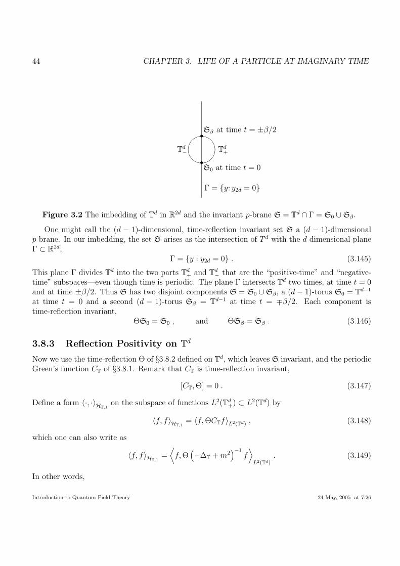
44 CHAPTER 3. LIFE OF A PARTICLE AT IMAGINARY TIME
&%'$s
sS0 at time t = 0
Sβ at time t = ±β/2
Td+Td
−
Γ = y: y2d = 0
Figure 3.2 The imbedding of Td in R2d and the invariant p-brane S = Td ∩ Γ = S0 ∪Sβ.
One might call the (d − 1)-dimensional, time-reflection invariant set S a (d − 1)-dimensionalp-brane. In our imbedding, the set S arises as the intersection of T d with the d-dimensional planeΓ ⊂ R2d,
Γ = y : y2d = 0 . (3.145)
This plane Γ divides Td into the two parts Td+ and Td
− that are the “positive-time” and “negative-time” subspaces—even though time is periodic. The plane Γ intersects Td two times, at time t = 0and at time ±β/2. Thus S has two disjoint components S = S0 ∪Sβ, a (d− 1)-torus S0 = Td−1
at time t = 0 and a second (d − 1)-torus Sβ = Td−1 at time t = ∓β/2. Each component istime-reflection invariant,
ΘS0 = S0 , and ΘSβ = Sβ . (3.146)
3.8.3 Reflection Positivity on Td
Now we use the time-reflection Θ of §3.8.2 defined on Td, which leaves S invariant, and the periodicGreen’s function CT of §3.8.1. Remark that CT is time-reflection invariant,
[CT,Θ] = 0 . (3.147)
Define a form 〈·, ·〉HT,1on the subspace of functions L2(Td
+) ⊂ L2(Td) by
〈f, f〉HT,1= 〈f,ΘCTf〉L2(Td) , (3.148)
which one can also write as
〈f, f〉HT,1=⟨f,Θ
(−∆T +m2
)−1f⟩
L2(Td). (3.149)
In other words,
Introduction to Quantum Field Theory 24 May, 2005 at 7:26
3.8. SPACE-TIME COMPACTIFICATION 45
Proposition 3.8.2. On the Hilbert space L2(Td+), the operator CT is reflection positive with respect
to Θ. In other words, the form 〈·, ·〉HT,1is positive semi-definite, namely
0 ≤ 〈f, f〉HT,1= 〈f,ΘCTf〉L2(Td) , for all f ∈ L2(Td
+) . (3.150)
Proof. We show that reflection positivity for CTd on L2(Td+) is a consequence of reflection positivity
of C on L2(Rd+), established in Proposition 3.3.2. Use the representation of functions in Td as
functions on Td−1 ×R, periodic in time with period β and with −β/2 ≤ t ≤ β/2 being the domainfor the L2(Td) inner product. Define the spatially-periodic Green’s function
CP (x− y) =∑
~n∈Zd−1
C(x− y + (~n ∗ ~, 0)) , so CTd(x− y) =∑j∈Z
CP (x− y + (~0, jβ)) . (3.151)
The operator CP acts on L2(Td−1 × R). Since C is reflection positive, it C commutes with Θ andwith spatial translations T~n∗~. But T~n∗~ also commutes with Θ. From this we infer that CP isreflection positive with respect to Θ.
For shorthand, writeT~x = T(~x,0) , and Tt = T(~0,t) . (3.152)
Hence we need only analyze the sum in (3.135) over translation in the time direction. For f ∈L2(Td
+), write
〈f, f〉HT,1=∑j∈Z
〈f,ΘTjβCPf〉L2(Td−1×R) . (3.153)
We claim that each individual term in the sum (3.153) is positive. For a term with j ≥ 0, use thefact that Tjβ commutes with CP and TjβΘ = ΘT−jβ to give
〈f,ΘTjβCPf〉L2(Td−1×R) =⟨Tjβ/2f,ΘCPTjβ/2f
⟩L2(Td−1×R)
≥ 0 . (3.154)
Here we use Tjβ/2f ∈ L2(Rd+) and that CP is reflection positive with respect to Θ.
On the other hand, for terms with j < 0,
〈f,ΘCPTjβf〉L2(Td−1×R) =⟨T−jβ/2Θf, Tjβ/2CPf
⟩L2(Td)
=⟨(T−jβ/2Θf
),ΘCP
(T−jβ/2Θf
)⟩L2(Td−1×R)
≥ 0 . (3.155)
In the final step we use the fact that f ∈ Td−1×I+; therefore the translates(T−jβ/2Θf
)in question
with j ≤ −1 lie in L2(Td−1×R+). The positivity of (3.155) then follows from the reflection positivityof CP with respect to Θ. Combining the results of (3.154)–(3.155), we conclude that each term in(3.153) is positive, and the proof is complete in this case. The general case follows by using ωT asthe appropriate energy operator on Td−1.
We can extend this computation in a straight-forward way to give
Proposition 3.8.3. For f, g ∈ L2(Td+) and 0 ≤ t ≤ β, we compute 〈f, Ttg〉HT,1
=⟨f , Ttg
⟩HT,1
as
〈f, Ttg〉HT,1=
∞∑j=0
(〈f,ΘCPTt+jβ g〉L2(Td−1×R) +
⟨(Tβ/2Θf
),ΘCPTt+jβ
(Tβ/2Θf
)⟩L2(Td−1×R)
)(3.156)
Introduction to Quantum Field Theory 24 May, 2005 at 7:26
46 CHAPTER 3. LIFE OF A PARTICLE AT IMAGINARY TIME
3.8.4 Quantization on Td and the Role of S = ΘS
We use the reflection-positive form 〈·, ·〉HT,1on L2(Td
+) to define a Hilbert space of quantum-mechanical states and quantized operators acting on these states. This is the space
HT,1 = L2(Td+)/N = f + g : f ∈ L2(Td
+) , and g ∈ N , (3.157)
where N is the null space of 〈·, ·〉HT,1.
Introduce the Sobolev space H−1(O; Td) in analogy with (3.158), as the Hilbert space of gener-alized functions f on Td of the form
H−1
(O; Td
)= f : C
1/2T f ∈ L2(Td) , and support f ⊂ O . (3.158)
This space is a Hilbert space with the inner product
〈f, g〉H−1=⟨C
1/2T f, C
1/2T g
⟩L2(Td)
. (3.159)
One can follow the construction of the quantization map ∧ in §3.4, except we do not have as manysymmetries of Td
+ as of Rd+. We obtain
∧: H−1(Td+) 7→ HT,1 , or HT,1 =
(H−1(Td
+))∧
. (3.160)
We begin with the identification of the this Hilbert space as a Sobolev space. Let ∇2Td−1 denote
the Laplace operator on the (d− 1)-dimensional torus Td−1, and let ωT =(∇2
Td−1 +m2)1/2
. Define
the Sobolev space H−1/2(Td−1) as the Hilbert space of generalized functions f on Td−1 with the innerproduct
〈f, g〉H−1/2(Td−1) =⟨(2ωT)−1/2
f, (2ωT)−1/2g⟩
L2(Td−1). (3.161)
Note that generalized functions f⊗ δs with fH−1/2(Td−1) and localized at a sharp time s ∈ [0, β/2]are elements of , H−1(Td
+).
Proposition 3.8.4 (Identification of the Inner Product). The quantization(H−1/2(Td−1)⊗ δt
)∧of H−1/2(Td−1)⊗ δt ⊂ H−1(Td
+) for any fixed t ∈ [0, β/2] is dense in HT,1. Furthermore, the scalarproduct of the quantization of two such functions of the form f⊗ δt is⟨
(f⊗ δt)∧ , (g⊗ δs)
∧⟩HT,1
=⟨f, e−(t+s)ωT coth(βωT/2) g
⟩H−1/2(Td−1)
. (3.162)
Remark 3.8.5. The norm of the quantization of sharp-time functions is equivalent to theH−1/2(Td−1) norm, in the sense that there is a constant M such that
‖f‖H−1/2(Td−1) ≤∥∥∥(f⊗ δt)
∧∥∥∥HT,1
≤M ‖f‖H−1/2(Td−1) . (3.163)
Introduction to Quantum Field Theory 24 May, 2005 at 7:26
3.8. SPACE-TIME COMPACTIFICATION 47
In fact using (3.162) we infer that the norm of sharp-time function is∥∥∥(f⊗ δt)∧∥∥∥HT,1
= 〈f, coth(βωT/2) f〉1/2
H−1/2(Td−1) . (3.164)
As m ≤ ωT, the spectral theorem shows that
I ≤ coth(βωT/2) ≤ coth(βm/2) = M2 , (3.165)
from which the remark follows.
Remark 3.8.6. This result shows that the quantization Tt of time translation Tt for 0 ≤ t ≤ β/2is the self-adjoint contraction e−tωT. These operators extend to a semi-group for all t ≥ 0.
Remark 3.8.7. A new feature of periodic time is the possibility that the Hilbert spaces generatedby the quantization of functions localized on each of the disjoint components of S are distinct.However, the two components of S arise from localization at time t = 0 and at time t = β/2. Theproposition shows that quantization of functions f localized on each of the two disjoint components
S0 and Sβ of S yield a dense set of the entire Hilbert space HT,1 =(H−1(Td
+))∧
.
Proof. First consider the case with all spatial periods infinite, so Td−1 becomes Rd−1, and Td =Rd−1 × [−β/2, β/2]. Suppose t ≥ 0. We use result of Proposition 3.8.3 to compute the matrix
element 〈f, Ttg〉HT,1=⟨f , Ttg
⟩HT,1
. For f, g ∈ H−1(Td+),
⟨f , Ttg
⟩HT,1
= 〈f, Ttg〉HT,1
=∞∑
j=0
(〈f,ΘCPTt+jβ g〉L2(Td−1×R) +
⟨(Tβ/2Θf
),ΘCPTt+jβ
(Tβ/2Θg
)⟩L2(Td−1×R)
)
=∞∑
j=0
⟨f , e−(t+jβ)ωT g
⟩HT,1
+∞∑
j=0
⟨(Tβ/2Θf
)∧, e−(t+jβ)ωT
(Tβ/2Θg
)∧⟩HT,1
=⟨f , e−tωT
(I − e−βωT
)−1g⟩HT,1
+⟨(Tβ/2Θf
)∧, e−tωT
(I − e−βωT
)−1 (Tβ/2Θg
)∧⟩HT,1
. (3.166)
Note that Tβ/2ΘTd+ ⊂ Td
+, so the function Tβ/2Θf has a quantization.Now let us specialize to functions f = f⊗ δ, g = g⊗ δ and t replaced by t+ s, corresponding to
localizing f at time t and g at time s. We simplify the two terms on the right of (3.166). As in theproof of Proposition 3.4.4, the first term is just⟨
f, e−(t+s)ωT(I − e−βωT
)−1g
⟩H−1/2(Td−1)
. (3.167)
Introduction to Quantum Field Theory 24 May, 2005 at 7:26
48 CHAPTER 3. LIFE OF A PARTICLE AT IMAGINARY TIME
The second term simplifies as both f and g are localized at time zero, and thus time reflectioninvariant. This term then becomes⟨
f, e−(t+s+β)ωT(I − e−βωT
)−1g
⟩H−1/2(Td−1)
. (3.168)
Adding these two results yields the inner products (3.162).
We now establish that the states at t = 0 span HT,1 =(H−1(Td
+))∧
. Write f ∈ H−1(Td+) as a
superposition of functions localized at time s ∈ [0, β/2],
f =∫ β/2
0fs ⊗ δsds , where fs(~x) = f(~x, s) . (3.169)
Likewise,
Tβ/2Θf =∫ β/2
0fβ/2−s ⊗ δsds =
∫ β/2
0fs ⊗ δβ/2−sds . (3.170)
Then we can use the contributions to the sharp-time inner product to write
⟨f , g
⟩HT,1
=∫ β/2
0
∫ β/2
0
⟨fs, e
−(s+s′)ωT(I − e−βωT
)−1gs′
⟩H−1/2(Td−1)
dsds′
+∫ β/2
0
∫ β/2
0
⟨fs, e
−(β−s−s′)ωT(I − e−βωT
)−1gs′
⟩H−1/2(Td−1)
dsds′ .
(3.171)
If we write
f+ =∫ β/2
0e−sωT fsds , and f− =
∫ β/2
0e−(β/2−s)ωT fsds , (3.172)
then we have⟨f , g
⟩HT,1
=⟨f+,
(I − e−βωT
)−1g+
⟩H−1/2(Td−1)
+⟨f−,
(I − e−βωT
)−1g−
⟩H−1/2(Td−1)
.
(3.173)
Now we localize g to a fixed time t ∈ [0, β/2], by taking it of the form gt = g ⊗ δt withg ∈ H−1/2(Td−1). The inner product of such a gt with a general f ∈ H−1(Td
+) becomes⟨f , gt
⟩HT,1
=⟨f , (g⊗ δt)
∧⟩HT,1
=⟨f+, e
−tωT(I − e−βωT
)−1g
⟩H−1/2(Td−1)
+⟨f−, e
−(β/2−t)ωT(I − e−βωT
)−1g
⟩H−1/2(Td−1)
.
(3.174)
Introduction to Quantum Field Theory 24 May, 2005 at 7:26
3.9. MIRROR SPACE-TIME LATTICE 49
Let us assume that functions of the form gt ∈(H−1/2(Td−1)⊗ δt
)∧, for fixed t ∈ [0, β/2], do
not span HT,1. In this case there is a function f ∈ G−1(Td+) 6∈ N orthogonal to such gt, so (3.174)
vanishes for all gt. In this case, choose
g = e−tωT f+ + e−(β/2−t)ωT f− . (3.175)
For this particular g, ⟨f , gt
⟩HT,1
=⟨g,(I − e−βωT
)−1g⟩
H−1/2(Td−1)= 0 . (3.176)
But ωT ≥ m, so S =(I − e−βωT
)−1satisfies
1 ≤ S ≤ (1− e−βm)−1 . (3.177)
In particular S is bounded and has a bounded inverse, so S has no null vectors. We thereforeconclude that f = 0, or f ∈ N . This completes the proof.
We remark that we have in the course of this proof given a nice expression for the inner product⟨f , g
⟩HT,1
between two general functions in L2(Td+).
Corollary 3.8.8. For f, g ∈ H−1(Td+), one has⟨
f , g⟩HT,1
=⟨f+,
(I − e−βωT
)−1g+
⟩H−1/2(Td−1)
+⟨f−,
(I − e−βωT
)−1g−
⟩H−1/2(Td−1)
, (3.178)
with f± defined in (3.172).
3.9 Mirror Space-Time Lattice
One way to treat ultra-violet regularization is to replace Euclidean space-time by a lattice space-time Kd. Discretization of space-time is dual to compactification studied in the previous section.However, now we introduce the lattice Laplacian as the fundamental operator and we considersymmetries of the lattice as fundamental symmetries of space-time.
In this case it is natural to take a cubic lattice with equal spacing δ in each coordinate direction.Denote a space-time coordinate by x ∈ Kd and a function on space-time by a series f(x) for x ∈ Kd.This space is dual to a momentum space torus Td with equal periods `j = 2π
δ.
3.9.1 Green’s Functions
3.9.2 Time Reflection
3.9.3 Reflection Positivity
Introduction to Quantum Field Theory 24 May, 2005 at 7:26

50 CHAPTER 3. LIFE OF A PARTICLE AT IMAGINARY TIME
Introduction to Quantum Field Theory 24 May, 2005 at 7:26

Part II
Fock Space
51

53
The Hilbert space of a free quantum field is called Fock space. We develop the elementarynotions of this Hilbert space, as well as deriving some properties of standard operators on thisspace. For readers new to quantum field theory, this chapter is more or less self-contained. Othersmay wish to scan this part of the book for notation, and proceed quickly to the later parts. Tobegin, we review here some basic properties of Hilbert spaces and linear transformations (also called“operators”) on Hilbert space.
In Schrodinger quantum theory, the wave function for a spinless boson with coordinates ~x1 isdescribed by a wave functions f1(~x1). The wave function for two particles at ~x1 and ~x2 is describedby a composite wave function functions that is the product of the wave function for each particle,f1(~x1)f2(~x2). This product is a tensor product wave function. So tensor products will play a keyrole in understanding the Hilbert space of n-particles.
In order to take into account the indistinguishability of bosons, one symmetrizes the wavefunction of two bosons to have the form f1(~x1)f2(~x2)+ f2(~x1)f1(~x2). Correspondingly fermionic two-particle states are anti-symmetric, having the form f1(~x1)f2(~x2)− f2(~x1)f1(~x2). For example, if onechooses the Hilbert space H for single particle wave functions to be the appropriate space H−1/2(Rs)for a massive, spinless boson, as introduced in (2.54), then a two-particle wave functions will lie inthe tensor product H−1/2(Rs)⊗ H−1/2(Rs).
In the case of some other type of particle, if the one-particle wave functions lie in H, then thetwo particle wave function lies in H⊗H. One also needs to take into account the type of particle,and to symmetrize or anti-symmetrize the tensor product. For example, in the case of two spinlessbosons, one wants to restrice the space of two-particle states from the entire tensor product to thesymmetric tensor product H−1/2(Rs) ⊗s H−1/2(Rs). On the other hand, in the case of fermions onthe one-particle space H, then one takes the anti-symmetric tensor product H ∧H.
Fock space results from generalizing these ideas to describe an arbitrary number of particles.The two representations of the symmetric group corresponding to complete symmetry and completeanti-symmetry play a special role in physics: all particles observed to date in nature appear tobe either bosons or fermions. The famous “spin and statistics” theorem of relativistic quantumfield theory does not say that these are the only allowed possibilites; rather it makes the weakerstatement that special relativity and positive energy are incompatible with anti-symmetrized bosonsor symmetrized fermions.
In general, we consider a Hilbert space that describes an arbitrary number of particles, each ofthe form of a single particle given by states in F1. For a single type of particle, this Hilbert spaceis a sum
F = ⊕∞n=0Fn , (3.179)
where Fn is the space of states for exactly n particles. We also write this as
F = expH , (3.180)
where a natural exponential emerges relating the one-particle space H to the Fock space describingan arbitrary number of particles.
Introduction to Quantum Field Theory 24 May, 2005 at 7:26

54
Introduction to Quantum Field Theory 24 May, 2005 at 7:26
Chapter 4
Sums and Products
Tensor products arise early in the study of quantum theory. As soon as one analyzes a particlewith spin in Schrodinger Theory, or several particles with or without spin, one meets a tensorproduct wave function. The Hilbert space for a particle with spin is the tensor product of the basicone-particle space F1 with a finite dimensional spin space CN . Thus the wave function of a singleparticle with spin has the form fi(~x), where i indexes the finite-dimensional spin space. The spinspace is one-dimensional for spin zero, corresponding to the case of F1.
Before delving into the details of the state space for a particular particle or field, we consider inthis chapter some general properties of the tensor products that we will meet in later chapters. Weconstruct a tensor algebra over a Hilbert space H. Two particular subalgebras, one with symmetricmultiplication and the other with anti-symmetric multiplication, correspond to the Fock spaces forbosons and fermions respectively.
4.1 The Direct Sum
The direct sum of two Hilbert spaces K1 and K2 is the Hilbert space
K1 ⊕K2 , (4.1)
defined as pairs of vectors f1, f2 with fj ∈ Kj. The scalar product of two vectors in the directsum is
〈f1, f2, g1, g2〉K1⊕K2= 〈f1, g1〉K1
+ 〈f2, g2〉K2. (4.2)
There is a permutation transformation τ12 such that τ 212 = I with the property that
τ12 : K1 ⊕K2 = K2 ⊕K1 . (4.3)
Clearly the sum ⊕ is associative
(K1 ⊕K2)⊕K3 = K1 ⊕ (K2 ⊕K3) . (4.4)
The direct sum often arises in considering several copies of the same or similar transformations(such as fields with components).
55
56 CHAPTER 4. SUMS AND PRODUCTS
4.2 The Tensor Product
The tensor product of two Hilbert spaces K1 and K2 is a new Hilbert space K1 ⊗K2.
4.2.1 Definition of K1 ⊗K2
Define the elementary elements of the space K1 ⊗K2 as pairs of vectors f1 ∈ K1 and f2 ∈ K2,written as f1 ⊗ f2. For λ ∈ C, one identifies λ(f1 ⊗ f2) = (λf1) ⊗ f2 = f1 ⊗ (λf2), and considersformal sums of vectors of these elementary vectors. One takes the inner product of two elementaryvectors in K1 ⊗K2 as the product of the corresponding inner products,
〈f1 ⊗ f2, g1 ⊗ g2〉K1⊗K2= 〈f1, g1〉K1
〈f2, g2〉K2. (4.5)
One extends this definition by linearity to finite sums of k1k2 elementary vectors
Ω =k1∑
α1=1
k2∑α2=1
cα1α2 fα11 ⊗ fα2
2 , where cα1α2 ∈ C . (4.6)
These vectors comprise the algebraic tensor product.The inner product of two such vectors Ω and Ω′ must be linear in Ω′ and conjugate linear in Ω.
Thus for any choice of k1 vectors fαj
1 ∈ K1 and k2 vectors fαj
2 ∈ K2 the inner product must havethe form
〈Ω,Ω′〉K1⊗K2=
∑αα′
cα cα′⟨fα1
1 ⊗ fα22 , g
α′11 ⊗ g
α′22
⟩K1⊗K2
=∑αα′
cα cα′⟨fα1
1 , gα′11
⟩K1
⟨fα2
2 , gα′22
⟩K2
. (4.7)
Here one denotes α = (α1, α2) as a multi-index. The condition that this form make K1 ⊗K2 intoa pre-Hilbert space is the statement that 0 ≤ 〈Ω,Ω〉, with vanishing only possible if Ω = 0. Inother words, the form (4.7) is positive definite on (K1 ⊗K2)× (K1 ⊗K2). In this case, the algebraictensor product K1 ⊗K2 is a pre-Hilbert space that can be completed to a Hilbert space that wecall K1 ⊗K2.
Proposition 4.2.1. The form (4.7) is positive definite.
Proof. Define M and N as k1 × k1 and k2 × k2 hermitian matrices with entries
Mα1α′1=⟨fα1
1 , fα′11
⟩, and Nα2α′2
=⟨fα2
2 , fα′22
⟩. (4.8)
Then〈Ω,Ω〉 =
∑αα′
cα Mα1α′1Nα2α′2
, cα′ , (4.9)
In other words we need to study the positivity of k1k2-dimensional square matrices with entriesMα1α′1
Nα2α′2.
Introduction to Quantum Field Theory 24 May, 2005 at 7:26
4.2. THE TENSOR PRODUCT 57
On the Hilbert space K1, the existence of the inner product is equivalent to the statementthat all matrices of the form M are positive, and the statement that the vectors fα1
1 are linearlyindependent, is equivalent to the matrix M being positive definite. The same is true for K2 andmatrices of the form N . Therefore, the requirement that (4.9) is an inner product is that the matrixk1k2 × k1k2 matrix K = M ⊗N defined by the matrix elements
Kαα′ = Mα1α′1Nα2α′2
(4.10)
is positive.If we choose the fα1
1 to be linearly independent in K1, and the fα22 to be linearly independent in
K2, one wants the fα11 ⊗fα2
2 to be linearly independent in K1 ⊗K2. This is equivalent to the matrixK being positive definite when M and N are positive definite. If this is the case, then K1⊗K2 is apre-Hilbert space; it can be turned into a Hilbert space by completing it in the given inner product.In other words, it is sufficient to establish the following:
Proposition 4.2.2. Consider hermitian, positive matrices M and N with matrix elements Mα1α′1and dimension k1 × k1, and matrix elements Nα2α′2
and dimension k2 × k2 respectively. Then thek1k2 × k1k2 matrix K = M ⊗ N defined by the matrix elements (4.10) is positive. Furthermore ifM and N are positive definite, then K is positive definite.
Proof. Since Mα1α′1is hermitian, there is a an orthonormal basis of eigenvectors f (1), . . . , fk1 ∈ Ck1
with components f (j)α1
and eigenvalues 0 ≤ λj. Similarly there is an orthonormal basis of eigenvectors
g(j′) ∈ Ck2 , with 1 ≤ j ≤ k2 for N , with eigenvalues µj′ . Note that the orthonormal vectors withcomponents f (j)
α1g(j′)
α2are eigenvectors for K with eigenvalues 0 ≤ λjµj′ . There are exactly k1k2 such
vectors, so they give an orthonormal basis for Ck1k2 . Therefore K is positive. Furthermore, if eachλj and µj′ is strictly positive, so is each eigenvalue λjµj′ .
SPECIFIC CASES Example 1. As we see from the proof above, the Hilbert space Rd1⊗Rd2 =Rd1d2 , and likewise Cd1 ⊗ Cd2 = Cd1d2 . For finite dimensional Hilbert spaces,
dim (K1 ⊗K2) = dimK1 × dimK2 . (4.11)
Example 2. In case we choose an orthonormal bases e(α1)1 ∈ K1 and e
(α2)2 ∈ K2, then e(α1) ⊗ e
(α2)2
is an orthonormal basis for K1 ⊗K2. The expansion
f =∑α1α2
cα1α2 e(α1)1 ⊗ e
(α2)2 , with cα1α2 =
⟨e(α1)1 ⊗ e
(α2)2 , f
⟩K1⊗K2
, (4.12)
gives〈f, f ′〉K1⊗K2
=∑α1α2
cα1α2c′α1α2
. (4.13)
Example 3. The tensor product of two L2(Rd) spaces obeys the rule
L2(Rd1)⊗ L2(Rd2) = L2(Rd1+d2) . (4.14)
Introduction to Quantum Field Theory 24 May, 2005 at 7:26
58 CHAPTER 4. SUMS AND PRODUCTS
Properties of the Hilbert space L2(Rd) can be understood in terms of an orthonormal basis ofeigenfunctions for the oscillator with d-components. These eigenfunctions factorize into (tensor)products of one-dimensional eigenfunctions, as does the measure of integration, dq, leading to thestated relation.
Example 4. The Sobolev Hilbert space H−1(Rd) introduced in (3.51) displays another behavior,namely
H−1(Rd1)⊗ H−1(Rd2) % H−1(Rd1+d2) . (4.15)
In Fourier space, the inner product in H−1(Rd) is given by the measure
1
p2 +m2dp . (4.16)
The weight factor (p2 + m2)−1 in dimension d1 + d2 does not factorize into the product of weightfactors in dimension d1 and d2. Thus in the case d1 = d2 = 1, for example, the generalized functionδ ∈ H−1(R). Therefore δ ⊗ δ belongs to the two-particle space,
δ ⊗ δ ∈ H−1(R)⊗ H−1(R) , however δ ⊗ δ 6∈ H−1(R2) . (4.17)
Example 5. One can apply the tensor product construction to spaces with other topologies,such as the countably-normed Schwartz space S(Rd), with norms (??). Giving the algebraic tensorproduct the topology induced from this countable set of norms, one has
S(Rd1)⊗ S(Rd1) = S(Rd1+d2) . (4.18)
4.2.2 Tensor Products of Operators
Two linear transformationA1 onK1 andA2 onK2 respectively, yield a tensor product transformationA1 ⊗ A2 that acts on K1 ⊗K2. Explicitly one defines
(A1 ⊗ A2) (f ⊗ g) = (A1f)⊗ (A2g) , (4.19)
and extends this definition by linearity to all of K1 ⊗K2. As a consequence,
(A1 ⊗ A2) (A′1 ⊗ A′2) = (A1A′1)⊗ (A2A
′2) , (4.20)
and(A1 ⊗ A2)
∗ = A∗1 ⊗ A∗2 . (4.21)
Consequently,(A1 ⊗ A2)
∗ (A1 ⊗ A2) = (A∗1A1)⊗ (A∗2A2) . (4.22)
The matrix elements of A1⊗A2 in the basis ei1 ⊗ fi2 can be expressed in terms of the matrixelements of A1 in the basis ei1 and A2 in the basis fi2, namely
(A1)i1j1= 〈ei1 , A1ej1〉K1
, and (A1)i2j2= 〈fi2 , A2fj2〉K2
. (4.23)
Introduction to Quantum Field Theory 24 May, 2005 at 7:26
4.2. THE TENSOR PRODUCT 59
Then
(A1 ⊗ A2)i1i2,j1j2= 〈ei1 ⊗ fi2 , (A1 ⊗ A2) (ej1 ⊗ fj2)〉K1⊗K2
= (A1)i1j1(A2)i2j2
. (4.24)
On general vectors g ∈ K1 ⊗K2 of the form (4.6),
((A1 ⊗ A2) g)i1i2=∑j1,j2
(A1)i1j1(A2)i2j2
gj1j2 . (4.25)
We establish two fundamental properties of the tensor product A1⊗A2 of two transformations.These two properties concern certain upper and lower bounds that we often encounter.
Proposition 4.2.3. Let A1, A2 be bounded transformations on Hilbert spaces K1 and K2 respectively,and let A1 ⊗ A2 be defined as above on K1 ⊗K2.
i) The operator norm of A1⊗A2 on K1 ⊗K2 is given by the product of the norms of the factors,
‖A1 ⊗ A2‖K1⊗K2= ‖A1‖K1
‖A2‖K2. (4.26)
ii) If 0 ≤ A1 and 0 ≤ A2 each are positive, then the tensor product transformation is also positive,
0 ≤ A1 ⊗ A2 . (4.27)
iii) The transformation A1⊗ I has a bounded inverse on K1⊗K2 if and only if A1 has a boundedinverse on K1. In that case,
(A1 ⊗ I)−1 = A−11 ⊗ I . (4.28)
iv) The spectrum of A1 ⊗ I on K1 ⊗K2 coincides with the of A1 on K1.
Proof. Any bounded transformation T on a Hilbert space K can be approximated strongly by asequence Tn of finite rank transformations obtained by projecting T onto an n-dimensional subspaceof K, with ‖Tn‖K → ‖T‖K. Thus it is sufficient to establish the proposition for A1 and A2 equal tofinite dimensional matrices. Furthermore, any transformation T on a Hilbert space satisfies the C∗
property ‖T‖ = ‖T ∗T‖1/2, so
‖A1 ⊗ A2‖K1⊗K2= ‖A∗1A1 ⊗ A∗2A2‖1/2
K1⊗K2. (4.29)
As a consequence, it is sufficient to restrict attention to proving (4.26) for positive A1 and A2, as weassume also for (4.27). Thus it is convenient to take ei1 to be an orthonormal basis of eigenfunc-tions of A1 with eigenvalues λi1 and to take fi2 to be an orthonormal basis of eigenfunctions of A2
with eigenvalues µi2 . As a consequence, the vectors ei1 ⊗ fi2 are an orthonormal basis eigenvectorsof A1 ⊗A2 with eigenvalues λi1µi2 . But this shows that for each finite dimensional approximation,all the eigenvalues of A1 ⊗ A2 are positive, and also that
‖A1 ⊗ A2‖K1⊗K2= sup
i1,i2
λi1µi2 = ‖A1‖K1‖A2‖K2
. (4.30)
Introduction to Quantum Field Theory 24 May, 2005 at 7:26
60 CHAPTER 4. SUMS AND PRODUCTS
This completes the proof of (ii). If the inverse of A1 exists, then the multiplication law (4.20) showsthat A−1
1 ⊗ I is the inverse of A1 ⊗ I. The spectrum of T is the complement of the set for whichT − λI has a bounded inverse. But
(A1 ⊗ I)− λ (I ⊗ I) = (A1 − λI)⊗ I , (4.31)
so parts (iii) and (iv) also follow.
4.2.3 The Pointwise Operator Product
The pointwise operator product A ∗B is a restriction of the tensor product A⊗B of operators onH ⊗ H to a subspace isomorphic to H. When H is finite dimensional, the pointwise product ofbounded transformations A,B always define a bounded transformation A∗B. This may not be thecase when H is infinite-dimensional case.
In an earlier discussion, we found it useful to introduce a basis-dependent, pointwise productof vectors f ∗ g. For f, g ∈ Rd, we introduced the vector f ∗ g with components (f ∗ g)i = figi,see (3.125). One could define an analogous notion on the Hilbert space `2 of square summablesequences, but in the infinite-dimensional case such a pointwise ∗-product of vectors is only definedon a subset of `2, namely for f ∈ `2 ∩ `p and g ∈ `2 ∩ `q, with 1
p+ 1
q= 1
2. On the Hilbert space of L2
functions, the pointwise product can also play a role, with (f ∗ g) (x) = f(x)g(x). But again sucha multiplication is defined only on a subspace.
It is also useful to define the pointwise product of matrices (in a particular basis). Let A,B ben×m matrices with entries Aij and Bij. Define the pointwise product A ∗B as the n×m matrixwith entries
(A ∗B)ij = AijBij . (4.32)
The corresponding nth ∗-power of A is
A∗n = A ∗ A ∗ A ∗ · · · ∗ A︸ ︷︷ ︸n-factors
(4.33)
and the ∗-exponential of A is
exp∗(A) = I +∞∑
n=1
1
n!A∗n . (4.34)
We shortly use this notion in the case of finite-dimensional matrices. But one observes that thecorresponding notion for linear transformations on an infinite-dimensional space arises for quantumfields. In particular, we have seen the central role played by the Green’s operator C = (−∆ +m2)
−1
which is a bounded linear transformation on L2(Rd), as long as m > 0. The integral kernel of thistransformation is C(x; y) = C(x − y) with the properties named in §3.2. In particular C(x; y) is
strictly positive and has a singularity on the diagonal in dimension d ≥ 3 that is ∼ |x− y|−(d−2).One can define the pointwise power C∗n of C, as the integral operator with the kernel(
C∗n)
(x; y) = C(x− y)n . (4.35)
Introduction to Quantum Field Theory 24 May, 2005 at 7:26
4.3. N -FOLD TENSOR PRODUCTS 61
Note that for
n < ncrit = d/(d− 2) . (4.36)
this kernel is locally integrable. The operator norm of C∗n on L2(Rd) is
∥∥∥C∗n∥∥∥ =
∫RdC(y)n dy <∞ , (4.37)
and C∗n defines a bounded operator on L2(Rd).On the other hand for n ≥ nc, the kernel of C∗n is not locally integrable and C∗n does not
define a bounded operator on L2(Rd). In case n ≥ ncrit, the pointwise power C∗n is said to requirerenormalization in order to be defined.
4.2.4 Pointwise Products Preserve Positivity
We saw in Exercise 3.6.1 that the functions h(t) = t2 and h(t) = et do not preserve the monotonicityof matrices when we use the usual functional calculus. However we now see that these functions dopreserve positivity, when we use the functional calculus defined by the ∗ product!
Proposition 4.2.4. Let 0 ≤ A,B be transformations on a given Hilbert space K. Then when theyare defined, the transformations A ∗B, A∗n, and exp∗(A) are all positive,
0 ≤ A ∗B , 0 ≤ A∗n , and 0 ≤ exp∗(A) . (4.38)
Remark 4.2.5. This means that if Aij and Bij are the matrix elements of self-adjoint matricesA,B with non-negative eigenvalues, then also
AijBij , (Aij)n , and eAij , (4.39)
are elements of matrices with non-negative eigenvalues.
Proof. Consider the diagonal subspace K ⊂ K⊗K of vectors of the form (??) for which gii ∈ `2.Also let K denote the orthogonal projection of K⊗K onto K. There is a natural identification of K
with K. Notice that A ∗ B is the restriction of A⊗ B on K ⊗ K to act on K. In Proposition 4.2.3we show that 0 ≤ A ⊗ B. Hence restricted to the subspace K we have 0 ≤ A ∗ B. Continuing inthis fashion, we infer 0 ≤ A∗n = A ∗ A∗n−1. Furthermore the sum of positive transformations isa positive transformation, so 0 ≤ exp∗(A).
4.3 n-Fold Tensor Products
Define the n-fold tensor product of Hilbert spaces H1, . . . ,Hn as the Hilbert space
H1 ⊗H2 ⊗ · · · ⊗ Hn , (4.40)
Introduction to Quantum Field Theory 24 May, 2005 at 7:26
62 CHAPTER 4. SUMS AND PRODUCTS
constructed as follows. Write elementary vectors in this vector space as
Ω(n)f1,...,fn
= f1 ⊗ f2 ⊗ · · · ⊗ fn , with fj ∈ Hj , (4.41)
with the inner product between two such elementary vectors (4.41) given by the product of theinner products of the individual vectors,
⟨Ω
(n)f1,...,fn
,Ω(n)g1,...,gn
⟩H1⊗H2⊗···⊗Hn
=n∏
j=1
〈fj, gj〉Hj. (4.42)
Extend the definition of vectors to be linear over C in each factor space Hj, so that finite formalsums
Ω(n) =∑α
cα Ω(n)
fα11 ,...,fαn
n, with cα ∈ C , and f
αj
j ∈ Hj . (4.43)
Here α is the multi-index α = α1, . . . , αn with 1 ≤ αj ≤ N , for some N <∞. The inner productof two such vectors Ω(n) and Ω′(n) is⟨
Ω(n),Ω′(n)⟩H1⊗H2⊗···⊗Hn
=∑α,β
cα c′β
⟨Ω
(n)fα1 ,...,fαn
,Ω(n)f ′
β1,...,f ′
βn
⟩H1⊗H2⊗···⊗Hn
. (4.44)
We see that this form (4.44) is positive definite for Ω(n) = Ω′(n) as follows. Note that
⟨Ω(n),Ω(n)
⟩H1⊗H2⊗···⊗Hn
=∑α,β
cα cβn∏
j=1
⟨fαj
, fβj
⟩Hj
. (4.45)
Hence positivity of this putative inner product is equivalent to positivity of any Nn × Nn matrixM (N,n) with matrix elements
M(N,n)α,β =
n∏j=1
M(j)αj βj
, (4.46)
where the individual matrices M (j) with matrix elements M(j)αj βj
are positive, and strictly positiveunless all the fj αj
are zero.⟨f
(n)1 , f
(n)2
⟩H1⊗H2⊗···⊗Hn
=∑
α1,...,αn
c(f(n)1 )α1···αnc(f
(n)2 )α1···αn , (4.47)
andc(f (n))α1···αn =
⟨fα1 ⊗ fα2 ⊗ · · · ⊗ fαn , f
(n)⟩H1⊗H2⊗···⊗Hn
. (4.48)
‖f1 ⊗ f2 ⊗ · · · ⊗ fn‖ =n∏
j=1
‖fj‖Hj. (4.49)
A dense set of vectors in H1⊗H2⊗ · · · ⊗Hn have the form of finite linear combinations of suchtensor products, with the vectors fj chosen from an ortho-normal basis for H,
f (n) ∈ H1 ⊗H2 ⊗ · · · ⊗ Hn . (4.50)
Introduction to Quantum Field Theory 24 May, 2005 at 7:26
4.4. TENSOR POWERS 63
With coefficients c(f (n))α, such vectors have the formA sequence of operators Aj acting on Hj, for 1 ≤ j ≤ n, defines a tensor product transformation
A1 ⊗ A2 ⊗ · · · ⊗ An acting on H1 ⊗ · · · ⊗ Hn, namely
(A1 ⊗ A2 ⊗ · · · ⊗ An) (f1 ⊗ f2 ⊗ · · · ⊗ fn) = A1f1 ⊗ A2f2 ⊗ · · · ⊗ Anfn . (4.51)
It follows from the analysis of the case n = 2 in Proposition 4.2.3 that
‖A1 ⊗ A2 ⊗ · · · ⊗ An‖H1⊗H2⊗···⊗Hn=
n∏j=1
‖Aj‖Hj. (4.52)
Also if 0 ≤ Aj for every j, then0 ≤ A1 ⊗ A2 ⊗ · · · ⊗ An . (4.53)
4.4 Tensor Powers
We often deal with a power of a given Hilbert space, namely the case of the tensor product forwhich all factors agree, H1 = H2 = · · · = Hn = H. In this case define the nth-power of H to be
H⊗n = H⊗ · · · ⊗ H︸ ︷︷ ︸n factors
. (4.54)
Likewise, define the Fock space F as the direct sum of these spaces,
F = C⊕H⊕H⊗2 ⊕ · · · ⊕ H⊗n ⊕ · · · , (4.55)
or
F = ⊕∞j=0 Fj
= , (4.56)
where Fj = H⊗n and F0 = C. Vectors in f ∈ F = exp⊗ (H) are sequences of vectors of the form
f = f (0), f (1), f (2), . . . , where f (n) ∈ Fn . (4.57)
Vectors with almost all the f (n) = 0 are dense in F . (These are called finite-particle vectors.) Theinner product of two such vectors is
⟨f, g
⟩F
=∞∑
n=0
⟨f (n), g(n)
⟩Fn
=∞∑
n=0
⟨f (n), g(n)
⟩H⊗n
. (4.58)
The Fock space F is the Hilbert space obtained by completing the space of finite-particle vectorsin the norm given by the inner product (4.58).
Introduction to Quantum Field Theory 24 May, 2005 at 7:26
64 CHAPTER 4. SUMS AND PRODUCTS
4.4.1 The Map Γ
Let B(H) denote the bounded, linear transformations on H. Given an contraction operator T ∈B(H), namely a bounded operator with norm ‖T‖H ≤ 1, one associates a contraction operatorΓ(T ) ∈ B(F). This operator is
Γ : B(H) 7→ B(F) . (4.59)
In case T is not a contraction, then Γ(T ) is an unbounded operator whose domain includes all vectorswith a finite number of particles. The operator Γ(T ) acts on Fn as the n-fold tensor product of T .In particular
Γ(T ) = ⊕∞n=0 Γ(T )n , where Γ(T )n = T⊗n , (4.60)
orΓ(T )f = f (0), T f (1), (T ⊗ T ) f (2), . . . , T⊗nf (n), . . . . (4.61)
It is also interesting to calculate the infinitesimal Γ(T ) when T (α) = eαS. Then
(d
dαΓ(T (α))
∣∣∣∣∣α=0
)n
=
n factors︷ ︸︸ ︷S ⊗ I ⊗ · · · I +I ⊗ S ⊗ I + · · ·+ I + · · ·+ I ⊗ · · · ⊗ S︸ ︷︷ ︸
n terms
(4.62)
Exercise 4.4.1. Check the following examples:
i. With I denoting the identity both on H and on F
Γ(I) = I , (4.63)
ii. For t ≥ 0,Γ(e−t) = e−tN , (4.64)
where the number operator N . Show that N is self-adjoint, with spectrum the non-negativeintegers. Also show that each Fn as an eigenspace of N for eigenvalue n ∈ Z+.
iii. Show that the transformation −I on H gives the operator
Γ(−I) = (−I)N . (4.65)
4.5 Symmetric Powers
Bosonic multi-particle states are symmetrized. So we define the nth-symmetric power H⊗sn of H asa subspace of H⊗n, denoted by
H⊗sn = H⊗s · · · ⊗s H︸ ︷︷ ︸n factors
, (4.66)
and where an element of H⊗sn has the form,
f1 ⊗s f2 ⊗s · · · ⊗s fn :=1
n!1/2
∑perm i
fi1 ⊗ fi2 ⊗ · · · ⊗ fin . (4.67)
Introduction to Quantum Field Theory 24 May, 2005 at 7:26
4.5. SYMMETRIC POWERS 65
We also writeΩs
f1,f2,...,fn= f1 ⊗s f2 ⊗s · · · ⊗s fn . (4.68)
Note that we use n!−1/2 and not n!−1 as the normalizing factor in (4.67), so when f1 = · · · = fn,
f ⊗s f ⊗s f ⊗s · · · ⊗s f︸ ︷︷ ︸nfactors
= n!1/2 f ⊗ f ⊗ f ⊗ · · · ⊗ f︸ ︷︷ ︸nfactors
. (4.69)
The inner product on H⊗sn is inherited from H⊗n, so
‖f ⊗s f ⊗s f ⊗s · · · ⊗s f‖H⊗sn = n!1/2 ‖f‖nH . (4.70)
On the other hand, when the fj belong to an orthonormal basis for H, then vectors of the formfi1 ⊗s fi2 ⊗s · · · ⊗s fin , with indices i1 < i2 < · · · < in are orthonormal. Furthermore the vectors
f(n)
ini11 ,...,i
nirr
=
r∏j=1
1
ni1 !1/2
fi1 ⊗s · · · ⊗s fi1︸ ︷︷ ︸ni1
factors
⊗s · · · ⊗s fir ⊗s · · · ⊗s fir︸ ︷︷ ︸nir factors
, (4.71)
with i1 < i2 < · · · < in and with ni1 + · · ·+ nir = n yield an orthonormal basis for H⊗sn .We easily compute the inner product on H⊗sn between two pure tensor product vectors as
〈f1 ⊗s · · · ⊗s fn, g1 ⊗s · · · ⊗s gn〉H⊗sn = 〈f1 ⊗s · · · ⊗s fn, g1 ⊗s · · · ⊗s gn〉H⊗n
=1
n!
∑perm i,i′
n∏j=1
⟨fij , gi′j
⟩H
=∑
perm i
n∏j=1
⟨fj, gij
⟩H. (4.72)
Here∑perm i denotes the sum over the n! permutations (i1, . . . , in) of (1, . . . , n).
The combinatoric expression of the form (4.78) is sometimes called the permament of the n× nmatrix M with entries Mij. The permanent is a homogeneous polynomial of degree n in the entriesof the matrix, that one denotes PermMij or PermM . In case there might be ambiguity in thedimension of M , one also writes PermnM , when M is an n × n matrix M . The permanent of anarbitrary n× n matrix M with elements Mij has the form
PermnM =∑
perm iM1 iiM2 i2 · · ·Mn in . (4.73)
This is exactly the type of homogeneous polynomial that enters the definition of the determinantof M ,
detnM =∑
perm i(−1)sgn iM1iiM2i2 · · ·Mnin , (4.74)
where sgn i denotes the sign of the permutation i. For the permanent, however, one removes allthe minus signs. While the permanent does not have the same geometric interpretation as the
Introduction to Quantum Field Theory 24 May, 2005 at 7:26
66 CHAPTER 4. SUMS AND PRODUCTS
determinant. However, the permanent satisfies a similar recursion relation. For an (n+1)× (n+1)-matrix M ,
Permn+1M =n+1∑j=1
Mij PermnMij , (4.75)
where Mij denotes the n×n minor of M obtained by removing the first ith row and the jth column.Consider now the special case that M is a Gram matrix, namely when the components Mij
are equal to the inner products of a sequence of vectors fi ∈ H with a second sequence of vectorsgj ∈ H. In other words Mij = 〈fi, gj〉H. Then one writes M in the compact form
M =
(f1, f2, . . . , fn
g1, g2, . . . , gn
). (4.76)
Here the first row of vectors indexes the rows of the matrix M , while the second row of vectorsindexes the columns. Then the matrix elements can be written,
Mij = Perm1
(fi
gj
), (4.77)
and the general permanent equals
Permn
(f1, f2, . . . , fn
g1, g2, . . . , gn
)=
∑perm i
n∏j=1
⟨fj, gij
⟩H
=∑
perm i
n∏j=1
Perm1
(fj
gij
)= 〈f1 ⊗s · · · ⊗s fn, g1 ⊗s · · · ⊗s gn〉H⊗sn . (4.78)
With this notation, the recursion relation for the permanent (4.75) also has a simple form. For anyfixed i = 1, 2, . . . , n+ 1, we can write the recursion relation in the form
Permn+1
(f1, f2, . . . , fn+1
g1, g2, . . . , gn+1
)=
n+1∑j=1
Perm1
(fi
gj
)Permn
(f1, f2, . . . , 6 fi . . . , fn+1
g1, g2, . . . , 6 gj . . . , gn+1
). (4.79)
Iteration of this recursion relation yields the original permanent in (4.78). One can also write therecursion relation in terms of the inner product of vectors on F s. It has the form
⟨Ωs
f1,...,fn+1, Ωs
g1,...,gn+1
⟩H⊗sn+1
=n+1∑j=1
〈fi, gj〉H⟨Ωs
f1,...,6fi,...,fn+1, Ωs
g1,...,6gj ,...,gn+1
⟩H⊗sn
(4.80)
Introduction to Quantum Field Theory 24 May, 2005 at 7:26
4.5. SYMMETRIC POWERS 67
4.5.1 Bosonic Fock Space
The symmetric (or bosonic) Fock space F s = F s(H) over the (one-particle) Hilbert space H is
F s = ⊕∞n=0 H⊗sn , (4.81)
where we denote H⊗s0 = C. Vectors Ωf ∈ F s are sequences on n-particle wave functions Ωsn ∈ F s
n =H⊗sn,
f = f (0), f (1), f (2), . . . , where f (n) ∈ F sn . (4.82)
and ⟨f, g
⟩Fs
=∞∑
n=0
⟨f (n), g(n)
⟩Fs
n
=∞∑
n=0
⟨f (n), g(n)
⟩H⊗sn
. (4.83)
We sometimes use another notation for a vector in f (n) ∈ F sn ⊂ F s that is a symmetric tensor
product of vectors f1, . . . , fn ∈ H, that is when
f (n) = f(n)1 ⊗s f
(n)2 ⊗s · · · ⊗s f
(n)n . (4.84)
It is convenient to write
Ωsf (n) = f1 ⊗s f2 ⊗s · · · ⊗s fn . (4.85)
The inner product of two such vectors is⟨Ωs
f (n) ,Ωsg(n′)
⟩Fs
= δnn′
⟨Ωs
f (n) ,Ωsg(n)
⟩Fs
n
, (4.86)
where ⟨Ωs
f (n) ,Ωsg(n)
⟩Fs
n
= Permn
(f
(n)1 , . . . , f
(n)1
g(n)1 , . . . , g
(n)1
), for n ≥ 1 . (4.87)
The inner product of two such vectors is
⟨Ωs
f ,Ωsg
⟩Fs
= Ωsf (0) Ωs
g(0) +∞∑
n=1
Permn
(f
(n)1 , . . . , f
(n)1
g(n)1 , . . . , g
(n)1
). (4.88)
Proposition 4.5.1. The map Γ transforming a contraction on H to a contraction on F restrictsto a map Γs F s.
Proof. The definition (4.61) of the transformation Γ is symmetric on each n-particle componentFn. Thus it maps F s ⊂ F to itself.
Remark. One could leave the normalization factor n!−1/2 out of the definition of the symmetriza-tion of the tensor product, and rather put a factor n!−1 into the definition of the scalar producton H⊗sn. With this notation, it is natural to write F s as an exponential, F s = exp⊗s
H, where weinterpret the exponential being applied to the scalar product.
Introduction to Quantum Field Theory 24 May, 2005 at 7:26
68 CHAPTER 4. SUMS AND PRODUCTS
4.5.2 Bosonic Creation and Annihilation Operators
Bosonic creation and annihilation operators are a representation of the up and down shift transfor-mations between subspaces of Fock space with particle number n,
F sn ↔ F s
n+1 . (4.89)
One defines the downward shift so F s0 maps into 0. The the creation operator ms(f) adds a wave
function f to a state, mapping
ms(f) : F sn → F s
n+1 , (4.90)
by the rule
ms(f) Ωsf1,f2,...,fn
= Ωsf,f1,f2,...,fn
. (4.91)
The symmetry of the symmetric tensor product on F sn entails the commutativity of different creation
operators,
ms(f)ms(g) = ms(g)ms(f) . (4.92)
As the domain of mf includes the dense set of vectors D which are finite linear combinationsof elementary tensor product states with a finite number of particles. Therefore ms(f) has a densedomain, and its adjoint it uniquely determines the adjoint ms(f)∗, which we now identify. Onvectors of the form Ωs
g1,g2,...,gn+1, the definition of ms(f)∗ as the adjoint of ms(f) means that
⟨Ωs
f1,f2,...,fn,ms(f)∗ Ωs
g1,g2,...,gn+1
⟩Fs
n+1
=⟨ms(f)Ωs
f1,f2,...,fn,Ωs
g1,g2,...,gn+1
⟩Fs
n+1
=⟨Ωs
f,f1,f2,...,fn,Ωs
g1,g2,...,gn+1
⟩Fs
n+1
. (4.93)
Linear combinations of the vectors Ωsg1,g2,...,gn+1
span F sn, so this procedure yields the matrix elements
of the adjoint ms(f)∗ in a basis, and hence determine it uniquely (at least when acting on vectorswith a finite number of particles). All other matrix elements of Ωs
f,f1,f2,...,fnvanish, so ms(f)∗ is an
annihilation map
ms(f)∗ : F sn+1 → F s
n , (4.94)
for n ≥ 0 and ms(f)F s0 = 0. Using the recursion relation for the inner product given in (4.80), with
the choice i = 1,
⟨Ωs
f,f1,f2,...,fn, Ωs
g1,g2,...,gn+1
⟩Fs
n+1
=n+1∑j=1
〈f, gj〉H⟨Ωs
f1,f2,...,fn, Ωs
g1,...,6gj ,...,gn+1
⟩Fs
n
. (4.95)
From (4.93) and (4.95) one can read off that
ms(f)∗ Ωsg1,g2,...,gn+1
=n+1∑j=1
〈f, gj〉H Ωsg1,...,6gj ,...,gn+1
, and ms(f)∗Ωs0 = 0 . (4.96)
Introduction to Quantum Field Theory 24 May, 2005 at 7:26
4.6. ANTI-SYMMETRIC POWERS 69
Proposition 4.5.2. Let f, g ∈ H. On the domain D0 of vectors with a finite number of particles,
[ms(f)∗,ms(g)] = 〈f, g〉H , while [ms(f),ms(g)] = [ms(f)∗,ms(g)∗] = 0 . (4.97)
Proof. To evaluate the commutation relation between ms(f)∗ and ms(g), use the basis of tensorproduct vectors that we have been using. Then on an (n+ 1)-particle vector,
ms(g)ms(f)∗Ωsg1,g2,...,gn+1
=n+1∑j=1
〈f, gj〉H Ωsg,g1,...,6gj ,...,gn+1
, (4.98)
while
ms(f)∗ms(g)Ωsg1,g2,...,gn+1
=n+1∑j=1
〈f, gj〉H Ωsg,g1,...,6gj ,...,gn+1
+ 〈f, g〉H Ωsg1,g2,...,gn+1
. (4.99)
Thus on each subspace F sn one has (4.97), But the relations do not depend on n, and the full
Fock space F s is a direct sum of the F sn. Therefore the commutation relations (4.97) hold on any
subspace of F s with a finite number of particles, completing the proof.Let N b denotes the bosonic number operator, namely the restriction of the number operator
N , introduced on F in Exercise 4.4.1, to the subspace F s ⊂ F . Each n-particle subspace F sn is an
eigenspace of N b with eigenvalue n.
Exercise 4.5.1. Show that on vectors with a finite number of particles,[N b,ms(f)
]= ms(f) , and
[N b,ms(f)∗
]= −ms(f)∗ . (4.100)
Furthermore show that the self-adjoint unitary Γ(−I) satisfies
Γ(−I)ms(f)Γ(−I) = −ms(f) . (4.101)
4.6 Anti-Symmetric Powers
Anti-symmetric tensor powers of vectors correspond to fermion particle states. We can redo theanalysis in §4.5 of F but this time focusing on the subspace of tensor-product vectors that aretotally anti-symmetric.
Define the nth-anti-symmetric power H∧n of H as a subspace of H⊗n,
H∧n = H ∧ · · · ∧ H︸ ︷︷ ︸n factors
, (4.102)
and where an element of H∧n has the form,
Ωaf1,f2,...,fn
= f1 ∧ f2 ∧ · · · ∧ fn :=1
n!1/2
∑perm i
(−1)sgn ifi1 ⊗ fi2 ⊗ · · · ⊗ fin , (4.103)
Introduction to Quantum Field Theory 24 May, 2005 at 7:26
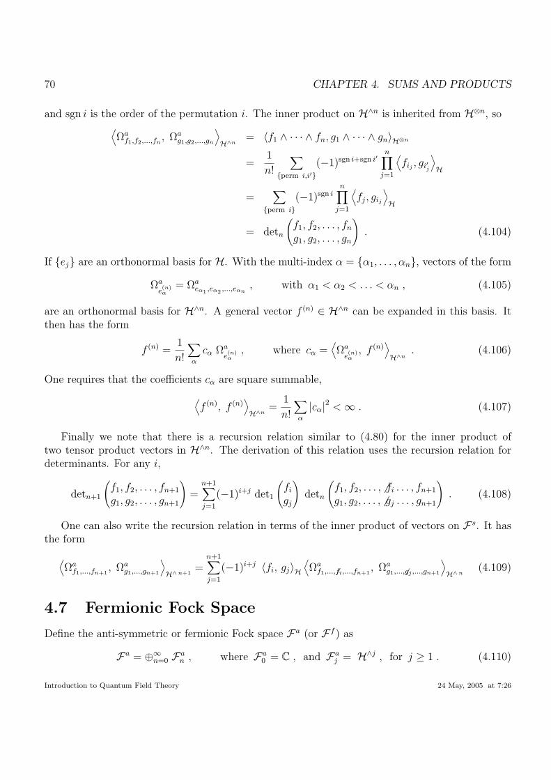
70 CHAPTER 4. SUMS AND PRODUCTS
and sgn i is the order of the permutation i. The inner product on H∧n is inherited from H⊗n, so⟨Ωa
f1,f2,...,fn, Ωa
g1,g2,...,gn
⟩H∧n
= 〈f1 ∧ · · · ∧ fn, g1 ∧ · · · ∧ gn〉H⊗n
=1
n!
∑perm i,i′
(−1)sgn i+sgn i′n∏
j=1
⟨fij , gi′j
⟩H
=∑
perm i(−1)sgn i
n∏j=1
⟨fj, gij
⟩H
= detn
(f1, f2, . . . , fn
g1, g2, . . . , gn
). (4.104)
If ej are an orthonormal basis for H. With the multi-index α = α1, . . . , αn, vectors of the form
Ωa
e(n)α
= Ωaeα1 ,eα2 ,...,eαn
, with α1 < α2 < . . . < αn , (4.105)
are an orthonormal basis for H∧n. A general vector f (n) ∈ H∧n can be expanded in this basis. Itthen has the form
f (n) =1
n!
∑α
cα Ωa
e(n)α, where cα =
⟨Ωa
e(n)α, f (n)
⟩H∧n
. (4.106)
One requires that the coefficients cα are square summable,⟨f (n), f (n)
⟩H∧n
=1
n!
∑α
|cα|2 <∞ . (4.107)
Finally we note that there is a recursion relation similar to (4.80) for the inner product oftwo tensor product vectors in H∧n. The derivation of this relation uses the recursion relation fordeterminants. For any i,
detn+1
(f1, f2, . . . , fn+1
g1, g2, . . . , gn+1
)=
n+1∑j=1
(−1)i+j det1
(fi
gj
)detn
(f1, f2, . . . , 6 fi . . . , fn+1
g1, g2, . . . , 6 gj . . . , gn+1
). (4.108)
One can also write the recursion relation in terms of the inner product of vectors on F s. It hasthe form
⟨Ωa
f1,...,fn+1, Ωa
g1,...,gn+1
⟩H∧n+1
=n+1∑j=1
(−1)i+j 〈fi, gj〉H⟨Ωa
f1,...,6fi,...,fn+1, Ωa
g1,...,6gj ,...,gn+1
⟩H∧n
(4.109)
4.7 Fermionic Fock Space
Define the anti-symmetric or fermionic Fock space Fa (or Ff ) as
Fa = ⊕∞n=0 Fa
n , where Fa0 = C , and Fa
j = H∧j , for j ≥ 1 . (4.110)
Introduction to Quantum Field Theory 24 May, 2005 at 7:26
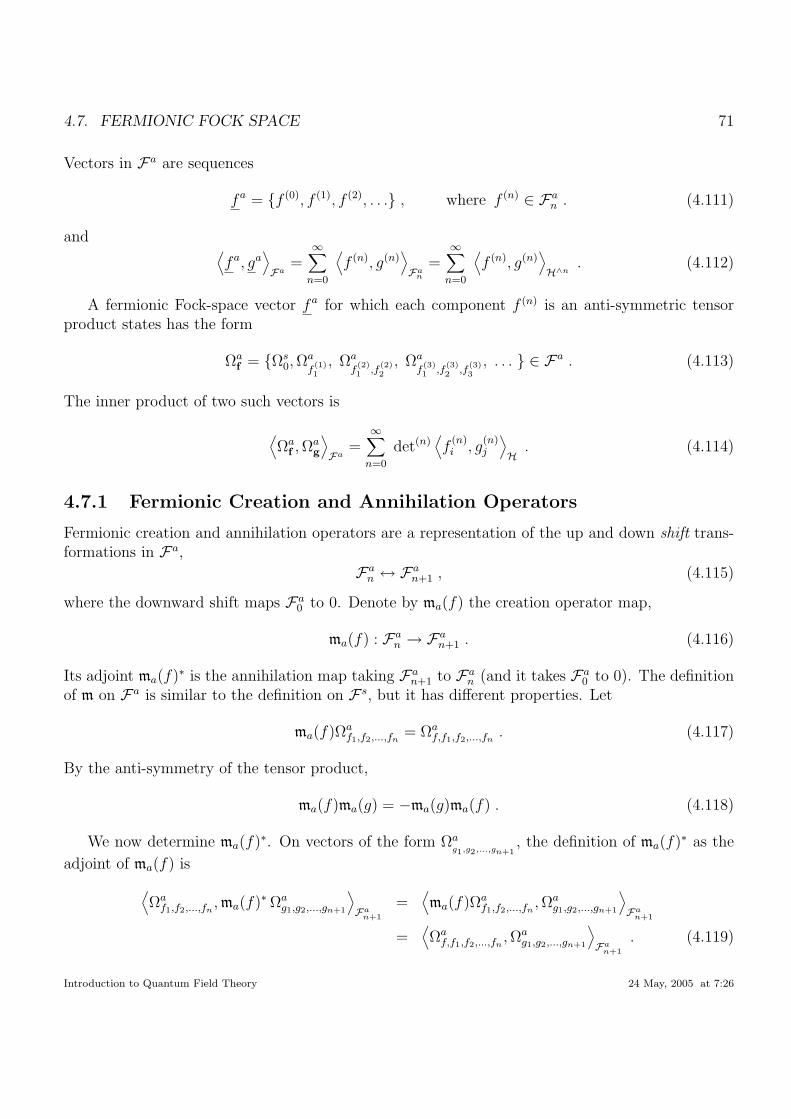
4.7. FERMIONIC FOCK SPACE 71
Vectors in Fa are sequences
fa = f (0), f (1), f (2), . . . , where f (n) ∈ Fan . (4.111)
and ⟨fa, ga
⟩Fa
=∞∑
n=0
⟨f (n), g(n)
⟩Fa
n
=∞∑
n=0
⟨f (n), g(n)
⟩H∧n
. (4.112)
A fermionic Fock-space vector fa for which each component f (n) is an anti-symmetric tensorproduct states has the form
Ωaf = Ωs
0,Ωa
f(1)1
, Ωa
f(2)1 ,f
(2)2
, Ωa
f(3)1 ,f
(3)2 ,f
(3)3
, . . . ∈ Fa . (4.113)
The inner product of two such vectors is
⟨Ωa
f ,Ωag
⟩Fa
=∞∑
n=0
det(n)⟨f
(n)i , g
(n)j
⟩H. (4.114)
4.7.1 Fermionic Creation and Annihilation Operators
Fermionic creation and annihilation operators are a representation of the up and down shift trans-formations in Fa,
Fan ↔ Fa
n+1 , (4.115)
where the downward shift maps Fa0 to 0. Denote by ma(f) the creation operator map,
ma(f) : Fan → Fa
n+1 . (4.116)
Its adjoint ma(f)∗ is the annihilation map taking Fan+1 to Fa
n (and it takes Fa0 to 0). The definition
of m on Fa is similar to the definition on F s, but it has different properties. Let
ma(f)Ωaf1,f2,...,fn
= Ωaf,f1,f2,...,fn
. (4.117)
By the anti-symmetry of the tensor product,
ma(f)ma(g) = −ma(g)ma(f) . (4.118)
We now determine ma(f)∗. On vectors of the form Ωag1,g2,...,gn+1
, the definition of ma(f)∗ as the
adjoint of ma(f) is⟨Ωa
f1,f2,...,fn,ma(f)∗ Ωa
g1,g2,...,gn+1
⟩Fa
n+1
=⟨ma(f)Ωa
f1,f2,...,fn,Ωa
g1,g2,...,gn+1
⟩Fa
n+1
=⟨Ωa
f,f1,f2,...,fn,Ωa
g1,g2,...,gn+1
⟩Fa
n+1
. (4.119)
Introduction to Quantum Field Theory 24 May, 2005 at 7:26
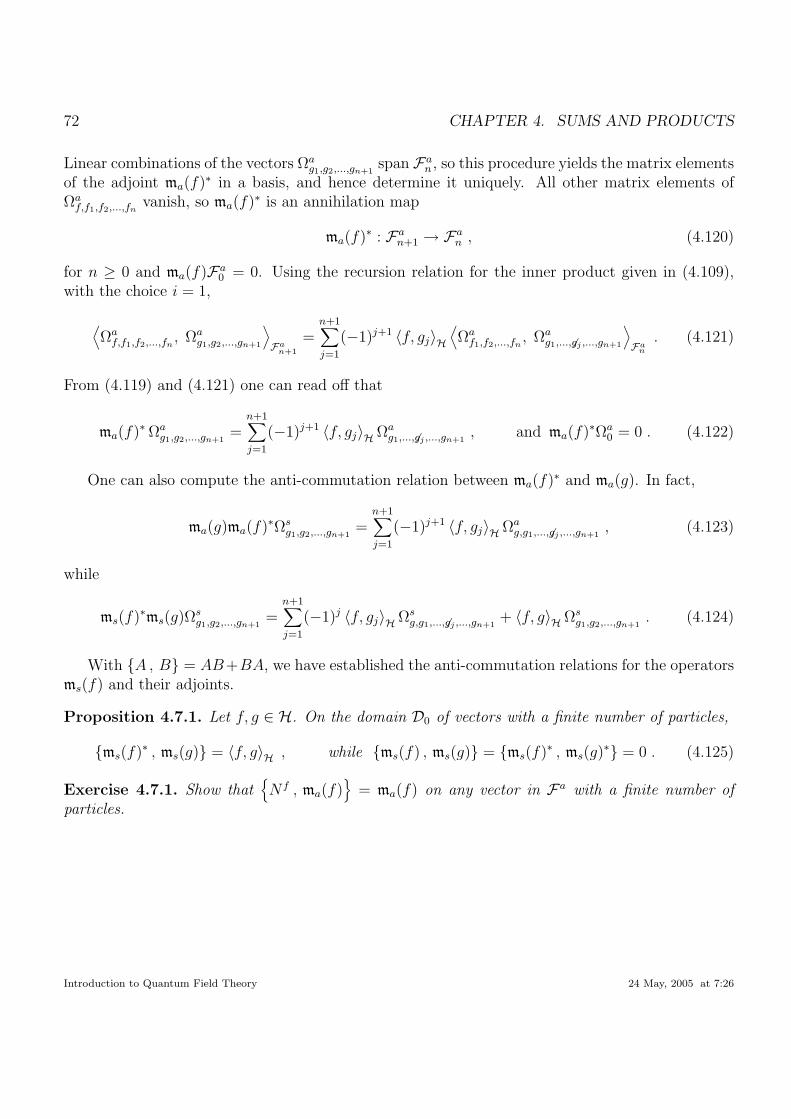
72 CHAPTER 4. SUMS AND PRODUCTS
Linear combinations of the vectors Ωag1,g2,...,gn+1
span Fan , so this procedure yields the matrix elements
of the adjoint ma(f)∗ in a basis, and hence determine it uniquely. All other matrix elements ofΩa
f,f1,f2,...,fnvanish, so ma(f)∗ is an annihilation map
ma(f)∗ : Fan+1 → Fa
n , (4.120)
for n ≥ 0 and ma(f)Fa0 = 0. Using the recursion relation for the inner product given in (4.109),
with the choice i = 1,
⟨Ωa
f,f1,f2,...,fn, Ωa
g1,g2,...,gn+1
⟩Fa
n+1
=n+1∑j=1
(−1)j+1 〈f, gj〉H⟨Ωa
f1,f2,...,fn, Ωa
g1,...,6gj ,...,gn+1
⟩Fa
n
. (4.121)
From (4.119) and (4.121) one can read off that
ma(f)∗ Ωag1,g2,...,gn+1
=n+1∑j=1
(−1)j+1 〈f, gj〉H Ωag1,...,6gj ,...,gn+1
, and ma(f)∗Ωa0 = 0 . (4.122)
One can also compute the anti-commutation relation between ma(f)∗ and ma(g). In fact,
ma(g)ma(f)∗Ωsg1,g2,...,gn+1
=n+1∑j=1
(−1)j+1 〈f, gj〉H Ωag,g1,...,6gj ,...,gn+1
, (4.123)
while
ms(f)∗ms(g)Ωsg1,g2,...,gn+1
=n+1∑j=1
(−1)j 〈f, gj〉H Ωsg,g1,...,6gj ,...,gn+1
+ 〈f, g〉H Ωsg1,g2,...,gn+1
. (4.124)
With A , B = AB+BA, we have established the anti-commutation relations for the operatorsms(f) and their adjoints.
Proposition 4.7.1. Let f, g ∈ H. On the domain D0 of vectors with a finite number of particles,
ms(f)∗ , ms(g) = 〈f, g〉H , while ms(f) , ms(g) = ms(f)∗ , ms(g)∗ = 0 . (4.125)
Exercise 4.7.1. Show thatN f , ma(f)
= ma(f) on any vector in Fa with a finite number of
particles.
Introduction to Quantum Field Theory 24 May, 2005 at 7:26
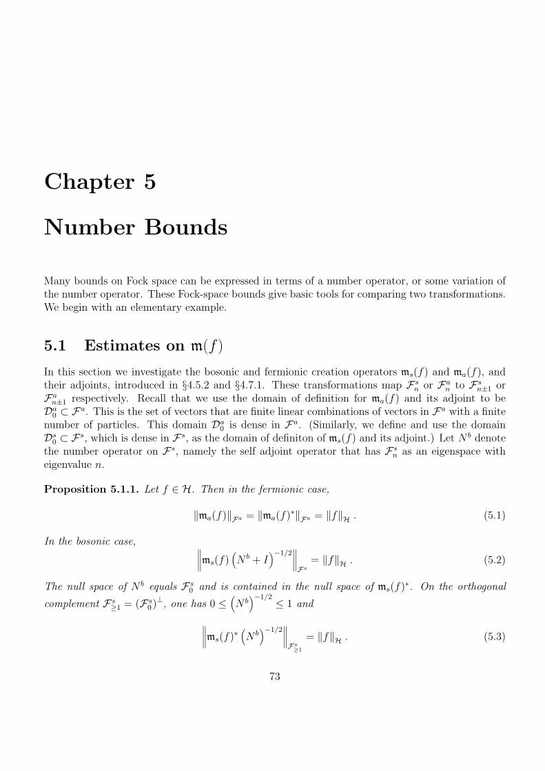
Chapter 5
Number Bounds
Many bounds on Fock space can be expressed in terms of a number operator, or some variation ofthe number operator. These Fock-space bounds give basic tools for comparing two transformations.We begin with an elementary example.
5.1 Estimates on m(f )
In this section we investigate the bosonic and fermionic creation operators ms(f) and ma(f), andtheir adjoints, introduced in §4.5.2 and §4.7.1. These transformations map F s
n or Fan to F s
n±1 orFa
n±1 respectively. Recall that we use the domain of definition for ma(f) and its adjoint to beDa
0 ⊂ Fa. This is the set of vectors that are finite linear combinations of vectors in Fa with a finitenumber of particles. This domain Da
0 is dense in Fa. (Similarly, we define and use the domainDs
0 ⊂ F s, which is dense in F s, as the domain of definiton of ms(f) and its adjoint.) Let N b denotethe number operator on F s, namely the self adjoint operator that has F s
n as an eigenspace witheigenvalue n.
Proposition 5.1.1. Let f ∈ H. Then in the fermionic case,
‖ma(f)‖Fa = ‖ma(f)∗‖Fa = ‖f‖H . (5.1)
In the bosonic case, ∥∥∥∥ms(f)(N b + I
)−1/2∥∥∥∥Fs
= ‖f‖H . (5.2)
The null space of N b equals F s0 and is contained in the null space of ms(f)∗. On the orthogonal
complement F s≥1 = (F s
0 )⊥, one has 0 ≤(N b)−1/2
≤ 1 and
∥∥∥∥ms(f)∗(N b)−1/2
∥∥∥∥Fs≥1
= ‖f‖H . (5.3)
73
74 CHAPTER 5. NUMBER BOUNDS
Proof. The transformations ms(f) and ma(f) are linear in f , and vanish for f = 0, in which casethe claims hold. Thus without loss of generality assume f 6= 0, and by scaling assume ‖f‖H = 1.
In the fermionic case, consider the positive, self-adjoint operators Na(f) = ma(f)ma(f)∗ andNa(f) = ma(f)∗ma(f). The commutation relations (4.125) ensure for g = f that
Na(f) + Na(f) = I . (5.4)
Thus 0 ≤ Na(f) ≤ I, and similarly for Na(f). Also
ma(f)2 = (ma(f)∗)2 = 0 , (5.5)
which entails that both Na(f) and Na(f) are projections. As they sum to I, they cannot bothvanish. One checks the projection property for Na(f), for example, by writing
Na(f)2 = ma(f) ma(f) , ma(f)∗ma(f)∗ = ‖f‖2H ma(f)ma(f)∗ = Na(f) . (5.6)
As any linear transformation ma(f) on a Hilbert space and its adjoint have the same norm,
‖ma(f)∗‖Fa = ‖Na(f)‖1/2Fa = ‖ma(f)‖Fa = ‖Na(f)‖1/2
Fa . (5.7)
so both Na(f) and Na(f) have norm 1.In the bosonic case the commutation relation (4.97) in the case g = f of norm one take the form
ms(f)∗ms(f) = ms(f)ms(f)∗ + I = N s(f) + I . (5.8)
Again this allows us to diagonalize N s(f) = ms(f)ms(f)∗. Choose an orthonormal basis ej forH, with e1 = f , and let Ωs
f (n) = Ωs...,0,f (n),0,...
∈ F s ∩ F sn denote an element of the corresponding
orthonormal basis for F s obtained by choosing all possible n = 0, 1, . . . and all possible f (n) of theform (4.71). We show that these vectors are also eigenvectors for N s(f). The commutation relation(4.97) yields
[N s(f),ms(ej)] = δ1j ms(ej) , (5.9)
Thus any such vector Ωsf (n) of the form (4.71), and with i1 > 1, is a null vector for N s(f). Further-
more, the relation (5.9) shows that ms(f) acts on an eigenvector of N s(f) with eigenvalue λ, yieldsanother eigenvector of N s(f) with the eigenvalue raised to λ+ 1. We infer that an element Ωs
f (n) is
an eigenvector of N s(b) with eigenvalue δi11ni1 . Taken together with (5.8), we see observe that theΩs
f (n) also give a basis of eigenvectors for ms(f)∗ms(f). This completes the proof of the two claimedbounds.
Remark 5.1.2. For f 6= 0, one sometimes calls
Na(f) = ‖f‖−2H ma(f)ma(f)∗ , (5.10)
the fermion number operator for mode f . Likewise
N s(f) = ‖f‖−2H ms(f)ms(f)∗ , (5.11)
is called the boson number operator form mode f , and it has spectrum Z+.
Introduction to Quantum Field Theory 24 May, 2005 at 7:26
5.2. NICE VECTORS 75
5.2 Nice Vectors
We often need a suitable regular, dense subset of nice vectors D ⊂ F of Fock space to use as thebasis domain of definition of certain operators operators. Likewise we use D×D as the basis domainfor certain forms. We also use the domain D to carry out computations, such as the verification ofcommutation relations for the densities of the fields, to discover the symmetry generated by someself-adjoint transformation, etc. We then extend these relations by continuity to some larger domainby continuity or by other means.
In fact we introduce two such domains: a nice domain Db ⊂ F b = F s for bosons and also a nicedomain Df ⊂ Ff = Fa for fermions. Both spaces are defined in the same way. In each case, let Hdenote the one-particle space and let H0 ⊂ H denote a dense subspace of “nice” one-particle wavefunctions. We choose D to be vectors that are finite linear combinations of vectors in D0, wherevectors Ω ∈ D0 have the properties:
• Any Ω ∈ D0 has a finite number of non-zero n-particle components Ωn.
• Each Ωn is the tensor products of n-nice, one-particle wave functions in H0.
In the bosonic case, the wave functions are symmetric tensor products of one-particle wave functions;in the fermionic case the wave functions are anti-symmetric tensor products of one-particle wavefunctions.
5.3 The Weyl Algebra
Define the self-adjiont part of the bosonic creation operator ms(f) of (4.91) as
X(f) = ms(f) + ms(f)∗ , (5.12)
with the domain Db ⊂ F b. This operator is a generator in the Weyl algebra as follows. Note also,
X(if) = i (ms(f)−ms(f)∗) . (5.13)
Furthermore
[X(f), X(g)] = (f, g)H − (g, f)H = 2i= (f, g)H . (5.14)
Proposition 5.3.1. For f ∈ H, the transformation X(f) is essentially self adjoint on Db. Wedenote the closure also by X(f). The unitary Weyl operators W (f) = eiX(f) satisfy
W (f)W (g) = ei=〈f,g〉H W (f + g) , (5.15)
which applied twice yields,
W (f)W (g) = e2i=〈f,g〉H W (g)W (f) . (5.16)
Introduction to Quantum Field Theory 24 May, 2005 at 7:26
76 CHAPTER 5. NUMBER BOUNDS
Remark 5.3.2. Two Weyl operators W (f) and W (g) commute, if and only if
= 〈f, g〉H ∈ πZ . (5.17)
Proof. Let Ω ∈ D0 be a vector with n0 or fewer particles. Expand X(f)j into a linear combinationof 2j monomials of the form Y (f) = ms(f)#1ms(f)#2 · · ·ms(f)#j , where each # denotes the choiceof either ms(f) or ms(f)∗, with j = j1 + j2 specifying j1 ≥ 0 choices of ms(f) and j2 ≥ 0 choices ofms(f)∗. One verifies on each n particle eigenspace of N b that
ms(f)(N b + 1
)−1/2=(N b)−1/2
ms(f) . (5.18)
It follows that
‖Y (f)Ω‖F =∥∥∥∥Y (f)
(N b + j + 1
)−j/2 (N b + j + 1
)j/2Ω∥∥∥∥Fb
≤∥∥∥∥Y (f)
(N b + j + 1
)−j/2∥∥∥∥Fb
∥∥∥∥(N b + j + 1)j/2
Ω∥∥∥∥Fb
≤ (n0 + j + 1)j/2∥∥∥∥Y (f)
(N b + j + 1
)−j/2∥∥∥∥Fb‖Ω‖Fb . (5.19)
But (5.18) combined with Proposition 5.1.1 means that∥∥∥∥Y (f)(N b + j + 1
)−j/2∥∥∥∥Fb≤ ‖f‖j
H . (5.20)
Therefore, ∥∥∥X(f)jΩ∥∥∥Fb≤ 2j (n0 + j + 1)j/2 ‖f‖j
H‖Ω‖Fb , (5.21)
from which we infer that the power series
∞∑j=0
λj
j!
∥∥∥X(f)jΩ∥∥∥Fb, (5.22)
converges to a function of an entire function of λ‖f‖H of exponential order 2. Thus X(f) has adense set of analytic vectors, and its closure is self-adjoint.
Next consider the self-adjoint operator
G(λ) = W (λf)X(g)W (−λf) , (5.23)
with domain D. On this domain, G(λ) also has power series in λ with infinite radius of convergence.As all derivatives at the origin of order 2 or more vanish,
G(λ) = X(g) + 2iλ= 〈f, g〉 . (5.24)
This identity extends by continuity to the domain of X(g).
Introduction to Quantum Field Theory 24 May, 2005 at 7:26
5.4. SOME ADDITIONAL PROPERTIES WHEN H = H−1/2(RD−1) 77
Next with Ω ∈ D0 consider the entire function
F (λ) = e−iλ2=〈f,g〉 W (−λ(f + g))W (λf)W (λg)Ω . (5.25)
Note F (0) = Ω. Use (5.24) to obtain
dF (λ)
dλ= e−iλ2=〈f,g〉 W (−λ(f + g)) (X(−g)− 2iλ= 〈f, g〉)W (λf)W (λg)Ω
+e−iλ2=〈f,g〉 W (−λ(f + g))W (λf)X(g)W (−λf)W (λf)W (λg)Ω = 0 . (5.26)
Therefore, F (λ) = Ω, which yields the desired identity (5.15) and completes the proof.
5.4 Some Additional Properties when H = H−1/2(Rd−1)
In this section we assume that H is a function space. In particular for simplicity we choose H =H−1/2(Rd−1). The important feature is that H includes a dense set of nice vectors, and we choosethese vectors to be either
d1 = S(Rd−1) , or d0 = e−ω2
d1 . (5.27)
Introduction to Quantum Field Theory 24 May, 2005 at 7:26

78 CHAPTER 5. NUMBER BOUNDS
Introduction to Quantum Field Theory 24 May, 2005 at 7:26
Part III
Quantum Fields
79

81
Quantum Fields describe an arbitrary number of particles. Thus the Hilbert space on whichthey live has a more complicated structure than the Hilbert spaces in Proposition I called We beginwith the construction of a Fock space H, the natural Hilbert space appropriate for a free (linear)quantum field. For simplicity we begin with a field that describes a single type of scalar (spin zero)particle with mass m > 0. One generally begins the study of non-linear or interacting field byperturbing such a linear field.
We take an appropriate Hilbert space H1 for a single particle. This space will be given an uni-tary, irreducible, positive energy representation U(Λ, a) of the Poincare group (the inhomogeneousLorentz group). Such a representation is characterized by the spin and mass, so we have used upour freedom of choice. The full Fock space is the symmetric tensor product exponential of the one-particle space, H = exp⊗s
H1. The unitary representation of the Poincare group on H1 determinesa corresponding unitary representation U(Λ, a). This representation is highly reducible, and hasthe interpretation of acting on each of the individual particles.
We begin with a discussion of tensor products that make up the Hilbert space to describe anarbitrary number of particles. This is the space of states for the free field.
Introduction to Quantum Field Theory 24 May, 2005 at 7:26

82
Introduction to Quantum Field Theory 24 May, 2005 at 7:26
Chapter 6
The Free Bosonic Field
In this chapter we define the mass-m, scalar, free quantum field ϕ(~x, t), acting on Minkowski space-time Rd−1 × R. This field is an operator-valued distribution that satisfies the linear equation ofmotion (
+m2)ϕ(~x, t) = 0 , (6.1)
along with the canonical constraints on the initial data
ϕ(~x) = ϕ(~x, 0) , and π(~x) =
(∂ϕ
∂t
)(~x, 0) , (6.2)
that satisfy
[π(~x), ϕ(~x′)] = −iδ(~x− ~x′), and [ϕ(~x), ϕ(~x′)] = 0 = [π(~x), π(~x′)] . (6.3)
6.1 The Local Field
A local field ϕ(x) = ϕ(~x, t) arises from giving the time-zero field ϕ(~x) the time-dependence generatedby a local Hamiltonian H,
ϕ(x) = eitHϕ(~x)e−itH . (6.4)
A local Hamiltonian is one which propagates the field with finite speed, so that ϕ(x) and ϕ(x′)commute when x − x′ is a space-like Minkowski vector. If H = H0 is the free field Hamiltonian,then ϕ(x) is hte free field. We first describe the space of state, introduce the initial field ϕ(~x), andthen define the time-dependent free field ϕ(~x, t).
6.1.1 The Hilbert Space
The Hilbert space of the massive, free scalar field is the bosonic Fock space F b over the one particlespace H. In the notation of Chapter 4,
F b = F s = exp⊗sH . (6.5)
83
84 CHAPTER 6. THE FREE BOSONIC FIELD
A single-component field has the one-particle space H = H−1/2(Rd−1), namely the Sobolev spaceintroduced (??), with inner product
〈f, g〉H−1/2(Rs) =⟨f, (2ω)−1 g
⟩L2(Rs)
. (6.6)
Here ω = (−∇2 +m2)1/2
is the relativistic energy for a mass-m particle. The action of ω on F b isgiven by the free-field Hamiltonian H0. In terms of the operator Γs defined in (4.60)–(4.61),
H0 = − d
dtΓ(e−tω)
∣∣∣∣∣t=0
. (6.7)
The operator H0 acts on states Ωsf (n) ∈ F s
n as
n factors︷ ︸︸ ︷ω ⊗ I ⊗ · · · ⊗ I + · · ·+ I ⊗ · · · ⊗ I ⊗ ω︸ ︷︷ ︸
n terms
. (6.8)
Exercise 6.1.1. Show that the creation operators ms(f) of (4.91) and their adjoints satisfy
[H0,ms(f)] = ms(ωf) , and [H0,ms(f)∗] = −ms(ωf)∗ , (6.9)
or in unitary form
eitH0ms(f)e−itH0 = ms(eitωf) , and eitH0ms(f)∗e−itH0 = ms(e
itωf)∗ . (6.10)
The unitary representation U(Λ, a) of the Poincare group on F1 gives rise to a unitary repre-sentation of the Poincare group on F equal to
Γs(U(Λ, a)) . (6.11)
Thus we obtain a unitary representation of the Poincare group on F b. By definition, This groupleaves the vector f = 1, 0, 0, 0, . . . invariant, and one calls this the no-particle vector the vacuum-vector
Ωs0 = 1, 0, 0, 0, . . . . (6.12)
The vacuum is an eigenvector of each generator of the Poincare group with eigenvalue zero. Thesegenerators are identified with energy, momentum, angular momentum, and infinitesimal boosts.Thus
H0Ωs0 = PjΩ
s0 = LijΩ
s0 = MijΩ
s0 = 0 . (6.13)
Introduction to Quantum Field Theory 24 May, 2005 at 7:26
6.1. THE LOCAL FIELD 85
6.1.2 Time-Zero Fields
We continue with the choice of 〈·, ·〉H as the space (6.49) of generalized functions H−1/2. Then anyf ∈ H can be decomposed into real and imaginary parts,
f = fr + ifi , with fr, fi real . (6.14)
Let us defineH−1/2 real(Rs) = f : f ∈ H−1/2(Rs) , and f = fr . (6.15)
The operator ω is real. This means that ω (as well as a real function of ω) transforms real functionf to real functions f , so if f ∈ D(ω),
ωf = ωfr + ωf1 . (6.16)
The self-adjoint part of the creation operator ms(f) for real and purely imaginary functionsf ∈ H play a special role. Recall we already introduced the self adjoint part of ms(f) for generalf ∈ H in (5.12); we called X(f) the generator of a unitary Weyl operator W (f) = eiX(f).
Definition 6.1.1. The time-zero boson field ϕ is
ϕ(f) = X(f) = ms(f) + ms(f)∗ , in case f ∈ H−1/2 real(Rs) . (6.17)
The canonically conjugate time-zero field is π, given as
π(f) = X(iωf) = i (ms(ωf)−ms(ωf)∗) , in case ωf ∈ H−1/2 real(Rs) . (6.18)
With these choices, the fundamental commutation relation (5.14) for real f, g take their standardform.
Proposition 6.1.2. The canonical fields satisfy
[π(f), ϕ(g)] = −i 〈f, g〉L2(Rs) , (6.19)
and the Weyl relation (5.16) becomes
eiπ(f) eiϕ(g) = ei〈f,g〉L2(Rs) eiϕ(g) eiπ(f) . (6.20)
Proof. These relations follow from
[π(f), ϕ(g)] = 2i= 〈iωf, g〉H−1/2(Rs) = −i 〈f, 2ωg〉H−1/2(Rs) = −i 〈f, g〉L2(Rs) , (6.21)
and the Weyl relation (5.16). We can extend ϕ(f) and π(f) in an linear manner to all functionsf = fr + ifi in H−1/2(Rs) or H−3/2(Rs) respectively. In this way,
ϕ(f) = ms(f) + ms(f)∗
π(f) = i(ms(ωf)−ms(ωf)∗
). (6.22)
Introduction to Quantum Field Theory 24 May, 2005 at 7:26
86 CHAPTER 6. THE FREE BOSONIC FIELD
If one wanted, one could express this inelegantly in terms of the X(f)’s. For example,
ϕ(f) =1
2
(X(f) +X(f)− iX(if) + iX(if)
). (6.23)
Once these fields have been defined, one can extend them (linearly) to complex test functionsf . Thus with f decomposed as in (6.14) or (6.17), let
ϕ(f) = ϕ(fr) + iϕ(fi) , and π(f) = π(fr) + iπ(fi) , (6.24)
6.2 The Free Field
The initial value for the field ϕ and its canonically conjugate field π do not determine the timeevolution of the field. That is given by the Hamiltonian. For the free field, we already introducedthe Hamiltonian H0. We use the Hamiltonian to define the time translation. For the free field, takea real test function f and define
ϕ(f, t) = eitH0
(ms(f) + ms(f)
∗)e−itH0
= ms(eitωf) + ms(eitωf)∗ . (6.25)
ϕ(f)Ωs0 = Ωs
f . (6.26)
One recovers the standard creation operators by introducing
a∗(f) = ms((2ω)1/2f) , and a(f) = a(f)∗ = ms(f)∗ . (6.27)
As a consequence of the commutation relations (4.97) for the operators ms and m∗s, one sees that
the transformations a, a∗ satisfy
[a(f), a∗(g)] =⟨f, g⟩
L2(Rs). (6.28)
One can also write (6.9) as[H0, a
∗(f)] = a∗(ωf) . (6.29)
Thus the time-zero field can be written in its usual form,
ϕ(f) =1√2
(a∗(ω−1/2f) + a(ω−1/2f)
), (6.30)
and the time-dependent field is
ϕ(f, t) =1√2
(a∗(eitωω−1/2f) + a(e−itωω−1/2f)
). (6.31)
Introduction to Quantum Field Theory 24 May, 2005 at 7:26
6.2. THE FREE FIELD 87
This field satisfies the equation of motion. One has
∂2
∂t2ϕ(f, t) = −a∗(eitω(2ω)−1/2ω2f)− a(e−itω(2ω)−1/2ω2f) (6.32)
As ω2 = −∇2 + m2, one has the distribution equation (6.1) ω2 = −∇2 + m2. Furthermore, theinitial data for the time derivative is determined by differentiating the representation (6.31) anddefining
π(f) =∂ϕ(f, t)
∂t
∣∣∣∣∣t=0
=i√2
(a∗(ω1/2f)− a(ω1/2f)
). (6.33)
The commutation relations at fixed time are
[π(f), ϕ(g)] = −i⟨f, g⟩
L2(Rs), and [ϕ(f), ϕ(g)] = 0 = [π(f), π(g)] . (6.34)
6.2.1 Fields at a Point
We express a(f) as a density
a(f) =∫
Rsa(~x)f(~x)d~x , and a∗(f) =
∫Rsa∗(~x)f(~x)d~x . (6.35)
The densities for a, a∗ are forms, not operators, which we deal with shortly in §6.5. They satisfy
[a(~x), a∗(~y)] = δ(~x− ~y) , and [a(~x), a(~y)] = [a∗(~x), a∗(~y)] = 0 . (6.36)
Exercise 6.2.1. Show that the bosonic number operator N b and the bosonic Hamiltonian H0 asdefined above agree with the ususal definitions,
N b =∫
Rsa∗(~x)a(~x)d~x , and H0 =
∫Rsa∗(~x)ω a(~x)d~x . (6.37)
With these densities,
ϕ(~x, t) = eitH0ϕ(~x)e−itH0
=1√2ω
(eitωa∗(~x) + e−itωa(~x)
). (6.38)
6.2.2 Momentum Space Representation
We have a corresponding Fourier representation. Define
a(~x) =1
(2π)s/2
∫Rsei~k·~xa(~k)d~k , or equivalently a(~k) =
1
(2π)s/2
∫Rse−i~k·~xa(~x)d~x . (6.39)
Introduction to Quantum Field Theory 24 May, 2005 at 7:26
88 CHAPTER 6. THE FREE BOSONIC FIELD
Then
a∗(~x) =1
(2π)s/2
∫Rse−i~k·~xa∗(~k)d~k , or a∗(~k) =
1
(2π)s/2
∫Rsei~k·~xa∗(~x)d~x . (6.40)
As a consequence of (6.36), these forms satisfy[a(~k), a∗(~k′)
]= δ(~k − ~k′) , and
[a(~k), a(~k′)
]=[a∗(~k), a∗(~k′)
]= 0 . (6.41)
In the momentum representation, ω acts as the multiplication operator ω(~k). Then the representa-tion for the field (6.38) takes the usual form
ϕ(~x, t) =1
(2π)s/2
∫Rs
1√2ω(~k)
(eitω(~k)−i~k·~xa∗(~k) + e−itω(~k)+i~k·~xa(~k)
)d~k . (6.42)
6.2.3 Commutation Relation
The commutation relation for the free field is easy to commute, as the time dependence allows oneto express the field as a linear combination of creation and annihilation operators, see (6.42) thatsatisfy the canonical commutation relations. Thus
[ϕ(~x, t), ϕ~x′, t′] = 〈Ω0, ϕ(~x, t)ϕ(~x′, t′)Ω0〉 − 〈Ω0, ϕ(~x′, t′)ϕ(~x, t)Ω0〉= W (x− x′)−W (x′ − x) = ∆(x− x′) , (6.43)
where W (x− x′) is the Poincare-invariant generalized function
W (x− x′) =1
(2π)s
∫kd>0
e−ik(x−x′)δ(k2 −m2)dk . (6.44)
Note ∆(x) and W (x) are are both Lorentz-invariant generalized functions that are solutions to theKlein-Gordon equation. (Do not confuse this ∆ with the Laplace operator.) The solution W (x)has the initial data
W (~x, 0) = G(~x) , and
(∂W
∂t
)(~x, 0) = − i
2δ(~x) . (6.45)
where G(~x) is the Green’s function of (2ω)−1(~x) introduced in (2.53). The solution ∆(x) has theinitial data
∆(~x, 0) = 0 , and
(∂∆
∂t
)(~x, 0) = −iδ(~x) . (6.46)
If x− x′ is a space-like vector, i.e. (x− x′)2 < 0, then there is a Lorentz transformation Λ suchthat Λ(x− x′) = x′ − x. Clearly W (x) = W (Λx) is invariant invariant (in the sense of generalizedfunctions) so
[ϕ(~x, t), ϕ~x′, t′] = ∆(x− x′) = 0 , for (x− x′)2< 0 . (6.47)
Introduction to Quantum Field Theory 24 May, 2005 at 7:26
6.3. IMAGINARY TIME FIELDS 89
6.3 Imaginary Time Fields
The imaginary time field is defined by
ϕI(~x, t) = ϕ(~x, it) = e−tH0ϕ(~x)etH0 . (6.48)
6.4 Compact Space
On the other hand, in case we use the compactified space equal to a torus Ts, then we choose
H = H−1/2(Ts) , (6.49)
where the one-particle inner product is
〈f, g〉H−1/2(Ts) =⟨(2ωT )−1/2 f, (2ωT)−1/2 g
⟩L2(Rs)
. (6.50)
Here
ωT =(−∇2
T +m2)1/2
. (6.51)
Likewise, if we work on a different one-particle space such as a lattice space, a section of a Riemannsurface, etc., we take the appropriate definition of H.
6.5 Forms and Number Bounds
In case of ordinary quantum field theory defined on Euclidean space Rs, we take H0 to be theSchwartz space
H0 = S(Rs) . (6.52)
Then transformations such as (positive or negative fractional) powers of ω, or e−tω with t ≥ 0, mapH0 to H0. Such transformations are determined uniquely as self-adjiont transformations on H bydefining them on this domain H0.
6.6 Poincare Invariance
6.7 Locality
6.8 Wightman Functions
6.9 Reeh-Schlieder Property
Introduction to Quantum Field Theory 24 May, 2005 at 7:26

90 CHAPTER 6. THE FREE BOSONIC FIELD
Introduction to Quantum Field Theory 24 May, 2005 at 7:26
Chapter 7
The Fundamental Bound for Fields
Perhaps the most fundamental operator in a field theory is the Hamiltonian H, which we assume isself-adjoint and positive. Stability of the Hamiltonian 0 ≤ H is central to many aspects of physics.Having a Hamiltonian, we turn to the field itself. The property of the time-zero field ϕ(g) thatserves as a fundamental starting point is the key bound, comparing the the field ϕ(g) with theHamiltonian H. The key bound provides the input to a robust machine from which one can derivemany desired properties of quantum field operators.
The key bound is not a consequence of the Wightman axioms for quantum field theory, nor ofthe Osterwalder-Schrader axioms for Euclidean Green’s functions. The key bound is an additionalproperty that we desire as a starting point for our quantum fields. It is a property that we returnto in later chapters where we develop methods to ensure that the key bound holds.
In this chapter, we highlight why we want to establish the key bound, by showing that it ensuresa number of fundamental properties of the fields. For example, the key bound lets us pass fromfields that are forms to fields that are operators on Hilbert space. It also ensures that the fieldoperators are self-adjoint. The key bound ensures also that expectation values of all products offield operators exist. In addition, the key bound entails that the fields are local in the sense that ifthe commutator of two fields [ϕ(f), ϕ(g)] = 0, then quantum mechanical observables depending onthe field ϕ(f) commute with those depending on the field ϕ(g).
We introduce the time-zero field as a form.1 This means that we initially study matrix elementsof the field (or equivalently expectation values of the field) in states Ω that are “smooth vectors”for the Hamiltonian H. This means that Ω is in the domain of arbitrary powers Hn of the theHamiltonian H, which we write Ω ∈ C∞(H).
1See §8.5 for the a full definition of forms, as well as for a discussion of certain properties of forms.
91
92 CHAPTER 7. THE FUNDAMENTAL BOUND FOR FIELDS
7.1 The Fundamental Bound
We assume that the time-zero field ϕ(g) is a form with domain C∞(H)× C∞(H). The key boundsays:
±ϕ(g) ≤ H + I , (7.1)
for all real g ∈ C∞0 (Rs) for which ‖g‖K ≤ 1. In more detail, g is a test function g(~x) with
~x ∈ Rs = Rd−1. The norm ‖ · ‖K is a norm that is bounded by some finite linear combination ofSchwartz space norms on S(Rs).2 Define the normed space K as the completion of the set S(Rs)in the K-norm. As the field is a linear function of g, so once we have shown that it is true, we cansubstitute g/‖g‖K for g. Thus the key bound (7.1) is also equivalent to the bound,
±ϕ(g) ≤ ‖g‖K (H + I) , (7.2)
for all real g ∈ C∞0 (Rs).
The key bound is equivalent to a stability bound for perturbations of H, namely
0 ≤ H + I ± ϕ(g) , (7.3)
for all real g ∈ C∞0 for which ‖g‖K ≤ 1.
Example. The free time-zero, mass-m field and its Hamiltonian H = H0 provide a useful guide.One can find the exact lower bound of H0 + ϕ(g), namely
0 ≤ H0 + ϕ(g) +1
2
∥∥∥ω−1g∥∥∥2
L2(Rs), (7.4)
where ω = (−∇2 +m2)1/2. Thus in the case of the free field one can take the norm ‖ · ‖K to be
‖g‖K =1√2
∥∥∥ω−1g∥∥∥
L2(Rs), (7.5)
and K the corresponding Sobolev space H−1(Rs). With our choice of normalization, ϕ(g) satisfiesthe bound (7.1) for ‖g‖K ≤ 1.
In the particular case of spatial dimension s = 1, the Dirac measure δx ∈ K. Thus one canchoose g to be a real multiple λ of δx, in which case the time-zero free field ϕ(x) satisfies the keybound
±λϕ(x) ≤ H0 + I , as long as λ2 ≤ 4m (when s = 1) . (7.6)
2For example, as explained in §9.2 one can define the Schwartz space S(Rs) using the increasing family of norms‖g‖n = ‖hng ‖L2(Rs), with h is the Hamiltonian of a homogeneous, unit-frequency harmonic oscillator on Rs. Inother words, take
h =12(−∆ + x2 − s
),
where ∆ denotes the Laplace operator on Rs, and where x ∈ Rs. In this case, S(Rs) = C∞(h), and we assume thatthere exists some n for which ‖g‖K ≤ ‖g‖n. Then every function g ∈ S(Rs) has finite norm ‖g‖K.
Introduction to Quantum Field Theory 24 May, 2005 at 7:26
7.1. THE FUNDAMENTAL BOUND 93
7.1.1 The Fundamental Bound and Field Operators
The space-time field ϕ(f) is
ϕ(f) =∫eitHϕ(~x)e−itHf(~x, t)dx , for f ∈ C∞
0 (Rd) , with Rd = Rs+1 . (7.7)
Clearly our assumption that the time-zero field ϕ(g) is a form on the domain C∞(H) × C∞(H),ensures that the space-time field ϕ(f) is also such a form. In fact C∞(H) is invariant under theunitary group e−itH . Therefore define the sharp time field ϕ(g(t)) for the test function g(t) equal to
g(t)(~x) = f(~x, t) . (7.8)
This field is a form on the domain C∞(H)×C∞(H), and the resulting form is a C∞ function of t.One can integrate this form over t to obtain the space-time field ϕ(f) =
∫ϕ(g(t)) dt.
Define a norm M(f) by
M(f) =∫ ∥∥∥g(t)
∥∥∥Kdt =
∫‖f(·, t)‖K dt . (7.9)
Then for real f the space-time field obeys the primitive bound
±ϕ(f) ≤M(f) (H + I) . (7.10)
The fundamental bound (7.1) allows us to pass from the form ϕ(f) with domain C∞(H)×C∞(H)to an operator ϕ(f) with the domain D(H). The requirement that ϕ(f) determine an operatorrequires a slightly more restrictive norm on f that includes one time derivative ∂tf = ∂f/∂t. Definethe norm
|||f ||| = M(f) +M(∂tf) . (7.11)
In the case of a product test function f = g ⊗ h, namely f(x) = g(~x)h(t) with f ′ = df/dt, one has
|||g ⊗ h||| = ‖g‖K(‖f‖L1(R) + ‖f ′‖L1(R)
). (7.12)
Theorem 7.1.1 (Field Operators). Assume that the time-zero field ϕ(g) is a form on the domainC∞(H) × C∞(H), and that ϕ(g) satisfies the key bound (7.1). Consider the space-time field ϕ(f)as the form defined in (7.7). Then all the following hold:
i. Field Operators Exist. Let f ∈ C∞0 . The form ϕ(f) determines a unique field operator
ϕ(f) with the domain D(H), whose matrix elements agree with those of the form ϕ(f). Thefield satisfies ∥∥∥ϕ(f)(H + I)−1
∥∥∥ ≤ |||f ||| . (7.13)
The operator ϕ(f) has a closure ϕ(f)−. For real f the operator ϕ(f) is symmetric.
ii. Essential Self-Adjointness. For real f the closure ϕ(f)− of ϕ(f) is self-adjoint.
Introduction to Quantum Field Theory 24 May, 2005 at 7:26
94 CHAPTER 7. THE FUNDAMENTAL BOUND FOR FIELDS
iii. Locality. Let ϕ(f)− and ϕ(g)− be two such self-adjoint fields with real f, g. Suppose that
[ϕ(f), ϕ(g)] = 0 , as a form on C∞(H)× C∞(H) . (7.14)
Then the unitary operators generated by ϕ(f)− and ϕ(g)− also commute: both ϕ(f)−ϕ(g)−
and ϕ(g)−ϕ(f)− are defined and equal, and also[eiϕ(f)− , eiϕ(g)−
]= 0 . (7.15)
iv. Limiting Test Functions. Let f be any function with |||f ||| < ∞ that can be approximatedby a sequence fn ∈ C∞
0 in the sense that |||fn − f ||| → 0. Then there exists a field operatorϕ(f) with the dense domain D(H) that satisfies the bound (7.13). The matrix elements of thisoperator agree with the matrix elements of the form ϕ(f). The operator ϕ(f) has a closure.If f is real, then ϕ(f) is essentially self-adjoint. Such self-adjoint operators ϕ(f)− arising forreal f are also local in the sense of (iii) if in addition |||∂tf ||| <∞.
Denote the resolvent of H + I by
R(λ) = (H + I + λ)−1 , for λ ≥ 0 , and R = (H + I)−1 . (7.16)
Then for 0 ≤ α
‖R(λ)α‖ ≤ (1 + λ)−α , and ‖(H + I)αR(λ)α‖ ≤ 1 . (7.17)
We approximate ϕ(f) by ϕλ(f), defined as
ϕλ(f) = λR(λ)1/2ϕ(f)R(λ)1/2 . (7.18)
With this notation, we collect some useful bounds:
Lemma 7.1.2. Under the hypotheses of the theorem:
a. For any λ ≥ 0, the form ϕλ(f) is bounded, and has with norm less than
‖ϕλ(f)‖ ≤ λM(f) . (7.19)
Thus ϕλ(f) uniquely determines a bounded operator (which we also denote by ϕλ(f)) and forreal f this operator is self-adjoint.
b. The bounded operators ϕλ(f) and R1/2ϕ(f)R1/2 satisfy
‖R (ϕλ(f)− ϕ(f))R‖ ≤ 2(1 + λ)−1/2M(f) . (7.20)
c. The commutator [ϕ(f), R(λ)] is a bounded form on C∞(H)×C∞(H), with a norm that obeys
‖ [ϕ(f), R(λ)] ‖ ≤ (1 + λ)−1M(∂tf) . (7.21)
Introduction to Quantum Field Theory 24 May, 2005 at 7:26
7.1. THE FUNDAMENTAL BOUND 95
d. The commutator[ϕ(f), R(λ)1/2
]is a bounded form on C∞(H) × C∞(H), with a norm that
obeys ∥∥∥[ϕ(f), R(λ)1/2]∥∥∥ ≤ (1 + λ)−1/2M(∂tf) . (7.22)
e. The operator Tλ(f) = (H + I)1/2eiϕλ(f)R1/2 is bounded. The norm of Tλ(f) satisfies
‖Tλ(f)‖ ≤ e12M(∂tf) . (7.23)
Proof. The bound (a) is an immediate consequence of the primitive bound (7.10) and (7.17) forα = 1/2. On the domian D(H) we derive the identity
δλ = R1/2(I − λ1/2R(λ)1/2
)=
(I + λ1/2R(λ)1/2
)−1R1/2(I − λR(λ))
=(I + λ1/2R(λ)1/2
)−1(H + I)1/2R(λ) , (7.24)
leading to the bound 0 ≤(I + λ1/2R(λ)1/2
)−1≤ I and therefore,
‖δλ‖ ≤∥∥∥R(λ)1/2
∥∥∥ ≤ (1 + λ)−1/2 . (7.25)
It follows that
R (ϕλ(f)− ϕ(f))R =(R1/2λ1/2R(λ)1/2
) (R1/2ϕ(f)R1/2
) (R1/2λ1/2R(λ)1/2
)−Rϕ(f)R
= −δλ(R1/2ϕ(f)R1/2
) (λ1/2R(λ)1/2R1/2
)+R1/2
(R1/2ϕ(f)R1/2
)δλ .(7.26)
Hence using (7.10) and (7.17),
‖R (ϕλ(f)− ϕ(f))R‖ ≤ 2(1 + λ)−1/2M(f) , (7.27)
as claimed.In order to establish (c), use the fact that f is smooth and compactly supported. The domain
C∞(H) is left invariant by the unitary group e−itH . Thus we can differentiate the matrix elementsof the field on C∞(H)× C∞(H), and use integration by parts to establish the identity of forms,
[H,ϕ(f)] = iϕ(∂tf) . (7.28)
Furthermore[ϕ(f), R(λ)] = R(λ) [H,ϕ(f)]R(λ) = iR(λ)ϕ(∂tf)R(λ) . (7.29)
Therefore one can use the bound (7.19) and the bound (7.17) to obtain
‖ [ϕ(f), R(λ)] ‖ ≤∥∥∥R(λ)1/2
∥∥∥∥∥∥R(λ)1/2 ϕ(∂tf)R(λ)1/2∥∥∥ ∥∥∥R(λ)1/2
∥∥∥ ≤ (1 + λ)−1M(∂tf) , (7.30)
Introduction to Quantum Field Theory 24 May, 2005 at 7:26
96 CHAPTER 7. THE FUNDAMENTAL BOUND FOR FIELDS
as claimed.In order to establish (d), use the representation
R(λ)1/2 =1
π
∫ ∞
0λ′−1/2R(λ+ λ′)dλ′ , (7.31)
which is the relation (3.89) for α = 1/2. Hence one infers
[ϕ(f), R(λ)1/2
]=
1
π
∫ ∞
0λ′−1/2 [ϕ(f), R(λ+ λ′)] dλ′
=i
π
∫ ∞
0λ′−1/2R(λ+ λ′)ϕ(∂tf)R(λ+ λ′)dλ′ . (7.32)
Its norm can be bounded by∥∥∥[ϕ(f), R(λ)1/2]∥∥∥ ≤ 1
π
∫ ∞
0λ′−1/2
∥∥∥R(λ+ λ′)1/2∥∥∥ ∥∥∥R(λ+ λ′)1/2ϕ(∂tf)R(λ+ λ′)1/2
∥∥∥×∥∥∥R(λ+ λ′)1/2
∥∥∥ dλ′ . (7.33)
Using (7.17) and (7.19), one bounds (7.33) by
∥∥∥[ϕ(f), R(λ)1/2]∥∥∥ ≤ (
1
π
∫ ∞
0λ′−1/2(1 + λ+ λ′)−1dλ′
)M(∂tf) . (7.34)
The identity (7.31) shows that the λ′-integral equals (1 + λ)−1/2. Therefore (7.22) follows.Now we turn to the proof of (e). One observes that the bounded operator ϕλ(f) maps C∞(H)
to C∞(H), and as a consequence of part (d) of this lemma we infer that Sλ(f) = (H + I)ϕλ(f)R isalso bounded. Consequently (H + I)eiϕλ(f)R equals the convergent exponential power series eSλ(f),and
F (s) = (H + I)1/2(eSλ(f)
)∗eSλ(f)(H + I)1/2
= R1/2 e−isϕλ(f) (H + I) eisϕλ(f)R1/2 , for 0 ≤ s ≤ 1 . (7.35)
Thus setting Tλ(f) = (H + I)1/2eiϕλ(f)R1/2, this family interpolates between F (0) = I and F (1) =Tλ(f)∗Tλ(f), with the property that ‖F (1)‖ = ‖Tλ(f)‖2.
Compute the derivative of F (s) as a form on the domain C∞(H) × C∞(H). This yields thedifferential inequality,
dF (s)
ds= −iR1/2 e−isϕλ(f) [ϕλ(f), H] eisϕλ(f)R1/2
= −R1/2 e−isϕλ(f) ϕλ(∂tf) eisϕλ(f)R1/2
= −R1/2 e−isϕλ(f) (H + I)1/2R1/2 ϕλ(∂tf)R1/2 (H + I)1/2 eisϕλ(f)R1/2
≤ M(∂tf)R1/2 e−isϕλ(f) (H + I) eisϕλ(f)R1/2
= M(∂tf)F (s) . (7.36)
Introduction to Quantum Field Theory 24 May, 2005 at 7:26
7.1. THE FUNDAMENTAL BOUND 97
Here we used the identity (7.28) and the bound (7.19). We also used the property for self-adjointB that
±A∗BA ≤ ‖B‖A∗A , (7.37)
as a consequence of
〈χ,A∗BAχ〉 ≤ ‖B‖‖Aχ‖2 = ‖B‖ 〈χ,A∗Aχ〉 . (7.38)
Take A = (H + I)1/2 eisϕλ(f)R1/2 and B = −R1/2ϕ(∂tf)R1/2 to obtain (7.36). Integrating (7.36)gives ln(F (s)/F (0)) ≤M(∂tf)s, so
F (s) = eM(∂tf)s , (7.39)
and
‖Tλ(f)‖ = ‖F (1)‖1/2 ≤ e12M(∂tf) , (7.40)
as claimed. This completes the proof of the lemma.
Proof of Theorem 7.1.1 (i): Field Operators Exist. The existence of the bounded operatorϕ(f)R is equivalent to the existence of ϕ(f)R as a bounded form. We obtain the desired bound onϕ(f)R using (7.17), (7.19), and (7.22) in the case λ = 0. In fact,
ϕ(f)R = R1/2ϕ(f)R1/2 +[ϕ(f), R1/2
]R1/2 , (7.41)
so
‖ϕ(f)R‖ ≤∥∥∥R1/2ϕ(f)R1/2
∥∥∥+∥∥∥[ϕ(f), R1/2
]R1/2
∥∥∥≤
∥∥∥R1/2ϕ(f)R1/2∥∥∥+
∥∥∥[ϕ(f), R1/2]∥∥∥
≤ M(f) +M(∂tf) = |||f ||| . (7.42)
This completes the proof of the form bound (7.13).The bounded form ϕ(f)R yields a unique, bounded operator ϕ(f)R whose matrix elements
agree with those of the form, see Proposition 8.5.1. This existence of the bounded operator ϕ(f)Ris equivalent to the existence of the unbounded operator ϕ(f) with domain3 D(H) = R((H + I)−1.
The form ϕ(f) has the adjoint form ϕ(f). Applying the same argument to the adjoint form, itdetermines and operator ϕ(f) with domain D(H), and this is a restriction of the adjoint operatorϕ(f)∗. Thus the adjoint operator is densely defined, and the original operator ϕ(f) has a closure.If f is real, then ϕ(f)∗ is an extension of ϕ(f) itself, so ϕ(f) is symmetric.
Proof of (ii): Essential Self-Adjointness. From (i) we know that for real f the operator ϕ(f)with domain D(H) is symmetric. Therefore its adjoint extends its closure, ϕ(f)− ⊂ ϕ(f)∗. In orderto show that ϕ(f) is essentially self adjoint, we need to show the opposite inclusion, namely that
3Here R(T ) denotes the range of the transformation T , namely the set of vectors R(T ) = TD(T ). If R(T ) isdense in H, then the inverse of T exists, and T−1 has the domain D(T−1) = R(T ).
Introduction to Quantum Field Theory 24 May, 2005 at 7:26
98 CHAPTER 7. THE FUNDAMENTAL BOUND FOR FIELDS
the closure extends the adjoint, ϕ(f)∗ ⊂ ϕ(f)−. Concretely, we prove that: if Ω ∈ D(ϕ(f)∗), thenΩ is in the domain of the closure of ϕ(f),
Ω ∈ D(ϕ(f)−) , and also ϕ(f)−Ω = ϕ(f)∗Ω . (7.43)
Let Ω ∈ D(ϕ(f)∗). In order to prove that Ω ∈ D(ϕ(f)−), we need to approximate Ω by asequence of vectors in the domain of ϕ(f). We choose λR(λ)Ω ∈ D(H). We now show that
limλ→∞
λR(λ)Ω = Ω , and also limλ→∞
ϕ(f)λR(λ)Ω = ϕ(f)∗Ω . (7.44)
These limits (7.44) mean that Ω does have the properties (7.43), so the proof of essential self-adjointness will be complete.
As a consequence of (7.17), we know ‖λR(λ)‖ ≤ 1 for 0 ≤ λ. Similarly as a consequence of(7.22), we know that ‖ [ϕ(f), λR(λ)] ‖ ≤ M(∂tf) for 0 ≤ λ. Now we prove that both sequences ofuniformly bounded operators converge strongly as λ→∞, with the limits
st. limλ→∞
λR(λ) = I , st. limλ1/2R(λ)1/2 = I , and st. limλ→∞
[ϕ(f), λR(λ)] = 0 . (7.45)
To establish the first limit, we use the uniform bound λ‖R(λ)‖ ≤ 1 and show strong convergence‖λR(λ)f − f‖ → 0 for f in the dense set D(H). Then strong convergence on all vectors follows byProposition 8.7.1. On the domain D(H), write
I − λR(λ) = (H + I)(H + I + λ)−1 , (7.46)
so 0 ≤ I − λR(λ) ≤ I, and also
‖(I − λR(λ))f‖ ≤ (1 + λ)−1‖(H + I)f‖ → 0 . (7.47)
Therefore we have established the first limit in (7.45). Likewise the second limit follows from therepresentation
I − λ1/2R(λ)1/2 =(I + λ1/2R(λ)1/2
)−1(I − λR(λ)) . (7.48)
where 0 ≤ λ1/2R(λ)1/2 and therefore(I + λ1/2R(λ)1/2
)−1≤ 1. Consequently for χ ∈ H,∥∥∥(I − λ1/2R(λ)1/2)χ
∥∥∥ ≤ ‖(I − λR(λ))χ‖ → 0 , (7.49)
as λ→∞.To prove the third part of (7.45), consider vectors χ ∈ D(H1/2), and use the representation
(7.29). Then[ϕ(f), λR(λ)] χ = iλR(λ, ϕ(∂tf)R1/2R(λ) (H + I)1/2χ . (7.50)
Therefore,
‖ [ϕ(f), λR(λ) ]χ‖ ≤ λ∥∥∥R(λ)1/2
∥∥∥ ∥∥∥R(λ)1/2ϕ(ft)R1/2∥∥∥ ‖R(λ)‖
∥∥∥(H + I)1/2χ∥∥∥
≤ (1 + λ)−1/2∥∥∥(H + I)1/2χ
∥∥∥→ 0 , (7.51)
Introduction to Quantum Field Theory 24 May, 2005 at 7:26
7.1. THE FUNDAMENTAL BOUND 99
from which we infer the third claimed limit of (7.45).Now we return to the question of self-adjointness, and the proof of (7.44). The first limit in
(7.45) includes the first desired limit in (7.44), so we need only study the second claim in (7.44).Assume Ω ∈ D(ϕ(f)∗) and choose an an arbitrary vector χ ∈ D(H). Then using the fact that ϕ(f)is symmetric, the following computation is valid:
〈χ, ϕ(f)λR(λ)Ω〉 = 〈λR(λ)ϕ(f)χ,Ω〉= 〈ϕ(f)R(λ)χ,Ω〉+ 〈[λR(λ), ϕ(f)]χ,Ω〉= 〈χ, λR(λ)ϕ(f)∗Ω〉+ 〈χ, [ϕ(f), λR(λ)] Ω〉 . (7.52)
Here we use the fact that the commutator [λR(λ), ϕ(f)] is a bounded operator and that it satisfies[λR(λ), ϕ(f)]∗ = [ϕ(f), λR(λ)]. Since D(H) is dense, we have derived an identity for vectors,
ϕ(f)λR(λ)Ω = λR(λ)ϕ(f)∗Ω + [ϕ(f), λR(λ)] Ω . (7.53)
Now we can take the limit λ → ∞ in (7.53). Using the two statements (7.45), we infer thatboth sequences of vectors on the right converge, and that
limλ→∞
ϕ(f)λR(λ)Ω = limλ→∞
λR(λ)ϕ(f)∗Ω + limλ→∞
[ϕ(f), λR(λ)] Ω = ϕ(f)∗Ω . (7.54)
This is the second desired limit in (7.44), so we have completed the proof that ϕ(f) is essentiallyself-adjoint on D(H).
Before proceeding to prove locality, we state separately some useful bounds.
Lemma 7.1.3. Consider real f with both |||f ||| and |||∂tf ||| finite.
a. The operator Sλ(f) = (H + I)eiϕλ(f)R is bounded. The norm of Sλ(f) satisfies
‖Sλ(f)‖ ≤ e|||∂tf ||| . (7.55)
b. The approximating unitary operators eiϕλ(f) generated by ϕλ(f) satisfy∥∥∥R (eiϕλ(f) − eiϕλ′ (f))R∥∥∥ ≤ 2
((1 + λ)−1/2 + (1 + λ′)−1/2
)M(f) e|||∂tf ||| . (7.56)
c. Assuming that ϕ(f) and ϕ(f) commute as forms on C∞(H)×C∞(H), the approximate fieldsapproximately commute in the sense that
‖R [ϕλ(f), ϕλ(g)]R‖ ≤ (1 + λ)−1 (|||f ||| |||∂tg|||+ |||g||| |||∂tf |||) . (7.57)
d. Assuming that ϕ(f) and ϕ(f) commute as forms on C∞(H)×C∞(H), the commutator of theunitary operators generated by the approximate fields converges zero in the following sense,∥∥∥R [eiϕλ(f)− , eiϕλ(g)−
]R∥∥∥ ≤ (1 + λ)−1 (|||f ||| |||∂tg|||+ |||g||| |||∂tf |||) e|||∂tf |||+|||∂tg||| . (7.58)
Introduction to Quantum Field Theory 24 May, 2005 at 7:26
100 CHAPTER 7. THE FUNDAMENTAL BOUND FOR FIELDS
Proof. In what follows we use the notation
U sλ = Uλ(f)s = eisϕλ(f) , for s ∈ R . (7.59)
To establish (a) one performs a calculation similar to the proof of Lemma 7.1.2.e, with the interpo-lation function
G(s) = RUλ(f)s∗ (H + I)2 Uλ(f)sR , for 0 ≤ s ≤ 1 , (7.60)
for whichG(0) = I , and G(1) = Sλ(f)∗Sλ(f) ≤ ‖Sλ(f)‖2 . (7.61)
Here Sλ(f) = (H + I)Uλ(f)R. Then
dG(s)
ds= −iRUλ(f)s∗ ([ϕλ(f), H](H + I) + (H + I)[ϕλ(f), H])Uλ(f)sR
= −RUλ(f)s∗ (ϕλ(∂tf)(H + I) + (H + I)ϕλ(∂tf))Uλ(f)sR
= −RUλ(f)s∗(H + I) (Rϕλ(∂tf) + ϕλ(∂tf)R) (H + I)Uλ(f)sR
≤ 2 |||∂tf |||G(s) ,
(7.62)
where again we use (7.37), this time with A = (H + I)Uλ(f)sR and B = ϕ(∂tf)R +Rϕ(∂tf). Theestimate of Theorem 7.1.1.i, namely (7.13), assures ‖B‖ ≤ 2|||∂tf |||, and hence we obtain (7.62).Integrating this differential equality, we obtain the bound lnG(s) ≤ 2s|||∂tf |||, from which theestimate (7.55) follows.
We prove (b) use the interpolation function F (s) = RU sλU
1−sλ′ R to show that
R (Uλ − Uλ′)R =∫ 1
0
dF (s)
dsds
= i∫ 1
0RU s
λ (ϕλ(f)− ϕλ′(f))U1−sλ′ R ds . (7.63)
Part (a) of this lemma ensures that one can write
R (Uλ − Uλ′)R = i∫ 1
0RU s
λ(H + I)R (ϕλ(f)− ϕλ′(f))R(H + I)U1−sλ′ R ds , (7.64)
and (7.55) then gives
‖R (Uλ − Uλ′)R‖ ≤∫ 1
0‖RU s
λ(H + I)‖ ‖R (ϕλ(f)− ϕλ′(f))R‖∥∥∥(H + I)U1−s
λ′ R∥∥∥ ds
≤ ‖R (ϕλ(f)− ϕλ′(f))R‖ e|||∂tf ||| . (7.65)
Using the bound of Lemma 7.1.2.b, namely (7.20), we also have
‖R (ϕλ(f)− ϕλ′(f))R‖ ≤ ‖R (ϕλ(f)− ϕ(f))R‖+ ‖R (ϕ(f)− ϕλ′(f))R‖≤ 2
((1 + λ)−1/2 + (1 + λ′)
−1/2)M(f) , (7.66)
Introduction to Quantum Field Theory 24 May, 2005 at 7:26
7.1. THE FUNDAMENTAL BOUND 101
so we have established (7.56).In order to establish (c), we use the first compute on the domain C∞(H)×C∞(H) and use the
fact that the forms ϕ(f) and ϕ(g) commute on this domain. Then
[ϕλ(f), ϕλ(g)] = λ2R(λ)1/2ϕ(f)R(λ)ϕ(g)R(λ)1/2
−λ2R(λ)1/2ϕ(g)R(λ)ϕ(f)R(λ)1/2
= λ2R(λ)1/2ϕ(f) [R(λ), ϕ(g)]R(λ)1/2
−λ2R(λ)1/2ϕ(g) [R(λ), ϕ(f)]R(λ)1/2
= −iλ2R(λ)1/2ϕ(f)R(λ)ϕ(∂tg)R(λ)3/2
+iλ2R(λ)1/2ϕ(g)R(λ)ϕ(∂tf)R(λ)3/2
= −i (ϕλ(f)ϕλ(∂tg)− ϕλ(g)ϕλ(∂tf))R(λ) . (7.67)
One then has
‖R [ϕλ(f), ϕλ(g)]R‖ ≤ ‖R (ϕλ(f)ϕλ(∂tg)− ϕλ(g)ϕλ(∂tf))R‖ ‖R(λ)‖≤ (1 + λ)−1 (‖Rϕλ(f)ϕλ(∂tg)R‖+ ‖Rϕλ(g)ϕλ(∂tf)R‖) . (7.68)
Use the bound on field operators (7.13) to obtain part (c) of the lemma, namely (7.57).In order to establish (d), compute the regularized commutator using the interpolation function
F (s) = Uλ(f)sUλ(g)Uλ(f)1−s. This gives the representation
[Uλ(f), Uλ(g)] =∫ 1
0
dF (s)
dsds
= i∫ 1
0Uλ(f)s
[ϕλ(f), Uλ(g)
1−s]ds
= −∫ 1
0
∫ 1
0Uλ(f)sUλ(g)
t [ϕλ(f), ϕλ(g)]Uλ(g)1−tUλ(f)1−s dsdt . (7.69)
The estimate in part (f) of Lemma 7.1.2, namely (7.55), shows that Uλ(f)s maps D(H) to D(H).Thus write (7.69) as
R [Uλ(f), Uλ(g)]R = −∫ 1
0
∫ 1
0(RUλ(f)s(H + I))
(RUλ(g)
t(H + I))
(R [ϕλ(f), ϕλ(g)]R)
×((H + I)Uλ(g)
1−tR) (
(H + I)Uλ(f)1−sR)dsdt . (7.70)
Estimate this product using (7.55) and part (c) of the present lemma. Thus
‖R [Uλ(f), Uλ(g)]R‖ ≤∫ 1
0
∫ 1
0‖RUλ(f)s(H + I)‖
∥∥∥RUλ(g)t(H + I)
∥∥∥×∥∥∥(H + I)Uλ(g)
1−tR∥∥∥ ∥∥∥(H + I)Uλ(f)1−sR
∥∥∥× ‖R [ϕλ(f), ϕλ(g)]R‖ dsdt
≤ e|||∂tf |||+|||∂tg||| ‖R [ϕλ(f), ϕλ(g)]R‖≤ (1 + λ)−1 (|||f ||| |||∂tg|||+ |||g||| |||∂tf |||) e|||∂tf |||+|||∂tg||| , (7.71)
which is (7.58) as claimed. This completes the proof of the lemma.
Introduction to Quantum Field Theory 24 May, 2005 at 7:26
102 CHAPTER 7. THE FUNDAMENTAL BOUND FOR FIELDS
Proof of (iii): Locality. We begin by proving
st. limλ→∞
Uλ(f) = U(f) = eiϕ(f)− . (7.72)
We have shown in Lemma 7.1.3.b that weak limϕλ(f) = U exists on the domain D(H) × D(H).Since the Uλ are unitary, the strong limits also exist, see Proposition 8.7.3. Thus
st. limλ→∞
Uλ = U . (7.73)
To complete the proof of (7.72), we need to show that U = eiϕ(f)− .First note that the sequence of operators (ϕλ(f)− ϕ(f))R converges strongly to zero. In fact,
(ϕλ(f)− ϕ(f))R =((λ1/2R(λ)1/2
)ϕ(f)
(λ1/2R(λ)1/2
)− ϕ(f)
)R
=((λ1/2R(λ)1/2
)− I
)(ϕ(f)R)
(λ1/2R(λ)1/2
)+ (ϕ(f)R)
((λ1/2R(λ)1/2
)− I
)(7.74)
The bound (7.13) of Theorem 7.1.1.i shows that ‖ϕ(f)R‖ ≤ |||f |||. Using (7.45), the strong limitsI−λ1/2R(λ)1/2 → 0 and λ1/2R(λ)1/2 → I both exist. Thus both terms in (7.74) have a strong limitequal to zero. Hence
st. limλ→∞
ϕλ(f)R = ϕ(f)R . (7.75)
It follows that the bounded, self-adjoint generators ϕλ(f) of the approximating unitary groups U sλ
satisfyd
dsU s
λR = iU sλϕλ(f)R . (7.76)
Since the generator of U s agrees with ϕ(f) on D(H), and ϕ(f) is essentially self-adjoint on thisdomain by Theorem 7.1.1.ii, we infer that U s = eisϕ(f)− and (7.72) holds.
As the product of strongly convergent sequences is strongly convergent, also
U(f)U(g) = st. limλ→∞
Uλ(f)Uλ(g) , and U(g)U(f) = st. limλ→∞
Uλ(g)Uλ(f) . (7.77)
We need to identify show that these two limits are the same. From (7.58), it follows that
weak limλ→∞
Uλ(f)Uλ(g) = weak limλ→∞
Uλ(g)Uλ(f) . (7.78)
Since these operators are unitary, the strong limits also agree. Therefore
[U(f), U(g)] = st. limλ→∞
[Uλ(f), Uλ(g)] = weak limλ→∞
[Uλ(f), Uλ(g)] = 0 . (7.79)
Introduction to Quantum Field Theory 24 May, 2005 at 7:26
7.1. THE FUNDAMENTAL BOUND 103
Proof of (iv). Having established the bound on the field (7.13) f ∈ C∞0 , we take limits.
Since ϕ(f)(H + I)−1 is linear in f , consider any sequence fn ∈ C∞0 that is a Cauchy se-
quence |||fn − fn′||| → 0 converging to f . We obtain a Cauchy sequence of bounded operators‖ϕ(fn)(H + I)−1 − ϕ(fn′)(H + I)−1‖ ≤ |||fn − fn′||| → 0, converging to ϕ(f)(H + I)−1 satisfyingthe same bound. This determines ϕ(f) with domain D(H). Essential self-adjointness then alsofollows for real f . In analyzing the commutator of two field operators, we also required a finitenorm |||∂tf |||.
7.1.2 The Fundamental Bound and Expectation Values
Proposition 7.1.4. Let f ∈ S(Rd). In this case the domain C∞(H) plays a special role.
i. Invariant Domain. The operator ϕ(f) maps C∞(H) into C∞(H).
ii. Regular Matrix Elements. The matrix elements of the field ϕ(f) in vectors Ω1,Ω2 ∈C∞(H), can be written,
W (f) = 〈Ω1, ϕ(f)Ω2〉H =∫〈Ω1, ϕ(x)Ω2〉H f(x)dx , (7.80)
whereW (x) = 〈Ω1, ϕ(x)Ω2〉H ∈ C
∞(Rd) . (7.81)
iii. Distributions. If Ω ∈ C∞(H), the expectation values of products of the fields in Ω exist,
Wn(f1, . . . , fn) = 〈Ω, ϕ(f1) · · ·ϕ(fn)Ω〉H , (7.82)
as tempered distributions in S ′(Rnd). If Ω is a zero-energy eigenstate of H, then the Wn arecalled “Wightman functions.”
iv. Translation Invariance. Suppose that Ω is an eigenstate for the space-time translationgroup U(I, a) (not only for the time-translation subgroup generated by H). Then the Wn aretranslation-invariant, namely
Wn(x1, . . . , xn) = Wn(ξ1, . . . , ξn−1) , where ξn = xi − xi+1 , (7.83)
where the Wn are tempered distributions in S ′(R(n−1)d).
Proof. Let Ω ∈ C∞(H). We show that ϕ(f)Ω ∈ C∞(H). Since
Hϕ(f)Ω = ϕ(f)HΩ + iϕ(∂tf)Ω , (7.84)
it is the case that ϕ(f)Ω ∈ D(H). We argue by induction, assuming that ϕ(f)Ω ∈ D(Hj) for1 ≤ j ≤ n. We show that ϕ(f)Ω ∈ D(Hn+1). In fact
Hn+1ϕ(f)Ω = Hnϕ(f)HΩ +Hn [H,ϕ(f)] Ω
= Hnϕ(f)HΩ + iHnϕ(∂tf)Ω . (7.85)
Hence ϕ(f)Ω ∈ D(Hn+1).
Introduction to Quantum Field Theory 24 May, 2005 at 7:26

104 CHAPTER 7. THE FUNDAMENTAL BOUND FOR FIELDS
Introduction to Quantum Field Theory 24 May, 2005 at 7:26

Part IV
Euclidean Fields
105

107
Euclidean fields are classical fields, dual to the one-particle wave functions f(x) on Euclideanspace Rd, that we studied in §3.4.1. For example, the Euclidean scalar field Φ(x) for x ∈ Rd isa classical field. It is “classical,” in the sense that Φ(x)Φ(x′) = Φ(x′)Φ(x) for all x, x′ ∈ Rd. Wewill quantize to obtain the quantum field ϕ(~x, t) analytically continued to imaginary time, namelyϕI(~x, t) = ϕ(~x, it).
So in this chapter we consider the bosonic field Φ(f), where f is a function in the one-particlespace H = H−1(Rd)—as opposed to the one particle space H−1/2(Rd−1) of Chapter 6. In order todistinguish the Hilbert space F b(H) from the one in Chapter 6, we denote the Euclidean Hilbertspace by
FE,b = F b(H−1(Rd)) . (7.86)
We obtain the zero-particle state ΩE0 = 1, 0, 0, . . ., and the Euclidean bosonic field
Φ(f) = ms(f) + ms(f)∗ , for f ∈ H−1(Rd) . (7.87)
Introduction to Quantum Field Theory 24 May, 2005 at 7:26

108
Introduction to Quantum Field Theory 24 May, 2005 at 7:26

Part V
Some Analytic Tools
109

Chapter 8
Linear Transformations on Hilbert Space
A linear transformation on Hilbert space is the generalization to infinite dimensions of matriceson CN . However a number of subtleties arise in the infinite dimensional case, and we deal with afew of them here. The properties of certain linear transformations can be understood as limits offinite-dimensional matrices, but others cannot. The simplest property of linear transformations notencountered in finite dimensions is continuous spectrum of a self-adjoint transformation, which isan intrinsic property of infinite dimensional Hilbert space. Here we do not attempt to present atext on linear transformations. We only highlight some useful information.
8.1 Hilbert Space
A vector space H over the field of scalars k (the real numbers R or the complex numbers C in ourexamples) is a linear space with a scalar multiplication. In other of vectors f, g ∈ H then f +g ∈ Hand if λ ∈ k then λf ∈ H. A hermitian scalar product is a positive definite map 〈f, g〉H from H×Hto C that is linear in the second factor and conjugate linear in the first. Thus means that for allf ∈ H,
0 ≤ 〈f, f〉 , with 〈f, f〉 = 0 , if and only if f = 0 , (8.1)
and for all f, g, h ∈ H and λ ∈ k,
〈f, g + λh〉H = 〈f, g〉H + λ 〈f, h〉H = 〈g + λh, f〉∗H . (8.2)
The scalar product determines a norm ‖f‖H = 〈f, f〉1/2H .
A Hilbert space is a vector space with a scalar product that is complete in the correspondingnorm. In other words in a Hilbert space every Cauchy sequence converges. This means that if asequence of vectors fn ∈ H satisfies the Cauchy convergence criterium ‖fn − fm‖ → 0, as n,m→∞,then there is a vector f ∈ H such that ‖fn − f‖ → 0.
111
112 CHAPTER 8. LINEAR TRANSFORMATIONS ON HILBERT SPACE
Examples.
i. The spaces RN and CN are Hilbert spaces with the usual scalar product, 〈f, g〉 =∑N
j=1 f∗j gj.
ii. The space `2 of square summable sequences f = fj : j ∈ Z is a Hilbert space with the innerproduct 〈f, g〉 =
∑j∈Z f
∗j gj.
iii. If ρ = ρj > 0 : j ∈ Z+ is a positive sequence, then sequences f = fj : j ∈ Z+ is a Hilbertspace `2(ρ) with inner product 〈f, g〉 =
∑j∈Z+
f ∗j gjρj.
iv. The space of functions on RN that are square-integrable with respect to the strictly positivemeasure dν is a Hilbert space L2(RN ; dν) with inner product,
〈f, g〉L2(RN ;dν) =∫
RNf(x) g(x) dν(x) . (8.3)
In case dν(x) = dx is Lebesgue measure, one writes simply L2(RN).
A linear subspace D of H is dense in H if every element f ∈ H can be approximated by asequence of elements fn ∈ V . A subset D0 of H is said to be a basis for H if the linear subspacegenerated by elements in D0 is dense in H. The dimension of H is the smallest number of vectorsthat comprise core for H, which may be finite or infinite. A Hilbert space is said to be separable ifit has a countable basis. The Hilbert spaces that occur in this work are all separable Hilbert spaces.
The Riesz representation theorem states that a Hilbert space H is isomorphic to its dual. Inother words, every continuous linear function F (f) from H to C can be represented by the scalarproduct with some vector χ(F ) ∈ H, F (f) = 〈χ, f〉H.
8.2 Operators
We use the word operator to denote a linear transformation on H. On a finite dimensional Hilbertspace, an operator maps all ofH intoH; it is represented by a matrix. In infinite dimensions, a lineartransformation may not be defined on every vector in H. Thus specifying a linear transformationT means giving both
• the domain D(T ) ⊂ H which is the linear subspace on which T is defined, and
• the range R(T ) composed of the values Tf for f ∈ D(T ).
One says that T is densely defined if D(T ) is dense in H. Let T and S be operators. One says thatS extends T if D(T ) ⊂ D(S) and Tf = Sf for all f ∈ D(T ).
Introduction to Quantum Field Theory 24 May, 2005 at 7:26
8.2. OPERATORS 113
Operator Norm. The norm of an operator T on the Hilbert space H is
‖T‖H = supf∈D(T )
‖Tf‖H‖f‖H
. (8.4)
An operator is called bounded on H if ‖T‖H <∞. A bounded operator is continuous, in the sensethat if fn ∈ D(T ) converge, namely ‖fn − f‖H → 0, then Tfn also converges. Linearity of T showsthat continuity of T as a transformation on H is equivalent to boundedness of T .
The Adjoint. In case that T is densely defined, T uniquely determines an adjoint transformationT ∗. Suppose that for a vector g ∈ H there exists a vector χ ∈ H such that for all f ∈ D(T ),
〈g, Tf〉H = 〈χ, f〉H . (8.5)
We want to say thatg ∈ D(T ∗) , and T ∗g = χ . (8.6)
But this makes sense only if the identity (8.5) determines χ uniquely; otherwise could assign differentvalues to T ∗g. Suppose two vectors χ1, χ2 exist, both of which have the property (8.5). Then〈χ1 − χ2, f〉H = 0, for all f ∈ D(T ). We assumed that D(T ) is dense. And every vector orthogonalto a dense set of vectors is zero. Therefore χ is unique, and the relation (8.6) does define T ∗.
For a bounded operator T with an adjoint T ∗,
‖T‖H = ‖T ∗‖H = ‖T ∗T‖1/2 . (8.7)
Furthermore, the matrix elements of T can be used to calculate the norm of T . The expression(8.4) equals
‖T‖H = supf,g∈H
|〈g, Tf〉H|‖g‖H‖f‖H
. (8.8)
A densely defined, bounded operator always has a closure, and T− = T ∗∗. A bounded operatoron L2(RN ; dν) can be represented as an integral operator,
(Tf)(x) =∫T (x, y)f(y)dν(y) . (8.9)
The function T (x; y) is called the integral kernel of T .The adjoint T ∗ of T has the integral kernel
T ∗(x; y) = T (y;x) . (8.10)
Integral kernels on L2(RN ; dν) compose with the rules of matrix multiplication,
(TS)(x; y) =∫T (x; z)S(z; y)dν(z) . (8.11)
If T is translation invariant, then T (x; y) = T (x− y).
Introduction to Quantum Field Theory 24 May, 2005 at 7:26
114 CHAPTER 8. LINEAR TRANSFORMATIONS ON HILBERT SPACE
Symmetric Operators. An operator T is symmetric if T is densely defined, and T ∗ extends T .In other words, D(T ) ⊂ D(T ∗), and
〈f, Tg〉H = 〈Tf, g〉H , for all f, g ∈ D(T ) . (8.12)
Every symmetric transformation T has a densely defined adjoint, because the adjoint is an extensionof T . Thus every symmetric operator has T uniquely determines its double adjoint T ∗∗.
Exercise 8.2.1. Suppose that T is a symmetric operator. Show that T ∗∗ extends T . In other words,show that D(T ) ⊂ D(T ∗∗), and that for all f ∈ D(T ), one has T ∗∗f = Tf . (Warning: it may notbe the case that T ∗ is symmetric nor that T ∗∗ extends T ∗.)
Self-Adjoint Operators. A symmetric transformation T is self-adjoint if T = T ∗. A symmetrictransformation is essentially self-adjoint if T ∗ adjoint is self-adjoint, or T ∗ = T ∗∗. If T is essentiallyself-adjoint, it uniquely determines the self-adjoint operator T ∗∗.
A self adjoint transformation T is the infinitesimal generator of a unitary group eisT , where s isa real parameter.
If T is a bounded, self-adjoint operator on L2(RN), one has a useful bound on the norm ‖T‖Hin terms of its integral kernel. Let
‖T‖∞,1 = supx
∫RN|T (x; y)|dν(y) . (8.13)
Proposition 8.2.1. Let T be self-adjoint on L2(RN ; dν) with integral kernel T (x; y). Then
‖T‖H ≤ ‖T‖∞,1 . (8.14)
Remark. If T is not self-adjoint, then a similar relation holds, see Proposition 8.4.1. This boundmay be optimal: for example in the case that T is the approximate identity Tε on L2(RN) definedby the integral kernel
Tε(x; y) =1
(4πε)N/2e−(x−y)2/4ε , (8.15)
then
‖Tε‖L2 = ‖Tε‖∞,1 = 1 . (8.16)
On the other hand, consider the rank-one operator T with integral kernel T (x; y) = χ(x)χ(y),where χ ∈ L2(RN). Then T has operator norm ‖T‖L2 = ‖χ‖L2 . But in case χ 6∈ L1, the norm‖T‖∞,1 is infinite.
Introduction to Quantum Field Theory 24 May, 2005 at 7:26
8.2. OPERATORS 115
Proof. The expression 〈f, Tg〉L2(RN ;dν) can be bounded using the Schwarz inequality as
∣∣∣〈f, Tg〉L2(RN ;dν)
∣∣∣ =∣∣∣∣∫ f(x)T (x; y)g(y)dν(x)dν(y)
∣∣∣∣≤
∫|f(x)||T (x; y)|1/2|T (x; y)|1/2|g(y)|dν(x)dν(y)
≤(∫
|f(x)|2|T (x; y)|dν(x)dν(y))1/2 (∫
|T (x; y)||g(y)|2dν(x)dν(y))1/2
≤(∫
|f(x)|2dν(x))1/2 (
supx
∫|T (x; y)|dν(y)
)1/2
×(∫
|g(y)|2dν(y))1/2
(sup
y
∫|T (x; y)|dν(x)
)1/2
= ‖T‖∞,1‖f‖L2(RN ;dν)‖g‖L2(RN ;dν) . (8.17)
In the last equality we use (8.10) to identify |T (x; y)| = |T (y;x)| for self-adjoint T , so
‖T‖∞,1 =
(sup
x
∫|T (x; y)|dν(y) sup
y
∫|T (x; y)|dν(x)
)1/2
. (8.18)
If T were not self-adjoint, we would use (8.42) to define the norm ‖T‖∞,1.
The Closure of an Operator. A symmetric operator T uniquely determines the operator T ∗∗
extending T . In general, an operator T may uniquely determine some extension of itself. Thisextension is called the closure T− of T . In the case of a symmetric operator the closure is T− = T ∗∗.
The closure in general is defined as follows. Suppose that the two sequences fn ∈ D(T ) andTfn ∈ R(T ) converge to f ∈ K and g ∈ K respectively. Then the domain D(T−) of the closure T−
in includes f , and T−f = g. However, it could be the case for an unbounded transformations T ,that fn → 0, but Tfn 6→ 0. Were that to happen, one cannot define the operator T−. So we havethe warning: An arbitrary linear operator T may not have a closure.
Exercise 8.2.2. Consider the Hilbert space H = L2(R), containing the dense subspace D0 of C∞
functions that are compactly supported. (The function f is compactly supported if f = 0 outsidesome bounded region.) Let Ω ∈ K be a fixed unit vector. Define the linear operator T with densedomain D0 by
Tf = f(0)Ω . (8.19)
Show that T does not have a closure T−.
The Graph of an Operator. The direct sum K = H1 ⊕ H2 of the Hilbert spaces H1,H2 is aHilbert space K = H1 ⊕H2, with scalar product
〈f1 ⊕ f2, g1 ⊕ g2〉K = 〈f1, g1〉H1+ 〈f2, g2〉H2
. (8.20)
Introduction to Quantum Field Theory 24 May, 2005 at 7:26
116 CHAPTER 8. LINEAR TRANSFORMATIONS ON HILBERT SPACE
It is often helpful to think of the operator T in terms of its graph G(T ), namely the set of pairsf, Tf, where f ∈ D(T ) and Tf ∈ R(T ). The graph G(T ) can also be regarded as a subset of theHilbert space K = H⊕H. In fact, it is a linear subspace of K, for if f, Tf, g, Tg ∈ G(T ), thenf, Tf+ g, Tg = f + g, T (f + g) ∈ G(T ).
Any linear subspace V of a Hilbert space K has an orthogonal complement V ⊥. This is definedas the set of vectors χ ∈ K such that 〈χ, f〉K = 0 for all f ∈ V . The orthogonal complementV ⊥ of V is always a closed subspace. For if χn ∈ V ⊥ and χn → χ, then for any f ∈ V , one has〈χ, f〉K = limn 〈χn, f〉K = 0. The closure V − of the linear subspace V ∈ H is V − = V ⊥⊥. Therefore
G(T )− = G(T )⊥⊥ . (8.21)
Is G(T )− the graph of an operator? If so, this operator is the closure of T , and G(T )− = G(T−),in agreement with the usual definition of the closure of T .
Equivalently, not every linear subspace of K = H ⊕H is the graph of a linear operator on H.The closure G(T )− = G(T )⊥⊥ ⊂ K always exists, but G(T )− = may not happen to be the graphof a linear operator.
Proposition 8.2.2. If T and T ∗ are both densely defined, then T has a closure T− and
G(T−) = G(T )− = G(T )⊥⊥ = G(T ∗∗) . (8.22)
Proof. One can relate the properties of G(T−) to properties of G(T )⊥. In fact,
G(T )⊥ = −T ∗χ, χ : for χ ∈ D(T ∗) . (8.23)
One see this because G(T )⊥ = χ1, χ2, where the vectors χ1, χ2 have the property
〈χ2, T f〉K = −〈χ1, f〉K , for all f ∈ D(T ) . (8.24)
This means χ2 = χ ∈ D(T ∗) and χ1 = −T ∗χ.We ask whether G(T )⊥ is the graph G(S) of an operator S? If that is the case, then D(S) =
R(T ∗) andST ∗χ = −χ , (8.25)
for all χ ∈ D(T ∗). In other words, if T ∗ is densely defined, then ST ∗ is densely defined, and in thatcase S = (−T ∗)−1.
We would like to apply the same reasoning to ask whether G(T )⊥⊥ is the graph of an operatorU? Then one needs to know that S∗ is densely defined, which means we also need to know that S∗
is defined at all, namely that D(S) = R(T ∗) is dense. In that case
US∗f = −f , (8.26)
for f ∈ D(S∗). Then U = (−S∗)−1 = T ∗∗. Thus we conclude that if G(T )⊥⊥ is the graph of anoperator, then
G(T )⊥⊥ = G(T ∗∗) . (8.27)
Since G(T ) is a subspace of K, it is the case that G(T )⊥⊥ = G(T )−. Furthermore we have checkedabove that if G(T )− is the graph of an operator, then it is the graph of T−.
Introduction to Quantum Field Theory 24 May, 2005 at 7:26
8.3. SELF-ADJOINT OPERATORS 117
8.3 Self-Adjoint Operators
We often are interested to know whether a given operator is self-adjoint or essentially self adjoint.
Criteria for Self-Adjointness A closed, symmetric transformation T with dense domain D(T )is self-adjiont if any of the following hold:
• D(T ) contains an orthonormal set of eigenvectors for T .
• The range of T ± i is K, or (T ± i)D(T ) = K. (In other words, T ∗ has neither −i nor i as aneigenvalue.)
• If I ≤ T on D(T )×D(T ), and TD(T ) = K.
Criteria for Essential Self-Adjointness A symmetric transformation T with dense domainD(T ) is essentially self-adjiont if any of the following hold:
• (T ± i)D(T ) are both dense in K.
• If I ≤ T on D(T )×D(T ), and TD(T ) is dense in K.
• D(T ) contains a dense set of analytic vectors for T (and conversely).
We make two remarks about these criteria. If the range of T + i is not dense in K, then thereis a vector χ orthogonal to this range. Then 〈χ, (T + i)f〉K = 0 for all f ∈ D(T ). In particular,according to (8.6), χ is in the domain of (T + i)∗ and (T + i)∗χ = 0. Thus chi is an eigenvector ofT ∗ with eigenvalue i. The dimension of the eigenspaces ±i of T ∗ are known as the deficiency indicesof a symmetric operator T , and T is essentially self adjoint when both deficiency indices equal zero.In certain cases where T is a differential operator, this criterion can be studied directly by solvingthe differential equation T ∗f = if as an equation for a generalized function f which ultimately tobe an eigenvalue must lie in K.
Secondly, a useful criterion to show that a transformation T has a dense set of analytic vectorsis to compare T with another operator for which this is known. For example, any eigenvector isan analytic vector. One might choose to compare T with an operator S which is known to beself-adjoint. The following criterion of Nelson is sufficient. There is a condition depending on thesize of multiple commutators between T and S, sometimes written in terms of the operation AdT ,where
AdT (S) = [T, S] . (8.28)
8.3.1 Analytic Vectors
Given T and S, the operator TS has a domain that consists of all vectors f ∈ D(S) such thatSf ∈ D(T ). And in this case (TS)f = T (Sf). Similarly, a vector f is said to be in C∞(T ), iff ∈ D(T n) for all n ∈ Z+.
Introduction to Quantum Field Theory 24 May, 2005 at 7:26
118 CHAPTER 8. LINEAR TRANSFORMATIONS ON HILBERT SPACE
A vector f ∈ C∞(T ) is said to be an analytic vector for T , if there are finite constants a, b suchthat for all n ∈ Z+,
‖T nf‖K ≤ abnn! . (8.29)
Proposition 8.3.1 (E. Nelson’s analytic vector theorem). Let S be self-adjoint, let C∞(S) ⊂C∞(T ), and let TC∞(S) ⊂ C∞(S). Suppose that
‖Tf‖ ≤ c0‖Sf‖ , (8.30)
and also that there are constants cn such that for all f ∈ C∞(S),
‖AdnT (S)f‖ ≤ cn‖Sf‖ , for all n ≥ 1 , (8.31)
with∞∑
n=0
cnn!tn , (8.32)
converging for |t| sufficiently small. Then every analytic vector for S is an analytic vector for T .
8.4 Operators between Different Hilbert Spaces
Many of the concepts about operators extend to linear transformations T that map a domain inthe Hilbert space H1 into a Hilbert space H2,
T : H1 → H2 . (8.33)
If D(T ) is dense in H1, then the adjoint transformation
T ∗ : H2 → H1 , (8.34)
is defined with the domain D(T ∗) is the set of vectors g ∈ H2 for which there exists χ ∈ H1 suchthat
〈g, Tf〉H2= 〈χ, f〉H1
, for all f ∈ D(T ) . (8.35)
In this case T ∗g = χ. The norm of T is
‖T‖H1→H2= sup
f∈H1f 6=0
‖Tf‖H2
‖f‖H1
. (8.36)
It also equals
‖T‖H1→H2= sup
f∈H1g∈H2f,g 6=0
∣∣∣〈g, Tf〉H2
∣∣∣‖g‖H2
‖f‖H1
. (8.37)
Introduction to Quantum Field Theory 24 May, 2005 at 7:26
8.5. FORMS 119
Example. In case H1 = H and H2 = C, the operator T is a continuous linear functional, andby the Riesz representation theorem it is represented by Tf = 〈χ, f〉H with ‖T‖H→C = ‖χ‖H.Furthermore T ∗ maps λ ∈ C into
T ∗λ = λχ ∈ H , with norm ‖T ∗‖C→H = ‖T‖H→C = ‖χ‖H . (8.38)
Furthermore, T ∗T is a rank one operator on H,
T ∗Tf = χ 〈χ, f〉H , while TT ∗λ = 〈χ, χ〉H λ . (8.39)
In the further special case that H = L2(RN ; dν), then the operators T , T ∗, T ∗T , and TT∗ areintegral operators with integral kernels
T (x; y) = χ(y) , T ∗(x; y) = χ(x) , (T ∗T )(x; y) = χ(x)χ(y) , and (TT ∗)(x; y) = 〈χ, χ〉H .(8.40)
Since T ∗T has rank one, ‖T ∗T‖ = T = Tr(T ∗T ) = 〈χ, χ〉H. In other words, when T : H → C, theoperator norm ‖T‖H→C equals the L2(RN , dν)-norm (sometimes called the Hilbert-Schmidt norm)of its integral operator kernel.
One can establish the bound on the operator norm of an operator
T : H1 → H2 , where H1 = L2(RN ; dν) , and H2 = L2(RN ′; dν ′) , (8.41)
generalizing the case H1 = H2 of Proposition 8.2.1. Let
|T |∞,1 =(supx∈RN′
∫RN|T (x; y)|dν(y)
)1/2 (supy∈RN
∫RN′
|T (x; y)|dν ′(x))1/2
. (8.42)
We follow the proof of Proposition 8.2.1 with minor modification to obtain,
Proposition 8.4.1. An operator T mapping between L2 spaces of the form (8.41) has a normbounded by the norm (8.42),
‖T‖H1→H2≤ |T |∞,1 . (8.43)
8.5 Forms
We use the word form to mean a map from H1 ⊗H2 to C that is linear in H2 and conjugate linearin H1. is a transformation T from H1 ⊗H2 to C, which is linear on H2 and anti-linear on H1. If Tis an operator from H2 to H1 with domain D(T ), then the matrix elements of T , namely 〈f1, T f2〉,define a sesqui-linear form on H1 ⊗H2 with domain H1 ⊗D(T ),
T (f ⊗ g) = 〈f1, T f2〉 . (8.44)
However, there are many sesqui-linear forms onH1⊗H2 that are not the matrix elements of operatorsfrom H1 to H2. For example, with H1 = H2 = L2(R), the delta function δx is a sesquilinear formwith domain C∞
0 ⊗ C∞0 , namely
δx (f ⊗ g) = f(x)g(x) . (8.45)
Introduction to Quantum Field Theory 24 May, 2005 at 7:26
120 CHAPTER 8. LINEAR TRANSFORMATIONS ON HILBERT SPACE
The norm ‖T‖H1⊗H2of the sesqui-linear form T is defined as
‖T‖H1⊗H2= sup
f∈H1g∈H2f,g 6=0
∣∣∣〈g, Tf〉H2
∣∣∣‖g‖H2
‖f‖H1
, (8.46)
namely exactly the same expression as the norm of a bounded operator T from H1 to H2 in (8.37).The form T is bounded, if ‖T‖H1⊗H2
< ∞. The following elementary result is a form of the Rieszrepresentation theorem.
Proposition 8.5.1. Let T be a bounded form on H1 ⊗ H2. Then there exists a unique, boundedoperator T from H1 to H2 such that the values of the form T equal the matrix elements of theoperator T given by (8.44).
8.5.1 The Graph of T
The graph G(T ) is a linear subspace of H1 ⊕H2,
G(T ) = f ⊕ Tf : where f ∈ D(T ) ⊂ H1 and Tf ∈ R(T ) ⊂ H2 . (8.47)
8.6 Trace
We consider the trace Tr of a positive, bounded operator T on H. Let ei, for j ∈ Z+, be anorthonormal basis for H. Define
Tr(T ) =∞∑i=0
〈ei, T ei〉H , (8.48)
If Tr(T ) <∞, one says that T is trace class.
Proposition 8.6.1. When the a positive operator T is trace class, Tr(T ) is basis independent.
Proof. In order to establish basis independence, suppose that fi is a second orthonormal basis.We show that Tr(T ) also equals (8.48) computed in the f -basis. Since 0 ≤ T , the sum (8.48) isincreasing and existence of the trace means that Tr(T ) <∞ and
Tr(T ) = limN→∞
N∑i=0
〈ei, T ei〉H . (8.49)
Also as T is bounded, so
〈ei, T ei〉H =∞∑
j=0
∞∑k=0
〈ei, fj〉H 〈fj, T fk〉H 〈fk, ei〉H
= limN→∞
N∑j=0
N∑k=0
〈ei, fj〉H 〈fj, T fk〉H 〈fk, ei〉H , (8.50)
Introduction to Quantum Field Theory 24 May, 2005 at 7:26
8.7. CONVERGENCE OF OPERATORS 121
and the truncated sum oven j, k is positive for each i. Thus one can sum (8.50) over i with N fixed,and the increasing series converges on the left to Tr(T ) and on the right using the fact that theei’s and the fj’s are both orthonormal bases, we obtain
limN→∞
N∑j=0
〈fj, T fj〉H =∞∑
j=0
〈fj, T fj〉H . (8.51)
This equals the sum on the left of (8.50), so
Tr(T ) =∞∑
j=0
〈fj, T fj〉H , (8.52)
and the trace is basis independent.In case the trace of positive T is computed in a basis of eigenvectors, then
Tr(T ) =∑j
λj , (8.53)
where λj are the eigenvalues of T . The converse is also true; if a positive T is trace class, then Thas an orthonormal basis of eigenvectors and (8.53) holds.
If T is bounded but not self-adjoint or positive, then T has a polar decomposition T = U |T |,where 0 ≤ |T | is the absolute value of T , defined as the positive square root of the self-adjoint (andtherefore diagonalizable) operator T ∗T . In other words, |T | = (T ∗T )1/2. The operator U has theproperty that U∗U and UU∗ are projections onto subspaces of H. Unlike the finite-dimensionalcase, the operator T ∗, and hence U∗, may have null vectors even if T has none. If |T | is trace class,then Tr(T ) defined by (8.48) exists and is basis independent.
8.7 Convergence of Operators
If Tn is a sequence of bounded operators from H1 to H2, one is often interested to check that thesequence has a limit T . But there are several different criteria for convergence; different criteria areuseful in different contexts. They also have very different consequences. We mention several criteria,that just happen to be ordered in strength. We start from the strongest notion of convergence andprogress to the weakest.
8.7.1 Convergence Based on Traces
Here we restrict attention to the case T : H → H. Furthermore we suppose that T has pure discretespectrum. (This is a big restriction. For example, it only applies to a Hamiltonian for a system ina finite spatial volume.) However this is often a useful approximation, or intermediate step. Andin a finite volume, the trace enters in a natural way in the definition of a “finite temperature state”given by the normalized exponential distribution ρ = z−1e−βH , where z is a normalization constantchosen so the distribution ρ has unit trace. The trace gives a basic norm, of which there are usefulvariations, the Schatten norms.
Introduction to Quantum Field Theory 24 May, 2005 at 7:26
122 CHAPTER 8. LINEAR TRANSFORMATIONS ON HILBERT SPACE
Schatten Norms. The Schatten norms of T are defined by the trace of powers of the absolutevalue |T | = (T ∗T )1/2. For p ≥ 1, these norms are
‖T‖Ip= Tr(|T |p)1/2 =
∑j
λpj
1/p
, (8.54)
where λj are the eigenvalues of |T |. For T 6= 0, one can write for M = ‖T‖H, that
‖T‖Ip= M
∥∥∥∥ TM∥∥∥∥
Ip
. (8.55)
But |T |/M has a finite number of eigenvalues equal to 1, and all the rest in the interval [0, 1). Thismakes it clear that ‖T‖Ip
is a strictly decreasing function of p ≥ 1,
‖T‖Ip> ‖T‖Ip′
> ‖T‖H = M , for p < p′ . (8.56)
Hence if some Ip norm of T is finite, then
‖T‖H = limp→∞
‖T‖Ip. (8.57)
One says that Tn → T in Ip if Tn, T ∈ Ip and
limn→∞
‖Tn − T‖Ip= 0 . (8.58)
Furthermore, all Cauchy sequences converge in Ip, so if ‖Tn − Tm‖Ipis a Cauchy sequence, then
there exists T such that Tn → T in Ip. This is a very restrictive type of convergence, the mostrestrictive for p = 1. However in finite, fixed volume situations it is often the case that sequencesof partition functions Zn = Tr(e−βHn) do converge to Z = Tr(e−βH).
8.7.2 Uniform Convergence
The limiting (and weakest) case p = ∞ of convergence in the Schatten norms is convergence in theoperator norm. This is also called uniform convergence,
‖Tn − T‖H → 0 . (8.59)
All Cauchy sequences converge in the operator norm. While less restrictive than convergence in afinite Schatten norm, uniform convergence is still quite restrictive.
Examples. Uniform limits of finite rank operators are compact: namely they have pure discretespectrum and all eigenvalues have finite multiplicity. Uniform convergence of a unitary group eitH
to I as t→ 0 ensures that the self-adjoint generator of the group H is bounded. However, if A andB are bounded, then
limn→∞
∥∥∥eA+B −(eA/neB/n
)n∥∥∥H
= 0 . (8.60)
One can substitute A → itA, B → itB with the new A,B both self adjoint. Then (8.60) givesa product of the one-parameter unitary groups eitA and eitB generated by A and by B, yielding agroup eit(A+B) generated by A+B.
Introduction to Quantum Field Theory 24 May, 2005 at 7:26
8.7. CONVERGENCE OF OPERATORS 123
8.7.3 Strong Convergence
A sequence of bounded transformations Tn converges strongly to T , if
‖Tnf − Tf‖H = 0 . (8.61)
This is the operator analog of pointwise convergence of functions, as the Tn converge at each pointin H.
Proposition 8.7.1. Let Tn be a sequence of operators that is uniformly bounded, ‖Tn‖H ≤ Mwith M independent of n, and for which
Tnf → Tf , (8.62)
for every f in a dense subset D ⊂ H. Then Tn converges strongly to T .
Proof. This is a “3ε”-argument. Given ε > 0 and f ∈ H, one can choose and g ∈ D withM‖g − f‖H < ε. Thus ‖Tn(g − f)‖H < ε, with the bound independent of n. Furthermore, ourassumption is that Tng converges, namely Tng is a Cauchy sequence. Thus there exists n0 such thatwhen n, n′ > n0, then ‖(Tn − Tn′) g‖H < ε. For n, n′ > n0, write
(Tn − Tn′) f = Tn(f − g) + (Tn − Tn′) g + Tn′(g − f) . (8.63)
Then‖(Tn − Tn′) f‖H ≤ ‖Tn(f − g)‖H + ‖(Tn − Tn′) g‖H + ‖Tn′(g − f)‖H ≤ 3ε . (8.64)
Hence Tnf is a Cauchy sequence for an arbitrary vector f ∈ H.
Proposition 8.7.2. Let Tn, T be a sequence of self-adjoint operators with a common dense domainD, such that Tn, T are all essentially self-adjoint on D. If
st. limn→∞
Tnχ = Tχ , for all χ ∈ D , (8.65)
thenst. limn→∞
eiTn → eiT . (8.66)
Proof. Since Tn is self-adjoint, eisTn is unitary and strongly continuous in s for real s, and stronglydifferentiable on the domain D. For χ ∈ D,
d
dseisTnχ = ieisTnTnχ , (8.67)
and
eiTnχ = χ+ i∫ 1
0eisTnTnχds . (8.68)
Thus
eiTnχ− eiTχ = i∫ 1
0
(eisTnTn − eisTT
)χds
= i∫ 1
0eisTn(Tn − T )χ+
(eisTn − eisT
)Tχ ds . (8.69)
Introduction to Quantum Field Theory 24 May, 2005 at 7:26
124 CHAPTER 8. LINEAR TRANSFORMATIONS ON HILBERT SPACE
Trotter Product Formula
8.7.4 Weak Convergence
Proposition 8.7.3. Weak Convergence of Unitaries Ensures Strong Convergence Let Tn
be unitary operators on H, and let D ⊂ H be a dense subset. If the matrix elements 〈χ, Tnχ〉 are aconvergent Cauchy sequence for all χ ∈ D, then then there is a unitary T such that
st. limn→∞
Tn = T . (8.70)
Proof. First note that the hypotheses ensure weak convergence of Tn. Let σ range over the fourthroots of unity, ±1,±i. The polarization identity
〈χ, Sψ〉 =1
4
∑σ
σ 〈χ+ σψ, S(χ+ σψ)〉 , (8.71)
shows that convergence of expectations ensures weak convergence. Furthermore, convergence ofexpectations of unitaries on a dense set ensures convergence of expectations. For if Ω ∈ H thengiven ε > 0, there is a vector χ ∈ D such that ‖χ− Ω‖ < ε.
Thus For unitaries, the norm ‖(Tn − T ) f‖2 = 2
8.7.5 Graph Convergence
Introduction to Quantum Field Theory 24 May, 2005 at 7:26
Chapter 9
Fourier Transformation
The Fourier inversion formula is central to quantum theory. Here we establish this formula. Definethe Fourier operator F on RN by
(Ff) (p) =1
(2π)N/2
∫RNf(x) e−ip·x dx . (9.1)
With (Πf)(x) = f(−x), the Fourier inversion theorem says F−1 = ΠF, namely
(F−1f
)(x) =
1
(2π)N/2
∫RNf(p) eip·x dp . (9.2)
9.1 Fourier Transforms on L2
Proposition 9.1.1. The Fourier operator F is unitary on L2(RN ; dx). In other words,
F∗F = FF∗ = I . (9.3)
Also,
F∗ = ΠF . (9.4)
Remark 9.1.2. We establish the Fourier inversion theorem in three steps.
1. We reduce inversion on N-dimensional Euclidean space RN to inversion in the case N = 1.
2. We show that the correctness of the Fourier inversion theorem on R is equivalent to thestatement that the normalized eigenfunctions of the “harmonic oscillator” Hamiltonian H arean orthonormal basis in L2(R).
3. We show that the normalized oscillator eigenfunctions are an orthonormal basis as desired.
125
126 CHAPTER 9. FOURIER TRANSFORMATION
• As a byproduct of this argument, one finds an elementary relation between Fourier transfor-mation F, the reflection Π, and the oscillator Hamiltonian H = 1
2
(− d2
dx2 + x2 − 1). Namely
Π = e−iπH , and F = e−iπH/2 . (9.5)
One could also write the second relation in the more provocative form F = Π1/2, but theconvention of choosing which square root comes from (9.5).
Proof. Step 1: Reduction to One Dimension. Since the complex measure
e−ip·xdx =N∏
j=1
e−ipjxjdxj , (9.6)
the Hilbert space L2(RN) is the N -fold tensor product of L2(R). If we establish the N = 1result, then the N -fold tensor product of operators F⊗ F⊗ · · · ⊗ F is unitary on L2(RN) with thecorresponding tensor-product inverse.
Step 2. Relation to the Oscillator. Consider the operator
a =1
21/2
(x+
d
dx
), (9.7)
on L2(R) with the dense domain D(a) of C∞, rapidly decreasing functions with rapidly decreasingderivatives. Then D(a) ⊂ D(a∗) and on the domain D(a),
a∗ =1
21/2
(x− d
dx
), and H = a∗a =
1
2
(− d2
dx2+ x2 − 1
). (9.8)
Here H is the quantum mechanical “harmonic oscillator” Hamiltonian, and in terms of the momen-tum p = −id/dx, one writes H = 1
2(p2 + x2 − 1).
We claim that the set of eigenfunctions of H and of F coincide. The elementary example is thefunction
Ω0 = π−1/4e−x2/2 , (9.9)
in D(a). This vector is a normalized null vector for a, namely aΩ0 = 0. We infer that Ω0 is a nullvector for H. Furthermore Ω0 is an invariant vector for F, namely
(FΩ0) (p) =1
(2π)1/2π1/4
∫ ∞
−∞e−x2/2−ipxdx =
(1
(2π)1/2
∫ ∞
−∞e−(x+ip)2/2dx
)Ω0(p) = Ω0(p) . (9.10)
We claim that the operator a∗ has the following commutation relations on the domain D(a),
[H, a∗] = a∗ , and F a∗ = −ia∗ F . (9.11)
Introduction to Quantum Field Theory 24 May, 2005 at 7:26
9.1. FOURIER TRANSFORMS ON L2 127
The first relation (9.11) is a consequence of
[a, a∗] = I . (9.12)
For the second, one observed that the definition (9.1) and integration by parts ensures that−Fd/dx = −ipF, where p denotes multiplication by the coordinate p. Likewise Fx = id/dpF.Therefore we infer from (9.8) that
Fa∗ = 2−1/2F
(x− d
dx
)= 2−1/2
(id
dp− ip
)F = −ia∗F . (9.13)
As a consequence, for n ∈ Z+ the vectors
Ωn =1
n!1/2a∗n Ω0 , (9.14)
are orthogonal eigenvectors of both H and F with eigenvalues n and (−i)n respectively. In fact, thecommutation relation (9.12) ensures that these vectors are orthonormal.
Hence we conclude that if the set of eigenvectors Ωn are an orthonormal basis for L2(R), thenF is a unitary operator with spectrum ±1,±i, that H is a self-adjoint operator with spectrum Z+,and that the relation (9.5) holds.
Furthermore the reflection operator Π satisfies Πa∗ = −a∗Π. Therefore ΠΩn = (−1)nΩn, so onthe eigenfunction Ωn one has the identity
Π = e±iπH . (9.15)
Therefore, one also infers that if the functions Ωn are a basis, then
F∗ = eiπH/2 = e−iπH/2+iπH = FΠ = ΠF . (9.16)
The functions Ωn(x) are the normalized Hermite functions; they have the form,
Ωn(x) = 2−n/2n!−1/2 Hn(x)Ω0(x) , (9.17)
where Hn(x) is the usual Hermite polynomial of degree n. From the relation (9.14) one sees
Ωn(x) = (−1)nπ−1/42−n/2n!−1/2
(d
dx− x
)n
e−x2/2 , (9.18)
and therefore
Hn(x) = (−1)nex2 dn
dxne−x2
. (9.19)
One can read off from the representation (9.19) that
H2n+1(0) = 0 , and H2n(0) =(2n)!1/2
2nn!∼ 1
n1/4, as n→∞ . (9.20)
Introduction to Quantum Field Theory 24 May, 2005 at 7:26
128 CHAPTER 9. FOURIER TRANSFORMATION
We also wish to introduce the generating function Gz(x) for the Hermite polynomials. For acomplex parameter z define
Gz(x) =∞∑
n=0
zn
n!Hn(x) = e−z2+2zx . (9.21)
We evaluate the series for Gz(x) using (9.19) and the fact that e−x2extends to an entire function
of x, yielding the right side of (9.21).For fixed z, define the function
Fz(x) = Gz(x)Ω0(x) =1
π1/4e−z2+2zx−x2/2 , (9.22)
has a square-integrable dependence on the variable x, as a consequence of the Gaussian decrease ofΩ0(x). Thus for fixed z, the function Fz(x) defines a vector Fz ∈ L2(R). This vector has a powerseries expansion in z, which one can interpret as a generating function for the eigenfunctions Ωn.Using (9.17) and (9.21) one has,
Fz =∞∑
n=0
(√
2z)n
√n!
Ωn ∈ L2(R) . (9.23)
Since each Ωn is a unit vector in L2(R), the sum (9.23) converges as a series of vectors in L2(R) forall z ∈ C. In other words, Fz is an entire function from C to L2(R). In particular, for any vectorχ ∈ L2(R), the function
Fz(χ) = 〈χ, Fz〉L2(R) , (9.24)
is an entire function of z in the ordinary sense.
Step 3. The Oscillator Eigenfunctions are a Basis. We complete the proof of the propositionby showing that the set of orthonormal oscillator eigenfunctions Ωn are a basis for L2(R). Thisis equivalent to showing that any function χ ∈ L2(R) orthogonal to all the Ωn’s must be zero.
Assume there is a such a function χ satisfying 〈χ,Ωn〉L2(R) = 0, for all n ∈ Z+. In terms of thegenerating function Fz above, this means that every derivative of the inner product
dn
dznFz(χ)
∣∣∣∣∣z=0
= 2n/2n!1/2 〈χ,Ωn〉L2(R) = 0 , for all n ∈ Z+ . (9.25)
Since Fz(χ) is entire, if its derivatives all vanish at the z = 0, then the function Fz(χ) itself mustbe identically zero for all z ∈ C. This means that∫ ∞
−∞χ(x)e−x2/2e2zxdx = 0 , for all z ∈ C . (9.26)
Set z = ip/2, choose ε > 0, multiply (9.26) by e−εp2+ipa for real a, and integrate over all real p.Using the fact that the Fourier transform of a Gaussian is a Gaussian, we obtain
1√4πε
∫ ∞
−∞χ(x)e−x2/2e−(x−a)2/4εdx = 0 , (9.27)
Introduction to Quantum Field Theory 24 May, 2005 at 7:26
9.1. FOURIER TRANSFORMS ON L2 129
for all real a and ε > 0. For any C∞0 function f , we then find that
⟨χe−x2/2, Tεf
⟩L2(R)
=1√4πε
∫R2χ(x)e−x2/2e−(x−a)2/4εf(a)dxda = 0 . (9.28)
Here Tε is the integral operator
(Tεf)(x) =∫Tε(x− y)f(y)dy , with integral kernel Tε(x− y) =
1√4πε
e−(x−y)2/4ε . (9.29)
This operator is useful in other contexts, so we state the following properties separately.
Lemma 9.1.3. The operator Tε on L2(R) defined for ε > 0 by (9.29) has the properties:
(i) The operators Tε are contractions,
‖Tε‖L2(R) ≤ 1 , for all 0 < ε . (9.30)
(ii) The Tε converges strongly to I as ε→ 0, namely
limε→0
‖Tεf − f‖L2(R) = 0 , for all f ∈ L2(R) . (9.31)
Assume the lemma. As a consequence of (i), the vanishing scalar product (9.28) extends fromf ∈ C∞
0 by continuity to all f ∈ L2, namely⟨χe−x2/2, Tεf
⟩L2(R)
= 0 , for all f ∈ L2(R) . (9.32)
And by (9.31) the vanishing extends further to the limit ε = 0,
limε→0
⟨χe−x2/2, Tεf
⟩L2(R)
=⟨χe−x2/2, f
⟩L2(R)
= 0 , for all f ∈ L2(R) . (9.33)
Therefore χe−x2/2 is orthogonal to all functions in L2(R); so it must vanish. Multiplying by ex2/2
we conclude that χ = 0, and the proof of the proposition is complete.
Proof of Lemma 9.1.3. Both desired continuity statements (i–ii) are a consequence of elementaryproperties of the integral kernel Tε(x− y). We begin by the observation
0 ≤ Tε(x− y) , and∫Tε(x− y)dy = 1 . (9.34)
To prove bound (i) use Proposition 8.2.1, which in this case gives the claimed bound,
‖Tε‖L2(R) ≤ ‖Tε‖∞,1 =∫Tε(x− y)dy = 1 . (9.35)
Introduction to Quantum Field Theory 24 May, 2005 at 7:26
130 CHAPTER 9. FOURIER TRANSFORMATION
The proof of property (ii) is slightly more involved. First we show that Tε is a contraction onL∞(R). This means ‖Tεf‖L∞(R) ≤ ‖f‖L∞(R), where the L∞(R) norm is,
‖f‖L∞(R) = supx∈R|f(x)| . (9.36)
In fact
‖Tεf‖L∞(R) = supx∈R
∣∣∣∣∫ Tε(x− y)f(y)dy∣∣∣∣ ≤ ‖f‖L∞(R)
∫Tε(x− y)dy = ‖f‖L∞(R) . (9.37)
Two further elementary properties of Tε follow from inspecting Tε(x − y) in (9.29). First notethat Tε = T ∗ε as Tε(x− y) is real and symmetric. Also T 2
ε = T2ε, checked by computing a Gaussianintegral. Therefore
‖Tεf − f‖2L2(R) = 〈f, f − Tεf〉+ 〈f, T2εf − Tεf〉 = 2 〈f, f − Tεf〉+ 〈f, T2εf − f〉 . (9.38)
Now we show (9.31). Using Proposition 8.7.1, we need only prove convergence for f ∈ C∞0 ⊂
L2(R), as C∞0 is a dense subspace of L2(R). We estimate the right side of (9.38) for such f ∈ C∞
0
using ∣∣∣〈f, g〉L2(R)
∣∣∣ = ∣∣∣∣∫ f(x)g(x)dx∣∣∣∣ ≤ ‖f‖L1(R)‖g‖L∞(R) , (9.39)
where the L1(R) norm is
‖f‖L1(R) =∫|f(x)|dx <∞ . (9.40)
Therefore (9.38) satisfies
‖Tεf − f‖2L2(R) ≤ ‖f‖L1(R)
(2‖Tεf − f‖L∞(R) + ‖T2εf − f‖L∞(R)
). (9.41)
Note that the L1(R) norm of any f ∈ C∞0 function is finite, so the desired convergence (9.31)
follows, if one can establish convergence in L∞,
limε→0
‖Tεf − f‖L∞(R) = 0 , for each f ∈ C∞0 . (9.42)
We prove (9.42) using an elementary computation. From (9.34), one can write
Tεf(x)− f(x) =∫ ∞
−∞Tε(x− y) (f(y)− f(x)) dy . (9.43)
Divide the integration into two regions, according to whether |x− y| ε−1/4 ≤ 1. Hence
|Tεf(x)− f(x)| ≤∣∣∣∣∣∫|x−y|≤ε1/4
Tε(x− y) (f(y)− f(x)) dy
∣∣∣∣∣+
∣∣∣∣∣∫|x−y|>ε1/4
Tε(x− y) (f(y)− f(x)) dy
∣∣∣∣∣ .(9.44)
Introduction to Quantum Field Theory 24 May, 2005 at 7:26
9.2. SCHWARTZ SPACE 131
In the first term use |f(y)− f(x)| ≤ |x− y|‖f ′‖L∞(R), so∣∣∣∣∣∫|x−y|≤ε1/4
Tε(x− y) (f(y)− f(x)) dy
∣∣∣∣∣ ≤ ε1/4‖f ′‖L∞(R)
∫|x−y|≤ε1/2
Tε(x− y)dy
≤ ε1/4‖f ′‖L∞(R)
∫Tε(x− y)dy
= ε1/4‖f ′‖L∞(R) . (9.45)
Note ‖f ′‖L∞(R) <∞ for any f ∈ C∞0 , so this term vanishes as ε→ 0.
The second term obeys the bound∣∣∣∣∣∫|x−y|>ε1/4
Tε(x− y) (f(y)− f(x)) dy
∣∣∣∣∣ ≤ 2‖f‖L∞(R)
∫|x−y|>ε1/4
Tε(x− y)dy
≤ 1√π‖f‖L∞(R)
∫|x|>ε−1/4
e−x2/4dx . (9.46)
The integral of the tail of the Gaussian in the last term vanishes faster than any power of ε asε→ 0. Note that with this method, the second term is small because the dimensionless variable ofthe Gaussian Tε(x− y) satisfies |x− y| ε−1/2 1. We have chosen |x− y| ε−1/2 > ε−1/4, explainingthe limit on the final integral.
Combining the bounds (9.45)–(9.46), we infer (9.42) as claimed, and hence we have establishedthe stated convergence (ii) of Equation (9.31). This completes the proof.
Remark. Now that we know that F is unitary, we can identify the smoothing operator Tε inFourier space. The operator FTεF
∗ is a multiplication operator,
(FTεF∗f) (p) = e−εp2
f(p) . (9.47)
This displays the property of FTεF∗ as a self-adjoint semi-group. Once we know that F is unitary,
it is apparant that strong convergence of e−εp2 − 1 → 0 as ε → 0 on FL2(R) is equivalent to thecondition (ii) of the lemma, namely strong convergence of Tε − I → 0 on L2(R).
9.2 Schwartz Space
Introduction to Quantum Field Theory 24 May, 2005 at 7:26


![Quantum ChromoDynamics - University of South Carolinaboson.physics.sc.edu/~gothe/730-F14/talks/chrisml-1.pdf · Quantum Field Theory 5 Time Space [[theideagirlsays.wordpress.com]]](https://img.pdfslide.tips/doc/110x75/5e156d7803cfae14cd0edf53/quantum-chromodynamics-university-of-south-gothe730-f14talkschrisml-1pdf.jpg)