Embed Size (px)
Citation preview
Introduction to Sparse Modeling
Hideitsu Hino
University of Tsukuba
July 28, 2014
MIRU2014, Okayama. (revised:August 5, 2014)This slide remains incomplete. Comments and feedback are welcomed.
1 / 131

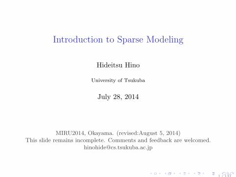
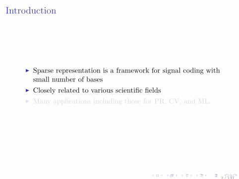
Introduction
Sparse representation is a framework for signal coding withsmall number of bases
Closely related to various scientific fields
Many applications including those for PR, CV, and ML.
2 / 131
Introduction
Sparse representation is a framework for signal coding withsmall number of bases
Closely related to various scientific fields
Many applications including those for PR, CV, and ML.
2 / 131
Introduction
Sparse representation is a framework for signal coding withsmall number of bases
Closely related to various scientific fields
Many applications including those for PR, CV, and ML.
2 / 131
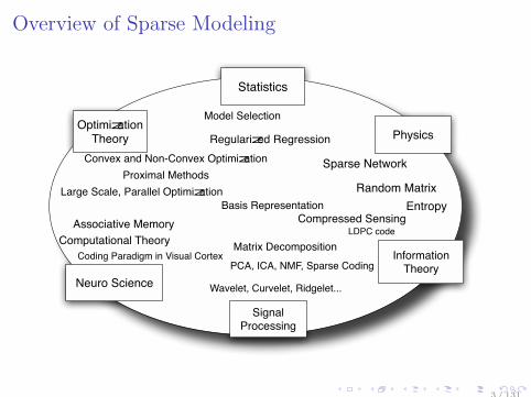
Overview of Sparse Modeling
Neuro Science
Statistics
Optimization Theory Physics
Information
Theory
Signal Processing
Model Selection
Regularized Regression
Convex and Non-Convex Optimization
Random Matrix
Compressed Sensing
Matrix DecompositionComputational Theory
Wavelet, Curvelet, Ridgelet...
PCA, ICA, NMF, Sparse Coding
Basis Representation
Coding Paradigm in Visual Cortex
Large Scale, Parallel Optimization
Sparse Network
Entropy
Associative MemoryLDPC code
Proximal Methods
3 / 131

Today’s pointSparse Modeling
Overview of Sparse Modeling
Why and how sparse modeling (sometimes) works ?
How to formulate and solve the problem ?
Applications
4 / 131

Today’s pointSparse Modeling
Overview of Sparse Modeling
Why and how sparse modeling (sometimes) works ?
How to formulate and solve the problem ?
Applications
4 / 131

Today’s pointSparse Modeling
Overview of Sparse Modeling
Why and how sparse modeling (sometimes) works ?
How to formulate and solve the problem ?
Applications
4 / 131

Today’s pointSparse Modeling
Overview of Sparse Modeling
Why and how sparse modeling (sometimes) works ?
How to formulate and solve the problem ?
Applications
4 / 131

Index
PreliminaryNotation and Problem SettingMatrix Decomposition
Mathematical Background
Computations
Applications
Perspective
5 / 131
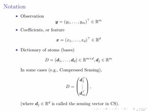
Notation
Observationy = (y1, . . . , ym)⊤ ∈ Rm
Coefficients, or feature
x = (x1, . . . , xd)⊤ ∈ Rd
Dictionary of atoms (bases)
D = (d1, . . . ,dd) ∈ Rm×d,dj ∈ Rm
In some cases (e.g., Compressed Sensing),
D =
d⊤1...
d⊤m
,
(where dj ∈ Rd is called the sensing vector in CS).
6 / 131
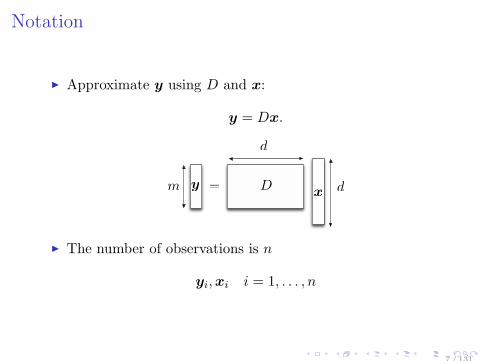
Notation
Approximate y using D and x:
y = Dx.
dDx
m y
d
=
The number of observations is n
yi,xi i = 1, . . . , n
7 / 131
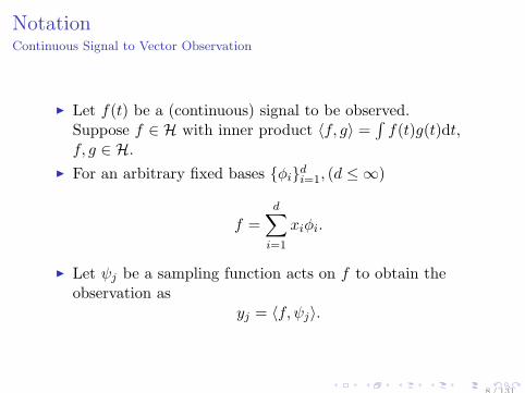
NotationContinuous Signal to Vector Observation
Let f(t) be a (continuous) signal to be observed.Suppose f ∈ H with inner product ⟨f, g⟩ =
∫f(t)g(t)dt,
f, g ∈ H.
For an arbitrary fixed bases ϕidi=1, (d ≤ ∞)
f =
d∑i=1
xiϕi.
Let ψj be a sampling function acts on f to obtain theobservation as
yj = ⟨f, ψj⟩.
8 / 131
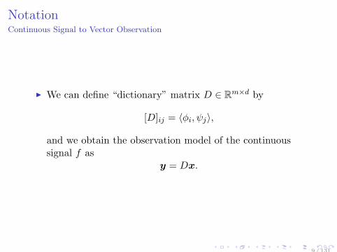
NotationContinuous Signal to Vector Observation
We can define “dictionary” matrix D ∈ Rm×d by
[D]ij = ⟨ϕi, ψj⟩,
and we obtain the observation model of the continuoussignal f as
y = Dx.
9 / 131
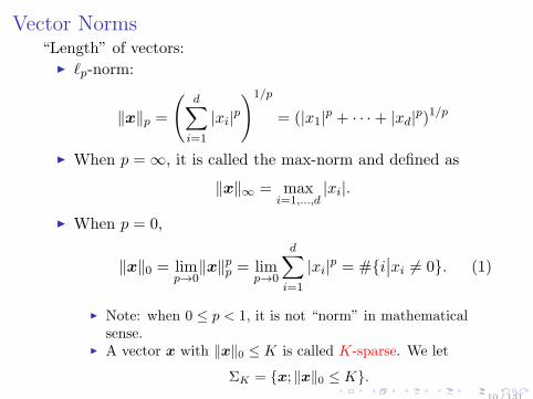
Vector Norms“Length” of vectors:
ℓp-norm:
∥x∥p =
(d∑
i=1
|xi|p)1/p
= (|x1|p + · · ·+ |xd|p)1/p
When p = ∞, it is called the max-norm and defined as
∥x∥∞ = maxi=1,...,d
|xi|.
When p = 0,
∥x∥0 = limp→0
∥x∥pp = limp→0
d∑i=1
|xi|p = #i∣∣xi = 0. (1)
Note: when 0 ≤ p < 1, it is not “norm” in mathematicalsense.
A vector x with ∥x∥0 ≤ K is called K-sparse. We let
ΣK = x; ∥x∥0 ≤ K.10 / 131
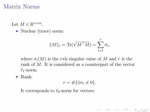
Matrix Norms
Let M ∈ Rn×m.
Nuclear (trace) norm:
∥M∥∗ = Tr(√M⊤M) =
r∑i=1
σi,
where σi(M) is the i-th singular value of M and r is therank of M . It is considered as a counterpart of the vectorℓ1-norm.
Rank:r = #i|σi = 0.
It corresponds to ℓ0-norm for vectors.
11 / 131
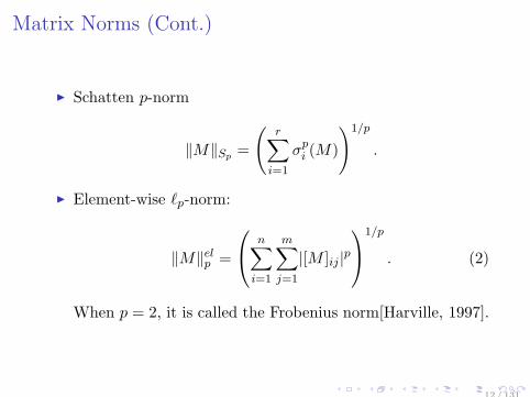
Matrix Norms (Cont.)
Schatten p-norm
∥M∥Sp =
(r∑
i=1
σpi (M)
)1/p
.
Element-wise ℓp-norm:
∥M∥elp =
n∑i=1
m∑j=1
|[M ]ij |p1/p
. (2)
When p = 2, it is called the Frobenius norm[Harville, 1997].
12 / 131
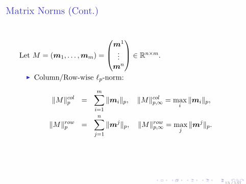
Matrix Norms (Cont.)
Let M = (m1, . . . ,mm) =
m1
...mn
∈ Rn×m.
Column/Row-wise ℓp-norm:
∥M∥colp =
m∑i=1
∥mi∥p, ∥M∥colp,∞ = maxi
∥mi∥p,
∥M∥rowp =n∑
j=1
∥mj∥p, ∥M∥rowp,∞ = maxj
∥mj∥p.
13 / 131
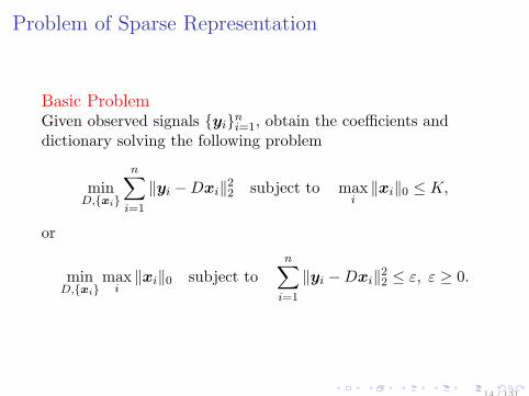
Problem of Sparse Representation
Basic ProblemGiven observed signals yini=1, obtain the coefficients anddictionary solving the following problem
minD,xi
n∑i=1
∥yi −Dxi∥22 subject to maxi
∥xi∥0 ≤ K,
or
minD,xi
maxi
∥xi∥0 subject ton∑
i=1
∥yi −Dxi∥22 ≤ ε, ε ≥ 0.
14 / 131
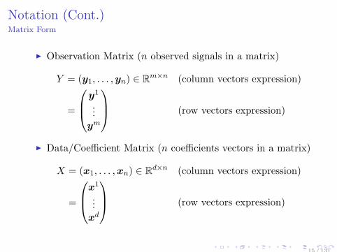
Notation (Cont.)Matrix Form
Observation Matrix (n observed signals in a matrix)
Y = (y1, . . . ,yn) ∈ Rm×n (column vectors expression)
=
y1
...ym
(row vectors expression)
Data/Coefficient Matrix (n coefficients vectors in a matrix)
X = (x1, . . . ,xn) ∈ Rd×n (column vectors expression)
=
x1
...xd
(row vectors expression)
15 / 131
Problem of Sparse Representation
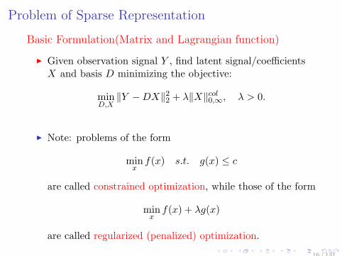
Basic Formulation(Matrix and Lagrangian function)
Given observation signal Y , find latent signal/coefficientsX and basis D minimizing the objective:
minD,X
∥Y −DX∥22 + λ∥X∥col0,∞, λ > 0.
Note: problems of the form
minxf(x) s.t. g(x) ≤ c
are called constrained optimization, while those of the form
minxf(x) + λg(x)
are called regularized (penalized) optimization.
16 / 131
Generalization
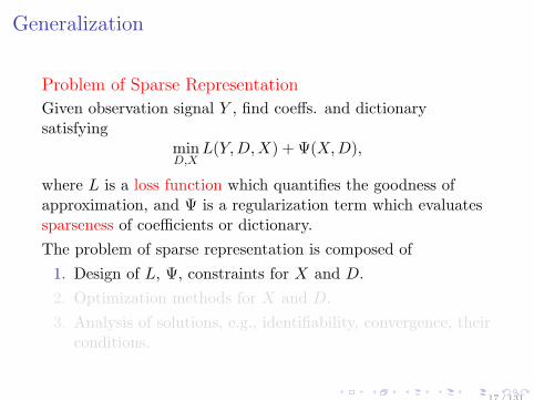
Problem of Sparse Representation
Given observation signal Y , find coeffs. and dictionarysatisfying
minD,X
L(Y,D,X) + Ψ(X,D),
where L is a loss function which quantifies the goodness ofapproximation, and Ψ is a regularization term which evaluatessparseness of coefficients or dictionary.
The problem of sparse representation is composed of
1. Design of L, Ψ, constraints for X and D.
2. Optimization methods for X and D.
3. Analysis of solutions, e.g., identifiability, convergence, theirconditions.
17 / 131
Generalization
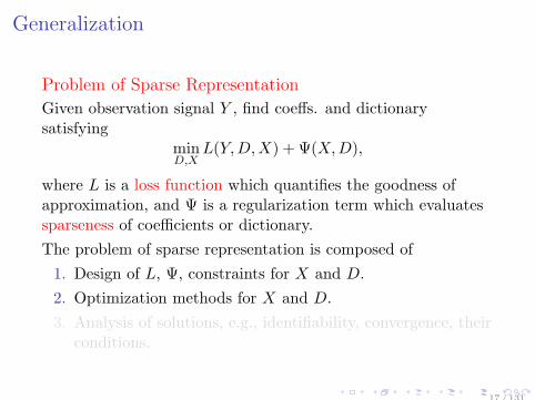
Problem of Sparse Representation
Given observation signal Y , find coeffs. and dictionarysatisfying
minD,X
L(Y,D,X) + Ψ(X,D),
where L is a loss function which quantifies the goodness ofapproximation, and Ψ is a regularization term which evaluatessparseness of coefficients or dictionary.
The problem of sparse representation is composed of
1. Design of L, Ψ, constraints for X and D.
2. Optimization methods for X and D.
3. Analysis of solutions, e.g., identifiability, convergence, theirconditions.
17 / 131
Generalization
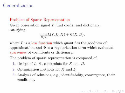
Problem of Sparse Representation
Given observation signal Y , find coeffs. and dictionarysatisfying
minD,X
L(Y,D,X) + Ψ(X,D),
where L is a loss function which quantifies the goodness ofapproximation, and Ψ is a regularization term which evaluatessparseness of coefficients or dictionary.
The problem of sparse representation is composed of
1. Design of L, Ψ, constraints for X and D.
2. Optimization methods for X and D.
3. Analysis of solutions, e.g., identifiability, convergence, theirconditions.
17 / 131
Index
PreliminaryNotation and Problem SettingMatrix Decomposition
Sparse Coding: SCPrincipal Component Analysis: PCAIndependent Component Analysis:ICANon-negative Matrix Factorization: NMF
Mathematical Background
Computations
Applications
Perspective
18 / 131
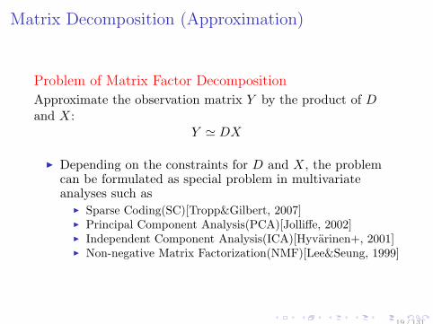
Matrix Decomposition (Approximation)
Problem of Matrix Factor Decomposition
Approximate the observation matrix Y by the product of Dand X:
Y ≃ DX
Depending on the constraints for D and X, the problemcan be formulated as special problem in multivariateanalyses such as
Sparse Coding(SC)[Tropp&Gilbert, 2007] Principal Component Analysis(PCA)[Jolliffe, 2002] Independent Component Analysis(ICA)[Hyvarinen+, 2001] Non-negative Matrix Factorization(NMF)[Lee&Seung, 1999]
19 / 131
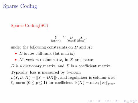
Sparse Coding
Sparse Coding(SC)
Y(m×n)
≃ D(m×d)
X(d×n)
,
under the following constraints on D and X:
D is row full-rank (fat matrix)
All vectors (columns) xi in X are sparse
D is a dictionary matrix, and X is a coefficient matrix.
Typically, loss is measured by ℓ2-normL(Y,D,X) = ∥Y −DX∥2, and regularizer is column-wiseℓp-norm (0 ≤ p ≤ 1) for coefficient Ψ(X) = maxi ∥xi∥p,∞.
20 / 131
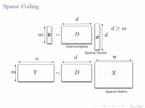
Sparse Coding
∼ dDOvercomplete x
n
m Sparse Vectory
d
∼ X
n
D
nd
m Y Sparse Matrixd ≥ m
21 / 131
Principal Component Analysis
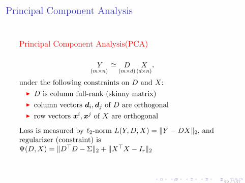
Principal Component Analysis(PCA)
Y(m×n)
≃ D(m×d)
X(d×n)
,
under the following constraints on D and X:
D is column full-rank (skinny matrix)
column vectors di,dj of D are orthogonal
row vectors xi,xj of X are orthogonal
Loss is measured by ℓ2-norm L(Y,D,X) = ∥Y −DX∥2, andregularizer (constraint) isΨ(D,X) = ∥D⊤D − Σ∥2 + ∥X⊤X − Ir∥2
22 / 131
Principal Component Analysis
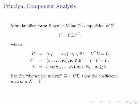
More familiar form: Singular Value Decomposition of Y
Y = UΣV ⊤,
where
U = (u1, . . . ,ur),ui ∈ Rd, U⊤U = Ir,
V ⊤ = (v1, . . . ,vn),vi ∈ Rr, V ⊤V = Ir,
Σ = diag(σ1, . . . , σr), σi ∈ R, σi ≥ 0.
Fix the “dictionary matrix” D = UΣ, then the coefficientmatrix is X = V ⊤.
23 / 131
Principal Component Analysis
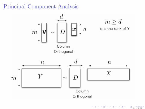
∼
dDColumn Orthogonalm
d is the rank of Ym D∼
X
dn Column Orthogonal n
xy
m ≥ dd
Y
24 / 131
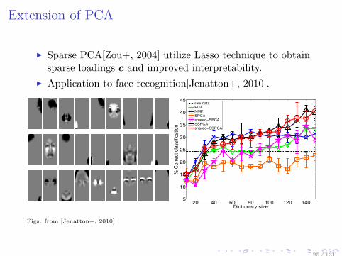
Extension of PCA
Sparse PCA[Zou+, 2004] utilize Lasso technique to obtainsparse loadings c and improved interpretability.
Application to face recognition[Jenatton+, 2010].
20 40 60 80 100 120 1405
10
15
20
25
30
35
40
45
Dictionary size
% C
orr
ect
cla
ssifi
catio
n
raw dataPCANMFSPCAshared−SPCASSPCAshared−SSPCA
Figs. from [Jenatton+, 2010]
25 / 131
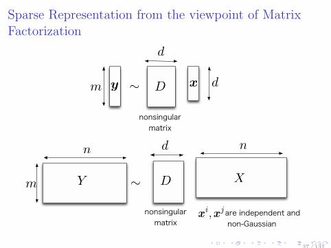
Sparse Representation from the viewpoint of MatrixFactorization
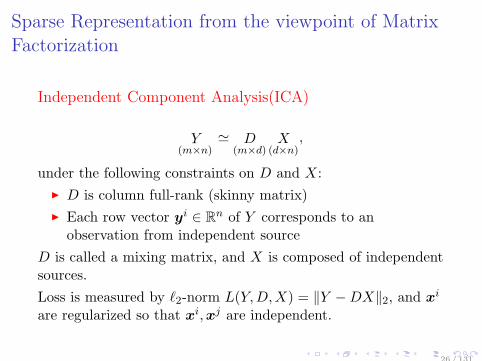
Independent Component Analysis(ICA)
Y(m×n)
≃ D(m×d)
X(d×n)
,
under the following constraints on D and X:
D is column full-rank (skinny matrix)
Each row vector yi ∈ Rn of Y corresponds to anobservation from independent source
D is called a mixing matrix, and X is composed of independentsources.
Loss is measured by ℓ2-norm L(Y,D,X) = ∥Y −DX∥2, and xi
are regularized so that xi,xj are independent.
26 / 131
Sparse Representation from the viewpoint of MatrixFactorization
∼dnonsingular matrix x
m
∼
dn are independent and non-GaussianDnonsingular matrixDm
n
y
d
XY
xi,x
j
27 / 131
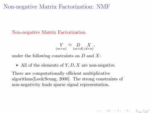
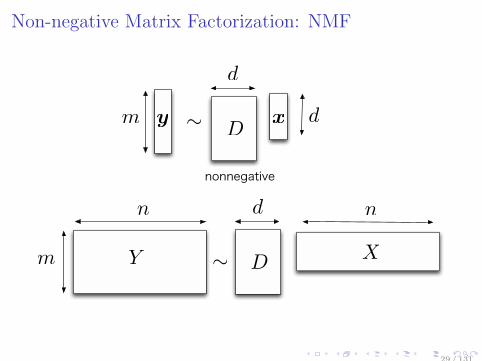
Non-negative Matrix Factorization: NMF
Non-negative Matrix Factorization
Y(m×n)
≃ D(m×d)
X(d×n)
,
under the following constraints on D and X:
All of the elements of Y,D,X are non-negative.
There are computationally efficient multiplicativealgorithms[Lee&Seung, 2000]. The strong constraints ofnon-negativity leads sparse signal representation.
28 / 131
Non-negative Matrix Factorization: NMF
∼dx
m D
nonnegative∼
X
dn
m
D
n
d
y
Y
29 / 131
Extensions of NMF
Sparse NMF[Hoyer, 2004]Non-negativity itself does not guarantee sparsity. Imposeexplicit sparsity to D or/and X.
Non-negative Tensor Factorization[Shashua&Hazan, 2005]
Sampling-based NMF[Schmidt+, 2009][Y −DX]ij ∝ N (0, σ2), [D]ij , [X]ij ∝ Exp(λ), and utilizeGibbs sampling for estimating D and X.
30 / 131
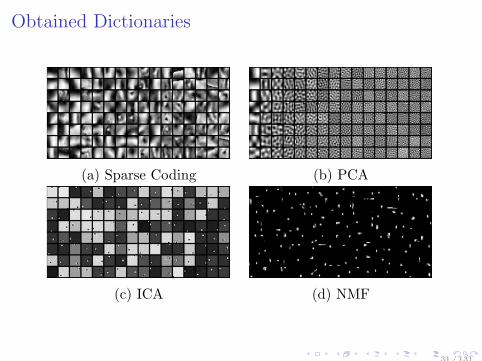
Obtained Dictionaries
(a) Sparse Coding (b) PCA
(c) ICA (d) NMF
31 / 131
Summary
Four representative matrix decomposition methods areinterpreted as different sparse models.
In next section, mathematical reasoning for the success ofsparse modeling is explained from different perspectives.
32 / 131

Index
Preliminary
Mathematical BackgroundCompressed SensingRegularized Likelihood Methods
Computations
Applications
Perspective
33 / 131
Compressed SensingOutline
A framework of recovering a sparse high-dimensional signalfrom small number of observations.
Problem setting
Exact recovery conditions Computational issue will be discussed later
34 / 131
Compressed SensingProblem Setting
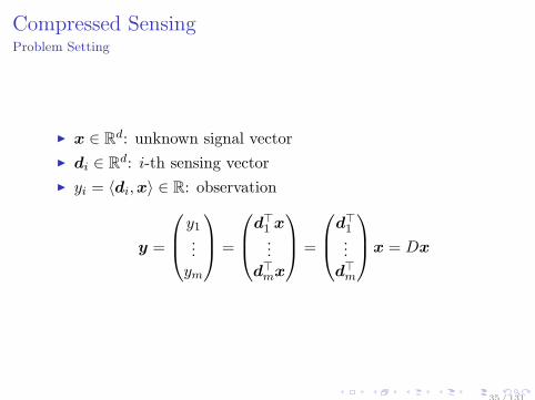
x ∈ Rd: unknown signal vector
di ∈ Rd: i-th sensing vector
yi = ⟨di,x⟩ ∈ R: observation
y =
y1...ym
=
d⊤1 x...
d⊤mx
=
d⊤1...
d⊤m
x = Dx
35 / 131
Compressed SensingProblem Setting
Usually the sensing matrix D is assumed to be known, or itcan be designed
It is also assumed that x is K-sparse, i.e.,
∥x∥0 = K.
The support of x is denoted by Ω(x), i.e., |Ω(x)| = K.
An index set is denoted as T = i1, . . . , i|T | ⊆ 1, . . . , d,and for z ∈ Rd, zT = (zi1 , . . . , ziK )
⊤ ∈ R|T | .
36 / 131
Compressed SensingProblem Setting
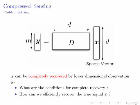
dD xm Sparse Vector=y
d
x can be completely recovered by lower dimensional observationy.
What are the conditions for complete recovery ?
How can we efficiently recover the true signal x ?
37 / 131
Compressed SensingProblem Setting
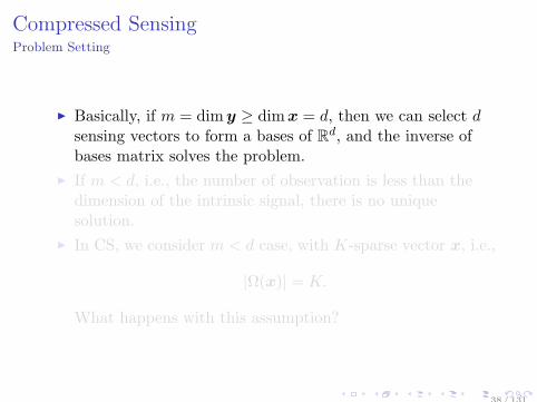
Basically, if m = dimy ≥ dimx = d, then we can select dsensing vectors to form a bases of Rd, and the inverse ofbases matrix solves the problem.
If m < d, i.e., the number of observation is less than thedimension of the intrinsic signal, there is no uniquesolution.
In CS, we consider m < d case, with K-sparse vector x, i.e.,
|Ω(x)| = K.
What happens with this assumption?
38 / 131
Compressed SensingProblem Setting
Dimension reduction and pre-image recovery.
Consider a constrained ℓp-norm minimization problem
minx
∥x∥p s.t. Dx = y, (3)
where 0 ≤ p ≤ 1.
39 / 131
Compressed SensingExact Recovery Conditions
Spark
Null Space Property (NSP)
Restricted Isometry Property (RIP)
40 / 131
Sparkexistence condition
Null space of sensing matrix D is defined by
kerD = x;Dx = 0.
Definition (Spark[Donoho&Elad, 2003])
The spark of a given matrix D is the smallest number ofcolumns of D that are linearly dependent.
TheoremFor any vector y, there exists at most one signal x ∈ ΣK suchthat y = Dx if and only if spark(D) > 2k.
proved by contradiction.
spark(D) ∈ [2,m+ 1], and the above theorem leads therequirement m ≥ 2k.
41 / 131
Null Space Property (NSP)recovery condition
Condition of the null space of sensing matrix D.
Definition (Null Space Property)
For any z ∈ kerD and for any index set T such that |T | ≤ K,the matrix D is called to have the null space property (NSP) oforder K with respect to ℓp-norm when
∥zT ∥pp < ∥zT c∥pp
holds.
42 / 131
Null Space Property (NSP)
D
RmR
d
kerD
0
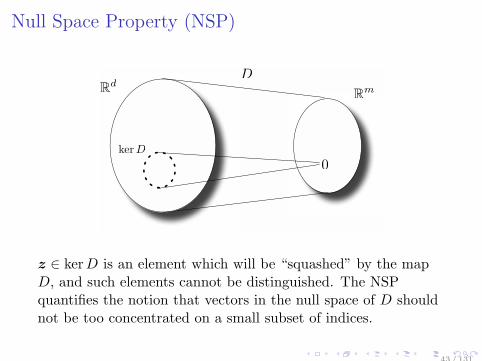
z ∈ kerD is an element which will be “squashed” by the mapD, and such elements cannot be distinguished. The NSPquantifies the notion that vectors in the null space of D shouldnot be too concentrated on a small subset of indices.
43 / 131
Null Space Property (NSP)Unique recovery theorem
Theorem (NSP for ℓp unique recovery)
For any p ∈ [0, 1], if sensing matrix D ∈ Rm×d has NSP oforder K w.r.t. ℓp-norm, then
x = arg minx∈Rd
∥x∥p s.t. y = Dx
uniquely recovers any K-sparse vector.
44 / 131
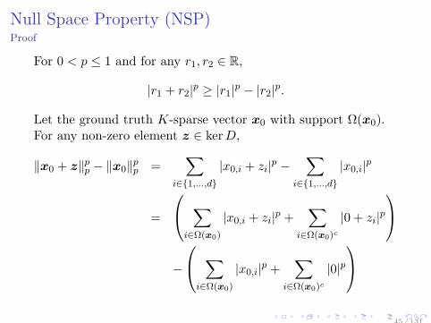
Null Space Property (NSP)Proof
For 0 < p ≤ 1 and for any r1, r2 ∈ R,
|r1 + r2|p ≥ |r1|p − |r2|p.
Let the ground truth K-sparse vector x0 with support Ω(x0).For any non-zero element z ∈ kerD,
∥x0 + z∥pp − ∥x0∥pp =∑
i∈1,...,d
|x0,i + zi|p −∑
i∈1,...,d
|x0,i|p
=
∑i∈Ω(x0)
|x0,i + zi|p +∑
i∈Ω(x0)c
|0 + zi|p
−
∑i∈Ω(x0)
|x0,i|p +∑
i∈Ω(x0)c
|0|p
45 / 131
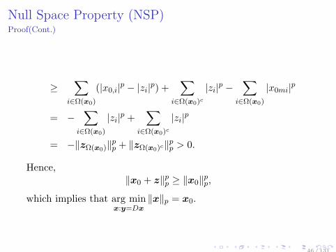
Null Space Property (NSP)Proof(Cont.)
≥∑
i∈Ω(x0)
(|x0,i|p − |zi|p) +∑
i∈Ω(x0)c
|zi|p −∑
i∈Ω(x0)
|x0mi|p
= −∑
i∈Ω(x0)
|zi|p +∑
i∈Ω(x0)c
|zi|p
= −∥zΩ(x0)∥pp + ∥zΩ(x0)c∥
pp > 0.
Hence,∥x0 + z∥pp ≥ ∥x0∥pp,
which implies that arg minx:y=Dx
∥x∥p = x0.
46 / 131
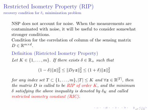
Restricted Isometry Property (RIP)recovery condition for ℓ1 minimization problem
NSP does not account for noise. When the measurements arecontaminated with noise, it will be useful to consider somewhatstronger conditions.Condition for the correlation of column of the sensing matrixD ∈ Rm×d.
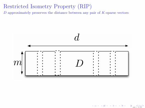
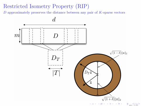
Definition (Ristricted Isometry Property)
Let K ∈ 1, . . . ,m. If there exists δ ∈ R+ such that
(1− δ)∥z∥22 ≤ ∥DTz∥22 ≤ (1 + δ)∥z∥22
for any index set T ⊂ 1, . . . ,m, |T | ≤ K and ∀z ∈ R|T |, thenthe matrix D is called to be RIP of order K, and the minimumδ satisfying the above inequality is denoted by δK and calledrestricted isometry constant (RIC).
47 / 131
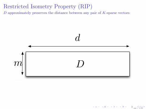
Restricted Isometry Property (RIP)D approximately preserves the distance between any pair of K-sparse vectors
D
d
m
48 / 131
Restricted Isometry Property (RIP)D approximately preserves the distance between any pair of K-sparse vectors
D
d
m
48 / 131
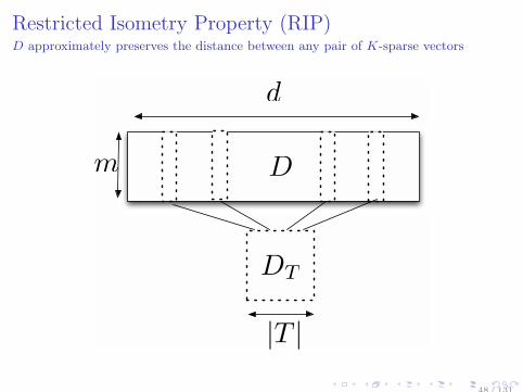
Restricted Isometry Property (RIP)D approximately preserves the distance between any pair of K-sparse vectors
D
d
m
|T |
DT
48 / 131
Restricted Isometry Property (RIP)D approximately preserves the distance between any pair of K-sparse vectors
D
d
m
|T |
DT
DTz
√
(1 + δ)‖z‖2
√
(1− δ)‖z‖2
z
48 / 131
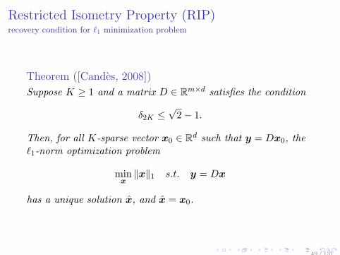
Restricted Isometry Property (RIP)recovery condition for ℓ1 minimization problem
Theorem ([Candes, 2008])
Suppose K ≥ 1 and a matrix D ∈ Rm×d satisfies the condition
δ2K ≤√2− 1.
Then, for all K-sparse vector x0 ∈ Rd such that y = Dx0, theℓ1-norm optimization problem
minx
∥x∥1 s.t. y = Dx
has a unique solution x, and x = x0.
49 / 131
Index
Preliminary
Mathematical BackgroundCompressed SensingRegularized Likelihood Methods
Computations
Applications
Perspective
50 / 131
Regularized(Penalized) Likelihood MethodsOutline
Penalized likelihood methods for regression is another approachfor understanding the sparse modeling
Methodologies
Bayesian Counterparts
this subsection is mainly due to tutorial talk “Penalized likelihood methods for
high-dimensional pattern analysis” in ACPR2013 by Dr. Jing-Hao Xue, UCL
51 / 131
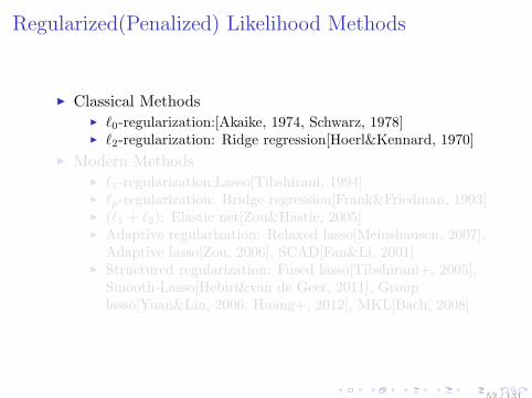
Regularized(Penalized) Likelihood Methods
Classical Methods ℓ0-regularization:[Akaike, 1974, Schwarz, 1978] ℓ2-regularization: Ridge regression[Hoerl&Kennard, 1970]
Modern Methods ℓ1-regularization:Lasso[Tibshirani, 1994] ℓp-regularization: Bridge regression[Frank&Friedman, 1993] (ℓ1 + ℓ2): Elastic net[Zou&Hastie, 2005] Adaptive regularization: Relaxed lasso[Meinshausen, 2007],
Adaptive lasso[Zou, 2006], SCAD[Fan&Li, 2001] Structured regularization: Fused lasso[Tibshirani+, 2005],
Smooth-Lasso[Hebiri&van de Geer, 2011], Grouplasso[Yuan&Lin, 2006, Huang+, 2012], MKL[Bach, 2008]
52 / 131
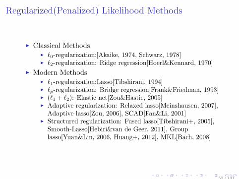
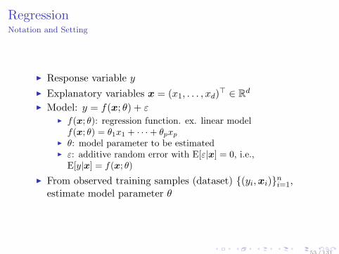
RegressionNotation and Setting
Response variable y
Explanatory variables x = (x1, . . . , xd)⊤ ∈ Rd
Model: y = f(x; θ) + ε f(x; θ): regression function. ex. linear modelf(x; θ) = θ1x1 + · · ·+ θpxp
θ: model parameter to be estimated ε: additive random error with E[ε|x] = 0, i.e.,
E[y|x] = f(x; θ)
From observed training samples (dataset) (yi,xi)ni=1,estimate model parameter θ
53 / 131
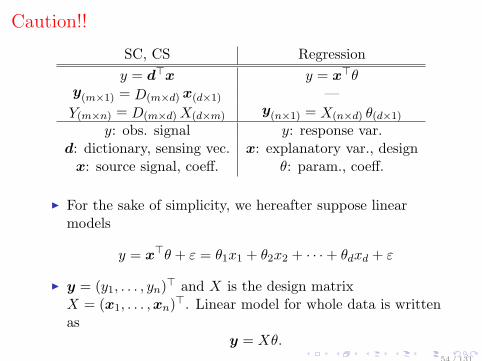
Caution!!
SC, CS Regression
y = d⊤x y = x⊤θy(m×1) = D(m×d) x(d×1) —
Y(m×n) = D(m×d)X(d×m) y(n×1) = X(n×d) θ(d×1)
y: obs. signal y: response var.d: dictionary, sensing vec. x: explanatory var., designx: source signal, coeff. θ: param., coeff.
For the sake of simplicity, we hereafter suppose linearmodels
y = x⊤θ + ε = θ1x1 + θ2x2 + · · ·+ θdxd + ε
y = (y1, . . . , yn)⊤ and X is the design matrix
X = (x1, . . . ,xn)⊤. Linear model for whole data is written
asy = Xθ.
54 / 131
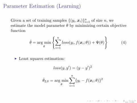
Parameter Estimation (Learning)
Given a set of training samples (yi,xi)ni=1 of size n, weestimate the model parameter θ by minimizing certain objectivefunction
θ = arg minθ
n∑
i=1
loss(yi, f(xi; θ)) + Ψ(θ)
(4)
Least squares estimation:
loss(y, y′) = (y − y′)2
θLS = arg minθ
n∑i=1
yi − f(xi; θ)2
55 / 131
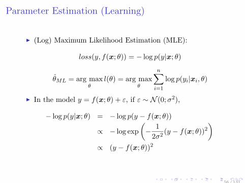
Parameter Estimation (Learning)
(Log) Maximum Likelihood Estimation (MLE):
loss(y, f(x; θ)) = − log p(y|x; θ)
θML = arg maxθ
l(θ) = arg maxθ
n∑i=1
log p(yi|xi, θ)
In the model y = f(x; θ) + ε, if ε ∼ N (0;σ2),
− log p(y|x; θ) = − log p(y − f(x; θ))
∝ − log exp
(− 1
2σ2(y − f(x; θ))2
)∝ (y − f(x; θ))2
56 / 131
Model SelectionInformation Criterion and ℓ0-regularization
Models f(x; θ):
f(x; θ) = θ1x1 + b
f(x; θ) = θ2x2 + b
f(x; θ) = θ1x1 + θ2x2 + b, etc...
One naıve way to select model is comparing ML:
θ∗ = arg maxθML
l(θML)
Problem with more features selected overfitting poor prediction for new sample less interpretable model
solution: Select fewer redundant explanatory variables, i.e.penalize larger models
57 / 131
Model SelectionInformation Criterion and ℓ0-regularization
Let K be the number of parameters in θ (recall the notion ofK-sparseness), i.e., K = ∥θ∥0.
Akaike Information Criterion (AIC:[Akaike, 1974])
AIC(θML) = −2l(θML) + 2K
Bayesian Information Criterion (BIC:[Schwarz, 1978])
BIC(θML) = −l(θML) +log n
2K
The [?]IC is
θ∗ = arg minθ
−l(θ) + λ∥θ∥0,
where λ ≥ 0 depends on the criterion.
58 / 131
Shrinking MethodsRidge: ℓ2-regularization
ℓ0 model selection θ = arg minθ
−l(θ) + λ∥θ∥0 entails a
discrete optimization
Ridge regression[Hoerl&Kennard, 1970]
θ = arg minθ
−l(θ) + λ∥θ∥22
ℓ2-regularization is strictly convex, continuous anddifferentiable
59 / 131
Shrinking MethodsRidge: ℓ2-regularization
Ridge regression shrinks θj to zero For linear models y = θ⊤x+ ε, ridge regression finds
θ = arg minθ
∥y −Xθ∥22 + λ∥θ∥22
Closed-form solution exists:
λ = 0 : θLS = (X⊤X)−1X⊤y,
λ > 0 : θ∗ = (X⊤X + λI)−1X⊤y
Assume orthonormal design X⊤X = I, then
θ∗ =1
1 + λθLS .
60 / 131
Classical regularized ML methodsℓ0 and ℓ2-regularizations
ℓ0 regularized regression:
Pros : can find parsimonious model, and introducesno bias for the estimates
Cons : entails combinatorial problem
ℓ2 regularized regression:
Pros : has closed form solution, andcomputationally efficient. It also avoidssingularity
Cons : does not select models, and introduces(sometimes severe) bias
61 / 131
Shrinking MethodsLasso: ℓ1-regularization
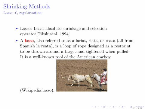
Lasso: Least absolute shrinkage and selectionoperator[Tibshirani, 1994]
A lasso, also referred to as a lariat, riata, or reata (all fromSpanish la reata), is a loop of rope designed as a restraintto be thrown around a target and tightened when pulled.It is a well-known tool of the American cowboy
(Wikipedia:lasso).
62 / 131
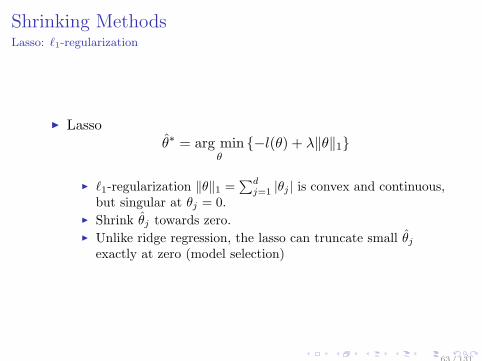
Shrinking MethodsLasso: ℓ1-regularization
Lassoθ∗ = arg min
θ−l(θ) + λ∥θ∥1
ℓ1-regularization ∥θ∥1 =∑d
j=1 |θj | is convex and continuous,but singular at θj = 0.
Shrink θj towards zero. Unlike ridge regression, the lasso can truncate small θj
exactly at zero (model selection)
63 / 131
Shrinking MethodsLasso: ℓ1-regularization
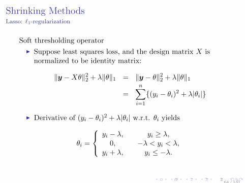
Soft thresholding operator
Suppose least squares loss, and the design matrix X isnormalized to be identity matrix:
∥y −Xθ∥22 + λ∥θ∥1 = ∥y − θ∥22 + λ∥θ∥1
=n∑
i=1
(yi − θi)2 + λ|θi|
Derivative of (yi − θi)2 + λ|θi| w.r.t. θi yields
θi =
yi − λ, yi ≥ λ,
0, −λ < yi < λ,yi + λ, yi ≤ −λ.
64 / 131
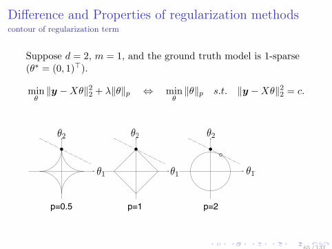
Difference and Properties of regularization methodscontour of regularization term
Suppose d = 2, m = 1, and the ground truth model is 1-sparse(θ∗ = (0, 1)⊤).
minθ
∥y −Xθ∥22 + λ∥θ∥p ⇔ minθ
∥θ∥p s.t. ∥y −Xθ∥22 = c.
x1
x2
x1
x2
x1
x2
(a) (b) (c)p=1/2 p=1 p=2
図 3: 単位 ℓp球.N = 2, |x1|p + |x2|p = 1(単位 ℓ1/2球は慨形).
x1
x2
x1
x2
x1
x2
x1
x2
(a) (b) (c) (d)
図 4: ℓp再構成.K = 1, M = 1, N = 2の場合.
1-sparse
2-sparse
x1
x2
x3
1-sparse
x1
x2
x3
1-sparse
1-sparse
2-sparse
x1
x2
x3
1-sparse
2-sparse
x1
x2
x3
(a) (b) (c) (d)
図 5: ℓp再構成.K = 1, M = 1, N = 3場合.
の情報の特徴を捉えることができる.疎な原信号は,離散信号 f ∈ RN になんらかの変換をしたとき疎になる信号として扱うことができる.すなわち,離散信号 f を既知の表現基底(例えばDCT基底,wavelet基底など)Ψ = (ψ1, · · · ,ψN) ∈ RN×N
によって,f =!N
n=1 x0,nψnのように展開して,係数の系列 x0 = (x0,1, · · · , x0,N)⊤
を原信号とする.この関係
f = Ψx0 (2)
は,表現モデルと呼ばれる.観測信号 y = (y1, · · · , yM)⊤は,既知の観測基底 Φ = (φ1, · · · ,φM) ∈ RN×M に
6
1
2
1
2
1
2
p=0.5 p=1 p=2
65 / 131
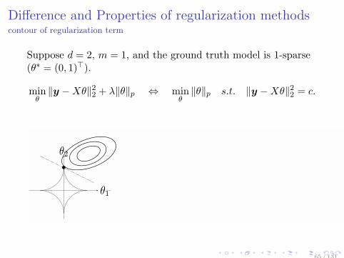
Difference and Properties of regularization methodscontour of regularization term
Suppose d = 2, m = 1, and the ground truth model is 1-sparse(θ∗ = (0, 1)⊤).
minθ
∥y −Xθ∥22 + λ∥θ∥p ⇔ minθ
∥θ∥p s.t. ∥y −Xθ∥22 = c.
x1
x2
x1
x2
x1
x2
x1
x2
(a) (b) (c) (d)
θ1
θ2
65 / 131

Difference and Properties of regularization methodscontour of regularization term
Suppose d = 2, m = 1, and the ground truth model is 1-sparse(θ∗ = (0, 1)⊤).
minθ
∥y −Xθ∥22 + λ∥θ∥p ⇔ minθ
∥θ∥p s.t. ∥y −Xθ∥22 = c.
x1
x2
x1
x2
x1
x2
(a) (b) (c)p=1/2 p=1 p=2
図 3: 単位 ℓp球.N = 2, |x1|p + |x2|p = 1(単位 ℓ1/2球は慨形).
x1
x2
x1
x2
x1
x2
x1
x2
(a) (b) (c) (d)
図 4: ℓp再構成.K = 1, M = 1, N = 2の場合.
1-sparse
2-sparse
x1
x2
x3
1-sparse
x1
x2
x3
1-sparse
1-sparse
2-sparse
x1
x2
x3
1-sparse
2-sparse
x1
x2
x3
(a) (b) (c) (d)
図 5: ℓp再構成.K = 1, M = 1, N = 3場合.
の情報の特徴を捉えることができる.疎な原信号は,離散信号 f ∈ RN になんらかの変換をしたとき疎になる信号として扱うことができる.すなわち,離散信号 f を既知の表現基底(例えばDCT基底,wavelet基底など)Ψ = (ψ1, · · · ,ψN) ∈ RN×N
によって,f =!N
n=1 x0,nψnのように展開して,係数の系列 x0 = (x0,1, · · · , x0,N)⊤
を原信号とする.この関係
f = Ψx0 (2)
は,表現モデルと呼ばれる.観測信号 y = (y1, · · · , yM)⊤は,既知の観測基底 Φ = (φ1, · · · ,φM) ∈ RN×M に
6
1
2
1
2
1
2
p=0.5 p=1 p=2
65 / 131
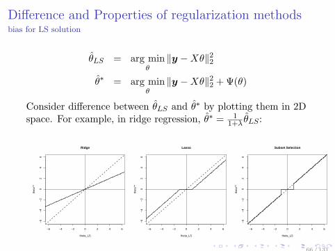
Difference and Properties of regularization methodsbias for LS solution
θLS = arg minθ
∥y −Xθ∥22
θ∗ = arg minθ
∥y −Xθ∥22 +Ψ(θ)
Consider difference between θLS and θ∗ by plotting them in 2Dspace. For example, in ridge regression, θ∗ = 1
1+λ θLS :
−6 −4 −2 0 2 4 6
−6
−4
−2
02
46
Ridge
theta_LS
thet
a^*
−6 −4 −2 0 2 4 6
−6
−4
−2
02
46
Lasso
theta_LS
thet
a^*
−6 −4 −2 0 2 4 6
−6
−4
−2
02
46
Subset Selection
theta_LSth
eta^
*
66 / 131
Generalization: More SparsityBridge Regression
Bridge regression[Frank&Friedman, 1993]
θ∗ = arg minθ
−l(θ) + λ∥θ∥pp
ℓp regularization ∥θ∥pp =∑d
j=1 |θj |p, p ≥ 0
When 0 ≤ p < 1, sparser solution than those obtained bylasso
ℓp, p < 1 regularization is non-convex
67 / 131
Generalization: Less SparsityElastic Net
When p > n, lasso only finds n non-zeros.
Lasso cannot select all of highly-correlated features.
Elastic net[Zou&Hastie, 2005]
θ∗ = arg minθ
−l(θ) + λ1∥θ∥1 + λ2∥θ∥22
ℓ1 for feature selection ℓ2 for selection of highly-correlated features
Double shrinkage introduces extra bias, which, though, canbe corrected:
Corrected elastic net: θ∗∗ = θ∗(1 + λ2). Intuitively, it cancels the shrinkage 1/(1 + λ2) caused by
ridge regression.
68 / 131
Generalization: Bias Reductionrelaxed lasso, adaptive lasso, SCAD
Relaxed lasso[Meinshausen, 2007]
Adaptive lasso[Zou, 2006]
SCAD[Fan&Li, 2001]Smoothly Clipped Absolute Deviation
69 / 131
Generalization: Bias Reductionrelaxed lasso
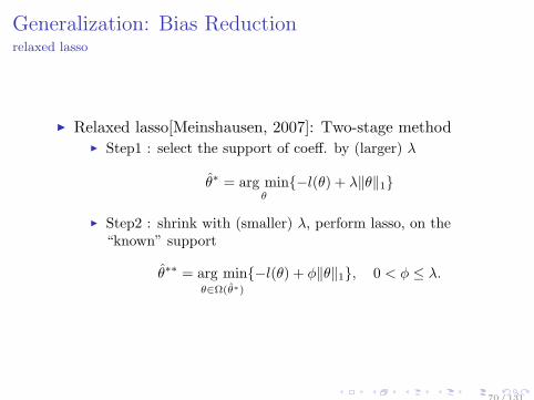
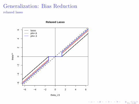
Relaxed lasso[Meinshausen, 2007]: Two-stage method Step1 : select the support of coeff. by (larger) λ
θ∗ = arg minθ
−l(θ) + λ∥θ∥1
Step2 : shrink with (smaller) λ, perform lasso, on the“known” support
θ∗∗ = arg minθ∈Ω(θ∗)
−l(θ) + ϕ∥θ∥1, 0 < ϕ ≤ λ.
70 / 131
Generalization: Bias Reductionrelaxed lasso
−6 −4 −2 0 2 4 6
−6
−4
−2
02
46
Relaxed Lasso
theta_LS
thet
a^*
lassophi=.6phi=.3
71 / 131
Generalization: Bias Reductionadaptive lasso
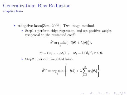
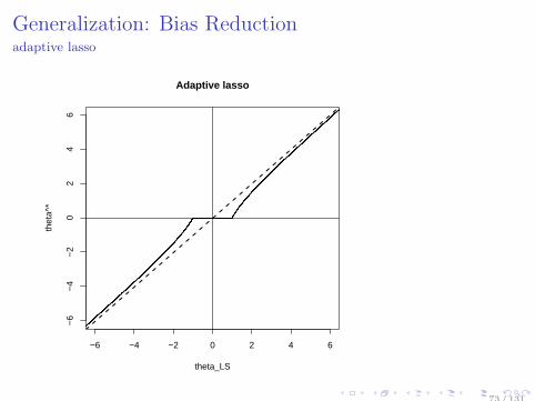
Adaptive lasso[Zou, 2006]: Two-stage method Step1 : perform ridge regression, and set positive weight
reciprocal to the estimated coeff.
θ∗ arg minθ
−l(θ) + λ∥θ∥22,
w = (w1, . . . , wd)⊤, wj = 1/|θj |ν , ν > 0.
Step2 : perform weighted lasso
θ∗∗ = arg minθ
−l(θ) + λd∑
j=1
wj |θj |
72 / 131
Generalization: Bias Reductionadaptive lasso
−6 −4 −2 0 2 4 6
−6
−4
−2
02
46
Adaptive lasso
theta_LS
thet
a^*
73 / 131
Generalization: Bias ReductionSCAD
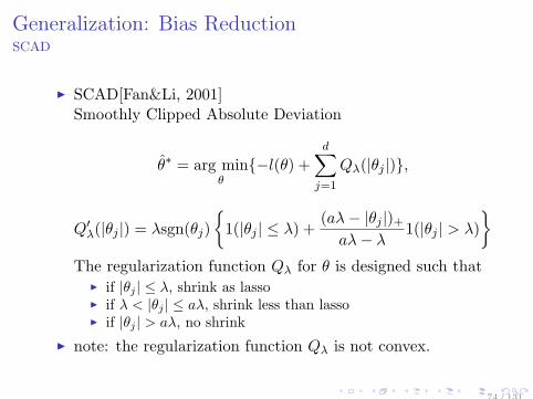
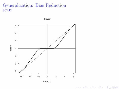
SCAD[Fan&Li, 2001]Smoothly Clipped Absolute Deviation
θ∗ = arg minθ
−l(θ) +d∑
j=1
Qλ(|θj |),
Q′λ(|θj |) = λsgn(θj)
1(|θj | ≤ λ) +
(aλ− |θj |)+aλ− λ
1(|θj | > λ)
The regularization function Qλ for θ is designed such that
if |θj | ≤ λ, shrink as lasso if λ < |θj | ≤ aλ, shrink less than lasso if |θj | > aλ, no shrink
note: the regularization function Qλ is not convex.
74 / 131
Generalization: Bias ReductionSCAD
−6 −4 −2 0 2 4 6
−6
−4
−2
02
46
SCAD
theta_LS
thet
a^*
75 / 131
Generalization: Structured SparsityFused lasso, Group lasso, MKL
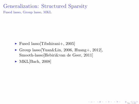
Fused lasso[Tibshirani+, 2005]
Group lasso[Yuan&Lin, 2006, Huang+, 2012],Smooth-lasso[Hebiri&van de Geer, 2011]
MKL[Bach, 2008]
76 / 131
Generalization: Structured SparsityFused lasso
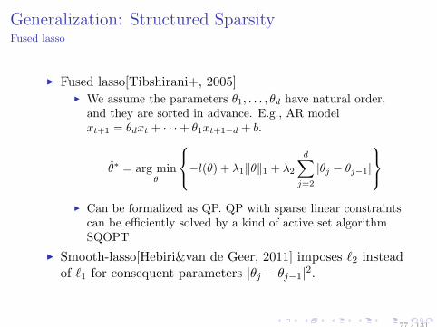
Fused lasso[Tibshirani+, 2005] We assume the parameters θ1, . . . , θd have natural order,
and they are sorted in advance. E.g., AR modelxt+1 = θdxt + · · ·+ θ1xt+1−d + b.
θ∗ = arg minθ
−l(θ) + λ1∥θ∥1 + λ2
d∑j=2
|θj − θj−1|
Can be formalized as QP. QP with sparse linear constraints
can be efficiently solved by a kind of active set algorithmSQOPT
Smooth-lasso[Hebiri&van de Geer, 2011] imposes ℓ2 insteadof ℓ1 for consequent parameters |θj − θj−1|2.
77 / 131
Generalization: Structured SparsityGroup lasso
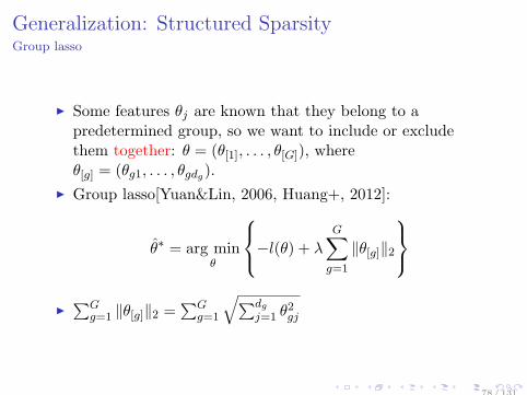
Some features θj are known that they belong to apredetermined group, so we want to include or excludethem together: θ = (θ[1], . . . , θ[G]), whereθ[g] = (θg1, . . . , θgdg).
Group lasso[Yuan&Lin, 2006, Huang+, 2012]:
θ∗ = arg minθ
−l(θ) + λ
G∑g=1
∥θ[g]∥2
∑G
g=1 ∥θ[g]∥2 =∑G
g=1
√∑dgj=1 θ
2gj
78 / 131
Generalization: Structured SparsityGroup lasso
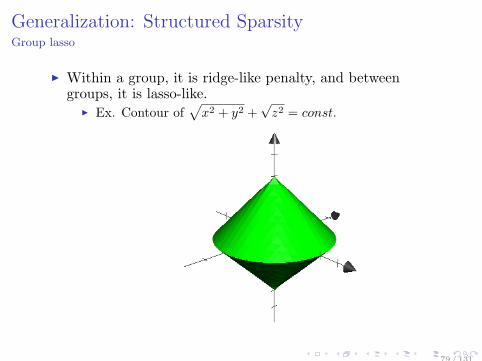
Within a group, it is ridge-like penalty, and betweengroups, it is lasso-like.
Ex. Contour of√x2 + y2 +
√z2 = const.
79 / 131
Generalization: Structured SparsityMKL
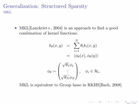
MKL[Lanckriet+, 2004] is an approach to find a goodcombination of kernel functions.
kθ(x, y) =N∑i=1
θiki(x, y)
= ⟨ϕθ(x), ϕθ(y)⟩
ϕθ =
√θ1ϕ1...√
θNϕN
, ϕi ∈ Hi.
MKL is equivalent to Group lasso in RKHS[Bach, 2008]
80 / 131
Bayesian InterpretationPreliminary
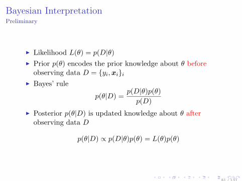
Likelihood L(θ) = p(D|θ) Prior p(θ) encodes the prior knowledge about θ before
observing data D = yi,xii Bayes’ rule
p(θ|D) =p(D|θ)p(θ)p(D)
Posterior p(θ|D) is updated knowledge about θ afterobserving data D
p(θ|D) ∝ p(D|θ)p(θ) = L(θ)p(θ)
81 / 131
Bayesian InterpretationPreliminary
θ is a random variable with pdf p(θ)
p(θ|D) ∝ L(θ)p(θ), hence log p(θ|D) = l(θ) + log p(θ) + C
Posterior mode is
θ = arg maxθ
log p(θ|D) = arg maxθ
l(θ) + log p(θ) + C
If log p(θ) = −Ψ(θ)− C, then Bayesian posterior mode isequivalent to that obtained by the regularized likelihoodmethods
θ = arg minθ
−l(θ) + Ψ(θ).
82 / 131
Bayesian InterpretationPriors for regularized methods I
Ridge regression Ψ(θ) = λ∥θ∥22 p(θ) ∝ e−Ψ(θ) = e−λ∥θ∥2
2
A Gaussian prior with mean 0, independent andhomoscedastic θj
Lasso Ψ(θ) = λ∥θ∥1 p(θ) ∝ e−Ψ(θ) = e−λ∥θ∥1
A Laplacian prior with mean 0, independent andhomoscedastic θj
Subset selection (e.g., AIC, BIC) Ψ(θ) = λ∥θ∥0 p(θ) ∝ e−Ψ(θ) = e−λ∥θ∥0
An improper prior
83 / 131
Bayesian InterpretationIntuitive Understanding
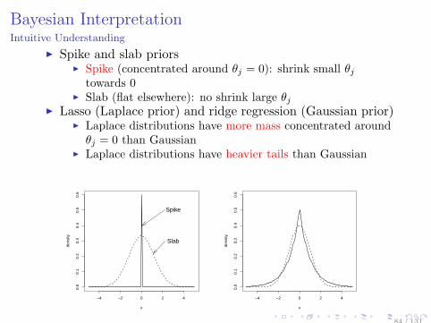
Spike and slab priors Spike (concentrated around θj = 0): shrink small θj
towards 0 Slab (flat elsewhere): no shrink large θj
Lasso (Laplace prior) and ridge regression (Gaussian prior) Laplace distributions have more mass concentrated aroundθj = 0 than Gaussian
Laplace distributions have heavier tails than Gaussian
−4 −2 0 2 4
0.0
0.1
0.2
0.3
0.4
0.5
0.6
x
dens
ity
Spike
Slab
−4 −2 0 2 4
0.0
0.1
0.2
0.3
0.4
0.5
0.6
x
dens
ity
84 / 131
Bayesian InterpretationPriors for regularized methods II
Bridge regression Ψ(θ) = λ∥θ∥pp p(θ) ∝ e−Ψ(θ) = e−λ∥θ∥p
p
An exponential-family (generalized Gaussian) prior
Elastic net Ψ(θ) = λ1∥θ∥1 + λ2∥θ∥22 p(θ) ∝ e−Ψ(θ) = e−λ1∥θ∥1−λ2∥θ∥2
2
An intermediate between the Gaussian and Laplacian priors
85 / 131
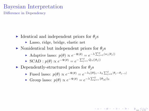
Bayesian InterpretationDifference in Dependency
Identical and independent priors for θjs Lasso, ridge, bridge, elastic net
Nonidentical but independent priors for θjs
Adaptive lasso: p(θ) ∝ e−Ψ(θ) = e−λ∑d
j=1(wj |θj |)
SCAD : p(θ) ∝ e−Ψ(θ) = e−∑d
j=1 Qλ(|θj |)
Dependently-structured priors for θjs
Fused lasso: p(θ) ∝ e−Ψ(θ) = e−λ1∥θ∥1−λ2
∑dj=2 |θj−θj−1|
Group lasso: p(θ) ∝ e−Ψ(θ) = e−λ∑G
g=1 ∥θ[g]∥2
86 / 131
Bayesian InterpretationAdvantages
Can encode prior knowledge about θ
Can obtain a posterior of θ rather than just a pointestimation of θ
Obtain the uncertainty of the selected θ Use the posterior mean E[θ|D], instead of the posterior
mode
Can sequentially update our knowledge about θ whenevernew data come: “Today’s posterior is tomorrow’s prior”
87 / 131

Index
Preliminary
Mathematical Background
ComputationsSparse CodingLearning Redundant Dictionary
Applications
Perspective
88 / 131
Sparse CodingVarious Different Formulations
Sparse coding is the problem of finding best coefficient x, whenthe dictionary D is fixed.We interchangeably use the following formulations:
∀i, minx ∥xi∥p s.t. ∥yi −Dxi∥2 ≤ ε
minx ∥Y −DX∥2 s.t. maxi ∥xi∥p ≤ K
minθ ∥y −X⊤θ∥2 + λ∥θ∥p
89 / 131
Algorithms for ℓ0-norm minimization/constrainedproblems
Orthogonal Matching Pursuit(OMP)[Rezaiifar&Krishnaprasad, 1993]
Survey Propagation[Braunstein+, 2005]
Iterative Hard Thresholding(IHT)[Blumensath&Davies, 2009]
90 / 131
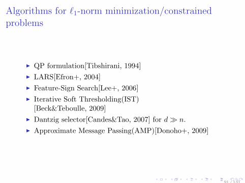
Algorithms for ℓ1-norm minimization/constrainedproblems
QP formulation[Tibshirani, 1994]
LARS[Efron+, 2004]
Feature-Sign Search[Lee+, 2006]
Iterative Soft Thresholding(IST)[Beck&Teboulle, 2009]
Dantzig selector[Candes&Tao, 2007] for d≫ n.
Approximate Message Passing(AMP)[Donoho+, 2009]
91 / 131
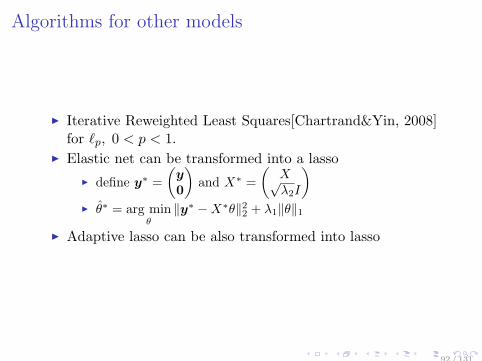
Algorithms for other models
Iterative Reweighted Least Squares[Chartrand&Yin, 2008]for ℓp, 0 < p < 1.
Elastic net can be transformed into a lasso
define y∗ =
(y0
)and X∗ =
(X√λ2I
) θ∗ = arg min
θ∥y∗ −X∗θ∥22 + λ1∥θ∥1
Adaptive lasso can be also transformed into lasso
92 / 131
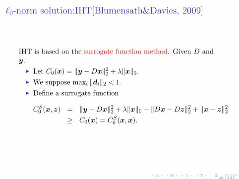
ℓ0-norm solution:IHT[Blumensath&Davies, 2009]
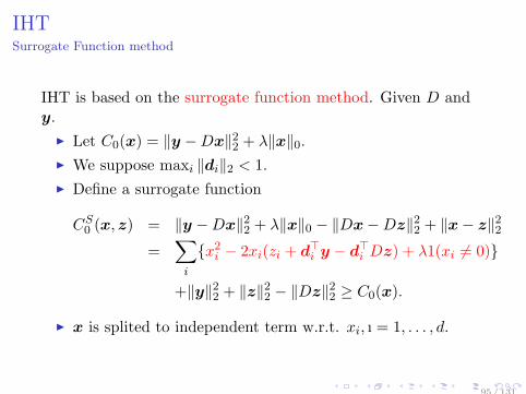
IHT is based on the surrogate function method. Given D andy.
Let C0(x) = ∥y −Dx∥22 + λ∥x∥0. We suppose maxi ∥di∥2 < 1.
Define a surrogate function
CS0 (x, z) = ∥y −Dx∥22 + λ∥x∥0 − ∥Dx−Dz∥22 + ∥x− z∥22
≥ C0(x) = CS0 (x,x).
93 / 131
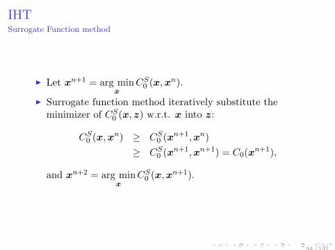
IHTSurrogate Function method
Let xn+1 = arg minx
CS0 (x,x
n).
Surrogate function method iteratively substitute theminimizer of CS
0 (x, z) w.r.t. x into z:
CS0 (x,x
n) ≥ CS0 (x
n+1,xn)
≥ CS0 (x
n+1,xn+1) = C0(xn+1),
and xn+2 = arg minx
CS0 (x,x
n+1).
94 / 131
IHTSurrogate Function method
IHT is based on the surrogate function method. Given D andy.
Let C0(x) = ∥y −Dx∥22 + λ∥x∥0. We suppose maxi ∥di∥2 < 1.
Define a surrogate function
CS0 (x, z) = ∥y −Dx∥22 + λ∥x∥0 − ∥Dx−Dz∥22 + ∥x− z∥22
=∑i
x2i − 2xi(zi + d⊤i y − d⊤
i Dz) + λ1(xi = 0)
+∥y∥22 + ∥z∥22 − ∥Dz∥22 ≥ C0(x).
x is splited to independent term w.r.t. xi, ı = 1, . . . , d.
95 / 131
IHTSurrogate Function method
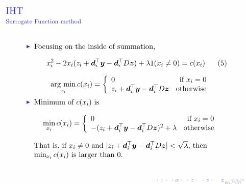
Focusing on the inside of summation,
x2i − 2xi(zi + d⊤i y − d⊤
i Dz) + λ1(xi = 0) = c(xi) (5)
arg minxi
c(xi) =
0 if xi = 0zi + d⊤
i y − d⊤i Dz otherwise
Minimum of c(xi) is
minxi
c(xi) =
0 if xi = 0−(zi + d⊤
i y − d⊤i Dz)2 + λ otherwise
That is, if xi = 0 and |zi + d⊤i y − d⊤
i Dz| <√λ, then
minxi c(xi) is larger than 0.
96 / 131
IHTSurrogate Function method
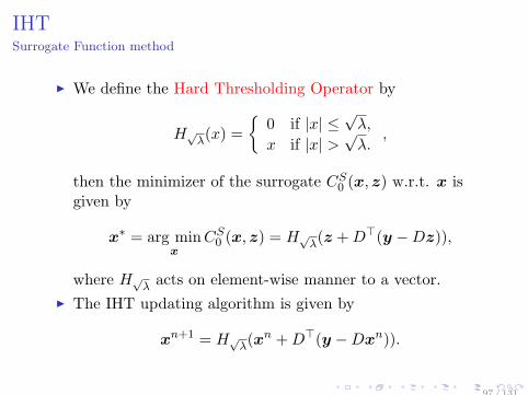
We define the Hard Thresholding Operator by
H√λ(x) =
0 if |x| ≤
√λ,
x if |x| >√λ.
,
then the minimizer of the surrogate CS0 (x,z) w.r.t. x is
given by
x∗ = arg minx
CS0 (x, z) = H√
λ(z +D⊤(y −Dz)),
where H√λ acts on element-wise manner to a vector.
The IHT updating algorithm is given by
xn+1 = H√λ(x
n +D⊤(y −Dxn)).
97 / 131
ℓ1-norm solution: QP formulation[Tibshirani, 1994]
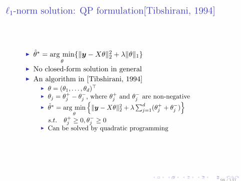
θ∗ = arg minθ
∥y −Xθ∥22 + λ∥θ∥1
No closed-form solution in general
An algorithm in [Tibshirani, 1994] θ = (θ1, . . . , θd)
⊤
θj = θ+j − θ−j , where θ+j and θ−j are non-negative
θ∗ = arg minθ
∥y −Xθ∥22 + λ
∑dj=1(θ
+j + θ−j )
s.t. θ+j ≥ 0, θ−j ≥ 0
Can be solved by quadratic programming
98 / 131
ℓp-norm solution: IRLS[Chartrand&Yin, 2008]
Iterative Reweighted Least Squares[Chartrand&Yin, 2008]:versatile method for ℓp-norm regularized problem.
Approximately solve the ℓp-norm regularized problem byiteratively solving weighted ℓ2-norm regularized problems.
99 / 131
ℓp-norm solution: IRLS[Chartrand&Yin, 2008]
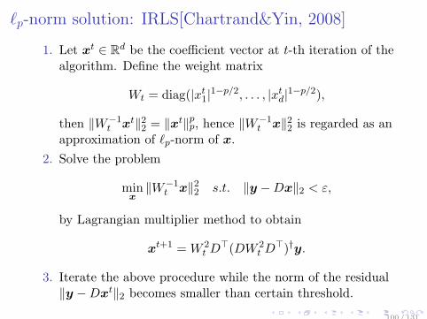
1. Let xt ∈ Rd be the coefficient vector at t-th iteration of thealgorithm. Define the weight matrix
Wt = diag(|xt1|1−p/2, . . . , |xtd|1−p/2),
then ∥W−1t xt∥22 = ∥xt∥pp, hence ∥W−1
t x∥22 is regarded as anapproximation of ℓp-norm of x.
2. Solve the problem
minx
∥W−1t x∥22 s.t. ∥y −Dx∥2 < ε,
by Lagrangian multiplier method to obtain
xt+1 =W 2t D
⊤(DW 2t D
⊤)†y.
3. Iterate the above procedure while the norm of the residual∥y −Dxt∥2 becomes smaller than certain threshold.
100 / 131

Index
Preliminary
Mathematical Background
ComputationsSparse CodingLearning Redundant Dictionary
Applications
Perspective
101 / 131
Dictionary LearningRepresentatives
Random Design Random design with Gaussian, or 0, 1binary, is known to be a good sensing matrix in CS
Fourier, Wavelet, etc. Physically interpretable, systematic bases
MOD Find a set of good bases by gradientdescent[Engan+, 1999]
K-SVD Generalization of k-means[Aharon+, 2006]
Lagrangian Dual Solve Lagrange dual to reduce the number ofvariables[Lee+, 2006]
102 / 131
K-SVD I
Most of dictionary learning methods iterate coefficient optimization with a fixed dictionary dictionary optimization with a fixed coefficient
K-SVD[Aharon+, 2006] is also a iterative method, andcoefficients are optimized by arbitrary methods for ℓ0 or ℓ1constraint problem.
Basic idea of K-SVD is, when updating the l-th basis dl,consider the error of signal approximation without usingthe basis dl, and the updated basis dl is the minimizer forthe error.
103 / 131
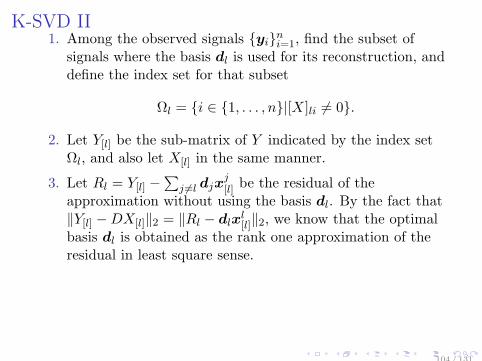
K-SVD II1. Among the observed signals yini=1, find the subset of
signals where the basis dl is used for its reconstruction, anddefine the index set for that subset
Ωl = i ∈ 1, . . . , n|[X]li = 0.
2. Let Y[l] be the sub-matrix of Y indicated by the index setΩl, and also let X[l] in the same manner.
3. Let Rl = Y[l] −∑
j =l djxj[l] be the residual of the
approximation without using the basis dl. By the fact that∥Y[l] −DX[l]∥2 = ∥Rl − dlx
l[l]∥2, we know that the optimal
basis dl is obtained as the rank one approximation of theresidual in least square sense.
104 / 131
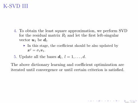
K-SVD III
4. To obtain the least square approximation, we perform SVDfor the residual matrix Rl and let the first left-singularvector u1 be dl.
In this stage, the coefficient should be also updated byxj = σ1v1.
5. Update all the bases dl, l = 1, . . . , d.
The above dictionary learning and coefficient optimization areiterated until convergence or until certain criterion is satisfied.
105 / 131
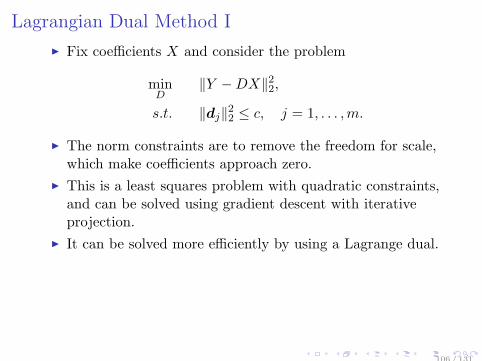
Lagrangian Dual Method I
Fix coefficients X and consider the problem
minD
∥Y −DX∥22,
s.t. ∥dj∥22 ≤ c, j = 1, . . . ,m.
The norm constraints are to remove the freedom for scale,which make coefficients approach zero.
This is a least squares problem with quadratic constraints,and can be solved using gradient descent with iterativeprojection.
It can be solved more efficiently by using a Lagrange dual.
106 / 131
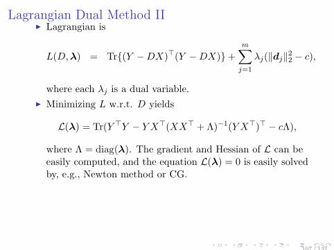
Lagrangian Dual Method II Lagrangian is
L(D,λ) = Tr(Y −DX)⊤(Y −DX)+m∑j=1
λj(∥dj∥22 − c),
where each λj is a dual variable.
Minimizing L w.r.t. D yields
L(λ) = Tr(Y ⊤Y − Y X⊤(XX⊤ + Λ)−1(Y X⊤)⊤ − cΛ),
where Λ = diag(λ). The gradient and Hessian of L can beeasily computed, and the equation L(λ) = 0 is easily solvedby, e.g., Newton method or CG.
107 / 131
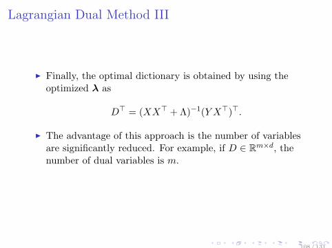
Lagrangian Dual Method III
Finally, the optimal dictionary is obtained by using theoptimized λ as
D⊤ = (XX⊤ + Λ)−1(Y X⊤)⊤.
The advantage of this approach is the number of variablesare significantly reduced. For example, if D ∈ Rm×d, thenumber of dual variables is m.
108 / 131

Index
Preliminary
Mathematical Background
Computations
Applications
Perspective
109 / 131
Applications of Sparse Modeling
Image Separation[Bobin+, 2007]
Image Restoration and Denoising[Elad&Aharon, 2006]
Face Recognition[Wright+, 2009, Zhuang+, 2014]
Image Super Resolution[Yang+, 2010, Kato+, 2014]
Recommendation System[Bell&Koren, 2007]
EEG Analysis[Cong+, 2012]
Text Classification[Berry+, 2007, Liu+, 2006]
Subspace Methods[Elhamifar&Vidal, 2013]
110 / 131
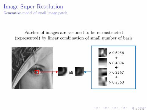
Image Super ResolutionGenerative model of small image patch
Patches of images are assumed to be reconstructed(represented) by linear combination of small number of basis
111 / 131
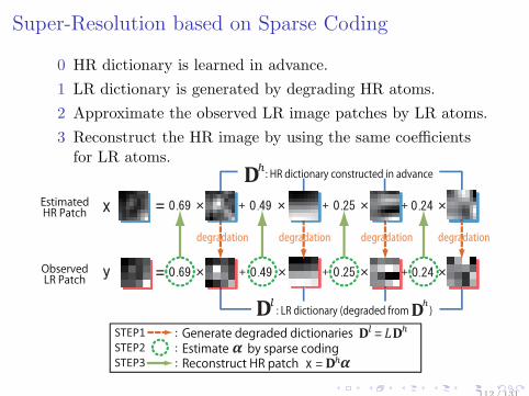
Super-Resolution based on Sparse Coding
0 HR dictionary is learned in advance.
1 LR dictionary is generated by degrading HR atoms.
2 Approximate the observed LR image patches by LR atoms.
3 Reconstruct the HR image by using the same coefficientsfor LR atoms.
112 / 131
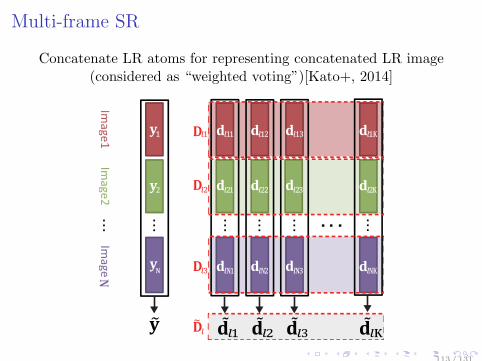
Multi-frame SR
Concatenate LR atoms for representing concatenated LR image(considered as “weighted voting”)[Kato+, 2014]
113 / 131
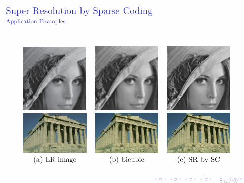
Super Resolution by Sparse CodingApplication Examples
(a) LR image (b) bicubic (c) SR by SC
114 / 131

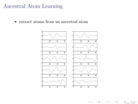
Ancestral Atom Learning
Structured Dictionary Learning: put prior information intodictionary design[Bengio+, 2009, Aharon&Elad, 2008]
Construct atoms from an “ancestral” atom Wavelet, Curvelet, Contourlet, Ridgelet
Signal decomposition by “scaled” and “shifted” atomsallows intuitive interpretation
Dictionary size to be shared is reduced
115 / 131
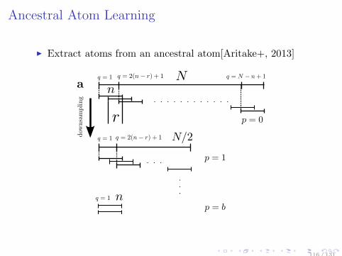
Ancestral Atom Learning
Extract atoms from an ancestral atom[Aritake+, 2013]
116 / 131
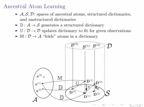
Ancestral Atom Learning A,S,D: spaces of ancestral atoms, structured dictionaries,
and unstructured dictionaries D : A → S generates a structured dictionary U : D → D updates dictionary to fit for given observations M : D → A “folds” atoms in a dictionary
117 / 131
Ancestral Atom Learning
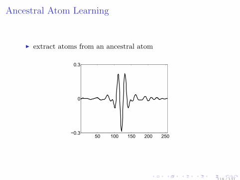
extract atoms from an ancestral atom
118 / 131
Ancestral Atom Learning
extract atoms from an ancestral atom
118 / 131

Index
Preliminary
Mathematical Background
Computations
Applications
Perspective
119 / 131
Quantum Information TheoryQuantum Tomography
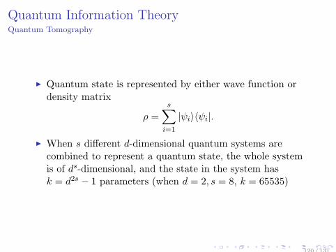
Quantum state is represented by either wave function ordensity matrix
ρ =s∑
i=1
|ψi⟩⟨ψi|.
When s different d-dimensional quantum systems arecombined to represent a quantum state, the whole systemis of ds-dimensional, and the state in the system hask = d2s − 1 parameters (when d = 2, s = 8, k = 65535)
120 / 131
Quantum Information TheoryQuantum Tomography
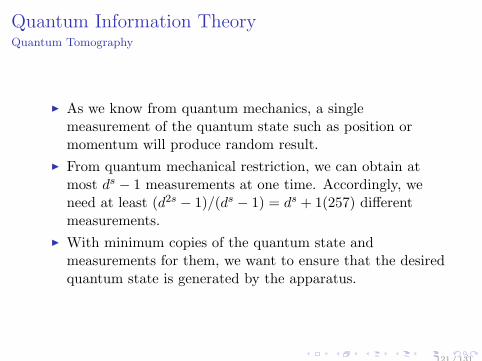
As we know from quantum mechanics, a singlemeasurement of the quantum state such as position ormomentum will produce random result.
From quantum mechanical restriction, we can obtain atmost ds − 1 measurements at one time. Accordingly, weneed at least (d2s − 1)/(ds − 1) = ds + 1(257) differentmeasurements.
With minimum copies of the quantum state andmeasurements for them, we want to ensure that the desiredquantum state is generated by the apparatus.
121 / 131

Quantum Information TheoryQuantum Tomography
T h e o p e n – a c c e s s j o u r n a l f o r p h y s i c s
New Journal of Physics
Quantum tomography via compressed sensing: error
bounds, sample complexity and efficient estimators
Steven T Flammia
1,5, David Gross
2, Yi-Kai Liu
3and Jens Eisert
4
1 Department of Computer Science and Engineering, University of Washington,Seattle, WA, USA2 Institute of Physics, University of Freiburg, 79104 Freiburg, Germany3 National Institute of Standards and Technology, Gaithersburg, MD, USA4 Dahlem Center for Complex Quantum Systems, Freie Universitat Berlin,14195 Berlin, GermanyE-mail: [email protected]
New Journal of Physics 14 (2012) 095022 (28pp)Received 23 May 2012Published 27 September 2012Online at http://www.njp.org/doi:10.1088/1367-2630/14/9/095022
Abstract. Intuitively, if a density operator has small rank, then it shouldbe easier to estimate from experimental data, since in this case only a feweigenvectors need to be learned. We prove two complementary results thatconfirm this intuition. Firstly, we show that a low-rank density matrix canbe estimated using fewer copies of the state, i.e. the sample complexity oftomography decreases with the rank. Secondly, we show that unknown low-rank states can be reconstructed from an incomplete set of measurements, usingtechniques from compressed sensing and matrix completion. These techniquesuse simple Pauli measurements, and their output can be certified without makingany assumptions about the unknown state. In this paper, we present a newtheoretical analysis of compressed tomography, based on the restricted isometryproperty for low-rank matrices. Using these tools, we obtain near-optimal errorbounds for the realistic situation where the data contain noise due to finitestatistics, and the density matrix is full-rank with decaying eigenvalues. We alsoobtain upper bounds on the sample complexity of compressed tomography, andalmost-matching lower bounds on the sample complexity of any procedure usingadaptive sequences of Pauli measurements. Using numerical simulations, we
5 Author to whom any correspondence should be addressed.
Content from this work may be used under the terms of the Creative Commons Attribution-NonCommercial-ShareAlike 3.0 licence. Any further distribution of this work must maintain attribution to the author(s) and the title
of the work, journal citation and DOI.
New Journal of Physics 14 (2012) 0950221367-2630/12/095022+28$33.00 © IOP Publishing Ltd and Deutsche Physikalische Gesellschaft
122 / 131
SummaryTake-home messages
Overviewed the sparse modeling
Related sparse modeling to various matrix decompositionmodels
Theoretically investigate why and when sparse modelingworks
Introduced some regression models, explicitly show relationto CS and SC
Explained some optimization algorithms
123 / 131
Acknowledgement
This presentation is partly based on collaboration with
Noboru Murata (Waseda Univ.)
Toshiyuki Kato (Waseda Univ.)
Toshimitsu Aritake (Hitachi, ltd.)
The presenter is supported by
JSPS Grant-in-Aid for Scientific Research on InnovativeAreas No.26120504
JSPS Grant-in-Aid for Young Scientists (B) No.25870811.
124 / 131
References I
[Aharon&Elad, 2008] Aharon, M. and Elad, M. (2008).Sparse and redundant modeling of image content using an image-signature-dictionary.SIAM J. Imaging Sciences, 1(3):228–247.
[Aharon+, 2006] Aharon, M., Elad, M., and Bruckstein, A. (2006).K-SVD: An algorithm for designing overcomplete dictionaries for sparse representation.IEEE Trans. Signal Processing, 54(11):4311–4322.
[Akaike, 1974] Akaike, H. (1974).A new look at the statistical model identification.IEEE Transactions on Automatic Control, 19(6):716–723.
[Aritake+, 2013] Aritake, T., Hino, H., and Murata, N. (2013).Learning ancestral atom via sparse coding.J. Sel. Topics Signal Processing, 7(4):586–594.
[Bach, 2008] Bach, F. R. (2008).Consistency of the group lasso and multiple kernel learning.J. Mach. Learn. Res., 9:1179–1225.
[Beck&Teboulle, 2009] Beck, A. and Teboulle, M. (2009).A fast iterative shrinkage-thresholding algorithm for linear inverse problems.SIAM J. Img. Sci., 2(1):183–202.
[Bell&Koren, 2007] Bell, R. M. and Koren, Y. (2007).Lessons from the netflix prize challenge.SIGKDD Explorations, 9(2):75–79.
[Bengio+, 2009] Bengio, S., Pereira, F., Singer, Y., and Strelow, D. (2009).Group sparse coding.In Bengio, Y., Schuurmans, D., Lafferty, J., Williams, C., and Culotta, A., editors, Advancesin Neural Information Processing Systems 22, pages 82–89. Curran Associates, Inc.
125 / 131
References II
[Berry+, 2007] Berry, M. W., Browne, M., Langville, A. N., Pauca, V. P., and Plemmons,R. J. (2007).Algorithms and applications for approximate nonnegative matrix factorization.Computational Statistics & Data Analysis, 52(1):155–173.
[Blumensath&Davies, 2009] Blumensath, T. and Davies, M. E. (2009).Iterative hard thresholding for compressed sensing.Applied and Computational Harmonic Analysis, 27(3):265 – 274.
[Bobin+, 2007] Bobin, J., luc Starck, J., Fadili, J. M., Moudden, Y., and Donoho, D. L.(2007).Morphological component analysis: An adaptive thresholding strategy.IEEE Transactions on Image Processing, 16:2675–2681.
[Braunstein+, 2005] Braunstein, A., Mezard, M., and Zecchina, R. (2005).Survey propagation: An algorithm for satisfiability.Random Struct. Algorithms, 27(2):201–226.
[Candes&Tao, 2007] Candes, E. and Tao, T. (2007).The dantzig selector: Statistical estimation when p is much larger than n.The Annals of Statistics, 35(6):pp. 2313–2351.
[Candes, 2008] Candes, E. J. (2008).The restricted isometry property and its implications for compressed sensing.Comptes Rendus Mathematique, 346(9):589–592.
[Chartrand&Yin, 2008] Chartrand, R. and Yin, W. (2008).Iteratively reweighted algorithms for compressive sensing.In ICASSP, pages 3869–3872.
126 / 131
References III
[Cong+, 2012] Cong, F., Phan, A. H., Zhao, Q., Huttunen-Scott, T., Kaartinen, J.,Ristaniemi, T., Lyytinen, H., and Cichocki, A. (2012).Benefits of multi-domain feature of mismatch negativity extracted by non-negative tensorfactorization from eeg collected by low-density array.Int. J. Neural Syst., 22(6).
[Donoho&Elad, 2003] Donoho, D. and Elad, M. (2003).
Optimally sparse representation in general (nonorthogonal) dictionaries via ℓ1
minimization.Proc. Nat. Aca. Sci., 100(5):2197–2202.
[Donoho+, 2009] Donoho, D. L., Maleki, A., and Montanari, A. (2009).Message-passing algorithms for compressed sensing.Proceedings of the National Academy of Sciences, 106(45):18914–18919.
[Efron+, 2004] Efron, B., Hastie, T., Johnstone, L., and Tibshirani, R. (2004).Least angle regression.Annals of Statistics, 32:407–499.
[Elad&Aharon, 2006] Elad, M. and Aharon, M. (2006).Image denoising via sparse and redundant representations over learned dictionaries.IEEE Trans. Image Processing, 15(12):3736–3745.
[Elhamifar&Vidal, 2013] Elhamifar, E. and Vidal, R. (2013).Sparse subspace clustering: Algorithm, theory, and applications.IEEE Trans. Pattern Anal. Mach. Intell., 35(11):2765–2781.
[Engan+, 1999] Engan, K., Aase, S. O., and Hakon Husoy, J. (1999).Method of optimal directions for frame design.In Proceedings of the Acoustics, Speech, and Signal Processing, 1999. on 1999 IEEEInternational Conference - Volume 05, ICASSP ’99, pages 2443–2446, Washington, DC, USA.IEEE Computer Society.
127 / 131
References IV
[Fan&Li, 2001] Fan, J. and Li, R. (2001).Variable selection via nonconcave penalized likelihood and its oracle properties.J. Amer. Statist. Assoc., 96(456):1348–1360.
[Frank&Friedman, 1993] Frank, I. and Friedman, J. H. (1993).A statistical view of some chemometrics regression tools.Technometrics, 35:109–148.
[Harville, 1997] Harville, D. A. (1997).Matrix Algebra from Statistician’s Perspective.Springer-Verlag, New York.
[Hebiri&van de Geer, 2011] Hebiri, M. and van de Geer, S. (2011).The smooth-lasso and other l1+l2-penalized methods.Electronic Journal of Statistics, 5:1184–1226.
[Hoerl&Kennard, 1970] Hoerl, A. E. and Kennard, R. W. (1970).Ridge regression: Biased estimation for nonorthogonal problems.Technometrics, 12:55–67.
[Hoyer, 2004] Hoyer, P. O. (2004).Non-negative matrix factorization with sparseness constraints.J. Mach. Learn. Res., 5:1457–1469.
[Huang+, 2012] Huang, J., Breheny, P., and Ma, S. (2012).A selective review of group selection in high dimensional models.Statist. Sci., 27(4):481–499.
[Hyvarinen+, 2001] Hyvarinen, A., Karhunen, J., and Oja, E. (2001).Independent Component Analysis.J. Wiley, New York.
128 / 131
References V
[Jenatton+, 2010] Jenatton, R., Obozinski, G., and Bach, F. (2010).Structured sparse principal component analysis.In AISTATS, pages 366–373.
[Jolliffe, 2002] Jolliffe, I. (2002).Principal component analysis.Springer Verlag, New York.
[Kato+, 2014] Kato, T., Hino, H., and Murata, N. (2014).Sparse coding approach for multi-frame image super resolution.CoRR, abs/1402.3926.
[Lanckriet+, 2004] Lanckriet, G. R. G., Cristianini, N., Bartlett, P., Ghaoui, L. E., andJordan, M. I. (2004).Learning the kernel matrix with semidefinite programming.J. Mach. Learn. Res., 5:27–72.
[Lee&Seung, 1999] Lee, D. D. and Seung, H. S. (1999).Learning the parts of objects by nonnegative matrix factorization.Nature, 401:788–791.
[Lee&Seung, 2000] Lee, D. D. and Seung, H. S. (2000).Algorithms for non-negative matrix factorization.In NIPS, pages 556–562.
[Lee+, 2006] Lee, H., Battle, A., Raina, R., and Ng, A. Y. (2006).Efficient sparse coding algorithms.In NIPS, pages 801–808.
[Liu+, 2006] Liu, Y., Jin, R., and Yang, L. (2006).Semi-supervised multi-label learning by constrained non-negative matrix factorization.In Proceedings of the 21st National Conference on Artificial Intelligence - Volume 1, AAAI’06,pages 421–426. AAAI Press.
129 / 131
References VI
[Meinshausen, 2007] Meinshausen, N. (2007).Relaxed lasso.Computational Statistics & Data Analysis, 52(1):374–393.
[Rezaiifar&Krishnaprasad, 1993] Rezaiifar, Y. C. P. R. and Krishnaprasad, P. S. (1993).Orthogonal matching pursuit: Recursive function approximation with applications towavelet decomposition.In Proceedings of the 27 th Annual Asilomar Conference on Signals, Systems, and Computers,pages 40–44.
[Schmidt+, 2009] Schmidt, M. N., Winther, O., and Hansen, L. (2009).Bayesian non-negative matrix factorization.Independent Component Analysis and Signal Separation, pages 540–547.
[Schwarz, 1978] Schwarz, G. (1978).Estimating the dimension of a model.The Annals of Statistics, 6:461–464.
[Shashua&Hazan, 2005] Shashua, A. and Hazan, T. (2005).Non-negative tensor factorization with applications to statistics and computer vision.In In Proceedings of the International Conference on Machine Learning (ICML, pages 792–799.ICML.
[Tibshirani, 1994] Tibshirani, R. (1994).Regression shrinkage and selection via the lasso.Journal of the Royal Statistical Society, Series B, 58:267–288.
[Tibshirani+, 2005] Tibshirani, R., Saunders, M., Rosset, S., Zhu, J., and Knight, K. (2005).Sparsity and smoothness via the fused lasso.J. R. Stat. Soc. Ser. B Stat. Methodol., 67(1):91–108.
130 / 131
References VII
[Tropp&Gilbert, 2007] Tropp, J. and Gilbert, A. (2007).Signal recovery from random measurements via orthogonal matching pursuit.Information Theory, IEEE Transactions on, 53(12):4655–4666.
[Wright+, 2009] Wright, J., Yang, A., Ganesh, A., Sastry, S., and Ma, Y. (2009).Robust face recognition via sparse representation.IEEE Transactions on Pattern Analysis and Machine Intelligence (PAMI), 31(2):210–227.
[Yang+, 2010] Yang, J., Wright, J., Huang, T. S., and Ma, Y. (2010).Image super-resolution via sparse representation.IEEE Transactions on Image Processing, 19(11):2861–2873.
[Yuan&Lin, 2006] Yuan, M. and Lin, Y. (2006).Model selection and estimation in regression with grouped variables.J. R. Stat. Soc. Ser. B Stat. Methodol., 68(1):49–67.
[Zhuang+, 2014] Zhuang, L., Chan, T.-H., Yang, A. Y., Sastry, S. S., and Ma, Y. (2014).Sparse illumination learning and transfer for single-sample face recognition with imagecorruption and misalignment.CoRR, abs/1402.1879.
[Zou, 2006] Zou, H. (2006).The adaptive lasso and its oracle properties.J. Amer. Statist. Assoc., 101(476):1418–1429.
[Zou&Hastie, 2005] Zou, H. and Hastie, T. (2005).Regularization and variable selection via the elastic net.Journal of the Royal Statistical Society, Series B, 67:301–320.
[Zou+, 2004] Zou, H., Hastie, T., and Tibshirani, R. (2004).Sparse principal component analysis.Journal of Computational and Graphical Statistics, 15:2006.
131 / 131