Embed Size (px)
Citation preview
Invariance Property and Likelihood Equation of MLEModule 4
Saurav De
Department of StatisticsPresidency University
Saurav De (Department of Statistics Presidency University)Invariance Property and Likelihood Equation of MLE 1 / 26
Invariance Property andLikelihood Equation of MLE
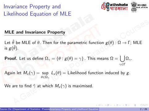
MLE and Invariance Property
Let θ be MLE of θ. Then for the parametric function g(θ) : Ω→ Γ; MLEis g(θ).
Proof. Let us define Ωγ = θ : g(θ) = γ . This means Ω =⋃γ∈Γ
Ωγ .
Again let Mx(γ) = supθ∈Ωγ
Lx(θ) = Likelihood function induced by g .
We are to find γ at which Mx(γ) is maximised.
Saurav De (Department of Statistics Presidency University)Invariance Property and Likelihood Equation of MLE 2 / 26
Invariance Property andLikelihood Equation of MLE
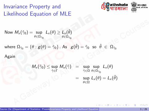
Now Mx(γ0) = supθ∈Ωγ0
Lx(θ) ≥ Lx(θ)θ∈Ωγ0
where Ωγ0 = θ : g(θ) = γ0 . As g(θ) = γ0 so θ ∈ Ωγ0
Again
Mx(γ0) ≤ supγ∈Γ
Mx(γ) = supγ∈Ω
supθ∈Ωγ0
Lx(θ)
= supθ∈Ω
Lx(θ) = Lx(θ)
Saurav De (Department of Statistics Presidency University)Invariance Property and Likelihood Equation of MLE 3 / 26
Invariance Property andLikelihood Equation of MLE
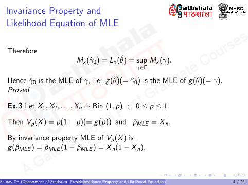
ThereforeMx(γ0) = Lx(θ) = sup
γ∈ΓMx(γ).
Hence γ0 is the MLE of γ, i.e. g(θ)(= γ0) is the MLE of g(θ)(= γ).Proved
Ex.3 Let X1,X2, . . . ,Xn ∼ Bin (1, p) ; 0 ≤ p ≤ 1
Then Vp(X ) = p(1− p)(= g(p)) and pMLE = X n.
By invariance property MLE of Vp(X ) isg(pMLE ) = pMLE (1− pMLE ) = X n(1− X n).
Saurav De (Department of Statistics Presidency University)Invariance Property and Likelihood Equation of MLE 4 / 26
Invariance Property andLikelihood Equation of MLE
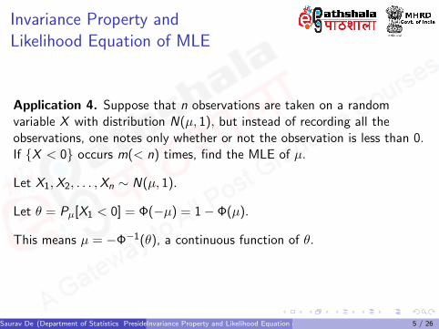
Application 4. Suppose that n observations are taken on a randomvariable X with distribution N(µ, 1), but instead of recording all theobservations, one notes only whether or not the observation is less than 0.If X < 0 occurs m(< n) times, find the MLE of µ.
Let X1,X2, . . . ,Xn ∼ N(µ, 1).
Let θ = Pµ[X1 < 0] = Φ(−µ) = 1− Φ(µ).
This means µ = −Φ−1(θ), a continuous function of θ.
Saurav De (Department of Statistics Presidency University)Invariance Property and Likelihood Equation of MLE 5 / 26
Invariance Property andLikelihood Equation of MLE
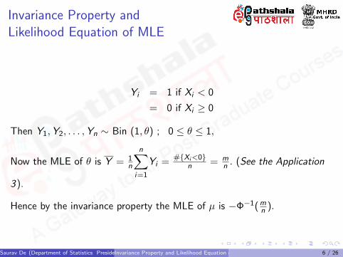
Yi = 1 if Xi < 0
= 0 if Xi ≥ 0
Then Y1,Y2, . . . ,Yn ∼ Bin (1, θ) ; 0 ≤ θ ≤ 1,
Now the MLE of θ is Y = 1n
n∑i=1
Yi = #Xi<0n = m
n . (See the Application
3).
Hence by the invariance property the MLE of µ is −Φ−1(mn ).
Saurav De (Department of Statistics Presidency University)Invariance Property and Likelihood Equation of MLE 6 / 26

Invariance Property andLikelihood Equation of MLE
Application. A commuter trip consists of first riding a subway to the busstop and then taking a bus. The bus she should like to catch arrivesuniformly over the interval θ1 to θ2. She would like to estimate both θ1 andθ2 so that she would have some idea about the time she should be at thebus stop (θ1) and she should have too late and wait for the next bus (θ2).Over an 8-day period she makes certain to be at the bus stop so early notto miss the bus and records the following arrival time of the bus.
5:15 PM , 5:21 PM , 5:14 PM , 5:23 PM , 5:29 PM , 5:17 PM, 5:15 PM , 5:18 PM
Estimate θ1 and θ2. Also give the MLEs for the mean and the variability ofthe arrival distribution.
Saurav De (Department of Statistics Presidency University)Invariance Property and Likelihood Equation of MLE 7 / 26
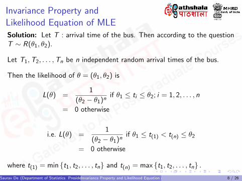
Invariance Property andLikelihood Equation of MLESolution: Let T : arrival time of the bus. Then according to the questionT ∼ R(θ1, θ2).
Let T1,T2, . . . ,Tn be n independent random arrival times of the bus.
Then the likelihood of θ = (θ1, θ2) is
L(θ) =1
(θ2 − θ1)nif θ1 ≤ ti ≤ θ2; i = 1, 2, . . . , n
= 0 otherwise
i.e. L(θ) =1
(θ2 − θ1)nif θ1 ≤ t(1) < t(n) ≤ θ2
= 0 otherwise
where t(1) = min t1, t2, . . . , tn and t(n) = max t1, t2, . . . , tn .Saurav De (Department of Statistics Presidency University)Invariance Property and Likelihood Equation of MLE 8 / 26
Invariance Property andLikelihood Equation of MLE
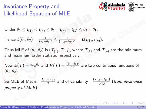
Under θ1 ≤ t(1) < t(n) ≤ θ2 , t(n) − t(1) ≤ θ2 − θ1.
Hence L(θ1, θ2) = 1(θ2−θ1)n ≤
1(t(n)−t(1))n = L(t(1), t(n)).
Thus MLE of (θ1, θ2) is (T(1),T(n)), where T(1) and T(n) are the minimumand maximum order statistic respectively.
Now E (T ) = θ1+θ22 and V (T ) = (θ2−θ1)2
12 are two continuous functions of(θ1, θ2).
So MLE of Mean :T(1)+T(n)
2 and of variability :(T(n)−T(1))√
12(from invariance
property of MLE )
Saurav De (Department of Statistics Presidency University)Invariance Property and Likelihood Equation of MLE 9 / 26

Invariance Property andLikelihood Equation of MLEComputation using R :(The minute component of the time has been considered as the data)
R Code and Output :
> samp=c(15 ,21 ,14 ,23 ,29 ,17 ,15 ,18)# given sample
> n=length(samp)# size of the sample
> n
[1] 8
> MLE_theta1=min(samp)# MLE of the parameters
> MLE_theta2=max(samp)
> MLE_theta1
[1] 14
> MLE_theta2
[1] 29
> MLE_Mean=(MLE_theta1+MLE_theta2)/2# MLE of mean
> cat("The mean arrival time is :",MLE_Mean ,"minutes after 5pm.\n")
The mean arrival time is : 21.5 minutes after 5pm.
> MLE_Var=(MLE_theta2 -MLE_theta1)/sqrt (12)# MLE of variability
> MLE_Var
[1] 4.330127
Saurav De (Department of Statistics Presidency University)Invariance Property and Likelihood Equation of MLE 10 / 26
Invariance Property andLikelihood Equation of MLE
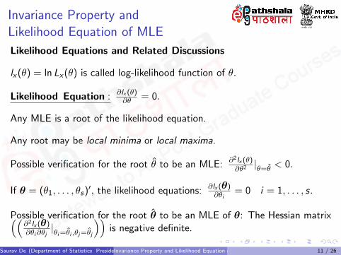
Likelihood Equations and Related Discussions
lx(θ) = ln Lx(θ) is called log-likelihood function of θ.
Likelihood Equation : ∂lx (θ)∂θ = 0.
Any MLE is a root of the likelihood equation.
Any root may be local minima or local maxima.
Possible verification for the root θ to be an MLE: ∂2lx (θ)∂θ2 |θ=θ < 0.
If θ = (θ1, . . . , θs)′, the likelihood equations: ∂lx (θ)∂θi
= 0 i = 1, . . . , s.
Possible verification for the root θ to be an MLE of θ: The Hessian matrix((∂2lx (θ)∂θi∂θj
|θi=θi ,θj=θj))
is negative definite.
Saurav De (Department of Statistics Presidency University)Invariance Property and Likelihood Equation of MLE 11 / 26
Invariance Property andLikelihood Equation of MLE
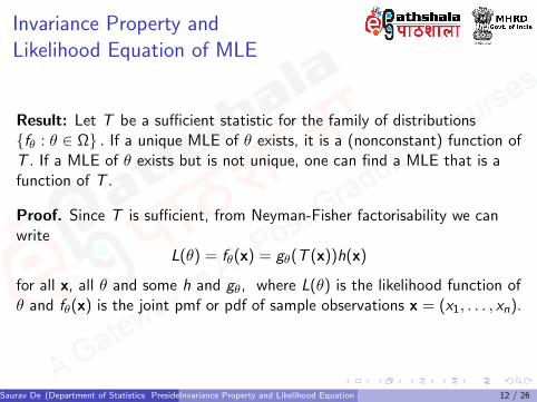
Result: Let T be a sufficient statistic for the family of distributionsfθ : θ ∈ Ω . If a unique MLE of θ exists, it is a (nonconstant) function ofT . If a MLE of θ exists but is not unique, one can find a MLE that is afunction of T .
Proof. Since T is sufficient, from Neyman-Fisher factorisability we canwrite
L(θ) = fθ(x) = gθ(T (x))h(x)
for all x, all θ and some h and gθ, where L(θ) is the likelihood function ofθ and fθ(x) is the joint pmf or pdf of sample observations x = (x1, . . . , xn).
Saurav De (Department of Statistics Presidency University)Invariance Property and Likelihood Equation of MLE 12 / 26
Invariance Property andLikelihood Equation of MLE
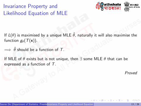
If L(θ) is maximised by a unique MLE θ, naturally it will also maximise thefunction gθ(T (x)).
=⇒ θ should be a function of T .
If MLE of θ exists but is not unique, then ∃ some MLE θ that can beexpressed as a function of T .
Proved
Saurav De (Department of Statistics Presidency University)Invariance Property and Likelihood Equation of MLE 13 / 26
Invariance Property andLikelihood Equation of MLE
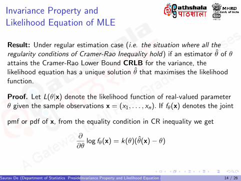
Result: Under regular estimation case (i.e. the situation where all theregularity conditions of Cramer-Rao Inequality hold) if an estimator θ of θattains the Cramer-Rao Lower Bound CRLB for the variance, thelikelihood equation has a unique solution θ that maximises the likelihoodfunction.
Proof. Let L(θ|x) denote the likelihood function of real-valued parameterθ given the sample observations x = (x1, . . . , xn). If fθ(x) denotes the joint
pmf or pdf of x, from the equality condition in CR inequality we get
∂
∂θlog fθ(x) = k(θ)(θ(x)− θ)
Saurav De (Department of Statistics Presidency University)Invariance Property and Likelihood Equation of MLE 14 / 26
Invariance Property andLikelihood Equation of MLE
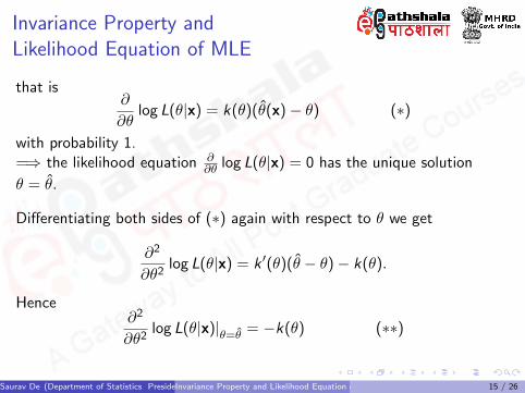
that is∂
∂θlog L(θ|x) = k(θ)(θ(x)− θ) (∗)
with probability 1.=⇒ the likelihood equation ∂
∂θ log L(θ|x) = 0 has the unique solution
θ = θ.
Differentiating both sides of (∗) again with respect to θ we get
∂2
∂θ2log L(θ|x) = k ′(θ)(θ − θ)− k(θ).
Hence∂2
∂θ2log L(θ|x)|θ=θ = −k(θ) (∗∗)
Saurav De (Department of Statistics Presidency University)Invariance Property and Likelihood Equation of MLE 15 / 26
Invariance Property andLikelihood Equation of MLE
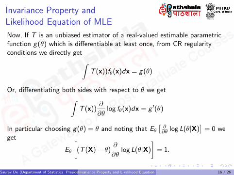
Now, If T is an unbiased estimator of a real-valued estimable parametricfunction g(θ) which is differentiable at least once, from CR regularityconditions we directly get∫
T (x))fθ(x)dx = g(θ)
Or, differentiating both sides with respect to θ we get∫T (x))
∂
∂θlog fθ(x)dx = g ′(θ)
In particular choosing g(θ) = θ and noting that Eθ[∂∂θ log L(θ|X)
]= 0 we
get
Eθ
[(T (X)− θ)
∂
∂θlog L(θ|X)
]= 1.
Saurav De (Department of Statistics Presidency University)Invariance Property and Likelihood Equation of MLE 16 / 26
Invariance Property andLikelihood Equation of MLE
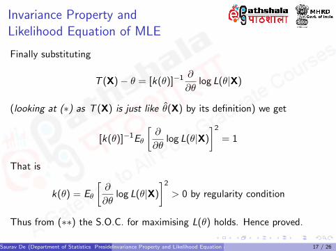
Finally substituting
T (X)− θ = [k(θ)]−1 ∂
∂θlog L(θ|X)
(looking at (∗) as T (X) is just like θ(X) by its definition) we get
[k(θ)]−1Eθ
[∂
∂θlog L(θ|X)
]2
= 1
That is
k(θ) = Eθ
[∂
∂θlog L(θ|X)
]2
> 0 by regularity condition
Thus from (∗∗) the S.O.C. for maximising L(θ) holds. Hence proved.
Saurav De (Department of Statistics Presidency University)Invariance Property and Likelihood Equation of MLE 17 / 26
Invariance Property andLikelihood Equation of MLE
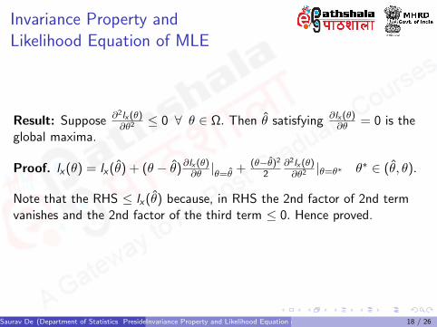
Result: Suppose ∂2lx (θ)∂θ2 ≤ 0 ∀ θ ∈ Ω. Then θ satisfying ∂lx (θ)
∂θ = 0 is theglobal maxima.
Proof. lx(θ) = lx(θ) + (θ − θ)∂lx (θ)∂θ |θ=θ + (θ−θ)2
2∂2lx (θ)∂θ2 |θ=θ∗ θ∗ ∈ (θ, θ).
Note that the RHS ≤ lx(θ) because, in RHS the 2nd factor of 2nd termvanishes and the 2nd factor of the third term ≤ 0. Hence proved.
Saurav De (Department of Statistics Presidency University)Invariance Property and Likelihood Equation of MLE 18 / 26
Invariance Property andLikelihood Equation of MLE
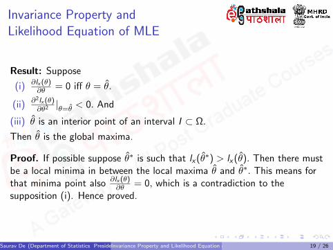
Result: Suppose
(i) ∂lx (θ)∂θ = 0 iff θ = θ.
(ii) ∂2lx (θ)∂θ2 |θ=θ < 0. And
(iii) θ is an interior point of an interval I ⊂ Ω.
Then θ is the global maxima.
Proof. If possible suppose θ∗ is such that lx(θ∗) > lx(θ). Then there mustbe a local minima in between the local maxima θ and θ∗. This means forthat minima point also ∂lx (θ)
∂θ = 0, which is a contradiction to thesupposition (i). Hence proved.
Saurav De (Department of Statistics Presidency University)Invariance Property and Likelihood Equation of MLE 19 / 26
Invariance Property andLikelihood Equation of MLE
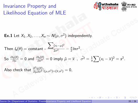
Ex.1 Let X1,X2, . . . ,Xn ∼ N(µ, σ2) independently.
Then lx(θ) = constant -
∑(xi−µ)2
2σ2 − n2 lnσ
2.
So ∂lx(θ)∂µ = 0 and ∂lx(θ)
∂σ2 = 0 imply µ = x , σ2 = 1n
∑(xi − x)2 = s2.
Also check that ∂2lx(θ)∂µ∂σ2 |(µ,σ2)=(x ,s2) = 0,
Saurav De (Department of Statistics Presidency University)Invariance Property and Likelihood Equation of MLE 20 / 26
Invariance Property andLikelihood Equation of MLE
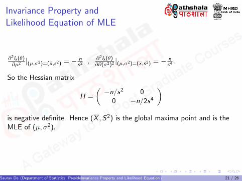
∂2lx(θ)∂µ2 |(µ,σ2)=(x ,s2) = − n
s2 , ∂2lx(θ)∂∂(σ2)2 |(µ,σ2)=(x ,s2) = − n
s4 .
So the Hessian matrix
H =
(−n/s2 0
0 −n/2s4
)is negative definite. Hence (X ,S2) is the global maxima point and is theMLE of (µ, σ2).
Saurav De (Department of Statistics Presidency University)Invariance Property and Likelihood Equation of MLE 21 / 26
Invariance Property andLikelihood Equation of MLE
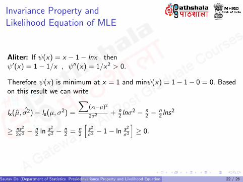
Aliter: If ψ(x) = x − 1− lnx thenψ′(x) = 1− 1/x , ψ′′(x) = 1/x2 > 0.
Therefore ψ(x) is minimum at x = 1 and minψ(x) = 1− 1− 0 = 0. Basedon this result we can write
lx(µ, σ2)− lx(µ, σ2) =
∑(xi−µ)2
2σ2 + n2 lnσ
2 − n2 −
n2 lns
2
≥ ns2
2σ2 − n2 ln s2
σ2 − n2 = n
2
[s2
σ2 − 1− ln s2
σ2
]≥ 0.
Saurav De (Department of Statistics Presidency University)Invariance Property and Likelihood Equation of MLE 22 / 26
Invariance Property andLikelihood Equation of MLE
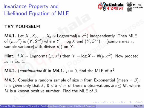
TRY YOURSELF!
M4.1. Let X1,X2, . . . ,Xn ∼ Lognormal(µ, σ2) independently. Then MLEof (µ, σ2) is (Y ,S∗2) where Y = logX and (Y ,S∗2) = (sample mean ,sample variance(with divisor n)) on Y .
Hint. If X ∼ Lognormal(µ, σ2) then Y = logX ∼ N(µ, σ2). Now proceedas in Ex. 1.
M4.2. (continuation)If in M4.1. µ = 0, find the MLE of σ2
M4.3. Consider a random sample of size n from Exponential (mean = β).It is given only that k , 0 < k < n, of these n observations are ≤ M, whereM is a known positive number. Find the MLE of β.
Saurav De (Department of Statistics Presidency University)Invariance Property and Likelihood Equation of MLE 23 / 26
Invariance Property andLikelihood Equation of MLE
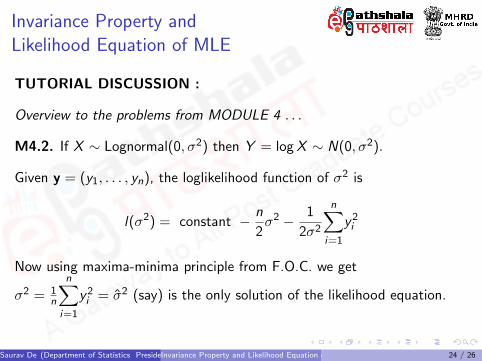
TUTORIAL DISCUSSION :
Overview to the problems from MODULE 4 . . .
M4.2. If X ∼ Lognormal(0, σ2) then Y = logX ∼ N(0, σ2).
Given y = (y1, . . . , yn), the loglikelihood function of σ2 is
l(σ2) = constant − n
2σ2 − 1
2σ2
n∑i=1
y2i
Now using maxima-minima principle from F.O.C. we get
σ2 = 1n
n∑i=1
y2i = σ2 (say) is the only solution of the likelihood equation.
Saurav De (Department of Statistics Presidency University)Invariance Property and Likelihood Equation of MLE 24 / 26
Invariance Property andLikelihood Equation of MLE
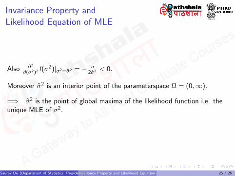
Also ∂2
∂(σ2)2 l(σ2)|σ2=σ2 = − n
2σ2 < 0.
Moreover σ2 is an interior point of the parameterspace Ω = (0,∞).
=⇒ σ2 is the point of global maxima of the likelihood function i.e. theunique MLE of σ2.
Saurav De (Department of Statistics Presidency University)Invariance Property and Likelihood Equation of MLE 25 / 26
Invariance Property andLikelihood Equation of MLE
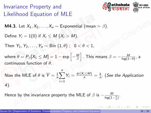
M4.3. Let X1,X2, . . . ,Xn ∼ Exponential (mean = β).
Define Yi = 1(0) if Xi ≤ M (Xi > M).
Then Y1,Y2, . . . ,Yn ∼ Bin (1, θ) ; 0 < θ < 1,
where θ = Pβ[X1 ≤ M] = 1− exp[−M
β
]. This means β = − M
log(1−θ) , a
continuous function of θ.
Now the MLE of θ is Y = 1n
n∑i=1
Yi = #Xi≤Mn = k
n . (See the Application
4).
Hence by the invariance property the MLE of β is − Mlog(1− k
n).
Saurav De (Department of Statistics Presidency University)Invariance Property and Likelihood Equation of MLE 26 / 26