Embed Size (px)
Citation preview
J.M. Burgerscentrum
Research School for Fluid Mechanics
Finite element methods for
the incompressible Navier-Stokes equations
Ir. A. Segal
2017
Delft University of TechnologyFaculty of Electrical Engineering, Mathematics and Computer ScienceDelft Institute of Applied Mathematics
Copyright 2017 by Delft Institute of Applied Mathematics, Delft, The Netherlands.
No part of this work may be reproduced, stored in a retrieval system, or transmitted, in anyform or by any means, electronic, mechanical, photocopying, recording, or otherwise, withoutthe prior written permission from Delft Institute of Applied Mathematics, Delft Universityof Technology, The Netherlands.
Contents
1 Introduction 5
2 Introduction to the finite element method 8
2.1 Differential equations and boundary conditions . . . . . . . . . . . . . . . . . 82.2 Weak formulation . . . . . . . . . . . . . . . . . . . . . . . . . . . . . . . . . . 92.3 The Galerkin method . . . . . . . . . . . . . . . . . . . . . . . . . . . . . . . 112.4 The finite element method . . . . . . . . . . . . . . . . . . . . . . . . . . . . . 122.5 Computation of the element matrix and element vector . . . . . . . . . . . . 152.6 Higher order elements . . . . . . . . . . . . . . . . . . . . . . . . . . . . . . . 172.7 Structure of the large matrix . . . . . . . . . . . . . . . . . . . . . . . . . . . 18
3 Convection-diffusion equation by the finite element method 22
3.1 Formulation of the equations . . . . . . . . . . . . . . . . . . . . . . . . . . . 223.2 Standard Galerkin . . . . . . . . . . . . . . . . . . . . . . . . . . . . . . . . . 223.3 Solution of the system of ordinary differential equations . . . . . . . . . . . . 243.4 Accuracy aspects of the SGA . . . . . . . . . . . . . . . . . . . . . . . . . . . 273.5 Streamline Upwind Petrov Galerkin . . . . . . . . . . . . . . . . . . . . . . . 303.6 Some classical benchmark problems for convection-diffusion solvers . . . . . . 35
4 Discretization of the incompressible Navier-Stokes equations by standard
Galerkin 39
4.1 The basic equations of fluid dynamics . . . . . . . . . . . . . . . . . . . . . . 394.2 Initial and boundary conditions . . . . . . . . . . . . . . . . . . . . . . . . . . 404.3 Axisymmetric flow . . . . . . . . . . . . . . . . . . . . . . . . . . . . . . . . . 424.4 The weak formulation . . . . . . . . . . . . . . . . . . . . . . . . . . . . . . . 434.5 The standard Galerkin method . . . . . . . . . . . . . . . . . . . . . . . . . . 454.6 Treatment of the non-linear terms . . . . . . . . . . . . . . . . . . . . . . . . 474.7 Necessary conditions for the elements . . . . . . . . . . . . . . . . . . . . . . . 484.8 Examples of admissible elements . . . . . . . . . . . . . . . . . . . . . . . . . 504.9 Solution of the system of linear equations due to the discretization of Navier-
Stokes . . . . . . . . . . . . . . . . . . . . . . . . . . . . . . . . . . . . . . . . 53
5 The penalty function method 56
5.1 Introduction . . . . . . . . . . . . . . . . . . . . . . . . . . . . . . . . . . . . . 565.2 The discrete penalty functions approach . . . . . . . . . . . . . . . . . . . . . 575.3 The continuous penalty function method . . . . . . . . . . . . . . . . . . . . . 585.4 Practical aspects of the penalty function method . . . . . . . . . . . . . . . . 60
6 Divergence-free elements 62
6.1 Introduction . . . . . . . . . . . . . . . . . . . . . . . . . . . . . . . . . . . . . 626.2 The construction of divergence-free basis functions for 2D elements . . . . . . 636.3 The construction of element matrices and vectors for (approximate) divergence-
free basis functions . . . . . . . . . . . . . . . . . . . . . . . . . . . . . . . . . 676.4 Boundary conditions with respect to the divergence-free elements . . . . . . . 696.5 Computation of the pressure . . . . . . . . . . . . . . . . . . . . . . . . . . . 706.6 Practical aspects of the divergence-free elements . . . . . . . . . . . . . . . . 71
3
7 The instationary Navier-Stokes equations 72
7.1 Introduction . . . . . . . . . . . . . . . . . . . . . . . . . . . . . . . . . . . . . 727.2 Solution of the instationary Navier-Stokes equations by the method of lines . 727.3 The pressure-correction method . . . . . . . . . . . . . . . . . . . . . . . . . . 74
A Derivation of the integration by parts for the momentum equations 78
4
1 Introduction
In this second course on numerical flow problems we shall focus our attention to two specificsubjects:
- the solution of the incompressible Navier-Stokes equations by finite elements;
- the efficient solution of large systems of linear equations.
Although, at first sight there seems no connection between both subjects, it must be remarkedthat the numerical solution of partial differential equations and hence also of the Navier-Stokesequations, always results in the solving of a number of large systems of sparse linear systems.Since, in general the solution of these systems and the storage of the corresponding matricestake the main part of the resources (CPU time and memory), it is very natural to studyefficient solution methods.
In the first part of these lectures we shall be concerned with the discretization of the incom-pressible Navier-Stokes equations by the finite element method (FEM). First we shall give ashort introduction of the FEM itself. The application of the FEM to potential problems isconsidered and the extension to convection-diffusion type problems is studied. The Galerkinmethod is introduced as a natural extension of the so-called weak formulation of the partialdifferential equations. One of the reasons why finite elements have been less popular in thepast than finite differences, is the lack of upwind techniques. In the last decade, however,accurate upwind methods have been constructed. The most popular one, the so-called stream-line upwind Petrov-Galerkin method (SUPG), will be treated in Chapter 3. It is shown thatupwinding may increase the quality of the solution considerably. Another important aspect ofupwinding is that it makes the systems of equations more appropriate for the iterative meth-ods treated in part II. As a consequence both the number of iterations and the computationtime decrease.In Chapter 4 the discretization of the incompressible Navier-Stokes equations is considered.Since the pressure is an unknown in the momentum equations but not in the continuity equa-tion, the discretization must satisfy some special requirements. In fact one is no longer free tochoose any combination of pressure and velocity approximation but the finite elements mustbe constructed such that the so-called Brezzi-Babuska (or BB) condition is satisfied. Thiscondition makes a relation between pressure and velocity approximation. In finite differencesand finite volumes the equivalent of the BB condition is satisfied if staggered grids are ap-plied. Even if the BB condition is satisfied we are still faced with a problem with respect tothe solution of the linear systems of equations. The absence of the pressure in the continuityequation induces zeros at some of the diagonal elements of the matrix. In general linearsolvers may be influenced by such zeros, some iterative solvers even do not allow non-positivediagonal elements. For that reason alternative solution methods have been developed, whichall try to segregate the pressure and velocity computation.Chapter 5 treats the most popular segregated method, the so-called penalty function formu-lation. In this approach the continuity equation is perturbed with a small compressibilityincluding the pressure.From this perturbed equation the pressure is expressed in terms of velocity and this is sub-stituted into the momentum equations. In this way the velocity can be computed first andafterwards the pressure. A disadvantage of this method is that the perturbation parameter
5
introduces extra complications.In Chapter 6 an alternative formulation is derived, the so-called solenoidal approach. In thismethod, the elements are constructed in such a way that the approximate divergence freedomis satisfied explicitly. To that end it is necessary to introduce the stream function as helpunknown. This method seems very attractive, however, the extension to three-dimensionalproblems is very difficult.Finally, in Chapter 7, methods for the time-dependent incompressible Navier-Stokes equa-tions are treated. For this type of methods an alternative segregation is possible, the so-calledpressure-correction method. This method is also popular in finite differences and finite vol-umes.
In the second part we consider the efficient solution of large system of linear equations. Asapplications and examples we mostly use systems of equations resulting from the discretiza-tion of 2- and 3 dimensional partial differential equations.
We start in Chapter 2.1 by considering direct methods as there are: Gaussian eliminationand Cholesky decomposition. These methods are used if the dimension of the system is nottoo large. Since these methods are implemented on computers we consider the behavior ofthe methods with respect to rounding errors. For large problems the memory requirementsof direct methods are a bottle neck, using special methods for banded, profile or ”generalsparse” matrices we can solve much larger systems. These methods only use the non zeropart of the resulting decomposition.
In Chapter 2 we consider classical iterative methods for linear equations. These methods arevery cheap with respect to memory requirements. However, convergence can be very slow sothe computing time may be much larger than for direct methods.
In Chapter 3 and 4 we consider modern iterative methods of Krylov subspace type. In Chapter3 the conjugate gradient method for symmetric positive definitive matrices, and in Chapter 4Krylov methods for general matrices. The rate of convergence is much better than for basiciterative methods, whereas no knowledge of the spectrum is needed in contrast with somebasic iterative methods. A drawback for general matrices is that there are many methodsproposed and until now there is no clear winner. We shall summarize the most successfulones and try to give some guidelines for choosing a method depending on the properties ofthe problem.
The Krylov subspace methods become much faster if they are combined with a preconditioner.For the details we refer to Chapter 5. We only note that in essence a preconditioned Krylovmethod is a combination of a method given in chapter 3 and 4 and a basic iterative methodor an incomplete direct method.
In many applications eigenvalues give information of physical properties (like eigenmodes) orthey are used to analyze, and enhance mathematical methods for solving a physical problem.If only a small number of eigenvalues are needed for a very large matrix it is a good idea touse iterative methods, which are given in Chapter 6. We start with the Power method whichis easy to understand, and approximate the largest eigenvalue. Thereafter we consider theLanczos method for symmetric matrices, which is closely related to the CG method. Againfor general matrices different methods are proposed and it is not always clear, which one is
6
the best.
Finally in Chapter 7 we give a summary of present day supercomputers. There are mainlytwo types: vector- and parallel computers. For the problems considered in this report super-computers are necessary to obtain results for large 3 dimensional problems. At this momentvector computers give the best results, with respect to computing time and memory. However,we expect that in the near future parallel computers (especially those based on a clusteringof very fast nodes) will beat them for real live problems.
7
2 Introduction to the finite element method
2.1 Differential equations and boundary conditions
The finite element method (FEM) may be considered as a general discretization tool forpartial differential equations. In this sense the FEM forms an alternative for finite differencemethods (FDM) or finite volume methods (FVM). The main reason to use the FEM is itsability to tackle relatively easily, problems that are defined on complex geometries. However,the programming of finite element methods is more complicated than that of finite differences,and hence in general requires standard software packages.
In this lecture we shall restrict ourselves to the application of the FEM to two general types ofdifferential equations: the convection-diffusion equation and the incompressible Navier-Stokesequations. The last type of equations are the subject of Chapter 4, and convection-diffusiontype of equations will be the subject of Chapter 3. In this introductory chapter we shallneglect the convective terms and focus ourselves to diffusion type problems:
ρ∂c
∂t−
n∑
i,j=1
∂
∂xi
(
aij∂c
∂xj
)
+ βc = f (1)
where c denotes the unknown, for example the potential, temperature or concentration. Thematrix A with elements aij represents the diffusion tensor and is supposed to be symmetricand positive definite. The coefficient β is zero in many practical problems, but is added forthe sake of generality. f represents a source term and ρ∂c
∂tthe time-derivative part, where
ρ must be positive in the instationary case. All coefficients ρ, aij , β and f may depend ontime and the space variable x. n is the dimension of space which in our applications variesfrom 1 to 3.If the coefficients also depend on the solution, the equations become non-linear. In thischapter we restrict ourselves to linear problems only.Equation 1 is usually written in vector notation:
ρ∂c
∂t− div (A∇c) + βc = f, (2)
where ∇ denotes the gradient operator.In this chapter we shall only consider stationary problems, so equation (2) reduces to
−div (A∇c) + βc = f (3)
In order that equation (3) has a unique solution, and to make the problem well posed it isnecessary to prescribe exactly one boundary condition at each part of the boundary. In thesequel the region at which the differential equation is defined is called Ω and its boundary isdenoted by Γ. Common boundary conditions in equation (3) are:
c = g1 on Γ1, (4)
A∇c · n = g2 on Γ2, (5)
σc+A∇c · n = g3 on Γ3 (σ ≥ 0), (6)
8
where the boundary Γ is subdivided into three parts Γ1, Γ2 and Γ3.
Boundary conditions of type (4) are called Dirichlet boundary conditions, boundary conditionsof type (5) Neumann conditions and boundary conditions of type (6) are called Robbinsboundary conditions. In fact (5) may be considered as a special case of (6).Other types of boundary conditions may also be applied, but they will not be studied in thislecture.
It can be shown that equation (3) with boundary conditions (4) to (6) has a unique solutionprovided the coefficients and the boundary of the region are sufficiently smooth. Only in thespecial case Γ1 = φ, Γ3 = φ and β = 0, the function ϕ is determined up to an additiveconstant. In that case the functions f and g2 must satisfy the compatibility condition
∫
Ω
f dΩ = −∫
Γ
g2 dΓ . (7)
(7) can be derived by integrating equation (3) over the domain Ω and applying the Gaussdivergence theorem.
2.2 Weak formulation
Before applying the FEM to solve equation (3) under the boundary conditions (4) to (6), itis necessary to transform the equation into a more suitable form. To do that there are twoalternatives:
1. one can derive an equivalent minimization problem, which has exactly the same solutionas the differential equation.
2. one can derive a so-called weak formulation.
Both methods lead finally to exactly the same result, however, since for the general equationsto be treated in Chapters 2 and 4, no equivalent minimization problem exists, we shall restrictourselves to method 2.
Originally the weak formulation has been introduced by pure mathematicians to investigatethe behavior of the solution of partial differential equations, and to prove existence anduniqueness of the solution. Later on numerical schemes have been based on this formulationwhich lead to an approximate solution in a constructive way.The weak formulation of equation (3) can be derived by multiplying (3) by a so-called testfunction v and integrating over the domain. So:
∫
Ω
(−div(A∇c) + βc) v dΩ =
∫
Ω
fv dΩ . (8)
The choice of the class of functions to which v belongs, determines whether (8) has a solutionand whether this solution is unique.It is common practice to apply integration by parts to equation (8) in order to get rid ofthe second derivative term. integration by parts is derived by applying the Gauss divergencetheorem:
∫
Ω
div a dΩ =
∫
Γ
a · n dΓ (9)
9
to the functiona = v A∇c . (10)
Hencediv a = div(vA∇c) = ∇v · A∇c+ vdiv A∇c . (11)
Substitution of (11) in (9) yields
∫
Ω
vdiv A∇c dΩ = −∫
Ω
∇v · A ∇c dΩ+
∫
Γ
v A∇c · ndΓ (12)
and so (8) can be written as
∫
Ω
A∇c · ∇v + βcv dΩ−∫
Γ
vA∇c · ndΓ =
∫
Ω
fvdΩ . (13)
The boundary conditions (4) to (6) are applied by evaluating the boundary integral at (13)if possible. This boundary integral can be subdivided into three parts:
∫
Γ
vA∇c · ndΓ =
∫
Γ1
vA∇c · ndΓ +
∫
Γ2
vA∇c · ndΓ +
∫
Γ3
vA∇c · ndΓ . (14)
On boundary Γ1 we have the boundary condition c = g1. Since this boundary condition cannot be incorporated explicitly in (14) we demand that the function c in (13) satisfies (4) andfurthermore in order to get rid of the boundary integral over Γ1:
v = 0 at Γ1 . (15)
On boundary Γ2 we can substitute the boundary condition (5) and the same is true forboundary Γ3. For that reason we do not demand anything for the solution c or the testfunction v at these boundaries.
The boundary condition (4) is called essential, since it should be satisfied explicitly. Theboundary conditions (5), (6) are called natural, since they are implicitly satisfied by theformulation. These terms are in first instance motivated by the corresponding minimizationproblem.
The weak formulation corresponding to equation (3) under the boundary conditions (4) to(6) now becomes:find c with c|Γ1
= g1 such that
∫
Ω
A∇c · ∇v + βcv dΩ+
∫
Γ3
σ cv dΓ =
∫
Ω
fv dΩ+
∫
Γ2
g2 v dΓ +
∫
Γ3
g3 v dΓ , (16)
for all functions v satisfying v|Γ1= 0.
Furthermore it is necessary to demand some smoothness requirements for the functions c andv. One can prove that it is sufficient to require that all integrals in (16) exist, which meansthat both ∇c and ∇v must be square integrable.
10
We see in this expression that an essential boundary condition automatically implies that thecorresponding test function is equal to zero, whereas the natural boundary conditions do notimpose any condition either to the unknown or to the test function. It is not immediatelyclear whether a boundary condition is essential or natural, except in the case where we have acorresponding minimization problem. In general, however, one can say that for second orderdifferential equations, all boundary conditions containing first derivatives are natural, and agiven function at the boundary is essential.In fourth order problems the situation is more complex. However, for physical problems, ingeneral, one can state that if the boundary conditions contain second or third derivativesthey are natural, whereas boundary conditions containing only the function or first orderderivatives are essential. The easiest way to check whether a boundary condition is essentialor natural is to consider the boundary integrals. If in some way the boundary condition canbe substituted, the boundary condition is natural. Otherwise the condition is essential andthe test functions must be chosen such that the boundary integral vanishes.
2.3 The Galerkin method
Formulation (16) is one of the various possible weak formulations. However, it is the mostcommon one and also the most suitable for our purpose. In the FEM we use formulation(16) instead of (3)-(6) to derive the discretization. Starting point is the so-called Galerkinmethod. In this method the solution c is approximated by a linear combination of expansionfunctions the so-called basis functions:
cn(x) =n∑
j=1
cj ϕj(x) + c0(x) (17)
where the parameters cj are to be determined. The basis functions ϕj(x) must be linearlyindependent.Furthermore they must be such that an arbitrary function in the solution space can be ap-proximated with arbitrary accuracy, provided a sufficient number of basis functions is usedin the linear combination (17). The function c0(x) must be chosen such that cn(x) satisfiesthe essential boundary conditions. In general this means that
c0(x) = g at Γ1 (18)
ϕj(x) = 0, at Γ1 (19)
In order to determine the parameters cj(j = 1, 2, ..., n) the test functions v are chosen in thespace spanned by the basis functions ϕ1(x) to ϕn(x).It is sufficient to substitute
v(x) = ϕi(x) i = 1(1)n (20)
into equations (16). This leads to a linear system of n equations with n unknowns. Thechoice (20) implies immediately that v satisfies the essential boundary conditions for v.After substitution of (17) and (20) into (16) we get the so-called Galerkin formulation
∫
Ω
A∇cn · ∇ ϕi + β cn ϕi dΩ +
∫
Γ3
σcn ϕi dΓ
=
∫
Ω
f ϕi dΩ+
∫
Γ2
g2 ϕi dΓ +
∫
Γ3
g3 ϕi dΓ , (21)
11
with cn =n∑
j=1cj ϕj + c0 .
Hence
n∑
j=1
cj
∫
Ω
A∇ϕj · ∇ϕi + β ϕi ϕjdΩ+
∫
Γ3
σ ϕj ϕi dΓ
=
∫
Ω
f ϕi dΩ +
∫
Γ2
g2 ϕi dΓ +
∫
Γ3
g3 ϕi dΓ−∫
Ω
A∇c0 · ∇ ϕi + β c0 ϕi dΩ . (22)
Clearly (22) is a system of n linear equations with n unknowns, which can be written inmatrix-vector notation as
S c = F , (23)
with
sij =
∫
Ω
A∇ϕj · ∇ϕi + β ϕi ϕj dΩ+
∫
Γ3
σ ϕj ϕi dΓ , (24a)
Fi =
∫
Ω
f ϕi dΩ +
∫
Γ3
g2 ϕi dΓ +
∫
Γ3
g3 ϕi dΓ−∫
Ω
A∇c0 · ∇ϕi + β c0 ϕi dΩ .
(24b)
2.4 The finite element method
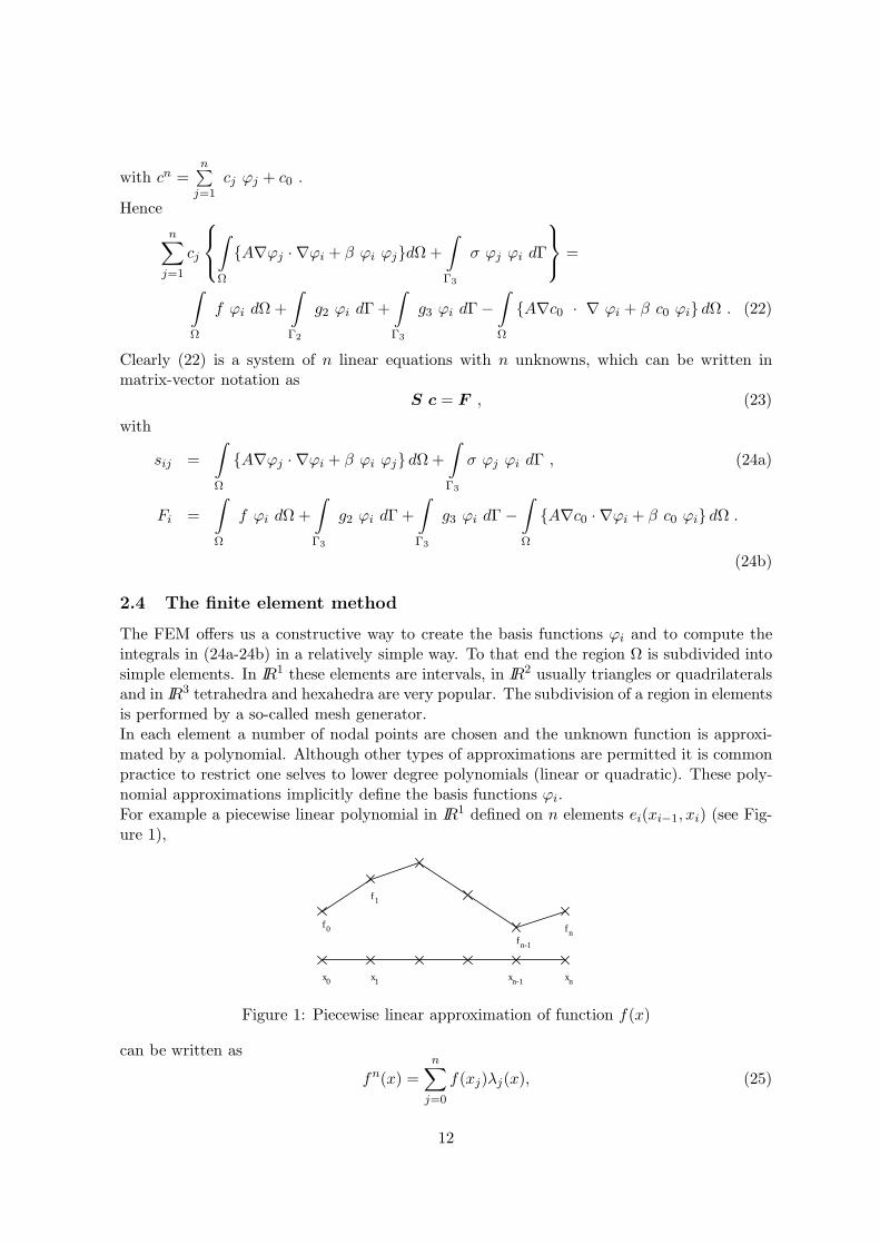
The FEM offers us a constructive way to create the basis functions ϕi and to compute theintegrals in (24a-24b) in a relatively simple way. To that end the region Ω is subdivided intosimple elements. In IR1 these elements are intervals, in IR2 usually triangles or quadrilateralsand in IR3 tetrahedra and hexahedra are very popular. The subdivision of a region in elementsis performed by a so-called mesh generator.In each element a number of nodal points are chosen and the unknown function is approxi-mated by a polynomial. Although other types of approximations are permitted it is commonpractice to restrict one selves to lower degree polynomials (linear or quadratic). These poly-nomial approximations implicitly define the basis functions ϕi.For example a piecewise linear polynomial in IR1 defined on n elements ei(xi−1, xi) (see Fig-ure 1),
n
x x x x
f
f
ff
0 1 n-1 n
0
1
n-1
Figure 1: Piecewise linear approximation of function f(x)
can be written as
fn(x) =
n∑
j=0
f(xj)λj(x), (25)
12
where λj(x) is defined as follows:
λj(x) is linear on each element,λj(xk) = δjk .
(26)
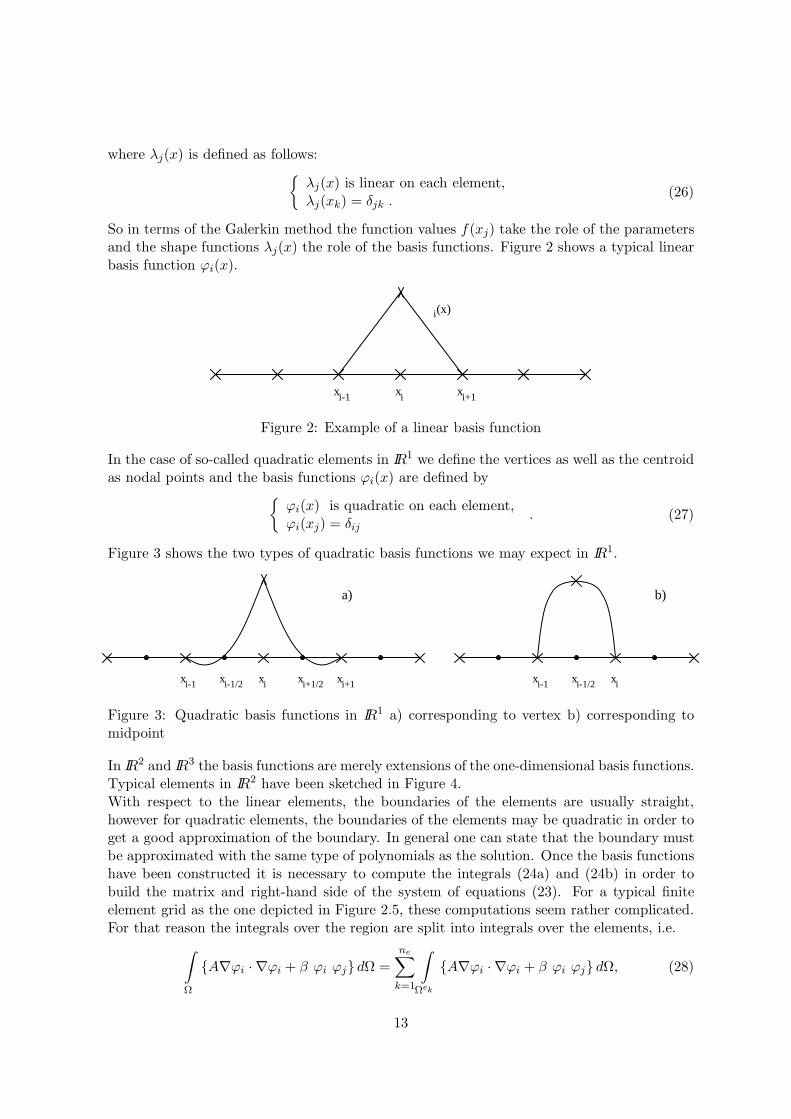
So in terms of the Galerkin method the function values f(xj) take the role of the parametersand the shape functions λj(x) the role of the basis functions. Figure 2 shows a typical linearbasis function ϕi(x).
i
x x x
j
i-1 i i+1
(x)
Figure 2: Example of a linear basis function
In the case of so-called quadratic elements in IR1 we define the vertices as well as the centroidas nodal points and the basis functions ϕi(x) are defined by
ϕi(x) is quadratic on each element,ϕi(xj) = δij
. (27)
Figure 3 shows the two types of quadratic basis functions we may expect in IR1.
i+1/2
b)a)
x x x x x x x xi-1 i-1/2 i i+1 i-1 i-1/2 i
Figure 3: Quadratic basis functions in IR1 a) corresponding to vertex b) corresponding tomidpoint
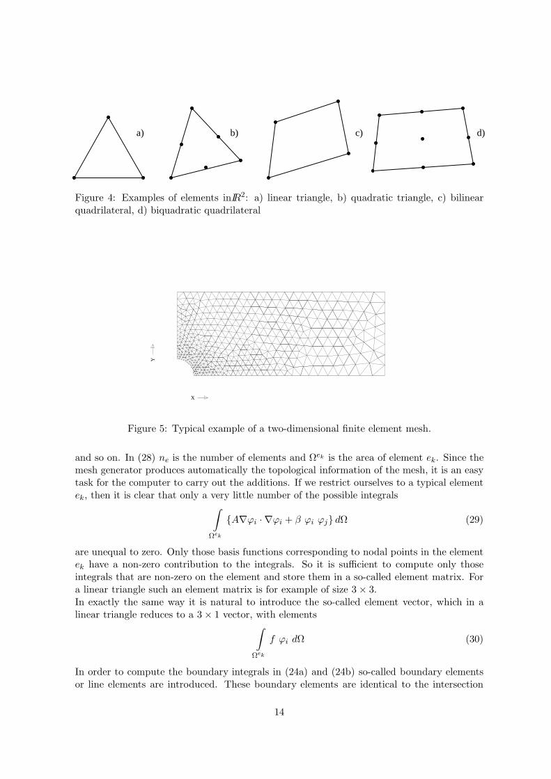
In IR2 and IR3 the basis functions are merely extensions of the one-dimensional basis functions.Typical elements in IR2 have been sketched in Figure 4.With respect to the linear elements, the boundaries of the elements are usually straight,however for quadratic elements, the boundaries of the elements may be quadratic in order toget a good approximation of the boundary. In general one can state that the boundary mustbe approximated with the same type of polynomials as the solution. Once the basis functionshave been constructed it is necessary to compute the integrals (24a) and (24b) in order tobuild the matrix and right-hand side of the system of equations (23). For a typical finiteelement grid as the one depicted in Figure 2.5, these computations seem rather complicated.For that reason the integrals over the region are split into integrals over the elements, i.e.
∫
Ω
A∇ϕi · ∇ϕi + β ϕi ϕj dΩ =ne∑
k=1
∫
Ωek
A∇ϕi · ∇ϕi + β ϕi ϕj dΩ, (28)
13
d)a) b) c)
Figure 4: Examples of elements inIR2: a) linear triangle, b) quadratic triangle, c) bilinearquadrilateral, d) biquadratic quadrilateral
X
Y
Figure 5: Typical example of a two-dimensional finite element mesh.
and so on. In (28) ne is the number of elements and Ωek is the area of element ek. Since themesh generator produces automatically the topological information of the mesh, it is an easytask for the computer to carry out the additions. If we restrict ourselves to a typical elementek, then it is clear that only a very little number of the possible integrals
∫
Ωek
A∇ϕi · ∇ϕi + β ϕi ϕj dΩ (29)
are unequal to zero. Only those basis functions corresponding to nodal points in the elementek have a non-zero contribution to the integrals. So it is sufficient to compute only thoseintegrals that are non-zero on the element and store them in a so-called element matrix. Fora linear triangle such an element matrix is for example of size 3× 3.In exactly the same way it is natural to introduce the so-called element vector, which in alinear triangle reduces to a 3× 1 vector, with elements
∫
Ωek
f ϕi dΩ (30)
In order to compute the boundary integrals in (24a) and (24b) so-called boundary elementsor line elements are introduced. These boundary elements are identical to the intersection
14
of the internal elements with the boundaries Γ2 and Γ3 and have no other purpose then toevaluate the boundary integrals. Here we have assumed that the boundary is identical to theouter boundary of the elements.Hence we get:
∫
Γ3
σ ϕi ϕj dΓ =nbe3∑
k=1
∫
Γek3
σ ϕi ϕj dΓ
∫
Γ2
g2 ϕi dΓ =nbe2∑
k=1
∫
Γek2
g2 ϕi dΓ
∫
Γ3
g3 ϕi dΓ =nbe3∑
k=1
∫
Γek3
g3ϕi dΓ
(31)
2.5 Computation of the element matrix and element vector
The evaluation of the system of equations (23), (24a-24b) is now reduced to the computation ofsome integrals over an arbitrary element. For the sake of simplicity we shall restrict ourselvesto IR2. As an example we consider the computation of the integral given by (29):
Sekij =
∫
Ωek
A∇ϕj · ∇ϕi + β ϕj ϕi dΩ (32)
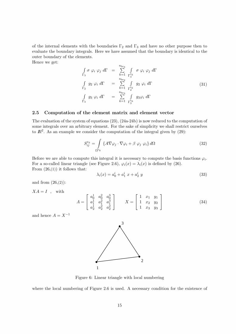
Before we are able to compute this integral it is necessary to compute the basis functions ϕi.For a so-called linear triangle (see Figure 2.6), ϕi(x) = λi(x) is defined by (26).From (26,(1)) it follows that:
λi(x) = ai0 + ai1 x+ ai2 y (33)
and from (26,(2)):
XA = I , with
A =
a10 a20 a30a11 a21 a31a12 a22 a22
X =
1 x1 y11 x2 y21 x3 y3
(34)
and hence A = X−1
3
1
2
Figure 6: Linear triangle with local numbering
where the local numbering of Figure 2.6 is used. A necessary condition for the existence of
15
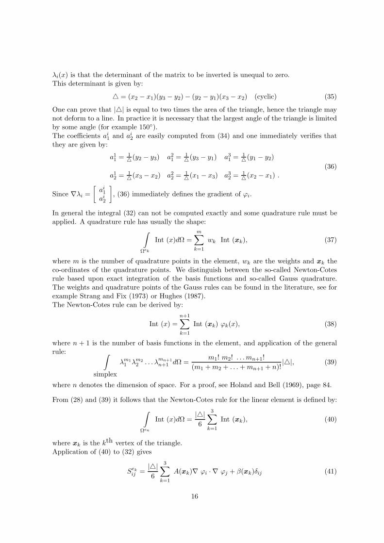
λi(x) is that the determinant of the matrix to be inverted is unequal to zero.This determinant is given by:
= (x2 − x1)(y3 − y2)− (y2 − y1)(x3 − x2) (cyclic) (35)
One can prove that || is equal to two times the area of the triangle, hence the triangle maynot deform to a line. In practice it is necessary that the largest angle of the triangle is limitedby some angle (for example 150).The coefficients ai1 and ai2 are easily computed from (34) and one immediately verifies thatthey are given by:
a11 =1(y2 − y3) a21 =
1(y3 − y1) a31 =
1(y1 − y2)
a12 =1(x3 − x2) a22 =
1(x1 − x3) a32 =
1(x2 − x1) .
(36)
Since ∇λi =[
ai1ai2
]
, (36) immediately defines the gradient of ϕi.
In general the integral (32) can not be computed exactly and some quadrature rule must beapplied. A quadrature rule has usually the shape:
∫
Ωek
Int (x)dΩ =
m∑
k=1
wk Int (xk), (37)
where m is the number of quadrature points in the element, wk are the weights and xk theco-ordinates of the quadrature points. We distinguish between the so-called Newton-Cotesrule based upon exact integration of the basis functions and so-called Gauss quadrature.The weights and quadrature points of the Gauss rules can be found in the literature, see forexample Strang and Fix (1973) or Hughes (1987).The Newton-Cotes rule can be derived by:
Int (x) =
n+1∑
k=1
Int (xk) ϕk(x), (38)
where n + 1 is the number of basis functions in the element, and application of the generalrule:
∫
simplex
λm1
1 λm2
2 . . . λmn+1
n+1 dΩ =m1! m2! . . . mn+1!
(m1 +m2 + . . .+mn+1 + n)!||, (39)
where n denotes the dimension of space. For a proof, see Holand and Bell (1969), page 84.
From (28) and (39) it follows that the Newton-Cotes rule for the linear element is defined by:
∫
Ωen
Int (x)dΩ =||6
3∑
k=1
Int (xk), (40)
where xk is the kth vertex of the triangle.Application of (40) to (32) gives
Sekij =
||6
3∑
k=1
A(xk)∇ ϕi · ∇ ϕj + β(xk)δij (41)
16
In the same way (30) may be approximated by
f eki =||6f(xi) . (42)
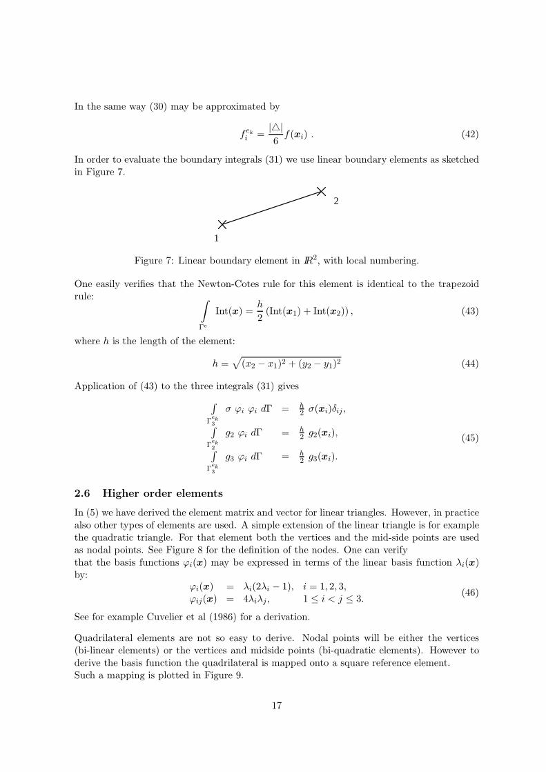
In order to evaluate the boundary integrals (31) we use linear boundary elements as sketchedin Figure 7.
1
2
Figure 7: Linear boundary element in IR2, with local numbering.
One easily verifies that the Newton-Cotes rule for this element is identical to the trapezoidrule:
∫
Γe
Int(x) =h
2(Int(x1) + Int(x2)) , (43)
where h is the length of the element:
h =√
(x2 − x1)2 + (y2 − y1)2 (44)
Application of (43) to the three integrals (31) gives
∫
Γek3
σ ϕi ϕi dΓ = h2 σ(xi)δij ,
∫
Γek2
g2 ϕi dΓ = h2 g2(xi),
∫
Γek3
g3 ϕi dΓ = h2 g3(xi).
(45)
2.6 Higher order elements
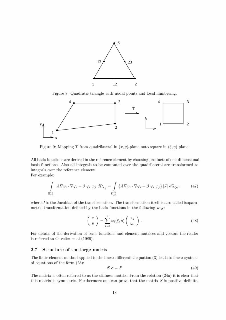
In (5) we have derived the element matrix and vector for linear triangles. However, in practicealso other types of elements are used. A simple extension of the linear triangle is for examplethe quadratic triangle. For that element both the vertices and the mid-side points are usedas nodal points. See Figure 8 for the definition of the nodes. One can verifythat the basis functions ϕi(x) may be expressed in terms of the linear basis function λi(x)by:
ϕi(x) = λi(2λi − 1), i = 1, 2, 3,ϕij(x) = 4λiλj , 1 ≤ i < j ≤ 3.
(46)
See for example Cuvelier et al (1986) for a derivation.
Quadrilateral elements are not so easy to derive. Nodal points will be either the vertices(bi-linear elements) or the vertices and midside points (bi-quadratic elements). However toderive the basis function the quadrilateral is mapped onto a square reference element.Such a mapping is plotted in Figure 9.
17
3
1 12 2
2313
Figure 8: Quadratic triangle with nodal points and local numbering.
2
T
34
y
1x
1 2
34
h
x
Figure 9: Mapping T from quadrilateral in (x, y)-plane onto square in (ξ, η) plane.
All basis functions are derived in the reference element by choosing products of one-dimensionalbasis functions. Also all integrals to be computed over the quadrilateral are transformed tointegrals over the reference element.For example:
∫
Ωekxy
A∇ϕi · ∇ϕi + β ϕi ϕj dΩxy =
∫
Ωekξη
A∇ϕi · ∇ϕi + β ϕi ϕj |J | dΩξη , (47)
where J is the Jacobian of the transformation. The transformation itself is a so-called isopara-metric transformation defined by the basis functions in the following way:
(
xy
)
=
4∑
k=1
ϕi(ξ, η)
(
xkyk
)
. (48)
For details of the derivation of basis functions and element matrices and vectors the readeris referred to Cuvelier et al (1986).
2.7 Structure of the large matrix
The finite element method applied to the linear differential equation (3) leads to linear systemsof equations of the form (23):
S c = F (49)
The matrix is often referred to as the stiffness matrix. From the relation (24a) it is clear thatthis matrix is symmetric. Furthermore one can prove that the matrix S is positive definite,
18
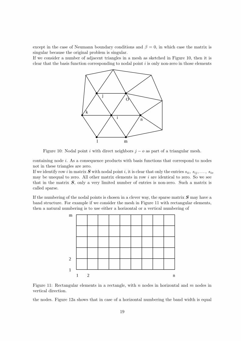
except in the case of Neumann boundary conditions and β = 0, in which case the matrix issingular because the original problem is singular.If we consider a number of adjacent triangles in a mesh as sketched in Figure 10, then it isclear that the basis function corresponding to nodal point i is only non-zero in those elements
l
i n
m
k
jO
Figure 10: Nodal point i with direct neighbors j − o as part of a triangular mesh.
containing node i. As a consequence products with basis functions that correspond to nodesnot in these triangles are zero.If we identify row i in matrix S with nodal point i, it is clear that only the entries sii, sij , . . . , siomay be unequal to zero. All other matrix elements in row i are identical to zero. So we seethat in the matrix S, only a very limited number of entries is non-zero. Such a matrix iscalled sparse.
If the numbering of the nodal points is chosen in a clever way, the sparse matrix S may have aband structure. For example if we consider the mesh in Figure 11 with rectangular elements,then a natural numbering is to use either a horizontal or a vertical numbering of
m
1 2 n1
2
Figure 11: Rectangular elements in a rectangle, with n nodes in horizontal and m nodes invertical direction.
the nodes. Figure 12a shows that in case of a horizontal numbering the band width is equal
19
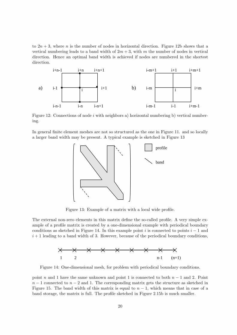
to 2n + 3, where n is the number of nodes in horizontal direction. Figure 12b shows that avertical numbering leads to a band width of 2m+ 3, with m the number of nodes in verticaldirection. Hence an optimal band width is achieved if nodes are numbered in the shortestdirection.
b)a)
i+1 i+m+1
i-m i
i-m+1
i-m-1 i-1 i+m-1
i+m
i+n i+n+1
i
i-n i-n+1
i+1i-1
i-n-1
i+n-1
Figure 12: Connections of node i with neighbors a) horizontal numbering b) vertical number-ing.
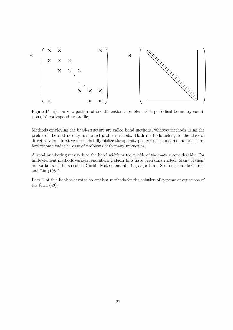
In general finite element meshes are not so structured as the one in Figure 11. and so locallya larger band width may be present. A typical example is sketched in Figure 13
band
profile
Figure 13: Example of a matrix with a local wide profile.
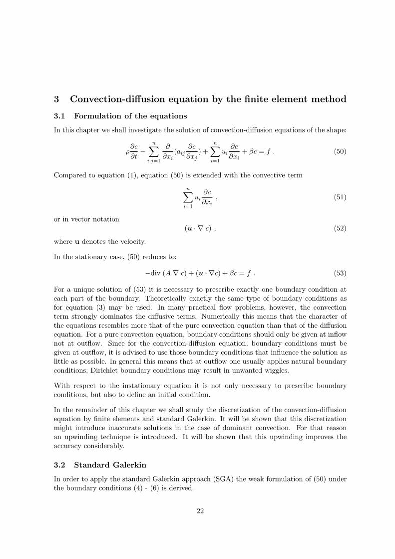
The external non-zero elements in this matrix define the so-called profile. A very simple ex-ample of a profile matrix is created by a one-dimensional example with periodical boundaryconditions as sketched in Figure 14. In this example point i is connected to points i− 1 andi+ 1 leading to a band width of 3. However, because of the periodical boundary conditions,
(n=1)1 2 n-1
Figure 14: One-dimensional mesh, for problem with periodical boundary conditions.
point n and 1 have the same unknown and point 1 is connected to both n − 1 and 2. Pointn− 1 connected to n− 2 and 1. The corresponding matrix gets the structure as sketched inFigure 15. The band width of this matrix is equal to n − 1, which means that in case of aband storage, the matrix is full. The profile sketched in Figure 2.15b is much smaller.
20
a) b)
Figure 15: a) non-zero pattern of one-dimensional problem with periodical boundary condi-tions, b) corresponding profile.
Methods employing the band-structure are called band methods, whereas methods using theprofile of the matrix only are called profile methods. Both methods belong to the class ofdirect solvers. Iterative methods fully utilize the sparsity pattern of the matrix and are there-fore recommended in case of problems with many unknowns.
A good numbering may reduce the band width or the profile of the matrix considerably. Forfinite element methods various renumbering algorithms have been constructed. Many of themare variants of the so-called Cuthill-Mckee renumbering algorithm. See for example Georgeand Liu (1981).
Part II of this book is devoted to efficient methods for the solution of systems of equations ofthe form (49).
21
3 Convection-diffusion equation by the finite element method
3.1 Formulation of the equations
In this chapter we shall investigate the solution of convection-diffusion equations of the shape:
ρ∂c
∂t−
n∑
i,j=1
∂
∂xi(aij
∂c
∂xj) +
n∑
i=1
ui∂c
∂xi+ βc = f . (50)
Compared to equation (1), equation (50) is extended with the convective term
n∑
i=1
ui∂c
∂xi, (51)
or in vector notation(u · ∇ c) , (52)
where u denotes the velocity.
In the stationary case, (50) reduces to:
−div (A ∇ c) + (u · ∇c) + βc = f . (53)
For a unique solution of (53) it is necessary to prescribe exactly one boundary condition ateach part of the boundary. Theoretically exactly the same type of boundary conditions asfor equation (3) may be used. In many practical flow problems, however, the convectionterm strongly dominates the diffusive terms. Numerically this means that the character ofthe equations resembles more that of the pure convection equation than that of the diffusionequation. For a pure convection equation, boundary conditions should only be given at inflownot at outflow. Since for the convection-diffusion equation, boundary conditions must begiven at outflow, it is advised to use those boundary conditions that influence the solution aslittle as possible. In general this means that at outflow one usually applies natural boundaryconditions; Dirichlet boundary conditions may result in unwanted wiggles.
With respect to the instationary equation it is not only necessary to prescribe boundaryconditions, but also to define an initial condition.
In the remainder of this chapter we shall study the discretization of the convection-diffusionequation by finite elements and standard Galerkin. It will be shown that this discretizationmight introduce inaccurate solutions in the case of dominant convection. For that reasonan upwinding technique is introduced. It will be shown that this upwinding improves theaccuracy considerably.
3.2 Standard Galerkin
In order to apply the standard Galerkin approach (SGA) the weak formulation of (50) underthe boundary conditions (4) - (6) is derived.
22
Multiplication of (50) by a time-independent test function v and integration over the domainyields:
∫
Ω
ρ∂c
∂tvdΩ+
∫
Ω
−div (A∇c) + (u · ∇c) + βcvdΩ =
∫
Ω
fvdΩ . (54)
After application of the Gauss divergence theorem, which results in relation (12), (54) can bewritten as
∫
Ω
ρ∂c
∂tvdΩ+
∫
Ω
(A∇c · ∇v + βcv + u · ∇c)vdΩ −∫
Γ
vA∇c · ndΓ =
∫
Ω
fvdΩ . (55)
Substitution of the boundary conditions in the same way as is performed in Chapter 2 resultsin the weak formulation:
Find c(x, t) with c(x, 0) given and c|Γ1= g1 such that
∫
Ω
ρ∂c
∂tvdΩ +
∫
Ω
(A∇c · ∇v) + u · ∇cv + βcvdΩ +
∫
Γ3
σcvdΓ =
∫
Ω
fvdΩ+
∫
Γ2
g2vdΓ +
∫
Γ3
g3vdΓ , (56)
for all functions v(x) satisfying v|Γ1= 0 .
In the SGA the weak form (56) is approximated by a finite dimensional subspace. To thatend we define time-independent basis functions in exactly the same way as for the potentialproblem. The solution c is approximated by a linear combination of the basis functions:
ch(x, t) =n∑
j=1
cj(t)ϕj(x) + c0(x, t) . (57)
The basis functions ϕj(x) and the function c0(x, t) must satisfy the same requirements as inChapter 2, i.e. (18) and (19) are still necessary.For the test functions v(x) again the basis functions ϕi(x) (i = 1, 2, ..., n) are substituted. Sofinally we arrive at the Galerkin formulation:
n∑
j=1
∂cj∂t
∫
Ω
ϕiϕjdΩ+n∑
j=1
cj∫
Ω
[(A∇ϕj · ∇ϕi) + (u · ∇ϕj)ϕi + βϕiϕj ]dΩ
+
∫
Γ3
σϕiϕjdΓ =
∫
Ω
fϕidΩ+
∫
Γ2
g2ϕidΓ +
∫
Γ3
g3ϕidΓ (58)
−∫
Ω
(A∇c0 · ∇ϕi) + βc0ϕi + (u · ∇c0)ϕidΩ −∫
Ω
∂c0∂t
ϕidΩ , i = 1(1)n .
Clearly (58) forms a system of n linear ordinary differential equations with n unknowns, whichcan be written in matrix-vector notation as
Mc+ Sc = F , (59)
23
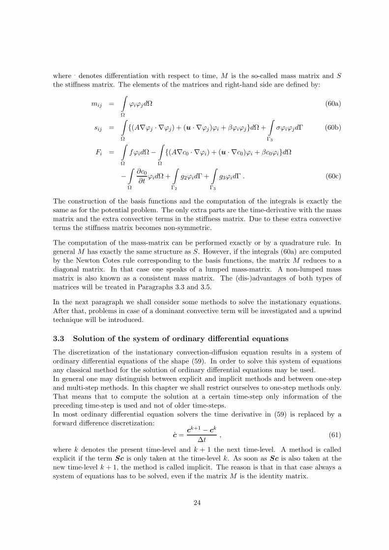
where . denotes differentiation with respect to time, M is the so-called mass matrix and Sthe stiffness matrix. The elements of the matrices and right-hand side are defined by:
mij =
∫
Ω
ϕiϕjdΩ (60a)
sij =
∫
Ω
(A∇ϕj · ∇ϕj) + (u · ∇ϕj)ϕi + βϕiϕjdΩ+
∫
Γ3
σϕiϕjdΓ (60b)
Fi =
∫
Ω
fϕidΩ−∫
Ω
(A∇c0 · ∇ϕi) + (u · ∇c0)ϕi + βc0ϕidΩ
−∫
Ω
∂c0∂t
ϕidΩ+
∫
Γ2
g2ϕidΓ +
∫
Γ3
g3ϕidΓ . (60c)
The construction of the basis functions and the computation of the integrals is exactly thesame as for the potential problem. The only extra parts are the time-derivative with the massmatrix and the extra convective terms in the stiffness matrix. Due to these extra convectiveterms the stiffness matrix becomes non-symmetric.
The computation of the mass-matrix can be performed exactly or by a quadrature rule. Ingeneral M has exactly the same structure as S. However, if the integrals (60a) are computedby the Newton Cotes rule corresponding to the basis functions, the matrix M reduces to adiagonal matrix. In that case one speaks of a lumped mass-matrix. A non-lumped massmatrix is also known as a consistent mass matrix. The (dis-)advantages of both types ofmatrices will be treated in Paragraphs 3.3 and 3.5.
In the next paragraph we shall consider some methods to solve the instationary equations.After that, problems in case of a dominant convective term will be investigated and a upwindtechnique will be introduced.
3.3 Solution of the system of ordinary differential equations
The discretization of the instationary convection-diffusion equation results in a system ofordinary differential equations of the shape (59). In order to solve this system of equationsany classical method for the solution of ordinary differential equations may be used.In general one may distinguish between explicit and implicit methods and between one-stepand multi-step methods. In this chapter we shall restrict ourselves to one-step methods only.That means that to compute the solution at a certain time-step only information of thepreceding time-step is used and not of older time-steps.In most ordinary differential equation solvers the time derivative in (59) is replaced by aforward difference discretization:
c =ck+1 − ck
∆t, (61)
where k denotes the present time-level and k + 1 the next time-level. A method is calledexplicit if the term Sc is only taken at the time-level k. As soon as Sc is also taken at thenew time-level k + 1, the method is called implicit. The reason is that in that case always asystem of equations has to be solved, even if the matrix M is the identity matrix.
24
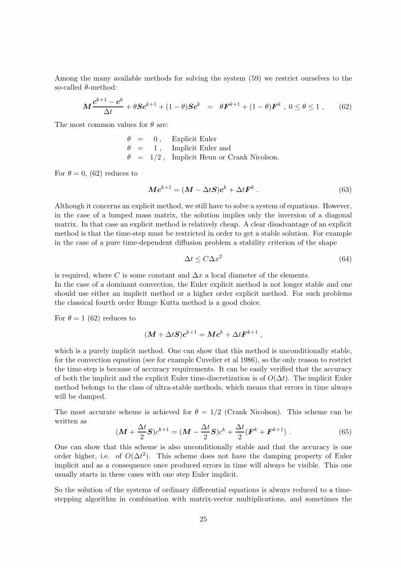
Among the many available methods for solving the system (59) we restrict ourselves to theso-called θ-method:
Mck+1 − ck
∆t+ θSck+1 + (1− θ)Sck = θF k+1 + (1− θ)F k , 0 ≤ θ ≤ 1 , (62)
The most common values for θ are:
θ = 0 , Explicit Eulerθ = 1 , Implicit Euler andθ = 1/2 , Implicit Heun or Crank Nicolson.
For θ = 0, (62) reduces to
Mck+1 = (M −∆tS)ck +∆tF k . (63)
Although it concerns an explicit method, we still have to solve a system of equations. However,in the case of a lumped mass matrix, the solution implies only the inversion of a diagonalmatrix. In that case an explicit method is relatively cheap. A clear disadvantage of an explicitmethod is that the time-step must be restricted in order to get a stable solution. For examplein the case of a pure time-dependent diffusion problem a stability criterion of the shape
∆t ≤ C∆x2 (64)
is required, where C is some constant and ∆x a local diameter of the elements.In the case of a dominant convection, the Euler explicit method is not longer stable and oneshould use either an implicit method or a higher order explicit method. For such problemsthe classical fourth order Runge Kutta method is a good choice.
For θ = 1 (62) reduces to
(M +∆tS)ck+1 = Mck +∆tF k+1 ,
which is a purely implicit method. One can show that this method is unconditionally stable,for the convection equation (see for example Cuvelier et al 1986), so the only reason to restrictthe time-step is because of accuracy requirements. It can be easily verified that the accuracyof both the implicit and the explicit Euler time-discretization is of O(∆t). The implicit Eulermethod belongs to the class of ultra-stable methods, which means that errors in time alwayswill be damped.
The most accurate scheme is achieved for θ = 1/2 (Crank Nicolson). This scheme can bewritten as
(M +∆t
2S)ck+1 = (M − ∆t
2S)ck +
∆t
2(F k + F k+1) . (65)
One can show that this scheme is also unconditionally stable and that the accuracy is oneorder higher, i.e. of O(∆t2). This scheme does not have the damping property of Eulerimplicit and as a consequence once produced errors in time will always be visible. This oneusually starts in these cases with one step Euler implicit.
So the solution of the systems of ordinary differential equations is always reduced to a time-stepping algorithm in combination with matrix-vector multiplications, and sometimes the
25
solution of a system of linear equations.
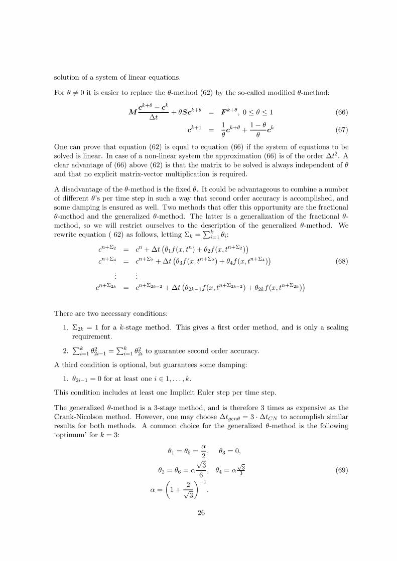
For θ 6= 0 it is easier to replace the θ-method (62) by the so-called modified θ-method:
Mck+θ − ck
∆t+ θSck+θ = F k+θ, 0 ≤ θ ≤ 1 (66)
ck+1 =1
θck+θ +
1− θ
θck (67)
One can prove that equation (62) is equal to equation (66) if the system of equations to besolved is linear. In case of a non-linear system the approximation (66) is of the order ∆t2. Aclear advantage of (66) above (62) is that the matrix to be solved is always independent of θand that no explicit matrix-vector multiplication is required.
A disadvantage of the θ-method is the fixed θ. It could be advantageous to combine a numberof different θ’s per time step in such a way that second order accuracy is accomplished, andsome damping is ensured as well. Two methods that offer this opportunity are the fractionalθ-method and the generalized θ-method. The latter is a generalization of the fractional θ-method, so we will restrict ourselves to the description of the generalized θ-method. Werewrite equation ( 62) as follows, letting Σk =
∑ki=1 θi:
cn+Σ2 = cn +∆t(
θ1f(x, tn) + θ2f(x, t
n+Σ2))
cn+Σ4 = cn+Σ2 +∆t(
θ3f(x, tn+Σ2) + θ4f(x, t
n+Σ4))
(68)
......
cn+Σ2k = cn+Σ2k−2 +∆t(
θ2k−1f(x, tn+Σ2k−2) + θ2kf(x, t
n+Σ2k))
There are two necessary conditions:
1. Σ2k = 1 for a k-stage method. This gives a first order method, and is only a scalingrequirement.
2.∑k
i=1 θ22i−1 =
∑ki=1 θ
22i to guarantee second order accuracy.
A third condition is optional, but guarantees some damping:
1. θ2i−1 = 0 for at least one i ∈ 1, . . . , k.
This condition includes at least one Implicit Euler step per time step.
The generalized θ-method is a 3-stage method, and is therefore 3 times as expensive as theCrank-Nicolson method. However, one may choose ∆tgenθ = 3 ·∆tCN to accomplish similarresults for both methods. A common choice for the generalized θ-method is the following‘optimum’ for k = 3:
θ1 = θ5 =α
2, θ3 = 0,
θ2 = θ6 = α
√3
6, θ4 = α
√33 (69)
α =
(
1 +2√3
)−1
.
26
A common choice for the fractional θ-method is the following:
θ1 = θ5 = βθ, θ3 = α(1− 2θ),
θ2 = θ6 = αθ, θ4 = β(1− 2θ), (70)
α =1− 2θ
1− θ, β = θ
1−θ,
θ = 1− 1
2
√2.
3.4 Accuracy aspects of the SGA
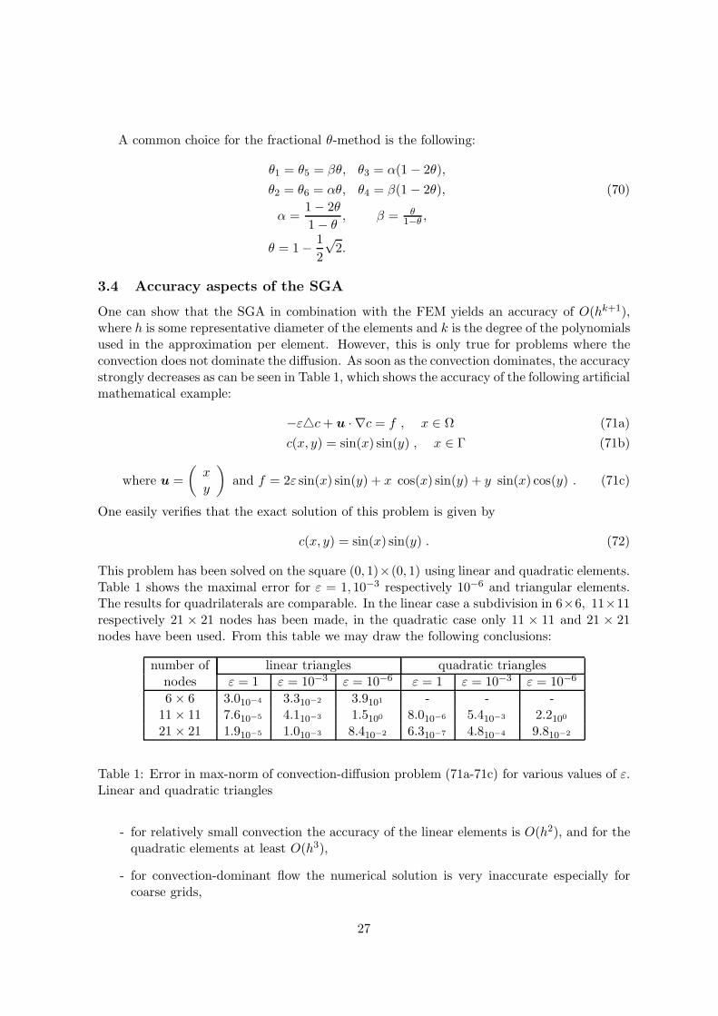
One can show that the SGA in combination with the FEM yields an accuracy of O(hk+1),where h is some representative diameter of the elements and k is the degree of the polynomialsused in the approximation per element. However, this is only true for problems where theconvection does not dominate the diffusion. As soon as the convection dominates, the accuracystrongly decreases as can be seen in Table 1, which shows the accuracy of the following artificialmathematical example:
−εc+ u · ∇c = f , x ∈ Ω (71a)
c(x, y) = sin(x) sin(y) , x ∈ Γ (71b)
where u =
(
xy
)
and f = 2ε sin(x) sin(y) + x cos(x) sin(y) + y sin(x) cos(y) . (71c)
One easily verifies that the exact solution of this problem is given by
c(x, y) = sin(x) sin(y) . (72)
This problem has been solved on the square (0, 1)×(0, 1) using linear and quadratic elements.Table 1 shows the maximal error for ε = 1, 10−3 respectively 10−6 and triangular elements.The results for quadrilaterals are comparable. In the linear case a subdivision in 6×6, 11×11respectively 21 × 21 nodes has been made, in the quadratic case only 11 × 11 and 21 × 21nodes have been used. From this table we may draw the following conclusions:
number of linear triangles quadratic trianglesnodes ε = 1 ε = 10−3 ε = 10−6 ε = 1 ε = 10−3 ε = 10−6
6× 6 3.010−4 3.310−2 3.9101 - - -11× 11 7.610−5 4.110−3 1.5100 8.010−6 5.410−3 2.210021× 21 1.910−5 1.010−3 8.410−2 6.310−7 4.810−4 9.810−2
Table 1: Error in max-norm of convection-diffusion problem (71a-71c) for various values of ε.Linear and quadratic triangles
- for relatively small convection the accuracy of the linear elements is O(h2), and for thequadratic elements at least O(h3),
- for convection-dominant flow the numerical solution is very inaccurate especially forcoarse grids,
27
- the use of quadratic elements makes only sense for problems with small convection.
Remark: the conclusions are based on an example with a very smooth solution. For prob-lems with steep gradients the conclusion may be different, especially for the quadraticelements, in which cases the O(h3) cannot be expected anymore.
The most important part of the conclusion is that SGA is not a good method for convection-dominant flows. This conclusion is also motivated by the following less trivial problem.
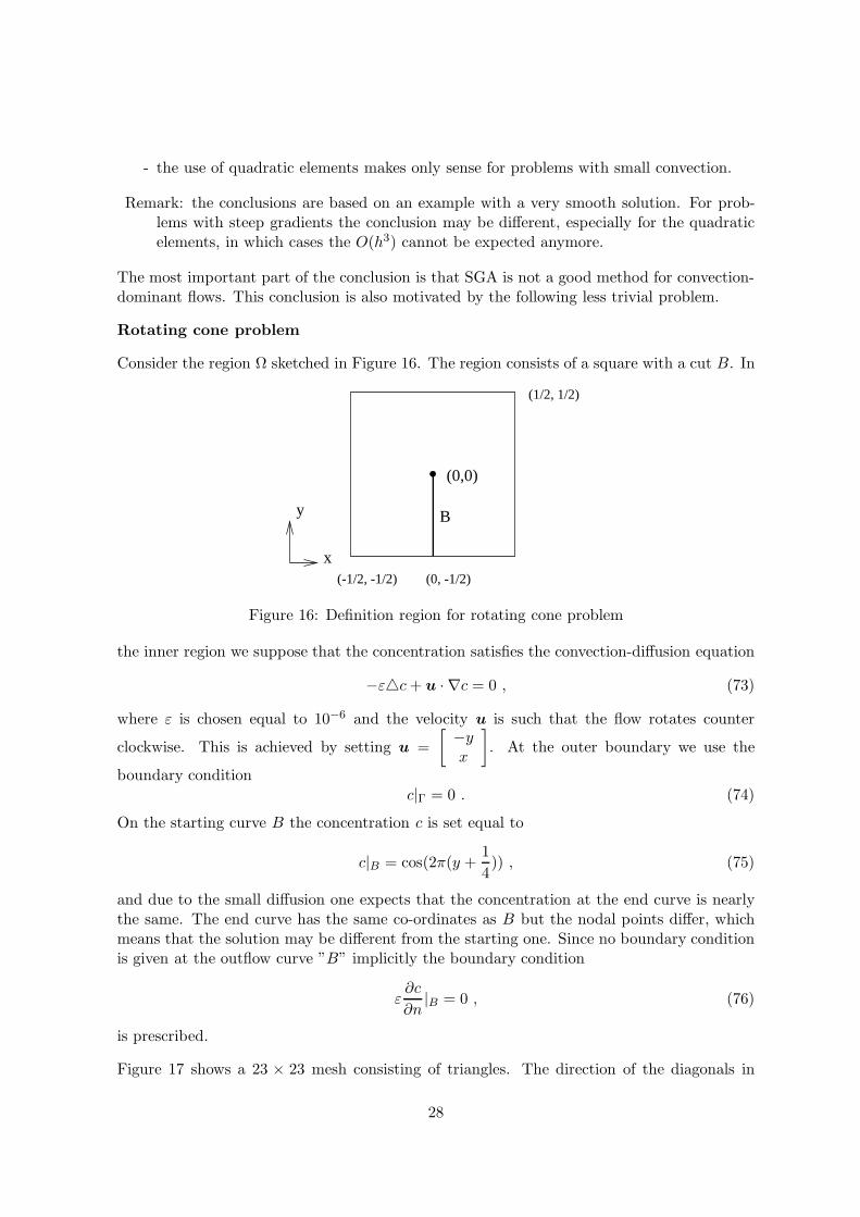
Rotating cone problem
Consider the region Ω sketched in Figure 16. The region consists of a square with a cut B. In
W(0,0)
y B
(-1/2, -1/2)
(1/2, 1/2)
(0, -1/2)
x
Figure 16: Definition region for rotating cone problem
the inner region we suppose that the concentration satisfies the convection-diffusion equation
−εc+ u · ∇c = 0 , (73)
where ε is chosen equal to 10−6 and the velocity u is such that the flow rotates counter
clockwise. This is achieved by setting u =
[
−yx
]
. At the outer boundary we use the
boundary conditionc|Γ = 0 . (74)
On the starting curve B the concentration c is set equal to
c|B = cos(2π(y +1
4)) , (75)
and due to the small diffusion one expects that the concentration at the end curve is nearlythe same. The end curve has the same co-ordinates as B but the nodal points differ, whichmeans that the solution may be different from the starting one. Since no boundary conditionis given at the outflow curve ”B” implicitly the boundary condition
ε∂c
∂n|B = 0 , (76)
is prescribed.
Figure 17 shows a 23 × 23 mesh consisting of triangles. The direction of the diagonals in
28
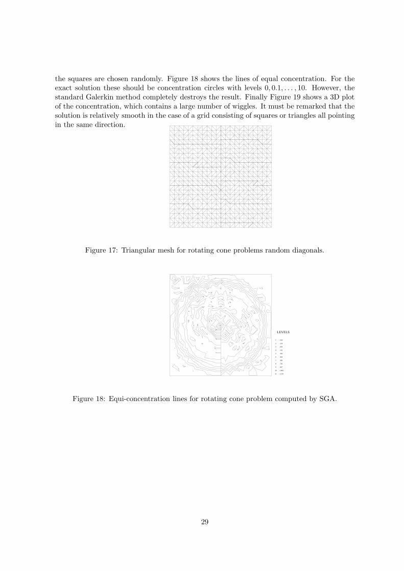
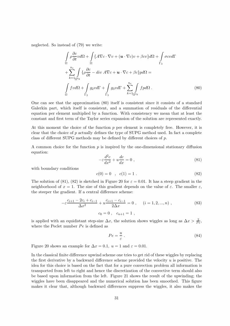
the squares are chosen randomly. Figure 18 shows the lines of equal concentration. For theexact solution these should be concentration circles with levels 0, 0.1, . . . , 10. However, thestandard Galerkin method completely destroys the result. Finally Figure 19 shows a 3D plotof the concentration, which contains a large number of wiggles. It must be remarked that thesolution is relatively smooth in the case of a grid consisting of squares or triangles all pointingin the same direction.
Figure 17: Triangular mesh for rotating cone problems random diagonals.
1
2
2
2
2
2
2
2
2 22
2
2
2
3
3
3
3
3
3
3
3
4
4
45
5
5
5
5
6
6
6
6
7
7
7
7
8
8
8
8
8
8
8
8
9
9
9
9
9
9
9
9
9
9
9
9 9
99
9
9
9
9
9
9
10
10
10
10
10
10 10
10
1010
10
1010
10
10
10
10
10
10
11
LEVELS
1 -.263
2 -.122
3 .019
4 .161
5 .302
6 .443
7 .585
8 .726
9 .867
10 1.009
11 1.150
Figure 18: Equi-concentration lines for rotating cone problem computed by SGA.
29
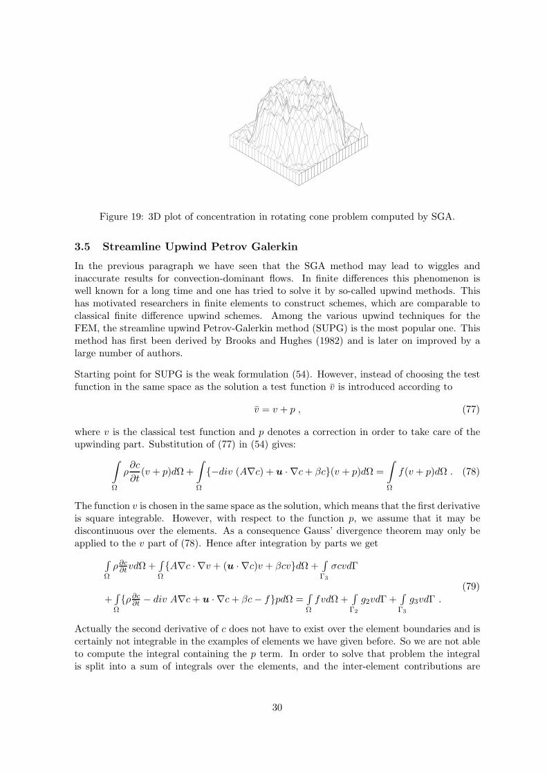
Figure 19: 3D plot of concentration in rotating cone problem computed by SGA.
3.5 Streamline Upwind Petrov Galerkin
In the previous paragraph we have seen that the SGA method may lead to wiggles andinaccurate results for convection-dominant flows. In finite differences this phenomenon iswell known for a long time and one has tried to solve it by so-called upwind methods. Thishas motivated researchers in finite elements to construct schemes, which are comparable toclassical finite difference upwind schemes. Among the various upwind techniques for theFEM, the streamline upwind Petrov-Galerkin method (SUPG) is the most popular one. Thismethod has first been derived by Brooks and Hughes (1982) and is later on improved by alarge number of authors.
Starting point for SUPG is the weak formulation (54). However, instead of choosing the testfunction in the same space as the solution a test function v is introduced according to
v = v + p , (77)
where v is the classical test function and p denotes a correction in order to take care of theupwinding part. Substitution of (77) in (54) gives:
∫
Ω
ρ∂c
∂t(v + p)dΩ+
∫
Ω
−div (A∇c) + u · ∇c+ βc(v + p)dΩ =
∫
Ω
f(v + p)dΩ . (78)
The function v is chosen in the same space as the solution, which means that the first derivativeis square integrable. However, with respect to the function p, we assume that it may bediscontinuous over the elements. As a consequence Gauss’ divergence theorem may only beapplied to the v part of (78). Hence after integration by parts we get
∫
Ω
ρ∂c∂tvdΩ+
∫
Ω
A∇c · ∇v + (u · ∇c)v + βcvdΩ +∫
Γ3
σcvdΓ
+∫
Ω
ρ∂c∂t
− div A∇c+ u · ∇c+ βc− fpdΩ =∫
Ω
fvdΩ+∫
Γ2
g2vdΓ +∫
Γ3
g3vdΓ .
(79)
Actually the second derivative of c does not have to exist over the element boundaries and iscertainly not integrable in the examples of elements we have given before. So we are not ableto compute the integral containing the p term. In order to solve that problem the integralis split into a sum of integrals over the elements, and the inter-element contributions are
30
neglected. So instead of (79) we write:
∫
Ω
ρ∂c
∂tvdΩ+
∫
Ω
A∇c · ∇v + (u · ∇c)v + βcvdΩ +
∫
Γ3
σcvdΓ
+
ne∑
k=1
∫
Ωek
ρ∂c∂t
− div A∇c+ u · ∇c+ βcpdΩ =
∫
Ω
fvdΩ+
∫
Γ2
g2vdΓ +
∫
Γ3
g3vdΓ +
ne∑
k=1
∫
Ωek
fpdΩ . (80)
One can see that the approximation (80) itself is consistent since it consists of a standardGalerkin part, which itself is consistent, and a summation of residuals of the differentialequation per element multiplied by a function. With consistency we mean that at least theconstant and first term of the Taylor series expansion of the solution are represented exactly.
At this moment the choice of the function p per element is completely free. However, it isclear that the choice of p actually defines the type of SUPG method used. In fact a completeclass of different SUPG methods may be defined by different choices of p.
A common choice for the function p is inspired by the one-dimensional stationary diffusionequation:
−ε d2c
dx2+ u
dc
dx= 0 , (81)
with boundary conditionsc(0) = 0 , c(1) = 1 . (82)
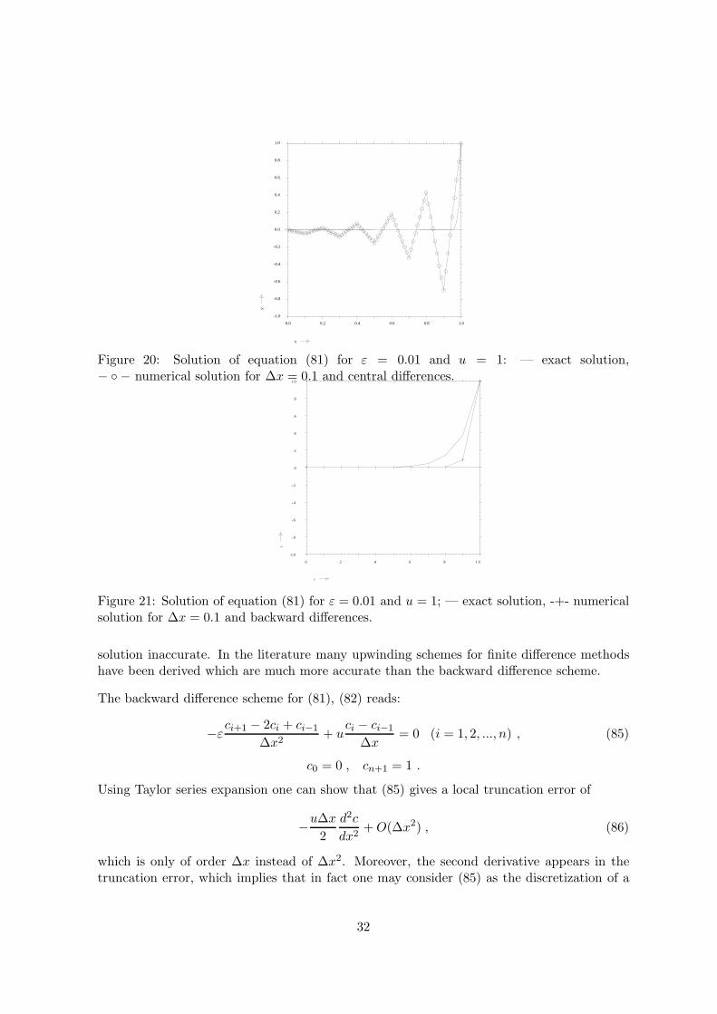
The solution of (81), (82) is sketched in Figure 20 for ε = 0.01. It has a steep gradient in theneighborhood of x = 1. The size of this gradient depends on the value of ε. The smaller ε,the steeper the gradient. If a central difference scheme:
−εci+1 − 2ci + ci−1
∆x2+ u
ci+1 − ci−1
2∆x= 0 , (i = 1, 2, ..., n) , (83)
c0 = 0 , cn+1 = 1 ,
is applied with an equidistant step-size ∆x, the solution shows wiggles as long as ∆x > 2Pe
,where the Peclet number Pe is defined as
Pe =u
ε. (84)
Figure 20 shows an example for ∆x = 0.1, u = 1 and ε = 0.01.
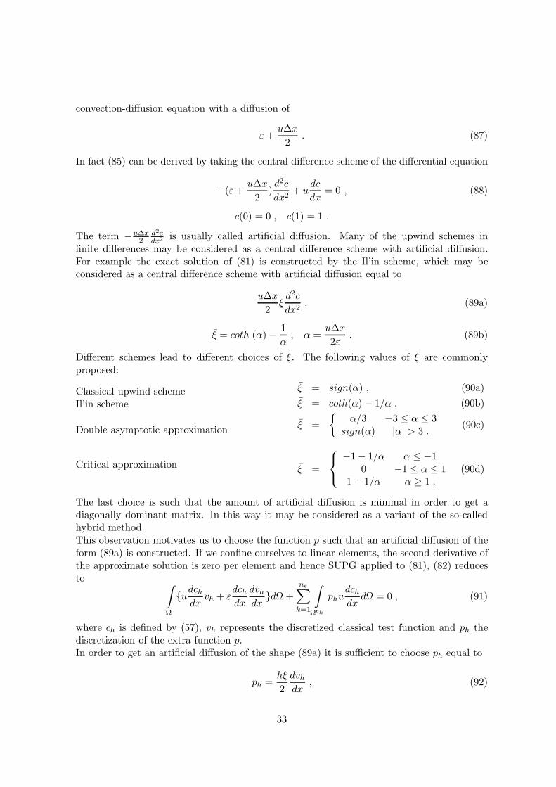
In the classical finite difference upwind scheme one tries to get rid of these wiggles by replacingthe first derivative by a backward difference scheme provided the velocity u is positive. Theidea for this choice is based on the fact that for a pure convection problem all information istransported from left to right and hence the discretization of the convective term should alsobe based upon information from the left. Figure 21 shows the result of the upwinding; thewiggles have been disappeared and the numerical solution has been smoothed. This figuremakes it clear that, although backward differences suppress the wiggles, it also makes the
31
0.0 0.2 0.4 0.6 0.8 1.0
-1.0
-0.8
-0.6
-0.4
-0.2
0.0
0.2
0.4
0.6
0.8
1.0
x
y
Figure 20: Solution of equation (81) for ε = 0.01 and u = 1: — exact solution,− − numerical solution for ∆x = 0.1 and central differences.
.0 .2 .4 .6 .8 1.0
-1.0
-.8
-.6
-.4
-.2
.0
.2
.4
.6
.8
1.0
x
y
Figure 21: Solution of equation (81) for ε = 0.01 and u = 1; — exact solution, -+- numericalsolution for ∆x = 0.1 and backward differences.
solution inaccurate. In the literature many upwinding schemes for finite difference methodshave been derived which are much more accurate than the backward difference scheme.
The backward difference scheme for (81), (82) reads:
−εci+1 − 2ci + ci−1
∆x2+ u
ci − ci−1
∆x= 0 (i = 1, 2, ..., n) , (85)
c0 = 0 , cn+1 = 1 .
Using Taylor series expansion one can show that (85) gives a local truncation error of
−u∆x2
d2c
dx2+O(∆x2) , (86)
which is only of order ∆x instead of ∆x2. Moreover, the second derivative appears in thetruncation error, which implies that in fact one may consider (85) as the discretization of a
32
convection-diffusion equation with a diffusion of
ε+u∆x
2. (87)
In fact (85) can be derived by taking the central difference scheme of the differential equation
−(ε+u∆x
2)d2c
dx2+ u
dc
dx= 0 , (88)
c(0) = 0 , c(1) = 1 .
The term −u∆x2
d2cdx2 is usually called artificial diffusion. Many of the upwind schemes in
finite differences may be considered as a central difference scheme with artificial diffusion.For example the exact solution of (81) is constructed by the Il’in scheme, which may beconsidered as a central difference scheme with artificial diffusion equal to
u∆x
2ξd2c
dx2, (89a)
ξ = coth (α)− 1
α, α =
u∆x
2ε. (89b)
Different schemes lead to different choices of ξ. The following values of ξ are commonlyproposed:
Classical upwind schemeIl’in scheme
Double asymptotic approximation
Critical approximation
ξ = sign(α) , (90a)
ξ = coth(α) − 1/α . (90b)
ξ =
α/3 −3 ≤ α ≤ 3sign(α) |α| > 3 .
(90c)
ξ =
−1− 1/α α ≤ −10 −1 ≤ α ≤ 1
1− 1/α α ≥ 1 .(90d)
The last choice is such that the amount of artificial diffusion is minimal in order to get adiagonally dominant matrix. In this way it may be considered as a variant of the so-calledhybrid method.This observation motivates us to choose the function p such that an artificial diffusion of theform (89a) is constructed. If we confine ourselves to linear elements, the second derivative ofthe approximate solution is zero per element and hence SUPG applied to (81), (82) reducesto
∫
Ω
udchdx
vh + εdchdx
dvhdx
dΩ +
ne∑
k=1
∫
Ωek
phudchdx
dΩ = 0 , (91)
where ch is defined by (57), vh represents the discretized classical test function and ph thediscretization of the extra function p.In order to get an artificial diffusion of the shape (89a) it is sufficient to choose ph equal to
ph =hξ
2
dvhdx
, (92)
33
where h = ∆x.
With Taylor series expansion it can be shown that if ξ is chosen according to one of the possiblevalues of (90a-90d) (except the choice ξ = 1), the accuracy of the scheme is O(∆x2)+εO(∆x),which may be considered to be of O(∆x2) for small values of ε.
If the step size ∆x is not a constant, h in formula (92) must be replaced by the step size. Forquadratic elements h equal to half the local element width, has proven to be a good choice.
If we apply the SUPG method based upon formula (92) in 2D in each of the directions, atypical cross-wind diffusion arises. That means that the solution perpendicular to the flowdirection is smoothed and becomes inaccurate. For that reason the SUPG method must beextended in such a way that the upwinding is applied in the direction of the flow only. Brooksand Hughes (1982) have solved this problem by giving the perturbation parameter p a tensorcharacter
p =hξ
2
u · ∇vh‖u‖ . (93)
In this formula h is the local element width, which may depend on the quadrature point.Mizukami (1985) has extended (93) for triangles.
Many extensions of the SUPG method have been proposed, all based on different choices ofthe function p. These improvements usually have a special function, for example to createmonotonous solutions (Rice and Schnipke 1984), discontinuity capturing (Hughes et al 1986),or for time-dependent problems (Shahib 1988).The SUPG method differs from the classical upwind methods in the sense that not only theadvective term is perturbed, but also the right-hand side and the time derivative. This hastwo important consequences:
- the treatment of source terms is considerably better than for classical upwind techniques.
- the mass matrix is non-symmetric and may not be lumped. Hence explicit methods areas expensive as implicit ones.
Table 2 shows the example of Table 1 but now with SGA replaced by SUPG. The improvementfor small values of ε and coarse grids is immediately clear. This table does not clearly showthe accuracy of the method in terms of orders ∆xp. Besides the accuracy aspects the SPUG
number of linear triangles quadratic trianglesnodes ε = 1 ε = 10−3 ε = 10−6 ε = 1 ε = 10−3 ε = 10−6
6× 6 6.010−4 5.210−3 5.910−3
11× 11 1.610−4 1.610−3 2.010−3 1.610−5 2.810−4 7.610−5
21× 21 4.010−5 4.210−4 5.510−4 1.110−6 1.310−4 1.310−5
Table 2: Error in max-norm of convection-diffusion problem (71a -71c) for various values ofε Solution by SUPG. Linear and quadratic triangles.
method has an another important advantage. The use of upwind makes the matrices to besolved more diagonally dominant. As a consequence iterative matrix solvers will convergemuch faster than for SGA. This will be demonstrated in Paragraph 3.6.
34
Finally we show some results of classical benchmark problems to investigate the behavior ofvarious schemes.
3.6 Some classical benchmark problems for convection-diffusion solvers
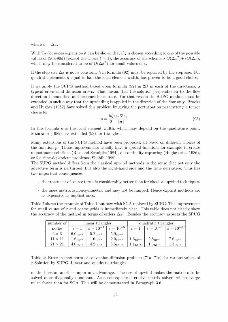
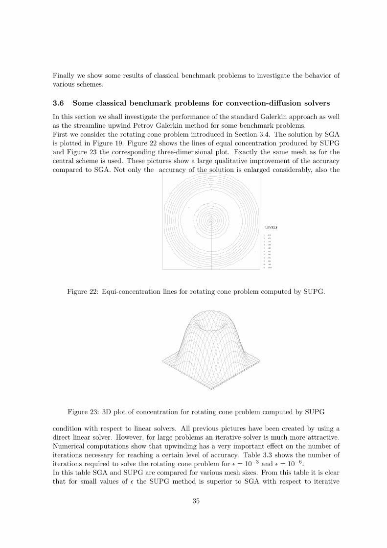
In this section we shall investigate the performance of the standard Galerkin approach as wellas the streamline upwind Petrov Galerkin method for some benchmark problems.First we consider the rotating cone problem introduced in Section 3.4. The solution by SGAis plotted in Figure 19. Figure 22 shows the lines of equal concentration produced by SUPGand Figure 23 the corresponding three-dimensional plot. Exactly the same mesh as for thecentral scheme is used. These pictures show a large qualitative improvement of the accuracycompared to SGA. Not only the accuracy of the solution is enlarged considerably, also the
1
2
2
3
3
4
4
5
5
6
6
7
7
8
8
9
9
10
10
11
LEVELS
1 -.029
2 .075
3 .179
4 .284
5 .388
6 .492
7 .597
8 .701
9 .806
10 .910
11 1.014
Figure 22: Equi-concentration lines for rotating cone problem computed by SUPG.
Figure 23: 3D plot of concentration for rotating cone problem computed by SUPG
condition with respect to linear solvers. All previous pictures have been created by using adirect linear solver. However, for large problems an iterative solver is much more attractive.Numerical computations show that upwinding has a very important effect on the number ofiterations necessary for reaching a certain level of accuracy. Table 3.3 shows the number ofiterations required to solve the rotating cone problem for ǫ = 10−3 and ǫ = 10−6.In this table SGA and SUPG are compared for various mesh sizes. From this table it is clearthat for small values of ǫ the SUPG method is superior to SGA with respect to iterative
35
solvers.
SGA SUPG
ǫ number of nodes accuracy 10−3 accuracy 10−6 accuracy 10−3 accuracy 10−6
10−3 21× 21 15 19 6 941× 41 17 21 6 981× 81 31 38 27 32
10−6 21× 21 - - 9 1241× 41 - - 13 1781× 81 - - 24 32
Table 3: Number of iterations by a preconditioned CGS solver for the solution of the rotatingcone problem of Section 3.4. SGA and SUPG. A - in the table means that no convergencewas possible.
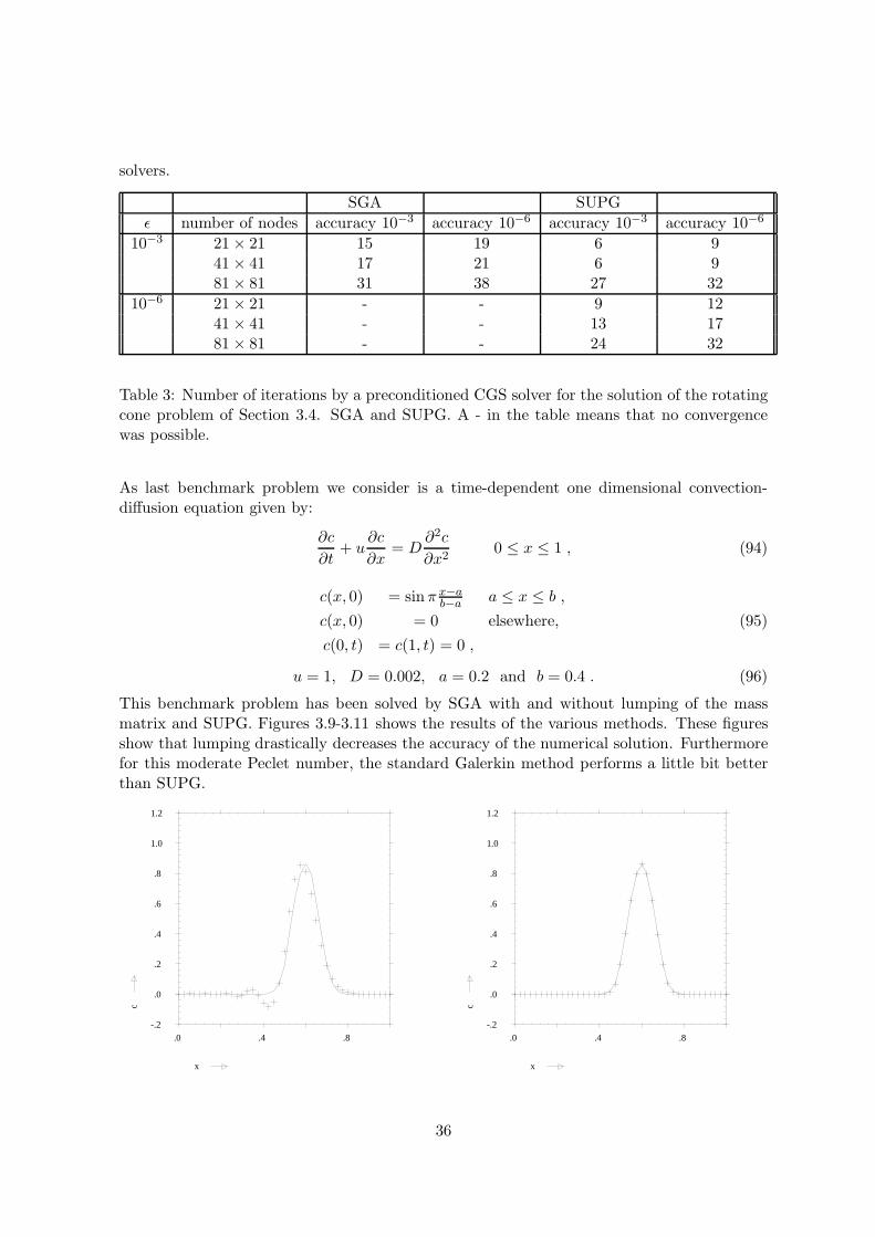
As last benchmark problem we consider is a time-dependent one dimensional convection-diffusion equation given by:
∂c
∂t+ u
∂c
∂x= D
∂2c
∂x20 ≤ x ≤ 1 , (94)
c(x, 0) = sinπ x−ab−a
a ≤ x ≤ b ,
c(x, 0) = 0 elsewhere, (95)
c(0, t) = c(1, t) = 0 ,
u = 1, D = 0.002, a = 0.2 and b = 0.4 . (96)
This benchmark problem has been solved by SGA with and without lumping of the massmatrix and SUPG. Figures 3.9-3.11 shows the results of the various methods. These figuresshow that lumping drastically decreases the accuracy of the numerical solution. Furthermorefor this moderate Peclet number, the standard Galerkin method performs a little bit betterthan SUPG.
.0 .4 .8
-.2
.0
.2
.4
.6
.8
1.0
1.2
x
c
.0 .4 .8
-.2
.0
.2
.4
.6
.8
1.0
1.2
x
c
36
Figure 3.9:SGA applied to (3.40)-(3.42)40 linear elements, lumped mass matrix– exact solution, + numerical solution
Figure 3.10:SGA applied to (3.40)-(3.42)40 linear elements, consistent mass matrix– exact solution, numerical solution
37

.0 .4 .8
-.2
.0
.2
.4
.6
.8
1.0
1.2
x
c
Figure 24: SUPG with stationary upwind parameter applied to (3.40)-(3.42), 40 linear ele-ments: – exact solution, + numerical solution
38
4 Discretization of the incompressible Navier-Stokes equations
by standard Galerkin
4.1 The basic equations of fluid dynamics
In this chapter we shall consider fluids with the following properties:
• The medium is incompressible,
• The medium has a Newtonian character,
• The medium properties are temperature independent and uniform,
• The flow is laminar.
For a three-dimensional flow field the basic equations of fluid flow under the above restrictions,can be written as:The Continuity equation
div u =∂u1∂x1
+∂u2∂x2
+∂u3∂x3
= 0 . (97)
The Navier-Stokes equations
ρ
(
∂u
∂t+ (u.∇)u
)
− div σ = ρf , (98)
in which u = (u1, u2, u3)T denotes the velocity vector, ρ the density of the fluid, f =
(f1, f2, f3) the body force per unit of mass, and σ the stress tensor.Component-wise (98) reads:
ρ
(
∂ui∂t
+ u1∂ui∂x1
+ u2∂ui∂x2
+ u3∂ui∂x3
)
−(
∂σi1∂x1
+∂σi2∂x2
+∂σi3∂x3
)
= ρ fi, (i = 1, 2, 3) .
(99)For an incompressible and isotropic medium the stress terms σ can be written as
σ = −p I + d = −p I + 2µ e , (100)
where p denotes the pressure,I the unit tensore the rate of strain tensor,d the deviatoric stress tensor andµ the viscosity of the fluid.
The components eij of the tensor e are defined by
eij =1
2
(
∂ui∂xj
+∂uj∂xi
)
, (101)
so
σij = −pδij + µ
(
∂ui∂xj
+∂uj∂xi
)
. (102)
39
If µ is constant it is possible to simplify the expression(98) by substitution of the incompress-ibility condition (97) to
ρ
(
∂u
∂t+ (u . ∇)u
)
− µ u+∇ p = ρf , (103)
however, we shall prefer expression (98) because boundary conditions will be implementedmore easily in (98) than in (103).
Equation (98) can be made dimensionless by the introduction of the Reynolds number Redefined by
Re =ρUL
µ, (104)
where U is some characteristic velocity and L a characteristic length. Substitution of (104)into (98), (100) gives
∂u
∂t+ (u . ∇)u− div σ = f (105a)
σ = −p I +2
Ree (105b)
provided ρ does not depend on the space coordinates.
4.2 Initial and boundary conditions
In order to solve the equations (97), (98), it is necessary to prescribe both initial and boundaryconditions. Since only first derivatives of time are present in (98), it is sufficient to prescribethe initial velocity field at t = 0. Of course this velocity field must satisfy the incompressibil-ity condition (97)
Since (98) is a system of second order differential equations in space, it is necessary to pre-scribe boundary conditions for each velocity component on the complete boundary of thedomain. However, at high Reynolds numbers the convective terms dominate the stress tensorand as a consequence the boundary conditions at outflow must be such that they restrict theflow as little as possible.The continuity equation and the pressure play a very special role in the incompressible Navier-Stokes equations. In fact there is a strong relation between both. It can be shown (Ladyshen-skaya, 1969), that for incompressible flows no explicit boundary conditions for the pressuremust be given. Usually boundary conditions for the pressure are implicitly given by prescrib-ing the normal stress.
The following types of boundary conditions are commonly used for the two-dimensional in-compressible Navier-Stokes equations (the extension to IR3 is straight forward):
1 u given (Dirichlet boundary condition), (106a)
2 un and σnt given, (106b)
3 ut and σnn given, (106c)
4 σnt and σnt given, (106d)
40
where un denotes the normal component of the velocity on the boundary and ut the tangentialcomponent. σnn (n·σ ·n) denotes the normal component of the stress tensor on the boundaryand σnt (n · σ · t) the tangential component.
Typical examples of these boundary conditions are:
• At fixed walls: no-slip condition u = o. This is an example of type (106b).
• At inflow the velocity profile given: u = g. This is also an example of type (106b).Typical inflow profiles are ut = 0, un parabolic or ut = 0 and un constant.
At outflow one may prescribe the velocity. However, for convection dominated flows, such aboundary condition may lead to wiggles due to inaccuracies of the boundary conditions. Lessrestrictive boundary conditions are for example ut = 0 and σnn = 0 or σnt = 0 and σnn = 0.The first one (ut = 0, σnn = 0) prescribes a parallel outflow with zero normal stress. From(102) it can be derived that
σnn = −p+ 2
Re
∂un∂n
, (107)
and σnt =1
Re
(
∂un∂t
+∂ut∂n
)
. (108)
As a consequence for high Reynolds numbers σnn is approximately equal to −p. So σnn = 0implies that implicitly p is set equal to zero.The boundary condition ut = 0, σnn = 0 is correct for channel flow. The boundary conditionσnt = 0, σnn = 0 is in general not correct. For a channel flow, in which case we have aparabolic velocity profile, ∂un
∂tis linear and hence σnt 6= 0. However, in practical situations we
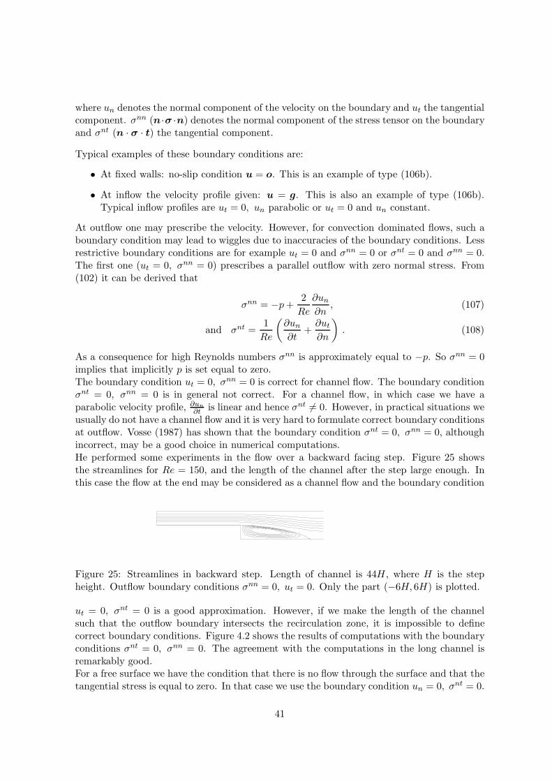
usually do not have a channel flow and it is very hard to formulate correct boundary conditionsat outflow. Vosse (1987) has shown that the boundary condition σnt = 0, σnn = 0, althoughincorrect, may be a good choice in numerical computations.He performed some experiments in the flow over a backward facing step. Figure 25 showsthe streamlines for Re = 150, and the length of the channel after the step large enough. Inthis case the flow at the end may be considered as a channel flow and the boundary condition
1 2 34 5
67
Figure 25: Streamlines in backward step. Length of channel is 44H, where H is the stepheight. Outflow boundary conditions σnn = 0, ut = 0. Only the part (−6H, 6H) is plotted.
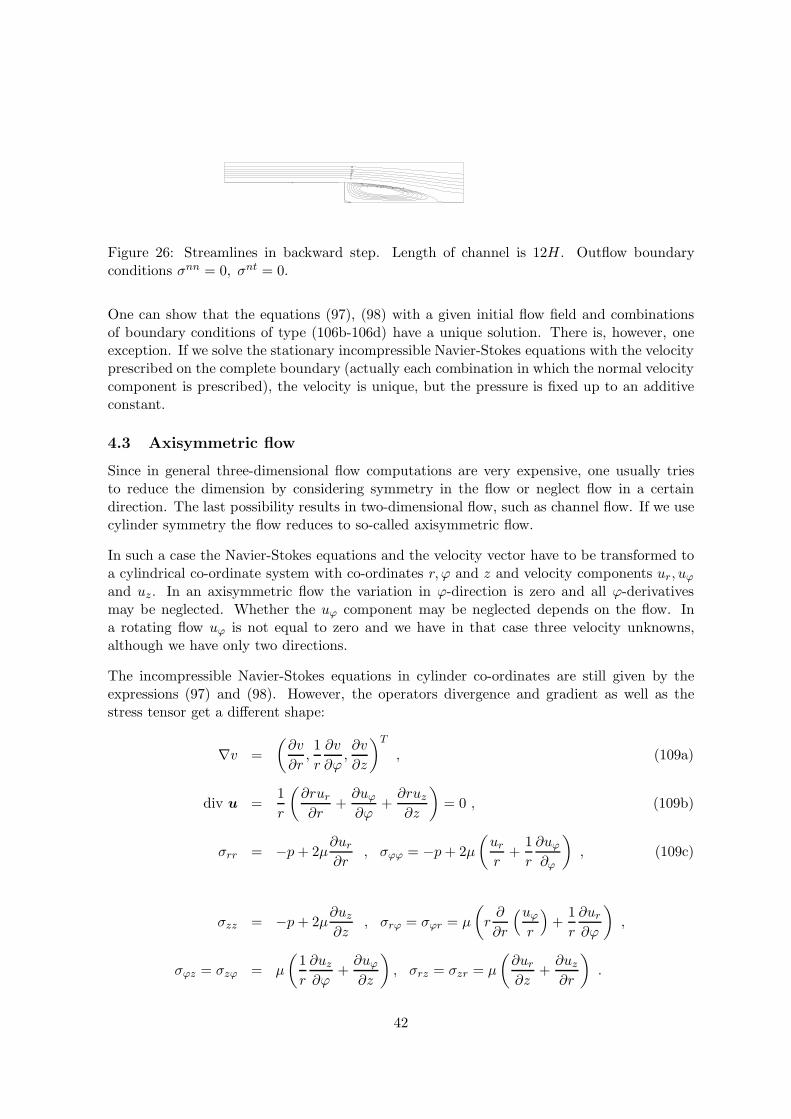
ut = 0, σnt = 0 is a good approximation. However, if we make the length of the channelsuch that the outflow boundary intersects the recirculation zone, it is impossible to definecorrect boundary conditions. Figure 4.2 shows the results of computations with the boundaryconditions σnt = 0, σnn = 0. The agreement with the computations in the long channel isremarkably good.For a free surface we have the condition that there is no flow through the surface and that thetangential stress is equal to zero. In that case we use the boundary condition un = 0, σnt = 0.
41
1 2 34 5
67
7
7
8910111213
Figure 26: Streamlines in backward step. Length of channel is 12H. Outflow boundaryconditions σnn = 0, σnt = 0.
One can show that the equations (97), (98) with a given initial flow field and combinationsof boundary conditions of type (106b-106d) have a unique solution. There is, however, oneexception. If we solve the stationary incompressible Navier-Stokes equations with the velocityprescribed on the complete boundary (actually each combination in which the normal velocitycomponent is prescribed), the velocity is unique, but the pressure is fixed up to an additiveconstant.
4.3 Axisymmetric flow
Since in general three-dimensional flow computations are very expensive, one usually triesto reduce the dimension by considering symmetry in the flow or neglect flow in a certaindirection. The last possibility results in two-dimensional flow, such as channel flow. If we usecylinder symmetry the flow reduces to so-called axisymmetric flow.
In such a case the Navier-Stokes equations and the velocity vector have to be transformed toa cylindrical co-ordinate system with co-ordinates r, ϕ and z and velocity components ur, uϕand uz. In an axisymmetric flow the variation in ϕ-direction is zero and all ϕ-derivativesmay be neglected. Whether the uϕ component may be neglected depends on the flow. Ina rotating flow uϕ is not equal to zero and we have in that case three velocity unknowns,although we have only two directions.
The incompressible Navier-Stokes equations in cylinder co-ordinates are still given by theexpressions (97) and (98). However, the operators divergence and gradient as well as thestress tensor get a different shape:
∇v =
(
∂v
∂r,1
r
∂v
∂ϕ,∂v
∂z
)T
, (109a)
div u =1
r
(
∂rur∂r
+∂uϕ∂ϕ
+∂ruz∂z
)
= 0 , (109b)
σrr = −p+ 2µ∂ur∂r
, σϕϕ = −p+ 2µ
(
urr
+1
r
∂uϕ∂ϕ
)
, (109c)
σzz = −p+ 2µ∂uz∂z
, σrϕ = σϕr = µ
(
r∂
∂r
(uϕr
)
+1
r
∂ur∂ϕ
)
,
σϕz = σzϕ = µ
(
1
r
∂uz∂ϕ
+∂uϕ∂z
)
, σrz = σzr = µ
(
∂ur∂z
+∂uz∂r
)
.
42

Note that in these expressions the term 1/r frequently occurs. As a consequence one has tobe careful in the numerical computations at r = 0. At the symmetry axis r = 0, we needextra boundary conditions, the so-called symmetry conditions. One immediately verifies thatthese symmetry conditions are given by:
ur = 0 ,∂uz∂r
= 0 , uϕ = 0 at r = 0 , (110)
or translated to stresses:
ur = 0 , uϕ = 0 and σnt = 0 at r = 0 . (111)
4.4 The weak formulation
In the next paragraph we shall derive the standard Galerkin equation for the incompressibleNavier-Stokes equations. First we shall derive the weak formulation. In order to consider thefour boundary conditions (106b- 106d), we shall assume that the boundary consists of fourparts each with one of the boundary conditions (106b-106d). Furthermore we shall restrictourselves in this chapter to stationary problems. The instationary case will be treated inChapter 7.
G
GG
3G
W
4 1
2
Figure 27: Artificial example with region Ω and boundaries Γ1,Γ2,Γ3 and Γ4.
Furthermore we restrict ourselves for the moment to the two-dimensional case. Figure 4.3shows an artificial example of a region Ω with four boundaries Γ1 to Γ4. On each of theseboundaries we have a different type of boundary condition. The formulation of our exampleis now: For x ∈ Ω solve u satisfying
div u = 0 , (112a)
−div σ + ρ(u ·∇ u) = ρf , (112b)
σij = −pδij + µ
(
∂ui∂xj
+∂uj∂xi
)
, (112c)
u = g1 for x ∈ Γ1, (112d)
un = g2, σnt = g3 , x ∈ Γ2 , (112e)
ut = g4, σnn = g5 , x ∈ Γ3 , (112f)
σnt = g6 σnn = g7 , x ∈ Γ4 . (112g)
43
In order to derive the weak formulation, equation (112a-112b) must be multiplied by testfunctions. First equation (112a) is multiplied by a test function q resulting in
∫
Ω
q div u dΩ = 0 (113)
The momentum equations (112b) consist of two equations, which may be each multiplied byseparate test functions v1 and v2. If we define v = (v1, v2)
T these equations can be combinedto:
∫
Ω
(−div σ + ρ(u · ∇ u)) · v dΩ =
∫
Ω
f · v dΩ . (114)
Choosing v2 respectively v1 equal to zero gives us the original weak formulation for each ofthe equations.
The first term in (114) may be further reduced by applying integration by parts (Gausstheorem) to
∫
Ω
(−div σ) · v dΩ =
∫
Ω
σ · ∇ v dΩ −∫
Γ
(vn σnn + vt σ
nt)dΓ, (115)
where Γ denotes the boundary of Ω, vn the component of v in the normal direction and vt inthe tangential direction. For a derivation of formula (115) we refer to Appendix A.
In order to apply the boundary conditions (112d-112g), the boundary integral over Γ is splitinto 4 parts Γ1, to Γ4.On Γ1 we have a prescribed velocity and hence the test function v is chosen equal to zero.On boundary Γ2 un is prescribed and so vn is chosen equal to zero, and on boundary Γ3 ut isprescribed and vt is set equal to zero.
If we furthermore substitute relation (100) into (115), the first term of (114) can be writ-ten as:
∫
Ω
−(div σ) · v dΩ =
∫
Ω
2µ e · ∇ v dΩ −∫
Ω
p div v dΩ
−∫
Γ2
g3 vt dΓ −∫
Γ3
g5 vn dΓ −∫
Γ4
g6 vt + g7 vn dΓ . (116)
Combinations of all these results leads to the weak formulation of the Navier-Stokes equations(112a-112g):Find u , p with
u = g1 at Γ1 , un = g2 at Γ2 , ut = g4 at Γ3,
44
such that∫
Ω
q div u dΩ = 0 , (117)
∫
Ω
2µe · ∇ v dΩ +
∫
Ω
ρ(u · ∇ u) · v dΩ −∫
Ω
p div v dΩ =
∫
Γ2
g3 vt dΓ +
∫
Γ3
g5 vn dΓ +
∫
Γ4
g6 vt + g7 vn dΓ +
∫
Ω
ρf · v dΩ , (118)
for all v such that v = o at Γ1, vn = 0 at Γ2 and vt = 0 at Γ3, and e given by (101).
We see that in the relations (117) and (118) no derivatives of p and q are necessary. Henceit is sufficient that p and q are integrable. With respect to u and v, first derivatives arerequired and hence not only u and v but also their first derivatives must be integrable. Asa consequence we do not need continuity of p and q in the Galerkin formulation, but thefunctions u and v must be continuous over the element boundaries.
The weak formulation (117-118) shows a strong relation between u and v, as well as betweenp and q. If we for example demand that both u and v are divergence free, then the firstequation (117) vanishes and the pressure disappears from (118). Indeed in all theoreticalinvestigations with respect to the weak form of the Navier-Stokes equations, p and q aretaken from the same space and u and v are taken from the same space. This observationmotivates the choice of the basis functions in the standard Galerkin method.
4.5 The standard Galerkin method
In the standard Galerkin method we define two types of basis functions, basis function Ψi(x)corresponding to the pressure and functions ϕi(x) corresponding to the velocity components.We may combine the velocity basis functions into vector form by
ϕi1(x) =
(
ϕi(x)0
)
, ϕi2(x) =
(
0ϕi(x)
)
. (119)
Now the approximation of u and p will be defined by
ph =m∑
j=1
pj Ψj(x) , (120)
uh =n∑
j=1
u1j ϕj1(x) + u2j ϕj2(x) =2n∑
j=1
uj ϕj(x) . (121)
In (121) uj is defined by uj = u1j , (j = 1(1)n), uj+n = u2j , (j = 1(1)n) and ϕj in the sameway. For simplicity the summation has been carried out over all degrees of freedom includingthe prescribed ones at the boundary. The test functions, however, must only be coupled tothe free degrees of freedom. Mark that the number of basis functions ϕi(x) and Ψi(x) donot have to be the same, nor that these basis functions must have the same shape. In fact,in most practical applications ϕi(x) and Ψi(x) are chosen differently.
45

In order to get the standard Galerkin formulation we substitute v = ϕi(x), q = Ψi(x) intothe weak formulation (117-118).In this way we get:
Find pn and un defined by (120),(121) such that
∫
Ω
Ψi div uh dΩ = 0 , i = 1(1)m , (122)
and∫
Ω
2µ (eh · ∇ ϕi)dΩ+
∫
Ω
ρ(uh · ∇ uh) · ϕi dΩ
−∫
Ω
ph div ϕi) dΩ =
∫
Γ2
g3(ϕi · t) dΓ +
∫
Γ3
g5(ϕi · n) dΓ
+
∫
Γ4
g6(ϕi · t) + g7(ϕi · n) dΓ +
∫
Ω
ρf · ϕi dΩ
(123)
where eh is given by (101); u replaced by uh
i in (123) must be taken for all free degrees of freedom ui.
Expression (123) may be easily evaluated as long as n or t on the boundaries Γ2, Γ3 and Γ4
are in the direction of the co-ordinate axis. If they are not in that direction it is necessaryto transform the unknowns on the boundary locally such that they are expanded into normaland tangential direction. The technique of local transformations is described in Zienkiewiczand Taylor (1989).
The finite element method may be used to construct the basis functions ϕi and Ψi, in thesame way as for the potential problem in Chapter 1. Once the basis functions are known, theintegrals (122) and (123) may be evaluated element-wise. Finally we arrive at a system ofm+2n−np non-linear equations with m+2n−np unknowns, where np denotes the numberof prescribed boundary values, and m and N are defined in (120), (121).
Formally the system of equations can be written as
SU +N (U)−LTP = F (124a)
LU = o (124b)
where U denotes the vector of unknowns u1i and u2i, P denotes the vector of unknownspi, SU denotes the discretization of the viscous terms, N(U ) the discretization of the non-linear convective terms, LU denotes the discretization of the divergence of u and −LTP thediscretization of the gradient of p. The right-hand side F contains all contributions of thesource term, the boundary integral as well as the contribution of the prescribed boundaryconditions.
The solution of the system of equations (124a-124b) introduces two difficulties. Firstly theequations are non-linear and as a consequence some iterative solution procedure is necessary.
46
Secondly equation (124b) does not contain the unknown pressure P . The last aspect intro-duces a number of extra complications which will be treated in Paragraph 4.7. The non-lineariterative procedure will be the subject of Paragraph 4.6.
4.6 Treatment of the non-linear terms
In order to solve the system of non-linear equations, an iterative procedure is necessary. Ingeneral such a procedure consists of the following steps:
make an initial estimation
while (not converged) do
linearize the non-linear equations based on the previous solutionsolve the resulting system of linear equations
Examples of such methods are Newton methods, quasi-Newton methods, and Picard typemethods.
In order to derive the iterative method one may proceed in two ways. Firstly one can applythe method to equations (124a-124b), which is the classical approach. An alternative is tolinearize the non-linear differential equations first and then to discretize the resulting linearequation. Sometimes both approaches are identical. The last approach is conceptually easierthan the first one and will therefore be applied in this paragraph. Since it is the only non-linear term in equation (112a-112g) we only consider the convective terms.
Suppose we have computed the solution uk at a preceding iteration level k. We write this so-lution as uk. First we shall derive the Newton linearization. To that end we define f(u, ∇ u)as
f(u, ∇ u) = u · ∇ u . (125)
Taylor-series expansion of (125) gives
fk+1(u, ∇ u) = fk(
uk, ∇ uk)
+(
uk+1 − uk)
· ∂fk
∂u
+∇(
uk+1 − uk)
· ∂fk
∂∇u+O
(
uk+1 − uk)2
.
(126)
Neglecting the quadratic terms and substitution of (125) gives
uk+1 · ∇ uk+1 ≈ uk · ∇ uk +(
uk+1 − uk)
· ∇ uk +∇(
uk+1 − uk)
· uk
= uk+1 · ∇ uk + uk · ∇ uk+1 − uk · ∇ uk .(127)
(127) forms the standard Newton linearization. Alternative linearization are constructed bythe so-called Picard iteration methods in which one or both terms in (125) are taken at theold level.Hence:
(u · ∇ u)k+1 ≃ uk+1 · ∇ uk , (128)
(u · ∇ u)k+1 ≃ uk · ∇ uk+1 , (129)
(u · ∇ u)k+1 ≃ uk · ∇ uk . (130)
47
Numerical experiments have shown that from these last three possibilities only (129) producesa good convergence. (127) shows that Newton is in fact a linear combination of (128)-(130).After linearization of the convective terms the standard Galerkin method may be applied,resulting in a system of linear equations.An important question with respect to these iterative methods is, how to find a good initialestimate. It is well known that Newton’s method converges fast (i.e. quadratically) as soonas the iteration is in the neighborhood of the final solution. However, if the distance betweeniteration and solution is too large, Newton may converge slowly or even diverge. The Picarditeration seems to have a larger convergence region, which means that this iteration does notneed the same accurate initial estimate, however, this method converges only linearly.
A possible strategy to converge to the final solution is the following:
- start with some initial guess,
- perform one step Picard iteration in order to approach the final solution, sometimesmore than one step,
- use Newton iteration in the next steps.
An initial guess may be for example the solution of the Stokes problem, which is formed bythe Navier-Stokes equations where the convective terms have been neglected. If the Reynoldsnumber is too high it is possible that the distance between the solution of Stokes and Navier-Stokes is too large. In that case the solution of Navier-Stokes with a smaller Reynolds numbermight be a good choice. A process in which the Reynolds number is increased gradually iscalled a continuation method.
In general one may expect that the iteration process no longer converges as soon as the flowbecomes instationary or turbulent.
4.7 Necessary conditions for the elements
In Paragraph 4.5 it has been derived that the standard Galerkin method results in a system ofnon-linear equations of the form (124a-124b). After linearization this system can be writtenas
SU +N (Uk)U −LTP = F ,LU = o ,
(131)
where Uk is the solution of the previous iteration.
In Section 4.5 it has already been pointed out that with respect to the velocity it is neces-sary that the approximation over the element-sides must be continuous, whereas the pressureapproximation may be discontinuous over the element boundaries. However, there is an-other problem. The continuity equation, discretized as LU = o, does contain only velocityunknowns. However, the number of rows in this equation is completely determined by thenumber of pressure unknowns. Suppose that there are more pressure unknowns than velocityunknowns. In that case equation (131) contains more rows than unknowns and we have eithera dependent or inconsistent system of equations. In both cases the matrix to be solved issingular. So we have to demand that the number of pressure unknowns never exceeds thenumber of velocity unknowns. Since we want to solve the Navier-Stokes equations by finite
48
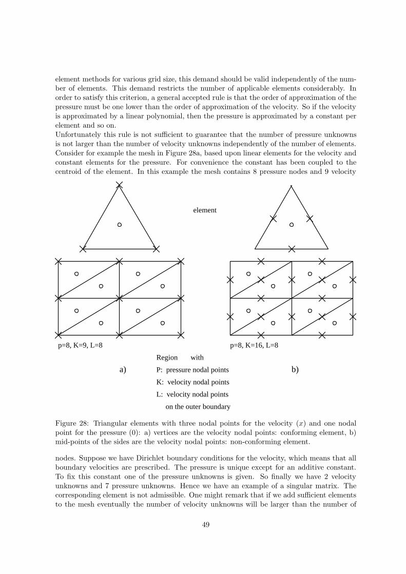
element methods for various grid size, this demand should be valid independently of the num-ber of elements. This demand restricts the number of applicable elements considerably. Inorder to satisfy this criterion, a general accepted rule is that the order of approximation of thepressure must be one lower than the order of approximation of the velocity. So if the velocityis approximated by a linear polynomial, then the pressure is approximated by a constant perelement and so on.Unfortunately this rule is not sufficient to guarantee that the number of pressure unknownsis not larger than the number of velocity unknowns independently of the number of elements.Consider for example the mesh in Figure 28a, based upon linear elements for the velocity andconstant elements for the pressure. For convenience the constant has been coupled to thecentroid of the element. In this example the mesh contains 8 pressure nodes and 9 velocity
b)
p=8, K=9, L=8 p=8, K=16, L=8
element
WRegion with
P: pressure nodal points
K: velocity nodal points
on the outer boundary
L: velocity nodal points
a)
Figure 28: Triangular elements with three nodal points for the velocity (x) and one nodalpoint for the pressure (0): a) vertices are the velocity nodal points: conforming element, b)mid-points of the sides are the velocity nodal points: non-conforming element.
nodes. Suppose we have Dirichlet boundary conditions for the velocity, which means that allboundary velocities are prescribed. The pressure is unique except for an additive constant.To fix this constant one of the pressure unknowns is given. So finally we have 2 velocityunknowns and 7 pressure unknowns. Hence we have an example of a singular matrix. Thecorresponding element is not admissible. One might remark that if we add sufficient elementsto the mesh eventually the number of velocity unknowns will be larger than the number of
49
pressure unknowns. However, practical computations have shown that in that case still thematrix remains singular.Figure 4.4b gives an example of an admissible element. The velocity unknowns are not posi-tioned in the vertices of the triangle but in the midside points. The velocity approximationis linear but not continuous over the element boundaries. Such an element is called non-conforming and introduces for that reason extra problems with the approximation. However,with respect to the continuity equation the element satisfies the demand that there must bemore velocity unknowns than pressure unknowns. A simple count shows that for the givenmesh, the number of velocity unknowns is equal to 16 and the number of pressure unknownsequal to 7 in the case of Dirichlet boundary conditions.The derivation of the admissibility condition given above is rather ad-hoc and does not ex-plain why an element is admissible. It just helps to identify non-admissible elements. In theliterature, see for example Cuvelier et al (1986), an exact admissibility condition is derived.This condition is known under the name Brezzi-Babuska condition (or BB condition). How-ever, the BB condition is rather abstract and in practice it is very difficult to verify whetherthe BB condition is satisfied or not. Fortin (1981) has given a simple method to check theBB condition on a number of elements.
The method is based on the following statement:
an element satisfies the BB condition, whenever, given a continuous differentiable vectorfield u, one can explicitly build a discrete vector field u such that:
∫
Ω
Ψi div u dΩ =
∫
Ω
Ψi div u dΩ for all basis functions Ψi . (132)
In Cuvelier et al (1986) it is demonstrated how (132) can be checked for a number of elements.
Fortin (1981) formulates the following engineering statement with respect to the admissibilityof elements.
Midside velocity points in two dimensions and centroid velocity points on surfaces inthree dimensions make it possible to control the amount of flow through a side (2D)and through a surface (3D) of an element, without altering the amount of flow throughother sides or surfaces. Hence such nodal points make it easier to satisfy the continuityequations.
In fact it is sufficient that the normal component of the velocity in these centroid points isavailable as unknowns.In the literature frequently elements are used, that do not satisfy the BB condition. Suchelements cannot be used with the standard Galerkin method, however the penalty functionmethod (see Chapter 5), permits the use of these elements.
4.8 Examples of admissible elements
In this section we shall treat some of the admissible elements for two-dimensional applica-tions. For a more thorough review as well as three-dimensional elements we refer to Cuvelieret al (1986) and Fortin (1981).
50
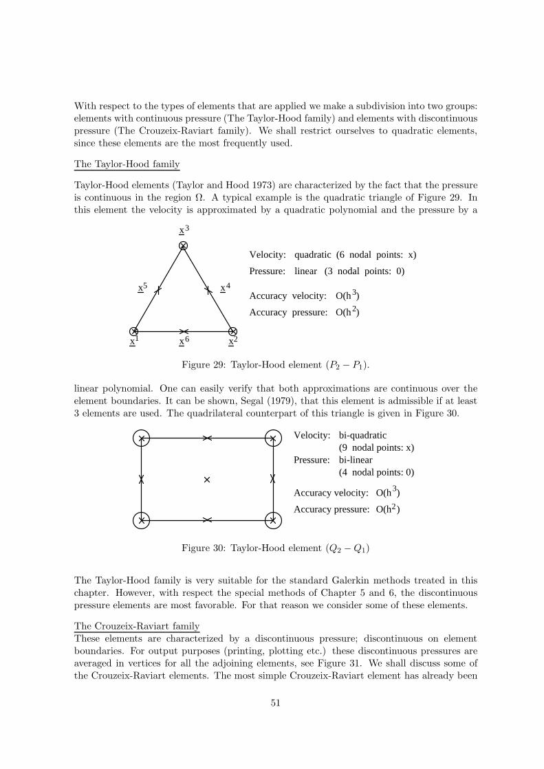
With respect to the types of elements that are applied we make a subdivision into two groups:elements with continuous pressure (The Taylor-Hood family) and elements with discontinuouspressure (The Crouzeix-Raviart family). We shall restrict ourselves to quadratic elements,since these elements are the most frequently used.
The Taylor-Hood family
Taylor-Hood elements (Taylor and Hood 1973) are characterized by the fact that the pressureis continuous in the region Ω. A typical example is the quadratic triangle of Figure 29. Inthis element the velocity is approximated by a quadratic polynomial and the pressure by a
2
Velocity:
x x x
xx
x3
5 4
1 6 2
quadratic (6 nodal points: x)
Pressure: linear (3 nodal points: 0)
Accuracy velocity:
Accuracy pressure:
O(h )3
O(h )
Figure 29: Taylor-Hood element (P2 − P1).
linear polynomial. One can easily verify that both approximations are continuous over theelement boundaries. It can be shown, Segal (1979), that this element is admissible if at least3 elements are used. The quadrilateral counterpart of this triangle is given in Figure 30.
2
(9 nodal points: x)Velocity:
(4 nodal points: 0)Pressure:
Accuracy velocity:
Accuracy pressure: O(h
O(h 3)
)
bi-linear
bi-quadratic
Figure 30: Taylor-Hood element (Q2 −Q1)
The Taylor-Hood family is very suitable for the standard Galerkin methods treated in thischapter. However, with respect the special methods of Chapter 5 and 6, the discontinuouspressure elements are most favorable. For that reason we consider some of these elements.
The Crouzeix-Raviart familyThese elements are characterized by a discontinuous pressure; discontinuous on elementboundaries. For output purposes (printing, plotting etc.) these discontinuous pressures areaveraged in vertices for all the adjoining elements, see Figure 31. We shall discuss some ofthe Crouzeix-Raviart elements. The most simple Crouzeix-Raviart element has already been
51
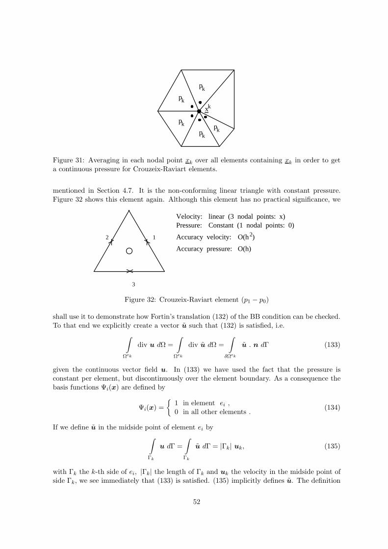
k
p
p
pp
p
x
kk
k
k
k
Figure 31: Averaging in each nodal point xk over all elements containing xk in order to geta continuous pressure for Crouzeix-Raviart elements.
mentioned in Section 4.7. It is the non-conforming linear triangle with constant pressure.Figure 32 shows this element again. Although this element has no practical significance, we
GG
G
O(h )
3
12
Velocity:Pressure:
Accuracy pressure:
Accuracy velocity:
Constant (1 nodal points: 0)linear (3 nodal points: x)
2
O(h)
Figure 32: Crouzeix-Raviart element (p1 − p0)
shall use it to demonstrate how Fortin’s translation (132) of the BB condition can be checked.To that end we explicitly create a vector u such that (132) is satisfied, i.e.
∫
Ωek
div u dΩ =
∫
Ωek
div u dΩ =
∫
δΩek
u . n dΓ (133)
given the continuous vector field u. In (133) we have used the fact that the pressure isconstant per element, but discontinuously over the element boundary. As a consequence thebasis functions Ψi(x) are defined by
Ψi(x) =
1 in element ei ,0 in all other elements .
(134)
If we define u in the midside point of element ei by
∫
Γk
u dΓ =
∫
Γk
u dΓ = |Γk| uk, (135)
with Γk the k-th side of ei, |Γk| the length of Γk and uk the velocity in the midside point ofside Γk, we see immediately that (133) is satisfied. (135) implicitly defines u. The definition
52
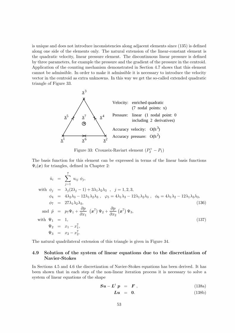
is unique and does not introduce inconsistencies along adjacent elements since (135) is definedalong one side of the elements only. The natural extension of the linear-constant element isthe quadratic velocity, linear pressure element. The discontinuous linear pressure is definedby three parameters, for example the pressure and the gradient of the pressure in the centroid.Application of the counting mechanism demonstrated in Section 4.7 shows that this elementcannot be admissible. In order to make it admissible it is necessary to introduce the velocityvector in the centroid as extra unknowns. In this way we get the so-called extended quadratictriangle of Figure 33.
Velocity:
2
x x x
xxx
x3
5 47
1 6 2
enriched quadratic
Pressure:
(7 nodal points: x)
linear (1 nodal point: 0including 2 derivatives)
Accuracy velocity: O(h )3
Accuracy pressure: O(h )
Figure 33: Crouzeix-Raviart element (P+2 − P1)
The basis function for this element can be expressed in terms of the linear basis functionsΨi(x) for triangles, defined in Chapter 2:
ui =7
∑
j=1
uij φj,
with φj = λj(2λj − 1) + 3λ1λ2λ3 , j = 1, 2, 3,
φ4 = 4λ2λ3 − 12λ1λ2λ3 , ϕ5 = 4λ1λ3 − 12λ1λ2λ3 , φ6 = 4λ1λ2 − 12λ1λ3λ3,
φ7 = 27λ1λ2λ3, (136)
and p = p7Ψ1 +∂p
∂x1
(
x7)
Ψ2 +∂p
∂x2
(
x7)
Ψ3,
with Ψ1 = 1, (137)
Ψ2 = x1 − x71,
Ψ3 = x2 − x72.
The natural quadrilateral extension of this triangle is given in Figure 34.
4.9 Solution of the system of linear equations due to the discretization ofNavier-Stokes
In Sections 4.5 and 4.6 the discretization of Navier-Stokes equations has been derived. It hasbeen shown that in each step of the non-linear iteration process it is necessary to solve asystem of linear equations of the shape
Su−Lt p = F , (138a)
Lu = 0. (138b)
53
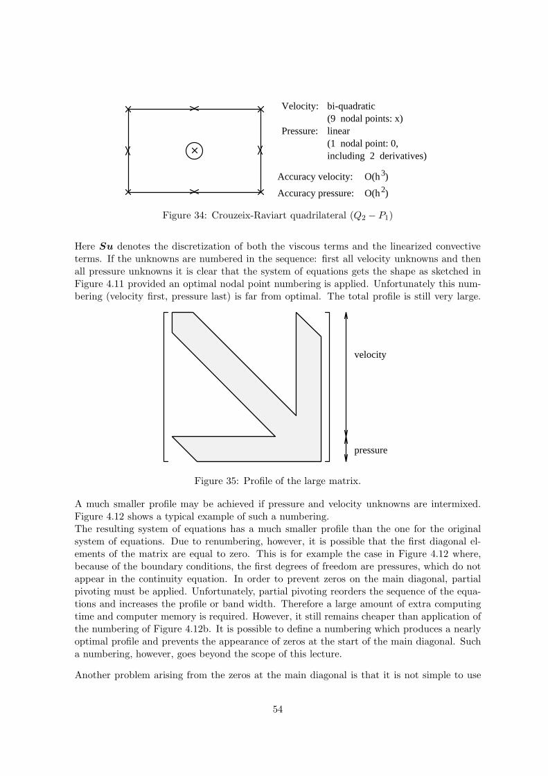
3
(9 nodal points: x)Velocity:
Pressure:
bi-quadratic
linear(1 nodal point: 0,including 2 derivatives)
Accuracy velocity:
Accuracy pressure: O(h )
O(h )2
Figure 34: Crouzeix-Raviart quadrilateral (Q2 − P1)
Here Su denotes the discretization of both the viscous terms and the linearized convectiveterms. If the unknowns are numbered in the sequence: first all velocity unknowns and thenall pressure unknowns it is clear that the system of equations gets the shape as sketched inFigure 4.11 provided an optimal nodal point numbering is applied. Unfortunately this num-bering (velocity first, pressure last) is far from optimal. The total profile is still very large.
velocity
pressure
Figure 35: Profile of the large matrix.
A much smaller profile may be achieved if pressure and velocity unknowns are intermixed.Figure 4.12 shows a typical example of such a numbering.The resulting system of equations has a much smaller profile than the one for the originalsystem of equations. Due to renumbering, however, it is possible that the first diagonal el-ements of the matrix are equal to zero. This is for example the case in Figure 4.12 where,because of the boundary conditions, the first degrees of freedom are pressures, which do notappear in the continuity equation. In order to prevent zeros on the main diagonal, partialpivoting must be applied. Unfortunately, partial pivoting reorders the sequence of the equa-tions and increases the profile or band width. Therefore a large amount of extra computingtime and computer memory is required. However, it still remains cheaper than application ofthe numbering of Figure 4.12b. It is possible to define a numbering which produces a nearlyoptimal profile and prevents the appearance of zeros at the start of the main diagonal. Sucha numbering, however, goes beyond the scope of this lecture.
Another problem arising from the zeros at the main diagonal is that it is not simple to use
54
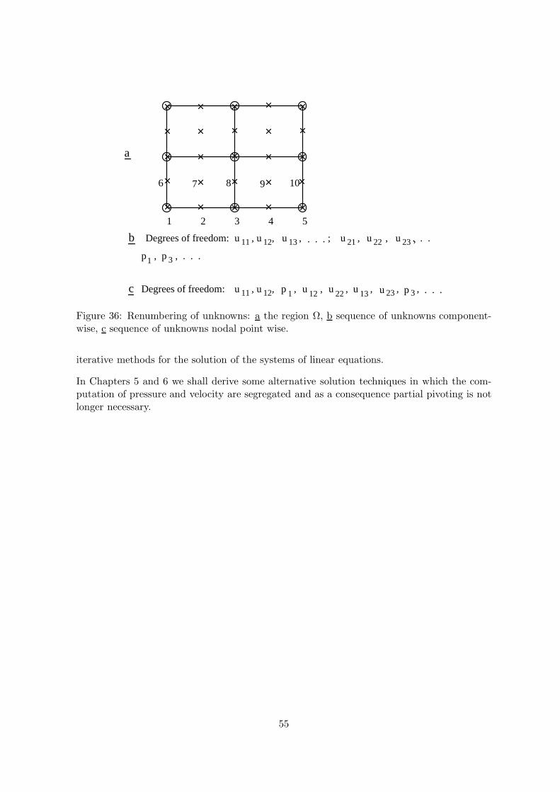
. . .
6 8 107 9
1 2 3 4 5
a
b . . .
p1 , p 3 , . . .
Degrees of freedom:
c Degrees of freedom: u , u ,1211 p 1 , u
u , u ,1211 u , . . . ; u 21 , u 22 , u 23 ,
12 ,
13
u 22 , u 13 , u 23 , p 3 ,
Figure 36: Renumbering of unknowns: a the region Ω, b sequence of unknowns component-wise, c sequence of unknowns nodal point wise.
iterative methods for the solution of the systems of linear equations.
In Chapters 5 and 6 we shall derive some alternative solution techniques in which the com-putation of pressure and velocity are segregated and as a consequence partial pivoting is notlonger necessary.
55
5 The penalty function method
5.1 Introduction
In Chapter 4 the discretization of the Navier-Stokes equations has been derived. It hasbeen shown that the direct solution of the resulting system of linear equations introducesextra complications due to the absence of the pressure in the incompressibility constraint.In this chapter we shall discuss a method which tries to solve this problem by segregatingcomputation of velocity and pressure. For the sake of simplicity we shall restrict ourselves tothe stationary Stokes equations, the extension to the instationary and to the non-linear caseis straightforward.
Consider the stationary linear Stokes equation in dimensionless form:
− 1
Re∆u+∇p = f , (139a)
div u = 0 . (139b)
(139a) follows from (105a) by neglecting the time-derivative and the convective terms, sub-stitution of (105b) and the incompressibility condition in (105a-105b). For the sake of theargument we restrict ourselves to homogeneous Dirichlet boundary conditions:
u = 0 x ∈ ∂Ω (140)
The pressure p is unique up to an additive constant. The idea of the penalty method is toperturb the continuity equation (139b) by a small term containing the pressure. An obviouschoice is
εp + div u = o , (141)
however, in the literature several other possibilities have been proposed.
The pressure p can be eliminated from (141) and substituted into (139a) resulting in anequation for the velocity:
p = −1
εdiv u , (142)
− 1
Re∆u− 1
ε∇(div u) = f . (143)
So one can first solve the velocity from (143) and afterwards compute the pressure directlyfrom (142). Such an approach will be called segregated approach.
The perturbation (141) makes only sense if the solution of (142), (143) approaches the solutionof (139a-139b) for ε approaching zero. It is a simple mathematical exercise to show that thisis indeed the case. See for example Cuvelier et al (1986) for the details.
The discretization of the penalty function method may be applied in two ways. One mayfirst discretize the Stokes equations and then apply the penalty function method, or one maydiscretize the formulation (142), (143). Both approaches will be treated separately in theSections 5.2 and 5.3.
56
Remark: the origin of the penalty method is motivated by the theory of optimization withconstraints. One can show (see Chapter 6) that (139a-139b) is equivalent to the con-strained minimization problem:
∫
Ω
1
2
1
Re|∇u|2 − u · f dΩ , (144)
for all functions u satisfying divu = 0.
5.2 The discrete penalty functions approach
In the discrete penalty function method, the (Navier-)stokes equations are discretized beforeapplying the penalty function method. So we start with the formulation (138a-138b):
Su− LTp = F , (145a)
Lu = 0 . (145b)
The continuity equation is perturbed by a term εMpp, where Mp is the so-called pressuremass matrix, defined by
Mp(i, j) =
∫
Ω
ψiψjdΩ , (146)
HenceεM pp+Lu = 0 , (147)
or
p = −1
εM−1
p Lu . (148)
Substitution of (148) in (145a) gives
(S +1
εLTM−1
p L)u = F . (149)
So u is computed from (149) and afterwards p is computed from (148). In exactly thesame way as for the continuous equation, it can be shown that the solution of (148), (149)approaches the solution of (145a-145b).
If we want to solve (148), (149), it is necessary that the matrix M−1p can be computed
easily. This is for example the case if Mp is a lumped mass matrix. In the discontinuouspressure elements, Mp is in a block diagonal matrix, i.e. a diagonal matrix consisting ofsmall matrices as diagonal elements. One can easily verify that these small matrices havethe size of the number of pressure unknowns per element, since Mp(i, j) = 0 if ψi and ψj
correspond to different elements. So for the Taylor-Hood family the matrix Mp is lumped,in the Crouzeix-Raviart family inversion of M p is quite simple.
Another practical aspect is that the building of the matrix LTM−1p L must be easy. Moreover,
it would be very nice if this matrix could be build per element by element matrices. In thatcase the structures of S and LTM−1
p L are identical and the solution of (149) is as simple asthe solution of Su = F . One can immediately verify that for the Taylor-Hood elements thisis not the case. Consider for example the simple triangular mesh in Figure 37. For simplicity
57
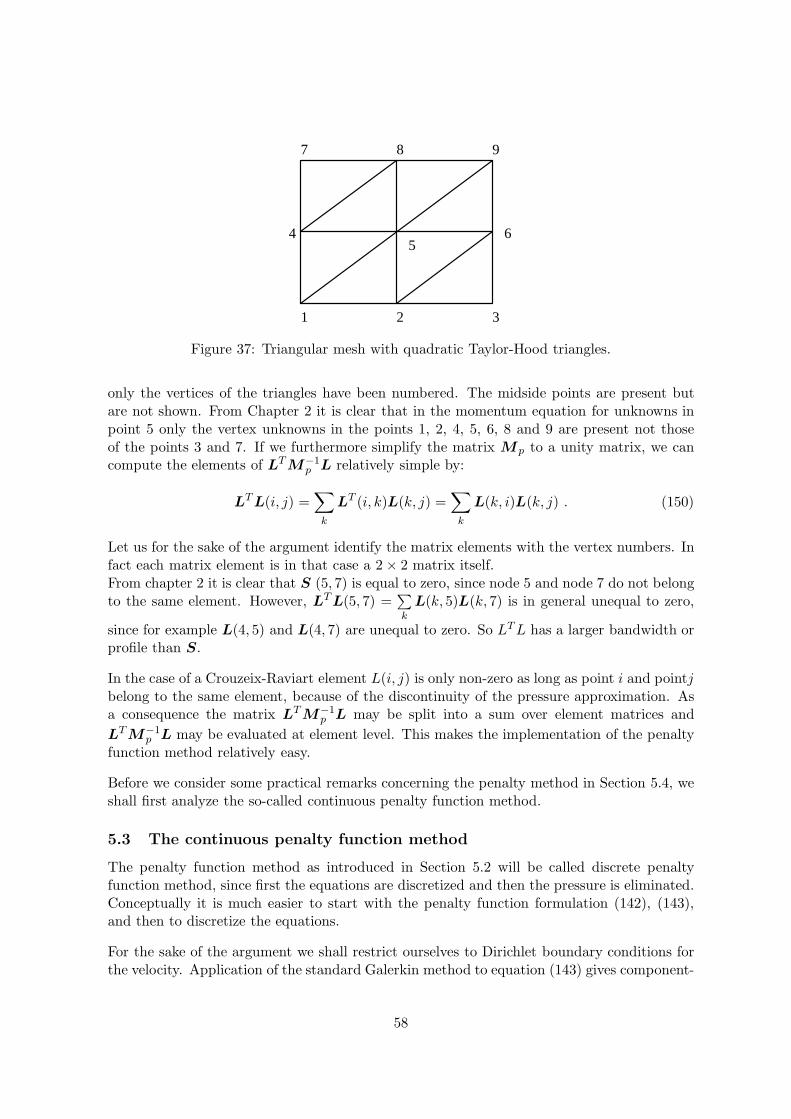
1 2
9
3
45
6
7 8
Figure 37: Triangular mesh with quadratic Taylor-Hood triangles.
only the vertices of the triangles have been numbered. The midside points are present butare not shown. From Chapter 2 it is clear that in the momentum equation for unknowns inpoint 5 only the vertex unknowns in the points 1, 2, 4, 5, 6, 8 and 9 are present not thoseof the points 3 and 7. If we furthermore simplify the matrix Mp to a unity matrix, we cancompute the elements of LTM−1
p L relatively simple by:
LTL(i, j) =∑
k
LT (i, k)L(k, j) =∑
k
L(k, i)L(k, j) . (150)
Let us for the sake of the argument identify the matrix elements with the vertex numbers. Infact each matrix element is in that case a 2× 2 matrix itself.From chapter 2 it is clear that S (5, 7) is equal to zero, since node 5 and node 7 do not belongto the same element. However, LTL(5, 7) =
∑
k
L(k, 5)L(k, 7) is in general unequal to zero,
since for example L(4, 5) and L(4, 7) are unequal to zero. So LTL has a larger bandwidth orprofile than S.
In the case of a Crouzeix-Raviart element L(i, j) is only non-zero as long as point i and pointjbelong to the same element, because of the discontinuity of the pressure approximation. Asa consequence the matrix LTM−1
p L may be split into a sum over element matrices and
LTM−1p L may be evaluated at element level. This makes the implementation of the penalty
function method relatively easy.
Before we consider some practical remarks concerning the penalty method in Section 5.4, weshall first analyze the so-called continuous penalty function method.
5.3 The continuous penalty function method
The penalty function method as introduced in Section 5.2 will be called discrete penaltyfunction method, since first the equations are discretized and then the pressure is eliminated.Conceptually it is much easier to start with the penalty function formulation (142), (143),and then to discretize the equations.
For the sake of the argument we shall restrict ourselves to Dirichlet boundary conditions forthe velocity. Application of the standard Galerkin method to equation (143) gives component-
58
wise:∫
Ω
1
Re∇(uh)k ·∇ϕi +
1
εdiv uh
∂ϕi
∂xkdΩ =
∫
Ω
fkϕidΩ , (151)
i = 1, 2, ..., n; k = 1, 2, 3,
where (uh)k denotes the k-th component of uh and fk the k-th component of f .In matrix vector notation (151) can be written as
Su+1
εAu = F . (152)
A clear advantage of the formulation (152) is that it is no longer necessary to computethe matrix LTM−1
p L and as a consequence Taylor-Hood elements are as simple as Crouzeix-Raviart elements. However, a closer examination of (151) shows that (152) has a disadvantagewhich is not present in (149).
If in (149) we let ε approach zero, it is immediately clear that
LTM−1p Lu → 0 , (153)
and it is easy to show that alsoLu → 0 . (154)
From (152) it follows that ε→ 0 implies
Au → 0 , (155)
or∫
Ω
div undiv ϕidΩ = 0 , (156)
for all basis functions ϕi.(156) is equivalent to (122), where div ϕiplays the role of the basis function ψi.Now consider the quadratic Taylor-Hood element. In equation (156) div ϕi is a linear dis-continuous polynomial. So relation (156) is comparable to the discretization of the continuityequation for a quadratic Crouzeix-Raviart element with linear pressure. From Section 4.8,however, we know that such an element is not admissible.
Although the penalty function formulation does not give rise to singular systems of equations,still one can expect some troubles with elements which in the limit approach non-admissibleelements. Indeed, computations with this approach, show that the velocity behaves rathergood, but that the pressure produce unrealistic wiggles (Sani et al 1981). These wiggles aregenerally known as spurious modes or checkerboard modes for the pressure.
In the literature non-admissible elements are frequently used. To suppress the wiggles oneeither uses some filtering (smoothing) of the computed pressure, or the penalty matrix iscomputed with a so-called reduced integration technique (Malhus et al 1978). The filteringtechnique may produce nice results, however, this technique is not so easy at non-rectangulargrids. With the reduced integration technique, actually the term
∫
Ω
div uhdiv ϕidΩ is approx-
imated by an inaccurate quadrature rule. This is comparable to approximating div ϕi by
59
a lower degree polynomial. As a consequence the actual pressure approximation is reduced,leading to an admissible but less accurate element.
From the discussion given above it is clear that the discrete penalty function approach is su-perior above the continuous penalty method. In the remainder of this lecture we shall restrictourselves to this discrete form.
5.4 Practical aspects of the penalty function method
In the previous sections the continuous and discrete penalty function method have beenderived. It has been shown that the discrete penalty function method, applied to admissibleelements is the most recommendable. What remains is the choice of the parameter ε. It isclear that εmust be so small that the computed velocity and pressure approximates the actualsolution accurately. However, there is one draw back with respect to the penalty functionformulation. In fact we add the matrix 1
εLTM−1
p L to the matrix S in (149). The matrix S
corresponds to the discretization of a vector Laplacian equation (in the case of Stokes flow)or a convection-diffusion type vector equation (Navier-Stokes flow). It is well known that thismatrix is good conditioned and has nice properties for many kinds of solvers.
The matrix L is a m × 2n matrix, where in general m ≪ n. The maximal rank of L ism or m − 1, depending on the type of boundary conditions. As a consequence the rank ofthe 2n × 2n matrix LTL can also not exceed m or m − 1. The same is true for the matrixLTM−1
p L. As a consequence the penalty matrix is a singular matrix with a large numberof dependent rows. This penalty matrix is multiplied by a large number 1/ε and added to anon-singular matrix. It is very natural to assume that the resulting matrix has a conditionnumber which is proportional to 1/ε. Indeed practical computations show such a behavior.As a consequence ε may not be chosen too small since otherwise the condition of the resultingmatrix is so bad that an accurate numerical solution is not longer possible. As a rule of thethumb one may choose ε such that
‖εp‖ ≈ k‖u‖ , (157)
where k is some value between O(10−3) and O(10−9). This statement is based on a 64 bitsaccuracy for the computations, i.e. double precision arithmetic on a 32 - bits computer.Especially for very viscous flow, which for example appear in non-newtonian fluids, a goodchoice for ε may be hard to find.
The fact that we have to choose ε carefully is a clear disadvantage. The relative large condi-tion number has also another disadvantage. It is nearly impossible to solve the matrix withstandard iterative techniques. Only if we enlarge the value of ε and use some outer iterativeprocedure, it is possible to use penalty function type methods in combination with iterativelinear solvers. A well known outer iterative procedure is the so-called Uzawa scheme (Cuvelieret al 1986), which is however, beyond the scope of this lecture.
Despite the clear disadvantages of the penalty function method, still this method is verypopular. The reason is that it is a rather simple and fast method, provided the number ofunknowns are not too large. The segregation of pressure and velocity gives a large reductionin computing time compared to the direct solution of the original equations. Only for largethree-dimensional problems, direct linear solvers become so expensive that it is practically
60
nearly impossible to apply this method.
In the next chapter we shall derive an alternative segregated method to solve the incompress-ible Navier-Stokes equations, the so-called solenoidal approach.
61
6 Divergence-free elements
6.1 Introduction
In Chapter 4 we have treated the standard Galerkin approach. It has been shown that thismethod may be applied, provided an admissible element is used. A clear disadvantage of theGalerkin method is the unavailability of the pressure in the continuity equation, and as aconsequence the presence of zeros on the main diagonal of the equations (138a-138b). As aconsequence the solution of the equations introduces extra difficulties. In the penalty functionmethod we have solved this problem by segregating pressure and velocity, thus reducing thenumber of unknowns as well as avoiding the zeros at the main diagonal. The only problemwith this method is that it is sometimes difficult to get a good of choice of the small parameterε and the bad condition of the remaining system of equations. Especially for very viscous(non-newtonian fluids) this may be a problem. In this chapter we shall derive an alternativesegregated approach in which it is not necessary to choose some parameter, and which doesnot lead to ill conditioned systems of equations.To that end we consider the weak formulation (117-118). If for the sake of simplicity we neglectboth the convective terms and all boundary integrals, substitute the continuity equation inthe stress tensor and use the dimensionless form, (117-118) can be written as:
∫
Ω
q div udΩ = 0 , (158a)
∫
Ω
1
Re∇u ·∇vdΩ−
∫
Ω
p div vdΩ =
∫
Ω
f · vdΩ . (158b)
Except with respect to the essential boundary conditions, u and v are chosen in the samespace. So if we restrict this space to all divergence-free vector fields, then it is immediatelyclear that (158a) is satisfied automatically and, moreover,
∫
Ω
p div vdΩ vanishes. In other
words an equation in the velocity alone remains. Unfortunately it is very hard to find functionswhich are completely divergence-free. However, formulation (158a-158b) shows that it is notnecessary to demand div u = 0, but that it is sufficient to weaken this statement to
∫
Ω
q div vdΩ = 0 for all q . (159)
If both our test functions and the solution u satisfy (159), (158a) is satisfied and (158b)reduced to
∫
Ω
1
Re∇u ·∇vdΩ =
∫
Ω
f · vdΩ, for all v , (160)
which is again an equation for the velocity alone.If we construct a basis ϕi in the space of approximately divergence-free vector fields satisfying(159), (160) can be written as:
uh =
n∑
j=1
ujϕj(x) , (161a)
62
n∑
j=1
uj
∫
Ω
1
Re∇ϕj ·∇ϕidΩ =
∫
Ω
f ·ϕidΩ , i = 1(1)n . (161b)
The extension to the non-linear Navier-Stokes equations, the general form of stress tensorand non-vanishing boundary integrals is trivial.
The system of equations (161b) is of double Laplacian type (in IR2), and may be solved quiteeasily. The only problem is of course, how to construct basis functions that are divergence-freein the sense of (159). In Section 6.2 we shall show the construction of such basis functionsfor one specific element.
6.2 The construction of divergence-free basis functions for 2D elements
In this section we shall construct divergence-free basis functions in the sense of (159) for two-dimensional elements. The extension to IR3 is quite complicated and introduces a numberof extra problems. We refer to Cuvelier et al (1986) for a derivation. The construction ofdivergence-free basis functions is relatively simple for elements of the Crouzeix-Raviart type,how to construct such functions for Taylor-Hood elements is not known at this moment. Forsimplicity we shall restrict ourselves to triangular elements; the extension to quadrilateralsis straightforward. In fact we shall derive these basis functions for the extended quadratictriangle of Figure 33, with the basis functions given in (136). But in order to get some insightin the problems associated with this derivation we shall first consider the non-conforminglinear triangle with constant pressure given in Figure 32.
In general (159) can be written as∫
Ω
Ψi div uhdΩ = 0 for all pressure basis functions Ψi . (162)
In other words we have to construct basis functions ϕi such that∫
Ω
Ψj div ϕidΩ = 0 , for all Ψj . (163)
One may expect that the basis functions ϕi(x) satisfying (163), have vector components,which are both nonzero, so these will be linear combinations of the classical basis functionsdefined by (119).In order to find these linear combinations we recall that for the non-conforming element, (163)reduces to
∫
Ωej
div ϕidΩ = 0 , (164)
for all elements ej , since Ψj is one in element ej and zero outside the element.Application of the Gauss-divergence theorem to (164) gives
∫
Γej
ϕi · ndΓ = 0 , (165)
where Γej is the boundary of the triangle ej. In each triangle we have 6 unknown velocitiescorresponding to the three midside points. In all previous examples (compare with 121) these
63

velocity components were in fact the Cartesian components. However, for our purposes it isbetter to decompose the velocity in a tangential and a normal component along the boundaryof the triangle. See Figure 38 for a definition. In this element the velocity u is approximatedby
t
x x x
xx
x
x
x
x3
45
1 6 2
3
5
1
G
G GG 2
3
12
n
Figure 38: Element e, with boundary Γ2 separately plotted. Normal and tangential unityvectors on Γ2 are indicated.
uh =∑
k=2,4,6
u1kϕk1(x) + u2kϕk2(x) , (166)
which can be written as
uh =∑
k=2,4,6
unkϕkn(x) + utkϕkt(x) , (167)
where unk respectively utk denote the normal and tangential component of u in node k.ϕkn(x) and ϕkt(x) are defined by
ϕkn(x) = ϕk(x)nk , (168a)
ϕkt(x) = ϕk(x)tk . (168b)
Here ϕk(x) denotes the scalar basis function corresponding to point k and nk and tk thenormal respectively tangential vector corresponding to the edge on which node k is positioned.
The basis functions ϕkt(x) satisfy (165) exactly, since ϕk(x) = 1 on the edge containingnode k and linear from -1 to 1 at the other sides. On the edge containing node k we havenk · tk = 0, on the other edges n is constant and the integral over ϕk(x) vanishes becauseof the linearity. So one set of divergence-free basis functions is formed by the set of basisfunctions corresponding to the tangential components.
The other set of basis functions must be constructed such that (165) is satisfied. Now∫
Γk
uh · ndΓ (169)
defines the amount of flow through side Γk. For an incompressible flow one can define astream function Ψ by
u = (∂Ψ
∂y,−∂Ψ
∂x) . (170)
64
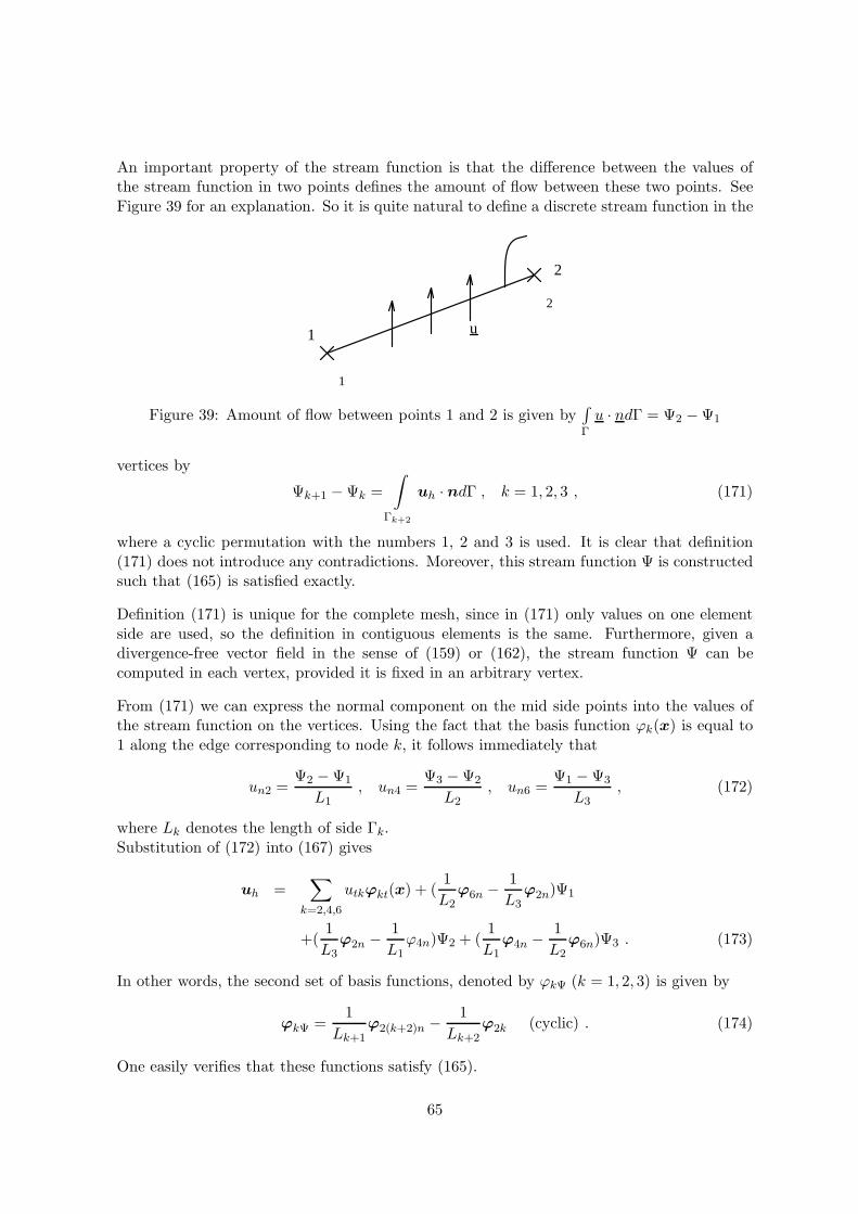
An important property of the stream function is that the difference between the values ofthe stream function in two points defines the amount of flow between these two points. SeeFigure 39 for an explanation. So it is quite natural to define a discrete stream function in the
2
1
2
u
G
Y
Y
1
Figure 39: Amount of flow between points 1 and 2 is given by∫
Γ
u · ndΓ = Ψ2 −Ψ1
vertices by
Ψk+1 −Ψk =
∫
Γk+2
uh · ndΓ , k = 1, 2, 3 , (171)
where a cyclic permutation with the numbers 1, 2 and 3 is used. It is clear that definition(171) does not introduce any contradictions. Moreover, this stream function Ψ is constructedsuch that (165) is satisfied exactly.
Definition (171) is unique for the complete mesh, since in (171) only values on one elementside are used, so the definition in contiguous elements is the same. Furthermore, given adivergence-free vector field in the sense of (159) or (162), the stream function Ψ can becomputed in each vertex, provided it is fixed in an arbitrary vertex.
From (171) we can express the normal component on the mid side points into the values ofthe stream function on the vertices. Using the fact that the basis function ϕk(x) is equal to1 along the edge corresponding to node k, it follows immediately that
un2 =Ψ2 −Ψ1
L1, un4 =
Ψ3 −Ψ2
L2, un6 =
Ψ1 −Ψ3
L3, (172)
where Lk denotes the length of side Γk.Substitution of (172) into (167) gives
uh =∑
k=2,4,6
utkϕkt(x) + (1
L2ϕ6n − 1
L3ϕ2n)Ψ1
+(1
L3ϕ2n − 1
L1ϕ4n)Ψ2 + (
1
L1ϕ4n − 1
L2ϕ6n)Ψ3 . (173)
In other words, the second set of basis functions, denoted by ϕkΨ (k = 1, 2, 3) is given by
ϕkΨ =1
Lk+1ϕ2(k+2)n − 1
Lk+2ϕ2k (cyclic) . (174)
One easily verifies that these functions satisfy (165).
65
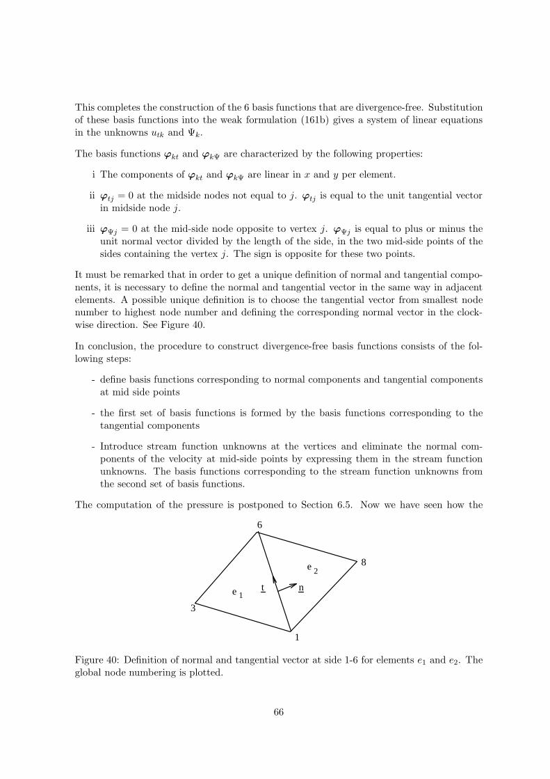
This completes the construction of the 6 basis functions that are divergence-free. Substitutionof these basis functions into the weak formulation (161b) gives a system of linear equationsin the unknowns utk and Ψk.
The basis functions ϕkt and ϕkΨ are characterized by the following properties:
i The components of ϕkt and ϕkΨ are linear in x and y per element.
ii ϕtj = 0 at the midside nodes not equal to j. ϕtj is equal to the unit tangential vectorin midside node j.
iii ϕΨj = 0 at the mid-side node opposite to vertex j. ϕΨj is equal to plus or minus theunit normal vector divided by the length of the side, in the two mid-side points of thesides containing the vertex j. The sign is opposite for these two points.
It must be remarked that in order to get a unique definition of normal and tangential compo-nents, it is necessary to define the normal and tangential vector in the same way in adjacentelements. A possible unique definition is to choose the tangential vector from smallest nodenumber to highest node number and defining the corresponding normal vector in the clock-wise direction. See Figure 40.
In conclusion, the procedure to construct divergence-free basis functions consists of the fol-lowing steps:
- define basis functions corresponding to normal components and tangential componentsat mid side points
- the first set of basis functions is formed by the basis functions corresponding to thetangential components
- Introduce stream function unknowns at the vertices and eliminate the normal com-ponents of the velocity at mid-side points by expressing them in the stream functionunknowns. The basis functions corresponding to the stream function unknowns fromthe second set of basis functions.
The computation of the pressure is postponed to Section 6.5. Now we have seen how the
3
2
1
8
6
t n
e
e 1
Figure 40: Definition of normal and tangential vector at side 1-6 for elements e1 and e2. Theglobal node numbering is plotted.
66
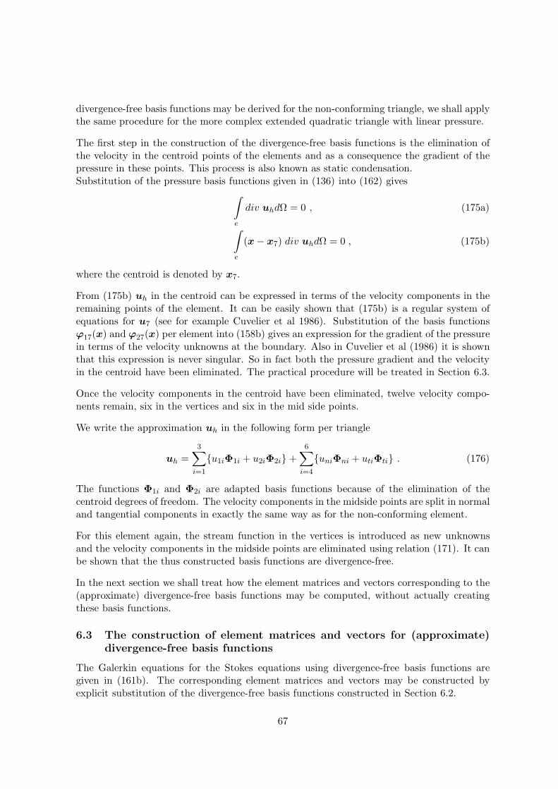
divergence-free basis functions may be derived for the non-conforming triangle, we shall applythe same procedure for the more complex extended quadratic triangle with linear pressure.
The first step in the construction of the divergence-free basis functions is the elimination ofthe velocity in the centroid points of the elements and as a consequence the gradient of thepressure in these points. This process is also known as static condensation.Substitution of the pressure basis functions given in (136) into (162) gives
∫
e
div uhdΩ = 0 , (175a)
∫
e
(x− x7) div uhdΩ = 0 , (175b)
where the centroid is denoted by x7.
From (175b) uh in the centroid can be expressed in terms of the velocity components in theremaining points of the element. It can be easily shown that (175b) is a regular system ofequations for u7 (see for example Cuvelier et al 1986). Substitution of the basis functionsϕ17(x) and ϕ27(x) per element into (158b) gives an expression for the gradient of the pressurein terms of the velocity unknowns at the boundary. Also in Cuvelier et al (1986) it is shownthat this expression is never singular. So in fact both the pressure gradient and the velocityin the centroid have been eliminated. The practical procedure will be treated in Section 6.3.
Once the velocity components in the centroid have been eliminated, twelve velocity compo-nents remain, six in the vertices and six in the mid side points.
We write the approximation uh in the following form per triangle
uh =
3∑
i=1
u1iΦ1i + u2iΦ2i+6
∑
i=4
uniΦni + utiΦti . (176)
The functions Φ1i and Φ2i are adapted basis functions because of the elimination of thecentroid degrees of freedom. The velocity components in the midside points are split in normaland tangential components in exactly the same way as for the non-conforming element.
For this element again, the stream function in the vertices is introduced as new unknownsand the velocity components in the midside points are eliminated using relation (171). It canbe shown that the thus constructed basis functions are divergence-free.
In the next section we shall treat how the element matrices and vectors corresponding to the(approximate) divergence-free basis functions may be computed, without actually creatingthese basis functions.
6.3 The construction of element matrices and vectors for (approximate)divergence-free basis functions
The Galerkin equations for the Stokes equations using divergence-free basis functions aregiven in (161b). The corresponding element matrices and vectors may be constructed byexplicit substitution of the divergence-free basis functions constructed in Section 6.2.
67
However, an alternative possibility is to start with the original set of equations (122), (123)using the classical basis functions and then to perform the elimination process. Let us demon-strate this process for the extended quadratic triangle. We shall execute the algorithm in twosteps. In the first step the centroid velocity components and the gradient of the pressure areeliminated. In the second step the normal components of the velocity at mid-side points areeliminated.
To perform step 1 we start with the system of linear equations (138a-138b):
Su−LTp = F , (177a)
Lu = 0 . (177b)
The velocity u will be split into a part corresponding to the centroid (uz) and the rest of thevelocities (u). In the same way the pressure p will be split into a part p∇ corresponding tothe gradient of the pressure in the centroid and a part p corresponding to the values of p inthe centroids. Hence we define
u =
[
u
uz
]
, p =
[
p
p∇
]
. (178)
If we split equations (177a-177b) according to (178) we get
S1u+ S2uz −LT2 p∇ = F , (179a)
L1u = L11u+L12uz = 0 , (179b)
L2u = L21u+L22uz = 0 . (179c)
The elimination of the velocity components in the centroid follows from (179c):
uz = −L−122 L21u , (180)
in other wordsu = Rzu , (181)
with
Rz =
[
I
R0
]
=
[
I
−L−122 L21
]
. (182)
From (182) we get
L2Rz = L21I +L22R0 = L21 −L22L−122 L21 = 0 , (183)
and hence alsoRT
z L2 = 0 . (184)
Substitution of (181) into (179a) gives:
S1u+ S2R0u−LT1 p−LT
2 p∇ = 0 . (185)
If we premultiply (185) by RTz and use (184) we get:
(RTz S1 +RT
z S2R0)u−RTz L
T1 p = RT
z F , (186)
68
and (179b) can be written asL1u = L1Rzu = 0 . (187)
In other words the result of the elimination process is
Su− LTp = F , (188a)
Lu = 0 , (188b)
with
S = RTz S1 +RT
z S2R0 , (189a)
L = L1Rz , (189b)
F = RTz F . (189c)
Due to the discontinuous character of the pressure, the matrices S and L and the right-handside vector F may be computed at element level.
The next step is the elimination of the normal components in the midside points in favor ofthe stream function at the vertices. This elimination process can be expressed by a matrixRd according to
u = Rdud , (190)
where ud is the vector of new unknowns.The transformation is such that the continuity equation is satisfied exactly in other words
LRd = 0 . (191)
Substitution of (191) in (188a-188b) and premultiplication by RTd gives
RTd SRdud = RT
d F . (192)
Again the matrix and vector can be constructed at elements level.
So we have shown that it is not necessary to construct the divergence-free basis functionsexplicitly. It is sufficient to construct the transformation matrices Rz and Rd per element andto compute the final element matrix and element right-hand side by matrix-matrix respectivelymatrix-vector multiplications.
We have constructed a new set of equations with new unknowns. The question that remainsis of course: is this new system of equations uniquely solvable? Furthermore, which type ofboundary conditions must be prescribed to the new unknowns. These questions will be thesubject of Section 6.4.
6.4 Boundary conditions with respect to the divergence-free elements
In the construction of the divergence-free elements treated in the preceding sections, it wasnecessary to introduce new unknowns. First of all the velocity has been decomposed intonormal and tangential part. With respect to the boundary conditions this does not introduceextra problems, since in general boundary conditions are formulated in tangential and normaldirection and not in Cartesian directions. Next the stream function has been introduced as
69
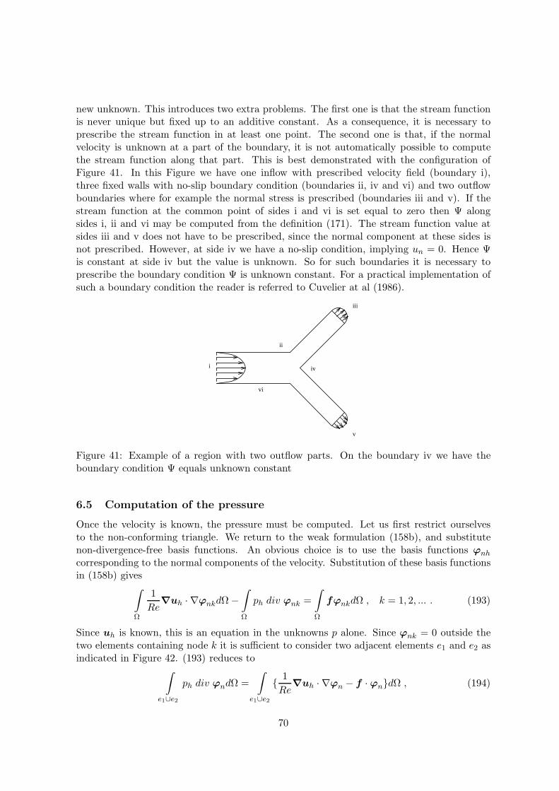
new unknown. This introduces two extra problems. The first one is that the stream functionis never unique but fixed up to an additive constant. As a consequence, it is necessary toprescribe the stream function in at least one point. The second one is that, if the normalvelocity is unknown at a part of the boundary, it is not automatically possible to computethe stream function along that part. This is best demonstrated with the configuration ofFigure 41. In this Figure we have one inflow with prescribed velocity field (boundary i),three fixed walls with no-slip boundary condition (boundaries ii, iv and vi) and two outflowboundaries where for example the normal stress is prescribed (boundaries iii and v). If thestream function at the common point of sides i and vi is set equal to zero then Ψ alongsides i, ii and vi may be computed from the definition (171). The stream function value atsides iii and v does not have to be prescribed, since the normal component at these sides isnot prescribed. However, at side iv we have a no-slip condition, implying un = 0. Hence Ψis constant at side iv but the value is unknown. So for such boundaries it is necessary toprescribe the boundary condition Ψ is unknown constant. For a practical implementation ofsuch a boundary condition the reader is referred to Cuvelier at al (1986).
v
ii
vi
i iv
iii
Figure 41: Example of a region with two outflow parts. On the boundary iv we have theboundary condition Ψ equals unknown constant
6.5 Computation of the pressure
Once the velocity is known, the pressure must be computed. Let us first restrict ourselvesto the non-conforming triangle. We return to the weak formulation (158b), and substitutenon-divergence-free basis functions. An obvious choice is to use the basis functions ϕnh
corresponding to the normal components of the velocity. Substitution of these basis functionsin (158b) gives
∫
Ω
1
Re∇uh · ∇ϕnkdΩ−
∫
Ω
ph div ϕnk =
∫
Ω
fϕnkdΩ , k = 1, 2, ... . (193)
Since uh is known, this is an equation in the unknowns p alone. Since ϕnk = 0 outside thetwo elements containing node k it is sufficient to consider two adjacent elements e1 and e2 asindicated in Figure 42. (193) reduces to
∫
e1∪e2
ph div ϕndΩ =
∫
e1∪e2
1
Re∇uh · ∇ϕn − f · ϕndΩ , (194)
70
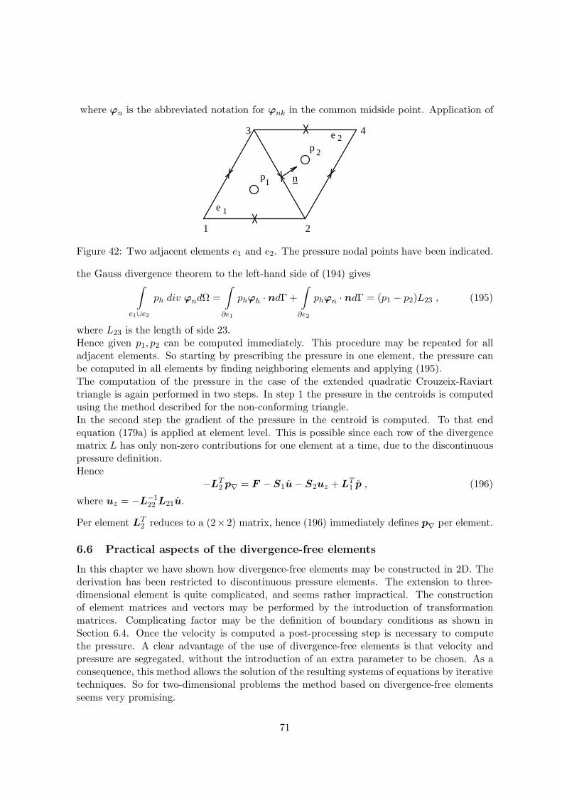
where ϕn is the abbreviated notation for ϕnk in the common midside point. Application of
2
1 2
e
e 43
n
1
2
p
p
1
Figure 42: Two adjacent elements e1 and e2. The pressure nodal points have been indicated.
the Gauss divergence theorem to the left-hand side of (194) gives∫
e1∪e2
ph div ϕndΩ =
∫
∂e1
phϕh · ndΓ +
∫
∂e2
phϕn · ndΓ = (p1 − p2)L23 , (195)
where L23 is the length of side 23.Hence given p1, p2 can be computed immediately. This procedure may be repeated for alladjacent elements. So starting by prescribing the pressure in one element, the pressure canbe computed in all elements by finding neighboring elements and applying (195).The computation of the pressure in the case of the extended quadratic Crouzeix-Raviarttriangle is again performed in two steps. In step 1 the pressure in the centroids is computedusing the method described for the non-conforming triangle.In the second step the gradient of the pressure in the centroid is computed. To that endequation (179a) is applied at element level. This is possible since each row of the divergencematrix L has only non-zero contributions for one element at a time, due to the discontinuouspressure definition.Hence
−LT2 p∇ = F − S1u− S2uz +LT
1 p , (196)
where uz = −L−122 L21u.
Per element LT2 reduces to a (2× 2) matrix, hence (196) immediately defines p∇ per element.
6.6 Practical aspects of the divergence-free elements
In this chapter we have shown how divergence-free elements may be constructed in 2D. Thederivation has been restricted to discontinuous pressure elements. The extension to three-dimensional element is quite complicated, and seems rather impractical. The constructionof element matrices and vectors may be performed by the introduction of transformationmatrices. Complicating factor may be the definition of boundary conditions as shown inSection 6.4. Once the velocity is computed a post-processing step is necessary to computethe pressure. A clear advantage of the use of divergence-free elements is that velocity andpressure are segregated, without the introduction of an extra parameter to be chosen. As aconsequence, this method allows the solution of the resulting systems of equations by iterativetechniques. So for two-dimensional problems the method based on divergence-free elementsseems very promising.
71
7 The instationary Navier-Stokes equations
7.1 Introduction
Until now we have restricted ourselves to stationary Navier-Stokes equations only. However,in some practical applications one is also interested in the time-dependent behavior of thesolution. Or, alternatively, sometimes it is hard to find the solution of a stationary problem,because the iteration process does not converge well enough. In that case, considering thestationary solution as limit of a time-dependent solution may help to get a convergent solution.For that reason we shall consider some methods to solve the time-dependent Navier-Stokesequations.
In first instance we shall use the method of lines as derived in Chapter 3. With respect to thediscretization of the continuity equation all three methods derived in the previous chaptersmay be applied. This well be the subject of Section 7.2.
In Section 7.3 an alternative approach will be treated, which is especially developed fortime-dependent incompressible flows. This method, the so-called pressure correction method,consists of two steps per time-step. In first instance the velocity is computed using the pressureat the old time-level and neglecting the continuity equation. In general, the computed velocityis not divergence-free. In the next step the velocity is projected onto the space of divergence-free vectors. This step also introduces a Laplacian type equation for the pressure.
7.2 Solution of the instationary Navier-Stokes equations by the method oflines
The instationary incompressible Navier-Stokes equations read (compare with 4.3):
ρ∂u
∂t+ ρu ·∇u− div σ = ρf , (197a)
div u = 0 . (197b)
In order to get a finite element discretization, the weak from of (197a) - (197b) is derived.To that end equation (197a) is multiplied by a time-independent test function v and (197b)by a test function q. If we neglect the boundary integrals and furthermore apply (100) in thesame way as for the stationary case, the weak form of (197a) may be written as
∫
Ω
ρ∂u
∂t· vdΩ+
∫
Ω
2µe ·∇vdΩ+
∫
Ω
ρ(u ·∇u)vdΩ−∫
Ω
pdiv vdΩ =
∫
Ω
f · vdΩ , (198a)
∫
Ω
q div udΩ = 0 . (198b)
We see that (198b) does not contain a time-derivative, and this will be an extra complicat-ing factor. If we approximate u and p in the same way as in (120), (121), however, withtime-dependent coefficients, and if we substitute the time-independent basis functions ϕi(x)
72
respectively Ψi(x), the Galerkin method reduces to the solution of a system of nonlinearordinary differential equations of the form
Mu+N (u)−LTp = F , (199a)
Lu = 0 , (199b)
whereN ,L,f ,u and p are defined as in (124a-124b) andM denotes the velocity mass matrix,which can be written as:
M =
(
M1 00 M1
)
, (200)
M 1(i, j) =
∫
Ω
ϕi(x)ϕj(x)dΩ .
The absence of a time-derivative in (199b) has as consequence that (199b) must be satisfiedin every stage of the time integration. An important consequence is that if the equations(199a-199b) are solved in a coupled way, explicit methods do not make sense. With respectto the time-integration, all the classical methods, such as for example the ones mentionedin Chapter 3 may be used. Very popular are the θ methods, especially θ = 1/2 and θ = 1,and the two-step Adams-Bashfort discretization. In this last formulation one usually usesan implicit formulation with respect to the viscous terms and an explicit formulation for theconvective terms. The reason for this splitting is that the matrix due to the convective termschanges in each time-step, whereas the other matrices remain constant in time.
Of course the solution of the coupled equations (199a-199b), introduces exactly the sameproblems as for the stationary case. As a consequence the same type of solution procedureswill be used. Hence it is quite usual to apply a segregated formulation in order to solve(199a-199b). Both the penalty function approach, as the method with divergence-free basisfunctions may be applied.
The penalty function approach, applied to (199a-199b) reads (compare with 150):
Mu+N (u) +1
εLTM−1
p Lu = F , (201a)
p = −1
εM−1
p Lu . (201b)
It is clear that the pressure has only to be computed, if at a certain moment the pressure isrequired. In the time-stepping algorithm it is sufficient to solve (201a).With respect to the non-linear terms, it is necessary to perform a kind of linearization. Ingeneral exactly the same type of linearization as for the stationary case are used. However,in contrast to the stationary case, no iteration per time-step is applied. In general, the non-linear terms are linearized with respect to the solution at the preceding time-level. If thelinearization is not accurate enough, a smaller time-step must be used.The Picard type linearization of Section 4.6, all produce an 0(∆t) error, whereas the Newtontype linearization gives an 0(∆t2). Hence if the Crank-Nicolson scheme is applied, it is moreor less necessary to combine this scheme with a Newton linearization.We have seen in the stationary case that the matrix corresponding to the penalty functionmethod has a large condition number. As a consequence it was not possible to use iterative
73

methods for the solution of the linear systems of equations. With respect to the instationarycase there is another drawback. One can show that the solution of (201a) by an explicit timeintegrator, requires time-steps which are proportional to ε, due to stability requirements.Hence, in practice, only implicit methods are used to solve (201a). See Cuvelier et al (1986)for the details. The Crank Nicolson scheme has the property that it does not damp highfrequencies. Due to the penalty term such frequencies may always be present in the equations.As a consequence extra damping is necessary if the solution is non-smooth in time. Forexample in the case of a transient one usually starts with one time-step Euler-implicit inorder to damp high frequencies, and than one resumes with Crank-Nicolson in order to get agood accuracy.
An alternative for the penalty function method is of course to use divergence-free elements.Although it looks as if there is no reason to use implicit time-methods for this approach, itmust be remarked that due to the coupled character of the basis functions, the mass matrixM can never be put into diagonal form. As a consequence, even an explicit method, requiresthe solution of system of linear equations per time-step.
Finally in the next section we shall treat an alternative approach for the incompressibletime-independent Navier-Stokes equations, the so-called pressure-correction formulation.
7.3 The pressure-correction method
The pressure-correction method has, in first instance, been developed for finite differencemethods. It is a special method for incompressible flows. In fact the pressure-correctionmethod consists of two steps. In the first step the momentum equation is solved with thepressure at the preceding time-level. In this step the continuity equation is not taken intoaccount. The resulting velocity field may be considered as an intermediate field. In the nextstep this intermediate field is projected onto the space of divergence-free vector fields. Thisstep implicitly introduces a Poisson-type equation for the pressure. The pressure-correctionmethod is strongly coupled with the type of time-discretization. We shall demonstrate it forthe general θ-method. First we shall derive pressure-correction in the case that the spacediscretization has not yet been applied. Next we shall apply the space discretization first andthen derive the pressure-correction method.
Continuous approach
Consider the incompressible Navier-Stokes equations in dimensionless form:
∂u
∂t− 1
Re∆u+ u ·∇u+∇p = f , (202a)
div u = 0 . (202b)
The θ method applied to (202a-202b) reads
un+1 − un
∆t+ θ(− 1
Re∆un+1 + un+1 ·∇un+1 +∇pn+1)
+ (1− θ)(− 1
Re∆un + un · ∇un +∇pn) = θfn+1 + (1− θ)fn , (203a)
div un+1 = 0 . (203b)
74

Here, n denotes the old time level and n + 1 the new time level. In the first step of thealgorithm, the momentum equation is solved using p at the old time level. This yields anintermediate velocity field u∗ satisfying
u∗ − un
∆t+ θ(− 1
Re∆u∗ + u∗ · ∇u∗) + (1− θ)(− 1
Re∆un + un · ∇un) +∇pn
= θfn+1 + (1− θ)fn . (204)
u∗ is provided with the boundary conditions at level n+ 1. In order to solve (204) of coursethe term u∗ ·∆u∗ must be linearized with respect to the old solution un.
Subtraction of (204) from (203a) gives
un+1 − u∗
∆t+ θ(− 1
Re∆un+1 + un+1 ·∇un+1 +
1
Re∆u∗ − u∗ · ∇u∗)
+ θ∇(pn+1 − pn) = 0 . (205)
It can be shown that the second term of (205) is of the same order as the truncation error ofthe method and hence may be neglected. As a consequence (205) reduces to
un+1 − u∗
∆t+ θ∇(pn+1 − pn) = 0 . (206)
In the second step u∗ is projected onto the space of divergence-free vector fields by applyingthe divergence operator to (206):
div un+1 − div u∗
∆t+ θ div ∇(pn+1 − pn) = 0 . (207)
Since div un+1 = 0, (207) can be considered as an equation for the pressure differencepn+1 − pn:
∆(pn+1 − pn) =div u∗
θ∆t. (208)
We have implicitly assumed that θ 6= 0; θ = 0 requires a slight modification.Equation (208) may be solved by a standard Galerkin method, provided boundary conditionsfor the pressure are defined along the complete boundary.Once the pressure correction pn+1−pn has been computed, pn+1 follows immediately. Finallyun+1 may be computed from (206).
The pressure-correction method requires the solution of two partial differential equations:(204) and (208). For both equations the standard Galerkin method may be used. Since nospecial parameter is introduced, it is possible to solve the resulting systems of linear equationsby iterative methods. A clear disadvantage of the continuous pressure-correction method isthat it is necessary to define boundary conditions for the pressure. This may be difficult forsome types of boundaries and is not natural since the originating Navier-Stokes equations donot require any pressure boundary conditions at all. This problem does not appear in theso-called discrete pressure-correction method, in which first the space discretization is appliedand afterwards the pressure correction.
Discrete approach
75
In the discrete approach we start with the discrete equations (199a-199b). For simplicity weconsider only the Stokes equations. The extension to Navier-Stokes is straight-forward. Sowe start with:
Mu+ Su−LTp = F , (209a)
Lu = 0 . (209b)
Application of the θ method to (209a) gives
Mun+1 − un
∆t+ θ(Sun+1 −LTpn+1) + (1− θ)(Sun −LTpn) = θF n+1 + (1− θ)F n , (210a)
Lun+1 = 0 . (210b)
Now the momentum equation (210a) is solved with the pressure at the old level. Hence
Mu∗ − u
∆t+ θSu∗ + (1− θ)Sun −LTpn = θF n+1 + (1− θ)F n (211)
Subtraction of (211) from (210a), and neglecting the difference of the viscous terms gives:
Mun+1 − u∗
∆t− θLT (pn+1 − pn) = 0 . (212)
In order to apply the continuity equation (210b), it is necessary to premultiply (212) by M−1.Then the pressure-correction step becomes:
θLM−1LT (pn+1 − pn) = −Lu∗
∆t. (213)
In order to solve this equation in a simple way it is necessary that the matrix M is a diagonalmatrix and furthermore that the matrix LLT can be constructed in an easy way. In practicethis is a problem, since the structure of the matrix LLT is in general different from thestructure of a standard Laplacian matrix. Only for the discontinuous pressure elements, bothstructures are the same. Efficient solution of (213) is still a research subject.
Once (213) has been solved pn+1 can be computed, and finally un+1 from (212).
76

77
A Derivation of the integration by parts for the momentumequations
In this appendix we shall prove the relation
∫
Ω
(−div σ · v)dΩ =
∫
Ω
σ · ∇v −∫
Γ
σnnvn + σntvtdΓ . (214)
Proof:
If we substitute w = vu in the Gauss divergence theorem
∫
Ω
div wdΩ =
∫
Γ
w · ndΓ , (215)
and use the relationdiv w = v div u+ u · ∇v , (216)
we get
−∫
Ω
v div udΩ =
∫
Ω
u · ∇vdΩ −∫
Γ
vu · ndΓ . (217)
Writing div σ · v in components (we restrict ourselves to 2D), we get by applying (217) tothe left-hand side of (214)
∫
Ω
−(div
(
σ11σ12
)
v1 + div
(
σ21σ22
)
v2)dΩ =
∫
Ω
σ · ∇vdΩ −∫
Γ
v1
(
σ11σ12
)
n+ v2
(
σ12σ22
)
ndΓ . (218)
So it remains to prove that the boundary integrals in (214) and (218) are equal.
The integrand in the boundary integral in (218) can be written as
σ · v · n = n · σ · v = n · σ(vnn+ vtt)
= n · σ · nvn + n · σ · tvt = σnnvn + σntvt (219)
78
References
[1] A.N. Brooks and T.J.R. Hughes. Stream-line upwind/Petrov Galerkin formulstion forconvection dominated flows with particular emphasis on the incompressible Navier-Stokesequation. Comp. Meth. Appl. Mech. Eng., 32:199–259, 1982.
[2] C. Cuvelier, A. Segal, and A.A. van Steenhoven. Finite Element Methods and Navier-
Stokes Equations. Reidel Publishing Company, Dordrecht, Holland, 1986.
[3] M. Fortin. Old and new finite elements for incompressible flows. Int. J. Num. Meth. in
Fluids, 1:347–364, 1981.
[4] A. George and J.W.H. Liu. Computer Solution of Large Sparse Positive Definite Systems.Prentice-Hall, Engelwood Cliffs, New Jersey, (USA), 1981.
[5] T.J.R. Hughes. The Finite Element Method, Linear Static and Dynamic Finite Element
Analysis. Prentice Hall Inc., Englewood Cliffs, New Yersey, 1987.
[6] T.J.R. Hughes, M. Mallet, and M. Mizukami. A new finite element formulation for com-putational fluid dynamics: II. Beyond SUPG. Comp. Meth. Appl. Mech. Eng., 54:341–355, 1986.
[7] D.S. Malkus and T.J.R. Hughes. Mixed finite element methods-reduced and selectiveintegration techniques: a unification of concepts. Comp. Mech. Appl. Mech. Eng., 15:63–81, 1978.
[8] A. Mizukami. An implementation of the stream-line upwind, Petrov-Galerkin methodfor linear triangular elements. Comp. Meth. Appl. Mech. Eng., 49:357–364, 1985.
[9] J.G. Rice and R.J. Schnipke. A monotone streamline upwind finite element method forconvection-dominated flows. Comp. Meth. Appl. Mech. Eng., 48:313–327, 1984.
[10] R.L. Sani, P.M. Gresho, R.L. Lee, and D.F. Griffiths. The cause and cure (?) of thespurious pressure generated by certain FEM solutions of the incompressible Navier-Stokesequations. Int. J. Num. Meth. in Fluids. Part I and Part II, 1 and 1:17–43 and 171–204,1981.
[11] A. Segal. On the numerical solution of the Stokes equations using the finite elementmethod. Comp. Mech. Appl. Mech. Eng., 19:165–185, 1979.
[12] F. Shabib. Finite element analysis of the compressible Euler and Navier-Stokes equations.PhD thesis, Dept. of Mech. Engng., Stanford University, USA, Stanford, California, USA,1988.
[13] G. Strang and G.J. Fix. An Analysis of the Finite Element Method. Prentice Hall Inc.,Englewood Clifts, New Jersey, 1973.
[14] C. Taylor and P. Hood. A numerical solution of the Navier-Stokes equations using thefinite element technique. Comput. Fluids, 1:73–100, 1973.
[15] F.N. Van de Vosse. Numerical analysis of carotid artery flow. PhD thesis, EindhovenUniversity of Technology, The Netherlands, 1987.
79

[16] J.J.I.M. van Kan. A second-order accurate pressure correction method for viscous in-compressible flow. SIAM J. Sci. Stat. Comp., 7:870–891, 1986.
80


![Kinematic variational principle for vortical structure of ... · Amol’d [6] thatproved a steady solution of the Euler equations of an incompressible fluid is an extremal the of](https://img.pdfslide.tips/doc/110x75/605d81f8f5c98e3bd5783ba7/kinematic-variational-principle-for-vortical-structure-of-amolad-6-thatproved.jpg)