Department of Mechanical Engineering

Solids Mechanics Programme

ISTANBUL TECHNICAL UNIVERSITY GRADUATE SCHOOL OF SCIENCE ENGINEERING AND TECHNOLOGY

M.Sc. THESIS

JANUARY 2012

EDGE-BASED SMOOTHED RADIAL POINT INTERPOLATION METHOD (ES-RPIM) FOR WAVE PROPAGATION PROBLEM

Serhan SAPMAZ

JANUARY 2012

ISTANBUL TECHNICAL UNIVERSITY GRADUATE SCHOOL OF SCIENCE ENGINEERING AND TECHNOLOGY

EDGE-BASED SMOOTHED RADIAL POINT INTERPOLATION METHOD (ES-RPIM) FOR WAVE PROPAGATION PROBLEM

M.Sc. THESIS

Serhan SAPMAZ (503091530)

Department of Mechanical Engineering

Solid Mechanics Programme

Thesis Advisor: Prof. Dr. Ata MUĞAN

OCAK 2012

ĐSTANBUL TEKNĐK ÜNĐVERSĐTESĐ FEN BĐLĐMLERĐ ENSTĐTÜSÜ

DALGA YAYILIMI PROBLEMĐNDE KENAR BAZLI YUMUŞATILMIŞ RADYAL NOKTA ENTERPOLASYON YÖNTEMĐNĐN UYGULANMASI

YÜKSEK LĐSANS TEZĐ

Serhan SAPMAZ (503091530)

Makina Mühendisliği Anabilim Dalı

Katı Cisimlerin Mekaniği Programı

Tez Danışmanı: Prof. Dr. Ata MUĞAN

v

Thesis Advisor : Prof. Dr. Ata MUĞAN .............................. Đstanbul Technical University

Jury Members : Prof. Dr. Ata MUĞAN ............................. Đstanbul Technical University

Prof. Dr. Alaeddin ARPACI .............................. Đstanbul Technical University

Prof. Dr. Zahid MECĐTOĞLU .............................. Đstanbul Technical University

Serhan Sapmaz, a M.Sc student of ITU Graduate School of Science Engineering and Technology student ID 503091530 successfully defended the thesis entitled “EDGE-BASED SMOOTHED RADIAL POINT INTERPOLATION METHOD FOR WAVE PROPAGATION PROBLEM”, which he prepared after fulfilling the requirements specified in the associated legislations, before the jury whose signatures are below.

Date of Submission : 19 December 2011 Date of Defense : 26 January 2012

vi

vii

To my parents,

viii

ix

FOREWORD

I would like to express my deep appreciation and thanks for my advisor and my parents. This work is supported by ITU Institute of Science and Technology and University of Hamburg Technology. January 2012

Serhan SAPMAZ (Mechanical Engineer)

x

xi

TABLE OF CONTENTS

Page

FOREWORD ........................................................................................................ ix

TABLE OF CONTENTS ...................................................................................... xi ABBREVIATIONS ............................................................................................. xiii LIST OF TABLES ................................................................................................ xv

LIST OF FIGURES ........................................................................................... xvii SUMMARY ..........................................................................................................xix

ÖZET....................................................................................................................xxi 1. INTRODUCTION ...............................................................................................1

2. INFINITE DOMAIN MODELLING .................................................................3

2.1 Alternative Methods ....................................................................................... 3

2.1.1 Perfectly matched layer ............................................................................3

2.1.2 Boundary element method ........................................................................4

2.1.3 Infinite element method ...........................................................................5

2.1.4 Dirichlet to neumann method ....................................................................5

2.1.5 Transmitting boundary method .................................................................7

2.2 Transmitting Boundary Condition................................................................... 7

3. MESHFREE METHODS ................................................................................. 11

3.1 Meshfree Shape Function ..............................................................................12

3.2 T-Scheme For Support Domain Construction ................................................16

3.3 Generalized Smoothed Galerkin Weak Form .................................................19

3.4 Central Differences Method ...........................................................................23

4. IMPLEMENTATION INTO MATLAB .......................................................... 25

5. NUMERICAL EXAMPLES ............................................................................. 27

5.1 Dynamic Analysis With Newmark Method in One Dimensional Column ......27

5.2 Wave Propagation in One Dimensional Column ............................................30

6. CONCLUSION ................................................................................................. 33

REFERENCES ..................................................................................................... 35

APPENDICES ....................................................................................................... 37

CURRICULUM VITAE ....................................................................................... 45

xii

xiii

ABBREVIATIONS

BEM : Boundary Element Method DtN : Dirichlet to Neumann EFG : Element Free Galerkin ES-RPIM : Edge-Based Radial Interpolation Method FDM : Finite Differences Method FEM : Finite Element Method FVM : Finite Volume Method IFEM : Infinite Element Method MLPG : Meshless Local Petrov Galerkin PIM : Point Interpolation Method PML : Perfectly Matched Layer RPIM : Radial Point Interpolation Method SPH : Smoothed Particle Hydrodynamic

xiv

xv

LIST OF TABLES

Page

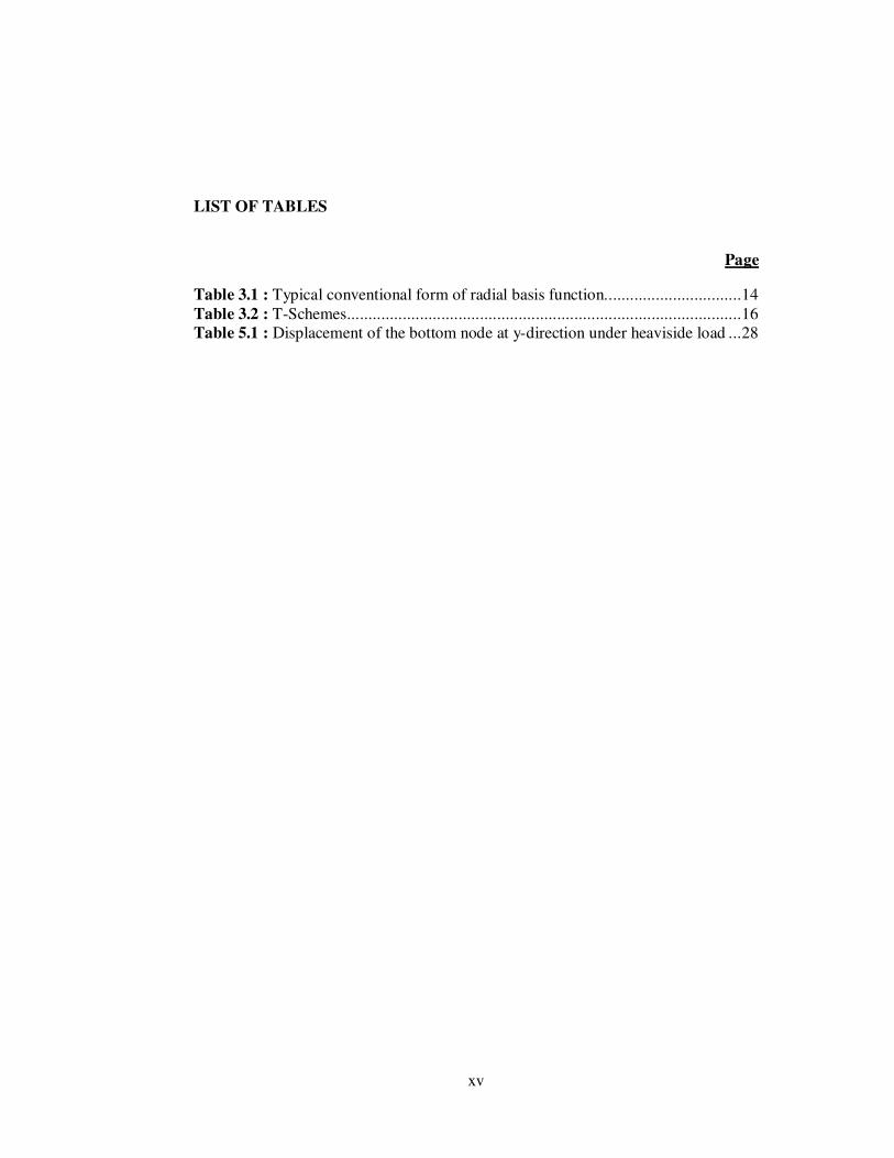
Table 3.1 : Typical conventional form of radial basis function. ............................... 14 Table 3.2 : T-Schemes............................................................................................ 16 Table 5.1 : Displacement of the bottom node at y-direction under heaviside load ... 28

xvi

xvii

LIST OF FIGURES

Page

Figure 1.1 : Comparision of FEM and Meshless Methods ....................................... 1 Figure 1.2 : Infinite space modelling. ...................................................................... 2 Figure 2.1 : Infinite region modelled by perfectly matched layer. ............................ 4 Figure 2.2 : Discretization of FEM and BEM. ......................................................... 4 Figure 2.3 : Introducing an artificial boundary into infinite domain. ........................ 6 Figure 2.4 : Mapping the solution in the analytic domain. ....................................... 6 Figure 2.5 : Solving the problem by mapping. ......................................................... 6 Figure 2.6 : Plane wave scheme on the artificial boundary. ..................................... 8 Figure 3.1 : Influence domains of nodes. ................................................................11 Figure 3.2 : T3 Scheme of node selection. ..............................................................17 Figure 3.3 : T6/3 Scheme of node selection. ...........................................................17 Figure 3.4 : T6 Scheme of node selection. ..............................................................18 Figure 3.5 : T2L Scheme of node selection for an interior and a boundary home

cell. .....................................................................................................18 Figure 3.6 : Illustration of edge-based (ES) smoothing domains. ............................22 Figure 3.7 : Sub domains and quadrature points for the mass matrix integration. ....23 Figure 4.1 : Flowchart of Matlab implementation. ..................................................25 Figure 5.1 : One dimensional column problem .......................................................27 Figure 5.2 : Displacement of center node along y-direction under impulse load......28 Figure 5.3 : Displacement of top node along y-direction under impulse load. .........29 Figure 5.4 : Displacement of center node along y-direction under heaviside load. ..29 Figure 5.5 : Displacement of top node along y-direction under heaviside load. .......30 Figure 5.6 : Displacement of bottom node along y-direction under impulse load. ...31 Figure 5.7 : Displacement of center node along y-direction under impulse load......31 Figure 5.8 : Displacement of top node along y-direction under impulse load ..........32

xviii

xix

EDGE-BASED SMOOTHED RADIAL POINT INTERPOLATION METHOD (ES_RPIM) FOR WAVE PROPAGATION PROBLEM

SUMMARY

In last decades, structural analyzes are playing major role for the mechanical design. Finite element method and meshfree methods are two common ways to simulate structural analyzes.

Meshfree methods are the alternative methods of finite element method. Although Finite element method has some advantages, Meshfree methods are choosen more often in order to compute the explicit dynamic analyzes. The computation of these methods are not stopped by more deformation because the Meshless Methods depend on node distribution basicly. In other words, there is no deformed element shape for the Meshless Methods. Types of the shape function computation determines the name of the meshfree methods. Several meshfree methods exist such as Element Free Galerkin (EFG) method, the Meshless Local Petrov-Galerkin (MLPG) method, the Point Interpolation method (PIM), Smoothed Particle Hydrodynamics (SPH) or Radial Point Interpolation method (RPIM). In this work, Edge-based Smoothed Radial Point Interpolation method is used to simulate wave propagation because of the non singularity moment matrix and patch test.

Wave propagation problem can be simulated by implementation of artificial boundary condition. Perfectly matched layer, boundary element method, infinite element method, Dirichlet-Neumann method and transmitting boundary method are the implementation ways of an artificial boundary. Because of the easy implementation, transmitting boundary method is selected in this work.

Abaqus and Matlab programs are used to simulate column model. Firstly, the results of Matlab program and Abaqus are compared to make sure that Matlab codes work true or not. Therefore, a column model with normal boundary conditions are prepared for a comparative study between Matlab and Abaqus. Left and right side of the model are constrained at x and z axis. All degrees of freedom are constrained at the bottom of the model. Impulse and heaviside forces are performed at the top of the model respectively. After the validation of Matlab model, the transmitting boundary method is implemented into Matlab. Transmitting boundary condition is only applied at the bottom. Displacements at the bottom, center and top nodes are observed. According to the results, the absorption is occured successfully.

xx

xxi

DALGA YAYILIMI PROBLEMĐNDE KENAR BAZLI YUMUŞATILMIŞ RADYAL NOKTASAL ENTERPOLASYON YÖNTEMĐNĐN

UYGULANMASI

ÖZET

Son yıllarda yapısal analizler mekanik tasarımlarda önemli bir rol üstlenmişlerdir. Tasarım hakkında fikir vermek amacıyla yapılan deneylerin yerini bilgisayar ortamında gerçekleşen analizler yer almıştır. Hazırlık süreci ve yapılan yatırımlar göz önüne alındığında bilgisayar ortamında yapılan analizlerin günümüzde daha fazla tercih edildiği görülmektedir. Yapılan analizlerin ışığında üretilen prototipler üzerinde yapılan testler bu analizlerin doğruluğunu kanıtlar niteliktedir. Sonlu elemanlar yöntemi ve ağsız yöntemler yapısal analizlerde kullanılan yaygın yöntemlerdir. Günümüzde sonlu elemanlar yöntemi kullanan birçok yazılım bulunmakla beraber ağsız yöntemleri kullanarak analiz gerçekleşen yazılımların sayısı da artmaktadır.

Ağsız yöntemler sonlu elemanlar yöntemine alternatif yöntem olarak ortaya çıkmıştır. Sonlu elemanlar methodunun birçok avantajları olmasına karşı ağsız yöntemler dinamik analizlerde daha sık tercih edilir. Aşırı deformasyon altında ağsız yöntemi kullanan modellerde analizlerde yakınsama problemi ile karşılaşılmaz. Çünkü bu yöntemler nokta dağılımına dayanarak çalışmaktadır. Sonlu elemanlar yönteminde ise model birden fazla elemanlardan oluştuğu için bu elemanlardan herhangi birisinde oluşacak aşırı deformasyon analizin durmasına ya da yakınsamamasına sebep olabilir. Başka bir deyişle aşırı deformasyonda şekil bozulmasına neden olabilecek elemanlar ağsız yöntemlerde tanınmaz. Bu yöntemlerde de sonlu elemanlar methodu gibi hesaplamaların yapılması için genelleştirilmiş katılık matrisi ve kütle matrisinin elde edilmesi gerekmektedir. Her iki yöntem için matrislerin oluşturulması aşamasında şekil fonksiyonları kullanılmaktadır. Ağsız yöntemlerin sonlu elemanlar methodundan farkı da bu noktada ortaya çıkmaktadır. Şekil fonksiyonunu, sonlu elemanlar methodunda modeli oluşturan eleman şekilleri belirlerken ağsız yöntemlerde ise modele dağılmış olan nokta bulutundan destek alanı oluşturarak hesaplanmaktadır. Şekil fonksiyonunu hesaplama yöntemi ağsız yöntemin adını belirlemektedir. Serbest eleman Galerkin yöntemi, lokal ağsız Petrov Galerkin yöntemi, nokta enterpolasyon yöntemi, yumuşatılmış parçacık hidrodinamiği yöntemi ve radyal nokta enterpolasyon yöntemi gibi birçok ağsız yöntem bulunmaktadır. Bu ağsız yöntemlerde sonlu elemanlar elemanlar methodu gibi benzer şekilde elde edilen şekil fonksiyonlarından genelleştirilmiş kütle ve katılık matrisleri oluşturulur. Sınır ve yükleme koşullarına bağlı olarak bu matrislerde eleminasyon gerçekleştirilir. Matris işlemleri yapılarak yerdeğiştirmeler elde edilmiş olur. Bu işlemlerinin arasında matrisin tersini alma gibi işlemlerde bulunmaktadır. Bu nedenle tekillik problemini önlemek amacıyla matrisleri oluşturan şekil fonksiyonları düzgün şeçilmelidir. Ayrıca modelde devamlılığı sağlamak da ağsız yöntemler ve sonlu elemanlar

xxii

methodu için önemli bir unsurdur. Sonlu elemanlar methodunda elemanlar birbiriyle bağlı olacak şekilde modelleme yapılarak bu sorun aşılırken ağsız yöntemlerde nokta bulutundan oluşturulan destek alanların birbiri ile bağlantışarı kontrol edilerek modelin devamlılığı sağlanmıştır. Bu çalışmada moment matrisinin tekillik hatası vermemesi ve şekil fonksiyonunun yama testini geçmesi nedeniyle kenar bazlı radyal nokta enterpolasyonu yöntemi ile dalga yayılımı simule edilmiştir.

Ağsız yöntemlerin genel formülasyonunda temel fonksiyon ve etki fonksiyonu olmak üzere iki fonksiyon bulunmaktadır. Temel fonksiyonun seçimi ağsız yöntemlerin özelliklerini belirlemektedir. Bu tezde radyal nokta enterpolasyonu yöntemi için multiquadratic, exponansiyel, ince plak eğrisi ve logaritmik olmak üzere 4 farklı temel fonksiyon belirlenmiştir. Bu temel fonksiyonların kullanıma uygun bir şekilde kod yazılarak numerik modelde esneklik sağlanmıştır.

Ağsız yöntemlerden radyal nokta enterpolasyon yönteminde dengeli ve doğru sonuç elde edebilmek için düzgün destek alanları elde etmek gerekmektedir. Bu nedenle de T şemalarından yararlanarak nokta seçimleri gerçekleştirilir. T3, T6/3, T6 ve T2L olmak üzere 4 farklı T şeması bulunmaktadır. T şema yöntemini kullanmak için model üzerinde sanki üçgen eleman varmış gibi noktalar dağıtılır. Destek alanının modelin sınırında ya da içerisinde oluşturulma durumuna bağlı olarak nokta seçimleri yapılır. Burada hangi T şemasının kullanılacağı belirtilir. T şemaları burada seçilecek nokta sayısını ve hangi noktaların seçileceğini belirlemek amacıyla kullanılır. Örneğin T3 şemasında model içerisinde veya sınırında toplam 3 adet nokta seçilmektedir. T6/3 şemasında ise model içerisinde seçim yapılırken 6, sınırdayken ise 3 adet nokta seçilmektedir. T6 şemasında model sınırı veya içerisinde 6 adet nokta seçilmektedir. Son olarak T2L şemasında ise farklı tabakalardan noktalar seçilerek destek alanı oluşturulmaktadır.

Dalga yayılımı problemi yapay sınır koşulları uygulanarak simule edilebilir. Bu sınır koşullarını oluşturabilmek için birçok yöntem kullanılmaktadır. Tabakalar arasındaki mükemmel uyum yöntemi, sınır eleman yöntemi, sonsuz eleman yöntemi, Dirichlet-Neumann yöntemi ve ileten sınır yöntemi yapay sınır koşulları uygulama yöntemleridir. Tabakalar arasındaki mükemmel uyum yönteminde sınıra yerleştirilmiş birden fazla tabakalarla ile sönümleme gerçekleştirilmeye çalışılmaktadır. Bu yöntemin işlem yükü oldukça ağır olması ve tam sönümlemenin sağlanamaması nedeniyle bu tezde tercih edilmemiştir. Sınır eleman yönteminde sadece modelin sınırlarına eleman ağı örülmektedir. Böylelikle işlem yükü hafifletilmiştir. Fakat modelin karmaşıklığına bağlı olarak bu yöntemde tekillik problemi ile karşılaşılabilinmektedir. Sonsuz eleman yönteminde ise bir elemanın sonsuz boyuta uzatılması prensibi kullanılmaktadır. Numerik hesaplamaların yapıldığı bu yöntemde karmaşık denklemlerin kullanılması nedeniyle işlem yükünün fazladır. Dirichlet-Neumann yönteminde model hesaplamalı alan ve analitik alan olmak üzere iki ayrı alt modele bölünür. Bu iki model arasında ortak sınır bulunmaktadır. Analitik alanda elde edilen veriler hesaplamalı alana sınır şartı olarak eklenerek çözümleme yapılır. Bu yöntem diğer yöntemlere göre daha dengeli ve doğru sonuçlar elde edilmesine karşı işlem yükü nedeniyle pek tercih edilmemektedir. Đleten sınır yönteminde ise geriye doğru enterpolasyon yöntemi kullanılarak yapay sınır şartları sağlanmaktadır. Sınırda bulunan noktalar kendilerinden bir önceki sırada bulunan noktalara bu enterpolasyon yöntemi ile bağlanmaktadır. Bu prensibe dayalı olarak ortaya çıkan enterpolasyon formülasyonu sayesinde sınırda yapay sınır koşulları sağlanarak sönümleme elde edilmektedir. Uygulanabilirliği kolay olduğu için ileten sınır yöntemi bu çalışmada seçilmiştir.

xxiii

Dalga yayılımı problemi zamana bağlı dinamik bir problem olduğu için zaman integresyonu olarak merkezi farklar methodu kullanılmıştır.

Matematik model Matlab programında kod yazarak oluşturulmuştur. Basit problem olması nedeniyle tek boyut olan kolon problemi seçilmiştir. Đlk olarak Matlab ve Abaqus'ten elde edilen sonuçlar karşılaştırılarak Matlab kodunun doğruluğundan emin olunmuştur. Bu yüzden kolon model oluşturularak Matlab ve Abaqus arasında karşılaştırma gerçekleştirildi. Öncelikle sonlu elemanlar methodu için Abaqus programında ve radyal nokta enterpolasyon yöntemi için ise Matlab programında aynı boyutta olacak şekilde geometrik model hazırlandı. Daha sonra malzeme özellikleri birim olarak her iki yöntem için belirlendi. Modelin sağ ve sol kenarlarında x ve z eksenlerindeki serbestlik dereceleri kısıtlanmıştır. Modelin alt kenarında ise tüm serbestlik dereceleri kısıtlanmıştır. Sırasıyla darbe ve birim yükleme durumunda model üzerindeki 3 farklı noktadaki yerdeğiştirmeler karşılaştırılmıştır. Darbe yükleme koşulu altında 3 farklı noktadan elde edilen yerdeğiştirme zaman grafikleri her iki yöntem için birbiriyle neredeyse uyum içinde olduğu farkedilmiştir. Abaqus programından elde edilen yerdeğiştirme grafiklerinde maksimum ve minimum bölgelerde salınımın olduğu gözlenmiştir. Bunun nedeninin zaman entegrasyon yönteminde belirlenen sönümleme katsayısının farklılığı olduğu bulunmuştur. Birim yükleme koşulu altında ise 3 farklı noktadan elde edilen yerdeğiştirme zaman grafikleri her iki yöntem içinde çok fazla benzerlik gösterdiği farkedilmiştir. Bu sonuçlara dayanarak Matlab programında hazırlanan matematik modelin doğruluğu sağlanmıştır. Dalga yayılımı problemini simule etmek için Abaqus programı tarafından doğrulanmış matematik model kullanılmıştır. Bunun için ileten sınır yöntemi Matlab koduna uyarlanarak model üzerinde alt, merkez ve üst noktadan yerdeğiştirmeler elde edilerek incelenmiştir. Hazırlanan bu ikinci örnekte yükleme koşulu olarak model üzerindeki sönümlemeyi incelemek için sadece darbe uygulanmıştır. Yükleme modelin üst sınırı boyunca uygulanmıştır. Ayrıca bu örnekte ilk örnekte olduğu gibi malzeme özellikleri birim olarak belirtilmiş olup geometrik özellikleri de aynı şekilde kalmıştır. Sadece modelin alt sınırına ileten sınır koşulları uygulanmış olup modelin sağ ve sol kenarlarındaki sınır koşulları ilk örnekte belirtildiği gibi bırakılmıştır. Bu şekilde darbe sonucu oluşacak dalga yayılımı tek yönlü olup y ekseni boyunca hareket etmesi amaçlanmıştır.

Sonuç olarak bu analiz neticesinde model üzerindeki elde edilen yer değiştirmeler ışığında sönümleme etkisinin oluştuğu farkedilmiştir. Modelin üst noktasında elde edilen yerdeğiştirme zaman grafiğinde analiz başlangıcında yükleme durumundan dolayı aşırı yer değiştirme gözlenmiş olup analiz boyunca yerdeğiştirmenin sıfır değerine yaklaştığı farkedilmiştir. Modelin orta noktasından elde edilen yerdeğiştirme zaman grafiğinde analiz başlangıcında üst noktaya göre daha az bir yerdeğiştirme gözlenmiş olup analiz boyunca yerdeğiştirmenin sıfır değerine yaklaştığı görülmüştür. Đleten sınır yönteminin kullanıldığı alt sınırdaki noktadan elde edilen yerdeğiştirme zaman grafiğinde ise yerdeğiştirmenin çok küçük olduğu ve analiz başlangıcında sıfırın etrafında salınım yapıp daha sonra sıfır değerine ulaştığı görülmüştür. Bu sonuçlar ışığında darbe sonucu oluşan dalganın ileten sınır yöntemi sayesinde sönümlemenin oluştuğu farkedilmiştir. Bir sonraki adım olarak elde bulunan matematik model geliştirilerek ileten sınır yönteminin iki ve üç boyutlu problemlere uyarlanması öngörülmüştür. Ayrıca ilk örnekte görülen Abaqus ve Matlab programlarında elde edilen sonuçlar arasındaki küçük farkların nedeninin araştırılması ve zaman entegrasyonunda belirlenen sönümleme katsayılarının bu sonuçlara olan etkisinin incelenmesi de bir sonraki adım olarak belirlenmiştir.

xxiv

1

1. INTRODUCTION

In standard numerical methods, as in finite element method (FEM), finite difference

method (FDM) and finite volume method (FVM), a mesh must be predefined to

provide a connectivity between the nodes. The system equation is formed by

assemblying the elements’ equations, which keeps the computational times low. In

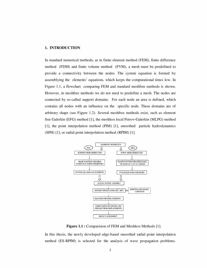
Figure 1.1, a flowchart comparing FEM and standard meshfree methods is shown.

However, in meshfree methods we do not need to predefine a mesh. The nodes are

connected by so-called support domains. For each node an area is defined, which

contains all nodes with an influence on the specific node. These domains are of

arbitrary shape (see Figure 1.2). Several meshfree methods exist, such as element

free Galerkin (EFG) method [1], the meshless local Petrov-Galerkin (MLPG) method

[1], the point interpolation method (PIM) [1], smoothed particle hydrodynamics

(SPH) [1], or radial point interpolation method (RPIM) [1].

Figure 1.1 : Comparision of FEM and Meshless Methods [1].

In this thesis, the newly developed edge-based smoothed radial point interpolation

method (ES-RPIM) is selected for the analysis of wave propagation problems.

2

This method is based on a weakened weak formulation, allowing the adoption of a

nodal integration scheme, which reduces the computational times

considerably in comparison with the Gauss quadrature method.

Wave propagation problems are defined on infinite domains. In the

numerical simulation the problem domain has to be bounded, though. To

keep the computational effort low only the region of interest is discretized (see

Figure 1.2). To avoid reflections, wave absorbind or transmitting boundary

conditions are applied. Different methods for modelling infinite domains exist, as

for example perfectly matched layers (PML), boundary element method (BEM),

infinite element method (IFEM), viscous boundary conditions, the dirichlet to

neumann method (DtN) and transmitting boundary method, which are explained in

the following.

Figure 1.2 : Infinite space modelling [2].

3

2. INFINITE DOMAIN MODELLING

Unbounded domain is generally used in engineering and scientific applications,

such as earthquake simulations, radar technology, acoustic problems and fluid

dynamics. In order to model the infinite domain, local domain is constructed in

the infinite domain and the boundaries of local domains are simulated like

the artificial boundary.

2.1 Alternative Methods

For the infinite domain modelling, different numerical methods, which are

expressed the next sections, exist. These alternative methods aim to simulate

the artificial boundary conditions.

2.1.1 Perfectly matched layer

A perfectly matched layer (PML) is an artificial absorbing layer for wave

equations. The boundaries of a truncated region are enclosed by such perfectly

absorbing layers not to allow reflections back into the domain. The waves are

transmitted completely into the PML and oscillate between the outer boundary and

the interface until they decay (see Figure 2.1). The following characteristics of

PMLs emerge:

• Since the formulation depends on the frequency, the implementation in

time domain is rather complex.

• Small reflections do occur, because of the discretization of the wave

equation.

This can be handled by tuning the absorption parameter.

• Many enhancements of PMLs exist, which are able to treat waves hitting

the interface under a certain angle and transverse modes.

• It is not possible to model inhomogeneous media with PMLs in general.

4

Figure 2.1 : Infinite region modelled by perfectly matched layer [4].

2.1.2 Boundary element method

The boundary element method (BEM) is a numerical computational method

for solving partial differential equations. However, there are some differences

regarding the other numerical methods. For instance, in BEM only the boundaries

have to be discretised (see Figure 2.2). Depending on the complexity of

geometric model and load case, BEM provides time saving. Generally, this method

is used for computing the stress concentration in infinite and semi infinite domains.

Figure 2.2 : Discretization of FEM and BEM [1].

Advantages and disadvantages of boundary element method are stipulated below:

+ Only the boundary is discretised in the boundary element method.

+ The accuracy of the stress distribution problem is improved.

+ Simple and accurate model is obtained.

− Non symmetric system of equations.

− Requires the knowledge of suitable fundamental solution.

5

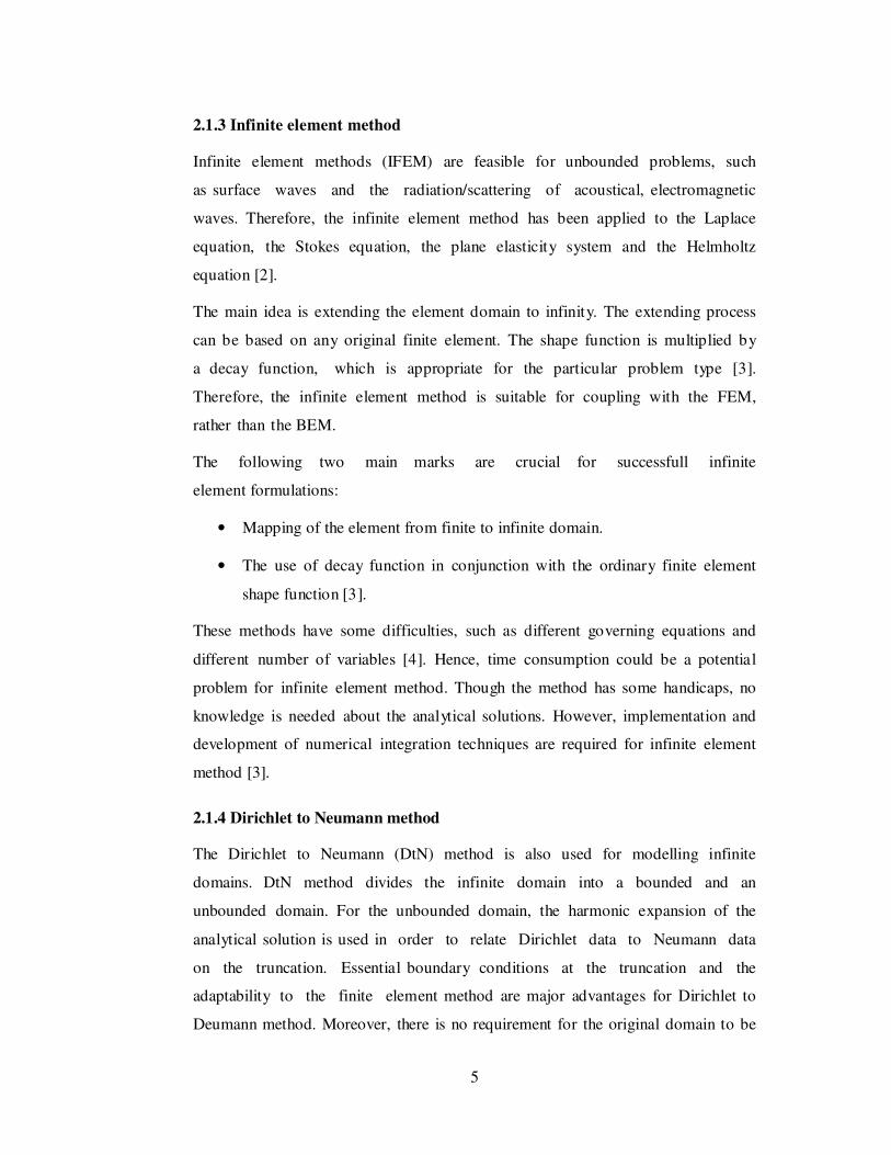
2.1.3 Infinite element method

Infinite element methods (IFEM) are feasible for unbounded problems, such

as surface waves and the radiation/scattering of acoustical, electromagnetic

waves. Therefore, the infinite element method has been applied to the Laplace

equation, the Stokes equation, the plane elasticity system and the Helmholtz

equation [2].

The main idea is extending the element domain to infinity. The extending process

can be based on any original finite element. The shape function is multiplied by

a decay function, which is appropriate for the particular problem type [3].

Therefore, the infinite element method is suitable for coupling with the FEM,

rather than the BEM.

The following two main marks are crucial for successfull infinite

element formulations:

• Mapping of the element from finite to infinite domain.

• The use of decay function in conjunction with the ordinary finite element

shape function [3].

These methods have some difficulties, such as different governing equations and

different number of variables [4]. Hence, time consumption could be a potential

problem for infinite element method. Though the method has some handicaps, no

knowledge is needed about the analytical solutions. However, implementation and

development of numerical integration techniques are required for infinite element

method [3].

2.1.4 Dirichlet to Neumann method

The Dirichlet to Neumann (DtN) method is also used for modelling infinite

domains. DtN method divides the infinite domain into a bounded and an

unbounded domain. For the unbounded domain, the harmonic expansion of the

analytical solution is used in order to relate Dirichlet data to Neumann data

on the truncation. Essential boundary conditions at the truncation and the

adaptability to the finite element method are major advantages for Dirichlet to

Deumann method. Moreover, there is no requirement for the original domain to be

6

homogeneous and isotropic. Although, the accuracy and the stability of the results

are so high, the computation is very hard, because of multiple integrations over

the truncation, complex and extensie block [5] at the resulting system and the low

efficiency of finite element solvers.

The DtN method can be defined in four steps [6]. They are described at below.

Step 1: Introduce the artificial boundary B, dividing the infinite domain Ω into the

computational domain and the analytic domain (see Figure 2.3).

Figure 2.3 : Introducing an artificial boundary into infinite domain [4].

Step 2: Solve the problem in the analytic domain to provide felicitous relation

between the unknown variable and its derivative on the artificial boundary

(see Figure 2.4).

Figure 2.4 : Mapping the solution in the analytic domain [4].

Step 3: Apply the felicitous relation as a boundary condition on the artificial

boundary.

Step 4: Solve the problem in the computational domain (see Figure 2.5).

Figure 2.5 : Solving the problem by mapping [4].

7

2.1.5 Transmitting boundary method

The transmitting boundary method is based on defining an artificial boundary and

introducing a numerical method for transmitting waves out of an artificial

boundary. An extrapolation formula is used for describing the numerical method.

Therefore, the implementation of the method is uncomplicated and it cooperates

with the finite element method, finite difference method or meshfree method. The

accuracy of the method depends on the number of terms in the extrapolation series

and the choice of the time step size.

In this thesis, because of simple implementation process and excellent accuracy

of the artificial boundary, transmitting boundary method is chosen in order to

model the infinite domain. The theory of the method is explained in details at the

next section (2.2).

2.2 Transmitting Boundary Condition

Wave propagation problems can be simulated by using the artificial

boundary conditions. During the simulation, the motion equation is used. At this

equation, the stiffness matrix couples a particular node to its adjacent nodes

from all sides. However, for the artificial boundary nodes the stiffness matrix

does not couple the exterior nodes [7]. Transmitting boundary formula is

aimed to overcome this problem by using one side of a particular node.

In order to assume one-sided formula, a linear wave field is represented by a

plane wave expansion [7].

U ( x, y, z, t) = ∑ui (ξi − ct) (2.1)

Where ui (ξi − ct) is a plane wave which is traversing in positive ξi direction with a

physical velocity of c.

The schematic of a plane wave is demonstrated in Figure 2.6. The point P is a

node which is on the artificial boundary and the x-axis is the normal axis to the

artificial boundary. At point P, the displacement for the time step t+∆t is mentioned

in Equation 2.2.

8

u[ξ p

− c(t + ∆t)] = u[(ξ p

− c∆t) − ct] = u[(ξ p

− 2c∆t) − c(t − ∆t)] (2.2)

All terms in equation 2 have different physical meanings although their numerical

values of the argument are equal [7]. For time step t, the point E is located ξp-c∆t

on the ξ axis because the plane wave travels c∆t in one time step. For time step t-∆t,

the point E is located ξp-2c∆t on the ξ axis. In Figure 2.6, the solid and dashed

lines for time step t and t-∆t respectively determined the point E on the ξ axis.

Instead of the ξ axis, the x axis is used for observing the plane waves because ξi

directions are not available for the plane waves. The velocity on the x axis (CI) is

defined at Equation 2.3.

cos⁄ (2.3)

On the x axis the points E are located at distance in multiples of CI∆t from xp. The

value of CI∆t is an unknown value for each plane wave. Therefore, the distances

between points are assumed multiples of d from P on the x axis.

Figure 2.6 : Plane wave scheme on the artificial boundary [7].

The amplitudes at any two points on the wave are equal if the plane wave is one

dimensional [7]. The amplitude at xp-d on the ξ axis and at point A0 is the same.

Location of A0 on the ξ axis is computed by Equation 2.4.

ξ cosθ ξ d (2.4)

9

where ξp is the location of P on the ξ axis.

The distance between A0 and E points is ε0 which is defined in Equation 2.5.

∆ (2.5)

For each time step, the amplitude on the ξ axis and the x axis must be equal. On the ξ

axis, the distance between point E and A-m is (m-1) ε0.

In order to obtain the amplitude at point E, the approximation amplitude (A-m) is fine

prediction. However, an extrapolation method can be implemented by using the

collection of all amplitudes at A-m.

, , , + ∆ + ∆"+. . . +∆$ + 0&$'( (2.6)

where

∆) ∆)*( ∆)*(*( (2.7)

Assumption of d is affected from the accuracy of the extrapolation method. In order

to obtain more accurate results, ε0 should approach to zero. Therefore, d can be

chosen near the value CI∆t. On the other hand, according to numerical experiments, d

is chosen near shear velocity (Cs) for SH wave problems [7].

In this work, extrapolation method is used to obtain the displacement at the artificial

boundary nodes.

10

11

3. MESHFREE METHODS

In meshfree methods nodes are distributed at the problem domain arbitrarily. Shape

functions are generated by using predefined support domains [1]. In this work, the

radial point interpolation method (RPIM) is applied. The construction of the shape

function is explained in Section 3.1.

The support domain for a point xQ can be determined by defining a support radius:

+ ,+ - (3.1)

The coefficient αs is a measure for the average nodal spacing. The principle is

displayed in Figure 3.1. Alternatively, the influence domain principle could be used

or the support nodes can be selected by using a T-scheme, which is adapted in this

work and described in detail in Section 3.2.

For constructing the system matrices, the generalized smoothed Galerkin weak form

of Eulers equation of motion is derived in Section 3.3. Edge based smoothing

domains are adopted. A lumped mass matrix enables the employment of the explicit

time stepping procedure (Section 3.4).

Figure 3.1 : Influence domains of nodes [1].

12

3.1 Meshfree Shape Function

The construction of the shape function plays a major role in Meshfree methods. In

order to obtain the efficient accuracy in the problem domain, some conditions, such

as an arbitrary nodal distribution, the stable algorithm, consistency of the shape

function construction, the compact support or influence domain, an efficient

computation for the shape function construction, the satisfaction of the Kronecker

delta function property and the existence of the compatible shape function, are

required [1]. Therefore, the radial point interpolation method (RPIM), which was

developed, is chosen to construct the shape function in this work.

The point interpolation methods are based on interpolation function which is

obtained by the function values of the arbitrary nodes in the support domain. The

following finite series representation is the beginning of point interpolation methods

formulations [1]:

./, 0 12345630 738( (3.2)

where n is the number of nodes in support domain of point xQ, Bi(x) are the basis

functions in the Cartesian coordinates, ai(xQ) are the factor of the basis function.

According to forms of basis functions, polynomial and radial point interpolation

methods are existed. In the polynomial point interpolation method, Pascal triangle is

used as a basis function.

The general form of the polynomial point interpolation method:

./, 0 1345738( 630 94560 (3.3)

where pT(x) is basis function of the point interpolation method. For instance one and

two dimensional of polynomial basis functions are:

945 :1, , ", <, ……… , 7> (1D) (3.4)

13

94, 5 :1, , , , ", ", ……… , 7, 7>42@5 (3.5)

Equation 3.3 can be written in matrix form.

A+B CD0EA6B (3.6)

The values of the field variables, at the all nodes in the support domain, are included

in Us vector. PQ is the moment matrix.

To obtain coefficient of basis function, Equation 3.6 is multiplied by inverse of the

moment matrix:

A6B CD0E*(A+B (3.7)

To construct the shape functions, substituting Equation 3.7 into Equation 3.2:

./45 F45+ (3.8)

where Φ(x) is the matrix of point interpolation shape functions.

F45 945D0*( (3.9)

Equation 3.9 shows that the moment matrix must be invertible to construct the shape

functions. Therefore, the form of the basis function is determinant for the moment

matrix.

In radial point interpolation method, the shape functions are obtained by using the

radial basis functions to prevent the singularity problem at the moment matrix [1].

The general form of the radial interpolation method:

./, 0 1G345738( 630 G94560 (3.10)

where RT(x) is the radial basis functions.

Many radial basis functions are existed. Four often use forms of radial shape

functions with some shape parameters are listed in Table 3.1. [1].

14

Table 3.1 : Typical conventional form of radial basis functions [1].

Items Name Expression Shape Parameters

1 Multiquadratics (MQ) G34, 5 4H3" + "5I C,q

2 Gaussian (EXP) G34, 5 J4H3"5 C

3 Thin plane spline (TPS) G34, 5 H3K L

4 Logaritmic (RBF) G34, 5 H3KMNOH3 L

In order to construct the ideal shape functions, the consistency of the basis function is

as sufficient as the invertible moment matrix to pass the standard patch test [1].

Therefore, in the radial point interpolation method (RPIM), radial and polynomial

basis functions are used all together for the construction of the shape functions to

create the nonsingular moment matrix and provide consistency of the shape

functions.

./, 0 ∑ G345738( 63 +∑ 345QR)R8( G9456 + 945b (3.11)

where n is the number of nodes of the basis function in the support domain, m is the

number nodes of the polynomial basis function, Ri(x) is the radial basis function with

r distance between x and xi, ai is the coefficient of the radial basis function, pi(x) is

the polynomial basis function, bj is the coefficient of the polynomial basis function.

The vector forms of a and b are:

6 :6( , 6" , 6< , ……… , 67> (3.12)

Q :Q( , Q", Q<, ……… , Q)> (3.13)

The vector forms of RT(x) and pT(x) are:

G945 :G(45, G"45, G<45, ……… , G745> (3.14)

945 :(45, "45, <45,……… , )45> (3.15)

15

Equation 3.11 can be written in matrix form:

:+> CG0EA6B + :D)>b (3.16)

where Us is the vector which collects the field variable of n nodes in the support

domain. In Equation 3.16, polynomial term (Pm) ensures the reproduction of

consistency [1]:

:D)>9A6B 0 (3.17)

Combination of Equation 3.16 and 3.17 is

SG0 D)D)9 0 T U6QV U+0 V (3.18)

The coefficient of radial basis function (a) can be obtained in Equation 3.16:

A6B CG0E*(A+B CG0E*(:D)>AQB (3.19)

Substituting Equation 3.19 into 3.17.

AQB :WX>A+B (3.20)

Where Sb is

WX CD)9G0*(D)E*(D)9G0*( (3.21)

The interpolation can be written as

.45 :G945WY + 945WX>+ F45+ (3.22)

where Φ(x) is the matrix of the shape functions of the radial point interpolation

method:

F45 :G945WY + 945WX> :∅(45, ∅"45, ∅<45,……… ,∅7> (3.23)

16

For instance, the shape function of ith node (φi (x) ):

∅345 1G345W3[Y7

38( +1RWR[X)R8( (3.24)

The shape function are derived easily:

\∅[\ 1\G3\ W3[Y + 1\R\ WR[X)R8(

738( (3.25)

\∅[\ 1\G3\ W3[Y + 1\R\ WR[X)R8(

738( (3.26)

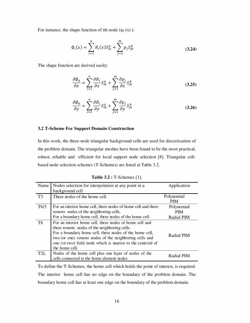
3.2 T-Scheme For Support Domain Construction

In this work, the three-node triangular background cells are used for discretization of

the problem domain. The triangular meshes have been found to be the most practical,

robust, reliable and efficient for local support node selection [8]. Triangular cell-

based node selection schemes (T-Schemes) are listed at Table 3.2.

Table 3.2 : T-Schemes [1].

Name Nodes selection for interpolation at any point in a background cell

Application

T3 Three nodes of the home cell. Polynomial PIM

T6/3 For an interior home cell, three nodes of home cell and three remote nodes of the neighboring cells. For a boundary home cell, three nodes of the home cell.

Polynomial PIM

Radial PIM T6 For an interior home cell, three nodes of home cell and

three remote nodes of the neighboring cells. For a boundary home cell, three nodes of the home cell, two (or one) remote nodes of the neighboring cells and one (or two) field node which is nearest to the centroid of the home cell.

Radial PIM

T2L Nodes of the home cell plus one layer of nodes of the cells connected to the home element nodes

Radial PIM

To define the T-Schemes, the home cell which holds the point of interest, is required.

The interior home cell has no edge on the boundary of the problem domain. The

boundary home cell has at least one edge on the boundary of the problem domain.

17

In T3 Schemes, three nodes are selected even if the home cell is an interior or a

boundary home cell (Figure 3.2). Cell i and Cell j are an interior home cell and a

boundary home cell respectively. In order to create linear PIM shape function, T3

scheme is used. The moment matrix is always an invertible matrix [9]. Therefore, the

shape functions are always constructed.

Figure 3.2 : T3 Scheme of node selection [1].

In T6/3 Scheme, six nodes are selected from an interior home cell and three nodes

are selected from a boundary home cell (Figure 3.3).

Figure 3.3 : T6/3 Scheme of node selection [1].

Passing the standard patch test is guaranteed by using T6/3 Scheme, because of using

three nodes for the boundary home cell.

In T6 Scheme, three nodes of home cells and three nodes of neighboring cells are

selected for an interior home cell. For a boundary home cell, three nodes of home

cells, two nodes of neighboring cells and one field node, which is the nearest node of

centroid of the home cells, are selected (Figure 3.4).

18

Figure 3.4 : T6 Scheme of node selection [1].

T6 Scheme of node selection is used for constructing radial point interpolation

method shape functions.

In T2L Scheme, two layers of nodes are selected to interpolate according to

triangular meshes. Three nodes of home cells are obtained the first layer. The nodes,

which are directly connected with the nodes at first layer, are obtained the second

layer. In Figure 3.5, T2L Scheme is demonstrated for an interior home cell and a

boundary home cell.

Figure 3.5 : T2L Scheme of node selection for an interior and a boundary home cell [1].

In T2L Scheme, more nodes can be selected than in T6 Scheme. Therefore, time

consuming is a problem for this scheme. T2L scheme is used for creating the radial

shape functions of extremely irregularly scattered nodes.

19

3.3 Generalized Smoothed Galerkin Weak Form

The basic momentum balance equations are given for the two dimensional solid

dynamics.

]9_ + Q `4.a O5 (3.27)

]9_ + Q `4.a O5 (3.27)

where b is the body force, ρ is the specific weight, g is the gravity and Ld is the

differential editor.

]^ bcccccd \\ 00 \\\\ \\eff

fffg (3.28)

Strains are obtained by multiple of Ld and displacements.

]^. (3.29)

where Ch , i , hiE9and . C.h , .iE9 .

Generalized weak form is used for computing the Cauchy stresses.

_ (3.30)

where

j41 + k541 2k5 l1 k k 0k 1 k 00 0 1 2k2 m (3.31)

20

For the plane strain condition:

j41 k"5 l1 k 0k 1 00 0 1 k2 m (3.32)

Where E is Young modulus and υ Poisson’s ratio.

In order to obtain the exact solution, Dirichlet (essential) and Neumann (natural)

boundary conditions have to be applied:

. .& Nnop4@qHqℎMJ5 (3.33)

]79_ &Nnos 4tJ.u6nn5 (3.34)

The Galerkin weak form depends on the weighted residual method. During the

substituting Equation 3.2 into Equation 3.27, the residual will exist. Therefore, a

suitable weighted function is used to cancel out the residual:

v wC]9]^F `F Oa Ex y 0 (3.35)

According to divergence theorem:

v w]9_ y v w]79_ zx o v ]9w_ x y (3.36)

The divergence theorem is applied to Equation 3.35.

v C4]^F59]^F +F9`Fa Ex y v F94Q + `O5x y +v F9]79_ oz (3.37)

Strain matrix is defined as

2 ]^F :2(, 2", 2<, ……… , 27> (3.38)

21

i

2[ bcccccd\∅[\ 0

0 \∅[\\∅[\ \∅[\ efffffg, 1,2,3,……… , n+ (3.39)

Equation 3.37 is arranged like

a + ~ (3.40)

Where

v F9`F yx (3.41)

~ v 292 yx (3.42)

v F94Q + `O5 y +v F9zx o (3.43)

In this work, the strains will be obtained by using generalized smoothed galerkin

weak form. The reason is preventing the discontinuous displacements function which

is caused by the radial point interpolation shape functions [9].

Generalized smoothed galerkin weak form based on dividing problem domain into

smoothing domains with areas ( As ). Delaunay triangulation is used for the

construction of areas. Firstly, triangular background cells discretize the problem

domain and then the smoothing domains are constructed by these triangles [10].

Edge-based (ES), nodal-based (NS) and cell-based (CS) smoothing domains are

existed. In this work, edge-based smoothing domains are used (Figure 3.6).

22

Figure 3.6 : Illustration of edge-based (ES) smoothind domains [9].

In ES-RPIM, the smoothing domains are constructed with respect to the edges of the

triangular cells by connecting two ends of the edges of two adjacent cells [9].

In edge-based smoothing domains, the strains are defined:

& 13+ v 2 y 13+ v ]7F o 13+z 1R]7FR 738(x (3.44)

Using the strain values in Equation 3.44 instead of in Equation 3.29, stiffness matrix

in Equation 3.42 is defined as

~ 13+292$38( (3.45)

Where

2 13+ 1R]77R8( FR (3.46)

The local stiffness matrices, which are computed by generalized smoothed galerkin

weak form, are assembled to obtain global stiffness matrix.

In order to compute the mass matrix and the body force vector, a nodal quadrature

scheme, such as a stress point integration scheme can be applied. A stress point

integration scheme is based on adding quadrature points which are the centers of the

23

Delaunay triangles [10]. Therefore, the efficiency of the dynamics analyzes is

increased by a new quadrature scheme. On the other hand, the shape functions and

the guadrature weights are computed at once.

Figure 3.7 : Sub domains and quadrature points for the mass matrix integration [9].

The mass matrix is defined

13F&9$38( 435`F435 (3.47)

Where 3+ the weight area and t is the total number of quadrature points.

3.4 Central Differences Method

Explicit and implicit time integrations are two different approaches to solve the

system equations. Dynamic analyzes, in which the displacements are a function of

time, solved by explicit time integration. Therefore, in this work the system

equations of the problem are solved by central differences method, which is explicit

time integration.

General system equation for the dynamic analyzes is :

sa + s + ~s s (3.48)

In the central differences method, acceleration is assumed for the time t that,

24

sa 1∆" 4s*∆s 2s + s'∆s5 (3.49)

The velocity equation is defined as

s 12∆ 4s*∆s + s'∆s5 (3.50)

Substituting Equation 3.49 and 3.50 into Equation 3.48, to obtain displacement at

time t+∆t

1∆" + 12∆s'∆s s ~ 1∆"s 1∆" 12∆ s*∆s (3.51)

In central difference method, lumped mass matrix is implemented to reduce the

computation of system equations. On the other hand, in order to obtain the efficient

accuracy, a small time step size is assumed. Time step size must be smaller than the

critical values [6].

∆ ≤ ∆- 7 (3.52)

25

4. IMPLEMENTATION INTO MATLAB

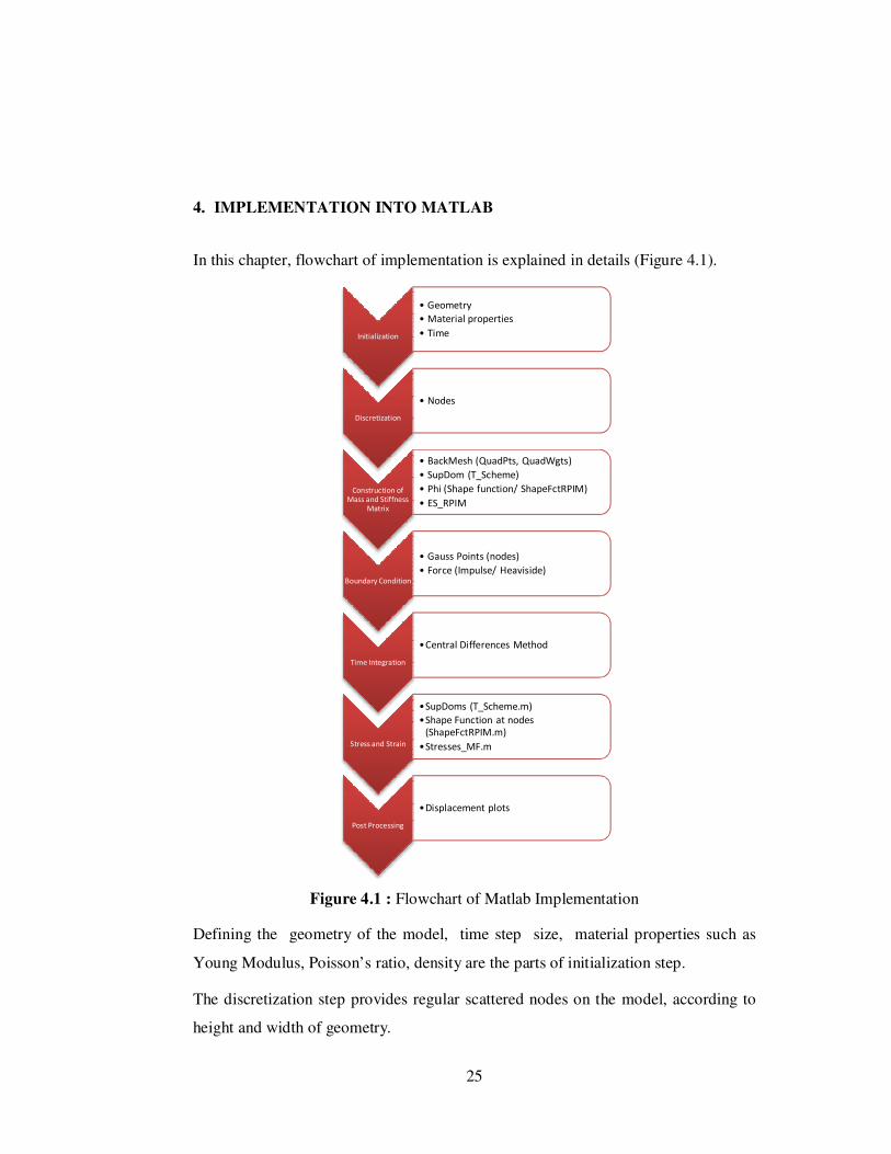
In this chapter, flowchart of implementation is explained in details (Figure 4.1).

Figure 4.1 : Flowchart of Matlab Implementation

Defining the geometry of the model, time step size, material properties such as

Young Modulus, Poisson’s ratio, density are the parts of initialization step.

The discretization step provides regular scattered nodes on the model, according to

height and width of geometry.

Initialization

• Geometry

• Material properties

• Time

Discretization

• Nodes

Construction of Mass and Stiffness

Matrix

• BackMesh (QuadPts, QuadWgts)

• SupDom (T_Scheme)

• Phi (Shape function/ ShapeFctRPIM)

• ES_RPIM

Boundary Condition

• Gauss Points (nodes)

• Force (Impulse/ Heaviside)

Time Integration

•Central Differences Method

Stress and Strain

•SupDoms (T_Scheme.m)

•Shape Function at nodes

(ShapeFctRPIM.m)

•Stresses_MF.m

Post Processing

•Displacement plots

26

After the discretization, nodes are used in Backmesh m-file to obtain quadratic points

and quadratic weights. To define a support domain, nodes of the model, the quadratic

points and types of support domain determination are necessary for T-Scheme m-file.

After that, support domain, quadratic points and nodes of the model are used in

ShapeFctRPIM m-file to obtain radial point interpolation shape functions. All inputs

are ready for the mass matrix construction. On the other hand, material matrix and

nodes of the model are used in ES_RPIM m-file to construct stiffness matrix.

Boundary conditions are implemented by eliminating some rows and columns from

the mass and stiffness matrix. Moreover, in order to apply impulse and Heaviside

force on the upper boundary, gauss weights, gauss points and determinant of

jacobian of given order for a node structure rectangular cells are computed by

GaussPoints m-file. In addition, artificial boundary nodes are determined to be ready

for the time integration step.

During time integration, displacements of the nodes are computed by central

differences method and backward extrapolation method. For the artificial boundary

nodes, only initial displacements are computed by central differences method. In

other steps, displacements are computed by backward extrapolation method to

simulate the transmitting boundary condition.

Central differences method is always used to compute the displacements of the other

nodes.

According to displacements, stresses and strains are able to be computed by

Stresses_MF m-file. During this process, shape function and support domain of the

nodes are also required.

27

5. NUMERICAL EXAMPLES

5.1 Dynamic Analysis With Newmark Method in One Dimensional Column

Column model is the easiest model to compute numeric analyzes. Therefore, a

column model is set in order to compare the FEM results and RPIM results. Abaqus

is used to generate a Finite element model. For the Meshfree model, Matlab

computes the numerical analyzes.

The force is applied the whole upper boundary nodes and the bottom boundary is

behaved like an encastre boundary. Left and right side boundaries only allow moving

along y-direction (Figure 5.1).

Figure 5.1 : One dimensional column problem.

The mechanical properties of soil and the measurements of the model are given at

Table 5.1.

28

Table 5.1 : General properties of column model.

Height 10 Width 2 Pressure 1 Young Modulus 1 Poisson’s Ratio 1 Pressure 1

According to the load types, two column models are set for the problem. At the first

model, an impulse load is applied to the upper boundary of the model. During the

comparision, the results are obtained from three nodes respectively bottom node,

center node and top node on the model. Displacement values of the bottom node are

equals to zero because of the encastre boundary condition. Displacements of the

center node and top node along y-direction are shown at Figure 5.2, Figure

5.3 respectively.

Figure 5.2 : Displacement of center node along y-direction under impulse load.

29

Figure 5.3 : Displacement of top node along y-direction under impulse load.

Instead of the impulse load, the heaviside load is applied at whole upper boundary

in order to set the second model. Under the heaviside load, displacements of

center node and top node are shown at Figure 5.4 and Figure 5.5 respectively.

Figure 5.4 : Displacement of center node along y-direction under heaviside load.

30

Figure 5.5 : Displacement of top node along y-direction under heaviside load.

According to the comparision between Matlab and Abaqus results, under the same

boundary conditions, the meshfree model has the same behaviours like FEM model.

Therefore, the meshfree model can be used to simulate wave propagation problem.

5.2 Wave Propagation in One Dimensional Column

In order to simulate the artificial boundary conditions, the transmitting boundary

method is implemented into the present matlab code. Moreover,only bottom of the

model is behaved like an artificial boundary. The other boundary conditions are the

same like previous model. On the other hand, only impulse load is applied at whole

upper boundary nodes. During the initialization step, time is determined like 1000

sec and the number of time step is 1001. The same mechanical properties and

measurements are implemented in order to simulate wave propagation problem in

one dimensional column.

At this model, the displacement values are also obtained from three nodes such as

bottom node, center node and top node on the model respectively. Displacements of

the bottom node are shown at Figure 5.6.

31

Figure 5.6 : Displacement of bottom node along y-direction under impulse load.

Figure 5.7 : Displacement of center node along y-direction under impulse load.

32

Figure 5.8 : Displacement of top node along y-direction under impulse load.

33

6. CONCLUSION

In conclusion, one dimensional column problem is simulated at Abaqus program. On

the other hand, the same model is implemented into Matlab. When impulse load is

applied, displacement of the center node and top node are oscillated at x-axis. Under

the Heaviside load, displacement of the center node and top node are negative values.

Displacement of the bottom node always equals to zero because the bottom boundary

behave encastre under two load types (impulse and heaviside). The similar results are

obtained from Matlab program and Abaqus program. Therefore, for the column

model the artificial boundary conditions are implemented into the Matlab code.

The bottom of the model behave like an artificial boundary. The results show that the

transmitting boundary method works well because absorbing is observed at bottom,

center and top of the model. Under the impulse load condition, displacement of the

bottom node is oscillating at x-axis. After a while, absorption occurs and

displacements of the bottom node equals to zero. On the other hand, displacement

plot of the center node shows the effects of the artificial boundary because at the end

of the analysis, displacement values are nearly zero. For the top node, at the

beginning of the analysis displacement values are negative. However, at the middle

of the analysis, it equals to zero. According to these plots, we can say that artificial

boundary conditions are simulated successfully.

For the next step, two or three dimensional problem can be implemented into Matlab

code. The other infinite domain modeling method can be critised.

34

35

REFERENCES

[1] Liu, G. R. ( 2003). Meshfree Methods. National University of Singapore, Singapore.

[2] Li,L-X. Kunimatsu, S. Wang A-Q. : Application of the generalized infinite

element method to unbounded elastostatic problems. Jiatong University,China.

[3] Bettess, P. (1992). Infinite Elements. Page 25-28, Newcastle, United Kingdom. [4] Lungan, Y. (2001). Infinite element method for problems on unbounded and

multiply connected domains/ School of Mathematics Science, Peking University.

[5] Bergen, B. Vangenechten, B. Vandepitte, D. Desmet, W. (2010). An

explicit wave based finite element model as alternative to DtN finite element method. Belgium.

[6] Bathe, K.J. (1996). Finite Element Procedures. New Jersey, USA.

[7] Liao, Z. P. Wong,H. L. (1984). A transmitting boundary for the numerical simulation on elastic wave propagation. Academia Sinica, Harbin, China, University of Southern California, Los Angeles, USA.

[8] Liu, G. R., Zhang, G. Y., Dai, K. Y., Wang, Y. Y., Zhong, Z. H., Li, G. Y., Han, X. (2007). A linearly conforming point interpolation method (LC-PIM) for 2D mechanics problems. National University of Singapore, Singapore.

[9] Liu, G. R., Zhang, G. Y. (2008). Edge based smoothed point interpolation methods.National University of Singapore, Singapore.

[10] Soares, Jr. D., Schoenewald, A., Estorff, O. ( 2011). An efficient smoothed point interpolation method for dynamic analyses. Hamburg University of Technology. Hamburg, Germany.

36

37

APPENDICES

APPENDIX A.1 : Script_Structure.m (Matlab Subroutine)

APPENDIX A.2 : CentralDiff.m (Matlab Subroutine)

38

39

APPENDIX A.1

clear all, close all, format long %% Initialisation *********************************************************

Lx=2; Ly=10; % Width Lx, Height Ly x0=0;x1=2; % Area where load is applied nx=7;ny=31; % Number of elements in x and y sigma0=-1; % Constant pressure T=100; % Maximum time Nt=1001; % Number of time steps nu=0.3; % Poisson's ratio E=1; % Yield modulus

rho=1; % Density %------------------------------------------------------------------- ------- % Computing additional parameters t=linspace(0,T,Nt); % Discrete time vector h=sqrt((Lx/(nx-1))^2+(Ly/(ny-1))^2); % Nodal spacing %% Discretisation ********************************************************* % Create uniformly spread nodes grdx=linspace(0,Lx,nx); grdy=linspace(0,Ly,ny);[xe,ye]=meshgrid(grdx,grdy); nodes=[xe(:),ye(:)]; N=size(nodes,1); %% Construction of mass matrix ******************************************** [QuadPts,QuadWgts] = BackMesh(nodes,5); % Background Mesh: equ.sh.SPI SupDom = T_Scheme(nodes,QuadPts,4); % Support domain: T6- Scheme Phi=ShapeFctRPIM(nodes,QuadPts,SupDom); % RPIM shape function % Determine 2Nx2N Mass Matrix M ******************************************** for k=1:N for l=1:k dMe=rho*Phi(:,k).*Phi(:,l).*QuadWgts; % Spacial integration over [0,L]^2 Me=sum(dMe); % Assemble for global M-Matrix M(2*k-1:2*k,2*l-1:2*l)=Me*eye(2);

end

end

40

M1=M; % Eliminate numerical error in symmetric mass matrix M=M+M'-diag(diag(M)); M2=M; % % Lumped Mass Matrix by Row-Sum Method % % S=sum(M,2); % M=zeros(2*N,2*N); % for r=1:2*N % M(r,r)=S(r); % end % M_sum=sum(sum(M)); % M3=M; %% ES-RPIM for stiffness matrix ******************************************* C=E/(1+nu)/(1-2*nu)*[1-nu,nu,0;nu,1-nu,0;0,0,(1-2*nu)/2]; % Material matrix, plain strain K=ES_RPIM(nodes,C); % Stiffness matrix K1=K; %% Boundary conditions: *************************************************** % 1D integration on upper boundary **************************************** bc=[]; for i=1:N % find nodes on upper boundary if nodes(i,2)==Ly, bc=[bc,i]; end end, bc=sort(bc); [GaussPts,GaussWgs,DetJ]=GaussPoints(5,nodes(bc,1)); Xeb=[GaussPts,Ly*ones(length(GaussPts),1)]; % gauss points on upper boundary Phi_u=ShapeFctRPIM(nodes,Xeb,2*h); % shape function evaluated at gauss points for k=1:N dfse=Phi_u(:,k).*DetJ.*GaussWgs; % gauss quadrature fse=sum(dfse); fs(2*k)=fse; end % ******************************************************************** % Ux(0,y)=Uy(x,0)=0; Dirichlet % fs(x0<x<x1,Ly)=sigma0; Neumann bcU=[]; bcUd=[];f_s=zeros(2*N,1); for i=1:N if nodes(i,1)==0||nodes(i,1)==Lx, bcU=[bcU,2*i-1]; end if nodes(i,2)==0; bcU=[bcU,2*i]; end if nodes(i,2)==Ly && nodes(i,1)<=x1 && nodes(i,1)>=x0, f_s(2*i)=f_s(2*i)+fs(2*i)*sigma0; % body force + external pressure on upper boundary bcUd=[bcUd,2*i]; end end aa=f_s; % Force vector over time ************************************************** %f_s=diag(f_s)*ones(2*N,length(t)); %f_s(:,1:101)=f_s(:,1:101)*diag(l inspace(0,1,101));

41

f_s=zeros(2*N,length(t)); f_s(:,2)=aa; %% Update System matrices ************************************************* % Include Cauchy BC: uy is equal within [x0,x1] *************************** dofs=1:2*N; bcU=[bcU,bcUd(2:end)]; M(bcUd(1),:)=sum(M(bcUd,:)); M(:,bcUd(1))=sum(M(:,bcUd),2); K(bcUd(1),:)=sum(K(bcUd,:)); K(:,bcUd(1))=sum(K(:,bcUd),2); f_s(bcUd(1),:)=sum(f_s(bcUd,:)); % Include zero boundary conditions by eliminating respective rows and ***** % columns in system matrices dofs(bcU)=[]; N1=length(dofs); M=M(dofs,dofs); K=K(dofs,dofs); F=f_s(dofs,:); % Nodes on ABC % j=0;abc=[];pabc=[];ppabc=[];pppabc=[];ppppabc=[]; % for i=dofs % j=j+1; % if mod(i,2)==0 % y-DOF % if nodes(i/2,2)==0 , abc=[abc,j]; end % Artificial BC-DOFs % if nodes(i/2,2)==1/3, pabc=[pabc,j]; end % 1st Artificial BC-DOFs % if nodes(i/2,2)==2/3, ppabc=[ppabc,j]; end % 2nd Artificial BC-DOFs % if nodes(i/2,2)==1, pppabc=[pppabc,j]; end % 3rd Artificial BC-DOFs % if nodes(i/2,2)==4/3, ppppabc=[ppppabc,j]; end % 4th Artificial BC-DOFs % end, % end % Nodes_ABC=nodes(dofs(abc)/2,:); % check coordinates of abc nodes % Nodes_PABC=nodes(dofs(pabc)/2,:); % check coordinates of pabc nodes % Nodes_PPABC=nodes(dofs(ppabc)/2,:); % check coordinates of ppabc nodes % Nodes_PPPABC=nodes(dofs(pppabc)/2,:); % check coordinates of pppabc nodes % Nodes_PPPPABC=nodes(dofs(ppppabc)/2,:); % check coordinates of pppabc nodes % % Global Mass & Stiffness Matrix Update % K(abc,:)=0; K(abc,1)=1; K(abc,pabc)=-4; K(abc,ppabc)=6; K(abc,pppabc)=-4; K(abc,ppppabc)=1; % M(abc,:)=0; M(abc,1)=1; M(abc,pabc)=-4; M(abc,ppabc)=6; M(abc,pppabc)=-4; M(abc,ppppabc)=1; %% Perform time integration *********************************************** IC=zeros(N1,3); % Initial conditions U=dU=ddU=0 alpha=0;beta=0; D=alpha*K+beta*M; % Raleigh damping matrix

42

%------------------------------------------------------------------- % Time stepping: Central Difference Method %[X,dX]=PLiao_CentDiff(t,M,K,F,abc,pabc,ppabc,pppabc,ppppabc); %[X,dX,ddX]=PCentralDiff(t,M,D,K,F,abc,pabc,ppabc,pppabc,ppppabc); [X,dX,ddX]=Newmark(IC,t,M,D,K,F); %------------------------------------------------------------------- % Add rows and columns from homogeneous BCs U=zeros(2*N,length(t)); dU=U; ddU=U; U(dofs,:)=X(1:N1,:); dU(dofs,:)=dX(1:N1,:); ddU(dofs,:)=ddX(1:N1,:); % Add rows and columns from Cauchy boundary conditions ******************** for i=2:length(bcUd) U(bcUd(i),:)=U(bcUd(1),:);dU(bcUd(i),:)=dU(bcUd(1),:); ddU(bcUd(i),:)=ddU(bcUd(1),:); end % Splitting up in Ux and Uy *********************************************** for n=1:N Ux(n,:)=U(2*n-1,:); Uy(n,:)=U(2*n,:); end %% Determine strains and stresses SupDomS = T_Scheme(nodes,nodes,4); % Select support nodes for nodes [ans,dPhiS]=ShapeFctRPIM(nodes,nodes,SupDomS); % Evaluate shape functions at nodes [Strain,Stress]=Stresses_MF(U,dPhiS,C); % Compute stresses and strains at nodes %% Plot results *********************************************************** % Displacement ++++++++++++++++++++++++++++++++++++++++++++++++++++++++ ms=max(Lx,Ly)/max(max(abs(U)))*0.1; % scaling factor for n=1:N Uxnods(n,:)=ms*U(2*n-1,:)+nodes(n,1);Ux(n,:)=U(2*n-1,:); Uynods(n,:)=ms*U(2*n,:) +nodes(n,2);Uy(n,:)=U(2*n,:); end Disp=ms*sqrt(Ux.^2+Uy.^2);z0=min(min(Disp(:,3:end))); zL=max(max(Disp (:,3:end))); dti=round(length(t)/100); for i=1:100 ti=i*dti-dti+1; xl=Uxnods(:,ti);yl=Uynods(:,ti);zl=Disp(:,ti); xe=reshape(xl,ny,nx); ye=reshape(yl,ny,nx); ze=reshape(zl,ny,nx); surfc(xe,ye,ze),caxis([z0,zL/5]) axis equal,axis([0,Lx,0,Ly,-1,1]), view(0, 90) title('Displacements U [m]'),xlabel('X'), ylabel('Y') Mu(ti)=getframe; end % movie(Mu,1,100/5) % kU=1+3*ny; % Node in bottom (middle) % figure,plot(t,U(2*kU,:)),title('Displacement U_y at bottom'),

43

% ylabel('U_y [m]'),xlabel('Time t [s]') % kU=3.5*ny+0.5; % figure,plot(t,U(2*kU,:)),title('Displacement U_y at center') % ylabel('U_y [m]'),xlabel('Time t [s]'), % kU=4*ny; % figure,plot(t,U(2*kU,:)),title('Displacement U_y at top') % ylabel('U_y [m]'),xlabel('Time t [s]') kU=1+3*ny; figure,plot(t,U(2*kU,:)),hold on,kU=3.5*ny+0.5;plot(t,U(2*kU,:),'r'),hold on, kU=4*ny;plot(t,U(2*kU,:),'g') title('Displacements') ylabel('U_y [m]'),xlabel('Time t[s]'),legend('bottom','center','top')

44

APPENDIX A.2

Function [U,dU,ddU]=CentralDiff(t,M,C,K,f,abc,pabc,ppabc,pppabc,ppppabc) %% Initialization dt=t(2)-t(1); % Central Difference Method U0=zeros(size(M,1),1); dU0=U0; ddU0=U0; a0=1/dt^2; a1=(1/2)*dt; a2=2*a0; a3=1/a2; Meff=a0*M+a1*C; [L,D]=ldl(Meff); U(:,1)=U0; dU(:,1)=dU0; ddU(:,1)=ddU0; U_1=U0-dt*dU0+a3*ddU0; %% Perform time Integration for n=2:length(t) R0=f(:,n)-(K-a2*M)*U0-(a0*M-a1*C)*U_1; DLU=L\R0; LU=D\DLU; U1=L'\LU; % Displacements for Artificial Boundary Nodes U0a=U1(pabc); Ua_1=U1(ppabc); Ua_2=U1(pppabc); Ua_3=U1(ppppabc); NN=3; % Approximation order if NN==1; UE=2*U0a-Ua_1; end if NN==2; UE=3*U0a-3*Ua_1+Ua_2; end if NN==3; UE=4*U0a-6*Ua_1+4*Ua_2-Ua_3; end ddU0=a0*(U_1-2*U0+U1); dU0=a1*(-U_1+U1); U1(abc)=UE; U0=U1; U_1=U0; U(:,n)=U1; dU(:,n)=dU0; ddU(:,n)=ddU0; end

45

CURRICULUM VITAE

Name Surname: Serhan Sapmaz

Place and Date of Birth: Muğla, 13.06.1986

Address: Gayrettepe Mah. Balmumcu Deresi Sok. Servet Apt.

Daire:10 Dikilitaş/ĐSTANBUL

E-Mail: sapmazserhan@gmail.com

B.Sc.: Mechanical Engineer