Introduction to Transverse Beam OpticsIntroduction to Transverse Beam OpticsBernhard Holzer

IV.) Errors in Field and Gradient IV.) Errors in Field and Gradient

The überhaupt nicht ideal world “The überhaupt nicht ideal world “The „ überhaupt nicht ideal world The „ überhaupt nicht ideal world

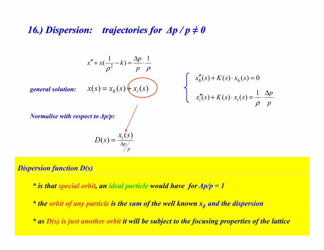
16.) Dispersion: trajectories for 16.) Dispersion: trajectories for ΔΔp / p ≠ 0 p / p ≠ 0

21 1( ) px x k

p ρρΔ′′ + − = ⋅

( ) ( ) ( ) 0x s K s x s′′ + =general solution: ( ) ( ) ( )h ix s x s x s= +

( ) ( ) ( ) 0h hx s K s x s+ ⋅ =

1( ) ( ) ( )i ipx s K s x spρ

Δ′′ + ⋅ = ⋅

Normalise with respect to Δp/p:

( )( ) ix sD s =( ) pp

D s Δ=

Dispersion function D(s)

* is that special orbit, an ideal particle would have for Δp/p = 1

* the orbit of any particle is the sum of the well known x and the dispersion the orbit of any particle is the sum of the well known xβ and the dispersion

* as D(s) is just another orbit it will be subject to the focusing properties of the lattice

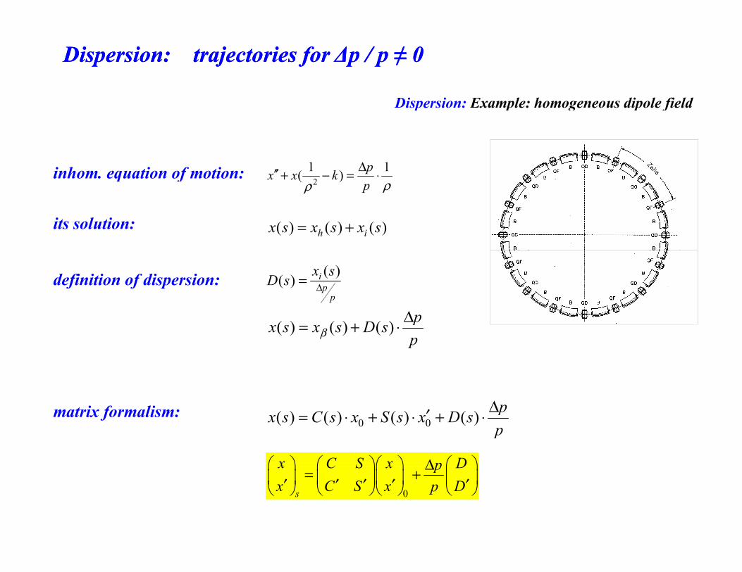
Dispersion: Example: homogeneous dipole field

Dispersion: trajectories for Dispersion: trajectories for ΔΔp / p ≠ 0 p / p ≠ 0

xβ

Dispersion: Example: homogeneous dipole field

xβ1 1( ) px x k Δ′′ + − = ⋅inhom. equation of motion:

.ρ

2( )x x kp ρρ

+

( ) ( ) ( )h ix s x s x s= +

inhom. equation of motion:

its solution:

( ) ( ) ( ) pD Δ

( )( ) ip

p

x sD s Δ=definition of dispersion:

( ) ( ) ( ) px s x s D spβ= + ⋅

matrix formalism:0 0( ) ( ) ( ) ( ) px s C s x S s x D s

pΔ′= ⋅ + ⋅ + ⋅

x C S x Dp⎛ ⎞ ⎛ ⎞⎛ ⎞ ⎛ ⎞Δ

0s

x C S x Dpx C S x Dp

⎛ ⎞ ⎛ ⎞⎛ ⎞ ⎛ ⎞Δ= +⎜ ⎟ ⎜ ⎟⎜ ⎟ ⎜ ⎟′ ′ ′ ′ ′⎝ ⎠ ⎝ ⎠⎝ ⎠ ⎝ ⎠

C S D⎛ ⎞ ⎛ ⎞⎛ ⎞

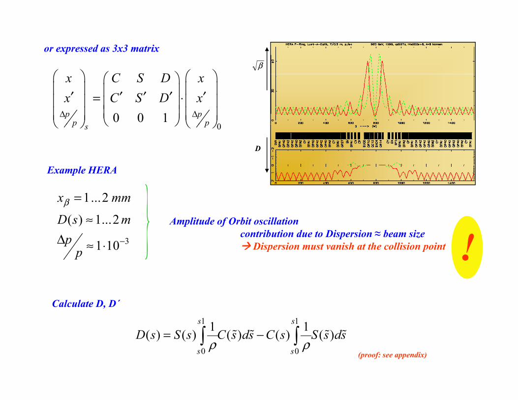
or expressed as 3x3 matrixβ

00 0 1p p

p p

x C S D xx C S D x

Δ Δ

⎛ ⎞ ⎛ ⎞⎛ ⎞⎜ ⎟ ⎜ ⎟⎜ ⎟′ ′ ′ ′ ′= ⋅⎜ ⎟ ⎜ ⎟⎜ ⎟

⎜ ⎟⎜ ⎟ ⎜ ⎟⎝ ⎠⎝ ⎠ ⎝ ⎠0p ps ⎝ ⎠⎝ ⎠ ⎝ ⎠

Example HERA

D

p

1...2

( ) 1...2

x mm

D s mβ =

≈ Amplitude of Orbit oscillation

3

( )

1 10pp

−Δ ≈ ⋅

p fcontribution due to Dispersion ≈ beam size

Dispersion must vanish at the collision point !Calculate D, D´

1 11 1s s

∫ ∫0 0

1 1( ) ( ) ( ) ( ) ( )s s

D s S s C s ds C s S s dsρ ρ

= −∫ ∫% % % %

(proof: see appendix)

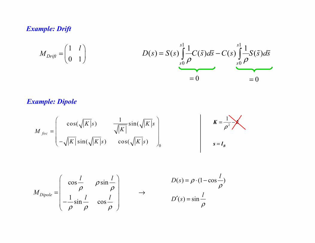
Example: Drift

⎛ ⎞ 1 1s s10 1Drift

lM

⎛ ⎞= ⎜ ⎟⎝ ⎠

1 1

0 0

1 1( ) ( ) ( ) ( ) ( )s s

s s

D s S s C s ds C s S s dsρ ρ

= −∫ ∫% % % %

0= 0=

Example: Dipole

1cos( ) sin(⎛ ⎞⎜ ⎟

= ⎜ ⎟⎜ ⎟⎜ ⎟

foc

K s K sKM

kK −= 2

1ρ

0sin( ) cos( )

⎜ ⎟⎜ ⎟−⎝ ⎠K K s K sBls =

cos sin

1Dipole

l l

Ml l

ρρ ρ

⎛ ⎞⎜ ⎟⎜ ⎟= →⎜ ⎟

( ) (1 cos )

( ) sin

lD s

lD s

ρρ

= ⋅ −

′1 sin cosl lρ ρ ρ

⎜ ⎟−⎜ ⎟⎝ ⎠

( ) sinD sρ

=

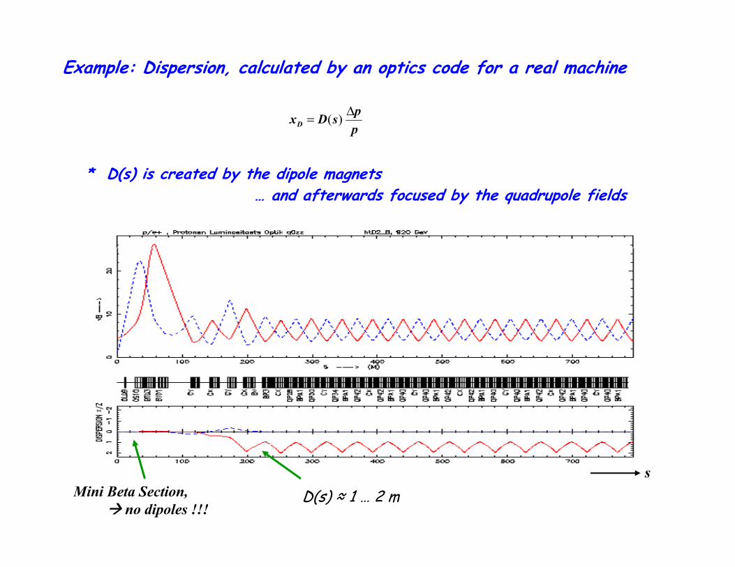
Example: Dispersion, calculated by an optics code for a real machine

ppsDxD

Δ= )(

* D(s) is created by the dipole magnets D(s) is created by the dipole magnets … and afterwards focused by the quadrupole fields

D(s) ≈ 1 … 2 ms

Mini Beta Section, no dipoles !!!

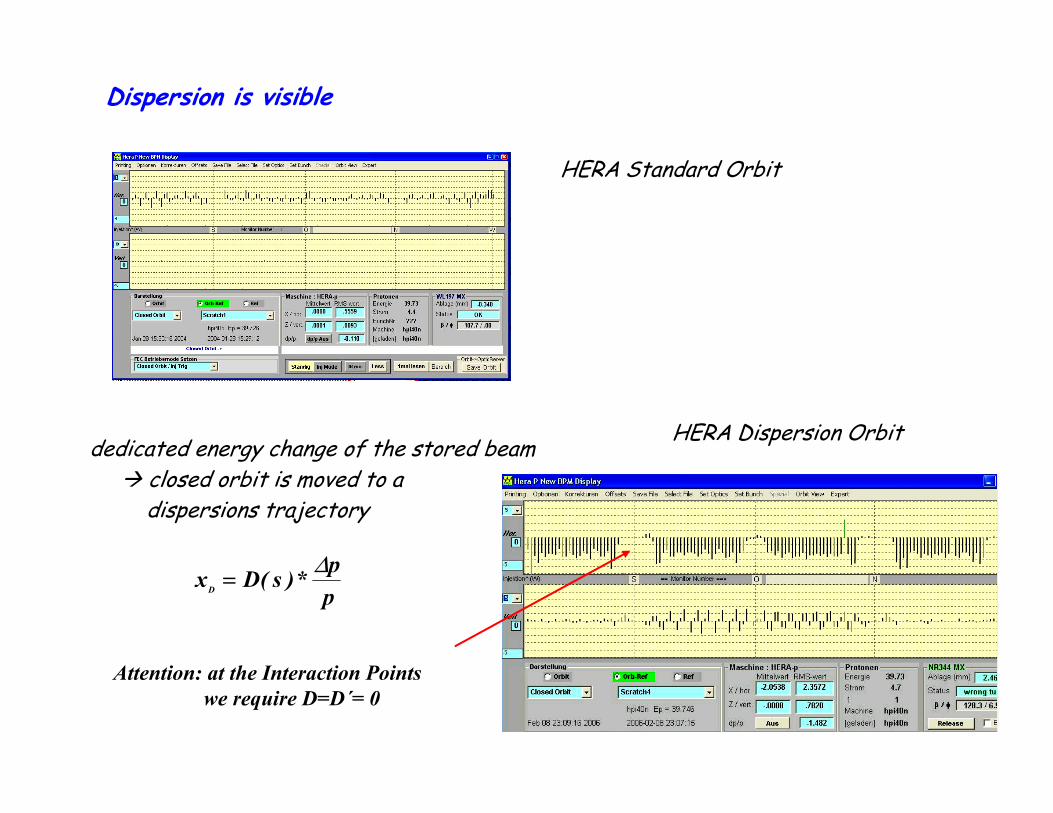
Dispersion is visible

HERA Standard Orbit

dedicated energy change of the stored beamHERA Dispersion Orbit

Δ

gy gclosed orbit is moved to a dispersions trajectory

pp*)s(DxD

Δ=

Attention: at the Interaction Points we require D=D´= 0

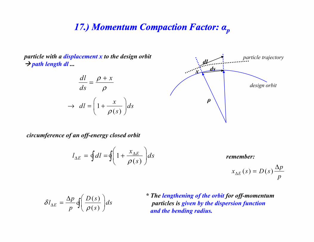
17.) Momentum Compaction Factor: 17.) Momentum Compaction Factor: ααpp

dsxdl

particle trajectoryparticle with a displacement x to the design orbitpath length dl ...

dl

ρ

design orbit

1 xdl ds⎛ ⎞

→ = +⎜ ⎟

dl xds

ρρ+=

1( )

dl dssρ

→ = +⎜ ⎟⎝ ⎠

circumference of an off-energy closed orbit

1( )

EE

xl dl dssρ

ΔΔ

⎛ ⎞= = +⎜ ⎟

⎝ ⎠∫ ∫

circumference of an off energy closed orbit

remember:

pΔ

o o

( ) ( )Epx s D s

pΔΔ=

( )D⎛ ⎞Δ * The lengthening of the orbit for off-momentum( )( )E

p D sl dsp s

δρΔ

⎛ ⎞Δ= ⎜ ⎟⎝ ⎠∫

The lengthening of the orbit for off momentum particles is given by the dispersion function

and the bending radius.o

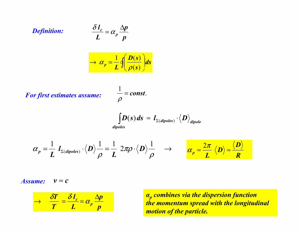
Definition:pp

Ll

pΔ= αδ ε

dsssD

Lp ∫ ⎟⎟⎠

⎞⎜⎜⎝

⎛=→

)()(1

ρα

For first estimates assume: .1 const=ρρ

dipoledipolesdipoles

DldssD ⋅≈ Σ∫ )()(

→⋅=⋅= Σ ρπρ

ρα 12111

)( DL

DlL dipolesp

RD

DLp ≈≈ πα 2

Assume: cv ≈

αp combines via the dispersion function the momentum spread with the longitudinalmotion of the particle.p

pLl

TT

pΔ==→ αδδ ε

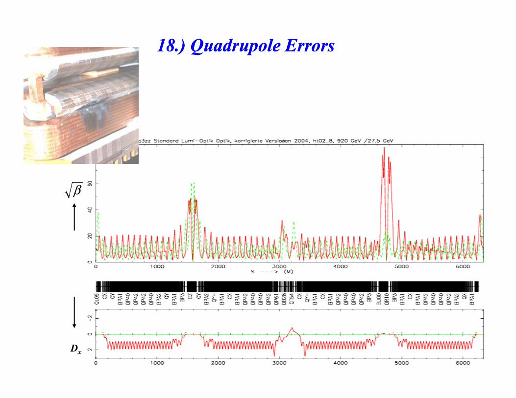
18.) Quadrupole Errors 18.) Quadrupole Errors

β

Dx

⎞⎛⎞⎛ xxgo back to Lecture I page 1

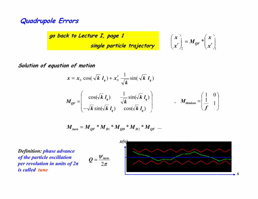
Quadrupole Errors

12

* ⎟⎟⎠

⎞⎜⎜⎝

⎛′

=⎟⎟⎠

⎞⎜⎜⎝

⎛′ x

xM

xx

QF

go back to Lecture I, page 1

single particle trajectory

Solution of equation of motion

)sin(1)cos( 00 qq lkk

xlkxx ′+=

⎟⎟⎟

⎠

⎞

⎜⎜⎜

⎝

⎛

−=

)cos()sin(

)sin(1)cos(

qq

qqQF

lklkk

lkk

lkM ⎟

⎟

⎠

⎞

⎜⎜

⎝

⎛= 11

01,

fM lensthin

⎠⎝

...**** 21 QFDQDDQFturn MMMMMM =

Definition: phase advance of the particle oscillation

l ti i it f 2

x(s)

ψ2

turnQ =per revolution in units of 2πis called tune

s

π2Q

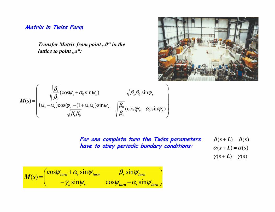
Matrix in Twiss Form

Transfer Matrix from point „0“ in the lattice to point „s“:

⎟⎞

⎜⎛

+ sin)sin(coss ψββψαψβ

( )⎟⎟⎟⎟⎟

⎠⎜⎜⎜⎜⎜

⎝−+−−

+=

)sin(cos(sin)1(cos(

sin)sin(cos)(

00

0

00

000

ssss

ssss

ssss

sMψαψ

ββ

ββψααψαα

ψββψαψβ

For one complete turn the Twiss parameters have to obey periodic bundary conditions: )()(

)()(L

sLs ββ =+have to obey periodic bundary conditions:

)()()()(

sLssLs

γγαα

=+=+

⎟⎞

⎜⎛ + ψβψαψ sinsincos

⎟⎟⎠

⎞⎜⎜⎝

⎛−−

+=

turnsturnss

turnsturnsturnsMψαψψγ

ψβψαψsincossin

sinsincos)(

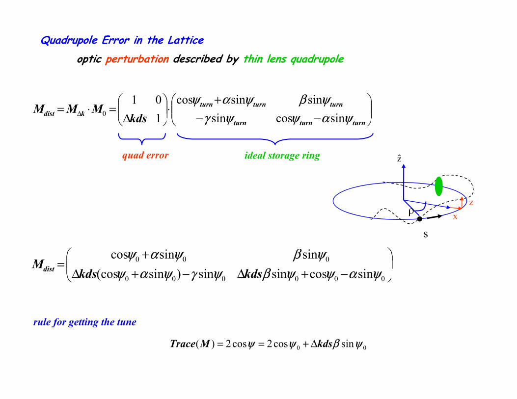
Quadrupole Error in the Latticeoptic perturbation described by thin lens quadrupole

⎟⎟⎠

⎞⎜⎜⎝

⎛−−

+⋅⎟⎟⎠

⎞⎜⎜⎝

⎛Δ

=⋅= Δturnturnturn

turnturnturnkdist kds

MMMψαψψγ

ψβψαψsincossin

sinsincos101

0

ideal storage ringquad error z

⎠⎝⎠⎝ turnturnturn ψψψγ

zρ● x

s

⎟⎟⎠

⎞⎜⎜⎝

⎛−+Δ−+Δ

+= 000

sincossinsin)sin(cossinsincos

ψαψψβψγψαψψβψαψ

kdskdsMdist

rule for getting the tune

⎠⎝ +Δ+Δ 000000 sincossinsin)sin(cos ψαψψβψγψαψ kdskds

f g g

00 sincos2cos2)( ψβψψ kdsMTrace Δ+==

sincos)cos( 0ψβψψψ kdsΔ+=Δ+

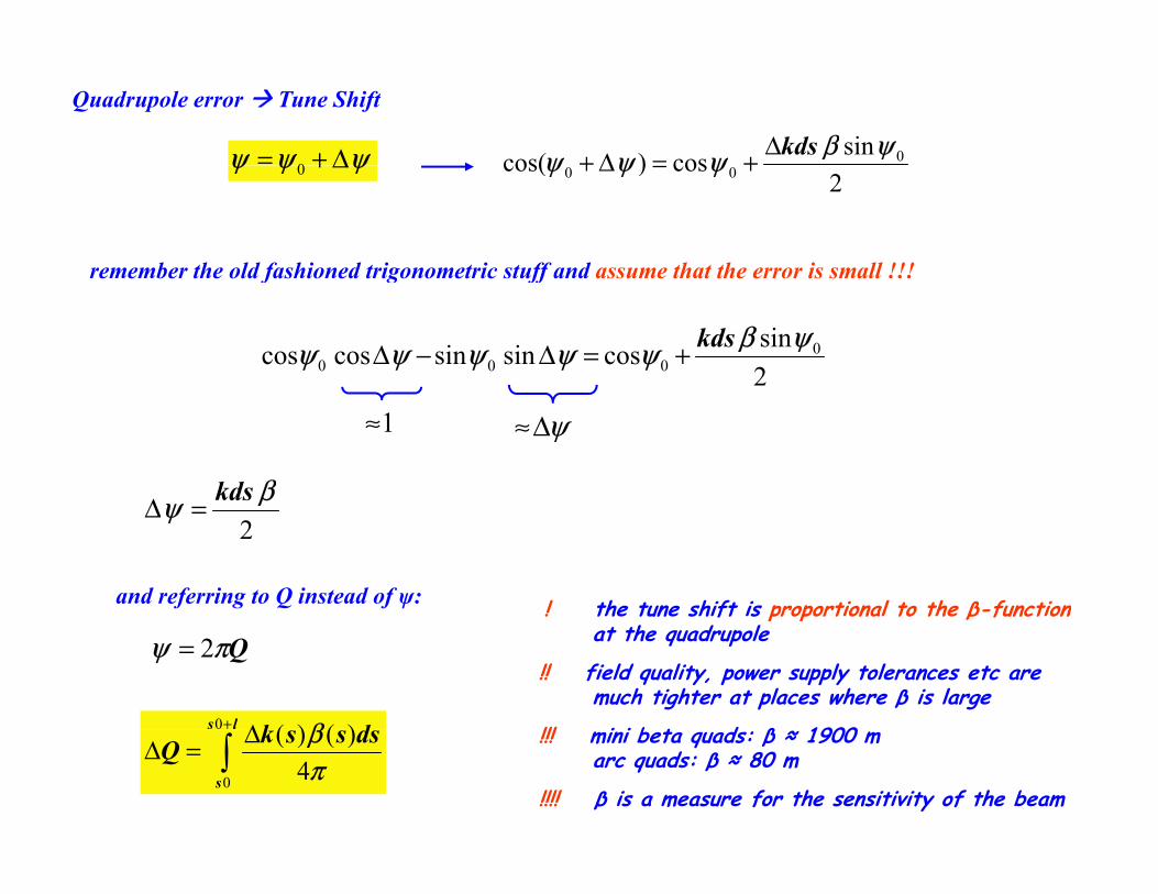
Quadrupole error Tune Shift

ψψψ Δ+= 0

remember the old fashioned trigonometric stuff and assume that the error is small !!!

2cos)cos( 00 ψψψ +=Δ+ψψψ Δ+0

remember the old fashioned trigonometric stuff and assume that the error is small !!!

2sincossinsincoscos 0

000ψβψψψψψ kds+=Δ−Δ

1≈ ψ≈Δ

βψ kdsΔ

and referring to Q instead of ψ: ! the tune shift is proportional to the β-function

2βψ =Δ

Qπψ 2=

+ Δls dk0 )()( β

! the tune sh ft s proport ona to the β funct onat the quadrupole

!! field quality, power supply tolerances etc are much tighter at places where β is large

!!! i i b t d β 1900∫

Δ=Δs

dssskQ0 4

)()(πβ !!! mini beta quads: β ≈ 1900 m

arc quads: β ≈ 80 m

!!!! β is a measure for the sensitivity of the beam

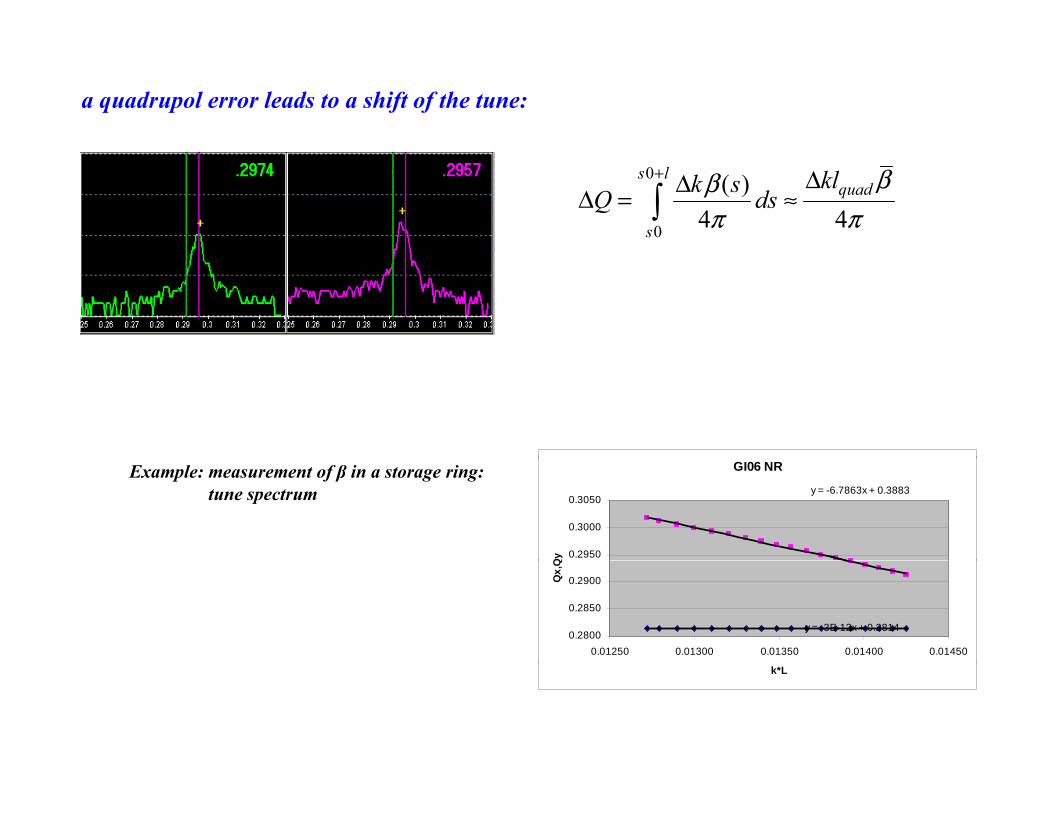
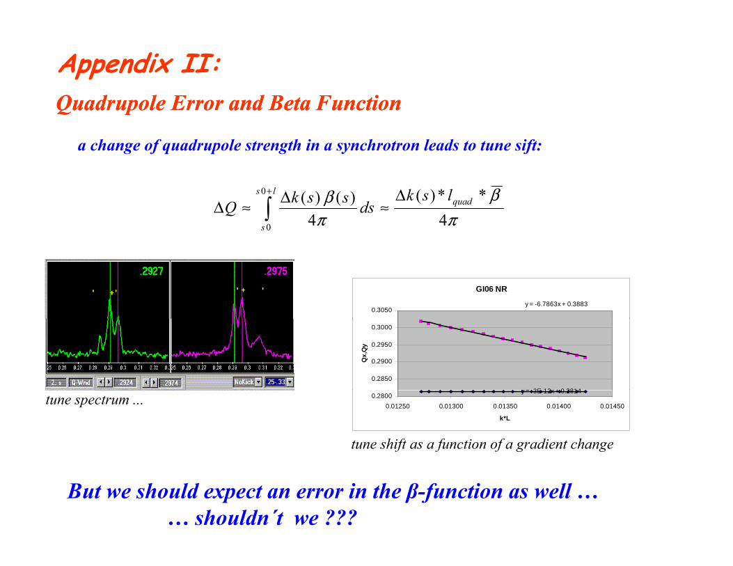
a quadrupol error leads to a shift of the tune:

0

0

( )4 4

s lquad

s

klk sQ dsββ

π π

+ ΔΔΔ = ≈∫

Example: measurement of β in a storage ring:tune spectrum

GI06 NR

y = -6.7863x + 0.3883

0.2950

0.3000

0.3050

Qy

y = -3E-12x + 0.28140.2800

0.2850

0.2900

0.01250 0.01300 0.01350 0.01400 0.01450

Qx,

Q

k*L

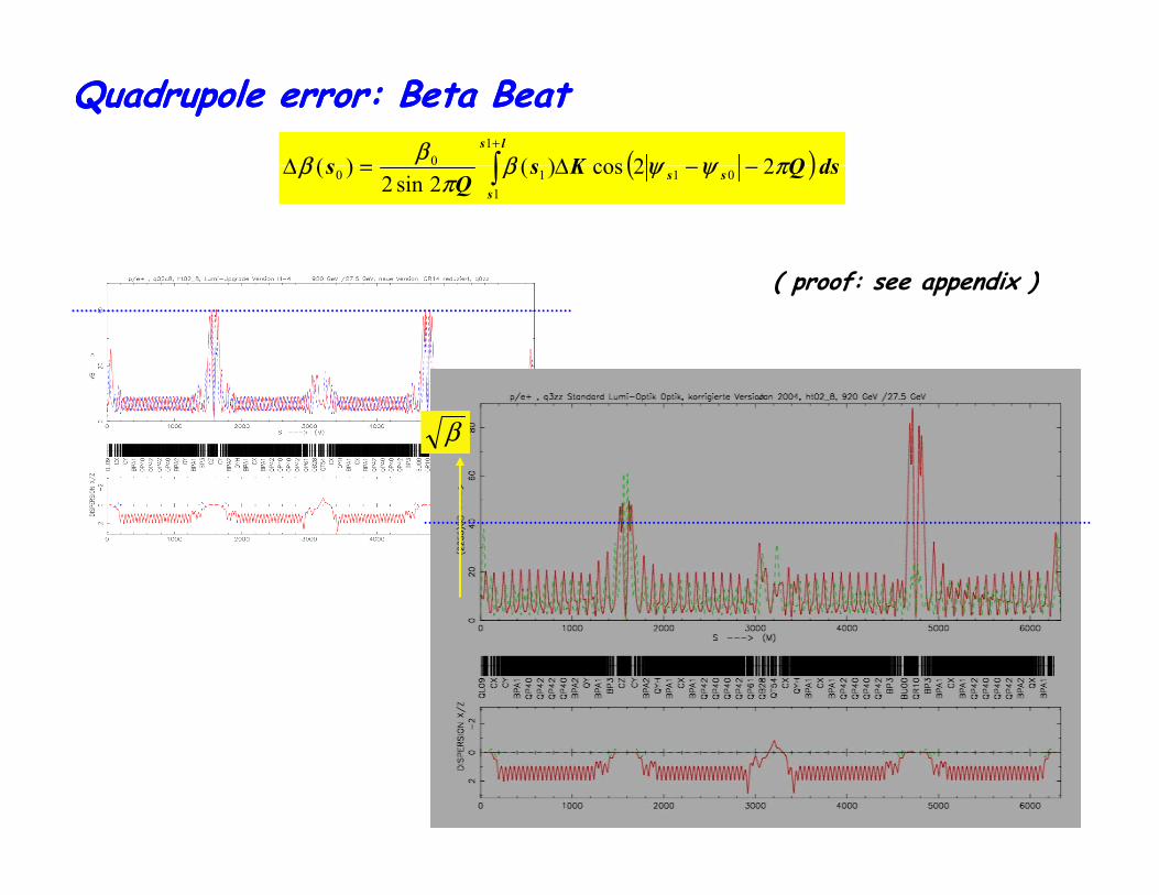
Quadrupole error: Quadrupole error: Beta Beat Beta Beat

( )dsQKssls

πψψβββ 22cos)()(1

0 Δ=Δ ∫+

( proof: see appendix )

( )dsQKsQ

s sss

πψψβπ

β 22cos)(2sin2

)( 011

10 −−Δ=Δ ∫

( proof: see appendix )

β

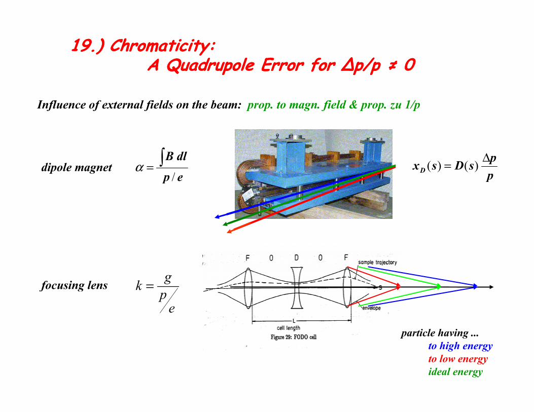
19.) Chromaticity: 19.) Chromaticity: A Quadrupole Error for A Quadrupole Error for ∆∆p/p p/p ≠≠ 00

Influence of external fields on the beam: prop. to magn. field & prop. zu 1/p

dipole magnetep

dlB

/∫=α

ppsDsxD

Δ= )()(ep / p

focusing lens gkfocusing lens gk pe

=

particle having ...particle having ... to high energyto low energyideal energy

gk =

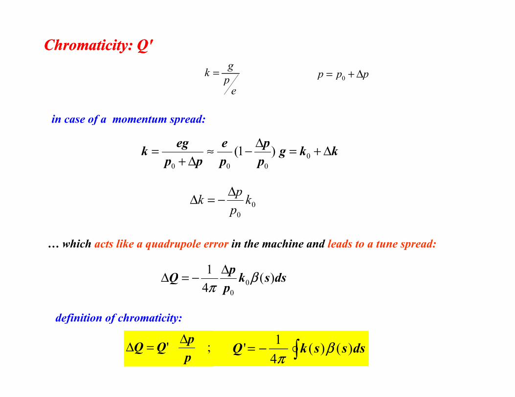
Chromaticity: Chromaticity: Q'Q'

p p p= + Δk pe

=

in case of a momentum spread:

0p p p= + Δ

f p

kkgpp

pe

ppegk Δ+=Δ−≈

Δ+= 0

000

)1(

00

kppk Δ−=Δ

… which acts like a quadrupole error in the machine and leads to a tune spread:

dkpQ )(1 βΔΔ

definition of chromaticity:

dsskppQ )(

4 00

βπ

−=Δ

f f y

∫−= dssskQ )()(41' βπ

;'ppQQ Δ=Δ

Where is the Problem ?

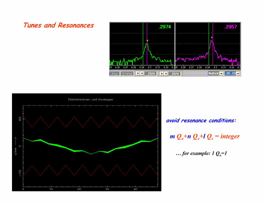
Tunes and Resonances

avoid resonance conditions:

m Qx+n Qy+l Qs = integer

… for example: 1 Qx=1

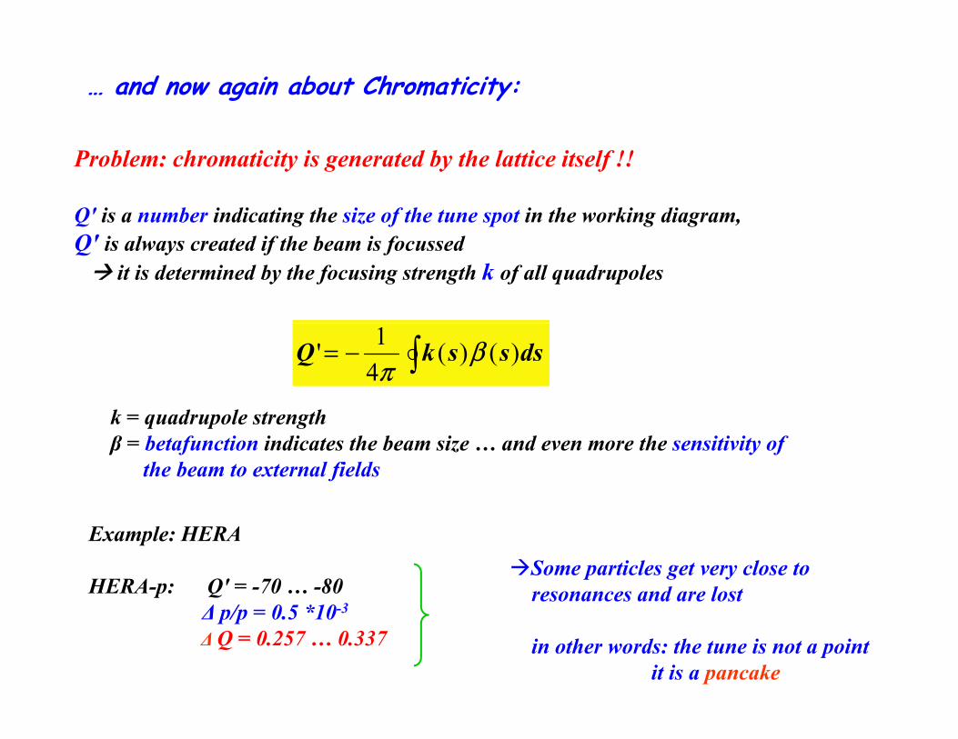
… and now again about Chromaticity:

Problem: chromaticity is generated by the lattice itself !!

Q' is a number indicating the size of the tune spot in the working diagram, Q' is always created if the beam is focussed

it is determined by the focusing strength k of all quadrupoles

k = quadrupole strength

∫−= dssskQ )()(41' βπ

k = quadrupole strengthβ = betafunction indicates the beam size … and even more the sensitivity of

the beam to external fields

Example: HERA

HERA-p: Q' = -70 … -80 Some particles get very close to resonances and are lost

Δ p/p = 0.5 *10-3

ΔQ = 0.257 … 0.337 in other words: the tune is not a pointit is a pancake

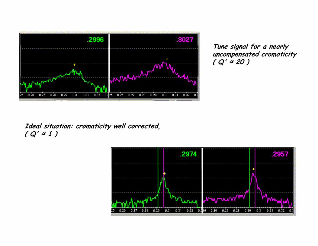
Tune signal for a nearlyTune signal for a nearly uncompensated cromaticity( Q' ≈ 20 )

Ideal situation: cromaticity well corrected,( Q' ≈ 1 )

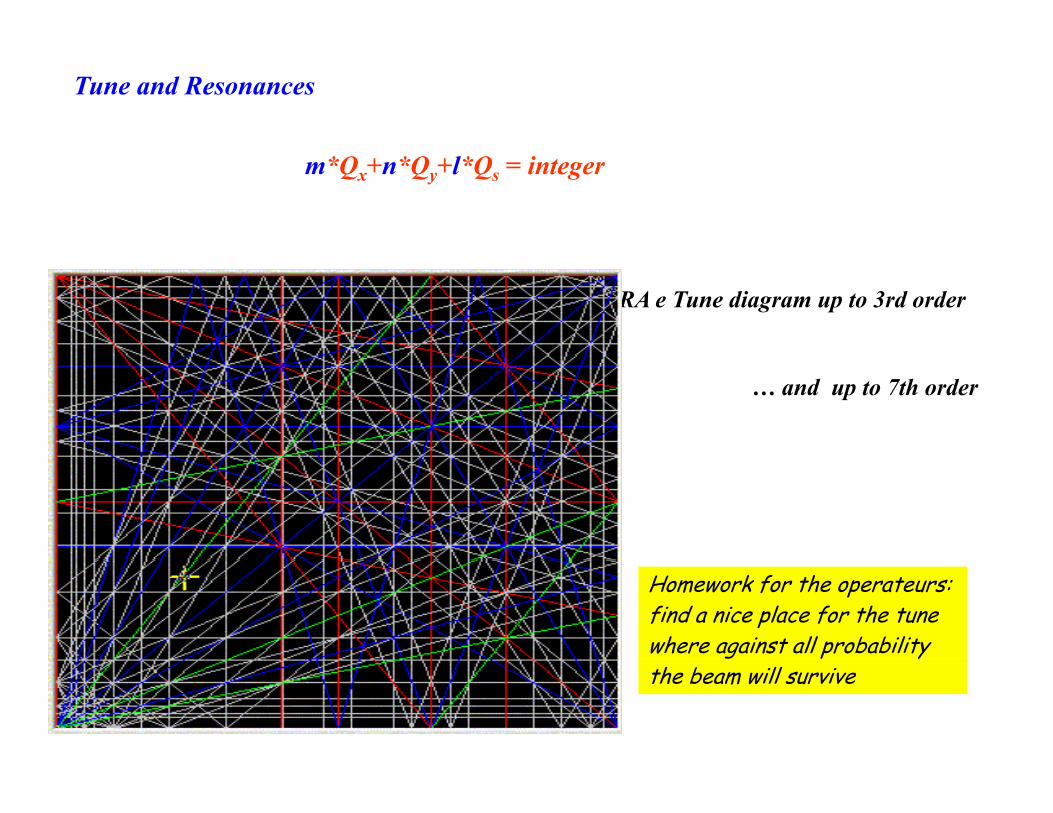
Tune and Resonances

m*Qx+n*Qy+l*Qs = integer

Qy =1.5 HERA e Tune diagram up to 3rd order

Qy =1.3… and up to 7th order

Qy =1.0

Homework for the operateurs: find a nice place for the tune where against all probability

Qx =1.0 Qx =1.3

Qy 1.0

Qx =1.5the beam will survive

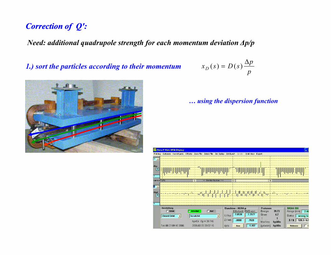
Correction of Correction of Q'Q': :

Need: additional quadrupole strength for each momentum deviation Δp/p

1.) sort the particles according to their momentum ( ) ( )Dpx s D s

pΔ=

… using the dispersion function

Correction of Q':Correction of Q':

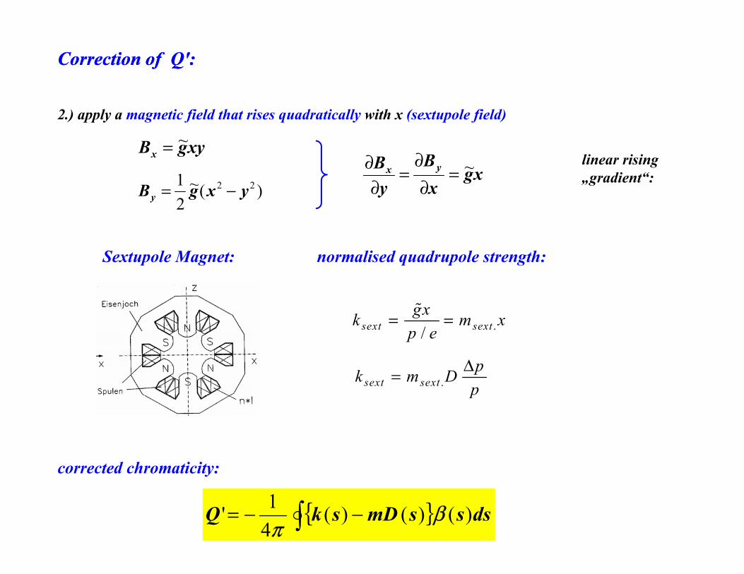
2.) apply a magnetic field that rises quadratically with x (sextupole field)

linear rising gradient“:

xygBx~=

1 xgBB yx ~=

∂=∂

S l M

„gradient :

li d d l h

)(~21 22 yxgBy −=

xgxy ∂∂

Sextupole Magnet: normalised quadrupole strength:

t tgxk m x= =%

./sext sextk m xp e

.sext sextpk m D

pΔ=

corrected chromaticity:

p

corrected chromaticity:

{ }∫ −−= dsssmDskQ )()()(41' βπ

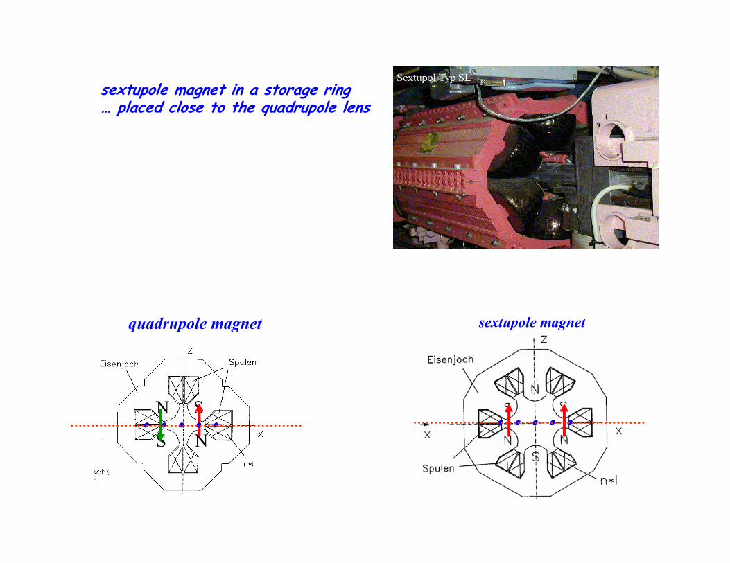
sextupole magnet in a storage ringl d l t th d l l… placed close to the quadrupole lens

lquadrupole magnet sextupole magnet

S

S

N

N● ● ● ● ●● ● ● ● ●

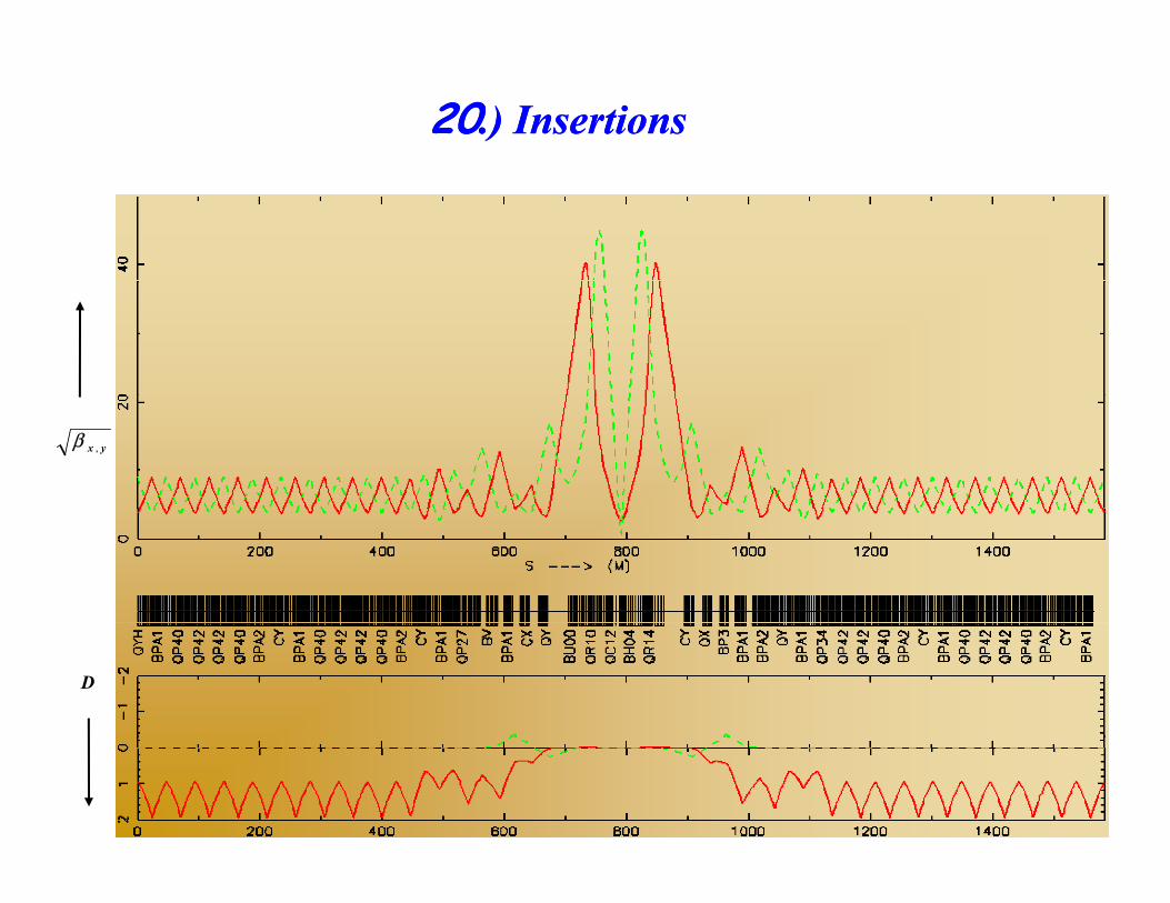
2020.) Insertions.) Insertions

yx ,β

D

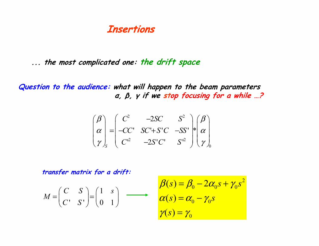
InsertionsInsertions

... the most complicated one: the drift space

Question to the audience: what will happen to the beam parameters α, β, γ if we sstop focusing for a while …?

2 2

2 2

2' ' ' ' *

C SC SCC SC S C SS

β βα α

⎛ ⎞−⎛ ⎞ ⎛ ⎞⎜ ⎟⎜ ⎟ ⎜ ⎟= − + −⎜ ⎟⎜ ⎟ ⎜ ⎟

⎜ ⎟ ⎜ ⎟⎜ ⎟2 20

' 2 ' ' 'S

C S C Sγ γ⎜ ⎟ ⎜ ⎟⎜ ⎟−⎝ ⎠ ⎝ ⎠⎝ ⎠

f i f d iftransfer matrix for a drift:

1' ' 0 1

C S sM

C S⎛ ⎞ ⎛ ⎞

= =⎜ ⎟ ⎜ ⎟⎝ ⎠ ⎝ ⎠

20 0 0

0 0

( ) 2( )s s ss s

β β α γα α γ

= − += −' ' 0 1C S⎜ ⎟ ⎜ ⎟

⎝ ⎠ ⎝ ⎠ 0 0

0

( )( )s ss

α α γγ γ=

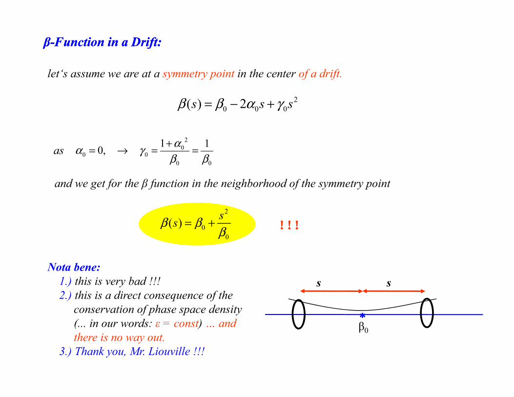
ββ--Function in a Drift:Function in a Drift:

let‘s assume we are at a symmetry point in the center of a driftlet s assume we are at a symmetry point in the center of a drift.

20 0 0( ) 2s s sβ β α γ= − +

as20

0 00 0

1 10, αα γβ β

+= → = =

and we get for the β function in the neighborhood of the symmetry point

! ! !! ! !2

( ) ssβ β= +

Nota bene:

! ! !! ! !00

( )sβ ββ

= +

1.) this is very bad !!!2.) this is a direct consequence of the

conservation of phase space density( in our words: ε = const) and **

s s

β(... in our words: ε = const) … and there is no way out.

3.) Thank you, Mr. Liouville !!!

β0

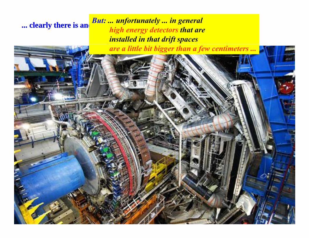
... clearly there is another problem !!!... clearly there is another problem !!!

Example: Luminosity optics at LHC: β* = 55 cm

But: ... unfortunately ... in general high energy detectors that are installed in that drift spaces p y p β

for smallest βmax we have to limit the overall length and keep the distance “s” as small as possible.

are a little bit bigger than a few centimeters ...

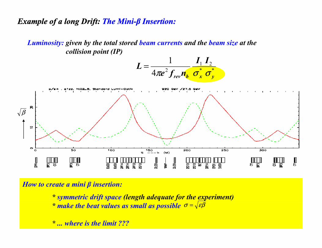
Example of a long Drift:Example of a long Drift: The MiniThe Mini--ββ Insertion:Insertion:

Luminosity: given by the total stored beam currents and the beam size at the y g ycollision point (IP)

**21

241

yxbrev

IInfe

Lσσπ

=yxbrevf

β

How to create a mini β insertion:

* symmetric drift space (length adequate for the experiment)β* make the beat values as small as possible

* ... where is the limit ???

εβσ =

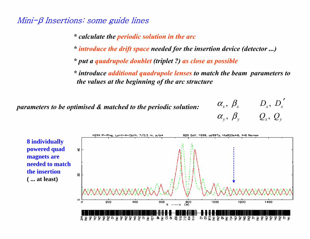
Mini-β Insertions: some guide lines

* calculate the periodic solution in the arc

* introduce the drift space needed for the insertion device (detector ...)

* put a quadrupole doublet (triplet ?) as close as possible

* introduce additional quadrupole lenses to match the beam parameters to introduce additional quadrupole lenses to match the beam parameters to the values at the beginning of the arc structure

b i i d & h d h i di l i D Dα β ′parameters to be optimised & matched to the periodic solution: , ,

, ,x x x x

y y x y

D DQ Q

α βα β

8 individually powered quad magnets are needed to matchneeded to match the insertion ( ... at least)

∫−= dssskQ )()(41' β

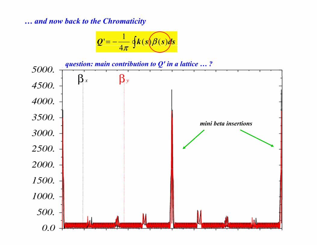
… and now back to the Chromaticity

∫Q )()(4

βπ

question: main contribution to Q' in a lattice … ?

mini beta insertions

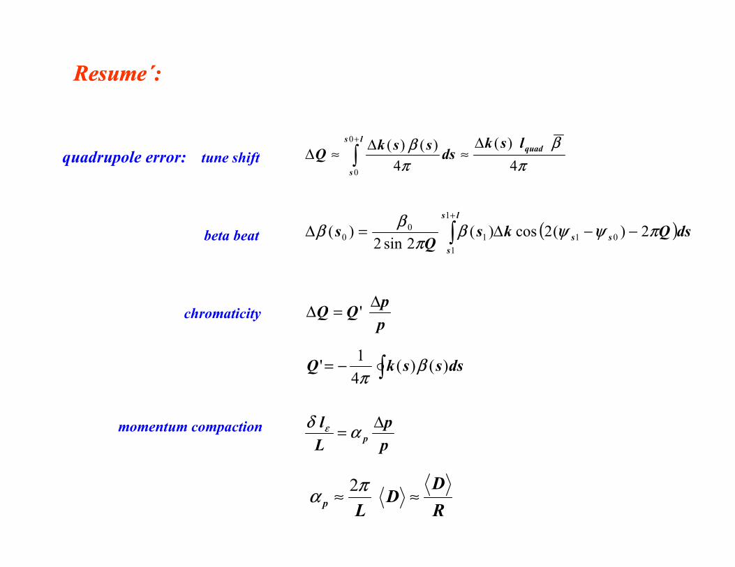
ResumeResume´::

quadrupole error: tune shift πβ

πβ

4)(

4)()(0

0

quadls

s

lskdssskQ

Δ≈Δ≈Δ ∫

+

beta beat ( )dsQksQ

s ss

ls

πψψβπ

ββ 2)(2cos)(2sin2

)( 01

1

11

00 −−Δ=Δ ∫

+

chromaticity

Q sπ2sin2 1

pQQ Δ=Δ 'y

∫−= dssskQ )()(41' βπ

pQQ

momentum compaction pp

Ll

pΔ= αδ ε

RD

DLp ≈≈ πα 2

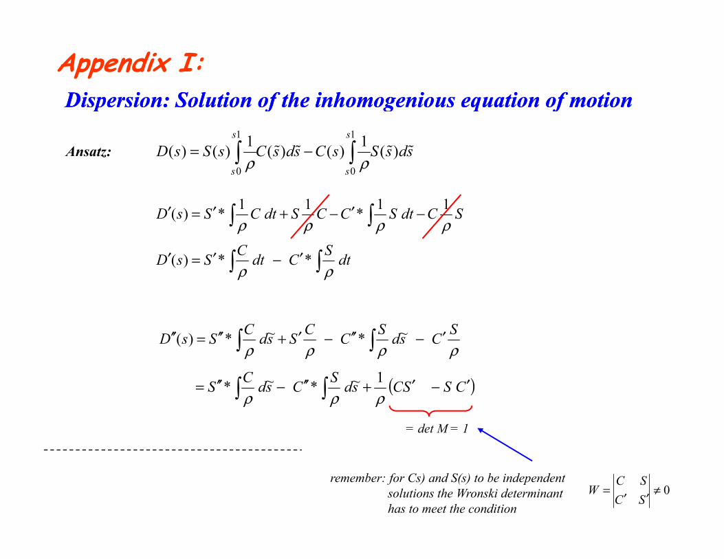
Dispersion: Solution of the inhomogenious equation of motionDispersion: Solution of the inhomogenious equation of motionAppendix I:Dispersion: Solution of the inhomogenious equation of motionDispersion: Solution of the inhomogenious equation of motion

1 1

0 0

1 1( ) ( ) ( ) ( ) ( )s s

s s

D s S s C s ds C s S s dsρ ρ

= −∫ ∫% % % %Ansatz:0 0s s

SCdtSCCSdtCSsDρρρρ11*11*)( −′−+′=′ ∫∫

∫∫ ′−′=′ dtSCdtCSsDρρ

**)(

ρρρρSCsdSCCSsdCSsD ′−′′−′+′′=′′ ∫∫ ~*~*)(

( )CSSCsdSCsdCS ′′+′′′′ ∫∫1~*~* ( )CSSCsdCsdS −+−= ∫∫ ρρρ

**

= det M = 1

remember: for Cs) and S(s) to be independentsolutions the Wronski determinant has to meet the condition

0≠′′

=SCSC

W

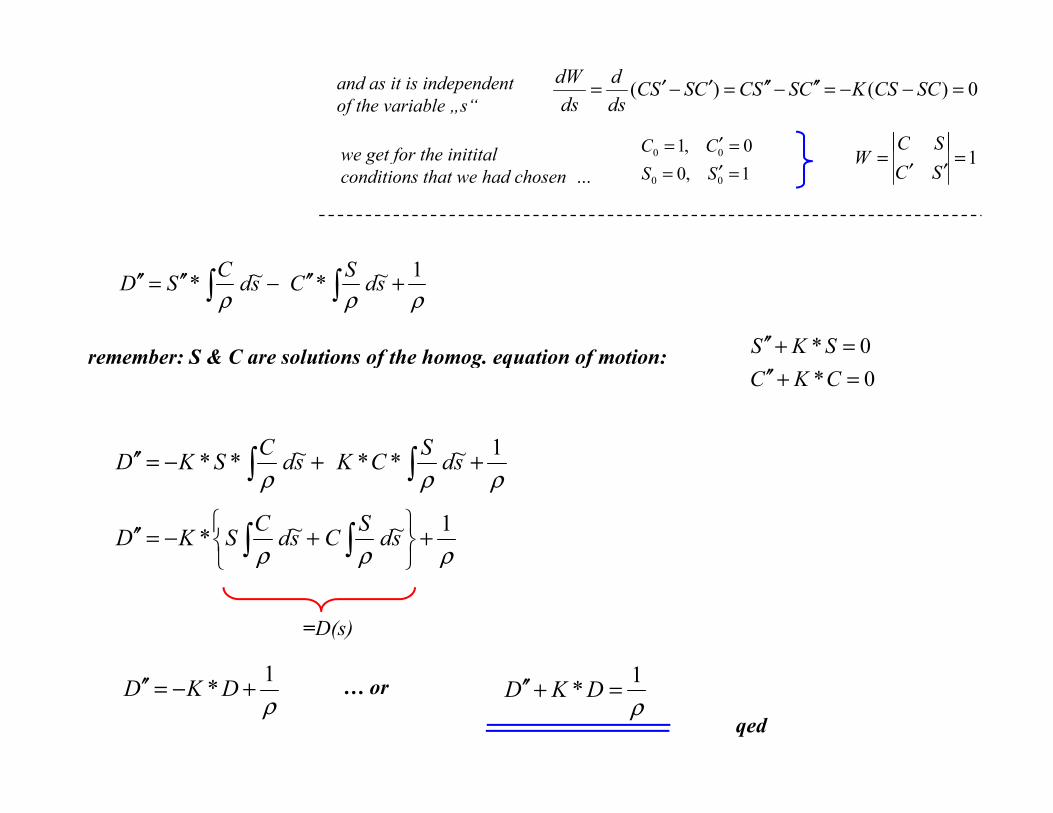
and as it is independent of the variable „s“

0)()( =−−=′′−′′=′−′= SCCSKCSSCCSSCdsd

dsdW

t f th i itit l 0,1 00 =′= CC SCwe get for the initital conditions that we had chosen … 1,0

0,1

00

00

=′= SSCC 1=

′′=

SCW

remember: S & C are solutions of the homog equation of motion: 0* =+′′ SKS

ρρρ1~*~* +′′−′′=′′ ∫∫ sdSCsdCSD

remember: S & C are solutions of the homog. equation of motion:0* =+′′ CKC

1~**~** ++′′ ∫∫ dSCKdCSKDρρρ

**** ++−= ∫∫ sdCKsdSKD

ρρρ1~~* +

⎭⎬⎫

⎩⎨⎧ +−=′′ ∫∫ sdSCsdCSKD

ρρρ ⎭⎩

=D(s)

ρ1* +−=′′ DKD … or

ρ1* =+′′ DKD

qed

Quadrupole Error and Beta FunctionQuadrupole Error and Beta Function

Appendix II:

a change of quadrupole strength in a synchrotron leads to tune sift:

Quadrupole Error and Beta FunctionQuadrupole Error and Beta Function

πβ

πβ

4**)(

4)()(0

0

quadls

s

lskdssskQ

Δ≈Δ≈Δ ∫

+

GI06 NR

y = -6.7863x + 0.38830.3050

y = 3E 12x + 0 2814

0.2850

0.2900

0.2950

0.3000

Qx,

Qy

y = -3E-12x + 0.28140.2800

0.01250 0.01300 0.01350 0.01400 0.01450

k*L

tune spectrum ...

tune shift as a function of a gradient change

But we should expect an error in the β-function as well …… shouldn´t we ???

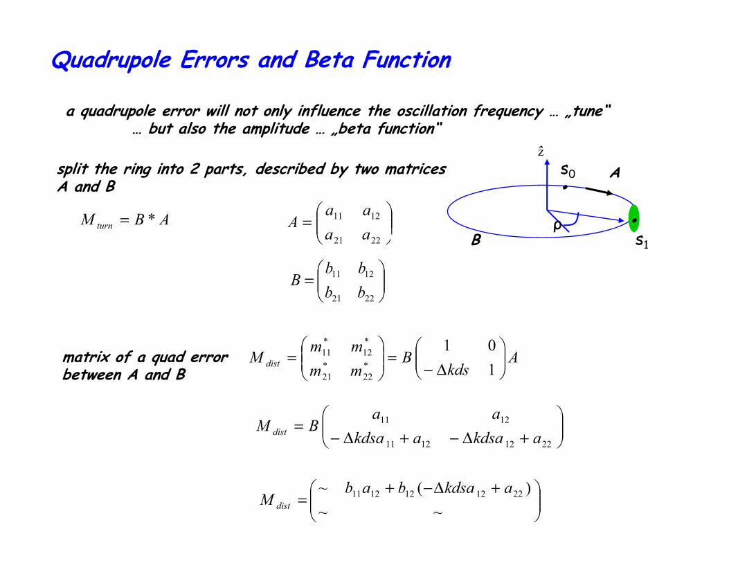
Quadrupole Errors and Beta Function

l ll l l ll “

split the ring into 2 parts, described by two matrices

a quadrupole error will not only influence the oscillation frequency … „tune“ … but also the amplitude … „beta function“

s0

z

Ap g p , yA and B

ABM turn *= ⎟⎟⎠

⎞⎜⎜⎝

⎛=

2221

1211

aaaa

A ρ

0●

s1

●

A

B

⎟⎟⎠

⎞⎜⎜⎝

⎛=

2221

1211

bbbb

B

1

matrix of a quad error between A and B

Akds

Bmmmm

M dist ⎟⎟⎠

⎞⎜⎜⎝

⎛Δ−

=⎟⎟⎠

⎞⎜⎜⎝

⎛=

101

*22

*21

*12

*11

⎟⎟⎠

⎞⎜⎜⎝

⎛+Δ−+Δ−

=22121211

1211

akdsaakdsaaa

BM dist

⎟⎟⎠

⎞⎜⎜⎝

⎛ +Δ−+=

~~)(~ 2212121211 akdsabab

M dist

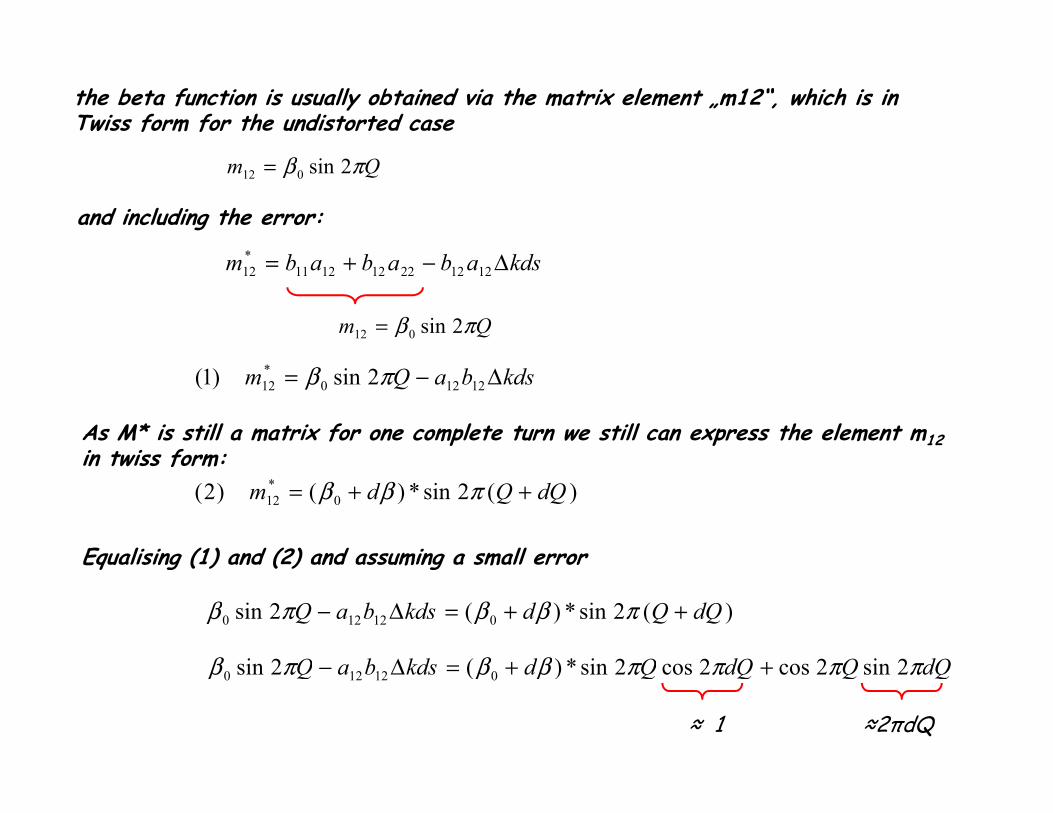
the beta function is usually obtained via the matrix element „m12“, which is in Twiss form for the undistorted case

Qm πβ 2sin012 =

*

and including the error:

kdsabababm Δ−+= 121222121211*12

Qm πβ 2sin012 =

kdsbaQm Δ−= 12120*12 2sin)1( πβ

As M* is still a matrix for one complete turn we still can express the element m12 in twiss form:in twiss form:

)(2sin*)()2( 0*12 dQQdm ++= πββ

Equalising (1) and (2) and assuming a small errorEqualising (1) and (2) and assuming a small error

)(2sin*)(2sin 012120 dQQdkdsbaQ ++=Δ− πββπβ

dQQdQQdkdbQ ππππββπβ 2i222i*)(2i ++Δ dQQdQQdkdsbaQ ππππββπβ 2sin2cos2cos2sin*)(2sin 012120 ++=Δ−

≈ 1 ≈2πdQ

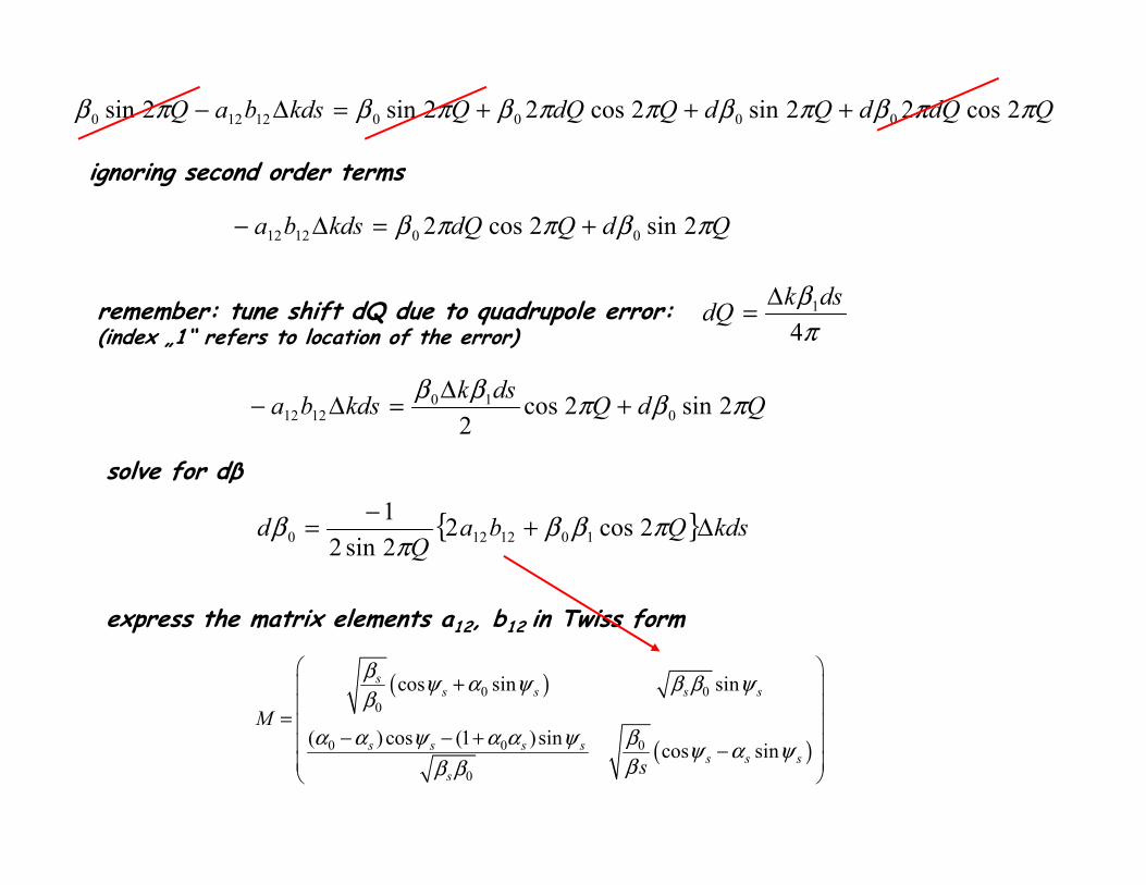
QdQdQdQdQQkdsbaQ ππβπβππβπβπβ 2cos22sin2cos22sin2sin 000012120 +++=Δ−

i i d d

QdQdQkdsba πβππβ 2sin2cos2 001212 +=Δ−

ignoring second order terms

remember: tune shift dQ due to quadrupole error:(index „1“ refers to location of the error) π

β41dskdQ Δ=

dskββ Δ QdQdskkdsba πβπββ 2sin2cos2 0

101212 +Δ=Δ−

solve for dβ

{ } kdsQbaQ

d Δ+−= πββπ

β 2cos22sin21

1012120

h i l b i T i f

( )0 00cos sin sin

⎛ ⎞+⎜ ⎟

⎜ ⎟= ⎜ ⎟

ss s s s

M

β ψ α ψ β β ψβ

express the matrix elements a12, b12 in Twiss form

( )0 0 0

0

( ) cos (1 )sin cos sin= ⎜ ⎟− − +⎜ ⎟−⎜ ⎟⎝ ⎠

s s s ss s s

s

M

sα α ψ α α ψ β ψ α ψ

ββ β

{ } kdsQbaQ

d Δ+−= πββπ

β 2cos22sin21

1012120

)2sin(

sin

100112

101012

→

→

Δ−=

Δ=

ψπββ

ψββ

Qb

a

{ } kdsQQQ

d Δ+Δ−Δ−= πψπψπβββ 2cos)2sin(sin22sin2 1212

100

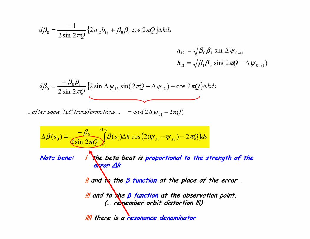
… after some TLC transformations … )22cos( 01 Qπψ −Δ=

( )dQkls

βββ 2)(2)()(1

0 Δ−Δ ∫+

( )dsQksQ

s sss

πψψβπ

ββ 2)(2cos)(2sin2

)( 011

10

0 −−Δ=Δ ∫

Nota bene: ! the beta beat is proportional to the strength of the error ∆kerror ∆k

!! and to the β function at the place of the error ,

!!! and to the β function at the observation point!!! and to the β function at the observation point, (… remember orbit distortion !!!)

!!!! there is a resonance denominator