Ivovi's Lecture 1

8/6/2019 Ivovi's Lecture 1

http://slidepdf.com/reader/full/ivovis-lecture-1 1/45

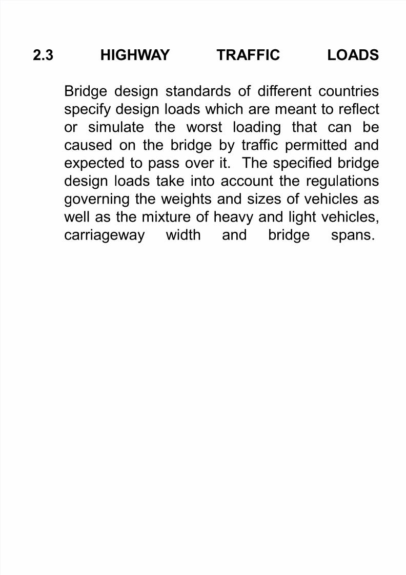
2.3 HIGHWAY TRAFFIC LOADS

Bridge design standards of different countries

specify design loads which are meant to reflect

or simulate the worst loading that can be

caused on the bridge by traffic permitted andexpected to pass over it. The specified bridge

design loads take into account the regulations

governing the weights and sizes of vehicles as

well as the mixture of heavy and light vehicles,carriageway width and bridge spans.



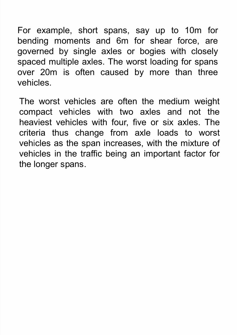
For example, short spans, say up to 10m for

bending moments and 6m for shear force, aregoverned by single axles or bogies with closely

spaced multiple axles. The worst loading for spans

over 20m is often caused by more than three

vehicles.

The worst vehicles are often the medium weight

compact vehicles with two axles and not the

heaviest vehicles with four, five or six axles. Thecriteria thus change from axle loads to worst

vehicles as the span increases, with the mixture of

vehicles in the traffic being an important factor for

the longer spans.



When axles or single vehicles are the worst case,

the effect of impact has to be allowed for, but several

closely spaced vehicles represent a jam situationwithout significant impact. The adjacent lanes of

short span bridges may all be loaded simultaneously

with the worst axles or vehicles, but this is less likely

for long span.

There is the growing problem of illegal overweight

vehicles weighing as much as 40% over their legal

limits to deal with.We shall now see how some of the design codes

specify and apply the primary live loads. We shall

consider examples from the United Kingdom and

the United States of America.



2.3.1 Design Live Loads in the UK

In the United Kingdom, bridge design loading isspecified in the Department of Transport

Standard, BD37/88, which is the composite

version of BS 5400 Part 2: 1978. BD 37/88

incorporates all the amendments that were to be

made to the BS, due to changes observed in the

normal traffic on most British roads, before joining

the EU.

The Standard refers to normal primary traffic

loading as Type HA and abnormal vehicles as

Type HB.



2.3.1.1 HA Loading

HA loading is represented by a theoretical loading

model consisting of a uniformly distributed load

(HAU) combined with a Knife-edge load (HAK) of

120 kN per lane placed across the width of eachnotional lane. (The knife edge load is an attempt to

model the effect of a single localized heavy axle

and is placed on the span where its effect is

maximized for bending and shear). All bridgesshould be designed to resist this loading.



The uniformly distributed lane loading, W per linear

metre of lane, is represented as a curve whoseequation is

W = 336 (1/L)2/3 of lane for loaded

length in the direction of traffic up to 50m

and W = 36 (1/L)1/10 of lane for loaded length in

direction of traffic between 50m and 1600m.

W for L > 1600 m should be agreed

with the appropriate authority.



On loaded lengths of up to 30m, the loading

represents the effects of closely spaced vehicles of 24t laden weight, i.e. trucks. Above this figure, the

intensity gradually decreases to a constant value

for loaded lengths of 380m or more.

This longitudinal attenuation of loads is an attempt

to model the real-life situation where the intensity of

the 24t vehicles is likely to decrease as the loaded

length increases.



The dynamic effect of moving vehicles on a bridge

arises from imperfections in the surfacing, the short

duration of loading, and the vehicles¶ suspension

systems.

No separate calculation is required for impact as

the standard loadings given include a 25% impact

allowance.

It should be noted that the HA loading curves cater

for vehicles up to a gross weight of 40t, provided

that enough axles and wheels are present to

distribute the load so that the effects are the same.



2.3.1.1.1 Primary Single Wheel Load

A single wheel load (HAW) of 100KN can be

placed on small areas of roadway to replace the

effects of HAU and HAK.

The contact area of the wheel on the road surface

is uniformly distributed over a circle of 340mm or

a square of side 300mm giving a contact stress of

1.1N/mm2.



This form of HA loading is used where the

distribution of loads is small and so a member maybe required to take virtually the full weight of a

wheel.

It is frequently applied to the top slabs betweenlongitudinal beams in order to calculate the local

effect of wheel loads.





As such vehicles travel slowly, no impact allowance

is made.

Also, since movement of such vehicles usually

involves a police escort, it is reasonable to assume

that they occupy a single traffic lane alone. (O

nlong bridges the occupied lane is assumed clear for

25m ahead and behind the vehicle, with normal HA

loading occupying the remainder).





2.3.1.4 Secondary Braking Loads

This is considered as a group effect as far as HA

loads are concerned, and assumes that the traffic in

one lane brakes simultaneously over the entire

loaded length. The effect is considered as alongitudinal force applied at the road surface.

There is considerable evidence to suggest that the

force is dissipated to a considerable extent in plan,and for most concrete and composite shallow deck

structures it is reasonable to consider the load

spread over the entire width of the deck.



The braking of an HB vehicle is an isolated effect

distributed evenly between eight wheels of two

axles only of the vehicle and is dissipated as for the

HA load.

The significance of the braking load on the

structure is twofold, namely,



�The design of the bridge abutments or piers whereit is applied as an horizontal load at bearing level,

thus increasing the bending moments in the stem

and footings, and

�The design of the bridge bearings if composed of

an elastomeric bearing resisting horizontal loading

shear.



Traffic Load

HA 8KN /m of loaded length + 250kN ( but � 750KN)

HB Nominal HB load x 0.25

The Code design loads are shown below

Braking Loads



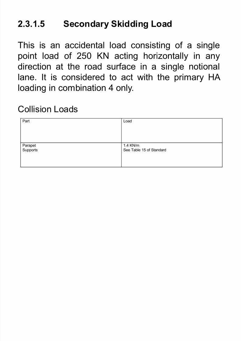
Part Load

ParapetSupports

1.4 KN/mSee Table 15 of Standard

2.3.1.5 Secondary Skidding Load

This is an accidental load consisting of a singlepoint load of 250 KN acting horizontally in any

direction at the road surface in a single notional

lane. It is considered to act with the primary HA

loading in combination 4 only.

Collision Loads



2.3.1.5 Secondary Centrifugal Loads

These loads are important only on elevated

curved superstructures with a radius of less than

1000m supported on slender piers. BD 37/88 givesthe centrifugal load as

Fc=40,000/(r+150)



2.3.1.6 Partial Safety Factors

All loads specified in Standard BD 37/88 arenominal (that is, they are average values generally

accepted as representative of the particular load

being applied) and must be multiplied by partial

safety factors in order to obtain design loads at

either the serviceability or ultimate limit state.

These are specified in Table 1 of Standard BD

37/88. A summary is given in the table.



2.3.1.7 Load Combinations

Not all of the loads can realistically be considered

to act simultaneously, and Standard BD 37/88specifies five combinations considered µreasonable¶

for design purposes.



There are three principal combinations (1 to 3) and

two secondary combinations (4 and 5) .

The secondary combinations are not to be

considered as having less importance than the

principal ones, though they are generally not criticalin the design of short to medium span bridges.



Combination 1- consists of permanent loads andappropriate primary live loads

Combination 2- consists of combination 1 loads,

wind loads and temporary erectionloads

Combination 3- consists of combination 1 loads

with effects arising fromtemperature changes and any erection loads



Combination 4 ± consists of permanent loads and

secondary live loads. The

secondary live loads are considered separately, but

each load is taken with its appropriate primary live

load

Combination 5 ± consists of permanent loads and

due to friction at the bearings



For most short to medium span bridges

combination 1 usually governs design at theultimate limit state; checks are then carried for

combinations 3, 4 and 5 at the serviceability state.

For the dead loads, superimposed dead load

Clauses 3.2.2 & 3.2.3 of Standard BD 37/88 should

be consulted.



2.3.1.8 Application of Traffic Loads

The live load is applied to the carriageway within

notional lanes which do not necessarily correspond

to the user traffic lanes. The reason for this is notclear.

The following definitions apply;-



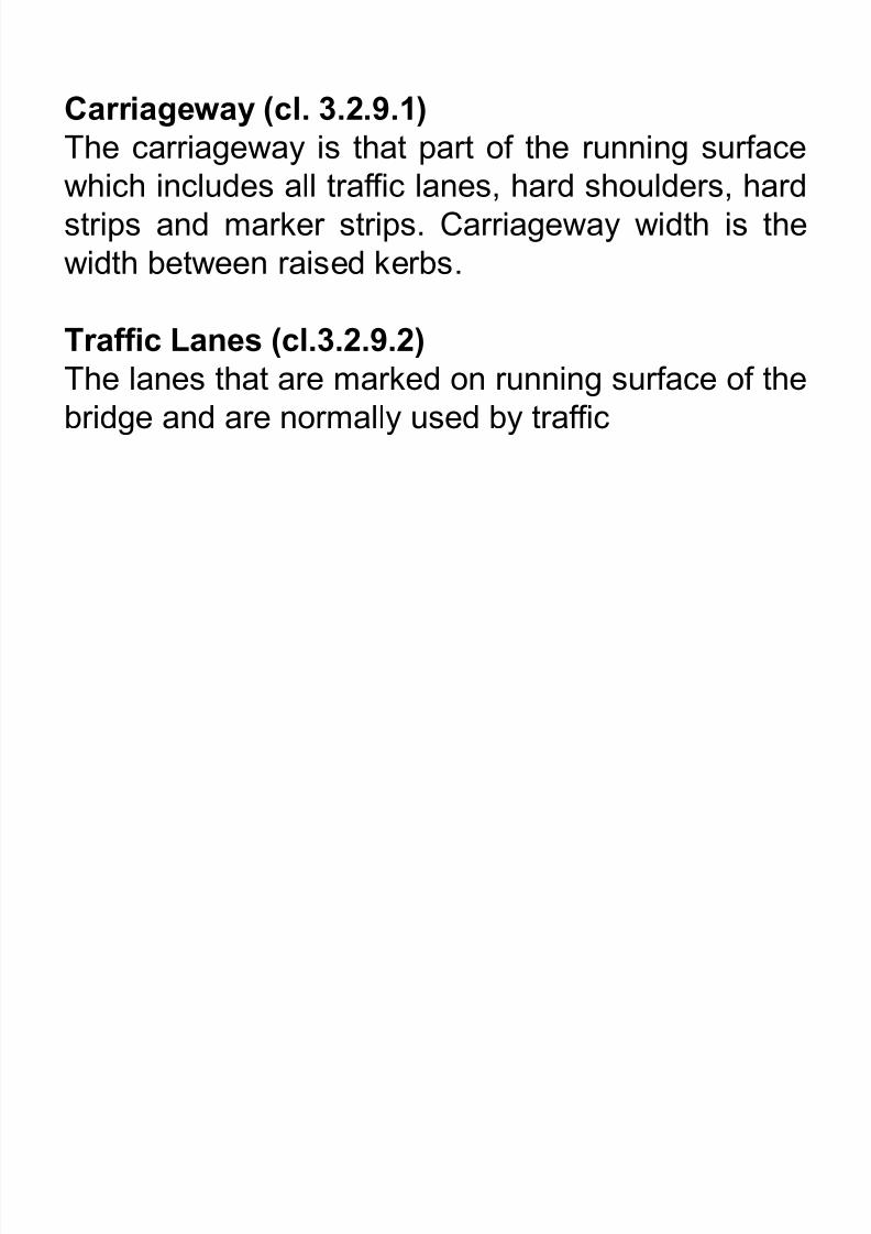
Carriageway (cl. 3.2.9.1)

The carriageway is that part of the running surfacewhich includes all traffic lanes, hard shoulders, hard

strips and marker strips. Carriageway width is the

width between raised kerbs.

Traffic Lanes (cl.3.2.9.2)

The lanes that are marked on running surface of the

bridge and are normally used by traffic



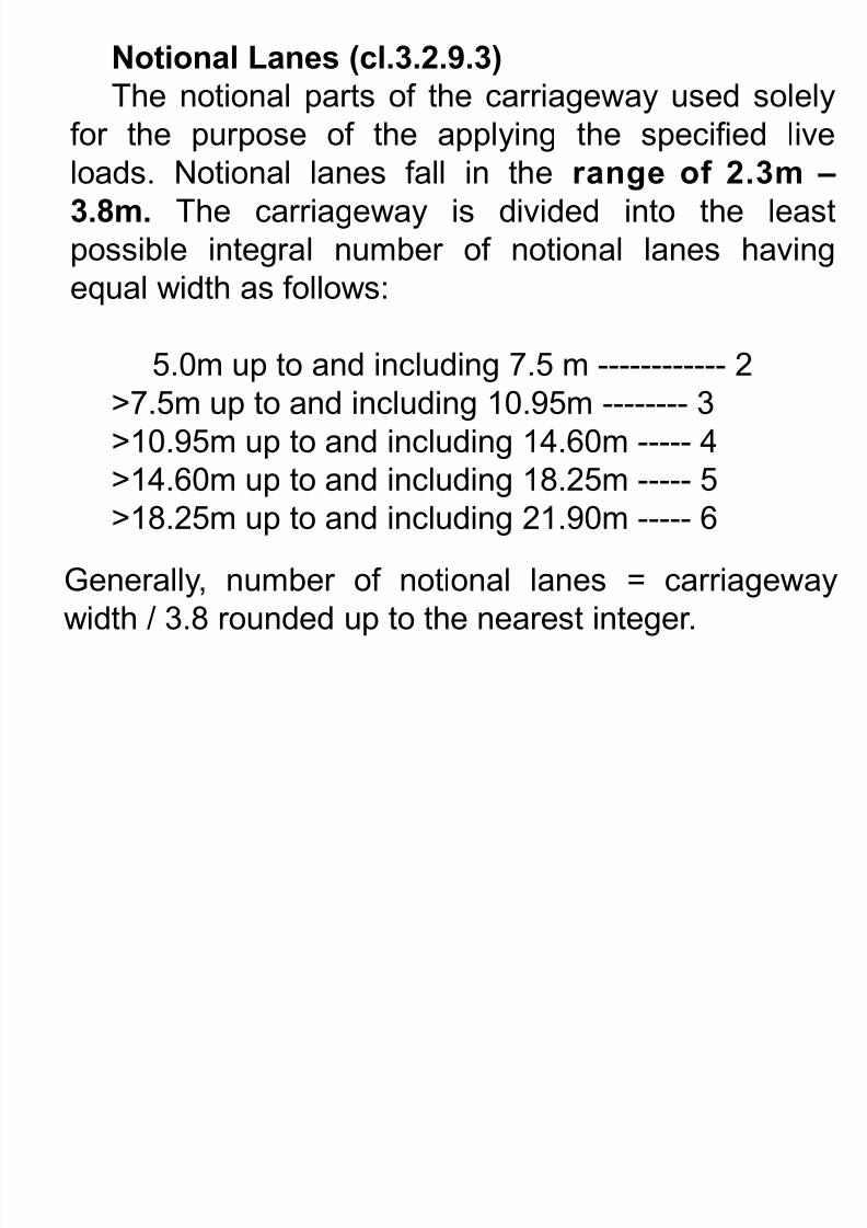
Notional Lanes (cl.3.2.9.3)

The notional parts of the carriageway used solely

for the purpose of the applying the specified live

loads. Notional lanes fall in the range of 2.3m ±

3.8m. The carriageway is divided into the least

possible integral number of notional lanes having

equal width as follows:

5.0m up to and including 7.5 m ------------ 2

>7.5m up to and including 10.95m -------- 3

>10.95m up to and including 14.60m ----- 4>14.60m up to and including 18.25m ----- 5

>18.25m up to and including 21.90m ----- 6

Generally, number of notional lanes = carriageway

width / 3.8 rounded up to the nearest integer.



2.3.1.8.1 HA Loading Alone

The full HA is applied to the first two notional lanes

(cl.6.4.1) in the appropriate parts of the influence

line for the element or member under consideration

and HA applied to all other lanes, except where

otherwise specified by the authority. HAK is applied

once in the loaded length.

is a factor which accounts for the attenuation of traffic loading in the transverse direction. Further

information is given in Table 14 of the Standard BD

37/88.



.3.1.8.2 HA and HB Combined (cl. 6.4.2)

Figure 13 of Standard BD 37/88 describes how to

combine HA and HB loading for global analysis



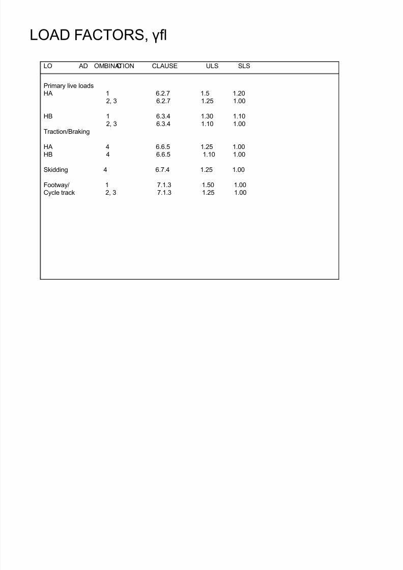
LO AD COMBINATION CLAUSE ULS SLS

Primary live loadsHA 1 6.2.7 1.5 1.20

2, 3 6.2.7 1.25 1.00

HB 1 6.3.4 1.30 1.102, 3 6.3.4 1.10 1.00

Traction/Braking

HA 4 6.6.5 1.25 1.00HB 4 6.6.5 1.10 1.00

Skidding 4 6.7.4 1.25 1.00

Footway/ 1 7.1.3 1.50 1.00Cycle track 2, 3 7.1.3 1.25 1.00

LO AD F ACTORS, fl



2.3.2 US Specification and Loading Systems

In the United States, highway loads are based on

the American Association of State Highway and

Transportation Officials (AASHTO) Standard

Specification for Highway Bridges 1996.

The specification stipulates two truck loading

systems and a tandem (a pair of axles) of the

military type, all of which must be consideredseparately with a constant lane load of 9.3kN/m,

which is irrespective of loaded length.



2.3.2.1 Truck Loading Systems

The truck loading is divided into classes: the Hloadings and the HS loading, both of which are

shown in Fig 3.1.1.

The H loadings represent an idealized standardtwo-axle truck; the HS loadings represent a two-

axle tractor and a single axle semi-trailer

combination with variable spacing between the two

rear axles (4.2m to 20m).



Each truck loading system consists of two vehicles:

the H system has the HL15-93 and the HL20-93

trucks, while the HS system has the HLS 15-93 andHLS 20-93 trucks.

The number following the standard truck

specification HL or HLS refers to the gross weightof the truck in tons, and the affix indicates the year

the loading was specified.

In the

Fig,

Wrepresents the total weight of the truckand load in ton for the HL trucks or the loaded

weight of the tractor in the HLS loading.

The tandem loading consist of a pair of axles which

are 1.2m apart, each weighing 110kN.



2.3.2.2 Selection of Loadings

The AASHTO specifications provide that bridges

supporting interstate highways shall be designedfor HLS 20- 93 loading or the tandem loading,

whichever produces the greatest stress.

For other highways that may carry heavy truck

traffic the minimum live load shall be HLS 15-93.



2.3.2.3 Application of Loadings

The lane together with standard truck or tandem

loading shall be assumed to occupy a width of

3.0m.

These loads shall be placed in 3.6m wide design

traffic lanes spaced across the entire bridge

roadway in numbers and positions required toproduce the maximum stress. Roadway widths

from 6m to 7.2m shall have two design lanes, each

equal to one half the roadway width.

Each loading shall be considered as a unit, and

fractional load-lane widths or fractional trucks shall

not be used.



Where maximum stresses are produced in anymember by loading any number of traffic lanes

simultaneously, the following multiple presence

factors are to be used to modify the live load

stresses according to the number of design trafficlanes:

Single lane 1.2

Two lanes 1.0Three lanes 0.85

Four lanes and above 0.65



The multiple presence factor takes account of the

improbable coincidence of the design truck being

present in all the lanes at the same time.

The minimum distance between the wheels of two

adjacent trucks is 1.2m.

The minimum distance from the centre of the wheel

to the face of parapet is 300mm.



2.3.2.4 Dynamic Effects

Dynamic effects due to irregularities in the road

surface and different suspension systems magnifythe static effects of the live loads.

This is taken care of by an impact factor called

dynamic load allowance (DLA) defined as

DLA=Ddyn / Dsta

Where, Dsta is the static deflection under live loads,

and Ddyn is the additional dynamic deflection under

live loads.



Dynamic live load effect = (static live load effect) x

(1+DLA). (1.33 typical for truck loading)

Values of DLA are given in the AASHTO

Specification for individual bridge components.



2.3.2.5 Longitudinal Loads

According to the specifications, the braking force

shall be taken as the greater of 25% of the axle

weight of the design truck or design tandem

OR

5% of the design truck plus lane load or 5% of the

design tandem plus lane load.

The braking force is placed in all design lanes,

which are considered to be loaded, with traffic

heading in the same direction.



The forces are assumed to act horizontally at aheight 1.8m above the roadway surface in either

longitudinal direction to cause the extreme force

effects.



2.3.2.6 Partial Load Factors

Design is carried out based on either permissiblestresses or limit state philosophy with partial safety

factors.

The following factors were obtained from workcarried out for the Federal Highway Administration

[1] based on AASHTO-LRFD (Load and Resistance

Factor Design) Specification.



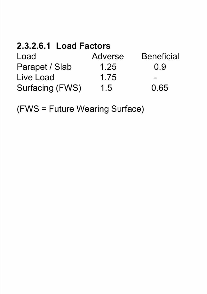
2.3.2.6.1 Load Factors

Load Adverse Beneficial

Parapet / Slab 1.25 0.9

Live Load 1.75 -Surfacing (FWS) 1.5 0.65

(FWS = Future Wearing Surface)



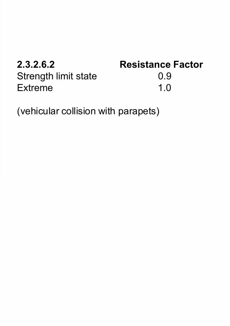
2.3.2.6.2 Resistance Factor

Strength limit state 0.9

Extreme 1.0

(vehicular collision with parapets)

Documents

Ivovi's Lecture 1