Jeffrey, M. R., & Glendinning, P. (2012). Grazing-sliding bifurcations,the border collision normal form, and the curse of dimensionality fornonsmooth bifurcation theory. Manuscript in preparation.

Early version, also known as pre-print

Link to publication record in Explore Bristol ResearchPDF-document

University of Bristol - Explore Bristol ResearchGeneral rights

This document is made available in accordance with publisher policies. Please cite only thepublished version using the reference above. Full terms of use are available:http://www.bristol.ac.uk/red/research-policy/pure/user-guides/ebr-terms/

Grazing-sliding bifurcations, the border collision normal form,

and the curse of dimensionality for nonsmooth bifurcation theory

Paul Glendinning∗

Centre for Interdisciplinary Computational and Dynamical

Analysis (CICADA) and School of Mathematics,

University of Manchester, Manchester, M13 9PL, U.K.

Mike R. Jeffrey†

Department of Mathematical Sciences, University of Bath, Claverton Down, Bath, BA2 7AY, U.K.

In this paper we show that the border collision normal form of continuous but non-

differentiable discrete time maps is affected by a curse of dimensionality: it is impossible

to reduce the study of the general case to low dimensions, since in every dimension the bifur-

cation produces fundamentally different attractors (contrary to the case of smooth systems).

In particular we show that the n-dimensional border collision normal form can have invariant

sets of dimension k for integer k from 0 to n. We also show that the border collision normal

form is related to grazing-sliding bifurcations of switching dynamical systems. This implies

that the dynamics of these two apparently distinct bifurcations (one for discrete time dy-

namics, the other for continuous time dynamics) are closely related and hence that a similar

curse of dimensionality holds for this bifurcation.

PACS numbers: 05.45.-a

Keywords: non-smooth bifurcation, attractor, grazing-sliding, border-collision, piecewise smooth

systems

I. INTRODUCTION

Despite their obvious lack of appeal analytically, piecewise-smooth differential equations have

found application in mechanics, biological modelling, computer science, control, and electrical

engineering. Under generic conditions, the bifurcations that such models can undergo, so-called

discontinuity induced bifurcations, are known to fit within a reasonably small number of normal

forms, prominent amongst which are the sliding bifurcations in non-differentiable flows [4], and the

border collisions in non-differentiable maps [2, 14]. Except in low dimensional cases there is still no

∗Electronic address: p.a.glendinning@manchester.ac.uk†Electronic address: mike.jeffrey@bristol.ac.uk

2

obvious classification of the dynamics near these bifurcations and there is a risk, in consequence,

that the literature becomes filled with ever more complicated examples.

In this paper we show that there is a link between two of these normal forms, in the sense

that one of them arises as an induced map in the analysis of the other. We hope that this is

the beginning of a more coherent description of the inter-relatedness of different models, and in

particular, that this will aid in the understanding of bifurcations in high dimensional nonsmooth

systems. We also discuss the possible attractors that can occur in these models. Our results suggest

that the bifurcation theory of piecewise-smooth systems suffers from the curse of dimensionality

[1], in that the description of a bifurcation on Rn depends crucially on n. This is in marked contrast

to the case of local bifurcation theory for smooth systems, where the centre manifold theorem (see

e.g. [10]) ensures that only the eigenvectors and eigenvalues, together with some genericity and

transversality conditions, determine any invariant sets that are created at the bifurcation.

The border collision normal form, derived by Nusse and Yorke [14] in two-dimensions, and by

di Bernardo [2, 5] in higher dimensions, describes bifurcations of fixed points in non-differentiable

maps. It arises when phase space is divided into two regions by a switching surface, and differ-

entiable discrete time dynamics is defined separately in each region, by maps that are continuous

across the switching surface but whose Jacobians may be discontinuous. If a fixed point in one

region varies with changing parameters so that it lies on the switching surface, then a border col-

lision is said to occur. The normal form is a piecewise linear map. This has been studied in its

own right before its appearance as a normal form in piecewise-smooth systems, see e.g. [13], and

its two dimensional normal form is

z′1

z′2

=

AL

z1

z2

+

ν

0

if z1 < 0

AR

z1

z2

+

ν

0

if z1 > 0

(1)

where

AL =

TL 1

−DL 0

, AR =

TR 1

−DR 0

. (2)

In higher dimensions (Rn) the map remains affine and both AL and AR can be put into observer

3

canonical form [2]

Aj =

ωj1 1 0 . . . 0 0

ωj2 0 1 . . . 0 0

ωj3 0 0 . . . 0 0...

....... . .

......

ωj(n−1) 0 0 . . . 0 1

ωjn 0 0 . . . 0 0

, (3)

with j taking the two labels L and R (so wj1 = Tj and wj2 = −Dj in two dimensions), while the

obvious additive constant becomes the column vector with components

(ν, 0, 0, . . . , 0, 0).

Note that only the sign of ν can influence the dynamic behaviour of the model: by a linearly

rescaling of the variables zj the parameter ν may be chosen without loss of generality to be either

−1, 0, or 1.

The grazing-sliding normal form describes a bifurcation of piecewise-smooth flows (Filippov

systems). As in the border collision normal form, phase space is divided into two regions by a

switching surface, and in this case, differentiable continuous time dynamics is defined separately

in each region by ordinary differential equations. If a periodic orbit in one region becomes tangent

to the switching surface at an isolated point and some critical value of a parameter, and the vector

field defining the dynamics in the other region points towards the switching surface at this point, a

grazing-sliding bifurcation is said to occur. The term sliding refers to nearby solutions that typically

include segments of sliding along the switching surface. In two dimensions these bifurcations can

be described relatively easily [4, 12], but in three dimensions the situation is already considerably

more complicated [7, 8]. Here we consider the case of grazing-sliding bifurcations in Rn, n ≥ 4.

In the next section we describe the conditions for a grazing-sliding bifurcation to occur in

piecewise-smooth systems in Rn (see e.g. [4]), and show how to reduce this to an (n−2)-dimensional

return mapping, following the procedure adopted in [7] for n = 3. In section III we treat the four

dimensional case, showing the formal reduction to the border collision normal form (1), under cer-

tain conditions. In section IV we give specific examples that show these conditions can be satisfied.

Sections IV and V generalize the previous two sections to higher dimensions. In section VII we

describe how the n-dimensional border collision normal form of di Bernardo [2] can have invariant

sets of any given non-negative integer dimension less than or equal to n.

4

II. GRAZING-SLIDING IN Rn

The piecewise-smooth systems we consider are defined by two sets of smooth differential equa-

tions whose regions of definition are separated by a smooth manifold Σ, the switching surface. We

write these as

(x, y, z) =

f+(x, y, z;µ) if h(x, y, z;µ) > 0,

f−(x, y, z;µ) if h(x, y, z;µ) < 0,(4)

where f± are smooth functions of the variables (x, y, z) and a parameter µ. It is useful to think

of f+ and f− each being defined on the whole of Rn. We have separated out x, y ∈ R, and

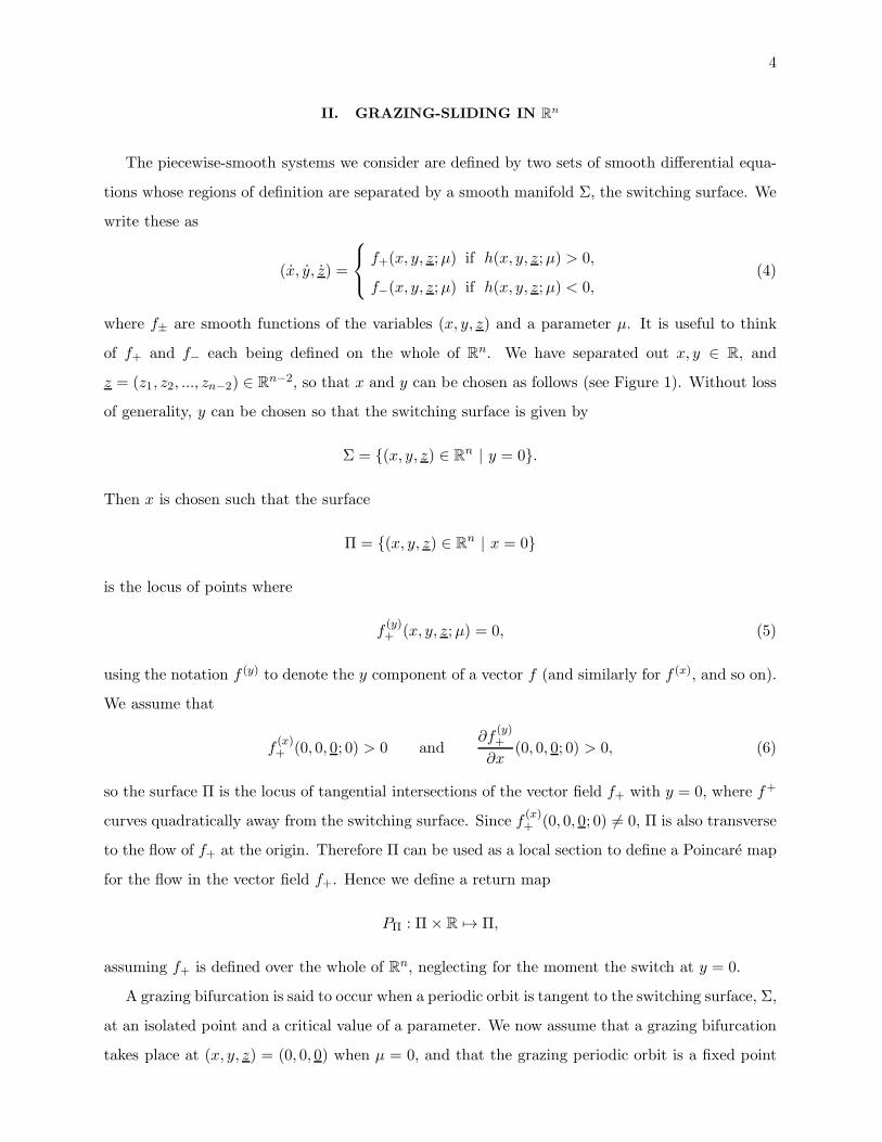
z = (z1, z2, ..., zn−2) ∈ Rn−2, so that x and y can be chosen as follows (see Figure 1). Without loss

of generality, y can be chosen so that the switching surface is given by

Σ = {(x, y, z) ∈ Rn | y = 0}.

Then x is chosen such that the surface

Π = {(x, y, z) ∈ Rn | x = 0}

is the locus of points where

f(y)+ (x, y, z;µ) = 0, (5)

using the notation f (y) to denote the y component of a vector f (and similarly for f (x), and so on).

We assume that

f(x)+ (0, 0, 0; 0) > 0 and

∂f(y)+

∂x(0, 0, 0; 0) > 0, (6)

so the surface Π is the locus of tangential intersections of the vector field f+ with y = 0, where f+

curves quadratically away from the switching surface. Since f(x)+ (0, 0, 0; 0) 6= 0, Π is also transverse

to the flow of f+ at the origin. Therefore Π can be used as a local section to define a Poincare map

for the flow in the vector field f+. Hence we define a return map

PΠ : Π× R 7→ Π,

assuming f+ is defined over the whole of Rn, neglecting for the moment the switch at y = 0.

A grazing bifurcation is said to occur when a periodic orbit is tangent to the switching surface, Σ,

at an isolated point and a critical value of a parameter. We now assume that a grazing bifurcation

takes place at (x, y, z) = (0, 0, 0) when µ = 0, and that the grazing periodic orbit is a fixed point

5

of the map PΠ. We also assume a parametric transversality condition, namely that the fixed point

of PΠ moves through y = 0 with non-zero velocity as µ passes through zero; more detail is given

the Appendix (see also [3, 4]).

Π

Σ

x

sliding

(i) (ii)y

zi

x

y

zi

f+

f−

P∏P

∏

P∏

PDM

Π

Σ

P∏

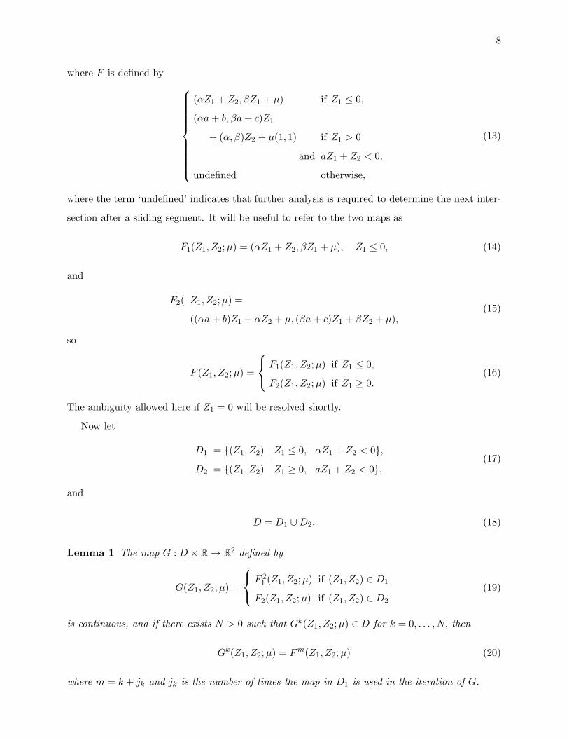
FIG. 1: (i) The grazing periodic orbit, in coordinates (x, y, z) = (x, y, (z1, z2, ...)), with vector fields f+ and

f−

either side of the switching surface Σ. (ii) The return map PΠ on Π is valid for y > 0, and in y < 0 a

correction PDM accounts for the occurence of sliding.

Whilst the flow in y > 0 defines the grazing part of a grazing-sliding bifurcation, the sliding

part is furnished by also considering the properties of f−. We assume f(y)− (0, 0, 0; 0) > 0, so that

f− points locally towards Σ. Considering also the sign of f(y)+ , by (5) we have f

(y)+ (x, 0, z;µ) < 0 in

x < 0, so that there is a region of values of x on Σ on which both vector fields f± point towards Σ.

This confines the flow of (4) to a sliding component on Σ, which is generally modelled by taking

the linear combination of f+ and f− that lies tangent to Σ. This sliding motion terminates on the

surface x = 0 (in y = 0) where f(y)+ changes sign, so that when it reaches Π the flow lifts off from

Σ back into y > 0.

Details of how to define sliding solutions are given in any standard text (e.g. [5, 6], see also

Appendix A). The important point now is that, when sliding is taken into account, we can reduce

the model of the dynamics near the grazing orbit to an (n − 2)-dimensional return map on the

surface Π∩Σ (x = y = 0). The return map PΠ : Π 7→ Π neglects the switch at y = 0, in particular

the sliding motion that brings the flow to x = 0. This is easily corrected by composing PΠ with a

local reset

PDM : Π× R → Π ∩ Σ,

called a Poincare Discontinuity Map [4]. The parameter dependence of PDM lies in the nonlinear

terms, so the linearization of the PDM used below is independent of the parameter. The composition

PDM ◦P kΠ, for appropriate k (where the y-component of P k

Π lies in y < 0), gives a µ-parameterized

return map on the set Π∩Σ, which is the intersection of the return plane Π with the sliding surface

6

on Σ, and also the locus of solutions that lift off into y > 0 from the sliding surface. This map is

piecewise continuous (discontinuities corresponding to orbits undergoing grazing). Essentially PΠ

is applied to a point (0, 0, z) ∈ Π∩Σ, and iterated until the y-component of P kΠ(0, 0, z;µ) becomes

negative for the first time. Then PDM is applied to bring the solution back to where it would have

intersected Π ∩ Σ had the sliding component been taken into account.

This informal account is enough to make the following sections comprehensible if the reader is

prepared to take the stated linearizations of PΠ and PDM on trust. The omitted details are given in

the Appendix, together with a discussion about the choice of coordinates. In particular, regarding

the Poincare map PΠ, we are implicitly assuming here that, except for the point (x, y, z) = (0, 0, 0),

the grazing periodic orbit lies only in y > 0. This can be relaxed to allow entry to y ≤ 0 far away

from (x, y, z) = (0, 0, 0), provided certain transversality conditions, and we remark on this in Section

VIII. Regarding the discontinuity map PDM , a peculiarity of grazing-sliding is that the derivative

of PDM is nonzero at y = 0, in contrast to the maps associated with other codimension one sliding

bifurcations [4, 5], implying that they are not affected by much of the interesting behaviour that

we find here for grazing-sliding. In the next section we give explicit forms for PΠ and PDM in four

dimensions, followed by examples, before giving general n-dimensional forms in Section V.

III. GRAZING-SLIDING BIFURCATIONS IN FOUR DIMENSIONS

Consider a system of four variables (x, y, z1, z2) ∈ R4 as described in the previous section, so that

they vary in time forming a periodic orbit that grazes from y > 0 when µ = 0. The linearization

of the return map PΠ close to the periodic orbit can be described in observer canonical form (see

Appendix A) as

y′

z′1

z′2

=

a 1 0

b 0 1

c 0 0

y

z1

z2

+ µ

1

0

0

. (7)

After each iteration, if y′ > 0 then the flow misses the switching surface and the map is iterated

again. If y′ < 0 then PΠ neglects the fact that the flow has reached the switching surface a little

before the intersection with x = 0. To correct this, the value of y′ needs to be adjusted using

the Poincare Discontinuity Map to take the solution back to the sliding surface y = 0, and then

evolve it along the switching surface to the next point at which the solution can leave the sliding

surface, viz. x = y = 0. Expanding solutions as power series in the (small) time taken to make

7

this adjustment leads to the general form for the linearization of PDM

y′′

z′′1

z′′2

=

0 0 0

α 1 0

β 0 1

y′

z′1

z′2

. (8)

If a solution starts on the surface Π with y = 0 (the ‘lift-off’ surface Π∩Σ), the return map (7)

brings the trajectory from (0, z1, z2) back to Π at

(z1 + µ, z2, 0).

If z1 + µ < 0, the linearized Poincare discontinuity mapping (8) brings the solution back to x = 0

with

(z′′1 , z′′2 ) = (α(z1 + µ) + z2, β(z1 + µ)). (9)

If z1 + µ > 0 then the modelled trajectory lies entirely in y > 0 during this part of its motion and

the return map (7) is applied again, giving

(a(z1 + µ) + z2 + µ, b(z1 + µ) + z2, c(z1 + µ)).

Now, if a(z1+µ)+z2+µ > 0 the solution goes round in y > 0 again, whilst if a(z1+µ)+z2+µ < 0

(8) is applied to find the next intersection with y = 0 (i.e. Σ) on the surface x = 0 (i.e. Π), which

is

(z′′1 , z′′2 ) = (αa+ b, βa+ c)(z1 + µ)

+(α, β)(z2 + µ) + (z2, 0).(10)

Thus, writing Z1 = z1 + µ and Z2 = z2 + µ, the dynamics of solutions that go once or twice round

the cycle in y > 0 before having a sliding segment can be described by the maps

(z′′1 , z′′2 ) =

(α, β)Z1 + (Z2 − µ, 0) if Z1 < 0,

(α, β)(aZ1 + Z2) + (b, c)Z1 if Z1 > 0

and aZ1 + Z2 < 0,

undefined otherwise.

(11)

Writing these evolution equations using coordinates Z1 and Z2 throughout and replacing the iter-

ation double primes with single primes, we obtain

(Z ′1, Z

′2) = F (Z1, Z2;µ) (12)

8

where F is defined by

(αZ1 + Z2, βZ1 + µ) if Z1 ≤ 0,

(αa+ b, βa+ c)Z1

+ (α, β)Z2 + µ(1, 1) if Z1 > 0

and aZ1 + Z2 < 0,

undefined otherwise,

(13)

where the term ‘undefined’ indicates that further analysis is required to determine the next inter-

section after a sliding segment. It will be useful to refer to the two maps as

F1(Z1, Z2;µ) = (αZ1 + Z2, βZ1 + µ), Z1 ≤ 0, (14)

and

F2( Z1, Z2;µ) =

((αa + b)Z1 + αZ2 + µ, (βa+ c)Z1 + βZ2 + µ),(15)

so

F (Z1, Z2;µ) =

F1(Z1, Z2;µ) if Z1 ≤ 0,

F2(Z1, Z2;µ) if Z1 ≥ 0.(16)

The ambiguity allowed here if Z1 = 0 will be resolved shortly.

Now let

D1 = {(Z1, Z2) | Z1 ≤ 0, αZ1 + Z2 < 0},

D2 = {(Z1, Z2) | Z1 ≥ 0, aZ1 + Z2 < 0},(17)

and

D = D1 ∪D2. (18)

Lemma 1 The map G : D × R → R2 defined by

G(Z1, Z2;µ) =

F 21 (Z1, Z2;µ) if (Z1, Z2) ∈ D1

F2(Z1, Z2;µ) if (Z1, Z2) ∈ D2

(19)

is continuous, and if there exists N > 0 such that Gk(Z1, Z2;µ) ∈ D for k = 0, . . . , N, then

Gk(Z1, Z2;µ) = Fm(Z1, Z2;µ) (20)

where m = k + jk and jk is the number of times the map in D1 is used in the iteration of G.

9

Note that if Gk(Z1, Z2;µ) = (0, ζ) for some ζ then there is a choice about whether to apply the

map defined in D1 or the map in D2. We assume in the statement of the lemma that the same

choice is made in the evaluation of both G and F . The continuity of G implies that this makes no

difference to the eventual orbit (this is the inevitable ambiguity of a grazing solution).

The importance of this lemma is that it implies that if G has an attractor in D then there is a

corresponding attractor of F in {Z1 ≤ 0}∪D2, and the action of G restricted to this set is linearly

conjugate to the attractor of a border collision normal form with appropriately chosen parameters.

These results are formalized in Corollaries 2 and 3 below.

Proof of Lemma 1: If (Z1, Z2) ∈ D1 then F (Z1, Z2;µ) = F1(Z1, Z2;µ) = (αZ1 + Z2, βZ1 + µ)

and so F1(Z1, Z2;µ) ∈ {Z1 ≤ 0} by the definition of D1 and F 2(Z1, Z2;µ) = F (F1(Z1, Z2;µ);µ) =

F 21 (Z1, Z2;µ) and by direct calculation this is

((α2 + β)Z1 + αZ2 + µ, αβY + βZ2 + µ), (Z1, Z2) ∈ D1. (21)

In particular, F 21 is well defined for (Z1, Z2) ∈ D1. Since F1 and F2 are continuous, G is continuous

provided it is continuous on Z1 = 0, and by (21)

F 21 (0, Z1;µ) = (αZ2 + µ, βZ2 + µ) = F2(0, Z2;µ)

where the second equality follows from (15). Hence G is continuous and the equality (20) follows

as G = F 2 on D1 and G = F on D2.

�

Corollary 2 If G|D has an attracting set then F has an attracting set in {Z1 ≤ 0} ∪D2.

This is obvious from Lemma 1.

Corollary 3 If G|D has an attracting set then G|D is linearly conjugate to the border collision

normal form restricted to some appropriate domain E ⊆ R2 containing at least one attractor. The

parameters of the border collision normal form can be chosen so that

AL =

α2 + 2β 1

−β2 0

AR =

αa+ b+ β 1

−(βb− αc) 0

(22)

with sign(ν) = sign(µ), where ν corresponds to the parameter of the border collision normal form

as in (1).

10

1

0

-1

0.50-0.5

)0

1

2

3

-1 0 1 2 3 4

(ii)

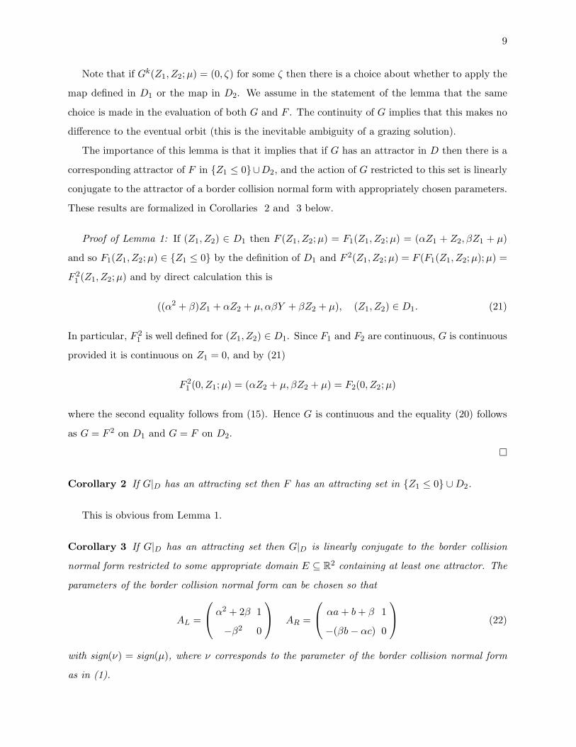
FIG. 2: The thin attractor. (i) The attractor of grazing sliding map with parameters (23) also showing the

boundary of D. (ii) The attractor of the border collision normal form with parameters (24)

.

Proof: The determinant and trace of the two linear maps (15) and (21) are easy to calculate and

the coordinate changes are essentially those used by Nusse and Yorke to obtain the normal form

[14]. (The first column of the border collision normal form is the trace and minus the determinant

of the map.) The only complication is the sign of µ (by a linear rescaling it is only the sign of µ

that determines the dynamics), and this follows from the observation that G(0, 0;µ) = (µ, µ) which

is in D2 if µ > 0 and Z1 ≤ 0 if µ < 0. The corresponding point for the border collision normal

form is also (0, 0), hence the result.

�

IV. TWO EXAMPLES

The results of the previous section establish a formal connection between the attractors of the

linearized grazing-sliding normal form F , an induced map G and the border collision normal form.

However, the attractor of Gmust lie in the region D of equation (18) for the results to be applicable,

and we have not established conditions for this to be the case. In particular it might never be the

case!

In this section we show numerically that there are attractors with the desired properties, and

hence that the there is content in the results described above. The two examples are chosen to

illustrate different geometries of the attractor – in the first the attractor is nearly a union of curves

(though it actually appears to have a fractal structure) and in the second the attractor occupies a

much larger region of phase space.

11

0

1

-1

-2 -1 0 1

) (ii)

0

2

4

420-2

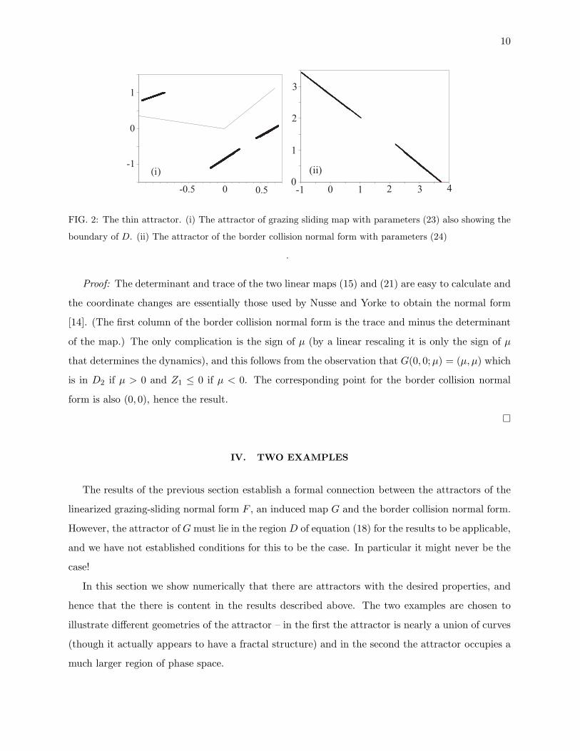
FIG. 3: The thick attractor, as Figure 2 but using parameters (25) and (26).

The first example is illustrated in Figure 2. This has parameters

a = −1.6, b = −1.15, c = −1.15,

α = 0.3, β = 1.1, µ = 1;(23)

for F , which translate to

TL = 2.29, DL = 1.21, TR = −0.53,

DR = −0.92, ν = 1;(24)

for the border collision normal form, with TL the trace of AL, DL the determinant of AL and

similarly for AR. The attractor of F is shown in Figure 2(i) (and the attractor for G is the part

shown in the region D), whilst the attractor of the corresponding border collision normal form is

shown in Figure 2(ii).

The second example is illustrated in Figure 3 with the same layout and

a = −1.8, b = −1.4, c = −1.4,

α = 0.4, β = 1.2, µ = 1;(25)

for F , which translate to

TL = 2.56, DL = 1.44, TR = −0.92,

DR = −1.12, ν = 1;(26)

V. THE GENERAL CASE

The results of section III used a special choice for the return map of the grazing orbit and

restricted to only four dimensions, leading to a two-dimensional model. This was done so that the

geometry could be easily appreciated and examples found. In this section we consider the general

12

case, both in terms of the return map and the dimension, and show that results analogous to those

of section III hold again, with the border collision normal form of Nusse and Yorke replaced by the

(n− 2)−dimensional generalization of di Bernardo [2, 5].

The following two Lemmas express these in a convenient form, without loss of generality.

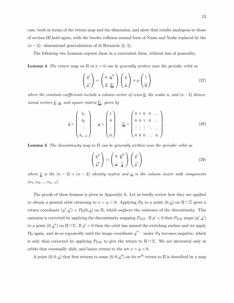
Lemma 4 The return map on Π in x > 0 can be generally written near the periodic orbit as

y′

z′

=

a uT

b U

y

z

+ µ

1

0

(27)

where the constant coefficients include a column vector of zeros 0, the scalar a, and (n− 2) dimen-

sional vectors b, u, and square matrix U , given by

b =

b1

b2...

bn−2

, u =

1

0...

0

, U =

0 1 0 0 . . .

0 0 1 0 . . .

......

.... . . . . .

0 0 0 . . . 0

. (28)

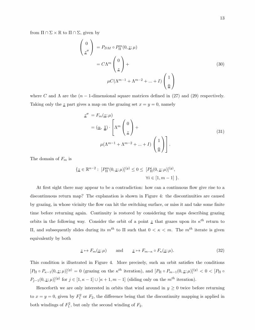
Lemma 5 The discontinuity map to Π can be generally written near the periodic orbit as

y′′

z′′

=

0 0T

α 1

y′

z′

(29)

where 1 is the (n − 2) × (n − 2) identity matrix and α is the column vector with components

(α1, α2, ..., αn−1).

The proofs of these lemmas is given in Appendix A. Let us briefly review how they are applied

to obtain a general orbit returning to x = y = 0. Applying PΠ to a point (0, z) on Π ∩ Σ gives a

return coordinate (y′, z′) = PΠ(0, z) on Π, which neglects the existence of the discontinuity. This

omission is corrected by applying the discontinuity mapping PDM . If y′ < 0 then PDM maps (y′, z′)

to a point (0, z′′) on Π∩Σ. If y′ > 0 then the orbit has missed the switching surface and we apply

PΠ again, and do so repeatedly until the image coordinate y′′′··· under PΠ becomes negative, which

is only then corrected by applying PDM to give the return to Π ∩ Σ. We are interested only in

orbits that eventually slide, and hence return to the set x = y = 0.

A point (0, 0, z) that first returns to some (0, 0, z′′) on its mth return to Π is described by a map

13

from Π ∩ Σ× R to Π ∩ Σ, given by

0

z′′

= PDM ◦ PmΠ (0, z;µ)

= CΛm

0

z

+

µC(Λm−1 + Λm−2 + ...+ I)

1

0

(30)

where C and Λ are the (n − 1-dimensional square matrices defined in (27) and (29) respectively.

Taking only the z part gives a map on the grazing set x = y = 0, namely

z′′ = Fm(z;µ)

= (α, 1) ·

Λm

0

z

+

µ(Λm−1 + Λm−2 + ...+ I)

1

0

.

(31)

The domain of Fm is

{z ∈ Rn−2 : [Pm

Π (0, z;µ)](y) ≤ 0 ≤ [P iΠ(0, z;µ)]

(y),

∀i ∈ [1,m− 1] }.

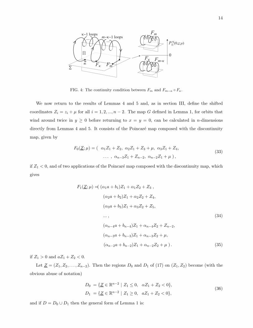
At first sight there may appear to be a contradiction: how can a continuous flow give rise to a

discontinuous return map? The explanation is shown in Figure 4: the discontinuities are caused

by grazing, in whose vicinity the flow can hit the switching surface, or miss it and take some finite

time before returning again. Continuity is restored by considering the maps describing grazing

orbits in the following way. Consider the orbit of a point z that grazes upon its κth return to

Π, and subsequently slides during its mth to Π such that 0 < κ < m. The mth iterate is given

equivalently by both

z 7→ Fm(z;µ) and z 7→ Fm−κ ◦ Fκ(z;µ). (32)

This condition is illustrated in Figure 4. More precisely, such an orbit satisfies the conditions

[PΠ ◦ Pκ−1(0, z;µ)](y) = 0 (grazing on the κth iteration), and [PΠ ◦ Pm−1(0, z;µ)]

(y) < 0 < [PΠ ◦

Pj−1(0, z;µ)](y) for j ∈ [1, κ − 1] ∪ [κ+ 1,m− 1] (sliding only on the mth iteration).

Henceforth we are only interested in orbits that wind around in y ≥ 0 twice before returning

to x = y = 0, given by F 21 or F2, the difference being that the discontinuity mapping is applied in

both windings of F 21 , but only the second winding of F2.

14

�

∏

Fm

Fm

FκFm−κFκ

z

κ−1 loopsm−κ−1 loops

0

P∏

κ(0,z;µ)

FIG. 4: The continuity condition between Fm and Fm−κ ◦ Fκ.

We now return to the results of Lemmas 4 and 5 and, as in section III, define the shifted

coordinates Zi = zi + µ for all i = 1, 2, ..., n − 2. The map G defined in Lemma 1, for orbits that

wind around twice in y ≥ 0 before returning to x = y = 0, can be calculated in n-dimensions

directly from Lemmas 4 and 5. It consists of the Poincare map composed with the discontinuity

map, given by

F0(Z;µ) = ( α1Z1 + Z2, α2Z1 + Z3 + µ, α3Z1 + Z4,

. . . , αn−3Z1 + Zn−2, αn−2Z1 + µ ) ,(33)

if Z1 < 0, and of two applications of the Poincare map composed with the discontinuity map, which

gives

F1(Z;µ) =( (α1a+ b1)Z1 + α1Z2 + Z3 ,

(α2a+ b2)Z1 + α2Z2 + Z4,

(α3a+ b3)Z1 + α3Z2 + Z5,

... , (34)

(αn−4a+ bn−4)Z1 + αn−4Z2 + Zn−2,

(αn−3a+ bn−3)Z1 + αn−3Z2 + µ,

(αn−2a+ bn−2)Z1 + αn−2Z2 + µ ) . (35)

if Z1 > 0 and aZ1 + Z2 < 0.

Let Z = (Z1, Z2, . . . , Zn−2). Then the regions D0 and D1 of (17) on (Z1, Z2) become (with the

obvious abuse of notation)

D0 = {Z ∈ Rn−2 | Z1 ≤ 0, αZ1 + Z2 < 0},

D1 = {Z ∈ Rn−2 | Z1 ≥ 0, aZ1 + Z2 < 0},

(36)

and if D = D0 ∪D1 then the general form of Lemma 1 is:

15

Lemma 6 The map G : D × R → Rn−2 defined by

G(Z;µ) =

F 20 (Z;µ) if Z ∈ D0

F1(Z;µ) if Z ∈ D1

(37)

is continuous and if there exists N > 0 such that Gk(Z;µ) ∈ D for k = 0, . . . , N, then

Gk(Z;µ) = Fm(Z;µ) (38)

where m = k + jk and jk is the number of times the map in D0 is used in the iteration of G up to

the kth iterate.

Corollary 7 If G|D has an attracting set then G|D is linearly conjugate to the border collision

normal form restricted to some appropriate domain E ⊆ R2 containing at least one attractor.

VI. HIGH DIMENSIONAL EXAMPLES

As in the four dimensional case, the analysis of the previous section shows a correspondence

between solutions of the grazing-sliding normal form and the border collision normal form provided

that some conditions hold; in particular the attractor of the appropriate iterates of the grazing-

sliding normal form must lie in the region D1∪D2. As before, analytical conditions for the existence

of such an attractor have not been established. The aim of this section is to provide two examples,

one in 20 dimensions and one in 100 dimensions, to show that there are parameters at which these

conditions are satisfied. Both examples are extensions of the second example of section IV.

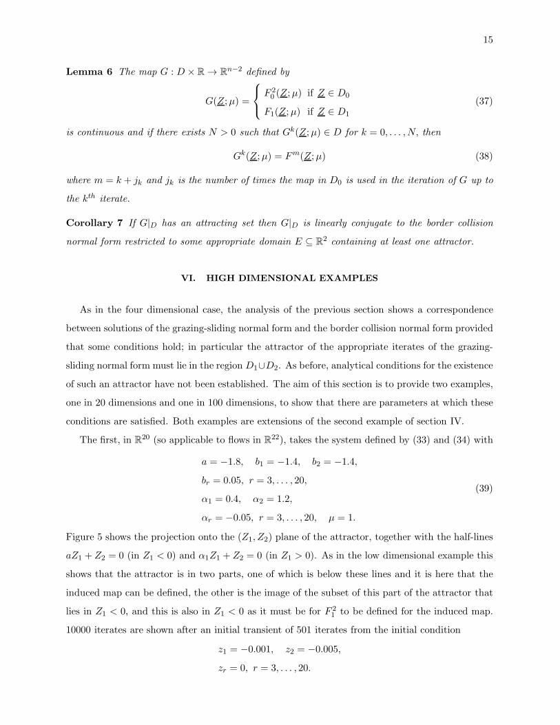
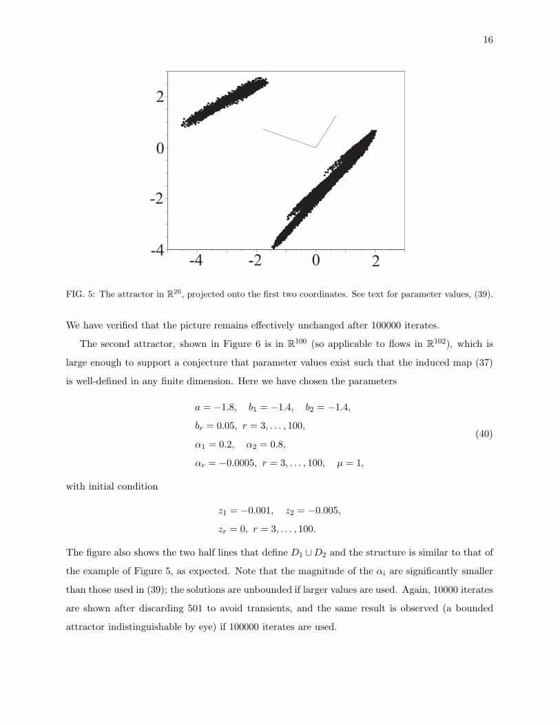
The first, in R20 (so applicable to flows in R

22), takes the system defined by (33) and (34) with

a = −1.8, b1 = −1.4, b2 = −1.4,

br = 0.05, r = 3, . . . , 20,

α1 = 0.4, α2 = 1.2,

αr = −0.05, r = 3, . . . , 20, µ = 1.

(39)

Figure 5 shows the projection onto the (Z1, Z2) plane of the attractor, together with the half-lines

aZ1 + Z2 = 0 (in Z1 < 0) and α1Z1 + Z2 = 0 (in Z1 > 0). As in the low dimensional example this

shows that the attractor is in two parts, one of which is below these lines and it is here that the

induced map can be defined, the other is the image of the subset of this part of the attractor that

lies in Z1 < 0, and this is also in Z1 < 0 as it must be for F 21 to be defined for the induced map.

10000 iterates are shown after an initial transient of 501 iterates from the initial condition

z1 = −0.001, z2 = −0.005,

zr = 0, r = 3, . . . , 20.

16

20-2-4-4

-2

0

2

FIG. 5: The attractor in R20, projected onto the first two coordinates. See text for parameter values, (39).

We have verified that the picture remains effectively unchanged after 100000 iterates.

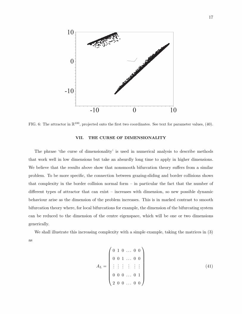
The second attractor, shown in Figure 6 is in R100 (so applicable to flows in R

102), which is

large enough to support a conjecture that parameter values exist such that the induced map (37)

is well-defined in any finite dimension. Here we have chosen the parameters

a = −1.8, b1 = −1.4, b2 = −1.4,

br = 0.05, r = 3, . . . , 100,

α1 = 0.2, α2 = 0.8,

αr = −0.0005, r = 3, . . . , 100, µ = 1,

(40)

with initial condition

z1 = −0.001, z2 = −0.005,

zr = 0, r = 3, . . . , 100.

The figure also shows the two half lines that define D1 ∪D2 and the structure is similar to that of

the example of Figure 5, as expected. Note that the magnitude of the αi are significantly smaller

than those used in (39); the solutions are unbounded if larger values are used. Again, 10000 iterates

are shown after discarding 501 to avoid transients, and the same result is observed (a bounded

attractor indistinguishable by eye) if 100000 iterates are used.

17

100-10

10

0

-10

FIG. 6: The attractor in R100, projected onto the first two coordinates. See text for parameter values, (40).

VII. THE CURSE OF DIMENSIONALITY

The phrase ‘the curse of dimensionality’ is used in numerical analysis to describe methods

that work well in low dimensions but take an absurdly long time to apply in higher dimensions.

We believe that the results above show that nonsmooth bifurcation theory suffers from a similar

problem. To be more specific, the connection between grazing-sliding and border collisions shows

that complexity in the border collision normal form – in particular the fact that the number of

different types of attractor that can exist – increases with dimension, so new possible dynamic

behaviour arise as the dimension of the problem increases. This is in marked contrast to smooth

bifurcation theory where, for local bifurcations for example, the dimension of the bifurcating system

can be reduced to the dimension of the centre eigenspace, which will be one or two dimensions

generically.

We shall illustrate this increasing complexity with a simple example, taking the matrices in (3)

as

AL =

0 1 0 . . . 0 0

0 0 1 . . . 0 0...

......

......

...

0 0 0 . . . 0 1

2 0 0 . . . 0 0

(41)

18

and

AR =

0 1 0 . . . 0 0

0 0 1 . . . 0 0...

......

......

...

0 0 0 . . . 0 1

−2 0 0 . . . 0 0

(42)

and letting ν = 1, so the constant term in the border collision normal form is

(1, 0, 0, . . . , 0, 0)T. (43)

Theorem 8 Consider the m-dimensional border collision normal form with AL and AR given by

(41), (42) and ν = 1. Then there is an invariant m-dimensional hypercube C such that: (a) the

Lebesgue measure is an invariant measure on C; (b) the Lyapunov exponent of almost all points is

positive on C; (c) periodic orbits are dense in C; (d) there is topological transitivity on C; and (e)

the map has sensitive dependence on initial conditions on C.

Proof: Let C be the hypercube with 2m vertices (u, v2, . . . , vm) with u ∈ {−1,+1} and vk ∈

{−2, 0}, k = 2, . . . ,m. The discontinuity surface z = 0 divides C into two cubes, C0 in z ≤ 0 and C1

in z ≥ 0, so C0 has vertices (u0, v2, . . . , vm) with u0 ∈ {−1, 0} and vk as before, and C1 has vertices

(u1, v2, . . . , vm) with u1 ∈ {0,+1}.

We will show that F (Cr) = C for r = 0, 1, (we omit the parameter from F since we have set

ν = 1), by looking at the action of the map on the vertices (since the map is affine, if the vertices

of Cr are mapped to those of C, then the whole of Cr maps to C).

Consider C0. The image of (u0, v2, . . . , vm) is

(v2 + 1, v3, . . . , vm, 2u0) (44)

and since v2 ∈ {−2, 0}, v2 + 1 ∈ {−1, 1}, and v3 to vm are each in {−2, 0}. Finally, 2u0 ∈ {−2, 0}

as u0 ∈ {−1, 0} and this shows that vertices of C0 map to vertices of C, clearly on a one-to-one

basis, and hence F (C0) = C. The argument for C1 is similar.

This establishes that C = C0 ∪ C1 is invariant and F (Cr) = C, r = 0, 1.

(a) Invariance of Lebesgue measure

First note that the modulus of the determinant of the linear part of the map describes how

volumes (Lebesgue measure, ℓ) is changed, so if B is a measurable set in x > 0 or in x < 0 then

ℓ(F (B)) = 2ℓ(B).

19

Since F (Cr) = C, r = 0, 1, for any measurable B ⊂ C there exist Pi ∈ Ci, i = 0, 1 such that

F (Pi) = B and ℓ(B) = 2ℓ(Pi). In other words

ℓ(B) = ℓ(P0) + ℓ(P1) = F−1(B)

which is the condition for a measure to be invariant under F .

(b) Positive Lyapunov exponents

This is a simple calculation. Iterating the relation (44) n times (bearing in mind that the

coefficient 2 could be either plus or minus two in the general case) shows that for a general point

x = (x1, x2, . . . , xn)

Fm(x) =

1 + σ12x1

σ22(1 + x2)...

σm2(1 + xm)

where σk ∈ {−1,+1}. Hence the linear part (the Jacobian) of the mth iterate of the map is

2diag(σ1, σ2, . . . , σm)

and hence every point in C has m Lyapunov exponents equal to 1mlog 2. (Note that this could be

deduced using the Cayley-Hamilton Theorem and the fact that the characteristic equation of the

linear parts of the map are λm ± 2 = 0.)

(c-e) Locally eventually onto (LEO)

We shall prove the final three statements using a property called locally eventually onto [9].

The map F is LEO on C if for any open set B ⊂ C there exists U ⊂ B and m > 0 such that

Fm(U) = C and Fm is a homeomorphism on U . This clearly implies that a map is topologically

transitive (i.e. for all open U , V there exists m > 0 such that Fm(U) ∩ V 6= ∅) and has periodic

orbits dense, and this is enough to guarantee sensitive dependence on initial conditions.

By being a little more careful about the calculation leading to (44) we can show that if x =

(x1, x2, . . . , xm) then Fn(x) = (X1,X2, . . . ,Xm) with

X1 =

1− 2x1 if x1 > 0

1 + 2x1 if x1 < 0(45)

and for k = 2, . . . ,m,

Xk =

−2(1 + xk) if 1 + xk > 0

2(1 + xk) if 1 + xk < 0. (46)

20

In other words, both the coordinates decouple and satisfy a rescaled tent map for the mth iterate;

with the tent map defined on [−1, 1] for x1 and [−2, 0] for the other coordinates.

The tent map T clearly satisfies the LEO property, and if U is such that Tm(U) covers the

interval on which it is defined and is a homeomorphism, then for any M > m there exists UM ∈ U

such that TM(UM ) covers the interval on which the tent map is defined and is a homeomorphism.

Now consider an open set B ⊂ C. Then this clearly contains a rectangle I1 × · · · × Im with

I1 ⊂ [−1, 1] and ik ⊂ [−2, 0], k = 2, . . . ,m. Each of these contains an interval on which the

corresponding tent map is LEO, and by taking the maximum of the iterates used, there are intervals

Vj , j = 1, . . . ,m and N > 0 such that the N th iterate of the appropriate tent map has the LEO

property (with the same N for all j). Hence by definition if V = V1 × · · · × Vm then

FmN (V ) = C and FMN |V is a homeomorphism

so F is LEO on C.

�

Of course, C is not an attractor in the sense of the existence of an attracting neighbourhood, but

like the logistic map with parameter equal to 4, f(x) = 4x(1 − x), points outside the region tend

to infinity. On the other hand it does ‘attract’ all points inside it and has the same dimension as

the ambient space. By a small perturbation this can be made into a more conventional attractor,

but we do not consider this more technical issue here.

This example can be modified to prove the existence of k dimensional attractors for all k ∈ N,

k ≤ m.

Theorem 9 For each k ∈ N, k ≤ m, there exist parameters of the m-dimensional border collision

normal form with an invariant set of dimension k and if k 6= 0 then the invariant set has the

properties (a)-(e) described in Theorem 8 in the k non-trivial dimensions of the invariant set.

Proof: There is no particular reason to use the border collision normal form, as any piecewise

affine map defined separately in y < 0 and y > 0 and continuous across the boundary y = 0 can be

put in this form by a change of coordinate, so we choose the most convenient form to demonstrate

the result. If k = 0 then we need only to choose a map with a stable fixed point in the appropriate

half-plane, so this is easy.

Suppose k > 0. Consider the piecewise affine map for x = (x1, . . . , xm) ∈ Rn defined by

xj+1 =

BLxj + b if x1 ≤ 0

BRxj + b if x1 > 0(47)

21

with

bT = (1, 0, . . . , 0)

and

BK =

0 1 . . . 0 0 . . . 0

0 0 . . . 0 0 . . . 0...

......

......

......

0 0 . . . 1 0 . . . 0

2σK 0 . . . 0 0 . . . 0

0 0 . . . 0 q1 . . . 0...

......

......

. . ....

0 0 . . . 0 0 . . . qm−k

(48)

(K = R,L) with σR = −1, σL = +1 and |qr| < 1, 1 ≤ r ≤ m− k. So Bk has a k× k block with the

same structure as (41) or (42) and an (m− k)× (m− k) block which is diagonal and the diagonal

components with modulus less than one. Thus the second m − k components of x decay to zero

exponentially, whilst the behaviour of the first k components is as described in Theorem 8. Note

that if k = 1 the dynamics in x1 is determined by the tent map (as the x2 component tends to

zero).

�

VIII. CONCLUSION

We have shown how the border collision normal form in n − 2 dimensions arises naturally in

the linearised model of the grazing=sliding bifurcation for flows in n ≥ 4 dimensions (note that

the equivalent result in three dimensions, where the one-dimensional border collision normal form

is a continuous piecewise linear map, was been described in [7, 8]). We have also given examples

of this correspondence with n = 4. Note that we have not shown that all possible border collision

normal forms can arise this way (indeed we believe this cannot be the case in general, and this is

certainly not the case if n = 3 [8]). For n > 4 we have shown examples in 100 dimensions which

certainly suggest that the connection between the border collision and grazing-sliding bifurcations

holds for arbitrary (finite) dimension.

In the final section we have shown that the border collision normal form in m dimensions has

parameters for which there is an attractor with topological dimension k for all k = 0, 1, 2, . . . ,m,

22

and this, together with the possible link to grazing-sliding bifurcations, suggest that dimensionality

poses a problem for nonsmooth bifurcation theory.

To simplify the preliminary description of grazing-sliding, we began by assuming a periodic orbit

that formed a single connected path on one side of the switching surface (i.e. y ≥ 0). The analysis

in this paper, however, applies equally if the orbit intersects the switching surface far from the

grazing point, so long as it does so transversally, and involves only crossing or attracting sliding,

(but not repelling sliding , which involves forward time ambiguity of solutions, a different matter

altogether, see e.g. [11]). A segment of sliding far from the grazing point has the effect of reducing

the rank of the Jacobian of the global return map PΠ by one. In the observer canonical normal

form this means setting the determinant of the Jacobian, the parameter bn−2 in (28) (up to a sign),

to zero. Following the ensuing analysis in Section V with bn−2 = 0 suggests no significant effect on

the border collision normal form, and therefore no obvious effect on the attractors permitted by it.

This paper leaves a number of different questions unanswered about the detail and multiplicity

of stable solutions. However, the analysis simplifies some aspects of nonsmooth bifurcation theory

by showing how two hitherto separate problems are connected, whilst at the same time complicating

other aspects of the theory by pointing out the possible curse of dimensionality inherent in the

description of bifurcating solutions.

Acknowledgments. PG is partially funded by EPSRC grant EP/E050441/1. MRJ is supported

by EPSRC Grant Ref: EP/J001317/1.

[1] R. Bellman, Dynamic Programming, Dover, 2003.

[2] M. di Bernardo, Normal forms of border collision in high dimensional non-smooth maps, Proceedings

IEEE ISCAS 2003, 3 (2003), p. 76.

[3] M. di Bernardo, C. J. Budd, A. R. Champneys, and P. Kowalczyk, Piecewise-smooth Dynam-

ical Systems: Theory and Applications, Applied Mathematical Sciences, Vol. 163, Springer, London,

2008.

[4] M. di Bernardo, P. Kowalczyk, and A. B. Nordmark, Bifurcations of dynamical systems with

sliding: derivation of normal-form mappings, Physica D, 170 (2002), p. 175.

[5] M. di Bernardo, U. Montanaro, and S. Santini, Canonical forms of generic piecewise linear

continuous systems, IEEE Trans. Automatic Control, 56 (2011), p. 1911.

[6] A. F. Filippov, Differential Equations with Discontinuous Righthand Sides, Kluwer Academic Pub-

lishers, Dortrecht, 1988.

23

[7] P. Glendinning, P. Kowalczyk, and A. Nordmark, Attractors near grazing-sliding bifurcations,

to appear, Nonlinearity, (2012).

[8] , Attractors of three-dimensional grazing-sliding bifurcations modelled by two-branch maps,

preprint, University of Manchester, (2012).

[9] P. Glendinning and C. H. Wong, Two-dimensional attractors in the border-collision normal form,

Nonlinearity, 24 (2011), p. 995.

[10] J. Guckenheimer and P. Holmes, Nonlinear oscillations, dynamical systems, and bifurcations of

vector fields, Springer, New York, 1983.

[11] M. R. Jeffrey, Non-determinism in the limit of nonsmooth dynamics, Physics Review Letters, 106

(2011), pp. 254103:1–4.

[12] Y. A. Kuznetsov, S. Rinaldi, and A. Gragnani, One-parameter bifurcations in planar filippov

systems, Int. J. Bifurcation and Chaos, 13 (2002), pp. 2157–2188.

[13] C. Mira, L. Gardini, A. Barugola, and J. Cathala, Chaotic Dynamics in Two-Dimensional

Noninvertible Maps, World Scientific, Singapore, 1996.

[14] H. E. Nusse and J. A. Yorke, Border-collision bifurcation including ’period two to period three’ for

piecewise smooth systems, Physica D, 57 (1992), pp. 39–57.

Appendix A: Proof of transformation results

Consider the n-dimensional system of piecewise smooth ordinary differential equations (4). Let

there exist a periodic orbit in h > 0 that grazes the switching surface, h = 0, at the origin

(x, y, z) = 0 when µ = 0. Without loss of generality this can be described as follows. Let x = 0

define a Poincare section Π on which we define a return map PΠ(x, y, z;µ), with a fixed point

PΠ(0, 0, 0; 0) = 0. Choose y so that the switching surface lies at y = 0. We require that the

periodic orbit ceases grazing when µ varies, so

∂(P · ∇h)

∂µ

∣

∣

∣

∣

(x,y,z;µ)=(0,0,0;0)

6= 0. (A1)

Let y be the column vector with components (y, z1, z2, ..., zn−2). The linear approximation of PΠ

can be written as

PΠ(y) = Λy + µb, (A2)

where b and Λ are (n− 1) dimensional vectors and square matrices respectively.

For grazing to occur, there must be a tangency between the vector field f+ and the switching

surface y = 0 at the origin, meaning

h = f+ · ∇h = 0, at (x, y, z;µ) = (0, 0, 0; 0), (A3)

24

where ∇h is the gradient of h in the coordinates x, y, z. The vector field f+ must be curving

quadratically away from y = 0, while f− must be pointing towards y = 0, so f+ · ∇(f+ · ∇h) and

f− · ∇h must be positive at (x, y, z;µ) = (0, 0, 0; 0).

When µ is nonzero two things can happen, either the orbit given by the fixed point of PΠ

lifts into the region y > 0, or it dips into the region y < 0. In the latter case the map PΠ is no

longer valid because the orbit it descibes contacts the switching surface. A Poincare Discontinuity

Mapping (see [4]), denoted by PDM , applies the necessary correction to PΠ.

A discontinuity mapping takes account of dynamics that takes place on the switching surface

y = 0, in this case in the neighbourhood of a grazing point. The flow crosses from y < 0 to y > 0

in the region

{(x, y, z) ∈ Σ : x < 0, y = 0}. (A4)

In the complementary region

{(x, y, z) ∈ Σ : x > 0, y = 0}, (A5)

f+ and f− both point towards y = 0, confining the flow to slide along inside the switching surface,

as described in any standard text on piecewise-smooth flows (or Filippov systems), e.g. [3]. The

sliding vector field is given by

(x, 0, z) = fs(x, z;µ) for (x, 0, z) ∈ Σs, (A6)

where

fs := αf+ + (1− α)f−, α =f(y)−

f(y)− − f

(y)+

, (A7)

as defined by Filippov [6], where p(q) = p · ∇q denotes the q component of p.

The Poincare discontinuity mapping associated with the periodic orbit described above is that

associated with a grazing-sliding bifurcation, with linear approximation derived in [4] given by

PDM (y) = y −

0 if y > 0,

y k(0) if y < 0,(A8)

in terms of the function

k =

1

c

=

1

f(z)−

f(y)−

+f+

(y),x f

(x)− +f+

(y),y f

(y)− +f+

(y),z ·f

(z)−

f+(y),x f

(x)+ +f+

(y),z ·f

(z)+

f(z)+

. (A9)

25

For conciseness let us define

c0 := c(0) and C :=

0 0T

c0 1

, (A10)

in terms of which we can then write

PDM (y) =

y if y > 0,

Cy if y < 0.(A11)

With these preliminaries we now prove the transformation results from Section V, namely Lemmas

4, 5, 6, and Corollary 7.

Proof of Lemma 4:

The linearization of the return map on Π in y > 0 can be generally written as

y′ = My + r, (A12)

where r is an n− 1 dimensional column vector, and M is an (n− 1)× (n− 1) matrix. We neglect

higher order terms. Let s = (1, 0, 0, ...) and

O =

s

sM

sM2

:

sMn−2

T =

1 0 0 0 ...

t1 1 0 0 ...

t2 t1 1 0 ...

: : : : ...

tn−2 tn−3 tn−4 ... 1

, (A13)

where ti, i = 1, ..., n−1, are the coefficients of the characteristic polynomial of M , for example t1 is

the trace and (−1)ntn−1 (which doesn’t appear in T ) is the determinant of M . If O is nonsingular,

we can define another matrix W = TO and a new coordinate y = Wy, so that

y′ = My + r, (A14)

where M = WMW−1 and r = W r. The first row of W is (1, 0, 0, ...) so the transformation does

not touch the first component of y (the coordinate y which is orthogonal to the switching surface).

As proven in [5], M then has the convenient form

M =

a 1 0 0 ...

b1 0 1 0 ...

b2 0 0 1 ...

: . . . ...

bn−2 0 0 ... 0

, (A15)

26

where we replace the symbols (t1, t2, t3, ..., tn−1) with (a, b1, b2, ..., bn−2). A simple translation

sends the components of r to (µ, 0, 0, ...). This is done by replacing z with z − Qr and defining

µ = r1 − (1, 0, 0, ...)Qr, where Q is the upper triangular matrix

+1 −1 +1 −1 ...

0 +1 −1 +1 ...

: : : : ...

0 0 0 ... +1

,

which gives the result as stated.

�

Proof of Lemma 5:

The form of the Poincare Discontinuity Map PDM is not changed by the transformations performed

in the previous lemma, because any transformation matrix (in particular W in the proof above) in

which the first row is (1, 0, 0, ...), only transforms the value of α in (29), as is easily shown.

�

Proof of Lemma 6:

If Z ∈ D0 then the first component of F (Z;µ) = F0(Z;µ) is α1Z1 + Z2, and so F0(Z;µ) ∈ {Z ∈

Rn−2 | Z1 ≤ 0} by the definition of D0, and F 2(Z;µ) = F (F0(Z;µ);µ) = F 2

0 (Z;µ), which is well

defined for Z ∈ D0 and is found by direct calculation. In particular, continuity is provided by

F 20 (0, Z2, ...Zn−2;µ) = F1(0, Z2, ..., Zn−2;µ)

= ( α1Z2 + Z3 + µ , α2Z2 + Z4 + µ, α3Z2 + Z5 + µ, ... ,

αn−4Z2 + Zn−2 + µ, αn−3Z2 + µ, αn−2Z2 + µ ) ,

and therefore since F 20 and F1 are continuous at Z1 = 0, G is continuous.

�

Proof of Corollary 7:

The border collision normal form is obtained as follows. Let s = (1, 0, 0, ...), MR = ddZ

F1, and

OR =

s

sMR

sM2R

:

sMn−3R

PR =

1 0 0 0 ...

r1 1 0 0 ...

r2 r1 1 0 ...

: : : : ...

rn−3 rn−4 rn−5 ... 1

, (A16)

27

where ri are the coefficients of the characteristic polynomial of MR, for example r1 is the trace

and (−1)nrn−2 is the determinant of MR. As shown in [5], if OR is nonsingular, we can define

another matrix WR = PROR and a new coordinate Y = WRZ, so that the map G is specified by

the matrices AL = WRMLW−1R and AR = WRMRW

−1R , which are in the border collision normal

form

AL =

l1 1 0 0 ...

l2 0 1 0 ...

l3 0 0 1 ...

: . . . ...

ln−2 0 0 ... 0

, (A17)

AR =

r1 1 0 0 ...

r2 0 1 0 ...

r3 0 0 1 ...

: . . . ...

rn−2 0 0 ... 0

(A18)

where ri and li are the coefficients of the characteristic polynomials ofMR = ddZ

F1 andML = ddZ

F 20 ,

respectively.

�