Embed Size (px)
Citation preview
JSBSim
Jon S. Berndtand the JSBSim
Development Team
An open source, platform‐independent, flight dynamics model in C++

JSBSim An open source, platform‐independent,
flight dynamics model in C++
Jon S. Berndt & the JSBSim Development Team
Copyright © 2008 Jon S. Berndt, All Rights Reserved.
[This version released on:8/8/2008]

ACKNOWLEDGEMENTS
This software is the result of work done by many people over the years. Tony Peden has been contributing to the growth of JSBSim almost from day 1. He is responsible for the initialization and trimming code. Tony also incorporated David Megginson's property system into JSBSim. Tony hails from Ohio State University, with a degree in Aero and Astronautical Engineering. David Culp developed the turbine model for JSBSim, and crafted several aircraft models that use it including the T-38. David has experience flying many types of military and commercial aircraft, including the T-38, and the Boeing 707, 727, 737, 757, 767, the SGS 2-32, and the OV-10. David is an aerospace engineer, a graduate from the U.S. Air Force Academy. David Megginson came from a long involvement as a core FlightGear developer. David correlated our flight dynamics with his flying experience to aid in maximum realism, among other things. David designed the property system that both FlightGear and JSBSim use. He is well known for his contributions to XML technology, and wrote the easyXML parser that both FlightGear and JSBSim use. Erik Hofman has done a bit of everything, hunting down aircraft data, creating flight models (F-16), and performing some programming. He also tests for IRIX compatibility. Erik has a degree in Computer Science. Mathias Frölich added a versatile per-gear ground elevation capability, and many other things. Mathias is a mathematician from Germany. Agostino De Marco has created a broadly capable cost/penalty trim analysis feature for JSBSim, and has used JSBSim by itself and together with FlightGear at the University of Naples. David Luff from the United Kingdom provided the piston engine model. Engineers with many years of simulation experience, Lee Duke and Bill Galbraith have contributed suggestions and ideas that have improved JSBSim. Bruce Jackson from NASA Langley Research Center – who has been involved in the development and use of a variety of simulations for many years – has been supportive and helpful, and the simulation code he wrote in C many years ago, (“LaRCSim”) was instructive in the early development of JSBSim. Curt Olson, who coordinates the development of FlightGear and some of its constituent parts (SimGear) has been a great help over the years in countless discussions of simulation, control theory, and many other topics. Working with the FlightGear community has made JSBSim a better tool. Finally, the user and developer community has worked well to bring JSBSim to where it is today. Thanks are due to anyone who has ever taken the time to report a bug or to ask for a feature

PREFACE
JSBSim was conceived in 1996 as a lightweight, data-driven, non-linear, six-degree-of-freedom (6DoF), batch simulation application aimed at modeling flight dynamics and control for aircraft. Since the earliest versions, JSBSim has benefited from the open source development environment it has grown within and the wide variety of users that have contributed ideas for its continued improvement.
About this document
This document is split up into several parts. There is a QuickStart section that explains how to get started with JSBSim quickly. That is followed by Section One, which is a User’s Manual. The User’s Manual explains how to use JSBSim to make simulation runs, to create aircraft models, to write scripts, and how to perform various other tasks that do not involve changes to program code in JSBSim itself. Section Two is a Programmer’s Manual. The Programmer’s Manual explains the architecture of JSBSim – how the code is organized and how it works. Section Three is the Formulation Manual which contains a description of the math model and algorithms used to model a subsystem. Section Four is a collection of some examples and case studies showing how JSBSim has been used.
What this document is and what it is not
This document is not an exhaustive reference on the derivation of the equations of motion and flight dynamics. For a text on that, see (Stevens & Lewis, 2003), and (Zipfel, 2007). This document is meant to be the authoritative document about JSBSim.
Conventions used
When XML definitions are given, items in brackets (“[]”) are optional.

TABLE OF CONTENTS
QUICKSTART ......................................................................................................................................... 1
1.1 Getting the Source ....................................................................................................................... 1 1.2 Getting the Program .................................................................................................................... 1 1.3 Building the Program ................................................................................................................... 1 1.4 Running the Program .................................................................................................................. 1
SECTION 1: USER'S MANUAL .................................................................................................................. 3
1. OVERVIEW ........................................................................................................................................... 4 1.1 What, exactly, is JSBSim? ............................................................................................................ 4 1.2 Who is it for? ............................................................................................................................... 4 1.3 Frames of Reference .................................................................................................................... 4 1.4 Units ............................................................................................................................................ 5
2. CONCEPTS ........................................................................................................................................... 7 2.1 Simulation .................................................................................................................................... 7 2.2 Properties .................................................................................................................................... 7 2.3 Math ............................................................................................................................................ 9 2.4 Forces and Moments ................................................................................................................. 13 2.5 Flight Control and Systems modeling ........................................................................................ 21
3. AUTHORING CONFIGURATION FILES ........................................................................................................ 27 3.1 Aircraft ....................................................................................................................................... 27 3.2 Engines ...................................................................................................................................... 47 3.3 Thrusters .................................................................................................................................... 47 3.4 Initialization ............................................................................................................................... 47 3.5 Scripts ........................................................................................................................................ 47
4. INPUT/OUTPUT ................................................................................................................................... 48 4.1 Socket I/O .................................................................................................................................. 48 4.2 File and Console I/O ................................................................................................................... 48
5. SCRIPTING ......................................................................................................................................... 49
SECTION 2: PROGRAMMER'S MANUAL ................................................................................................ 52
1. OVERVIEW ......................................................................................................................................... 53 2. CLASS HEIRARCHY ............................................................................................................................... 56
2.1 Directory organization ............................................................................................................... 57 2.2 Base class ................................................................................................................................... 57 2.3 Executive class ........................................................................................................................... 57 2.4 Manager classes ........................................................................................................................ 59 2.5 Model classes ............................................................................................................................ 59 2.6 Math classes .............................................................................................................................. 62 2.7 Initialization ............................................................................................................................... 62
3. INCORPORATING JSBSIM INTO YOUR SOFTWARE ....................................................................................... 63 3.1 FlightGear .................................................................................................................................. 63 3.2 OpenEaagles .............................................................................................................................. 63 3.3 JSBSim and Python..................................................................................................................... 65
4. EXTENDING JSBSIM ............................................................................................................................. 66
SECTION 3: FORMULATION MANUAL ................................................................................................... 67
1. OVERVIEW ......................................................................................................................................... 68 2. EQUATIONS OF MOTION ....................................................................................................................... 69
2.1 Translational Acceleration ......................................................................................................... 71 2.2 Angular Acceleration ................................................................................................................. 72

2.3 Translational Velocity ................................................................................................................ 73 2.4 Angular Velocity ........................................................................................................................ 74
SECTION 4: CASE STUDIES .................................................................................................................... 77
1. OVERVIEW ......................................................................................................................................... 78 2. SIMPLE BALL ....................................................................................................................................... 79 3. BALL WITH PARACHUTE ........................................................................................................................ 82 4. PISTON AIRCRAFT WITH AUTOPILOT AND SCRIPTING .................................................................................. 87
4.1 An Automatic Wing Leveler ....................................................................................................... 87 4.2 A Heading Hold Autopilot .......................................................................................................... 96
5. MODELING A WAYPOINT NAVIGATION SYSTEM ......................................................................................... 98 6. ROCKET WITH GNC AND SCRIPTING ...................................................................................................... 106
6.1 Addressing the ground reactions ............................................................................................. 106 6.2 Simple rocket guidance ............................................................................................................ 106 6.3 “Moding” and Timing .............................................................................................................. 107 6.4 Where to Start? ....................................................................................................................... 108 6.5 Aerodynamics .......................................................................................................................... 108 6.6 Mass Properties ....................................................................................................................... 108
APPENDICES ...................................................................................................................................... 110
NATIVE PROPERTIES .......................................................................................................................... 111
JSBSim Reference Manual v1.0
| Quickstart 1
1
Quickstart 1.1 Getting the Source
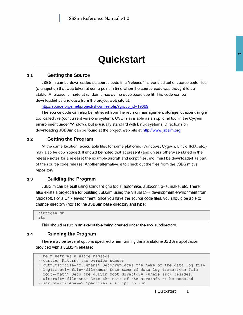
JSBSim can be downloaded as source code in a "release" - a bundled set of source code files (a snapshot) that was taken at some point in time when the source code was thought to be stable. A release is made at random times as the developers see fit. The code can be downloaded as a release from the project web site at:
http://sourceforge.net/project/showfiles.php?group_id=19399 The source code can also be retrieved from the revision management storage location using a
tool called cvs (concurrent versions system). CVS is available as an optional tool in the Cygwin environment under Windows, but is usually standard with Linux systems. Directions on downloading JSBSim can be found at the project web site at http://www.jsbsim.org.
1.2 Getting the Program At the same location, executable files for some platforms (Windows, Cygwin, Linux, IRIX, etc.)
may also be downloaded. It should be noted that at present (and unless otherwise stated in the release notes for a release) the example aircraft and script files, etc. must be downloaded as part of the source code release. Another alternative is to check out the files from the JSBSim cvs repository.
1.3 Building the Program JSBSim can be built using standard gnu tools, automake, autoconf, g++, make, etc. There
also exists a project file for building JSBSim using the Visual C++ development environment from Microsoft. For a Unix environment, once you have the source code files, you should be able to change directory ("cd") to the JSBSim base directory and type:
./autogen.sh make
This should result in an executable being created under the src/ subdirectory.
1.4 Running the Program There may be several options specified when running the standalone JSBSim application
provided with a JSBSim release:
--help Returns a usage message --version Returns the version number --outputlogfile=<filename> Sets/replaces the name of the data log file --logdirectivefile=<filename> Sets name of data log directives file --root=<path> Sets the JSBSim root directory (where src/ resides) --aircraft=<filename> Sets the name of the aircraft to be modeled --script=<filename> Specifies a script to run

JSBSim Reference Manual v1.0
| Quickstart 2
2
--realtime Specifies to run in actual real world time --nice Directs JSBSim to run at low CPU usage --suspend Specifies to suspend the simulation after initialization --initfile=<filename> Specifies an initialization file to use --catalog Directs JSBSim to list all properties for this model --end-time=<time (double)> Specifies the sim end time NOTE: There can be no spaces around the = sign when an option is followed by a filename
If you have built JSBSim from source code there will be an executable under the src/ subdirectory. You can run JSBSim by supplying the name of a script:
src/jsbsim --script=scripts/c1723.xml
You may have simply downloaded the executable. In this case, you should create the scripts/, aircraft/, and engine, subdirectories. You should place aircraft models under the aircraft/ subdirectory, in another subdirectory that has the same name as the aircraft. For instance, if you create a B-2 flight model, you would place that in the aircraft/B2/ subdirectory, and the aircraft flight model name would be called B2.xml.

J
S
JSBSim Refe
Sectio
erence Manu
on 1:
ual v1.0
| Sectio
User'
on One: User’
's Man
’s Manual
nual
3
3
JSBSim Reference Manual v1.0
| Section One: User’s Manual 4
4
1. Overview
1.1 What, exactly, is JSBSim? JSBSim is a collection of program code mostly written in the C++ programming language, but
some C language routines are included. Some of the C++ classes that comprise JSBSim model physical entities such as the atmosphere, a flight control system, or an engine. Some of the classes encapsulate concepts or mathematical constructs such as the equations of motion, a matrix, or a vector. Some classes manage collections of other objects. Taken together, JSBSim takes control inputs, calculates and sums the forces and moments that result from those control inputs and the environment, and advances the state of the vehicle (velocity, orientation, position, etc.) in discrete time steps.
JSBSim has been built and run on a wide variety of platforms such as a PC running Windows or Linux, Apple Macintosh, and even the IRIX operating system from Silicon Graphics. The free GNU g++ compiler easily compiles JSBSim, and other compilers such as those from Borland and Microsoft also work well.
1.2 Who is it for? The JSBSim architecture is meant to be reasonably easy to comprehend, and is designed to
be useful to advanced aerospace engineering students. Due to the ease with which it can be configured, it has also proven to be useful to industry professionals in a number of ways. It has been incorporated into larger, full-featured, flight simulation applications and architectures (such as FlightGear and OpenEaagles), and has been used as a batch simulation tool in industry and academia.
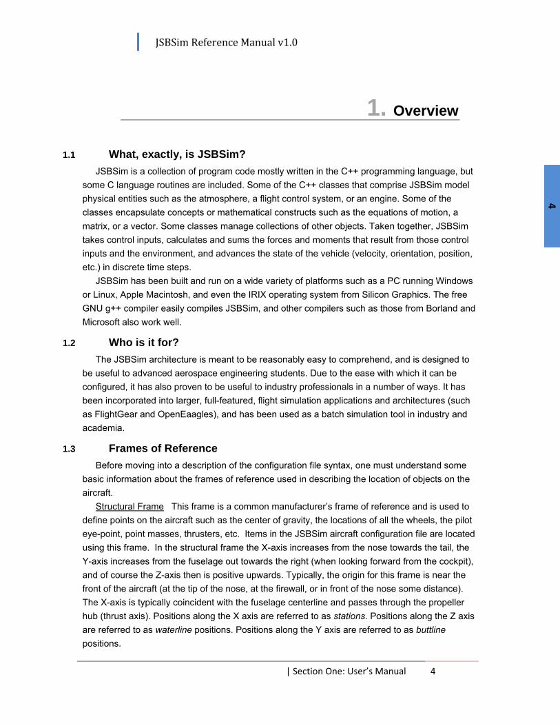
1.3 Frames of Reference Before moving into a description of the configuration file syntax, one must understand some
basic information about the frames of reference used in describing the location of objects on the aircraft.
Structural Frame This frame is a common manufacturer’s frame of reference and is used to define points on the aircraft such as the center of gravity, the locations of all the wheels, the pilot eye-point, point masses, thrusters, etc. Items in the JSBSim aircraft configuration file are located using this frame. In the structural frame the X-axis increases from the nose towards the tail, the Y-axis increases from the fuselage out towards the right (when looking forward from the cockpit), and of course the Z-axis then is positive upwards. Typically, the origin for this frame is near the front of the aircraft (at the tip of the nose, at the firewall, or in front of the nose some distance). The X-axis is typically coincident with the fuselage centerline and passes through the propeller hub (thrust axis). Positions along the X axis are referred to as stations. Positions along the Z axis are referred to as waterline positions. Positions along the Y axis are referred to as buttline positions.

JSBSim Reference Manual v1.0
| Section One: User’s Manual 5
5
Note that the origin can be anywhere for a JSBSim-modeled aircraft, because JSBSim internally only uses the relative distances between the CG and the various objects – not the discrete locations themselves.
Body frame As used in JSBSim, the body frame is similar to the structural frame, but rotated 180 degrees about the Y axis, with the origin coincident with the CG. This is the frame where the aircraft forces and moments are summed and the resulting accelerations are integrated to get velocities.
Stability frame This frame is similar to the body frame, except that the X-axis points into the relative wind vector projected onto the XY plane of symmetry for the aircraft. The Y-axis still points out the right wing, and the Z-axis completes the right-hand system.
Wind frame This frame is similar to the Stability frame, except that the X-axis points directly into the relative wind. The Z-axis is perpendicular to the X-axis, and remains within the aircraft body axis XZ plane (also called the reference plane). The Y-axis completes a right hand coordinate system.
1.4 Units JSBSim uses English units for internal calculations almost exclusively. However, it is possible
to input some parameters in the configuration file using different units. In fact, to avoid confusion, it is recommended that the unit always be specified. Units are specified using the “unit” attribute. For instance, the specification for the wingspan looks like this:
<wingspan unit="FT"> 35.8 </wingspan>
The above statement specifies a wingspan of 35.8 feet. The following statement specifying the wingspan in meters would result in the wingspan being converted to 35.8 feet as it was read in:
<wingspan unit="M"> 10.91 </wingspan>
The two statements for wingspan are effectively equivalent. The following conversions are currently supported [using the abbreviations: “M” – Meters, “FT”
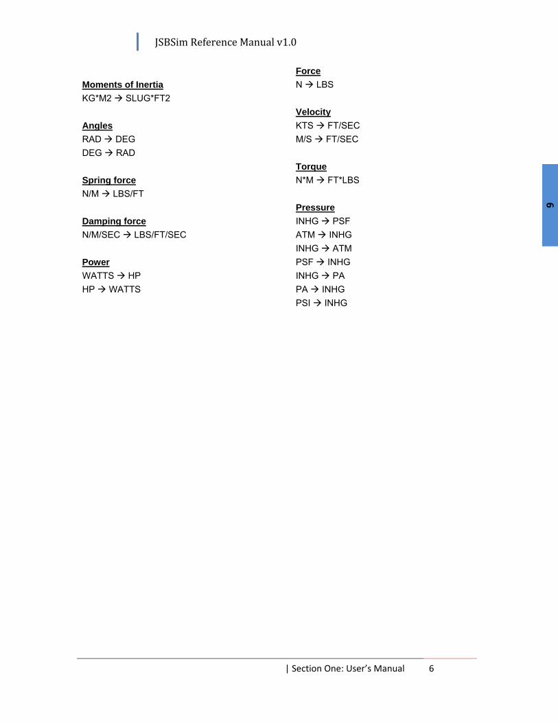
– Feet, “IN” – Inches, “IN3” – Cubic inches, “CC” – Cubic centimeters, “M3” – Cubic meters, “FT3” – Cubic feet, “LTR” – Liter, “M2” – Square meters, “FT2” – Square feet, “LBS” – Pounds, “KG” – Kilogram, “SLUG*FT2” – Slug-ft2, “KG*M2” – Kilogram-meter2, “RAD” – Radian, “DEG” – Degree, “LBS/FT” – pounds per foot, “N/M” – Newtons per meter, “LBS/FT/SEC” – pounds per foot per second, “N/M/SEC” – Newtons per meter per second, “WATTS” – Watts, “HP” – Horsepower, “N” – Newtons, “LBS” – Pounds, “KTS” – Knots, “FT/SEC” – Feet per second, “M/S” – Meters per second, “FT*LBS” – Foot-pounds, “N*M” – Newton-meters, “INHG” – Inches of mercury, “PSF” – Pounds per square foot, “ATM” – atmospheres, “PSI” – Pounds per square inch, “PA” – Pascals]:
Length M FT M IN Area M2 FT2
Volume CC IN3 M3 FT3 LTR->IN3 Mass & Weight KG LBS
JSBSim Reference Manual v1.0
| Section One: User’s Manual 6
6
Moments of Inertia KG*M2 SLUG*FT2 Angles RAD DEG DEG RAD Spring force N/M LBS/FT Damping force N/M/SEC LBS/FT/SEC Power WATTS HP HP WATTS
Force N LBS Velocity KTS FT/SEC M/S FT/SEC Torque N*M FT*LBS Pressure INHG PSF ATM INHG INHG ATM PSF INHG INHG PA PA INHG PSI INHG
JSBSim Reference Manual v1.0
| Section One: User’s Manual 7
7
2. Concepts
2.1 Simulation While the JSBSim user does not need to know some of the finer details of the flight simulator
operation, it can be helpful to understand basically how JSBSim works. Some of the most important concepts are described in this section.
The use of “Properties” permits JSBSim to be a generic simulator, providing a way to interface the various systems with parameters (or variables). Properties are used throughout the configuration files that describe aircraft and engine characteristics.
Obviously, math plays a big part in modeling flight physics. JSBSim makes use of data tables, as flight dynamics characteristics are often stored in tables. Arbitrary algebraic functions can also be set up in JSBSim, allowing broad freedom for describing aerodynamic and flight control characteristics.
2.2 Properties Simulation programs need to manage a large amount of state information. With especially
large programs, the data management task can cause problems:
• Contributors find it harder and harder to master the number of interfaces necessary to make any useful additions to the program, so contributions slow down.
• Runtime configurability becomes increasingly difficult, with different modules using different mechanisms (environment variables, custom specification files, command-line options, etc.).
• The order of initialization of modules is complicated and brittle, since one module's initialization routines might need to set or retrieve state information from an uninitialized module.
• Extensibility through add-on scripts, specification files, etc. is limited to the state information that the program provides, and non-code-writing developers often have to wait too long for the developers to get around to adding a new variable.
The Property Manager system provides a single interface for chosen program state information, and allows the creation of new properties dynamically at run-time. The latter capability is especially important for the JSBSim FCS model because the components that make up the control law definition for an aircraft exist only in a specification file. At runtime, after parsing the component definitions, the components are instantiated, and the property manager creates a property to store the output value of each component.
Properties themselves are like global variables with selectively limited visibility (read or read/write) that are categorized into a hierarchical, tree-like structure that is similar to the structure of a Unix file system. The structure of the property tree includes a root node, sub nodes,
JSBSim Reference Manual v1.0
| Section One: User’s Manual 8
8
(like subdirectories) and end-nodes (properties). Similar to a Unix file system, properties can be referenced relative to the current node, or to the root node. Nodes can be grafted onto other nodes similar to symbolically linking files or directories to other files or directories in a file system. Properties are used throughout JSBSim and FlightGear to refer to specific parameters in program code. Properties can be assigned from the command line, from specification files and scripts, and – in the case of FlightGear – even via a socket interface. References to parameters as properties look like position/h-sl-ft, and aero/qbar-psf.
To illustrate the power of using properties and configuration files, consider the case of a high-performance jet aircraft model. Assume for a moment that a new switch has been added to the control panel for the example aircraft that allows the pilot to override pitch limits in the FCS. For FlightGear, the instrument panel is defined in a configuration file, and the switch is defined there for visual display. A property name is also assigned to the switch definition. Within the flight control portion of the JSBSim aircraft specification file, that same property name assigned to the pitch override switch in the instrument panel definition file can be used to channel the control laws through the desired path as a function of the switch position. No code needs to be touched.
Specific simulation parameters are available both from within JSBSim and in configuration file specifications via properties. As mentioned earlier, properties are the term we use to describe parameters that we can access or set.
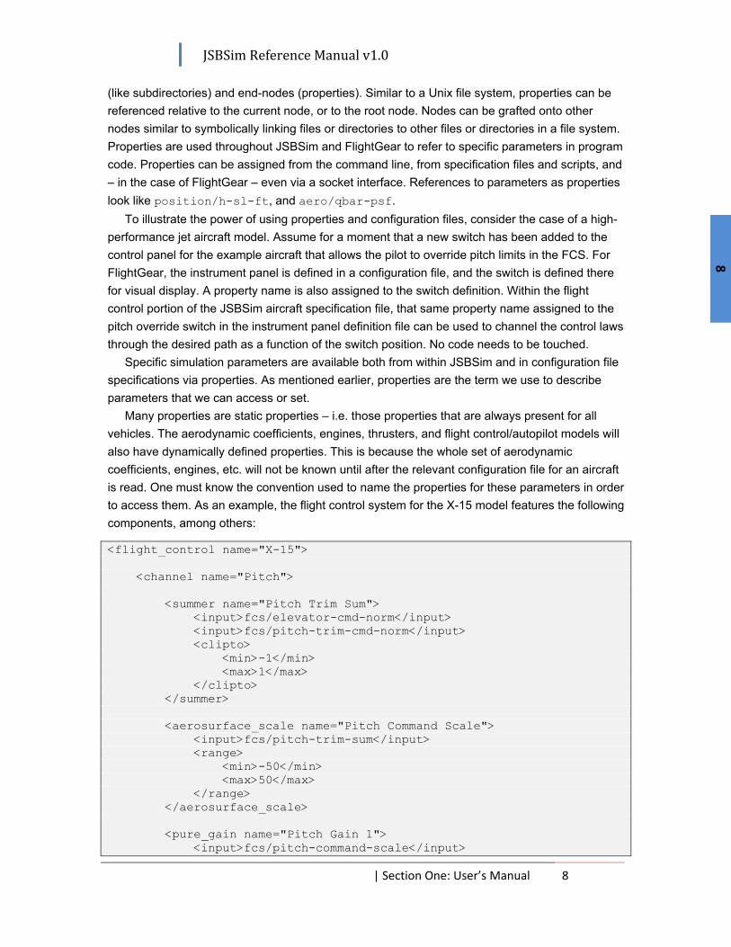
Many properties are static properties – i.e. those properties that are always present for all vehicles. The aerodynamic coefficients, engines, thrusters, and flight control/autopilot models will also have dynamically defined properties. This is because the whole set of aerodynamic coefficients, engines, etc. will not be known until after the relevant configuration file for an aircraft is read. One must know the convention used to name the properties for these parameters in order to access them. As an example, the flight control system for the X-15 model features the following components, among others:
<flight_control name="X-15"> <channel name="Pitch"> <summer name="Pitch Trim Sum"> <input>fcs/elevator-cmd-norm</input> <input>fcs/pitch-trim-cmd-norm</input> <clipto> <min>-1</min> <max>1</max> </clipto> </summer> <aerosurface_scale name="Pitch Command Scale"> <input>fcs/pitch-trim-sum</input> <range> <min>-50</min> <max>50</max> </range> </aerosurface_scale> <pure_gain name="Pitch Gain 1"> <input>fcs/pitch-command-scale</input>

JSBSim Reference Manual v1.0
| Section One: User’s Manual 9
9
<gain>-0.36</gain> </pure_gain>
A close examination of the above series of components reveals a hint as to how the property names are given to components that are defined at runtime. The first component above (“Pitch Trim Sum”) takes input from two places, the known static properties, fcs/elevator-cmd-norm and fcs/pitch-trim-cmd-norm. The next component takes as input the output from the first component. The input property listed for the second component is fcs/pitch-trim-sum. The convention for automatic naming of properties for the flight control system (FCS) and autopilot is that all non-alphanumeric characters in a component name are replaced by hyphens (“-“). This includes spaces and slashes. Additionally, all letters are made lower-case. Continuing with the above case shows that the last component, “Pitch Gain 1”, takes as input the output from the preceding component, “Pitch Command Scale”, which is given the property name (being in the FCS model), fcs/pitch-command-scale.
So, now we have a way to access many parameters inside JSBSim. We know how the FCS is assembled in JSBSim. The same components used in the FCS are also available to build an autopilot, or other system.
2.3 Math 2.3.1 Functions
The function specification in JSBSim is a powerful and versatile resource that allows algebraic functions to be defined in a JSBSim configuration file. The function syntax is similar in concept to MathML (Mathematical Markup Language, www.w3.org/Math/), but it is simpler and more terse.
A function definition consists of an operation, a value, a table, or a property (which evaluates to a value). The currently supported operations are:
• sum (takes n arguments) • difference (takes n arguments) • product (takes n arguments) • quotient (takes 2 arguments) • pow (takes 2 arguments) • exp (takes 2 arguments) • abs (takes n arguments) • sin (takes 1 arguments) • cos (takes 1 arguments) • tan (takes 1 arguments) • asin (takes 1 arguments) • acos (takes 1 arguments) • atan (takes 1 arguments) • atan2 (takes 2 arguments) • min (takes n arguments) • max (takes n arguments) • avg (takes n arguments) • fraction (takes 1 argument)

JSBSim Reference Manual v1.0
| Section One: User’s Manual 10
10
• mod (takes 2 arguments) • random (Gaussian random number, takes no arguments) • integer (takes one argument)
An operation is defined in the configuration file as in the following example:
<sum> <value> 3.14159 </value> <property> velocities/qbar </property> <product> <value> 0.125 </value> <property> metrics/wingarea </property> </product> </sum>
In the example above, the sum element contains three other items. What gets evaluated is written algebraically as:
3.14159 + qbar + (0.125 * wingarea)
A full function definition, such as is used in the aerodynamics section of a configuration file includes the function element, and other elements. It should be noted that there can be only one non-optional (non-documentation) element - that is, one operation element - in the top-level function definition. The <function> element cannot have more than one immediate child operation, property, table, or value element. Almost always, the first operation within the function element will be a product or sum. For example:
<function name="aero/coefficient/Clr"> <description>Roll moment due to yaw rate</description> <product> <property>aero/qbar-area</property> <property>metrics/bw-ft</property> <property>aero/bi2vel</property> <property>velocities/r-aero-rad_sec</property> <table> <independentVar>aero/alpha-rad</independentVar> <tableData> 0.000 0.08 0.094 0.19 </tableData> </table> </product> </function>
The "lowest level" in a function definition is always a value or a property, which cannot itself contain another element. As shown, operations can contain values, properties, tables, or other operations.
Some operations take only a single argument. That argument, however, can be an operation (such as sum) which can contain other items. The point to keep in mind is any such contained operation evaluates to a single value - which is just what the trigonometric functions require (except atan2, which takes two arguments).
Finally, within a function definition, there are some shorthand aliases that can be used for brevity in place of the standard element tags. Properties, values, and tables are normally referred

JSBSim Reference Manual v1.0
| Section One: User’s Manual 11
11
to with the tags, <property>, <value>, and <table>. Within a function definition only, those elements can be referred to with the tags, <p>, <v>, and <t>. Thus, the previous example could be written to look like this:
<function name="aero/coefficient/Clr"> <description>Roll moment due to yaw rate</description> <product> <p> aero/qbar-area </p> <p> metrics/bw-ft </p> <p> aero/bi2vel </p> <p> velocities/r-aero-rad_sec </p> <t> <independentVar> aero/alpha-rad </independentVar> <tableData> 0.000 0.08 0.094 0.19 </tableData> </t> </product> </function>
2.3.2 Tables One, two, or three dimensional lookup tables can be defined in JSBSim for use in
aerodynamics and function definitions. For a single "vector" lookup table, the format is as follows:
<table name="property_name"> <independentVar lookup="row"> property_name </independentVar> <tableData> key_1 value_1 key_2 value_2 ... ... key_n value_n </tableData> </table>
The lookup="row" attribute in the independentVar element is optional in this case; it is assumed that the independentVar is a row variable. A real example is as shown here:
<table> <independentVar lookup="row"> aero/alpha-rad </independentVar> <tableData> -1.57 1.500 -0.26 0.033 0.00 0.025 0.26 0.033 1.57 1.500 </tableData> </table>
The first column in the data table represents the lookup index (or breakpoints, or keys). In this case, the lookup index is aero/alpha-rad (angle of attack in radians). If alpha is 0.26 radians, the value returned from the lookup table would be 0.033.
The definition for a 2D table, is as follows:
<table name="property_name">

JSBSim Reference Manual v1.0
| Section One: User’s Manual 12
12
<independentVar lookup="row"> property_name </independentVar> <independentVar lookup="column"> property_name </independentVar> <tableData> col_1_key col_2_key ... col_n_key row_1_key col_1_data col_2_data ... col_n_data row_2_key ... ... ... ... ... ... ... ... ... row_n_key ... ... ... ... </tableData> </table>
The data is in a gridded format. A real example is as shown below. Alpha in radians is the row lookup (alpha breakpoints are arranged in the first column) and flap position in degrees is split up in columns for deflections of 0, 10, 20, and 30 degrees):
<table> <independentVar lookup="row">aero/alpha-rad</independentVar> <independentVar lookup="column">fcs/flap-pos-deg</independentVar> <tableData> 0.0 10.0 20.0 30.0 -0.0523599 8.96747e-05 0.00231942 0.0059252 0.00835082 -0.0349066 0.000313268 0.00567451 0.0108461 0.0140545 -0.0174533 0.00201318 0.0105059 0.0172432 0.0212346 0.0 0.0051894 0.0168137 0.0251167 0.0298909 0.0174533 0.00993967 0.0247521 0.0346492 0.0402205 0.0349066 0.0162201 0.0342207 0.0457119 0.0520802 0.0523599 0.0240308 0.0452195 0.0583047 0.0654701 0.0698132 0.0333717 0.0577485 0.0724278 0.0803902 0.0872664 0.0442427 0.0718077 0.088081 0.0968405 </tableData> </table>
The definition for a 3D table in a coefficient would be (for example):
<table name="property_name"> <independentVar lookup="row"> property_name </independentVar> <independentVar lookup="column"> property_name </independentVar> <tableData breakpoint="table_1_key"> col_1_key col_2_key ... col_n_key row_1_key col_1_data col_2_data ... col_n_data row_2_key ... ... ... ... ... ... ... ... ... row_n_key ... ... ... ... </tableData> <tableData breakpoint="table_2_key"> col_1_key col_2_key ... col_n_key row_1_key col_1_data col_2_data ... col_n_data row_2_key ... ... ... ... ... ... ... ... ... row_n_key ... ... ... ... </tableData> ... <tableData breakpoint="table_n_key"> col_1_key col_2_key ... col_n_key row_1_key col_1_data col_2_data ... col_n_data row_2_key ... ... ... ... ... ... ... ... ...

JSBSim Reference Manual v1.0
| Section One: User’s Manual 13
13
row_n_key ... ... ... ... </tableData> </table>
[Note the "breakpoint" attribute in the tableData element, above.] Here's an example:
<table> <independentVar lookup="row">fcs/row-value</independentVar> <independentVar lookup="column">fcs/column-value</independentVar> <independentVar lookup="table">fcs/table-value</independentVar> <tableData breakPoint="-1.0"> -1.0 1.0 0.0 1.0000 2.0000 1.0 3.0000 4.0000 </tableData> <tableData breakPoint="0.0000"> 0.0 10.0 2.0 1.0000 2.0000 3.0 3.0000 4.0000 </tableData> <tableData breakPoint="1.0"> 0.0 10.0 20.0 2.0 1.0000 2.0000 3.0000 3.0 4.0000 5.0000 6.0000 10.0 7.0000 8.0000 9.0000 </tableData> </table>
Note that table values are interpolated linearly, and no extrapolation is done at the table limits – the highest value a table will return is the highest value that is defined.
2.4 Forces and Moments 2.4.1 Aerodynamics
There are several ways to model the aerodynamic forces and moments (torques) that act on an aircraft. JSBSim started out by using the coefficient buildup method. In the coefficient buildup method, the lift force (for instance) is determined by summing all of the contributions to lift. The contributions differ depending on the aircraft and the fidelity of the model, but contributions to lift can include those from:
• Wing • Elevator • Flaps
Aerodynamic coefficients are numbers which, when multiplied by certain other values (such as dynamic pressure and wing area), result in a force or moment. The coefficients can be taken from flight test reports or textbooks, or they can be calculated using software (such as Digital DATCOM or other commercially available programs) or by hand calculations.
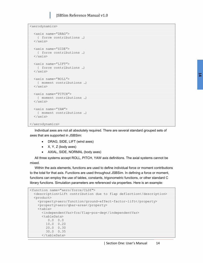
Eventually, JSBSim added support for aerodynamic properties specified as functions. Within the <aerodynamics> section of a configuration file there are six subsections representing the 3 force and 3 moment axes (for a total of six degrees of freedom). The basic layout of the aerodynamics section is as follows:
JSBSim Reference Manual v1.0
| Section One: User’s Manual 14
14
<aerodynamics> <axis name=”DRAG”> force contributions … </axis> <axis name=”SIDE”> force contributions … </axis> <axis name=”LIFT”> force contributions … </axis> <axis name=”ROLL”> moment contributions … </axis> <axis name=”PITCH”> moment contributions … </axis> <axis name=”YAW”> moment contributions … </axis> </aerodynamics>
Individual axes are not all absolutely required. There are several standard grouped sets of axes that are supported in JSBSim:
• DRAG, SIDE, LIFT (wind axes) • X, Y, Z (body axes) • AXIAL, SIDE, NORMAL (body axes)
All three systems accept ROLL, PITCH, YAW axis definitions. The axial systems cannot be mixed.
Within the axis elements, functions are used to define individual force or moment contributions to the total for that axis. Functions are used throughout JSBSim. In defining a force or moment, functions can employ the use of tables, constants, trigonometric functions, or other standard C library functions. Simulation parameters are referenced via properties. Here is an example:
<function name="aero/force/CLDf"> <description>Lift contribution due to flap deflection</description> <product> <property>aero/function/ground-effect-factor-lift</property> <property>aero/qbar-area</property> <table> <independentVar>fcs/flap-pos-deg</independentVar> <tableData> 0.0 0.0 10.0 0.20 20.0 0.30 30.0 0.35 </tableData>

JSBSim Reference Manual v1.0
| Section One: User’s Manual 15
15
</table> </product> </function>
In this case, a description in words of what the above does is as follows: CLDf (the contribution of lift due to flap deflection) is the product of the ground-effect-factor-lift, qbar-area, and the value determined by the table, which is indexed as a function of flap position in degrees.
All of the functions in an <axis> section are summed and applied to the aircraft in the appropriate manner. There is some flexibility in this format, though. Functions that are specified outside of any <axis> section are created and calculated, but they do not specifically contribute to any force or moment total by themselves. However, they can be referenced by other functions that are in an <axis> section. This technique allows calculations that might be applied to several individual functions to be performed once and used several times. The technique can be taken even further, with actual aerodynamic coefficients being calculated outside of an <axis> definition, with the coefficients subsequently being multiplied within function definitions by the various factors (properties) that turn them into forces and moments inside an <axis> definition.
As an example, let’s examine the lift force due to angle of attack (alpha). We know that increasing the angle of attack increases lift – up to a point. Lift force is traditionally defined as the product of dynamic pressure (qbar), wing area (Sw), and lift coefficient (CL). In this case, the lift coefficient is determined via a lookup table, using alpha as an index into the table:
<function name="aero/coefficient/CLalpha"> <description> Lift_due_to_alpha </description> <product> <property> aero/qbar-psf </property> <property> metrics/Sw-sqft </property> <table name=”CL”> <independentVar lookup="row"> aero/alpha-rad </independentVar> <tableData> -0.20 -0.720 0.00 0.240 0.22 1.300 0.60 0.664 </tableData> </table> </product> </function>
The above function results in “CLalpha” being calculated many times per second as JSBSim executes. The value of the function is the product of qbar, wing area, and lift coefficient as determined by the lookup table. For instance, if alpha (in radians) is 0 degrees, the lift coefficient is 0.240.
So, for the aircraft we are modeling, where do we get this information about the lift coefficient – or any other aerodynamic data? An early task in modeling any aircraft is to collect the aircraft characteristics information – a sort of “data farming” effort. One can begin with a search using the NASA Technical Report Server search engine at: http://ntrs.nasa.gov. For instance, a search phrase of “Beech 99” returned several documents, and one was available as a PDF file:
Stability and control derivative estimates obtained from flight data for the Beech 99 aircraft, Tanner, R. R.; Montgomery, T. D.

JSBSim Reference Manual v1.0
| Section One: User’s Manual 16
16
Lateral-directional and longitudinal stability and control derivatives were determined from flight data by using a maximum likelihood estimator for the Beech 99 airplane. Data were obtained with the aircraft in the cruise configuration and with one-third flap deflection. The estimated derivatives show good agreement with the predictions of the manufacturer.
Next, one might search for an FAA Type Certificate Data Sheet (TCDS) at: http://www.airweb.faa.gov/Regulatory_and_Guidance_Library/rgMakeModel.nsf/ A careful search led to “TYPE CERTIFICATE DATA SHEET NO. A14CE” for the Beech 99
aircraft. Documents such as these can be helpful in crafting an aircraft aerodynamic model. If you are
unable to find stability and aerodynamic information about the aircraft you are interested in, try finding a comparable aircraft. For instance, the CV-880, B747, and C-5 all have data published in Aircraft Handling Qualities Data, by Heffley and Jewell.
First of all, the NASA Beech 99 Technical Memo mentioned above contains specific information about the aerodynamic qualities of the aircraft. Let’s look at how to begin creating a JSBSim aerodynamics specification for a specific aircraft.
As mentioned, JSBSim uses the coefficient buildup method for calculating aerodynamic forces and moments on an aircraft. We have a nice report for the Beech 99 showing both the manufacturer’s estimates and flight test data for the aerodynamic quantities:
Longitudinal coefficients (i.e. xz-plane symmetric coefficients, lift, pitch, drag)
(1) 0NeNNN CCCC
e++= δα
δα
(2) 02 memmmm CC
VcqCCC
eq+++= δα δα
(3) 20 LDD KCCC +=
Lateral coefficients (i.e. side force, roll, yaw)
(4) 0YrYaYYY CCCCC
ra+++= δδβ δδβ
(5) 022 lrlalllll CCC
VrbC
VpbCCC
rarp+++++= δδβ δδβ
(6) 022 nrnannnnn CCC
VrbC
VpbCCC
rarp+++++= δδβ δδβ
The above equations are for (in order), normal force coefficient, pitch moment coefficient, drag coefficient, side force coefficient, rolling moment coefficient, and yaw moment coefficient. There is no lift coefficient specified. For low alpha, the normal and lift coefficients are very close.
The manufacturer’s estimates for the aerodynamic force and moment components are as follows:
(7) cL TC ⋅+= 151.0096.0α
(per degree; no flaps)
(8) cL TC ⋅+= 151.0101.0α
(per degree; 1/3 flaps)
(9) 20625.00275.0 LD CC ⋅+=
JSBSim Reference Manual v1.0
| Section One: User’s Manual 17
17
(10) cm TC ⋅+= 010.0010.04/1,α
(per degree)
(11) cm TCe
⋅−−= 032.0034.0δ (per degree)
(12) 1.43−=α&mC (per radian)
(13) 40.3−=qmC (per radian)
(14) cn TC ⋅−= 0015.0014.0β
(per degree)
(15) 0023.0−=βl
C (per degree)
(16) 010.0−=βYC (per degree)
(17) 0014.0−=rnC δ (per degree)
(18) αδ ⋅−= 000022.000017.0rlC (per degree)
(19) 0026.0=rYC δ (per radian)
(20) α⋅−−= 197.020.0rnC (per radian)
(21) α⋅+= 623.005.0rl
C (per radian)
(22) 394.0=rYC (per radian)
(23) α⋅−= 762.00079.0pnC (per radian)
(24) 515.0−=pl
C (per radian)
(25) α⋅−−= 385.0199.0pYC (per radian)
(26) 0027.0=alC δ (per degree)
(27) 0015.0−=anC δ (per degree)
The subscripts p, q, r, refer to rates about the x, y, z, axes; δx (where x is a, r, e) refers to the deflection of the aileron, rudder, or elevator, respectively; l, m, n, refer to moments about the x, y, z, axes; α, β, refer to angle of attack and angle of sideslip; L, D, and Y, refer to lift, drag, and side force. Tc refers to thrust coefficient, and is defined as follows:
(28) Sq
ThrustTc =
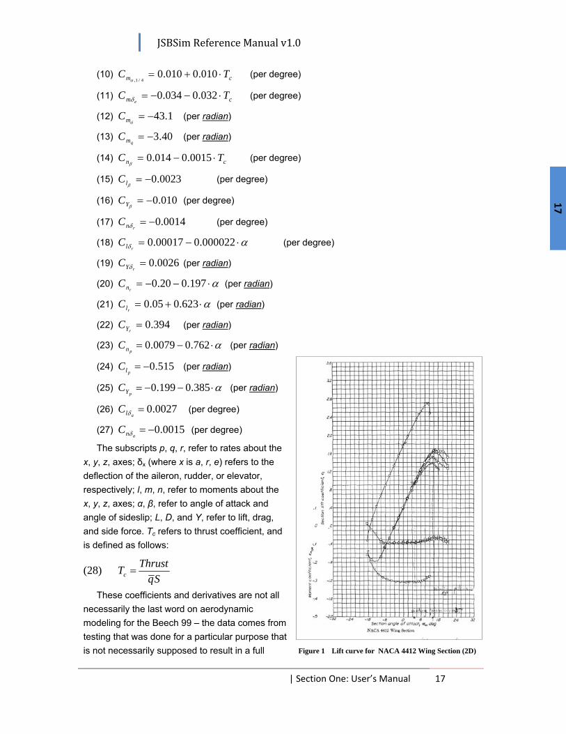
These coefficients and derivatives are not all necessarily the last word on aerodynamic modeling for the Beech 99 – the data comes from testing that was done for a particular purpose that is not necessarily supposed to result in a full Figure 1 Lift curve for NACA 4412 Wing Section (2D)

JSBSim Reference Manual v1.0
| Section One: User’s Manual 18
18
aerodynamic database for simulation modeling. So, we are left with data obtained within a fairly narrow flight envelope. We can look at the coefficient and derivative data and make adjustments on a one-by-one basis. But, not only are there adjustments that can be made to the set of coefficients, but additional ones that can be added in.
Let’s consider CLα first. The symbol CLα is shorthand for δCL/δα, or the change in lift coefficient with a change in alpha. This is just the slope of the lift coefficient curve (see Figure 1 for an example). The lift curve slope for an ideal 2D airfoil section is 2π (per radian). For a cambered airfoil, the lift curve does not pass through zero – that is, there is an inherent lift to the airfoil even at zero angle of attack. Furthermore, a real wing (i.e. not a 2D airfoil section) is not as efficient as an airfoil, and the slope of the lift curve will be somewhat less than 2π. Additionally, a real wing will eventually stall at a particular angle of attack, perhaps around 12-16 degrees. The information given in the Beech 99 report is valuable; however, some adjustments will have to be made to account for stalling. The value of CLα defines a slope – a line that goes on forever! Knowing that the lift attributable to alpha is complex – it’s not a straight line – we might instead consider creating a lookup table or function that includes the behavior at stall. Unfortunately, little or no information is given to us about stall in the document, but some searching suggests 73 kts (123 ft/sec) as the stall speed. Also, what about the post-stall behavior? Modeling post-stall and very high alpha regimes is effectively beyond the scope of this discussion, but suffice it so say we would like to provide plausible behavior in all regimes where possible. In this case, we can look to a study done by Sandia Labs some years ago. The study resulted in data being collected that showed the lift coefficient as it varied with angle of attack for symmetric airfoils of varying
thickness, across the entire alpha range of 0 to 180 degrees. Figure 2 shows the lift coefficient for an airfoil for a full range of alpha. The thickness of the airfoil represented by the data in Figure 2 is 12%. The blended-airfoil wing used on the Beech 99 is 18% thick at the root and 12% thick at the tip. We will assert that we can use the data for a 15% thick airfoil as representative of the average characteristic of the wing.

JSBSim Reference Manual v1.0
| Section One: User’s Manual 19
19
Not including thrust effects at the moment, the lift coefficient of the wing can be written as:
Lift coefficient = 0.939 * table value + (0.25 * Df * 0.017) + 0.3
The lift force is just the above coefficient multiplied by qbar and area:
Lift force = qbar * wingarea * Lift_coefficient
The equation was developed by asserting that:
• the effect of camber on the airfoil data effectively adds 0.3 to the lift coefficient, • for a 3-D wing the curve must be scaled (0.939), • adding a flap setting in degrees (multiplied by 0.017 to convert it to a radian
measurement) multiplied by 0.25 gives the increase in lift coefficient from flaps
The JSBSim-ML representation of the lift of a wing using the 15% thick Sandia data and information from “Theory of Wing Sections”, NACA wing data, etc. is shown as:
<function name="aero/force/CLalpha"> <description> Lift force due to alpha </description> <product> <property>aero/qbar-psf</property> <property>metrics/Sw-sqft</property> <sum name=”aero/coefficient/CLalpha”> <value> 0.3 </value> <!-- Lift curve slope camber shift --> <product> <value> 0.25 </value> <!-- flap setting curve shift --> <property> fcs/flap-pos-deg </property> <value> 0.017 </value> <!-- convert degrees to radians --> </product> <product> <value> 0.939583333 </value> <!-- Lift curve scaling value --> <table name=”aero/coefficient/Clalpha”> <independentVar lookup="row">aero/alpha-deg</independentVar> <tableData> -180 0.0000 -170 0.8500 -160 0.6350 -150 0.7700 -140 0.9800 -130 0.8500 -120 0.6700 -110 0.4500 -100 0.1850 ... ... 60 0.8750 70 0.6300 80 0.3650 90 0.0900 100 -0.1850 110 -0.4500 120 -0.6700 130 -0.8500 140 -0.9800 150 -0.7700 160 -0.6350 170 -0.8500

JSBSim Reference Manual v1.0
| Section One: User’s Manual 20
20
Wingspan 45.9 feet (13.98 meters)
Horizontal tail span 22.38 feet (6.82 meters)Tail area 100 feet2 (9.29 meters2)
MAC 4.63 feet (1.41 meters)Aspect Ratio 5.0
Sweep 17°
Dihedral 7°
2 Hartzell HC-B3TN-3 or HC-B3TN-3B hubs with Hartzell T10173E-8 or T10173B-8 blades. Diameter: 93-3/8 in. Pitch settings at 30 in. sta.: Reversing propeller: Reverse - 11° Feather - 87°
Flight idle propeller low pitch stop is set so that at 2000 r.p.m., torque shall be an indicated 600 +60 ft.-lb. corrected for sea level standard day. Secondary flight idle stop shall be 210 +40 propeller r.p.m. higher than flight idle stop with a gas generator speed of 70 percent.
Fuselage/Propeller clearance 3 inches (0.076 meters)
Engine thrust lines and wheelbase span 13 feet (3.96 meters) Flap total Area 37.8 ft2 (3.51 m2) Flap span (each) 12.4 ft (3.78 m) Flap chord 1.5 feet (0.46 m)
Beechcraft B99Model A99A Airliner
Engines: Pratt & Whitney PT6A-27, Shaft HP 680, Equiv. Shaft HP 715, Jet thrust 76 lbs., Max. allowable TIT 1337° F (725° C). Propeller shaft speed 2100 rpm. Burns JP-4, JP-5, JP-8, Jet A, Jet A-1, Jet B
Maximum operating speed: 260 mph (226 kts, @ 15.5kft, for 15.5kft to 25kft decrease 4 kts per 1kft) Maneuvering speed: 195 mph (169 kts) Flaps extend speed: 161 mph (140 kts) Landing gear extend: 180 mph (156 kts) Landing gear operating: 150 mph (130 kts)
Flaps Maximum 43° Aileron up 18°, down 15° Elevator up 12°, down 15° Stabilizer up 4.25°, down 3.5° Rudder right 26°, left 20°
Datum: 190” fwd of main spar
Weight Empty equipped 5777 lbs. (2620 kg) Full Fuel Max takeoff 10,900 lbs. (4944 kg) CG @ +179 to +195 in. (gear extended), 26% MAC Ixx 12,464.8 slug-ft2 (16,900 kg-m2) Iyy 17,627 slug-ft2 (23,900 kg-m2) Izz 28,691 slug-ft2 (38,900 kg-m2)
Wing area 279.97 ft2 (26.01 meters2) Wing chord (MAC) 6.5 feet (1.98 meters) Aspect Ratio 7.54 Dihedral 6.8 degrees Wing root airfoil NACA 23018 Wing tip airfoil NACA 23012
Elevator Area 26.4 ft2 (2.45 m2) MAC 0.39
Vertical tailArea 44.9 ft2 (4.17 m2)Span 7.6 ft (2.32 m)MAC 6.3 ft (1.9 m) AR 1.29 Sweep 19.5°
18 feet (5.48 meters)
Engine thrust offset 2°
Height 14.4 feet (4.38 m) Rudder
Area 12 ft2 (1.12 m2)MAC 0.55
Aileron total area 13.9 ft2 (1.29 m2) Aileron span (each) 7.9 ft (2.4 m) Aileron chord 0.9 ft (0.28 m)
180 0.0000 </tableData> </table> </product> </sum> </product> </function>
This specification should produce a fairly smoothly changing lift force in a wide range of conditions. Note that this is a force calculation – the lift coefficient has been multiplied with qbar and the area of the wing.
This function defining the lift force on the wing due to angle of attack is but one contribution to the total lift force on the aircraft. When the elevator is moved, it also changes the lift force of the tail, which results in a pitch moment on the aircraft – the main purpose of the elevator – but the change in lift force must be taken into account in the total lift force calculation.
Developing an accurate aerodynamic model of an aircraft is an art form in itself, and crafting more accurate and detailed aerodynamic models can involve great expense and effort using wind tunnels and computational facilities. But the first step is to gather as much information as is possible for the vehicle being modeled.
2.4.2 Propulsion Several different engine types are
modeled in JSBSim,
• Piston • Rocket • Turbine • Turboprop • Electric
They are generic models, because the characteristics that define a specific engine must be entered in an engine configuration file. Any number of engines (the same or different) can be included in an aircraft configuration file by referring to the name of the engine file, and specifying placement information in the aircraft configuration file in the <engine> element. At runtime, the

JSBSim Reference Manual v1.0
| Section One: User’s Manual 21
21
forces and moments generated by each engine are calculated and summed together.
2.4.3 Ground reactions 2.4.4 External reactions 2.5 Flight Control and Systems modeling 2.5.1 System components
Flight control laws, stability augmentation systems, autopilots, and arbitrary aircraft systems (avionics, electrical systems, etc.) can be modeled in JSBSim by creating chains of individual control components. A suite of configurable components is available in JSBSim that includes gains, filters, switches, etc. An aircraft system is specified as a string of components within the <channel> element of a <system>, <autopilot>, or <flight_control> specification in the aircraft configuration file. Groupings of components which perform a related task are placed in a <channel> element. For example,
<autopilot name=”C172X Autopilot”> <!-- Wing leveler --> <channel name="Roll wing leveler"> <pid name="fcs/roll-ap-error-pid"> <input>attitude/phi-rad</input> <kp> 1.0 </kp> <ki> 0.01</ki> <kd> 0.1 </kd> </pid> <switch name="fcs/roll-ap-autoswitch"> <default value="0.0"/> <test value="fcs/roll-ap-error-pid"> ap/attitude_hold == 1 </test> </switch> <pure_gain name="fcs/roll-ap-aileron-command-normalizer"> <input>fcs/roll-ap-autoswitch</input> <gain>-1</gain> </pure_gain> </channel> <channel name=”Pitch attitude hold”> … components … </channel> … additional channels … </autopilot>
A component will calculate its own output, and that value will be passed to another component later on.
Historically, the flight control section was the first section to be implemented in JSBSim. Later,

JSBSim Reference Manual v1.0
| Section One: User’s Manual 22
22
the autopilot section was added, and then the system section, to support any arbitrary system. Note that it is possible that the system section may replace the autopilot and flight control sections. There can be any number of system sections. Also, any of the three sections may include a reference to a filename, loading the system definition from a system file rather than defining the system inline by specifying a value for the file attribute. For example:
<autopilot file="c172ap"/>
The file “c172ap.xml” will be searched for in the same directory as the aircraft file is found in. Common system files are searched for in the systems/ directory.
Each of the system components is described in Section, 4.1.9.
2.5.2 Automatic Flight in JSBSim One long-time goal of JSBSim has been to support automatic, scripted flights. Scripted flights
refer to the ability of JSBSim to run in a standalone mode (apart from visuals) and fly in a stable manner to various targets, be they altitude and heading, or latitude and longitude, etc. This is a useful feature for many reasons, among them being regression testing of JSBSim, aircraft flight model performance testing, and control system development.
Some of the features that make capability possible include the incorporation of switch and function components, sensors, and autopilot-related properties.
In implementing automatic flight in JSBSim, several files are involved:
• A script file directs the aircraft to turn on its engine, advance the throttle, and fly to a target heading, altitude, and/or velocity. The script file and processing capability takes the role of guidance.
• The aircraft configuration file defines the aircraft properties – including the flight control system, and the interface to the autopilot (or it could even include the autopilot itself).
• The autopilot definition file (if separate).
The job of an autopilot is to attain a state such as wings level, or a heading, or an altitude, and hold it. Designing an autopilot for an aircraft is a science in itself – we will only gloss over the design aspect, paying the most attention on how to implement one and use it in JSBSim.
As an example, we can set out to build a wing-leveler autopilot. Wings-level is by definition a roll angle of zero (phi=0). Many forces will tend to disrupt a state of wings-level, such as engine torque, atmospheric turbulence, fuel slosh, etc. To get to a phi of zero (assuming phi is initially non-zero) we will need to attain a non-zero phi rate, which drives us towards wings-level. To get the phi rate, we will need to attain a phi acceleration, which is controlled by aileron deflection.
One possibility is to simply command the ailerons based on the roll angle. This is called proportional control, because the output is simply the input multiplied by a value – the output is proportional to the input. The autopilot aileron command is sent to the main flight control system and summed in to the aileron command channel. There are a couple of nuances to this autopilot arrangement, however. For instance, it is always on. A better arrangement is shown on the next page.

JSBSim Reference Manual v1.0
| Section One: User’s Manual 23
23
Roll A/P ON Also, the min, max, and K values must be chosen properly. As an example, we set up JSBSim
to run with this autopilot and see what the response is. Here is the autopilot we use, in JSBSim format:
<channel name="AP Roll Wing Leveler"> <pure_gain name="Roll AP Wing Leveler"> <input> attitude/phi-rad </input> <gain>2.0</gain> <clipto> <min>-0.255</min> <max>0.255</max> </clipto> </pure_gain> <switch name="Roll AP Autoswitch"> <default value="0.0"/> <test logic="AND" value="fcs/roll-ap-wing-leveler"> ap/attitude_hold == 1 </test> </switch> <pure_gain name="Roll AP Aileron Command Normalizer"> <input>fcs/roll-ap-autoswitch</input> <gain>-1</gain> </pure_gain> </channel>
There are a couple of points to make about the above listing. First, for the Roll A/P Wing Leveler component, there could be a “<gain> 1 </gain>” line in the definition, however, gain is 1 by default for the pure gain component. Second, the output of the control is limited to ± 0.255 radians (15 degrees). This is about all the ailerons can produce anyhow. The ap/attitude_hold property in the Roll A/P Autoswitch is functionally the Roll A/P ON switch shown in the previous diagram.
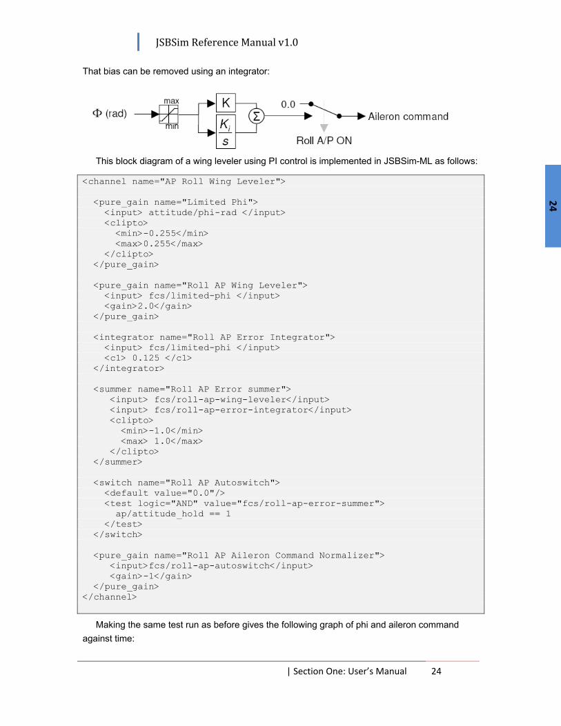
It is seen in the graph that once the transient damps out there is a bias in the roll angle (phi).
JSBSim Reference Manual v1.0
| Section One: User’s Manual 24
24
That bias can be removed using an integrator:
This block diagram of a wing leveler using PI control is implemented in JSBSim-ML as follows:
<channel name="AP Roll Wing Leveler"> <pure_gain name="Limited Phi"> <input> attitude/phi-rad </input> <clipto> <min>-0.255</min> <max>0.255</max> </clipto> </pure_gain> <pure_gain name="Roll AP Wing Leveler"> <input> fcs/limited-phi </input> <gain>2.0</gain> </pure_gain> <integrator name="Roll AP Error Integrator"> <input> fcs/limited-phi </input> <c1> 0.125 </c1> </integrator> <summer name="Roll AP Error summer"> <input> fcs/roll-ap-wing-leveler</input> <input> fcs/roll-ap-error-integrator</input> <clipto> <min>-1.0</min> <max> 1.0</max> </clipto> </summer> <switch name="Roll AP Autoswitch"> <default value="0.0"/> <test logic="AND" value="fcs/roll-ap-error-summer"> ap/attitude_hold == 1 </test> </switch> <pure_gain name="Roll AP Aileron Command Normalizer"> <input>fcs/roll-ap-autoswitch</input> <gain>-1</gain> </pure_gain> </channel>
Making the same test run as before gives the following graph of phi and aileron command against time:

JSBSim Reference Manual v1.0
| Section One: User’s Manual 25
25
The roll angle is seen in the above graph to settle out, now, to wings level. There is, however,
a good degree of overshoot initially. This is where the tweaking comes into play. One can vary the relative contributions of the proportional and integral parts of the control command to achieve different results. However, in turbulence, for instance, the response may be different than what is expected, perhaps even unstable. Often, it is expected that the autopilot will be turned off in bad weather.
There is yet another kind of control action we can use, called derivative control. Derivative control action produces a control command that is proportional to the rate of change of the error. In our wing leveler case – where we seek zero roll angle – the rate of change of the error is simply the roll rate, “p”. If that parameter is summed in, the resulting controller is a PID controller (Proportional-Integral-Derivative).
If we play around with the gains we can tailor the wing leveler to give the best response. The final control system block diagram for the wing leveler is:
This is represented in JSBSim as follows:
<channel name="AP Roll Wing Leveler"> <pure_gain name="Limited Phi"> <input> attitude/phi-rad </input> <clipto> <min>-0.255</min> <max>0.255</max> </clipto> </pure_gain> <pure_gain name="Roll AP Wing Leveler"> <input> fcs/limited-phi </input> <gain>2.0</gain> </pure_gain>

JSBSim Reference Manual v1.0
| Section One: User’s Manual 26
26
<integrator name="Roll AP Error Integrator"> <input> fcs/limited-phi </input> <c1> 0.125 </c1> </integrator> <summer name="Roll AP Error summer"> <input> velocities/p-rad_sec</input> <input> fcs/roll-ap-wing-leveler</input> <input> fcs/roll-ap-error-integrator</input> <clipto> <min>-1.0</min> <max> 1.0</max> </clipto> </summer> <switch name="Roll AP Autoswitch"> <default value="0.0"/> <test logic="AND" value="fcs/roll-ap-error-summer"> ap/attitude_hold == 1 </test> </switch> <pure_gain name="Roll AP Aileron Command Normalizer"> <input>fcs/roll-ap-autoswitch</input> <gain>-1</gain> </pure_gain> </channel>
We see now that our wing leveler controller is performing as desired.
JSBSim Reference Manual v1.0
| Section One: User’s Manual 27
27
3. Authoring Configuration Files
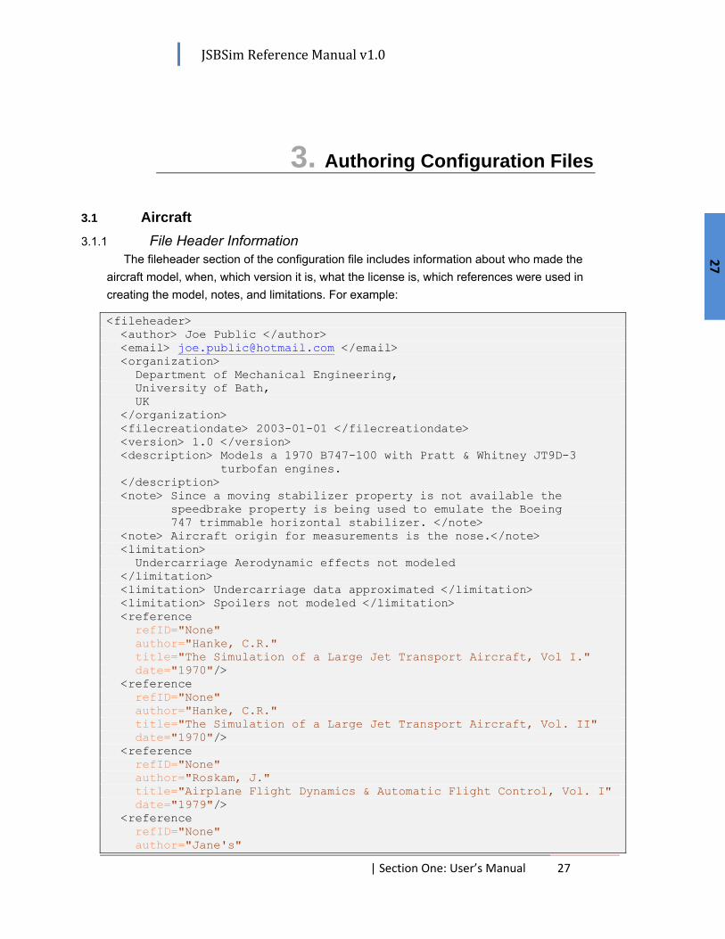
3.1 Aircraft 3.1.1 File Header Information
The fileheader section of the configuration file includes information about who made the aircraft model, when, which version it is, what the license is, which references were used in creating the model, notes, and limitations. For example:
<fileheader> <author> Joe Public </author> <email> [email protected] </email> <organization> Department of Mechanical Engineering, University of Bath, UK </organization> <filecreationdate> 2003-01-01 </filecreationdate> <version> 1.0 </version> <description> Models a 1970 B747-100 with Pratt & Whitney JT9D-3 turbofan engines. </description> <note> Since a moving stabilizer property is not available the speedbrake property is being used to emulate the Boeing 747 trimmable horizontal stabilizer. </note> <note> Aircraft origin for measurements is the nose.</note> <limitation> Undercarriage Aerodynamic effects not modeled </limitation> <limitation> Undercarriage data approximated </limitation> <limitation> Spoilers not modeled </limitation> <reference refID="None" author="Hanke, C.R." title="The Simulation of a Large Jet Transport Aircraft, Vol I." date="1970"/> <reference refID="None" author="Hanke, C.R." title="The Simulation of a Large Jet Transport Aircraft, Vol. II" date="1970"/> <reference refID="None" author="Roskam, J." title="Airplane Flight Dynamics & Automatic Flight Control, Vol. I" date="1979"/> <reference refID="None" author="Jane's"

JSBSim Reference Manual v1.0
| Section One: User’s Manual 28
28
title="Jane's All The World's Aircraft 1980-1981" date="1981"/> </fileheader>
3.1.2 Metrics The metrics section of the configuration file defines the characteristic measurements of the
vehicle and the locations of key points. For example:
<wingarea unit="FT2"> 174.0 </wingarea> <wingspan unit="FT"> 35.8 </wingspan> <chord unit="FT"> 4.9 </chord> <htailarea unit="FT2"> 21.9 </htailarea> <htailarm unit="FT"> 15.7 </htailarm> <vtailarea unit="FT2"> 16.5 </vtailarea> <vtailarm unit="FT"> 15.7 </vtailarm> <location name="AERORP" unit="IN"> <x> 43.2 </x> <y> 0.0 </y> <z> 59.4 </z> </location> <location name="EYEPOINT" unit="IN"> <x> 37.0 </x> <y> 0.0 </y> <z> 48.0 </z> </location> <location name="VRP" unit="IN"> <x> 42.6 </x> <y> 0.0 </y> <z> 38.5 </z> </location>
The Visual Reference Point (VRP) is not really important to flight dynamics. If you are using JSBSim within a larger simulation framework that includes a visual system, then it matters. When placing a 3D model in the scene, you might ask yourself the question: given that my 3D model can have it's origin at any arbitrary spot, how do I make sure I am placing the aircraft exactly where the flight model specifies that it should be? When you are flying and are at high altitude, the question might not seem all that critical. However, when you are on the ground, if model placement is not correct, then the model may be seen to "hover", or to be embedded in the ground. Or, when you rotate at takeoff, you may rotate into the ground.
So, correct placement is important. The flight model calculates motion about the aircraft CG, and reports the current position of
the CG. The CG might be thought of as a good "origin" for the 3D model, but the CG moves as fuel burns off.
The VRP is simply an agreed upon point on the aircraft, for which the flight model will provide the latitude/longitude/altitude. The VRP is defined in JSBSim in the same structural frame in which the landing gear, empty weight CG, etc. are defined. By convention, the nose of the aircraft is usually taken to be the point to be reported as the VRP.
If you are using JSBSim as a standalone application, you do not need to define the VRP.
3.1.3 Mass/Balance Within this section the mass properties of the aircraft are specified. Included are the empty

JSBSim Reference Manual v1.0
| Section One: User’s Manual 29
29
weight of the craft, the moments and products of inertia, the location of the center of gravity, and definitions for any point masses that are included. Here’s an example:
<mass_balance> <documentation> The Center of Gravity location, empty weight, in aircraft's own structural coord system. </documentation> <ixx unit="SLUG*FT2"> 2.31442e+06 </ixx> <iyy unit="SLUG*FT2"> 1.34649e+06 </iyy> <izz unit="SLUG*FT2"> 3.59608e+06 </izz> <ixy unit="SLUG*FT2"> 0 </ixy> <emptywt unit="LBS"> 48400 </emptywt> <location name="CG" unit="IN"> <x> 459.2 </x> <y> 0 </y> <z> -31.8 </z> </location> <pointmass name="payload"> <weight unit="LBS"> 1500 </weight> <location name="POINTMASS" unit="IN"> <x> 460.0 </x> <y> 0 </y> <z> -31.8 </z> </location> </pointmass> </mass_balance>
Here’s the general format:
<mass_balance> <ixx unit="SLUG*FT2 | KG*M2"> number </ixx> <iyy unit="SLUG*FT2 | KG*M2"> number </iyy> <izz unit="SLUG*FT2 | KG*M2"> number </izz> <ixy unit="SLUG*FT2 | KG*M2"> number </ixy> <ixz unit="SLUG*FT2 | KG*M2"> number </ixz> <iyz unit="SLUG*FT2 | KG*M2"> number </iyz> <emptywt unit="LBS | KG"> number </emptywt> <location name="CG" unit="IN | M"> <x> number </x> <y> number </y> <z> number </z> </location> <pointmass name="string"> <weight unit="LBS | KG"> number </weight> <location name="POINTMASS" unit="IN | M"> <x> number </x> <y> number </y> <z> number </z> </location> </pointmass> ... other point masses ... </mass_balance>
3.1.4 Buoyant Forces
JSBSim Reference Manual v1.0
| Section One: User’s Manual 30
30
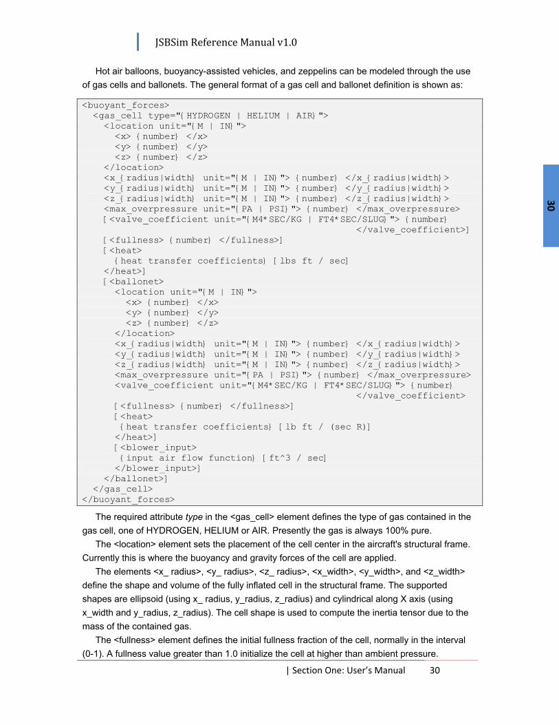
Hot air balloons, buoyancy-assisted vehicles, and zeppelins can be modeled through the use of gas cells and ballonets. The general format of a gas cell and ballonet definition is shown as:
<buoyant_forces> <gas_cell type="HYDROGEN | HELIUM | AIR"> <location unit="M | IN"> <x> number </x> <y> number </y> <z> number </z> </location> <x_radius|width unit="M | IN"> number </x_radius|width> <y_radius|width unit="M | IN"> number </y_radius|width> <z_radius|width unit="M | IN"> number </z_radius|width> <max_overpressure unit="PA | PSI"> number </max_overpressure> [<valve_coefficient unit="M4*SEC/KG | FT4*SEC/SLUG"> number </valve_coefficient>] [<fullness> number </fullness>] [<heat> heat transfer coefficients [lbs ft / sec] </heat>] [<ballonet> <location unit="M | IN"> <x> number </x> <y> number </y> <z> number </z> </location> <x_radius|width unit="M | IN"> number </x_radius|width> <y_radius|width unit="M | IN"> number </y_radius|width> <z_radius|width unit="M | IN"> number </z_radius|width> <max_overpressure unit="PA | PSI"> number </max_overpressure> <valve_coefficient unit="M4*SEC/KG | FT4*SEC/SLUG"> number </valve_coefficient> [<fullness> number </fullness>] [<heat> heat transfer coefficients [lb ft / (sec R)] </heat>] [<blower_input> input air flow function [ft^3 / sec] </blower_input>] </ballonet>] </gas_cell> </buoyant_forces>
The required attribute type in the <gas_cell> element defines the type of gas contained in the gas cell, one of HYDROGEN, HELIUM or AIR. Presently the gas is always 100% pure.
The <location> element sets the placement of the cell center in the aircraft's structural frame. Currently this is where the buoyancy and gravity forces of the cell are applied.
The elements <x_ radius>, <y_ radius>, <z_ radius>, <x_width>, <y_width>, and <z_width> define the shape and volume of the fully inflated cell in the structural frame. The supported shapes are ellipsoid (using x_ radius, y_radius, z_radius) and cylindrical along X axis (using x_width and y_radius, z_radius). The cell shape is used to compute the inertia tensor due to the mass of the contained gas.
The <fullness> element defines the initial fullness fraction of the cell, normally in the interval (0-1). A fullness value greater than 1.0 initialize the cell at higher than ambient pressure.

JSBSim Reference Manual v1.0
| Section One: User’s Manual 31
31
The element <max_overpressure> defines the maximum allowed cell overpressure with respect to the surrounding atmosphere. If the cell pressure is about to exceed this limit the excess gas is automatically and instantly valved off. This models a pressure relief valve of sufficient capacity mounted at the bottom of the cell.
The <valve_coefficient> element defines the capacity of the manual valve. The valve is considered to be located at the top of the cell. The valve coefficient determine the flow out of the cell according to:
where DeltaPressure is the difference between the internal pressure at the top of the cell and the surrounding atmosphere and ValveOpen is a non-negative number controlled by the user via the property buoyant_forces/gas-cell[x]/valve_open.
The element <heat> can contain zero or more FGFunction elements describing the heat flow from the atmosphere and surrounding environment into the gas cell. The unit is lb-ft/(sec-degR).
If there are no heat transfer functions at all the gas cell temperature will equal that of the surrounding atmosphere. A constant function returning 0 results in adiabatic behavior (i.e. no heat exchange at all with the environment).
The following is an example of how the heat flow due to conduction and radiation can be modelled:
<heat> <function name="buoyant_forces/gas-cell/dU_conduction"> <product> <value> 6282.25 </value> <!-- Surface area [ft2] --> <value> 0.05 </value> <!-- Conductivity [lb / (R ft sec)] --> <difference> <property> atmosphere/T-R </property> <property> buoyant_forces/gas-cell/temp-R </property> </difference> </product> </function> <function name="buoyant_forces/gas-cell/dU_radiation"> <product> <value> 0.1714e-8 </value> <!-- Stefan-Boltzmann's constant [Btu / (h ft^2 R^4)] --> <value> 0.05 </value> <!-- Emissivity [0,1] --> <value> 6282.25 </value> <!-- Surface area [ft2] --> <difference> <pow> <property> atmosphere/T-R </property> <value> 4.0 </value> </pow> <pow> <property> buoyant_forces/gas-cell/temp-R </property> <value> 4.0 </value> </pow> </difference> </product> </function> </heat>

JSBSim Reference Manual v1.0
| Section One: User’s Manual 32
32
A <gas_cell> element may contain zero or more <ballonet> elements. A ballonet is an air bag inside the gas cell in non-rigid or semi-rigid airships and is used to maintain the shape and volume of the gas cell/envelope and keep its internal pressure higher than that of the surrounding environment. It is common for such airships to have more than one ballonet, e.g. with one ballonet in the forward part and one in the aft part of the envelope the pitch attitude of the airship can be trimmed via the relative inflation of the two ballonets (as this moves part of the contained air forward or aft, respectively).
In JSBSim ballonets are modeled as being completely contained inside the enclosing gas cell (except for the inflow and outflow valves which serves air from and to the outside atmosphere).
3.1.5 Ground Reactions <contact type="BOGEY | STRUCTURE" name="string"> <location unit="IN | M"> <x> number </x> <y> number </y> <z> number </z> </location> <static_friction> number </static_friction> <dynamic_friction> number </dynamic_friction> <rolling_friction> number </rolling_friction> <spring_coeff unit="LBS/FT | N/M"> number </spring_coeff> <damping_coeff unit="LBS/FT/SEC | N/M/SEC"> number </damping_coeff> <damping_coeff_rebound unit="LBS/FT/SEC | N/M/SEC"> number </damping_coeff_rebound> <max_steer unit="DEG"> number | 0 | 360 </max_steer> <brake_group> NONE|LEFT|RIGHT|CENTER|NOSE|TAIL </brake_group> <retractable>0 | 1</retractable> <table type="CORNERING_COEFF"> </table> <relaxation_velocity> <rolling unit="FT/SEC | KTS | M/S"> number </rolling> <side unit="FT/SEC | KTS | M/S"> number </side> </relaxation_velocity> <force_lag_filter> <rolling> number </rolling> <side> number </side> </force_lag_filter> <wheel_slip_filter> number </wheel_slip_filter> </contact>
3.1.6 External Reactions JSBSim can model externally or arbitrarily applied forces and moments. Such a capability
might be needed to model a catapult, hook and wire capture device, tow rope, or parachute. Similar to the ground reactions specification, any external forces are defined in an external_reactions section:
<external_reactions> <!-- Interface properties, a.k.a. property declarations -->

JSBSim Reference Manual v1.0
| Section One: User’s Manual 33
33
[<property> ... <property>] <force name="name" frame="BODY|LOCAL|WIND" unit="unit"> [<function> ... </function>] <location unit="units"> <!-- location --> <x> value </x> <y> value </y> <z> value </z> </location> [<direction> <!-- optional for initial direction vector --> <x> value </x> <y> value </y> <z> value </z> </direction>] </force> </external_reactions>
Following initialization, the following properties are available:
external_reactions/force name/magnitude external_reactions/force name/x external_reactions/force name/y external_reactions/force name/z
The x, y, and z properties define a unit vector in the chosen frame. You can thus define a force magnitude and direct it an in any direction within the chosen frame (BODY, LOCAL, or STABILITY).
An example of a parachute modeled using the external reactions specification is as follows:
<external_reactions> <!-- "Declare" the reefing term --> <property>fcs/parachute_reef_pos_norm</property> <force name="parachute" frame="WIND"> <function> <product> <p> aero/qbar-psf </p> <p> fcs/parachute_reef_pos_norm </p> <v> 1.0 </v> <!-- Full drag coefficient --> <v> 20.0 </v> <!-- Full parachute area --> </product> </function> <!-- The location below is in structural frame (x positive aft), so this location describes a point 1 foot aft of the origin. In this case, the origin is the center. --> <location unit="FT"> <x>1</x> <y>0</y> <z>0</z> </location> <!-- The direction describes a unit vector. In this case, since the selected frame is the WIND frame, the "-1" x component describes a direction exactly opposite of the direction

JSBSim Reference Manual v1.0
| Section One: User’s Manual 34
34
into the wind vector. That is, the direction specified below is the direction that the drag force acts in. --> <direction> <x>-1</x> <y>0</y> <z>0</z> </direction> </force> </external_reactions>
3.1.7 Propulsion 3.1.8 Aerodynamics 3.1.9 Systems, Autopilot, and Flight Control 3.1.9.1 Mechanization of Components
Note that in many cases “properties” are referred to in the text and in the definition of the component. Properties are explained elsewhere, but suffice it to say for the moment that properties are like variables that are categorized into a tree structure, and accessible from the configuration file. Properties refer to various values within the simulation which serve an important purpose, such as roll rate, air density, drag force, etc.
3.1.9.1.1 Filter Component The filter component can simulate any first or second order filter, as well as an integrator. The
Tustin substitution is used to take filter definitions from Laplace space to the time domain. The general format for a filter specification is:
<typename name=”name”> <input> property </input> <c1> number|property </c1> [<c2> number|property </c2>] [<c3> number|property </c3>] [<c4> number|property </c4>] [<c5> number|property </c5>] [<c6> number|property </c6>] [<clipto> <min> number|property </min> <max> number|property </max> </clipto>] [<output> property </output>] </typename>
For a lag filter of the form,
the corresponding filter definition is:
<lag_filter name=”name”> <input> property </input> <c1> number|property </c1> [<clipto> <min> number|property </min> <max> number|property </max>

JSBSim Reference Manual v1.0
| Section One: User’s Manual 35
35
</clipto>] [<output> property </output>] </lag_filter>
As an example, for the specific filter:
600600
the corresponding filter definition could be:
<lag_filter name=”filter1”> <input> fcs/pitch-cmd </input> <c1> 600 </c1> </lag_filter>
For a lead-lag filter of the form:
The corresponding filter definition is:
<lead_lag_filter name=”name”> <input> property </input> <c1> number|property </c1> <c2> number|property </c2> <c3> number|property </c3> <c4> number|property </c4> [<clipto> <min> number|property </min> <max> number|property </max> </clipto>] [<output> property </output>] </lead_lag_filter>
For a washout filter of the form:
The corresponding filter definition is:
<washout_filter name=”name”> <input> property </input> <c1> number|property </c1> [<clipto> <min> number|property </min> <max> number|property </max> </clipto>] [<output> property </output>] </washout_filter>
For a second order filter of the form:
The corresponding filter definition is:

JSBSim Reference Manual v1.0
| Section One: User’s Manual 36
36
<second_order_filter name=”name”> <input> property </input> <c1> number|property </c1> <c2> number|property </c2> <c3> number|property </c3> <c4> number|property </c4> <c5> number|property </c5> <c6> number|property </c6> [<clipto> <min> number|property </min> <max> number|property </max> </clipto>] [<output> property </output>] </second_order_filter>
For an integrator of the form:
The corresponding definition is:
<integrator name=”name”> <input> property </input> <c1> number|property </c1> [<trigger> property </trigger>] [<clipto> <min> number|property </min> <max> number|property </max> </clipto>] [<output> property </output>] </integrator>
The trigger element shown in the integrator definition is a device used to prevent integrator wind-up. When the value of the property specified in the trigger element takes a non-zero value, the integrator ceases to integrate.
3.1.9.1.2 Switch Component The switch component models a switch – either an on/off or a multi-choice rotary switch. The
switch can represent a physical cockpit switch, or can represent a logical switch, where several conditions might need to be satisfied before a particular state is reached. The value of the switch – the output value – is chosen depending on the state of the switch. Each switch is comprised of two or more tests. Each test has a value associated with it. The first test that evaluates to true will set the output value of the switch according to the value parameter belonging to that test. Each test contains one or more conditions, which each must be logically related (if there are more than one) given the value of the logic parameter, and which takes the form:
property conditional property|value
e.g.
qbar GE 21.0
or,
roll_rate < pitch_rate

JSBSim Reference Manual v1.0
| Section One: User’s Manual 37
37
Within a test, additional tests can be specified, which allows for complex groupings of logical comparisons. The format of the switch component is as follows:
<switch name=”name”> <default value=”property|number/>” <test logic=”AND|OR” value=”property|number”> property conditional property|number … [<test logic=”AND|OR” value=”property|number”> property conditional property|number … </test>] </test> … [<clipto> <min> number|property </min> <max> number|property </max> </clipto>] [<output> property </output>] </switch>
Here’s an example:
<switch name=”Roll A/P Autoswitch”> <default value=”0.0”/> <test value=”fcs/roll-ap-error-summer”> ap/attitude_hold == 1 </test> </switch>
The above example specifies that the default value of the component (i.e. the output property of the component, addressed by the property, ap/roll-ap-autoswitch) is 0.0 if or when the attitude hold switch is selected (property ap/attitude_hold takes the value 1), the value of the switch component will be whatever value fcs/roll-ap-error-summer has. There is no input element for the switch component.
3.1.9.1.3 Sample and Hold Component The switch component supports a sample-and-hold function. To effect this, an example is
presented:
<switch name="fcs/roll-sample-and-hold-test"> <default value="attitude/psi-rad"/> <test value="fcs/roll-sample-and-hold-test"> ap/heading_hold == 1 </test> </switch>
Look carefully and you will see that the test takes on a value of itself if the condition is satisfied. In the example above, the default value is the heading (psi) in radians. Once the condition is satisfied (ap/heading_hold == 1), then the component holds the heading value at the time the condition was satisfied, and outputs that until such a time when the test condition is no longer satisfied. Restated, the default value (attitude/psi-rad) is output unless the condition is satisfied. If it is, then the test value (fcs/roll-sample-and-hold-test) is output. See the previous section for more information on the switch component.

JSBSim Reference Manual v1.0
| Section One: User’s Manual 38
38
3.1.9.1.4 Summer Component The Summer component sums two or more inputs. A bias can also be added in using the bias
keyword. The form of the summer component specification is:
<summer name=”name”> <input> [-]property </input> … <bias> number </bias> [<clipto> <min> number|property </min> <max> number|property </max> </clipto>] [<output> property </output>] </summer>
Note that in the case of an input property the property name may be immediately preceded by a minus sign.
Here’s an example of a summer component specification:
<summer name=”pid_sum”> <input> velocities/p-rad_sec </input> <input> -fcs/roll-ap-wing-leveler </input> <input> fcs/roll-ap-error-integrator </input> [<clipto> <min> -1.0 </min> <max> 1.0 </max> </clipto>] </summer>
Note that there can be only one bias statement per component.
3.1.9.1.5 Gain Component The gain component merely multiplies the input by a gain. The form of the gain component
specification is:
<pure_gain name="name"> <input> [-]property </input> [<gain> property|number </gain>] [<clipto> <min> number|property </min> <max> number|property </max> </clipto>] [<output> property </output>] </pure_gain>
The gain defaults to a value of 1.0 if not supplied. Note: as is the case with the Summer component, the input property name may be
immediately preceded by a minus sign to invert that signal.
3.1.9.1.6 Aerosurface Scaling Component This is a modified version of the simple gain component. The normal purpose for this
component is to take control inputs from a known domain and map them to a specified range. The form of the aerosurface scaling component specification is:
<aerosurface_scale name="name">

JSBSim Reference Manual v1.0
| Section One: User’s Manual 39
39
<input> [-]property </input> <zero_centered> true|false </zero_centered> [<domain> <min> number </min> <max> number </max> </domain>] <range> <min> number </min> <max> number </max> </range> [<gain> property|number </gain>] [<clipto> <min> number|property </min> <max> number|property </max> </clipto>] [<output> property </output>] </aerosurface_scale >
The gain is optional and defaults to 1.0. If the domain is not supplied, min and max default to –1.0 and +1.0, respectively. The “zero_centered” element specifies how the domain will be mapped to the range. If the zero_centered element is set to true (which is the default if it is not supplied) then the domain from the minimum (negative) value to zero is mapped to the range minimum (negative) to zero. The domain from zero to maximum is linearly mapped into the range from zero to the maximum range. Otherwise, the mapping is linear from the domain min-to-max span into the range min-to-max span. The center value may not correspond to zero.
For instance, the normal and expected ability of a pilot to push or pull on a control stick is about 50 pounds. The input to the pitch channel block diagram of a flight control system is in units of pounds. Yet, the joystick control input is usually in a range from –1 to +1. The following component definition takes joystick inputs from –1 to +1 and maps them to ±50.
<aerosurface_scale name="Pitch Command"> <input> fcs/pitch-cmd-norm </input> <range> <min> -50 </min> <max> 50 </max> </range> </aerosurface_scale >
Note: as is the case with the Summer component, the input property name may be immediately preceded by a minus sign to invert that signal.
3.1.9.1.7 Scheduled Gain Component The scheduled gain component multiplies the input by a variable gain that is dependent on
another property (such as qbar, altitude, etc.). The lookup mapping is in the form of a table. This kind of component might be used, for example, in a case where aerosurface deflection must only be commanded to acceptable settings – i.e at higher qbar the commanded elevator setting might be attenuated. The form of the scheduled gain component specification is:
<scheduled_gain name="name"> <input> [-]property </input> <table> <tableData>

JSBSim Reference Manual v1.0
| Section One: User’s Manual 40
40
… </tableData> </table> [<clipto> <min> [-]property|value </min> <max> [-]property|value </max> </clipto>] [<gain> property | value </gain>] [<output> property </output>] </scheduled_gain>
An overall <gain> may be supplied that is multiplicative with the scheduled gain. Note: as is the case with the Summer component, the input property name may be
immediately preceded by a minus sign to invert that signal. Here is an example of a scheduled gain component specification:
<scheduled_gain name="Pitch Scheduled Gain 1"> <input>fcs/pitch-gain-1</input> <gain>0.017</gain> <table> <independentVar>fcs/elevator-pos-rad</independentVar> <tableData> -0.68 -26.548 -0.595 -20.513 -0.51 -15.328 … 0.527 -20.513 0.612 -26.548 0.697 -33.433 </tableData> </table> </scheduled_gain>
In the example above, there is a table – a function of elevator angle in radians – which outputs a command in degrees. The overall GAIN value effects a degrees-to-radians conversion on the output of the table.
3.1.9.1.8 Deadband Component This is a component that allows for some “play” in a control path, in the form of a dead zone,
or deadband. The form of the deadband component specification is:
<deadband name="Windup Trigger"> <input> [-]property </input> <width> number </width> [<clipto> <min> [-]property|value </min> <max> [-]property|value </max> </clipto>] [<output> property </output>] </deadband>
The width value is the total deadband region within which an input will produce no output. For example, say that the width value is 2.0. If the input is between –1.0 and +1.0, the output will be zero.

JSBSim Reference Manual v1.0
| Section One: User’s Manual 41
41
3.1.9.1.9 Hysteresis Component [not yet modeled]
3.1.9.1.10 Limiter Component There is currently not a unique limiter component. However, the functionality of a limiter can
be achieved by using a gain component with the clipto argument set with the minimum and maximum limits.
3.1.9.1.11 Positive or Negative Value Component There exists no unique positive or negative value component. However, the functionality of
such a component can be achieved by using a gain component with the clipto argument set to 0.0 and a maximum limit (for a positive value component), or having the clipto argument set to the minimum limit and 0.0 (for a negative value component). In this way, only half of the input domain will be accepted (either the positive domain or the negative domain).
3.1.9.1.12 Absolute Value Component The functionality of an absolute value component could be implemented by a modified gain
component, though such a modification has not yet been made. An absolute value could also be achieved through the use of an FCS Function component.
3.1.9.1.13 Kinematic Component This component models the action of a moving effector, such as an aerosurface or other
mechanized entity such as a landing gear strut for the purpose of effecting vehicle control or configuration. The form of the component specification is:
<kinematic name="Gear Control"> <input> [-]property </input> <traverse> <setting> <position> number </position> <time> number </time> </setting> … </traverse> [<clipto> <min> [-]property|value </min> <max> [-]property|value </max> </clipto>] [<gain> property | value </gain>] [<output> property </output>] </kinematic>
The position is the position that the component takes, and the lag is the time it takes to get to that position from an adjacent setting. For example:
<kinematic name="Gear Control"> <input>gear/gear-cmd-norm</input> <traverse> <setting> <position>0</position> <time>0</time> </setting> <setting>

JSBSim Reference Manual v1.0
| Section One: User’s Manual 42
42
<position>1</position> <time>5</time> </setting> </traverse> <output>gear/gear-pos-norm</output> </kinematic>
In this case, it takes 5 seconds to get to a 1 setting. As this is a software mechanization of a servo-actuator, there will often be an OUTPUT specified, such as to an elevator, gear actuator, aileron, or other mechanism.
3.1.9.1.14 FCS Function Component One of the most recent additions to the FCS component set is the FCS Function component.
This component allows a function to be created when no other component is suitable. The function component is defined as follows:
<fcs_function name="Windup Trigger"> [<input> [-]property </input>] <function> … </function> [<clipto> <min> [-]property|value </min> <max> [-]property|value </max> </clipto>] [<output> property </output>] </ fcs_function >
The function definition itself can include a nested series of products, sums, quotients, etc. as well as trig and other math functions. Here’s an example of a function (from an aero specification):
<function name="aero/coefficient/CDo"> <description>Drag_at_zero_lift</description> <product> <property>aero/qbar-psf</property> <property>metrics/Sw-sqft</property> <table> <independentVar>velocities/mach</independentVar> <tableData> 0.0000 0.0220 0.2000 0.0200 0.6500 0.0220 0.9000 0.0240 0.9700 0.0500 </tableData> </table> </product> </function>
3.1.9.1.15 Actuator Component The actuator can be modeled as a "perfect actuator", with the Output being set directly to the
input. The actuator can be made more "real" by specifying any/all of the following additional effects that can be applied to the actuator. In order of application to the input signal, these are:

JSBSim Reference Manual v1.0
| Section One: User’s Manual 43
43
System lag (input lag, really) Rate limiting Deadband Hysteresis (mechanical hysteresis) Bias (mechanical bias) Position limiting ("hard stops") There are also several malfunctions that can be applied to the actuator by setting a property
to true or false (or 1 or 0). Syntax:
<actuator name=”name”> <input> [-]property </input> <lag> number </lag> <rate_limit> number <rate_limit> <bias> number </bias> <deadband_width> number </deadband_width> <hysteresis_width> number </hysteresis_width> [<clipto> <min> [-]property|value </min> <max> [-]property|value </max> </clipto>] [<output> property </output>] </actuator>
Example:
<actuator name=”fcs/gimbal_pitch_position”> <input> fcs/gimbal_pitch_command </input> <lag> 60 </lag> <rate_limit> 0.085 <rate_limit> <!-- 5 degrees/sec --> <bias> 0.002 </bias> <deadband_width> 0.002 </deadband_width> <hysteresis_width> 0.05 </hysteresis_width> <clipto> <!-- +/- 10 degrees --> <min> -0.17 </min> <max> 0.17 </max> </clipto> </actuator>
3.1.9.1.16 Sensor Component When the flight control system uses “sensed” values such as qbar or orientation, the sensed
values are taken from the environment model, and are modeled as “perfect sensors”. That is, the values were taken directly from the equations of motion, without attempting to make them look as though they had come from a sensing device (gyro, pitot tube, etc.) – with the associated imperfections that those devices can introduce. Imperfections can include noise, drift, and truncation of precision, etc. A bias can be introduced; a bias is simply an offset introduced to the sensor.
The sensor component models imperfections and increases the realism of the control system. The only required element in the sensor definition is the input element. In that case, no degradation would be modeled, and the output would simply be the input.
For adding noise, if the type is PERCENT, then the value supplied is understood to be a
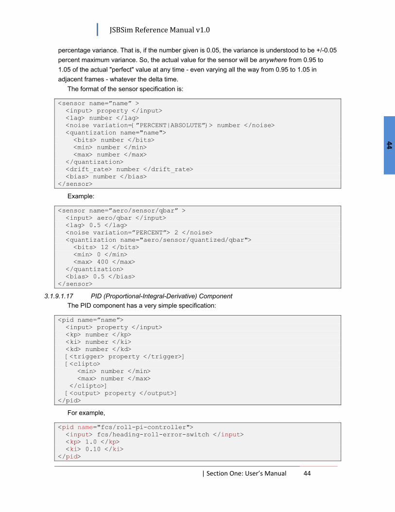
JSBSim Reference Manual v1.0
| Section One: User’s Manual 44
44
percentage variance. That is, if the number given is 0.05, the variance is understood to be +/-0.05 percent maximum variance. So, the actual value for the sensor will be anywhere from 0.95 to 1.05 of the actual "perfect" value at any time - even varying all the way from 0.95 to 1.05 in adjacent frames - whatever the delta time.
The format of the sensor specification is:
<sensor name=”name” > <input> property </input> <lag> number </lag> <noise variation=”PERCENT|ABSOLUTE”> number </noise> <quantization name="name"> <bits> number </bits> <min> number </min> <max> number </max> </quantization> <drift_rate> number </drift_rate> <bias> number </bias> </sensor>
Example:
<sensor name=”aero/sensor/qbar” > <input> aero/qbar </input> <lag> 0.5 </lag> <noise variation=”PERCENT”> 2 </noise> <quantization name="aero/sensor/quantized/qbar"> <bits> 12 </bits> <min> 0 </min> <max> 400 </max> </quantization> <bias> 0.5 </bias> </sensor>
3.1.9.1.17 PID (Proportional-Integral-Derivative) Component The PID component has a very simple specification:
<pid name=”name”> <input> property </input> <kp> number </kp> <ki> number </ki> <kd> number </kd> [<trigger> property </trigger>] [<clipto> <min> number </min> <max> number </max> </clipto>] [<output> property </output>] </pid>
For example,
<pid name="fcs/roll-pi-controller"> <input> fcs/heading-roll-error-switch </input> <kp> 1.0 </kp> <ki> 0.10 </ki> </pid>
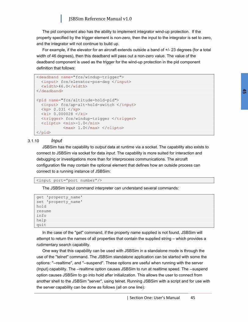
JSBSim Reference Manual v1.0
| Section One: User’s Manual 45
45
The pid component also has the ability to implement integrator wind-up protection. If the property specified by the trigger element is non-zero, then the input to the integrator is set to zero, and the integrator will not continue to build up.
For example, if the elevator for an aircraft extends outside a band of +/- 23 degrees (for a total width of 46 degrees), then this deadband will pass out a non-zero value. The value of the deadband component is used as the trigger for the wind-up protection in the pid component definition that follows:
<deadband name="fcs/windup-trigger"> <input> fcs/elevator-pos-deg </input> <width>46.0</width> </deadband> <pid name="fcs/altitude-hold-pid"> <input> fcs/ap-alt-hold-switch </input> <kp> 0.031 </kp> <ki> 0.000028 </ki> <trigger> fcs/windup-trigger </trigger> <clipto> <min>-1.0</min> <max> 1.0</max> </clipto> </pid>
3.1.10 Input JSBSim has the capability to output data at runtime via a socket. The capability also exists to
connect to JSBSim via socket for data input. The capability is more suited for interaction and debugging or investigations more than for interprocess communications. The aircraft configuration file may contain the optional element that defines how an outside process can connect to a running instance of JSBSim:
<input port=”port number”/>
The JSBSim input command interpreter can understand several commands:
get 'property_name' set 'property_name' hold resume info help quit
In the case of the ''get'' command, if the property name supplied is not found, JSBSim will attempt to return the names of all properties that contain the supplied string – which provides a rudimentary search capability.
One way that this capability can be used with JSBSim in a standalone mode is through the use of the ''telnet'' command. The JSBSim standalone application can be started with some the options: ''--realtime'', and ''--suspend''. These options are useful when running with the server (Input) capability. The --realtime option causes JSBSim to run at realtime speed. The --suspend option causes JSBSim to go into hold after initialization. This allows the user to connect from another shell to the JSBSim "server", using telnet. Running JSBSim with a script and for use with the server capability can be done as follows (all on one line):

JSBSim Reference Manual v1.0
| Section One: User’s Manual 46
46
src/jsbsim --script=scripts/c1723.xml --realtime --suspend
With the above command line, JSBSim will initialize and hold. A connection via telnet to JSBSim from a different shell can then be made:
telnet host port
For example:
telnet localhost 1137
JSBSim responds over the socket:
$ telnet localhost 1137 Trying 127.0.0.1... Connected to zeus. Escape character is '^]'. Connected to JSBSim server JSBSim>
Typing ''info'' gives important information about the simulation run:
JSBSim> info JSBSim version: 0.9.13 Config File version: 2.0 Aircraft simulated: Cessna C-172 Simulation time: 0.008
Property values can be set or retrieved using the get and set commands. If the exact property name is unknown, the get command can also be used to search for all properties that contain the given string (this capability can only be used while in hold):
JSBSim> get /inertia inertia/mass-slugs inertia/weight-lbs inertia/cg-x-ft inertia/cg-y-ft inertia/cg-z-ft
The value for a specific property can be retrieved using the get command:
JSBSim> get inertia/cg-x-ft inertia/cg-x-ft = 43.886700
Setting a property value is done as follows (for example):
JSBSim> set ap/elevator_cmd 1
Note that the “=” symbol is not used.
3.1.11 Output An <output> specification in a vehicle configuration file is optional, but in order to get any data
logged during a run, the simulation must be told what to output, where to send the data, and at what rate to output data.
The <output> section can optionally be included in the vehicle configuration file, or it can be specified in a standalone file, the name of which can be supplied on the command line for the
JSBSim Reference Manual v1.0
| Section One: User’s Manual 47
47
standalone executable. This approach can be useful when different sets of variables are to be logged on different occasions. The format of the <output> section is the same regardless of which approach is taken.
3.2 Engines 3.2.1 Piston 3.2.2 Turbine 3.2.3 Turboprop 3.2.4 Rocket 3.2.5 Electric 3.3 Thrusters 3.3.1 Propeller 3.3.2 Nozzle 3.3.3 Direct 3.4 Initialization 3.5 Scripts

JSBSim Reference Manual v1.0
| Section One: User’s Manual 48
48
4. Input/output
4.1 Socket I/O 4.2 File and Console I/O
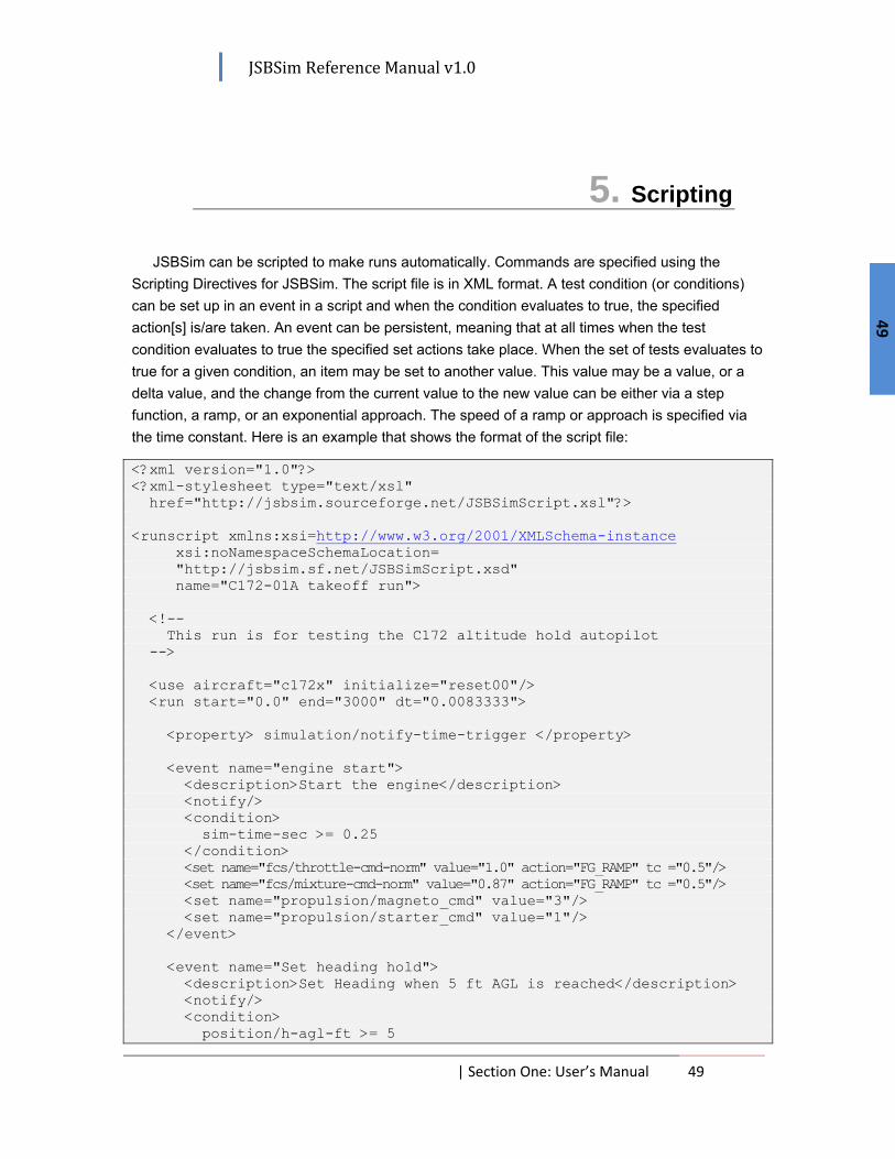
JSBSim Reference Manual v1.0
| Section One: User’s Manual 49
49
5. Scripting
JSBSim can be scripted to make runs automatically. Commands are specified using the Scripting Directives for JSBSim. The script file is in XML format. A test condition (or conditions) can be set up in an event in a script and when the condition evaluates to true, the specified action[s] is/are taken. An event can be persistent, meaning that at all times when the test condition evaluates to true the specified set actions take place. When the set of tests evaluates to true for a given condition, an item may be set to another value. This value may be a value, or a delta value, and the change from the current value to the new value can be either via a step function, a ramp, or an exponential approach. The speed of a ramp or approach is specified via the time constant. Here is an example that shows the format of the script file:
<?xml version="1.0"?> <?xml-stylesheet type="text/xsl" href="http://jsbsim.sourceforge.net/JSBSimScript.xsl"?> <runscript xmlns:xsi=http://www.w3.org/2001/XMLSchema-instance xsi:noNamespaceSchemaLocation= "http://jsbsim.sf.net/JSBSimScript.xsd" name="C172-01A takeoff run"> <!-- This run is for testing the C172 altitude hold autopilot --> <use aircraft="c172x" initialize="reset00"/> <run start="0.0" end="3000" dt="0.0083333"> <property> simulation/notify-time-trigger </property> <event name="engine start"> <description>Start the engine</description> <notify/> <condition> sim-time-sec >= 0.25 </condition> <set name="fcs/throttle-cmd-norm" value="1.0" action="FG_RAMP" tc ="0.5"/> <set name="fcs/mixture-cmd-norm" value="0.87" action="FG_RAMP" tc ="0.5"/> <set name="propulsion/magneto_cmd" value="3"/> <set name="propulsion/starter_cmd" value="1"/> </event> <event name="Set heading hold"> <description>Set Heading when 5 ft AGL is reached</description> <notify/> <condition> position/h-agl-ft >= 5
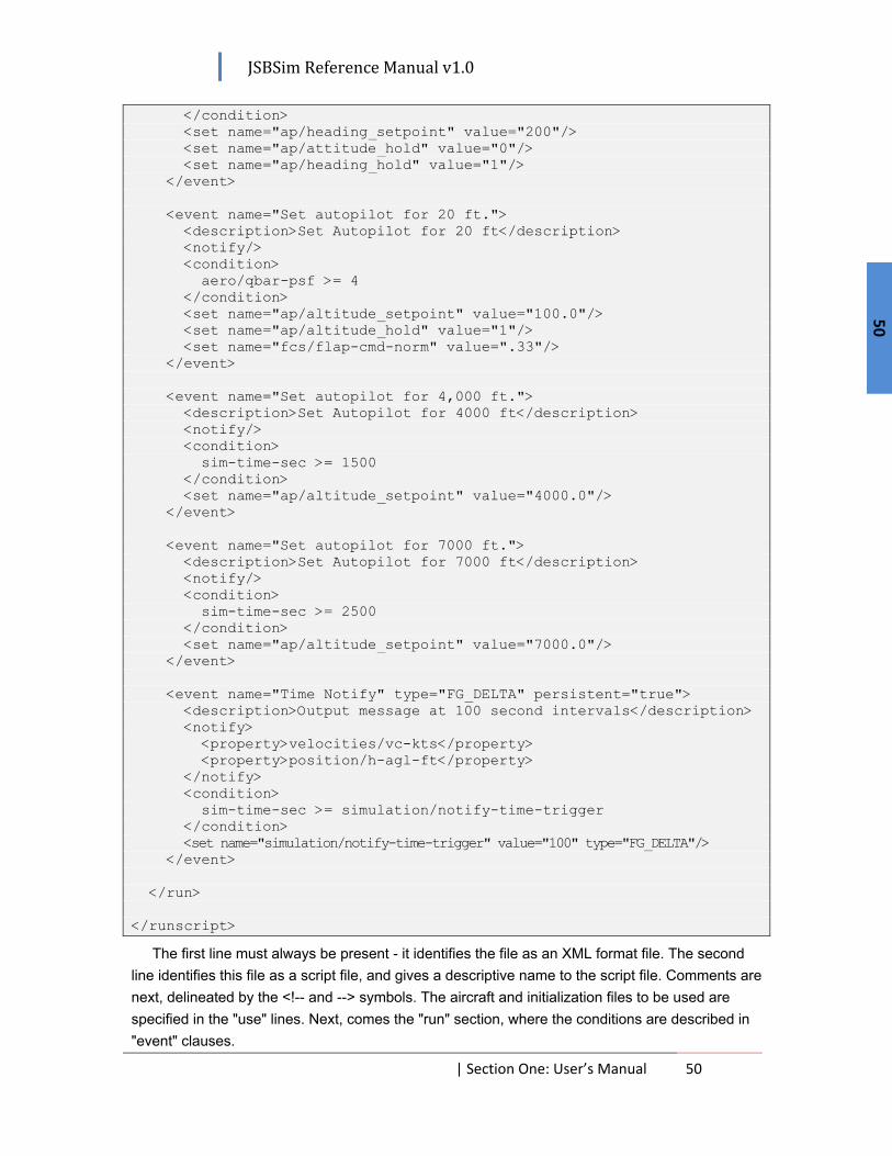
JSBSim Reference Manual v1.0
| Section One: User’s Manual 50
50
</condition> <set name="ap/heading_setpoint" value="200"/> <set name="ap/attitude_hold" value="0"/> <set name="ap/heading_hold" value="1"/> </event> <event name="Set autopilot for 20 ft."> <description>Set Autopilot for 20 ft</description> <notify/> <condition> aero/qbar-psf >= 4 </condition> <set name="ap/altitude_setpoint" value="100.0"/> <set name="ap/altitude_hold" value="1"/> <set name="fcs/flap-cmd-norm" value=".33"/> </event> <event name="Set autopilot for 4,000 ft."> <description>Set Autopilot for 4000 ft</description> <notify/> <condition> sim-time-sec >= 1500 </condition> <set name="ap/altitude_setpoint" value="4000.0"/> </event> <event name="Set autopilot for 7000 ft."> <description>Set Autopilot for 7000 ft</description> <notify/> <condition> sim-time-sec >= 2500 </condition> <set name="ap/altitude_setpoint" value="7000.0"/> </event> <event name="Time Notify" type="FG_DELTA" persistent="true"> <description>Output message at 100 second intervals</description> <notify> <property>velocities/vc-kts</property> <property>position/h-agl-ft</property> </notify> <condition> sim-time-sec >= simulation/notify-time-trigger </condition> <set name="simulation/notify-time-trigger" value="100" type="FG_DELTA"/> </event> </run> </runscript>
The first line must always be present - it identifies the file as an XML format file. The second line identifies this file as a script file, and gives a descriptive name to the script file. Comments are next, delineated by the <!-- and --> symbols. The aircraft and initialization files to be used are specified in the "use" lines. Next, comes the "run" section, where the conditions are described in "event" clauses.
JSBSim Reference Manual v1.0
| Section One: User’s Manual 51
51
A delay can be specified for an event, so that it executes a certain number of seconds after it is triggered. An event can be a notify-only event. That is, you do not have to specify actions for an event, it can exist to notify the user of some kind of event. The conditional tests are modeled using a “standard” JSBSim conditional construct that is also used in the flight control switch component. When coupled with the property declaration capability and the notify flag, some interesting effects can be achieved. One of those is a repeating notification that is printed at time or altitude intervals. See the Time Notify event in the above example.
Formal documentation for the JSBSim Script Language can be found at, http://jsbsim.sourceforge.net/JSBSim/JSBSimScript.xsd.html
JSBSim Reference Manual v1.0
| Section Two: Programmer's Manual 52
52
Section 2: Programmer's Manual

JSBSim Reference Manual v1.0
| Section Two: Programmer's Manual 53
53
1. Overview
One of the specific intentions of JSBSim is to make sure it is relatively easy to incorporate into a small or large simulation program. As often happens with simulation programs (and software applications in general) "feature creep" sets in and the program code blossoms into a larger-than-intended product. In the case of JSBSim, we have attempted to maintain the code base as small as possible, but at first glance it can still be overwhelming.
Let’s think for a moment about what should be present in a simulator. Of course, the aerodynamic characteristics of the vehicle need to be modeled – and that in turn depends on the atmosphere. Winds can be modeled, too. Gravity needs to be modeled. Clearly, the environment needs to be modeled. As for the aircraft itself, apart from the aerodynamic characteristics which cause forces and moments to be applied, propulsive effects must be modeled, buoyancy, ground reactions, ground contact, and other externally applied forces can be modeled. Flight control characteristics must be modeled, and other systems can be modeled as well (such as an autopilot, other Guidance, Navigation, and Control (GNC) systems, or even electric or hydraulic systems). Finally, the forces and moments cause the aircraft or vehicle to move, and so the location and orientation of the vehicle must be tracked and propagated over time. There are of course a lot of models to keep track of, so some kind of model management or executive is needed. It’s important to be able to input data to and extract data from the simulation, so an input and output capability is needed. Lastly, there are convenience or utility functions such as functions, tables, and quaternions, which facilitate the functioning of the models.
For JSBSim, the C++ programming language was chosen to implement the above mentioned models and ideas in program code. Over the years, I have fielded questions from people who ask why I chose that language instead of something else. Some old-timers have sworn by Fortran as being the language of choice for engineering applications. More recently, some have suggested to me that Java would be good for implementing a flight dynamics model. You could use any language, I suppose, but given the current state of the standard C++ language across many platforms, the ready availability of excellent compilers and IDEs (Integrated Development Environments) – even free ones – and the similarity of C++ to the C programming language, the choice of C++ seems natural. It is one of the more widely known and used languages today. Object oriented programming is well supported by C++. I’ve also found that programming in C++ is fun.
The C++ programming language is ideal for use in flight simulation software in part because of its support of the primary object-oriented concepts: polymorphism, inheritance, encapsulation, and abstraction.
Polymorphism (i.e. “having many forms”) is a characteristic of objects that operate differently internally, but have the same interface. For example, the JSBSim implementation of a flight control system (FCS) consists of various classes of filters, switches, and gains that each have a unique internal implementation. The public interface to the components consists of the Run() and

JSBSim Reference Manual v1.0
| Section Two: Programmer's Manual 54
54
GetOutput() methods, which are both virtual member functions of the component base class. These two methods are overridden in derived classes that represent specific components with unique behavior. Each instance of a component is referred to by the base class pointer, but the behavior is determined by the logic defined within the Run() method of the specific derived component class.
Inheritance is the derivation of a class from another in order to provide base class characteristics to the derived class. Using the example of the JSBSim FCS component classes again, each of the specific component classes (switch, summer, filter, etc.) is derived from a more generic component class that features characteristics that all components share. Inheritance is a common way to implement polymorphism.
Encapsulation is the concept of hiding and protecting data in a class, preventing corruption by outside processes. For example, the output of the FCS components may only be retrieved, and not modified. In addition, some of the JSBSim FCS components store past values. These should never be accessible by any other part of the program. Abstraction is “the elimination of the irrelevant and the amplification of the essential”. The FCS component base class, for instance, provides the two simple functions Run() and GetOutput() that are used to operate a component. The details of how each specific component operates do not need to be exposed.
The Standard Template Library (STL) is a library of containers and algorithms. The STL provides containers such as the vector class that operate like arrays that shrink or grow as needed. This capability is particularly useful in JSBSim, because the number of engines, coefficients, FCS components, etc. is unknown until the program is executed.
In the simplest use, where JSBSim is to be called upon from a tiny application that simply runs a command script for an aircraft, here is an example of how JSBSim could be used:
#include <FGFDMExec.h> int main(int argc, char **argv) JSBSim::FGFDMExec FDMExec; FDMExec.LoadScript(argv[1]); while (FDMExec.Run());
The above code can actually be compiled and run. If the above code replaces the JSBSim.cpp file in the basic JSBSim distribution, typing "make" should make the code. It could subsequently be run by simply typing:
src/jsbsim scripts/my_script_name.xml
The "Executive" class object, "FGFDMExec" does most of the work in setting up and running JSBSim. In words, the above program – when compiled and run – will create an instance of an FGFDMExec object, load a script (which in turn loads an aircraft file and an initial conditions file), and cyclically run the simulation until the simulation completes as specified in the script.
For creating an application that runs inside a larger simulation program, where command inputs are made via joystick and outputs drive a visual scene, the following code excerpt shows how this can be done:

JSBSim Reference Manual v1.0
| Section Two: Programmer's Manual 55
55
int initialize_flight_dynamics(char *name) FDMExec = new FGFDMExec(); FDMExec->LoadAircraft(name); FDMExec->DoTrim(mode); int run_flight_dynamics() copy_inputs_to_jsbsim(); FDMExec->Run(); copy_outputs_from_jsbsim();
The above two functions would be linked into the main program code, with the initialization function being called (as the name suggests) at initialization, and the latter function being called cyclically during runtime. The "copy_inputs_to_jsbsim" and "copy_outputs_from_jsbsim" functions are separate functions that would need to be written. Those two functions would take care of providing inputs to and extracting outputs from JSBSim. That process will be discussed later.
In the following sections, the layers and processes will be looked at from a high level, followed by a more detailed look.

JSBSim Reference Manual v1.0
| Section Two: Programmer's Manual 56
56
2. Class Heirarchy
There are roughly 70 C++ classes that comprise JSBSim. The code files themselves are distributed into subdirectories based on function. There are math classes, classes that aid input/output and initialization, model classes, and basic classes. There are some key inheritance relationships that should be understood. For instance, there is a model class (FGModel), from which specific model classes inherit, and base FGEngine, FGFCSComponent, FGThruster, and FGParameter classes. These inheritance relationships are shown in Figure 1.
The collection of classes that make up the JSBSim framework resembles a “family tree” with a common parent at the head of the hierarchy. This graphically illustrates the concept of inheritance and – indirectly – code reuse. An entire class framework does not necessarily have to conform to a completely hierarchical arrangement. In JSBSim, several classes represent generic objects or concepts that are each fully realized in derived classes. These base classes can be viewed as providing the abstract interface that is used to access each of the derived objects. There are also operations and attributes (a fancy name for class member variables) that are common to almost all classes, so it makes sense to implement those characteristics in a common base class. For instance, the framework base class (FGJSBBase) implements a messaging capability, Figure 1 JSBSim class heirarchy
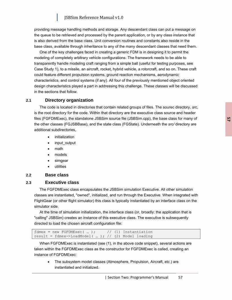
JSBSim Reference Manual v1.0
| Section Two: Programmer's Manual 57
57
providing message handling methods and storage. Any descendant class can put a message on the queue to be retrieved and processed by the parent application, or by any class instance that is also derived from the base class. Unit conversion routines and constants also reside in the base class, available through inheritance to any of the many descendant classes that need them.
One of the key challenges faced in creating a generic FDM is in designing it to permit the modeling of completely arbitrary vehicle configurations. The framework needs to be able to transparently handle modeling craft ranging from a simple ball (useful for testing purposes, see Case Study 1), to a missile, an aircraft, rocket, hybrid vehicle, a rotorcraft, and so on. These craft could feature different propulsion systems, ground reaction mechanisms, aerodynamic characteristics, and control systems (if any). All four of the previously mentioned object oriented design characteristics played a part in addressing this challenge. These classes will be discussed in the sections that follow.
2.1 Directory organization The code is located in directories that contain related groups of files. The sourec directory, src,
is the root directory for the code. Within that directory are the executive class source and header files (FGFDMExec), the standalone JSBSim source file (JSBSim.cpp), the base class for many of the other classes (FGJSBBase), and the state class (FGState). Underneath the src/ directory are additional subdirectories,
• initialization • input_output • math • models • simgear • utilities
2.2 Base class 2.3 Executive class
The FGFDMExec class encapsulates the JSBSim simulation Executive. All other simulation classes are instantiated, "owned", initialized, and run through the Executive. When integrated with FlightGear (or other flight simulator) this class is typically instantiated by an interface class on the simulator side.
At the time of simulation initialization, the interface class (or, broadly: the application that is "calling" JSBSim) creates an instance of this executive class. The executive is subsequently directed to load the chosen aircraft configuration file:
fdmex = new FGFDMExec( … ); // (1) Instantiation result = fdmex->LoadModel( … ); // (2) Model loading
When FGFDMExec is instantiated (see (1), in the above code snippet), several actions are taken within the FGFDMExec class as the constructor for FGFDMExec is called, creating an instance of FGFDMExec:
• The subsystem model classes (Atmosphere, Propulsion, Aircraft, etc.) are instantiated and initialized.

JSBSim Reference Manual v1.0
| Section Two: Programmer's Manual 58
58
• The subsystem models are scheduled - that is a list of models is made that will be called in order when each frame is cyclically processed.
After the Executive is created, the aircraft model is loaded. When an aircraft model is loaded, the config file (the name of which is supplied in the LoadModel() function of the Executive class) is parsed and for each of the sections of the config file (propulsion, flight control, etc.) the corresponding Load() method is called (e.g. FGFCS::Load() is called to load the flight control system parameters).
Subsequent to the creation of the executive and loading of the model, initialization is performed. Initialization involves copying control inputs from the controlling application (FlightGear, or the main() application in the case of JSBSim standalone) into the appropriate JSBSim data storage locations, configuring it for the set of user-supplied initial conditions, and then copying state variables from JSBSim, back into the controlling application. The state variables are used to drive the instrument displays and to place the vehicle model in world space for visual rendering:
copy_to_JSBsim(); // copy control inputs to JSBSim fdmex->RunIC(); // loop JSBSim once w/o integrating copy_from_JSBsim(); // update the bus
Once initialization is complete, cyclic execution proceeds:
copy_to_JSBsim(); // copy control inputs to JSBSim fdmex->Run(); // execute JSBSim copy_from_JSBsim(); // update the bus
Figure 2 The JSBSim FGFDMExec class and initialization process.

JSBSim Reference Manual v1.0
| Section Two: Programmer's Manual 59
59
JSBSim can be used in a standalone mode by creating a compact stub program that effectively performs the same progression of steps as outlined above for the integrated version, but with two exceptions. First, the copy_to_JSBSim() and copy_from_JSBSim() functions are not used because the control inputs are handled directly by the scripting facilities and outputs are handled by the output (data logging) class. Second, the name of a script file can be supplied to the stub program. Scripting (see FGScript) provides a way to supply command inputs to the simulation:
FDMExec = new JSBSim::FGFDMExec(); FDMExec->LoadScript( ScriptName ); // the script loads the aircraft and ICs result = FDMExec->Run(); while (result) // cyclic execution result = FDMExec->Run(); // execute JSBSim
The standalone mode has been useful for verifying changes before committing updates to the source code repository. It is also useful for running sets of tests that reveal some aspects of simulated aircraft performance, such as range, time-to-climb, takeoff distance, etc.
2.4 Manager classes 2.5 Model classes
When it comes down to it, the job of a 6DoF flight dynamics model (FDM) is to answer these questions at the end of each cyclic frame:
• Where am I (latitude, longitude, altitude)? • Which way am I oriented (pitch, yaw, roll)?
In accomplishing this, the FDM needs to know the forces and moments that are acting on the aircraft at any moment. As a prerequisite to this, the FDM must know the environmental characteristics, control inputs, etc.
JSBSim is comprised of classes that include specific model classes. Model classes are those classes that descend from the FGModel class, are executed in order during each cyclic frame, and which represent real physical objects, or which manage collections of real, physical objects. The FGPropulsion class, for instance, manages a collection of engines (FGEngine objects), the FGFCS class manages a collection of flight control components (FGFCSComponent objects), the FGGroundReactions class manages a collection of landing gear (FGLGear objects),and the FGAerodynamics class manages a list of aerodynamic forces and moments (FGFunction objects). The list of model classes is as follows (presented in order of execution):
• Input • Atmosphere • FCS (a collection manager class) • Propulsion (a collection manager class) • MassBalance • Aerodynamics (a collection manager class) • Inertial • GroundReactions (a collection manager class)

JSBSim Reference Manual v1.0
| Section Two: Programmer's Manual 60
60
• Aircraft • Propagate • Auxiliary • Output
The Executive class (FGFDMExec) both stores its own private-access pointers to the instances of these classes, and manages sequential and cyclical execution of each class instance over each frame.
A description of the above mentioned Model class objects is presented in the following sections.
2.5.1 Input The FGInput class implements the input capability for JSBSim, and is the first FGModel-
derived object scheduled for execution in the frame. After the model classes are instantiated and initialized, the aircraft files are loaded. As part of
that process, the Load() method for FGInput is called - '''if''' there is an <input> element in the aircraft configuration file being loaded.
The FGInput::Load() method creates an instance of an FGfdmSocket class, passing the port number as an argument. This socket sets up the communication interface and begins listening so it is ready to accept a connection request from another process.
At runtime, the FGInput::Run() method is called. If data has been received through the socket, the data is processed, parsed and examined for the presence of known keywords. If those keywords are found, the appropriate action is taken.
2.5.2 Atmosphere The Atmosphere model (FGAtmosphere class) models the 1976 standard atmosphere. It also
models winds and turbulence, but that portion is experimental at this time. The atmosphere class can either calculate the basic properties (pressure, density,
temperature) or those parameters can be set from an external process. The atmospheric properties are calculated in the Run() method, executed each frame. If the atmospheric properties are supplied by an external source, the CalculateDerived() function is called. If the standard properties are calculated by the FGAtmosphere class itself (the normal approach), then the current altitude is first retrieved, and then the Calculate() function is called to determine the current pressure, density, and temperature. Subsequent to that, the CalculateDerived() function is called to compute additional values that depend on the standard atmospheric values. Among the additional parameters that are calculated within the CalculateDerived() function are speed of sound and density altitude.
The FGAtmosphere class also serves as a base class for other atmosphere models. There is a subdirectory, atmosphere/, under which can be found two additional atmosphere models, FGMSIS and FGMars. These are experimental, but FGMSIS has been tested and works well.
2.5.3 FCS (Flight Control System) The FCS class (FGFCS) encapsulates the Flight Control System (FCS) functionality. This
class owns and contains (manages) the list of FGFCSComponent-derived objects that define the control system for the loaded aircraft. FGFCS also provides function calls to read and set various

JSBSim Reference Manual v1.0
| Section Two: Programmer's Manual 61
61
standard flight control parameters. The constructor for FGFCS initializes various parameters and also calls bind(), which binds
property names (text strings) with access methods (methods that get and set values, such as GetThrottleCmd() and SetThrottlePos() for getting and setting throttle values). The Property System is what allows property names to be specified in configuration files and accessed at run time.
When FGFCS::Load() is called, the section of the aircraft configuration file demarked by the <flight_control> element tags is parsed. The flight control definition can have any number of channels, each of which contains a sequence of FCS component definitions. When each of the component definitions is parsed, it creates an instance of the associated class object, and a pointer to that object is pushed onto a storage "array" - actually, a Standard Template Library vector container.
Three separate vector containers are used, because there are two flight control objects can be specified for any aircraft model: an autopilot, and a flight control system. The third vector may contain pointers to sensor objects. This allows sensor values to be calculated first, and then an entire set of flight control components (representing a set of control laws) may be executed before a second set of components is run.
At runtime, the list of components is executed in sequential order, with each component Run() method being called.
2.5.4 Propulsion The propulsion class (FGPropulsion) manages a collection of zero or more engine objects of
any type or combination of types. At initialization, the propulsion section of the configuration file is read and, if any engines are encountered, an instance of that engine is created and added to the engine array. At runtime, the propulsion class runs each engine in the list in sequence. Each engine calculates the engine parameters, fuel usage, etc. and finally returns the forces and moments that the engine exerts on the airframe. Fuel/propellants are subtracted from the tanks (FGTank).
Several different engine types are modeled in JSBSim:
• Piston engine (which supports turbocharging), FGPiston class • Turbine engine, FGTurbine class • Turboprop engine, FGTurboProp class • Rocket engine, FGRocket class • Electric engine, FGElectric class
The engine-specific parameters are defined in the engine configuration file in XML format. Each engine "owns" a thruster object that is used to turn the engine power into a force. The thruster may be a propeller, a nozzle, or a direct pass-through object.
2.5.5 Mass & Balance Weight and balance modeling for JSBSim includes the calculation of moments of inertia,
center of gravity, and mass quantities. The FGMassBalance class handles mass properties calculations.
At initialization, the mass_balance section of the configuration file is read and values
JSBSim Reference Manual v1.0
| Section Two: Programmer's Manual 62
62
assigned. Point masses may be specified in the configuration file. If they are specified, they are added to an array of point mass objects. At runtime during each pass the total weight of the aircraft is calculated by summing the empty weight, the point mass weight[s] (if any), and the fuel weight. Similarly, the center of gravity and moments of inertia are calculated from the initial empty values, and the sum of the individual parts.
2.5.6 Aerodynamics The aerodynamics class (FGAerodynamics), like the flight controls and ground reactions
classes, is a collection manager class, storing individual force and moment definitions in any of six arrays. At initialization, the aerodynamics section of the configuration file is read, and individual force or moment values are read in. At runtime, each force or moment function definition is processed, resulting in a force or moment quantity for each of the axes defined.
2.5.7 Inertial The FGInertial class is a very lightweight class that initializes the radius and reference
acceleration values. At runtime, it calculates the current acceleration due to gravity, as a function of where the aircraft is at the moment (altitude).
2.5.8 Ground Reactions One of the toughest parts of aircraft simulation is ground reactions. It is more difficult for
JSBSim because we must model for the general case – there can be any number of bogies and they can be skids or wheels, steerable, or not, etc.
2.6 Math classes 2.7 Initialization
JSBSim Reference Manual v1.0
| Section Two: Programmer's Manual 63
63
3. Incorporating JSBSim into Your Software
3.1 FlightGear 3.2 OpenEaagles
OpenEaagles is an open source C++ framework designed to support the rapid construction of virtual (human-in-the-loop) and constructive simulation applications. It has been used extensively to build DIS compliant distributed simulation systems. It is based upon EAAGLES (Extensible Architecture for the Analysis and Generation of Linked Simulations), a popular simulation framework developed and maintained by the U.S. Air Force to support a multitude of simulation activities.
As a framework, OpenEaagles provides a design pattern for how to construct a simulation. The goal is to provide an application developer a solid foundation so that robust, scalable, virtual, constructive, stand-alone, and distributed simulation applications can easily be built. It leverages modern object-oriented software design principles while incorporating fundamental real-time system design techniques to meet human interaction requirements.
By providing abstract representations of system components (that the object-oriented design philosophy promotes), multiple levels of fidelity can be easily intermixed and selected for optimal runtime performance. Abstract representations of systems allow a developer to tune the application to run efficiently so that human-in-the-loop interaction latency deadlines can be met. On the flip side, constructive-only simulation applications, that do not need to meet time-critical deadlines, can use models with even higher levels of fidelity.
The bulk of the development for the EAAGLES software has been performed at the Simulation and Analysis Facility (SIMAF) located at Wright Patterson AFB, Ohio. SIMAF participates in a number of distributed events each year. The vast majority of the distributed simulation software used in the facility has been “home grown” utilizing the EAAGLES framework. Applications built utilizing the framework include cockpits (F-16), ground control stations (Predator MQ-9), threat Integrated Air Defense Systems (IADS) and a futuristic battle manager.
OpenEaagles has been released as public domain code. This was done to encourage its use throughout the community. OpenEaagles closely tracks and incorporates new enhancements to EAAGLES, but does not include some functionality.
3.2.1 Interfacing to JSBSim OpenEaagles is a framework that serves as a simulation design pattern as shown in Figure 1.
Most of the elements that are needed to build a full-up simulation application exist within the framework, with one notable exception, the function main(). This function resides with the executable application, not the framework.
Typically main() is closely associated with the Station class which connects the simulation models to graphics and device I/O. The Station class also contains a Simulation class which

JSBSim Reference Manual v1.0
| Section Two: Programmer's Manual 64
64
takes care of basic simulation activities such as managing a list of Players/Entities of interest. A Player can have many components and systems attached to it. Of particular interest related to JSBSim is a Players dynamics class. Each Player can have an associated dynamic model.
OpenEaagles provides a dynamic model that serves as an interface class, but unfortunately, specific flight models could not be included in the public domain release. Because JSBSim is a mature model it made sense for the OpenEaagles project to utilize it. Since JSBSim is also coded in C++, extending the included dynamics class to utilize JSBSim was fairly straightforward.
Since JSBSim can be configured to represent several aero propulsion systems, we have refined the OpenEaagles dynamics class to include features never before considered. For example, most of the aerodynamic models we have encountered, treat multiple engines as one. We did include the capability to model multiple engines in the dynamics class but it had never been tested. Attributes associated with engines other than jet turbines also needed to be considered. Specifically, the Propeller and TurboProp engines which requires additional controls (fuel mixture, prop pitch, etc).
3.2.2 Calling JSBSim OpenEaagles is a frame-based system in which code is partitioned to support the
development of real-time systems. As a frame-based system, delta time is passed as an argument to models so proper calculations involving time can be performed. Having models rely on delta time for calculation means the frequency of the entire system can change without having to change each and every model (so long as Nyquist rates are met). Additional time related information is recorded in terms of cycles (16 frames or sometimes called a major frame) and phases. Phases sequence the flow of data throughout a model. Four phases are currently defined:
• Dynamics -- update player or system dynamics including aerodynamic, propulsion,
Figure 1. The OpenEaagles Simulation Framework
JSBSim Reference Manual v1.0
| Section Two: Programmer's Manual 65
65
and sensor positions (e.g., antennas, IR seekers). • Transmit -- R/F emissions, which may contain datalink messages, are sent during
this phase. The parameters for the R/F range equation, which include transmitter power, antenna pattern, gains and losses, are computed.
• Receive -- Incoming emissions are processed and filtered, and the detection reports or datalink messages are queued for processing.
• Process -- Used to process datalink messages, sensor detection reports and tracks, and to update state machines, on-board computers, shoot lists, guidance computers, autopilots or any other player or system decision logic.
JSBSim is currently being called in the dynamics phase at a rate of 50Hz.
3.2.3 Building Applications Building an application with OpenEaagles consists of extending select classes of interest and
writing a mainline. Typically, the mainline will call an OpenEaagles provided parser that will read an input file, and create the object hierarchy which is the simulation application. The input file describes in a simple language, the objects to create and the attributes to set.
Wherever a Player is defined, the creation of a JSBSimModel object (which was subclassed off of the DynamicsModel class) can be specified as the dynamics model of choice. The OpenEaagles inputs associated with the JSBSimModel class include the root directory for the JSBSim data files and a string that specifies the model of interest. With this information the interface class will call JSBSim, thus allowing it to process its own input files.
Thanks to C++ and the object-oriented nature of OpenEaagles and JSBSim, multiple instantiations of JSBSim (i.e. multiple Players) can easily be created and utilized within the same simulation application.
We see JSBSim being utilized as a high fidelity aero model driven by a human operator. The example fighter cockpit application, as shown in Figure 2, is a full-up simulation application where the pilot is controlling or flying one of the players in the player list. All stick and throttle inputs as well as graphic outputs are associated with the Player through the use of an “ownship” pointer that exists in the Station class. This connection is typically made by extending the Station class and customizing it for the application being built.
3.3 JSBSim and Python

JSBSim Reference Manual v1.0
| Section Two: Programmer's Manual 66
66
4. Extending JSBSim

JSBSim Reference Manual v1.0
| Section Three: Formulation Manual 67
67
Section 3: Formulation Manual
JSBSim Reference Manual v1.0
| Section Three: Formulation Manual 68
68
1. Overview

JSBSim Reference Manual v1.0
| Section Three: Formulation Manual 69
69
2. Equations of Motion
The core purpose of a flight dynamics model is to propagate and track the path of a flying craft over the surface of the Earth (or another planet), given the forces and moments that act on the vehicle. We know the characteristics of the aircraft, and we know the characteristics of the planet (gravity, rotation rate, etc.). And it is expected that the reader is familiar with rigid body dynamics, where moving reference frames are involved. Still, putting all of the pieces together in a flight simulator can be overwhelming and tedious.
This section discusses aerospace vehicle equations of motion, as implemented in JSBSim::FGPropagate, and as related to the rigid body equations of motion as presented in Stevens and Lewis, “Aircraft Control and Simulation”, Second Edition (2003), and similarly in many other books.
The notation used in this document is the same that Stevens and Lewis use:
• The lower right subscript (e.g. vCM/e) describes the the object or frame relationship of the parameter. In the example given, vCM/e, we refer to the velocity of the CM (center of mass) with respect to the ECEF frame.
• The upper right superscript (e.g. vb) refers to a coordinate system. That is, it states which coordinate system the motion is expressed in.
• The left superscript specifies the frame in which a derivative is taken.
There are several ω contributions to consider in the equations that follow. The subscripts refer to four frames of interest:
v, or l The vehicle-carried NED frame, with the origin at the vehicle CM, the X axis pointing North, the Y axis pointing east, and the Z axis positive downward by the right hand rule. This is very similar to the local frame in JSBSim. [need diagram]
b The body-fixed frame, with the X axis positive forwards out the nose of the aircraft, the Y axis positive out the right side of the aircraft, and the Z axis positive downwards. [need diagram]
e The Earth Centered, Earth Fixed (ECEF) frame, with the Z axis coincident with the spin axis and positive north, the X axis positive through 0 longitude and 0 latitude. This
Illustration courtesy of Agostino De Marco

JSBSim Reference Manual v1.0
| Section Three: Formulation Manual 70
70
frame rotates with the Earth at a constant rate and does not translate. i The Earth Centered Inertial (ECI) frame is fixed in celestial space with the Z axis
positive north and coincident with the spin axis, with the X and Y axes located in the equatorial plane. At time T=0 the ECI and ECEF frames are coincident.
Examining the ω contributions:
ωb/v The angular velocity vector of the body-fixed frame relative to the vehicle-carried NED frame. Note that when the vehicle is not manuevering, this angular velocity vector is zero.
ωb/e The angular velocity vector of the body-fixed frame relative to the ECEF frame. Note that when the vehicle is at rest on the runway, this angular velocity vector is zero.
ωv/e The angular velocity vector of the vehicle-carried NED frame relative to the ECEF frame. Note that this angular velocity vector is independent of the vehicle rotational motion, and it is a function of the vehicle velocity relative to the ECEF frame – the speed at which the frame travels across the curved surface of the Earth – which of course implies it has an angular velocity of its own.
ωe/i The angular velocity vector of the ECEF frame relative to the ECI frame. This is simply the angular velocity of the Earth about its spin axis.
We will see the use of the cross-product matrix in the equations that follow. The cross-product matrix (Ω) is the skew-symmetric matrix:
00
0 (A)
where P, Q, and R are the body rates relative to the inertial frame, expressed in the body frame.
Now, some discussion is needed of the variables used in JSBSim:
vUVW The body-fixed frame velocity vector of the vehicle relative to the ECEF frame, expressed in the body-fixed frame. With zero winds, and while the aircraft is at rest on the runway, this 3 element column vector will show zero velocity. A vehicle in a stable, equatorial, low Earth orbit will show a total magnitude for vUVW that is less than that required to maintain the orbit, but the total magnitude of the velocity relative to the inertial frame will show the true, inertial orbital velocity. In Stevens and Lewis notation, this is: /
vPQR The body-fixed frame angular velocity vector of the vehicle relative to the ECEF frame, expressed in the body frame. While the aircraft is at rest on the runway, this 3 element column vector will show zero angular velocity. In Stevens and Lewis notation, this is: /
vVel The body-fixed frame velocity vector of the vehicle relative to the ECEF frame, expressed in the vehicle-carried NED (local) frame. In Stevens and Lewis notation, this is: /
JSBSim provides several rotation matrices for use in moving from one reference frame to another. For instance, the “Tec2b” matrix (represented in JSBSim through the use of an
JSBSim Reference Manual v1.0
| Section Three: Formulation Manual 71
71
FGMatrix33 object) is the transformation matrix from ECEF to body. This matrix is represented in Stevens and Lewis as Cb/e – or the transformation matrix relating the body frame orientation with respect to the ECEF frame.The matrices provided in JSBSim are:
Tec2b The ECEF to body frame matrix (defines the orientation of the body frame with respect to the ECEF frame)
Tb2ec The transpose of the Tec2b matrix Ti2b The ECI (inertial) to body frame matrix (defines the orientation of the body frame with
respect to the ECI frame). This is represented in Stevens and Lewis notation as Cb/i. Tb2i The transpose of the Ti2b matrix Ti2ec The ECI (inertial) to ECEF frame matrix (defines the orientation of the ECEF frame
with respect to the ECI frame) Tec2i The transpose of the Ti2ec matrix Tec2l The ECI (inertial) to local (North, East, Down) frame matrix (defines the orientation of
the local NED frame with respect to the ECI frame) Tl2ec The transpose of the Tec2l matrix Tb2l The body to local (North, East, Down) frame matrix (defines the orientation of the
local NED frame with respect to the body frame) Tl2b The transpose of the Tb2l matrix
2.1 Translational Acceleration The derivative of the translational velocity is found from ΣF=ma in the body-fixed frame, and
employing what is sometimes referred to as the Equation of Coriolis. [See “Aircraft Control and Simulation” (Stevens & Lewis, 2003) for the full set of derivations.] The equation for the derivative of velocity is written (rearranging ΣF=ma and recalling that we are solving for acceleration in a rotating frame):
/, Ω / Ω / / C / (1.5-16d)
We can look at this equation another way (with all terms below expressed in the body coordinate system, so the “b” superscript is omitted):
/, ω / ω / / (1.5-12)
Splitting up the angular velocities (which are additive):
/, ω / ω / 2ω / / (1.5-13)
For our purposes in JSBSim – since we track and propagete the angular velocity of the vehicle with respect to the ECEF frame (ωb/e) – we modify 1.5-13 by combining the first two angular velocities on the right side of 1.5-13 to get:
/, ω / 2ω / / (1.5-13 modified)
In JSBSim, this is effectively what we have now:
void FGPropagate::CalculateUVWdot(void) double mass = MassBalance->GetMass(); // mass

JSBSim Reference Manual v1.0
| Section Three: Formulation Manual 72
72
const FGColumnVector3& vForces = Aircraft->GetForces(); // forces const FGColumnVector3 vGravAccel( 0.0, 0.0, Inertial->GetGAccel(VehicleRadius) ); // Begin to compute body frame accelerations based on // the current body forces vUVWdot = vForces/mass - VState.vPQR * VState.vUVW; // Include Coriolis acceleration. vUVWdot -= 2.0 * (Tec2b *vOmega) * VState.vUVW; // Include Centrifugal acceleration. if (!GroundReactions->GetWOW()) vUVWdot -= Tec2b*vOmega*(vOmega*VState.vLocation); // Include Gravitation accel vUVWdot += Tl2b*vGravAccel;
2.2 Angular Acceleration Angular acceleration is given in Stevens and Lewis as follows
/ , Ω / / (1.5-16e) This reads, the derivative of the angular velocity of the body relative to the inertial frame and
taken in the body-fixed frame is determined by the non-gravitational moments, the cross-product matrix, the inertia matrix, and the angular velocity of the body relative to the inertial frame, and measured in the body system.
The angular velocity of the body (relative to the inertial frame) is physically the body rate of the aircraft plus the angular velocity of the Earth as it spins.
The calculations in JSBSim are as follows:
void FGPropagate::CalculatePQRdot(void) const FGColumnVector3& vMoments = Aircraft->GetMoments(); // moments const FGMatrix33& J = MassBalance->GetJ(); // inertia matrix const FGMatrix33& Jinv = MassBalance->GetJinv(); // inverse matrix // Compute the body frame rotational accelerations based on the // current body moments and the total inertial angular velocity // expressed in the body frame. vPQRdot = Jinv*(vMoments - vPQRi*(J*vPQRi));
J, and Jinv are the inertia and inverse inertia matrices vOmega is the angular rotation rate vector of the Earth vPQRi is the inertial body rate measured in the body-fixed frame
Note that in JSBSim, the use of the “*” operator has been overloaded to often act as a cross product operator when needed.
In the case of JSBSim, the multiplication of the vPQRi vector with the (J*vPQRi) term yields

JSBSim Reference Manual v1.0
| Section Three: Formulation Manual 73
73
the expected result. This is due to the way that a vector is multiplied against another vector through the use of overloaded operators in the vector class. For readability and to be most accurate, however, it might be better to create an actual cross-product matrix and use that, which would create a closer relationship between the JSBSim code and popular reference material. However, it would introduce some inefficiency in execution.
The result of this calculation is the angular acceleration of the vehicle relative to the inertial frame (see eqn. 1.5-16e). What we eventually want is the angular velocity of the vehicle relative to the ECEF frame – that’s what vPQR represents (expressed in the body frame). We will use the fact that angular velocities are additive to look at the integration of angular acceleration in understanding the JSBSim algorithm.
Starting with the integration of angular acceleration (where the t0 and t1 left hand subscripts represent the values at an initial timestep, and the subsequent timestep Δt seconds later):
/ / / · ∆ (B) Equation B, above, essentially says that the new angular velocity is calculated by summing
the old angular velocity (at t0) and the incremental change – the angular acceleration of the body frame relative to the inertial frame (times the time-step duration).
In JSBSim we track and propagate the angular velocity relative to the ECEF frame. So, we need to know how to use the angular acceleration to propagate the angular rate.
Since angular velocities are additive within the same system, the angular velocity of the body frame relative to the inertial frame can be expressed as the sum of two other angular velocities:
/ / / (C) Replacing the angular velocities in (B) with the angular velocity on the right side in (C) we
have:
/ / / / / · ∆ (D) Since the angular velocity of the Earth relative to the inertial frame is constant, that term can
be removed from each side of equation (D), leaving:
/ / / · ∆ (E) In other words, the incremental change in angular velocity of the body frame relative to the
inertial frame (and expressed in the body frame) can be used to propagate the angular velocity of the body relative to the ECEF frame (expressed in the body frame). This is due to the fact that the Earth frame (ECEF) does not accelerate relative to the inertial (ECI) frame.
Equation E, above, is represented in JSBSim code as follows (for the Euler integrator):
case eRectEuler: VState.vPQR += dt*vPQRdot; break;
2.3 Translational Velocity The translational position derivative (velocity) in JSBSim is found from integrating the
acceleration vector. The position vector derivative is given in Stevens and Lewis as:
/ C / / Ω / / (1.5-16c, Stevens and Lewis) Examining this equation, we can see that this is essentially the equation of Coriolis, which

JSBSim Reference Manual v1.0
| Section Three: Formulation Manual 74
74
calculates the inertial frame vehicle velocity as the sum of the vehicle velocity in the ECEF frame with the velocity represented by the angular motion of the ECEF frame with respect to the inertial frame. In the program code below, vLocationDot represents “ ” on the left side of the equation above.
void FGPropagate::CalculateLocationdot(void) // Transform the vehicle velocity relative to the ECEF frame, // expressed in the body frame, to be expressed in the ECEF frame. vLocationDot = Tb2ec * VState.vUVW; // Now, transform the velocity vector of the body relative to the // origin (Earth center) to be expressed in the inertial frame, and // add the vehicle velocity contribution due to the rotation of the // planet. The above velocity is only relative to the rotating ECEF // frame. // Reference: See Stevens and Lewis, "Aircraft Control and // Simulation", Second edition (2004), eqn 1.5-16c (page 50) vInertialVelocity = Tec2i * vLocationDot + (vOmega * (Tec2i * VState.vLocation));
2.4 Angular Velocity The angular position derivative (angular velocity) is found as described in (Stevens & Lewis,
2003). We can define a quaternion that describes the orientation of one frame relative to another through a set of Euler rotations (ψ, θ, φ – or a Z axis rotation, then a Y axis rotation, then one about the X axis). For instance, we can define a quaternion that gives us the orientation of the body frame (Fb) relative to the geographic local, vehicle-carried, NED frame (Fv): q[0] = cos(φ/2)·cos(θ/2) ·cos(ψ/2) + sin(φ/2) ·sin(θ/2) ·sin(ψ/2) q[1] = sin(φ/2) ·cos(θ/2) ·cos(ψ/2) - cos(φ/2) ·sin(θ/2) ·sin(ψ/2) q[2] = cos(φ/2) ·sin(θ/2) ·cos(ψ/2) + sin(φ/2) ·cos(θ/2) ·sin(ψ/2) q[3] = cos(φ/2) ·cos(θ/2) ·sin(ψ/2) - sin(φ/2) ·sin(θ/2) ·cos(ψ/2)
Leaving the derivation of the quaternion derivative to Stevens and Lewis (and others), and
knowing the angular velocity ω of the body with respect to the reference frame (the body frame with respect to the ECEF frame, in our case) we assert that the derivative of the quaternion, q, is defined as follows:
q = 0Ω
or, expanded,
qqqq
=
00
00
Then, the quaternion can be propagated by integrating it, for example, qn+1 = qn + qdt

JSBSim Reference Manual v1.0
| Section Three: Formulation Manual 75
75
The calculation of the quaternion derivative is performed (as are other quaternion operations) in the class FGQuaternion:
FGQuaternion FGQuaternion::GetQDot(const FGColumnVector3& PQR) const double norm = Magnitude(); if (norm == 0.0) return FGQuaternion::zero(); double rnorm = 1.0/norm; FGQuaternion QDot; QDot(1) = -0.5*(Entry(2)*PQR(eP) + Entry(3)*PQR(eQ) + Entry(4)*PQR(eR)); QDot(2) = 0.5*(Entry(1)*PQR(eP) + Entry(3)*PQR(eR) - Entry(4)*PQR(eQ)); QDot(3) = 0.5*(Entry(1)*PQR(eQ) + Entry(4)*PQR(eP) - Entry(2)*PQR(eR)); QDot(4) = 0.5*(Entry(1)*PQR(eR) + Entry(2)*PQR(eQ) - Entry(3)*PQR(eP)); return rnorm*QDot;
It should be noted that we can do this for any two frames if we know the initial orientation of one body frame with respect to the reference frame, and know the angular velocity of the body frame with respect to the reference frame.
In the specific case of JSBSim, the initial orientation of the vehicle is given in an ordered sequence of Euler angles. The standard aerospace sequence is used (yaw, then pitch, then roll). The Euler angles define the orientation of the vehicle relative to the local NED frame. The initialization of the vehicle state quaternion (owned by FGPropagate and contained in the VState structure) is handled from within the FGPropagate::SetInitialState() function, which passes the Euler angles to the quaternion constructor, which itself subsequently creates the quaternion and initializes the four quaternion elements using the equations for q[0], q[1], q[2], q[3] previously presented.
At runtime, the quaternion derivative is calculated using the angular velocity of the body relative to the local NED frame:
/ / / In the code, below, vOmegaLocal is the calculated angular velocity of the local NED frame, Fv.
void FGPropagate::CalculateQuatdot(void) FGColumnVector3 vOmegaLocal( radInv*vVel(eEast), -radInv*vVel(eNorth), -radInv*vVel(eEast)*VState.vLocation.GetTanLatitude() ); // Compute quaternion orientation derivative on current body rates vQtrndot = VState.vQtrn.GetQDot( VState.vPQR - Tl2b*vOmegaLocal);
JSBSim Reference Manual v1.0
| Section Three: Formulation Manual 76
76
Once the quaternion derivative is calculated it is integrated.
JSBSim Reference Manual v1.0
| Section Four: Case Studies 77
77
Section 4: Case Studies

JSBSim Reference Manual v1.0
| Section Four: Case Studies 78
78
1. Overview

JSBSim Reference Manual v1.0
| Section Four: Case Studies 79
79
2. Simple ball
We’ll start with the simplest of all possible cases, modeling a ball flying through the air. This ball will have no control or propulsion systems, will exhibit only aerodynamic drag, and will have a single contact point. The definition of the ball is as follows:
<?xml version="1.0"?> <?xml-stylesheet type="text/xsl" href="http://jsbsim.sourceforge.net/JSBSim.xsl"?> <fdm_config name="BALL" version="2.0" release="BETA" xmlns:xsi=http://www.w3.org/2001/XMLSchema-instance xsi:noNamespaceSchemaLocation= "http://jsbsim.sourceforge.net/JSBSim.xsd"> <fileheader> <author> Joe Public </author> <filecreationdate> 2004-06-01 </filecreationdate> <version> Version 1.0 </version> <description> Ball vehicle test file </description> </fileheader> <metrics> <wingarea unit="FT2"> 1 </wingarea> <wingspan unit="FT"> 1 </wingspan> <chord unit="FT"> 1 </chord> <htailarea unit="FT2"> 0 </htailarea> <htailarm unit="FT"> 0 </htailarm> <vtailarea unit="FT2"> 0 </vtailarea> <vtailarm unit="FT"> 0 </vtailarm> <location name="AERORP" unit="IN"> <x> 0 </x> <y> 0 </y> <z> 0 </z> </location> </metrics> <mass_balance> <ixx unit="SLUG*FT2"> 10 </ixx> <iyy unit="SLUG*FT2"> 10 </iyy> <izz unit="SLUG*FT2"> 10 </izz> <ixy unit="SLUG*FT2"> -0 </ixy> <ixz unit="SLUG*FT2"> -0 </ixz> <iyz unit="SLUG*FT2"> -0 </iyz> <emptywt unit="LBS"> 50 </emptywt> <location name="CG" unit="IN"> <x> 0 </x> <y> 0 </y> <z> 0 </z> </location>
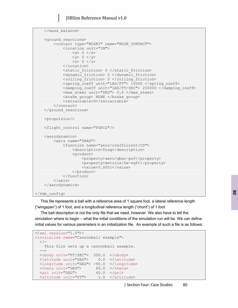
JSBSim Reference Manual v1.0
| Section Four: Case Studies 80
80
</mass_balance> <ground_reactions> <contact type="BOGEY" name="NOSE_CONTACT"> <location unit="IN"> <x> 0 </x> <y> 0 </y> <z> 0 </z> </location> <static_friction> 0 </static_friction> <dynamic_friction> 0 </dynamic_friction> <rolling_friction> 0 </rolling_friction> <spring_coeff unit="LBS/FT"> 10000 </spring_coeff> <damping_coeff unit="LBS/FT/SEC"> 200000 </damping_coeff> <max_steer unit="DEG"> 0.0 </max_steer> <brake_group> NONE </brake_group> <retractable>0</retractable> </contact> </ground_reactions> <propulsion/> <flight_control name="FGFCS"/> <aerodynamics> <axis name="DRAG"> <function name="aero/coefficient/CD"> <description>Drag</description> <product> <property>aero/qbar-psf</property> <property>metrics/Sw-sqft</property> <value>0.0001</value> </product> </function> </axis> </aerodynamics> </fdm_config>
This file represents a ball with a reference area of 1 square foot, a lateral reference length (“wingspan”) of 1 foot, and a longitudinal reference length (“chord”) of 1 foot.
The ball description is not the only file that we need, however. We also have to tell the simulation where to begin – what the initial conditions of the simulation run will be. We can define initial values for various parameters in an initialization file. An example of such a file is as follows:
<?xml version="1.0"?> <initialize name="Cannonball example"> <!— This file sets up a cannonball example. --> <ubody unit="FT/SEC"> 500.0 </ubody> <latitude unit="DEG"> 0.0 </latitude> <longitude unit="DEG"> -90.0 </longitude> <theta unit="DEG"> 60.0 </theta> <psi unit="DEG"> 40.0 </psi> <altitude unit="FT"> 1.0 </altitude>

JSBSim Reference Manual v1.0
| Section Four: Case Studies 81
81
</initialize>
The file above sets the ball up with an initial velocity of 500 feet per second along its own X axis, and an angle of 60 degrees above the horizon, at a heading of 40 degrees east of north. The initial location is on the equator at 90 degrees west longitude.
A simulation run can be made using this command line (assuming that the jsbsim executable is in your path):
jsbsim --aircraft=ball --initfile=cannonball_init
The “.xml” extension does not need to be given, nor should the full path to the files. The chart above shows the altitude versus time curve that results from this run.
0
500
1000
1500
2000
2500
3000
3500
0 5 10 15 20 25 30
Altitud
e (ft)
Time
Altitude vs. Time

JSBSim Reference Manual v1.0
| Section Four: Case Studies 82
82
3. Ball with parachute
We can go one step further over the previous example and add a parachute. This is made possible using the external reactions capability. The ball example is modified by adding the parachute as follows (see the external_reactions element):
<?xml version="1.0"?> <?xml-stylesheet type="text/xsl" href="http://jsbsim.sourceforge.net/JSBSim.xsl"?> <fdm_config name="BALL" version="2.0" release="BETA" xmlns:xsi=http://www.w3.org/2001/XMLSchema-instance xsi:noNamespaceSchemaLocation= "http://jsbsim.sourceforge.net/JSBSim.xsd"> <fileheader> <author> Jon Berndt </author> <filecreationdate> 2004-06-01 </filecreationdate> <version> Version 1.0 </version> <description> Test file </description> </fileheader> <metrics> <wingarea unit="FT2"> 1 </wingarea> <wingspan unit="FT"> 1 </wingspan> <chord unit="FT"> 1 </chord> <htailarea unit="FT2"> 0 </htailarea> <htailarm unit="FT"> 0 </htailarm> <vtailarea unit="FT2"> 0 </vtailarea> <vtailarm unit="FT"> 0 </vtailarm> <location name="AERORP" unit="IN"> <x> 0 </x> <y> 0 </y> <z> 0 </z> </location> </metrics> <mass_balance> <ixx unit="SLUG*FT2"> 10 </ixx> <iyy unit="SLUG*FT2"> 10 </iyy> <izz unit="SLUG*FT2"> 10 </izz> <emptywt unit="LBS"> 50 </emptywt> <location name="CG" unit="IN"> <x> 0 </x> <y> 0 </y> <z> 0 </z> </location> </mass_balance>

JSBSim Reference Manual v1.0
| Section Four: Case Studies 83
83
<ground_reactions> <contact type="BOGEY" name="CONTACT"> <location unit="IN"> <x> 0 </x> <y> 0 </y> <z> 0 </z> </location> <static_friction> 0 </static_friction> <dynamic_friction> 0 </dynamic_friction> <rolling_friction> 0 </rolling_friction> <spring_coeff unit="LBS/FT"> 10000 </spring_coeff> <damping_coeff unit="LBS/FT/SEC"> 200000 </damping_coeff> <max_steer unit="DEG"> 0.0 </max_steer> <brake_group> NONE </brake_group> <retractable>0</retractable> </contact> </ground_reactions> <external_reactions> <!— "Declare" the reefing term that will be set in the script. --> <property> fcs/parachute_reef_pos_norm </property> <force name="parachute" frame="WIND"> <function> <product> <property> aero/qbar-psf </property> <property> fcs/parachute_reef_pos_norm </property> <value> 1.0 </value> <!-- Full drag coefficient --> <value> 20.0 </value> <!-- Full parachute area --> </product> </function> <!— The location below is in structural frame (x positive aft), so this location describes a point 1 foot aft of the origin. In this case, the origin is the center. --> <location unit="FT"> <x>1</x> <y>0</y> <z>0</z> </location> <!— The direction describes a unit vector. In this case, since the selected frame is the WIND frame, the "-1" x component describes a direction exactly opposite of the direction into the wind vector. That is, the direction specified below is the direction that the drag force acts in.
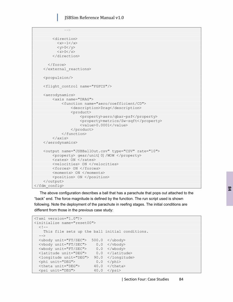
JSBSim Reference Manual v1.0
| Section Four: Case Studies 84
84
--> <direction> <x>-1</x> <y>0</y> <z>0</z> </direction> </force> </external_reactions> <propulsion/> <flight_control name="FGFCS"/> <aerodynamics> <axis name="DRAG"> <function name="aero/coefficient/CD"> <description>Drag</description> <product> <property>aero/qbar-psf</property> <property>metrics/Sw-sqft</property> <value>0.0001</value> </product> </function> </axis> </aerodynamics> <output name="JSBBallOut.csv" type="CSV" rate="10"> <property> gear/unit[0]/WOW </property> <rates> ON </rates> <velocities> ON </velocities> <forces> ON </forces> <moments> ON </moments> <position> ON </position> </output> </fdm_config>
The above configuration describes a ball that has a parachute that pops out attached to the “back” end. The force magnitude is defined by the function. The run script used is shown following. Note the deployment of the parachute in reefing stages. The initial conditions are different from those in the previous case study:
<?xml version="1.0"?> <initialize name="reset00"> <!-- This file sets up the ball initial conditions. --> <ubody unit="FT/SEC"> 500.0 </ubody> <vbody unit="FT/SEC"> 0.0 </vbody> <wbody unit="FT/SEC"> 0.0 </wbody> <latitude unit="DEG"> 0.0 </latitude> <longitude unit="DEG"> 90.0 </longitude> <phi unit="DEG"> 0.0 </phi> <theta unit="DEG"> 40.0 </theta> <psi unit="DEG"> 40.0 </psi>

JSBSim Reference Manual v1.0
| Section Four: Case Studies 85
85
<altitude unit="FT"> 10000.0 </altitude> <winddir unit="DEG"> 0.0 </winddir> <vwind unit="FT/SEC"> 0.0 </vwind> </initialize>
In words, the script below will,
• Deploy the parachute, reefed at 20%, when the ball descends below 5000 feet, • Disreef the parachute to 60% open when the ball descends below 4000 feet, • Disreef the parachute to 100% (fully open) when the ball descends below 2000 feet.
<?xml version="1.0" encoding="UTF-8"?> <?xml-stylesheet type="text/xsl" href="http://jsbsim.sf.net/JSBSimScript.xsl"?> <runscript xmlns:xsi=http://www.w3.org/2001/XMLSchema-instance xsi:noNamespaceSchemaLocation= "http://jsbsim.sf.net/JSBSimScript.xsd" name="ball test"> <description>Simplest of all tests</description> <use aircraft="ball" initialize="reset01"/> <run start="0.0" end="600" dt="0.008333"> <event name="Reef 1"> <description> Test of parachute reefing </description> <condition> <test> position/h-agl-ft lt 5000 </test> </condition> <set name="fcs/parachute_reef_pos_norm" value="0.2" action="FG_RAMP" tc="1.0"/> <notify> <property>sim-time-sec</property> </notify> </event> <event name="Reef 2"> <description> Test of parachute reefing </description> <condition> <test> position/h-agl-ft lt 4000 </test> </condition> <set name="fcs/parachute_reef_pos_norm" value="0.6" action="FG_RAMP" tc="1.0"/> <notify> <property>sim-time-sec</property> </notify> </event> <event name="Reef Final"> <description> Test of parachute reefing </description> <condition> <test>

JSBSim Reference Manual v1.0
| Section Four: Case Studies 86
86
position/h-agl-ft lt 2000 </test> </condition> <set name="fcs/parachute_reef_pos_norm" value="1.0" action="FG_RAMP" tc="1.0"/> <notify> <property>sim-time-sec</property> </notify> </event> <event name="Terminate"> <description> End condition </description> <condition> <test> gear/unit[0]/WOW eq 1 </test> </condition> <set name="simulation/terminate" value="1.0"/> <notify> <property>sim-time-sec</property> </notify> </event> </run> </runscript>
The plot of velocity and altitude versus time is shown:
0
100
200
300
400
500
600
700
800
0
2000
4000
6000
8000
10000
12000
14000
0 200 400 600 800 1000
Velocity (ft/sec)
Altitud
e (ft)
Time
Altitude and Velocity vs. Time
Altitude (ft)Velocity

JSBSim Reference Manual v1.0
| Section Four: Case Studies 87
87
4. Piston Aircraft with Autopilot and Scripting
For a more involved example, we’ll look at modeling a wing leveler autopilot and the flight control roll model for a small general aviation aircraft. Following that, we’ll also examine a heading hold autopilot. We’ll refer to this aircraft model as the c172x. The entire XML file that describes the c172x will not be shown here. See the JSBSim distribution for that.
4.1 An Automatic Wing Leveler We will assume that we have an aircraft model already at our disposal: the c172x, and that the
mass properties, aerodynamics, propulsion, etc. are already determined. We begin this case study by asking the question, how can we give the aircraft flight model the capability to hold a wings-level attitude during a scripted flight? We know that if we want to hold a roll attitude of zero (wings-level), we’ll have to generate a roll command that acts to remove the non-zero roll angle and return to wings-level flight. Such an autopilot will have to control the ailerons.
The autopilot control components can either go in the <autopilot> element in the aircraft configuration file, or they can be put in a separate file, which permits easier reuse. This time, we’ll put the component descriptions in the aircraft configuration file, in the <autopilot> element. The relevant part of the configuration file is as follows:
<autopilot name=”C172 A/P”> <channel name=”Roll”> … component definitions … </channel> </autopilot> <flight_control name=”C172 FCS”> <channel name=”roll”> … component definitions … </channel> </flight_control>
Let’s make one more assumption at this point: let’s assume that the normal roll flight control channel is already constructed, and that the inputs to the roll channel are:
• Roll trim • Roll command (from the pilot joystick) • Roll command (from the autopilot)
The “normal roll flight control” channel is the set of components that takes the above inputs (which range from -1 to +1 individually and as a sum total), processes the signal as needed, and

JSBSim Reference Manual v1.0
| Section Four: Case Studies 88
88
outputs an aileron command. We will use a PID controller to process the roll angle error and output an aileron command
that will keep the wings level. What is a PID controller? From Wikipedia: A proportional–integral–derivative controller (PID controller) is a generic control loop
feedback mechanism widely used in industrial control systems. A PID controller attempts to correct the error between a measured process variable and a desired setpoint by calculating and then outputting a corrective action that can adjust the process accordingly.
The PID controller calculation (algorithm) involves three separate parameters; the Proportional, the Integral and Derivative values. The Proportional value determines the reaction to the current error, the Integral determines the reaction based on the sum of recent errors and the Derivative determines the reaction to the rate at which the error has been changing. The weighted sum of these three actions is used to adjust the process via a control element such as the position of a control valve or the power supply of a heating element. A diagram of our wing leveler control law is shown below:
In JSBSim-ML, this looks like (with example gains thrown in):
<pid name="fcs/roll-ap-error-pid"> <input> attitude/phi-rad </input> <kp> 50.0 </kp> <ki> 5.0 </ki> <kd> 17.0 </kd> <output> ap/aileron_cmd </output> </pid>
It doesn’t get much simpler than this, does it? However, there is more that needs to be done. The autopilot of course is not going to be on at all times. And any time the PID controller is getting a non-zero input and the integrator gain is non-zero, the integrator output will be building up. So, it’s important to make sure that the integrator is properly used. We can modify the above controller to use a switch that controls the integrator state, and another switch to actually use the output.
This is a good place to explain the wind-up protection in the integrators that JSBSim provides in the flight control components. If a trigger property is specified via the <trigger> element in the PID control specification, the operation of the integrator is determined by the value of the property. If the value of the property is zero (actually, if the absolute value of the property is less that 0.000001) then the integrator operates normally. If the value of the trigger property is
Kp
Ki∫e(t)
Kdė(t)
PID Controller
Roll angle (rad) Aileron command (rad)
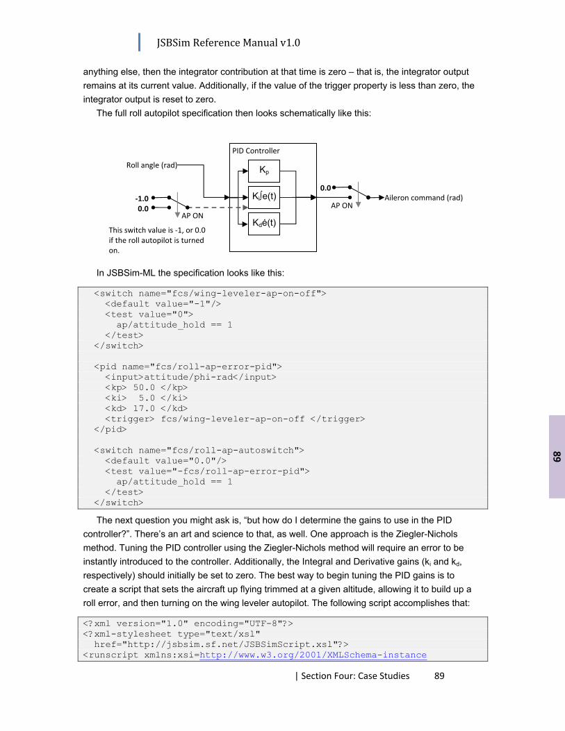
JSBSim Reference Manual v1.0
| Section Four: Case Studies 89
89
anything else, then the integrator contribution at that time is zero – that is, the integrator output remains at its current value. Additionally, if the value of the trigger property is less than zero, the integrator output is reset to zero.
The full roll autopilot specification then looks schematically like this:
In JSBSim-ML the specification looks like this:
<switch name="fcs/wing-leveler-ap-on-off"> <default value="-1"/> <test value="0"> ap/attitude_hold == 1 </test> </switch> <pid name="fcs/roll-ap-error-pid"> <input>attitude/phi-rad</input> <kp> 50.0 </kp> <ki> 5.0 </ki> <kd> 17.0 </kd> <trigger> fcs/wing-leveler-ap-on-off </trigger> </pid> <switch name="fcs/roll-ap-autoswitch"> <default value="0.0"/> <test value="-fcs/roll-ap-error-pid"> ap/attitude_hold == 1 </test> </switch>
The next question you might ask is, “but how do I determine the gains to use in the PID controller?”. There’s an art and science to that, as well. One approach is the Ziegler-Nichols method. Tuning the PID controller using the Ziegler-Nichols method will require an error to be instantly introduced to the controller. Additionally, the Integral and Derivative gains (ki and kd, respectively) should initially be set to zero. The best way to begin tuning the PID gains is to create a script that sets the aircraft up flying trimmed at a given altitude, allowing it to build up a roll error, and then turning on the wing leveler autopilot. The following script accomplishes that:
<?xml version="1.0" encoding="UTF-8"?> <?xml-stylesheet type="text/xsl" href="http://jsbsim.sf.net/JSBSimScript.xsl"?> <runscript xmlns:xsi=http://www.w3.org/2001/XMLSchema-instance
AP ON AP ON
0.0
Kp
Ki∫e(t)
Kdė(t)
PID Controller
Roll angle (rad)
Aileron command (rad) ‐1.0 0.0
This switch value is ‐1, or 0.0 if the roll autopilot is turned on.

JSBSim Reference Manual v1.0
| Section Four: Case Studies 90
90
xsi:noNamespaceSchemaLocation=http://jsbsim.sf.net/JSBSimScript.xsd name="At-altitude autopilot test setup."> <use aircraft="c172x" initialize="reset01"/> <run start="0.0" end="30" dt="0.00833333"> <!-- Start the engine --> <event name="Engine start"> <condition>sim-time-sec ge 0.25</condition> <set name="fcs/throttle-cmd-norm" value="0.65"/> <set name="fcs/mixture-cmd-norm" value="0.87"/> <set name="propulsion/magneto_cmd" value="3"/> <set name="propulsion/starter_cmd" value="1"/> <set name="ap/heading_hold" value="0"/> <notify> <property>velocities/vc-kts</property> <property>position/h-agl-ft</property> </notify> </event> <!—Trim the aircraft --> <event name="Trim"> <condition>sim-time-sec ge 0.50</condition> <set name="simulation/do_simple_trim" value="0"/> <notify> <property>velocities/vc-kts</property> <property>position/h-agl-ft</property> </notify> </event> <!-- Turn on the roll autopilot after a roll “error” has developed (5 seconds) --> <event name="Set roll autopilot"> <condition>sim-time-sec ge 5.0</condition> <set name="ap/attitude_hold" value="1"/> <notify> <property>velocities/vc-kts</property> <property>position/h-agl-ft</property> </notify> </event> </run> </runscript>
Running JSBSim with this script, then plotting the roll angle versus time will show how the PID controller is working to reduce the roll angle error. The Ziegler-Nichols method can be employed as follows:
1) Make repeated runs, increasing the proportional gain Kp until the control action is seen to cause a sustained oscillatory control output. That gain is referred to as the ultimate gain, Ku, or the critical gain. Note also the peak-to-peak period of the oscillation. That is referred to as the critical oscillation period, Tc.
2) Knowing Kc and Tc, the PID gains can be set depending on whether a P, PI, or PID controller is needed. The gains are set according to the following table:

JSBSim Reference Manual v1.0
| Section Four: Case Studies 91
91
Control Type Kp Ki Kd
P 0.5 Kc 0 0
PI 0.45 Kc 1.2Kp/Tc 0
PID 0.6 Kc 2 Kp/Tc KpTc/8
Let’s walk through this. A series of ten runs will be made with the integrator and derivative
gains set to zero. The proportional gain will be set to 5 initially and increased by five for each subsequent run. This process is carried out with a shell script that runs JSBSim repeatedly, with gain values specified on the command line. First, the PID controller is modified to have its gains specified as properties. This allows the gains to be set somewhere else (such as from a script):
<autopilot name="C-172X Autopilot"> <!-- INTERFACE PROPERTIES --> … <!-- INITIAL GAIN VALUES --> <property value="50.0"> ap/roll-pid-kp </property> <property value="5.0"> ap/roll-pid-ki </property> <property value="17.0"> ap/roll-pid-kd </property> … <channel name="Roll wing leveler"> … <pid name="fcs/roll-ap-error-pid"> <input>attitude/phi-rad</input> <kp> ap/roll-pid-kp </kp> <ki> ap/roll-pid-ki </ki> <kd> ap/roll-pid-kd </kd> <trigger> fcs/wing-leveler-ap-on-off </trigger> </pid>
The shell script that makes the multiple runs is,
src/jsbsim --script=scripts/c1722 \ --property=ap/roll-pid-kp=5 \ --property=ap/roll-pid-ki=0 \ --property=ap/roll-pid-kd=0 \ --logdirectivefile=output.xml \ --outputlogfile=pid_test_0.csv … src/jsbsim --script=scripts/c1722 \ --property=ap/roll-pid-kp=50 \ --property=ap/roll-pid-ki=0 \ --property=ap/roll-pid-kd=0 \ --logdirectivefile=output.xml \ --outputlogfile=pid_test_9.csv
This shell script also shows that JSBSim is being told to take the output specification from the

JSBSim Reference Manual v1.0
| Section Four: Case Studies 92
92
file output.xml. That file contains a property element, directing the program to output only roll angle in radians (attitude/phi-rad). The logged output data itself is sent to the named file, pid_test_#.csv, where “#” represents a number from 0 to 9.
When all the data is plotted together, the response to the different value of Kp is seen. The plot begins the same for all cases: the aircraft begins flying at altitude, and begins a slow roll to the left (left wingtip down). The controller is turned on at five seconds.
From the plot above, one can determine that the system response began to oscillate when the
gain Kp was set to 50 – this is Kc – the critical gain. The peak-to-peak period of the oscillation is 0.667 seconds – this is Tc. Given the gain chart shown in step 2 of the Ziegler-Nichols method description, if a proportional only control is used, the gain Kp should be set to 0.5 Kc, or, 25. If we make the same run using that arrangement, the roll angle behavior looks like that shown in the plot:

JSBSim Reference Manual v1.0
| Section Four: Case Studies 93
93
The plot shows the roll angle being corrected, but with significant overshoot and a steady state error. So, let’s try to use PI control and eliminate the bias. Again referring to the Ziegler-Nichols chart from step 2, we get a value for Kp of 22.5 and so the value for Ki is calculated from that to be 1.2 Kp/Tc = 40.48. When we run the simulation with this setup, we get this roll angle behavior:

JSBSim Reference Manual v1.0
| Section Four: Case Studies 94
94
The roll angle action is more oscillatory, but the steady state error is about zero. Let’s try adding derivative control, to make a full PID controller, and see if that helps. Looking at the third line in the Ziegler-Nichols chart, we calculate the gains as follows: Kp = 0.6 Kc = 30, Ki = 2 Kp/Tc = 90, Kd = Kp Tc/8 = 2.5. Making a run with these values results in this roll angle behavior:

JSBSim Reference Manual v1.0
| Section Four: Case Studies 95
95
There is significant overshoot here, too, but it’s less than before, and the oscillation is gone. The roll angle snaps to the wings-level position very rapidly – perhaps too rapidly! We might like to try and reduce the overshoot. But, which gain or gains do we adjust? Here’s a table that shows the response to increasing any of the gains on the controller output:
Effects of increasing parameters
Parameter Rise Time Overshoot Settling Time S.S. Error
Kp Decrease Increase Small Change Decrease
Ki Decrease Increase Increase Eliminate
Kd Small Decrease Decrease Decrease None
From the chart above, it looks like we might want to increase the derivative gain, which would decrease the overshoot and the settling time. After some additional tweaking, we arrive at gains, Kp=50, Ki=6, Kd=18. The plot of the response (roll angle) to the controller is shown below:
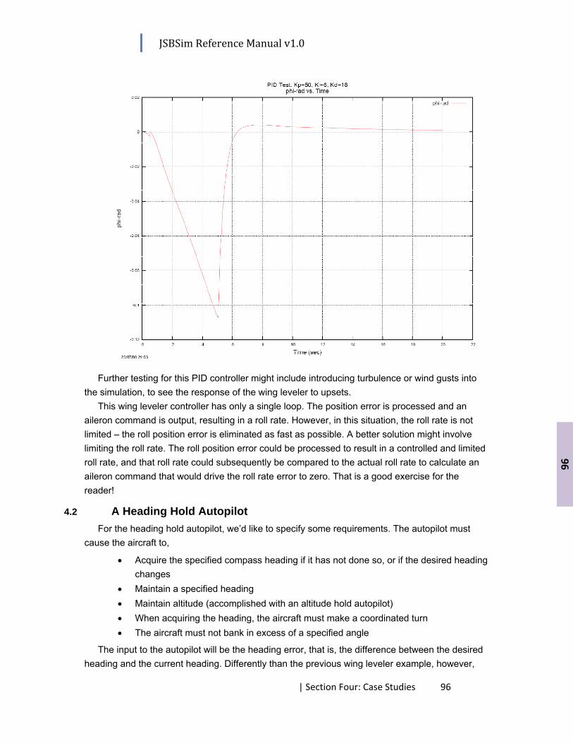
JSBSim Reference Manual v1.0
| Section Four: Case Studies 96
96
Further testing for this PID controller might include introducing turbulence or wind gusts into
the simulation, to see the response of the wing leveler to upsets. This wing leveler controller has only a single loop. The position error is processed and an
aileron command is output, resulting in a roll rate. However, in this situation, the roll rate is not limited – the roll position error is eliminated as fast as possible. A better solution might involve limiting the roll rate. The roll position error could be processed to result in a controlled and limited roll rate, and that roll rate could subsequently be compared to the actual roll rate to calculate an aileron command that would drive the roll rate error to zero. That is a good exercise for the reader!
4.2 A Heading Hold Autopilot For the heading hold autopilot, we’d like to specify some requirements. The autopilot must
cause the aircraft to,
• Acquire the specified compass heading if it has not done so, or if the desired heading changes
• Maintain a specified heading • Maintain altitude (accomplished with an altitude hold autopilot) • When acquiring the heading, the aircraft must make a coordinated turn • The aircraft must not bank in excess of a specified angle
The input to the autopilot will be the heading error, that is, the difference between the desired heading and the current heading. Differently than the previous wing leveler example, however,

JSBSim Reference Manual v1.0
| Section Four: Case Studies 97
97
the error will not be fed into a PID controller and directly result in a control surface command, but will instead be turned into a roll position command. The roll position command will be compared with the current bank angle and the difference (the error) will then be fed into another PID controller, and the output from that controller will be a roll rate command – which will be accomplished using the ailerons. In words, if there is a heading error, let’s roll towards the desired heading, but let’s keep our roll rate below a specified limit and keep the bank at an angle no greater than 30 degrees. Schematically, our heading hold autopilot will look like this:
ψdesired
ψactual
Kp
Ki∫e(t)
Kdė(t)
PID Controller
Heading error calc.
Limiter
φactual
Kp
Ki∫e(t)
Kdė(t)
PID Controller
Limiter
-
Heading Error Roll Position
δa,cmd
Kp
Ki∫e(t)
Kdė(t)
PID Controller
Roll Rate
Limiter
-
pactual
JSBSim Reference Manual v1.0
| Section Four: Case Studies 98
98
5. Modeling a Waypoint Navigation System
The flight control model in JSBSim is completely configurable and includes many components that can be strung together to model specific control laws. Various automatic flight capabilities have already been modeled for some aircraft to help with testing the aircraft outside of FlightGear or other simulator. The C-172x model in the JSBSim distribution has an attitude hold, altitude hold, and heading hold capability built up.
A specific capability is needed for this case study: a waypoint navigation system (WNS) that would allow a user to enter latitude and longitude coordinates (in radians) that the aircraft would then fly to. An algorithm is developed based on the Haversine forumulas ,
Haversine Formulas R = Earth radius (5.1) Δlat = lat2 – lat1 (5.2) Δlong = long2 – long1 (5.3) a = sin2(Δlat/2) + cos(lat1)·cos(lat2)·sin2(Δlong/2) (5.4) c = 2·atan2(√a, √(1−a)) (5.5) distance = R·c (5.6) Φ = atan2( sin(Δlong)·cos(lat2), cos(lat1)·sin(lat2) − sin(lat1) ·cos(lat2)·cos(Δlong) ) (5.7)
There does exist a file in the C310 directory in the default JSBSim CVS release that includes a modified version of the autopilot functions developed for testing the C172x aircraft model. The C310ap.xml file contains a heading hold, wing leveler, and altitude-hold functionality. Since the WNS calculates a heading that should be flown to, it can supply the existing heading hold autopilot with the correct heading – that is, it can feed a heading hold sub-mode. This is our assumed starting point.
The first task we will take on will be to add a set of calculations in the C310ap.xml file that will calculate the heading to a specified waypoint. First, some preliminary calculations will need to be made: delta latitude, and delta longitude. These are defined in JSBSim-ML as seen in Listing 5.1, below:
Listing 5.1 <fcs_function name="fcs/delta-lat-rad"> <!-- Delta latitude in radians --> <function> <difference> <property>ap/wp_latitude_rad</property> <property>position/lat-gc-rad</property> </difference> </function> </fcs_function>

JSBSim Reference Manual v1.0
| Section Four: Case Studies 99
99
<fcs_function name="fcs/delta-lon-rad"> <!-- Delta longitude in radians --> <function> <difference> <property>ap/wp_longitude_rad</property> <property>position/long-gc-rad</property> </difference> </function> </fcs_function>
The JSBSim properties for geocentric latitude and longitude are:
• position/lat-gc-rad • position/long-gc-rad
The properties for desired latitude and longitude (the waypoint) are:
• ap/wp_latitude_rad • ap/wp_longitude_rad
The function definitions above result in the creation of new properties at runtime, representing the difference between the desired position and the actual position. The automatically generated properties that represent the output of the calculations above are:
• fcs/delta-lon-rad • fcs/delta-lat-rad
The above two property values represent equations 5.2 and 5.3. The actual heading from the current position to the desired location (specified by the waypoint) is given by the solution to equation 5.7. In JSBSim-ML, the definition looks like that given in Listing 5.2,
Listing 5.2 <fcs_function name="fcs/heading-to-waypoint-rad"> <function> <atan2> <!-- atan2 (deltaY, deltaX )--> <product> <sin><property>fcs/delta-lon-rad</property></sin> <cos><property>ap/wp_latitude_rad</property></cos> </product> <difference> <product> <cos><property>position/lat-gc-rad</property></cos> <sin><property>ap/wp_latitude_rad</property></sin> </product> <product> <sin><property>position/lat-gc-rad</property></sin> <cos><property>ap/wp_latitude_rad</property></cos> <cos><property>fcs/delta-lon-rad</property></cos> </product> </difference> </atan2> </function> </fcs_function>
The next task is to calculate the distance to the waypoint from the current position. There are
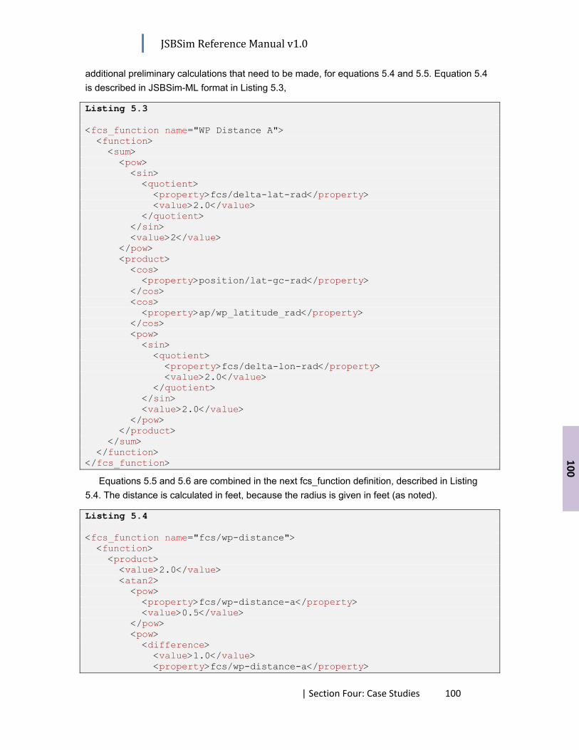
JSBSim Reference Manual v1.0
| Section Four: Case Studies 100
100
additional preliminary calculations that need to be made, for equations 5.4 and 5.5. Equation 5.4 is described in JSBSim-ML format in Listing 5.3,
Listing 5.3 <fcs_function name="WP Distance A"> <function> <sum> <pow> <sin> <quotient> <property>fcs/delta-lat-rad</property> <value>2.0</value> </quotient> </sin> <value>2</value> </pow> <product> <cos> <property>position/lat-gc-rad</property> </cos> <cos> <property>ap/wp_latitude_rad</property> </cos> <pow> <sin> <quotient> <property>fcs/delta-lon-rad</property> <value>2.0</value> </quotient> </sin> <value>2.0</value> </pow> </product> </sum> </function> </fcs_function>
Equations 5.5 and 5.6 are combined in the next fcs_function definition, described in Listing 5.4. The distance is calculated in feet, because the radius is given in feet (as noted).
Listing 5.4 <fcs_function name="fcs/wp-distance"> <function> <product> <value>2.0</value> <atan2> <pow> <property>fcs/wp-distance-a</property> <value>0.5</value> </pow> <pow> <difference> <value>1.0</value> <property>fcs/wp-distance-a</property>

JSBSim Reference Manual v1.0
| Section Four: Case Studies 101
101
</difference> <value>0.5</value> </pow> </atan2> <!-- 21144000 is the Earth’s radius in feet --> <value>21144000</value> </product> </function> </fcs_function>
Finally, there are three remaining short component definitions that need to be added to complete the WNS (see Listing 5.5). The summer component adds 2*pi to the heading command computed by the function component presented in Listing 2, for possible use in the next step. The switch component that follows the function component includes a conditional test of the heading-to-waypoint-rad command. If the heading-to-waypoint-rad value is already positive, then the switch takes as its output value the value specified by the heading-to-waypoint-rad property. Otherwise, the switch takes on the default value specified in the switch, heading-to-waypoint-positive, calculated previously in the summer component. Thus, the output from the switch is a positive heading command in radians. The last of these three components takes as input the switch output calculated just previously, and multiplies it by 57.3, thus turning it into a heading command in degrees.
Listing 5.5 <summer name="fcs/heading-to-waypoint-positive"> <input> fcs/heading-to-waypoint-rad </input> <bias> 6.283 </bias> </summer> <switch name="fcs/wp-heading-corrector"> <default value="fcs/heading-to-waypoint-positive"/> <test value="fcs/heading-to-waypoint-rad"> fcs/heading-to-waypoint-rad gt 0.0 </test> </switch> <pure_gain name="fcs/wp-heading-deg"> <input> fcs/wp-heading-corrector </input> <gain> 57.3 </gain> </pure_gain>
The heading command can be fed into the previously developed heading autopilot. So, the heading autopilot can now actually take either a direct heading command, or the command calculated from the WNS.
At this point we’d like to consider testing. The test involves the creation of a script to set waypoints, and a way to display the results to verify that the performance is as expected.
The test script is written in XML format. The basic format of a JSBSim script is:
<use aircraft=“name” initialize=“file”/> <run start=“0” end=“time” dt=“0.0833”> <event>

JSBSim Reference Manual v1.0
| Section Four: Case Studies 102
102
… condition[s] … … action[s] … </event> … more events … </run>
In this test, we need to do several things:
1. Start the engines. 2. Set the autopilot mode to “heading hold”. 3. Set the initial waypoint latitude and longitude. 4. Set the initial target altitude. 5. Activate the altitude autopilot on cue. 6. Raise the landing gear on cue. 7. Head to the first waypoint on cue. 8. Head to subsequent waypoints on cue. 9. Terminate on cue.
The script directs the actions as expected, but there is one feature of scripting that needs to be considered carefully: order of execution. Inputs to the script are calculated once per frame, so each test will see the same input value. For instance, prior to evaluating the tests for each event, inputs will have been calculated (such as current latitude, or the distance to a waypoint). Each property that is set in an event will take effect immediately (such as for active_waypoint). Since events are stored in program memory sequentially as they are found in the script file—and since they are likewise executed sequentially—it is possible for carelessly crafted sequential events to have their conditions evaluate to true in a single frame, in effect experiencing a cascading sequential execution. In this script, that could happen when a waypoint is reached and an event is triggered due to proximity to the target waypoint. The action taken in this test script when a waypoint is reached is to set the active waypoint to the index of the next waypoint. But, when the next waypoint test is evaluated, the distance value previously calculated may be less than the threshold distance specified for the next waypoint. With the active waypoint set to the next waypoint, the test will immediately be triggered. Subsequent events may also be triggered immediately. The solution is to list the affected events in reverse order in the script file. What happens in this case is that events which evaluate to true are followed by events that have already been triggered and executed.
The script specifies that the C310.xml file should be used. We also need to provide an initialization file that describes where to start the flight, and the initial orientation, etc. Since I am familiar with the area, Ellington Field near Houston, Texas was selected as the starting point for the scripted test flight.
Using the Google Earth application (which can be downloaded freely at http://earth.google.com) I inspected the region and picked out a few locations through which I wanted the aircraft to fly. The initial point, however, is the important one for the initialization file, representing Ellington field. The additional points are on the approach to one of the runways at Houston Hobby Airport, past that same runway, at the southwest end of Galveston Island, and at the northeast end of Galveston Island.

JSBSim Reference Manual v1.0
| Section Four: Case Studies 103
103
The script that performs the test is as follows:
<?xml version="1.0" encoding="UTF-8"?> <?xml-stylesheet type="text/xsl" href="http://jsbsim.sf.net/JSBSimScript.xsl"?> <runscript xmlns:xsi=http://www.w3.org/2001/XMLSchema-instance xsi:noNamespaceSchemaLocation=http://jsbsim.sf.net/JSBSimScript.xsd name="C310-01A takeoff run"> <description>For testing autopilot capability</description> <use aircraft="c310" initialize="Ellington"/> <run start="0.0" end="3600" dt="0.00833333"> <event name="Start engine"> <description> Start engine and set initial heading and waypoints, turn on heading-hold mode. </description> <condition>sim-time-sec ge 0.25</condition> <set name="fcs/mixture-cmd-norm[0]" value="0.87"/> <set name="fcs/mixture-cmd-norm[1]" value="0.87"/> <set name="fcs/advance-cmd-norm[0]" value="1.0"/> <set name="fcs/advance-cmd-norm[1]" value="1.0"/> <set name="propulsion/magneto_cmd" value="3"/> <set name="fcs/throttle-cmd-norm[0]" value="1.0"/> <set name="fcs/throttle-cmd-norm[1]" value="1.0"/> <set name="propulsion/starter_cmd" value="1"/> <set name="ap/altitude_setpoint" action="FG_EXP" value="1000" tc="10"/> <set name="ap/attitude_hold" value="0"/> <set name="ap/wp_latitude_rad" value="0.517238"/> <set name="ap/wp_longitude_rad" value="-1.662727"/> <set name="ap/heading_setpoint" value="355"/> <set name="ap/heading-setpoint-select" value="0"/> <set name="ap/heading_hold" value="1"/> <set name="ap/active-waypoint" value="0"/> <notify/> </event> <event name="Set altitude for 1,000 ft."> <condition>velocities/vc-fps ge 135.0</condition> <set name="ap/altitude_hold" value="1"/> <notify/> </event> <event name="Raise landing gear"> <condition>position/h-agl-ft ge 20</condition> <set name="gear/gear-cmd-norm" value="0"/> <notify/> </event> <event name="Head to first waypoint"> <description> Set heading hold to selected waypoint (setpoint) instead of previously specified heading when altitude surpasses 800 feet. </description>

JSBSim Reference Manual v1.0
| Section Four: Case Studies 104
104
<condition>position/h-agl-ft ge 800</condition> <set name="ap/heading-setpoint-select" value="1"/> <set name="ap/active-waypoint" value="1"/> <notify> <property>fcs/wp-distance</property> </notify> </event> <event name="Terminate"> <description> When the aircraft arrives back at Ellington Field (fifth waypoint) then terminate the simulation. </description> <condition> fcs/wp-distance lt 100 ap/active-waypoint eq 5 </condition> <set name="simulation/terminate" value="1"/> <notify/> </event> <event name="Set last waypoint"> <description> When the distance to the fourth waypoint (northeast end of Galveston Island) is less than 100 feet, then set the last waypoint (back to Ellington Field). </description> <condition> fcs/wp-distance lt 100 ap/active-waypoint eq 4 </condition> <set name="ap/wp_latitude_rad" value="0.516512"/> <set name="ap/wp_longitude_rad" value="-1.660922"/> <set name="ap/active-waypoint" value="5"/> <notify> <property>fcs/wp-distance</property> </notify> </event> <event name="Set fourth waypoint"> <description> When the distance to the third waypoint (southwest end of Galveston Island) is less than 800 feet, then set the fourth waypoint (northeast end of Galveston Island). </description> <condition> fcs/wp-distance lt 800 ap/active-waypoint eq 3 </condition> <set name="ap/wp_latitude_rad" value="0.511661"/> <set name="ap/wp_longitude_rad" value="-1.653510"/> <set name="ap/active-waypoint" value="4"/> <notify> <property>fcs/wp-distance</property> </notify> </event>

JSBSim Reference Manual v1.0
| Section Four: Case Studies 105
105
<event name="Set third waypoint"> <description> When the distance to the second waypoint (Hobby Airport) is less than 300 feet, then set the third waypoint. </description> <condition> fcs/wp-distance lt 300 ap/active-waypoint eq 2 </condition> <set name="ap/wp_latitude_rad" value="0.507481"/> <set name="ap/wp_longitude_rad" value="-1.660062"/> <set name="ap/active-waypoint" value="3"/> <notify> <property>fcs/wp-distance</property> </notify> </event> <event name="Set second waypoint"> <description> When the distance to the first waypoint (Hobby Airport threshold) is less than 700 feet, then set the second waypoint. </description> <condition> fcs/wp-distance lt 700 ap/active-waypoint eq 1 </condition> <set name="ap/wp_latitude_rad" value="0.517533"/> <set name="ap/wp_longitude_rad" value="-1.663076"/> <set name="ap/active-waypoint" value="2"/> <notify> <property>fcs/wp-distance</property> </notify> </event> </run> </runscript>
[Article in-work … ]
JSBSim Reference Manual v1.0
| Section Four: Case Studies 106
106
6. Rocket with GNC and Scripting
For a long time now, rocket-propelled flight models in JSBSim have been possible (the X-15 was the first vehicle modeled for JSBSim), but in actually making a vertical, guided, rocket flight model, some new capabilities were added to support rocket flight. This section will cover some of the techniques used in executing rocket flight in JSBSim.
Some of the major differences in modeling vertical rocket flight (compared to modeling aircraft) are:
• Takeoff is vertical; ground reactions are tougher because they are stiffer. • Guidance in first stage (often corresponding roughly to the atmospheric flight phase)
is typically open loop, with second stage flight following a more complicated guidance scheme such as “Powered Explicit Guidance” (PEG).
• Control involves gimbaled effectors (thrusters, or nozzles). • Control is normally completely automatic. • Aerodynamic modeling is different. • Sensor modeling can be more complicated, since sensors such as accelerometers
cannot necessarily be placed at the center of mass (which may be inside a propellant tank!)
At this time, it is easy to model single stage rocket flight using JSBSim, but multi-stage flight is more cumbersome.
6.1 Addressing the ground reactions For a vertically launched rocket, a way was needed to keep the vehicle firmly attached to one
spot, as if it was mounted on a launch platform. It was not easy to make the standard ground reactions work well, particularly after the engines had been started, but before thrust had built up to the point where the vehicle lifted off the platform. So, a new flag was created (a property) which, if set, causes a ground reaction force equal and opposite to the aerodynamic, gravitational, and propulsive forces, and so the vehicle stays put. The property name for the hold-down flag is forces/hold-down.
6.2 Simple rocket guidance The path a rocket takes in vertical flight is not normally manually flown, because the total
angle of attack must be kept low to keep structural loads small, and to minimize aerodynamic drag. One key measurement tracked is q*alpha – that is, dynamic pressure multiplied by the angle of attack.
There are several phases of flight for a rocket ascending:
• The vertical rise phase • The kick angle or tilt phase
JSBSim Reference Manual v1.0
| Section Four: Case Studies 107
107
• The gravity turn phase
During the vertical rise period, the vehicle ascends straight up to clear the launch platform and then rolls to the alight to the appropriate heading. Sometimes, as it was in the case of the Apollo Saturn V, a slight yaw is introduced away from the launch tower just after liftoff. In the kick angle phase, the vehicle is commanded to an initial pitch angle, after which it begins the zero-lift (zero-alpha) gravity turn phase as it flies through the lower, most dense portion of the atmosphere at an increasingly higher velocity. Control during these phases is normally exercised by gimballing the main rocket engines, and/or through the use of auxiliary reaction control jets (RCS).
In JSBSim, we encounter a few new situations that must be addressed when modeling vertical rocket flight. First of all, in the vertical rise period, the question can be asked: how do we command the vehicle to roll to the appropriate heading, since the vehicle is pointed vertically? The frames of interest here are the local frame, which is a frame that is always underneath the aircraft, with the X axis pointing north, the Y axis pointing East, and the Z axis pointing downward. The origin of the local frame is at sea level. The vehicle body frame has the X axis along the vehicle centerline pointing forward out the nose, the Y axis pointing out the “right”, and the Z axis pointing “down” out the bottom of the vehicle. For a rocket, the Y and Z directions seem somewhat arbitrary. Placing the rocket initially on a launch pad at Kennedy Space Center, Kourou, or Baikonur (for example), involves setting the initial latitude, longitude, and altitude, and orienting the vehicle on the launch pad. Since the order of rotations used in JSBSim to describe the orientation of a vehicle (that is, the orientation of the body frame for the vehicle) relative to the local frame is yaw, then pitch, then roll, it can be seen that the vehicle orientation can be described as having a pitch angle of +90 degrees relative to the local frame. If the vehicle has a particular roll orientation on the pad, the vehicle can be rolled after it is initially pitched. The initial orientation can be specified in the initialization file as having a particular psi, theta, and phi (Euler angles).
During the vertical rise period, the vehicle is pointed nearly straight upwards, which can cause problems in any guidance we might use to keep the vehicle pointed straight up, and also to roll it to a particular heading. One way to get around this is to simply devise a controller that both keeps the pitch and yaw rates at zero (which keeps the vehicle pointed up), and commands a roll rate to achieve the desired heading once the pitchover begins. The roll rate needs to be carefully controlled to ramp up, then back down to zero, prior to beginning to pitch over.
Control of the vehicle is performed (as mentioned before) by gimballing engines (for pitch and yaw) or using RCS jets (for roll). For the vertical rise period, it is not too hard to set up a control law for the pitch and yaw axes that take the pitch (or yaw) rate as input and generates a pitch (or yaw) engine gimbal command to counter that and bring the respective rate back to zero.
6.3 “Moding” and Timing A question can be addressed at this time regarding how to command the various portions of
the flight – that is, when should the vertical rise, or the tilt, or the gravity turn phases be initiated? This is related in a way to the subject of how to organize the guidance, navigation, and control (referred to as GNC) aspects of a simulated rocket in JSBSim. We could call this the simulated “flight software” (FSW), which is really what is being represented. The question to address can be summed up: is the timing of the mode changes during the flight controlled from the ground (which
JSBSim Reference Manual v1.0
| Section Four: Case Studies 108
108
might be modeled in a script), or onboard the launch vehicle? If it originates on the launch vehicle, we might assert that the timing is part of the flight software. The various modes are then, in fact, initiated from aboard the vehicle itself. It’s the safest approach; think of what would happen in the case of a momentary communications loss.
So, for first stage flight we need a vertical rise phase, followed by a tilt phase, followed by a gravity turn phase – all controlled from the launch vehicle itself. For JSBSim that means we need the sequencing function to be present in the flight control or system section of the vehicle configuration file.
The system section is new in the latest version of JSBSim. Any number of systems can be defined, and they use the same syntax as the flight control section. The system section is useful when a guidance, or navigation, or electrical system is desired to be modeled in JSBSim using the suite of system components.
6.4 Where to Start? As with all JSBSim aircraft models, vehicle characteristics will need to be known:
• Mass properties • Geometry • Control • Propulsion • Aerodynamics • Ground contacts
Geometry is almost always quite easy. Mass properties are little bit harder, but one can make fairly good guesses at this. [Note: for some historic rockets such as the Saturn V or Saturn IB, there may be reference material available on the web and/or in technical papers.] Fuel burn-off might be a complicating factor because the CG may shift, there may be fuel slosh (for liquid propellant rockets), and moments of inertia will change. Control (Guidance, Navigation, and Control, actually) is the most involved part of modeling a rocket, I think. Propulsion for rockets can be modeled rather simply in JSBSim. Aerodynamics is second to control as far as level of difficulty. Ground contacts are straightforward.
6.5 Aerodynamics Let’s look at aerodynamics first. We can determine the aerodynamic characteristics of a
simple axisymmetric body using DATCOM+ (see www.holycows.net), or – if you have access to it – Missile DATCOM. There are other software titles out there as well. We will use the lift and drag curves for the V-2 missile (as found in Sutton’s Rocket Propulsion Elements book) to model our example rocket. We will also assume that the aerodynamics will be completely modeled by proper placement of the aerodynamic center of pressure, coupled with the lift and drag curves, and that the side force is the same as the lift force.
6.6 Mass Properties Since we know the mass characteristics of the Little Joe, we will scale the moments and
products of inertia of that vehicle once we specify the weight of our example rocket.

JSBSim Reference Manual v1.0
| Section Four: Case Studies 109
109
[Article in-work … ]

JJSBSim Refeerence Manu
Appe
ual v1.0
endic
| Ap
ces
ppendices 110
110

JSBSim Reference Manual v1.0
| Appendices 111
111
Native properties accelerations/Nz accelerations/a-pilot-x-ft_sec2 accelerations/a-pilot-y-ft_sec2 accelerations/a-pilot-z-ft_sec2 accelerations/n-pilot-x-norm accelerations/n-pilot-y-norm accelerations/n-pilot-z-norm accelerations/pdot-rad_sec2 accelerations/qdot-rad_sec2 accelerations/rdot-rad_sec2 accelerations/udot-ft_sec2 accelerations/vdot-ft_sec2 accelerations/wdot-ft_sec2 aero/alpha-deg aero/alpha-max-rad aero/alpha-min-rad aero/alpha-rad aero/alpha-wing-rad aero/alphadot-deg_sec aero/alphadot-rad_sec aero/beta-deg aero/beta-rad aero/betadot-deg_sec aero/betadot-rad_sec aero/bi2vel aero/ci2vel aero/cl-squared aero/h_b-cg-ft aero/h_b-mac-ft aero/mag-beta-deg aero/mag-beta-rad aero/qbar-area aero/qbar-psf aero/qbarUV-psf aero/qbarUW-psf aero/stall-hyst-norm atmosphere/P-psf
atmosphere/P-sl-psf atmosphere/T-R atmosphere/T-sl-R atmosphere/T-sl-dev-F atmosphere/a-fps atmosphere/a-ratio atmosphere/a-sl-fps atmosphere/crosswind-fps atmosphere/delta atmosphere/delta-T atmosphere/density-altitude atmosphere/gust-down-fps atmosphere/gust-east-fps atmosphere/gust-north-fps atmosphere/headwind-fps atmosphere/p-turb-rad_sec atmosphere/psiw-rad atmosphere/q-turb-rad_sec atmosphere/r-turb-rad_sec atmosphere/rho-sl-slugs_ft3 atmosphere/rho-slugs_ft3 atmosphere/sigma atmosphere/theta atmosphere/turb-gain atmosphere/turb-rate atmosphere/turb-rhythmicity atmosphere/wind-from-cw attitude/heading-true-rad attitude/phi-rad attitude/pitch-rad attitude/psi-rad attitude/roll-rad attitude/theta-rad fcs/aileron-cmd-norm fcs/center-brake-cmd-norm fcs/elevator-cmd-norm fcs/elevator-pos-deg

JSBSim Reference Manual v1.0
| Appendices 112
112
fcs/elevator-pos-norm fcs/elevator-pos-rad fcs/flap-cmd-norm fcs/flap-pos-deg fcs/flap-pos-norm fcs/flap-pos-rad fcs/left-aileron-pos-deg fcs/left-aileron-pos-norm fcs/left-aileron-pos-rad fcs/left-brake-cmd-norm fcs/mag-elevator-pos-rad fcs/mag-left-aileron-pos-rad fcs/mag-right-aileron-pos-rad fcs/mag-rudder-pos-rad fcs/mag-speedbrake-pos-rad fcs/mag-spoiler-pos-rad fcs/pitch-trim-cmd-norm fcs/right-aileron-pos-deg fcs/right-aileron-pos-norm fcs/right-aileron-pos-rad fcs/right-brake-cmd-norm fcs/roll-trim-cmd-norm fcs/rudder-cmd-norm fcs/rudder-pos-deg fcs/rudder-pos-norm fcs/rudder-pos-rad fcs/speedbrake-cmd-norm fcs/speedbrake-pos-deg fcs/speedbrake-pos-norm fcs/speedbrake-pos-rad fcs/spoiler-cmd-norm fcs/spoiler-pos-deg fcs/spoiler-pos-norm fcs/spoiler-pos-rad fcs/steer-cmd-norm fcs/yaw-trim-cmd-norm flight-path/gamma-rad flight-path/psi-gt-rad forces/fbx-aero-lbs forces/fbx-gear-lbs forces/fbx-prop-lbs forces/fbx-total-lbs forces/fby-aero-lbs
forces/fby-gear-lbs forces/fby-prop-lbs forces/fby-total-lbs forces/fbz-aero-lbs forces/fbz-gear-lbs forces/fbz-prop-lbs forces/fbz-total-lbs forces/fwx-aero-lbs forces/fwy-aero-lbs forces/fwz-aero-lbs forces/hold-down forces/lod-norm gear/gear-cmd-norm gear/gear-pos-norm gear/num-units ic/alpha-deg ic/alpha-rad ic/beta-deg ic/beta-rad ic/gamma-deg ic/gamma-rad ic/h-agl-ft ic/h-sl-ft ic/lat-gc-deg ic/lat-gc-rad ic/long-gc-deg ic/long-gc-rad ic/mach ic/p-rad_sec ic/phi-deg ic/phi-rad ic/psi-true-deg ic/psi-true-rad ic/q-rad_sec ic/r-rad_sec ic/roc-fpm ic/roc-fps ic/sea-level-radius-ft ic/terrain-altitude-ft ic/theta-deg ic/theta-rad ic/u-fps ic/v-fps
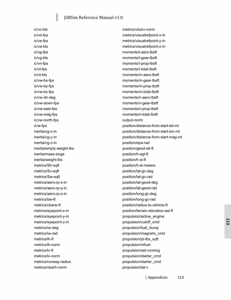
JSBSim Reference Manual v1.0
| Appendices 113
113
ic/vc-kts ic/vd-fps ic/ve-fps ic/ve-kts ic/vg-fps ic/vg-kts ic/vn-fps ic/vt-fps ic/vt-kts ic/vw-bx-fps ic/vw-by-fps ic/vw-bz-fps ic/vw-dir-deg ic/vw-down-fps ic/vw-east-fps ic/vw-mag-fps ic/vw-north-fps ic/w-fps inertia/cg-x-in inertia/cg-y-in inertia/cg-z-in inertia/empty-weight-lbs inertia/mass-slugs inertia/weight-lbs metrics/Sh-sqft metrics/Sv-sqft metrics/Sw-sqft metrics/aero-rp-x-in metrics/aero-rp-y-in metrics/aero-rp-z-in metrics/bw-ft metrics/cbarw-ft metrics/eyepoint-x-in metrics/eyepoint-y-in metrics/eyepoint-z-in metrics/iw-deg metrics/iw-rad metrics/lh-ft metrics/lh-norm metrics/lv-ft metrics/lv-norm metrics/runway-radius metrics/vbarh-norm
metrics/vbarv-norm metrics/visualrefpoint-x-in metrics/visualrefpoint-y-in metrics/visualrefpoint-z-in moments/l-aero-lbsft moments/l-gear-lbsft moments/l-prop-lbsft moments/l-total-lbsft moments/m-aero-lbsft moments/m-gear-lbsft moments/m-prop-lbsft moments/m-total-lbsft moments/n-aero-lbsft moments/n-gear-lbsft moments/n-prop-lbsft moments/n-total-lbsft output-norm position/distance-from-start-lat-mt position/distance-from-start-lon-mt position/distance-from-start-mag-mt position/epa-rad position/geod-alt-ft position/h-agl-ft position/h-sl-ft position/h-sl-meters position/lat-gc-deg position/lat-gc-rad position/lat-geod-deg position/lat-geod-rad position/long-gc-deg position/long-gc-rad position/radius-to-vehicle-ft position/terrain-elevation-asl-ft propulsion/active_engine propulsion/cutoff_cmd propulsion/fuel_dump propulsion/magneto_cmd propulsion/pt-lbs_sqft propulsion/refuel propulsion/set-running propulsion/starter_cmd propulsion/starter_cmd propulsion/tat-c
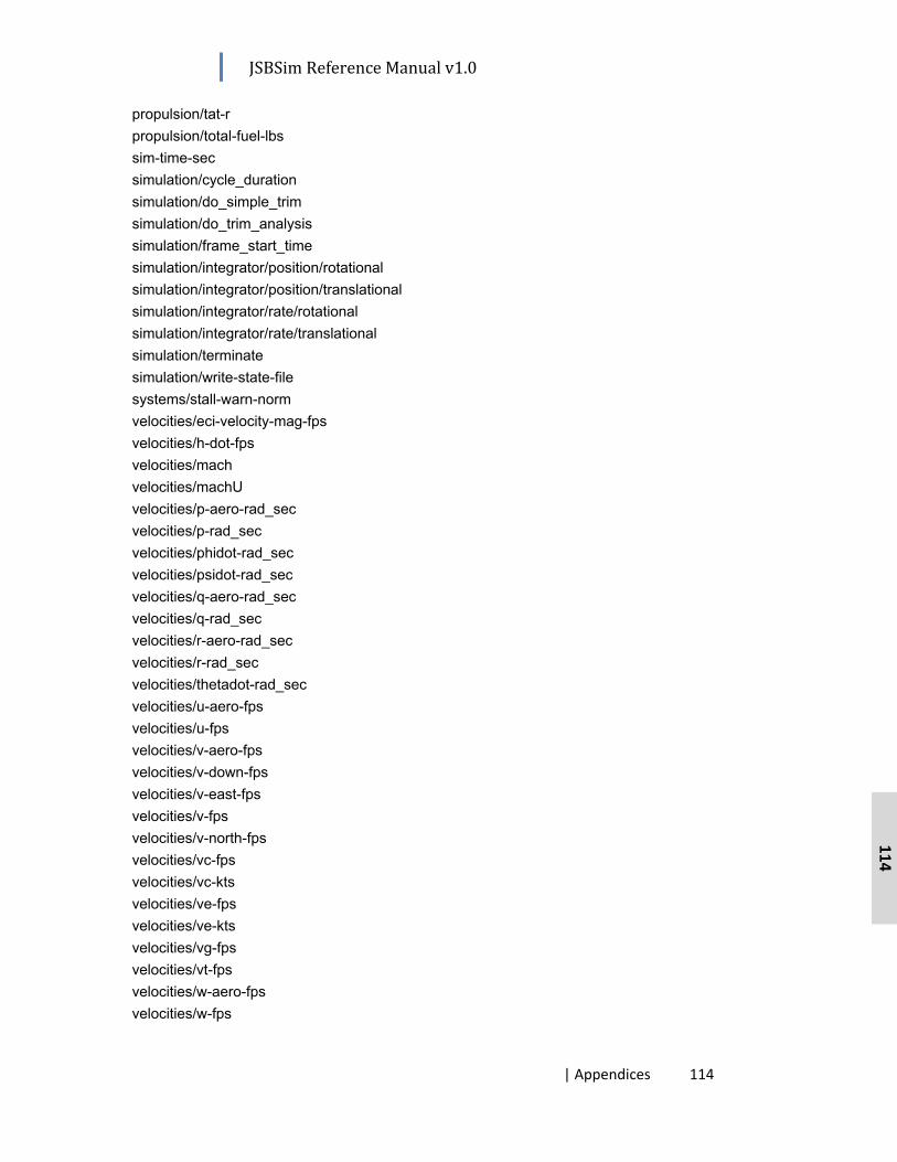
JSBSim Reference Manual v1.0
| Appendices 114
114
propulsion/tat-r propulsion/total-fuel-lbs sim-time-sec simulation/cycle_duration simulation/do_simple_trim simulation/do_trim_analysis simulation/frame_start_time simulation/integrator/position/rotational simulation/integrator/position/translational simulation/integrator/rate/rotational simulation/integrator/rate/translational simulation/terminate simulation/write-state-file systems/stall-warn-norm velocities/eci-velocity-mag-fps velocities/h-dot-fps velocities/mach velocities/machU velocities/p-aero-rad_sec velocities/p-rad_sec velocities/phidot-rad_sec velocities/psidot-rad_sec velocities/q-aero-rad_sec velocities/q-rad_sec velocities/r-aero-rad_sec velocities/r-rad_sec velocities/thetadot-rad_sec velocities/u-aero-fps velocities/u-fps velocities/v-aero-fps velocities/v-down-fps velocities/v-east-fps velocities/v-fps velocities/v-north-fps velocities/vc-fps velocities/vc-kts velocities/ve-fps velocities/ve-kts velocities/vg-fps velocities/vt-fps velocities/w-aero-fps velocities/w-fps

JSBSim Reference Manual v1.0
| Appendices 115
INDEX
< <actuator> .............................. 43 <aero_centered> .................... 39 <aerodynamics> ..................... 14 <aerosurface_scale> ...... 8, 38, 39 <author>................................. 79 <autopilot> ........................ 21, 22 <axis> ............................... 14, 15 <bias> ......................... 38, 43, 44 <bits> ..................................... 44 <c1> ............................ 34, 35, 36 <c2> ....................................... 35 <c3> ....................................... 35 <c4> ....................................... 35 <channel> ...........................8, 21 <clipto> ...............................8, 34 <condition> ............................ 49 <deadband_width> ................ 43 <deadband> ........................... 40 <default> ........................... 21, 37 <description> .............. 10, 11, 49 <domain> ............................... 39 <drift_rate> ............................ 44 <event> .................................. 49 <fcs_function> ....................... 42 <filecreationdate> .................. 79 <fileheader> ........................... 79 <flight_control> ..................8, 21 <function> 10, 11, 14, 15, 19, 42 <gain> ..................... 9, 21, 39, 40 <hysteresis_width> ................ 43 <independentVar> 10, 11, 15, 19,
40, 42 <input> ...............................8, 21 <integrator> ........................... 36 <kd> ....................................... 21 <ki>........................................ 21 <kinematic> ........................... 41 <kp> ....................................... 21 <lag_filter> ....................... 34, 35 <lag> ................................. 43, 44 <lead_lag_filter> .................... 35 <max> ............................... 34, 44 <metrics> ............................... 79 <min> ............................... 34, 44 <noise_variation> .................. 44 <notify> ................................. 49 <pid> ...................................... 21 <position> .............................. 41 <product> ........ 10, 11, 15, 19, 42 <property> ...... 10, 11, 15, 19, 49 <pure_gain> .................. 8, 21, 38 <quantization> ....................... 44 <range> ...............................8, 39 <rate_limit> ........................... 43 <run> ..................................... 49 <runscript> ............................. 49
<scheduled_gain> ............. 39, 40 <second_order_filter> ............ 36 <sensor> ................................. 44 <set> ......................................... 49 <setting> ................................. 41 <sum> ..................................... 10 <summer> .......................... 8, 38 <switch> ........................... 21, 37 <system> ................................ 21 <table>10, 11, 14, 15, 19, 39, 40,
42 <tableData> ... 10, 11, 15, 19, 39,
40, 42 <test> ................................ 21, 37 <time> .................................... 41 <traverse> ............................... 41 <trigger> ................................. 36 <use> ...................................... 49 <value> ................................... 10 <version> ................................ 79 <washout_filter> .................... 35 <width> .................................. 40 <wingspan> .............................. 5
A Aerodynamic coefficients ....... 13 Aerodynamics ......................... 13 Autopilot
Wing leveler ...................... 87 axis elements .......................... 14
B Body frame .......... See Frames of
reference Building JSBSim ...................... 1
C Class heirarchy ....................... 56 Coefficient buildup method .... 16 CVS .......................................... 1
D Downloading ............................ 1
E ECEF (Earth-Centered, Earth-
Fixed) ............. See Frames of reference
ECI (Earth-Centered, Inertial) ....... See Frames of reference
English Units ............... See Units Equations of Motion ............... 69
F Flight control components
Absolute value .................. 41 Actuator ............................ 42 Aerosurface scaling .......... 38 Deadband .......................... 40 Filters ................................ 34 Function ............................ 42 Gain .................................. 38 Hysteresis ......................... 41 Integrator .......................... 36 Kinematic ......................... 41 Lag filter ........................... 34 Lead-lag filter ................... 35 Limiter .............................. 41 Positive or negative value . 41 Sample and hold ............... 37 Scheduled gain .................. 39 Second order filter ............ 35 Sensor ............................... 43 Summer ............................. 38 Switch ............................... 36 Washout filter ................... 35
Frames of reference Body frame ......................... 5 Body-fixed ........................ 69 ECEF ................................ 69 ECI .................................... 70 NED .................................. 69 Stability frame .................... 5 Structural frame .................. 4 Wind frame ......................... 5
Functions .................................. 9
M Math
Tables ............................... 11 Metric Units ................ See Units
N NED (North-East-Down) ...... See
Frames of reference
P PID controller............. 25, 44, 88
tuning ................................ 89 Properties ................................. 7
R Reference frames . See Frames of
reference Running JSBSim ...................... 1

JSBSim Reference Manual v1.0
| Appendices 116
S Scripts .................................... 49 Stability frame ..... See Frames of
reference Structural frame ... See Frames of
reference System components ............... 21
T Tables .......................... See Math TCDS (Type Certificate Data
Sheet) ................................ 16
U Units ......................................... 5
W Wind frame .......... See Frames of
reference Wing leveler .......... See Autopilot