Julio González-Díaz, Ignacio Palacios-Huerta

Cognitive performance in competitive environments: evidence from a natural experiment Article (Accepted version) (Refereed)

Original citation: González-Díaz, Julio and Palacios-Huerta, Ignacio (2016) Cognitive performance in competitive environments: evidence from a natural experiment. Journal of Public Economic, 139. pp. 40-52. ISSN 0047-2727 DOI: 10.1016/j.jpubeco.2016.05.001 Reuse of this item is permitted through licensing under the Creative Commons:

© 2016 Elsevier B.V. CC BY-NC-ND 4.0 This version available at: http://eprints.lse.ac.uk/67144/ Available in LSE Research Online: July 2016

LSE has developed LSE Research Online so that users may access research output of the School. Copyright © and Moral Rights for the papers on this site are retained by the individual authors and/or other copyright owners. You may freely distribute the URL (http://eprints.lse.ac.uk) of the LSE Research Online website.

�������� ����� ��

Cognitive Performance in Competitive Environments: Evidence from aNaturalExperiment

Julio Gonzalez-Dıaz, Ignacio Palacios-Huerta

PII: S0047-2727(16)30046-9DOI: doi: 10.1016/j.jpubeco.2016.05.001Reference: PUBEC 3669

To appear in: Journal of Public Economics

Received date: 2 October 2014Revised date: 4 May 2016Accepted date: 5 May 2016

Please cite this article as: Gonzalez-Dıaz, Julio, Palacios-Huerta, Ignacio, CognitivePerformance in Competitive Environments: Evidence from aNatural Experiment, Journalof Public Economics (2016), doi: 10.1016/j.jpubeco.2016.05.001

This is a PDF file of an unedited manuscript that has been accepted for publication.As a service to our customers we are providing this early version of the manuscript.The manuscript will undergo copyediting, typesetting, and review of the resulting proofbefore it is published in its final form. Please note that during the production processerrors may be discovered which could affect the content, and all legal disclaimers thatapply to the journal pertain.

ACC

EPTE

D M

ANU

SCR

IPT

ACCEPTED MANUSCRIPT

Cognitive Performance in Competitive Environments:Evidence from a Natural Experiment∗

Julio Gonzalez-Dıaz† Ignacio Palacios-Huerta‡

May 2016

AbstractCompetitive situations that involve cognitive performance are widespread in

labor markets, schools, and organizations, including test taking, competition forpromotion in firms, and others. This paper studies cognitive performance in ahigh-stakes competitive environment. The analysis takes advantage of a naturalexperiment that randomly allocates different emotional states across professionalsubjects competing in a cognitive task. The setting is a chess match where twoplayers play an even number of chess games against each other alternating the colorof the pieces. White pieces confer an advantage for winning a chess game and whostarts the match with these pieces is randomly decided. The theoretical analysisshows that in this setting there is no rational reason why winning frequenciesshould be better than 50-50 in favor of the player drawing the white pieces in thefirst game. Yet, we find that observed frequencies are about 60-40. Differences inperformance are also stronger when the competing subjects are more similar incognitive skills. We conclude that the evidence is consistent with the hypothesisthat psychological elements affect cognitive performance in the face of experience,competition, and high stakes.

∗We thank Luis Cabral, David De Meza, Leontxo Garcıa, Diego Gonzalez-Dıaz, Robert Ostling,Pedro Rey-Biel, Yona Rubinstein, David Stromberg, Richard Thaler, Oscar Volij, two anonymousreferees, and participants in seminars at LSE, Bristol, Munich, Pisa, Stockholm IIES, Erasmus, BenGurion, Collegio Carlo Alberto, IMEBE and the Chess Grand Slam Final Bilbao-Shanghai for use-ful comments. Financial support from the Spanish Ministerio de Economıa y Competitividad andFEDER (projects MTM2011-27731-C03, MTM2014-60191-JIN, ECO2012-31626, ECO2015-66027-P),from Xunta de Galicia (project INCITE09-207-064-PR), and from the Departamento de Educacion,Polıtica Linguıstica y Cultura del Gobierno Vasco (IT-869-13) is gratefully acknowledged.

†Universidad de Santiago de Compostela. Email: julio.gonzalez@usc.es‡London School of Economics and Ikerbasque Foundation at UPV/EHU. Email: i.palacioshuerta@

gmail.com

1

ACC

EPTE

D M

ANU

SCR

IPT

ACCEPTED MANUSCRIPT

1 Introduction

In recent years, economists have paid considerable attention to the relationship betweenperceptions and reasoning, and to emotions such as loss aversion, reference points,disappointment and others. There is evidence that these and other behavioral effectsare in fact important for explaining a wide range of economic and social behavior. 1

Despite their potential importance, however, little is known about the relevance ofthese effects on cognitive performance. Do they exist? If so, do they persist in the faceof experience, competition, and high stakes? These are the questions we study in thispaper.

Understanding cognition is important. Numerous studies establish that measuredcognitive ability is a strong predictor of occupational attainment, wages, and a rangeof social behaviors in adults, and several studies document its importance in predictingthe schooling performance of children and adolescents.2 An emerging body of literaturealso finds that “psychic” costs explain a range of economic and social behavior (see,e.g., Carneiro, Hansen, and Heckman (2003), Carneiro and Heckman (2003), Cunha,Heckman and Navarro (2005), Heckman, Lochner and Todd (2006)). Besides social andeconomic outcomes, recent research shows that cognitive ability is also important forfinancial market outcomes.3 Thus, numerous settings represent competitive situationsthat involve cognitive performance (e.g., test taking, student competition in schools,competitions for promotion in certain firms and organizations, and others), and under-standing the relationship between cognitive performance and psychological effects is animportant question in the literature on human capital, schooling, behavioral economicsand others.

This paper contributes to these strands of economics literature by studying the im-pact of psychological differences on cognitive performance in a competitive environment.The analysis benefits from the opportunity provided by a randomized natural exper-iment that, in effect, exogenously assigns different emotional states across subjects.Similar natural experiments to the one we study have been used to examine the role ofpsychological effects when subjects perform non-cognitive tasks, and this paper extends

1Rabin (1998), Camerer (2003) and DellaVigna (2009) provide excellent surveys.2See, for instance, Neal and Johnson (1996), McArdle, Smith and Willis (2009), and other references

therein. Heckman, Stixrud and Urzua (2006) review this literature and present an analysis of the effectsof both cognitive and noncognitive skills on wages. They show that a model with one latent cognitiveskill and one latent noncognitive skill explains a large array of diverse behaviors including schooling,work experience, occupational choice, and participation in various adolescent risky behaviors.

3See, for instance, Agarwal and Mazumder (2013), Bertrand and Morse (2011), Gerardi, Goette andMeier (2010), and Cole and Shastry (2009).

2

ACC

EPTE

D M

ANU

SCR

IPT

ACCEPTED MANUSCRIPT

the analysis to study their impact on the performance in cognitive tasks. As such, andto the best of our knowledge, it represents the first study that evaluates the causallink from behavioral effects to cognitive performance in a competitive setting takingadvantage of a natural experiment.

The randomized experiment comes from professional sports. Important elementsof human behavior are starkly observable in these settings. As Rosen and Sanderson(2001) indicate, “if one of the attractions of sports is to see occasionally universal as-pects of the human struggle in stark and dramatic forms, their attraction to economistsis to illustrate universal economic principles in interesting and tractable ways.” Thus,not surprisingly, a number of prominent findings in economics have been documentedfor the first time studying sports settings. For instance, without attempting to beexhaustive, Ehrenberg and Bognano (1990) investigate incentive effects in golf tourna-ments, Szymanski (2000) studies discrimination using soccer data, Garicano et al (2006)study social pressure as a determinant of corruption in a soccer setting, and Bhaskar(2009) and Romer (2006) analyze optimal decision-making using cricket and footballdata respectively.

Much like these sports settings, ours represents a valuable opportunity for studyingan open question in the literature for a number of reasons:

First, the situation involves a tractable number of subjects (just two) competing ata game that is considered the ultimate cognitive sport (chess). The game they play hascomplete information and involves no chance elements. The game is strictly competitiveor zero-sum. Pure conflict situations in which one person’s gain is always identical toanother’s loss involve no potential elements of cooperation. As such they represent thecleanest possible context to study competitive behavior. Subjects compete in the samesetting and under identical circumstances and, as we will see in the next section, theonly difference is the randomly determined order in which they complete a task.

Second, and most importantly, we take advantage of existing results in the literature(to be discussed below) that show that the order of competition generates differencesin emotional states. Using the same type of randomly assigned treatment and controlof these emotional states we extend existing research to the study of performance oncognitive tasks in a competitive environment.4

Third, the setting involves professional subjects who are characterized by the highestdegree of cognitive skills at the specific competitive task they perform as professionals

4As is well known, a randomized experiment is a powerful methodology not often available in thesocial sciences that ensures that the conditions for causal inference are satisfied (Manski, 1995). Thereis also a related literature suggesting that providing relative performance information (a consequenceof the order of competition in our setting) affects performance (Azmat and Iriberri, 2010).

3

ACC

EPTE

D M

ANU

SCR

IPT

ACCEPTED MANUSCRIPT

(playing chess). Thus, we can study if biases exist in the face of experience, competi-tion and high stakes. This is also important because existing research has found thatindividuals with higher cognitive ability demonstrate fewer and less extreme cognitivebiases that may lead to suboptimal behavior.5

Fourth, direct measures of cognitive abilities are often lacking in the literature andcan be measured only indirectly (through their correlation with other variables). Thesetting in this paper provides a highly precise measure of the cognitive ability of theplayers at the task they perform. In particular, subjects have a rating according towhat is called the “ELO rating method” (see Section 4), and this rating estimates quiteprecisely the probability that one player will outperform the other at the cognitive task.This is a valuable advantage of the empirical setting.

Finally, the study concerns high-stakes decisions that subjects are familiar with,that really affect them, to which they are used, and that take place in their own real-lifeenvironment. In this sense, it involves a set of useful characteristics in terms of stakes,familiarity and nature of the environment. And from the perspective of observing andmeasuring behavior, a comprehensive dataset is available where choices, outcomes, andtreatments are cleanly measured.

From the theoretical point of view, we also develop rational and behavioral models ofoptimal play to interpret the empirical evidence. Importantly, these models will containa contribution to the game theoretical literature on repeated interactions and to theliterature on multi-battle contests. In our setting, a match consists in the repeated playof a given stage game but, differently from standard repeated games, the total payoffthat players obtain may not be a sum or an average of the payoffs in each period. Theexisting literature has studied the case of binary outcomes: in each stage game oneplayer wins and the other loses (see Walker, Wooders and Amir (2011)), but we areaware of no study with more than two outcomes. The presence of a third outcome (inour context, win, lose, and tie) brings in the issue of how to chose risk during the match,which we incorporate into the formal frameworks. This represents a novel aspect withrespect to the literature on multi-battle contests in which strategic risk taking is not achoice variable (e.g., Konrad and Kovenock (2009)).

The rest of the paper is structured as follows. Section 2 describes the natural exper-iment and a brief literature review. Section 3 develops formal rational and behavioralmodels of the task the subjects undertake. The models allow us to identify the condi-tions under which we may be able to conclude, using the average treatment effects from

5See, for instance, the recent results in Gill and Prowse (2015). Also, Benjamin, Brown and Shapiro(2013) and Frederick (2005) report similar findings for high school and college students, respectively,using different measures of intelligence and cognitive ability.

4

ACC

EPTE

D M

ANU

SCR

IPT

ACCEPTED MANUSCRIPT

the natural experiment, whether behavioral elements have an impact on cognitive per-formance. Section 4 describes the data. Section 5 presents the main empirical evidence,and Section 6 concludes.

2 The Natural Experiment

In a chess match, two players play an even number of chess games, typically about 6 to10 games, against each other. Games are generally played one per day, with one or tworest days during the duration of the match. The basic procedure establishes that thetwo players alternate the colors of the pieces with which they play. In the first game,one player plays with the white pieces and the other with the black pieces. In the secondgame, the colors are reversed, and so on. Who plays with the white pieces in the firstgame is randomly determined, and this is the only procedural difference between thetwo players. According to the rules of FIDE (the Federation Internationale d’ Echecs,the world governing body of chess), the order is decided randomly under the supervisionof a referee. This random draw of colors, which is typically conducted publicly duringthe opening ceremony of the match, requires that the player who wins the draw willplay the first game with the white pieces. Therefore, the fact that players have no choiceof order or color of the pieces makes it an ideal randomized experiment for empiricallyestablishing causality.

The explicit randomization mechanism used to determine which player begins withthe white pieces in a sequence of games where both players have exactly the sameopportunities to play the same number of games with the same colors, have the samestakes, are in the same setting and where all other circumstances are identical, suggeststhat we should expect both players to have, ceteris paribus, exactly the same probabilityof winning the match. That is, absent behavioral effects associated with the order ofcolors, there is no rational reason why observed winning frequencies should be differentfrom 50-50.6 Yet, we find that this is not the case. As anticipation of the results, whatwe observe instead is that winning probabilities are about 60-40 in favor of the playerwho plays with the white pieces in the first and in all the odd games of the match.

As will be discussed in more detail later, playing with the white pieces is advanta-geous to win a chess game. This means that, ceteris paribus, the player playing with thewhite pieces in the odd games of the match is randomly allocated a greater likelihoodto be leading during the course of the match. Conversely, his opponent, who plays withthe white pieces in the even games of the match, is more likely to be lagging. Hence,this natural experiment shares the same basic design used recently in the literature to

6In Section 3 we qualify this statement.

5

ACC

EPTE

D M

ANU

SCR

IPT

ACCEPTED MANUSCRIPT

study the relevance of emotional or psychological states in understanding the behaviorof subjects performing non-cognitive tasks in competitive environments. In particular,Genakos and Pagliero (2012), Pope and Schweitzer (2011), Apesteguia and Palacios-Huerta (2010), and Genakos, Pagliero, and Garbi (2015) provide strong evidence forthese effects from weightlifting, golf, penalty kicks in soccer, and diving competitions,respectively. Our study, therefore, extends exisiting research to the area of cognitiveperformance in a competitive environment using the same type of randomly determinedasymmetry in emotional states. With respect to the term “emotional states,” Sokol-Hessner et al (2009) document how loss aversion is a basic hedonic property of ourreaction to losing. In particular, they combine physiological measurements of arousaland various cognitive strategies to study how differences in arousal to losses relative togains correlates with behavioral loss aversion. It is in this sense that we refer throughoutthe paper to the random determination of the order of play (the advantage of playingwith the white pieces in the even games) as effectively randomizing emotional states.7

Finally, it seems appropriate to quote a reflection by Osborne and Rubinstein (1994,p.6) who were the first to identify the research potential of this specific natural set-ting (chess) to contribute to our understanding of bounded rationality, including therelationship between cognitive abilities and behavioral effects (italics added):

“When we talk in real life about games we often focus on the asymmetry betweenindividuals in their abilities. For example, some players may have a clearer perceptionof a situation or have a greater ability to analyze it. These differences, which are socritical in real life, are missing from game theory in its current form. To illustrate theconsequences of this fact, consider the game of chess. In an actual play of chess theplayers may differ in their knowledge of the legal moves and in their analytical abilities.In contrast, when chess is modeled using current game theory it is assumed that theplayers’ knowledge of the rules is perfect and their ability to analyze it ideal. Resultswe prove [...] imply that chess is a trivial game for “rational” players: an algorithmexists that can be used to “solve” the game. This algorithm defines a pair of strategies,one for each player, that leads to an “equilibrium” outcome with the property that aplayer who follows this strategy can be sure that the outcome will be at least as good asthe equilibrium outcome no matter what strategy the other player uses. The existenceof such strategies (first proven by Zermelo (1913)) suggests that chess is uninterestingbecause it has only one possible outcome. Nevertheless, chess remains a very popularand interesting game. Its equilibrium outcome is yet to be calculated; currently it isimpossible to do so using the algorithm. Even if White, for example, is shown one day

7Other references with neurological and physiological evidence that support our use of these termsinclude Bechara et al. (1997), Schaefer et al. (2002), Ochsner et al. (2004), and Kerner et al. (2006).

6

ACC

EPTE

D M

ANU

SCR

IPT

ACCEPTED MANUSCRIPT

to have a winning strategy, it may not be possible for a human being to implementthat strategy. Thus, while the abstract model of chess allows us to deduce a significantfact about the game, at the same time it omits the most important determinant of theoutcome of an actual play of chess: the players’ “abilities.” Modeling asymmetries inabilities and in perceptions of a situation by different players is a fascinating challengefor future research, which models of “bounded rationality” have begun to tackle.”

To the best of our knowledge, no previous research has taken the opportunity thatthis setting provides to study these aspects.

3 Rational and Behavioral Models of a Match

A chess match is a nontrivial setting in which it is not possible to attribute differencesin performance, if any, without first understanding what is the role that rational andbehavioral elements may play in behavior. So, what is the role that these elementsplay in a chess match? Under what conditions may we conclude that psychological orrational effects have an impact on cognitive performance? In this section we provide aformal analysis to address these questions.

Recall that the randomly determined color of pieces generates one very specific typeof asymmetry between the players: as playing with white pieces confers a strategicadvantage in a chess game,8 the random draw of colors means that players who beginplaying with the white pieces are randomly given a greater opportunity to lead in thematch and, conversely, those with the black pieces are given a greater opportunity tolag in the match.

We start with a canonical model (Subsection 3.1), which we then develop to includerational and psychological elements (Subsections 3.2 and 3.3). For the sake of exposition,we use chess terminology. Needless to say, the analysis also applies to other settingswith repeated interactions in which the stage games have three possible outcomes.

3.1 The Canonical Model

Consider a chess game between two identical players: white and black. Let W > 0denote the probability that the player with the white pieces (white) wins and L > 0

8In the sample of matches we will study, 30 percent of the games were won by the players with thewhite pieces and 17 percent by the player with the black pieces; the rest are draws. In the more than165,000 chess games in the Chessbase dataset presented in the next section, which includes our datafrom chess matches, the win rates are 28 and 18 percent, respectively, when both players have an ELOrating above 2,500 (typically Grandmasters, the highest title a player can achieve).

7

ACC

EPTE

D M

ANU

SCR

IPT

ACCEPTED MANUSCRIPT

the probability that the player with the black pieces (black) wins. We assume thatW + L < 1, so 1−W −L > 0 is the probability that the game ends in a draw. In chessit is strategically advantageous to play with the white pieces, which means that W > L.As just noted, empirically W is about 0.28-0.30 and L about 0.17-0.18.

A canonical chess match consists of T chess games, where T is an even number.In game 1, Player 1 plays with the white pieces and Player 2 with the black ones. Insubsequent games the colors are alternated. Since a chess match is a constant-sumgame, then, without loss of generality, we can assume that the utilities for each of theplayers are 1 if winning the match, 0 if losing, and 0.5 if they tie.9

Since both players are completely symmetric in a canonical chess match, the followingresult is straightforward:

Proposition 3.1. The expected payoff in a canonical chess match is 0.5 for both players.

3.2 Rational Models

Preliminaries. A chess match is a dynamic tournament in which, in principle, play-ers may not have the same effort conditions during the match and/or may choose theamount of risk to take depending on their leading/lagging state in the score. Typi-cally, in the empirical studies in the literature that study non-cognitive performancein competitions, the task is effortless and risk either does not play any role (when theoutcome of the task is binary, e.g., score or not) or can be cleanly taken into account. 10

In a chess game, however, strategic risk taking matters since there are three possibleoutcomes (either player may win the game or they may tie).

In what follows we try to understand the role that effort and risk may play in ourempirical setting:

a. Effort. With respect to the idea that players can exert different effort duringthe match depending on the score, the design by FIDE of the typical chess matchintends to ensure that all the games in the match are played under identical conditionsand, in particular, that players have sufficient time to fully recover from the effortthey exert: no more than one game is played each day and rest days are scatteredduring the duration of the match to ensure that players can play every single game inperfect physical conditions and can always exert the maximum cognitive effort. This

9Since both players are identical, we can represent their preferences by the same utility functions.Then, without loss of generality, these utilities can be normalized so that the utility of a win is 1 andthe utility of a loss is 0. Hence, since we are in a constant-sum game, the utility of a tie has to be 0 .5.

10See, for example, Genakos and Pagliero (2012) and Apesteguia and Palacios-Huerta (2010).

8

ACC

EPTE

D M

ANU

SCR

IPT

ACCEPTED MANUSCRIPT

characteristic allows us to abstract from modelling effort as a choice variable. 11

b. Risk. A more important consideration is the fact that players may choose therisk they take during the match depending on the score. The role of strategic risktaking is, in general, not trivial and requires a formal analysis, which we provide below.Interestingly, the analysis shows that strategic risk taking is not neutral: it favors theplayer who starts the match playing with the black pieces. That is, absent behavioraleffects this player should win significantly more often a chess match. The basic intuitionfor this result is the following. Lagging in the score may induce a player to choose tolower his expected performance by taking risks that he would otherwise not take inexchange for a greater probability to win a game and catch up in the score. Hence,the possibility of taking more risks and having more variable outcomes (e.g., increasingthe chance of both winning and losing in exchange for a lower chance of tying) is aninstrument at the disposal of the lagging player. This instrument, if anything, couldhelp counteract any potential disadvantages given by the random determination of thecolors. Clearly, the leading player can also tailor the risk he takes to the advantage thathe has in the match and play more conservative strategies. However, no matter howconservative the leading player is, the lagging player can always drive the game into awin-lose lottery where the probability of winning is greater than if he had not chosento take the additional risk.

This insight is not new; in fact, it is well known in the literature on the strategicchoice of risk (variance and covariance) in dynamic competitive situations. 12 Yet, asindicated earlier, it has been studied neither in the game theoretical literature on re-peated interactions nor in the literature on multi-battle contests. In terms of empiricalimplications, it means that if the player who starts the match playing with the blackpieces exhibits significantly greater cognitive performance, then empirical evidence fromaverage treatment effects alone will not allow us to conclude whether behavioral effectsare present in the data. The reason being that his greater winning frequency may simply

11In related settings studied in the literature, effort is a choice variable. There is a body of literaturethat studies multi-battle contests in which players compete in a sequence of single component contests(battles) choosing effort (e.g., monetary expenditures). Importantly, in these settings, and differentfrom ours, effort determines the size of the prize both in the component battles and in the overallbattle. See for example Harris and Vickers (1987) in the context of a patent race, and Klumpp andPolborn’s (2006) study of the dynamics of candidate performance and campaign expenditures in theUS presidential primaries. Konrad and Kovenock (2009) characterize the unique subgame perfectequilibrium in these multi-battle contests when effort is a choice variable, but strategic risk taking isabsent. Interestingly, in their setting, having effort as a choice variable is neutral in that it does notcause any deviation from 50-50 in the probability of winning the contest. For a survey of the theory ofcontests in sports see Szymanski (2003).

12See, for instance, Cabral (2002, 2003), Hvide (2002) and Hvide and Krinstiansen (2003).

9

ACC

EPTE

D M

ANU

SCR

IPT

ACCEPTED MANUSCRIPT

reflect the advantage that strategic risk taking confers.Before formalizing the role of strategic risk taking we discuss an assumption specific

to the empirical setting.

Assumption. In a typical chess game, the first mover advantage gives the playerwith the white pieces at least as much control over how “risky” the game will be. This isbecause he has at least as much control over the type of “opening” that will be played.Although there is not much discussion about this assumption in the chess community,chess is too complex to provide a theoretical foundation for it. We incorporate thisasymmetry in the “technology” for risk taking in the models and provide two pieces ofsupport for this assumption:

1. Experts’ Assessment. It is not difficult to find statements from world elite playersthat support this assumption. For instance, former world champion Vladimir Kramnik(June 2011, interviewed after the Candidates Matches to qualify to challenge the reigningworld champion, italics added) indicates: “My white games were all pretty complicated,tense and full of fight. I am responsible for my white games, and I was always trying tofind a way to fight with white, even if I did not get an advantage. But with black it isvery difficult and incredibly risky to start avoiding drawish lines from the very beginning,because it can easily just cost you a point in a very stupid way [...] get a bad position,lose the game, lose the match and feel like an idiot? I didn’t do it [...]. It is a difficultdecision which can easily backfire at this level.”

2. Empirical Evidence. We know that because of strategic risk taking the expectedperformance of a player in a game should decrease when he is lagging. As a result, theassumption on the asymmetric technology for risk taking has the additional implicationthat it should decrease by a greater amount when the black player is lagging than whenthe white player is lagging. The empirical evidence is consistent with this implication:when lagging the observed decrease in performance is more than twice as large for black(about 16 percent) than for white (about 7 percent).13

13The expected performance is simply the number of points a player is expected to achieve inthe current game. That is, his expected score can be computed as 1 × “prob. of winning” + 0.5 דprob. of a draw” + 0 × “prob. of losing”. The table below shows the expected score for each playerwhen lagging and when the match is tied for matches between players with ratings above 2500 (typicallyGrandmasters). Similar results are found for all other subsets we have examined, and for the wholesample of matches. Performance loss denotes the relative change in the expected score.

ELO ratings above 2500Expected score of white Expected score of black

Match tied 0.553 Match tied 0.447White lagging 0.515 Black lagging 0.374

Performance loss 6.9% Performance loss 16.3%

10

ACC

EPTE

D M

ANU

SCR

IPT

ACCEPTED MANUSCRIPT

Models. We now present two models which incorporate into the canonical modelthe assumption that the “technology” for risk-return trade-off is at least as good for theplayer with the white pieces than for his opponent. Importantly, we will find that thisassumption is sufficient (but not necessary) to show that the possibility of choosing therisk that is taken favors the player starting with the black pieces. The reason is that themain element driving the result is not this assumption but the “informational rent” ofthe player starting with the black pieces: Since risk taking increases the probability ofwinning a game at the cost of increasing by a larger amount the probability of losing, risktaking is especially useful for a lagging player. The intuition is again straightforward.Take a two-game match and suppose that the player starting with black has lost thefirst game. Then, in the second game, a draw is as bad as a loss and therefore he onlycares about increasing his probability of winning. He will surely take risks regardless ofwhether or not white has more control over risk. Of course, the same would be true forthe player starting with the white pieces if he had lost the first game, but this effectis less important since the probability of winning with the white pieces is greater thanwith the black pieces.

Model R1: Only White Controls Risk

In this first model we assume that white has all the control over the risk involved inthe game, an assumption that we relax in the following model by assuming that blackalso has some control over the risk. By taking a risky action, white can increase hisprobability of winning by Rw > 0 and his probability of losing by αRw, with α > 1.14

Recall that in game 1 Player 1 plays with the white pieces and Player 2 with the blackones. Since white has all control over risk, Player 2 can guarantee for himself an expectedpayoff of at least 0.5 by mimicking in the even games the choices made by Player 1 inthe odd games. We show below that Player 2 can in fact do strictly better. Intuitively,this is because he can benefit from the fact that he has more information when he hasto make his choices concerning optimal risk-taking.

Proposition 3.2. Consider a match consisting of T = 2 games in Model R1. Then,optimal play in this match leads to a higher expected payoff for Player 2 than for Player 1.

Proof: See Appendix A.

Corollary 1. In a match consisting of T games in Model R1, the expected payoff forPlayer 2 is greater than the expected payoff for Player 1.

14Of course, we assume that W + L + (1 + α)Rw < 1.

11

ACC

EPTE

D M

ANU

SCR

IPT

ACCEPTED MANUSCRIPT

Proof: See Appendix A.

The proofs of these results show that the empirical fact that W > L is not necessary.Since Player 2 is the only one who can choose risk in Period 2, he is also the first onewho can make an informed choice of risk. This “informational rent” is enough to givehim an edge in the match.

We show in the next model that if both players have some control over risk in bothperiods, then the fact that W > L is crucial to prove that Player 2 has an advantage.

Model R2: Both Players Control Risk

In a given game both players can increase the probability of winning by taking arisky action. A risky action by white increases his probability of winning by Rw > 0and his probability of losing by αRw, with α > 1. Similarly, a risky action by blackincreases his probability of winning by Rb ≥ 0 and his probability of losing by αRb.

15

Under the assumption that white has at least as much control over how “risky” a chessgame is, we have Rw ≥ Rb. We find below that this is a sufficient condition to obtainthat Player 2 has an advantage in a match. Further, this condition is not necessary.

Note that, since W > L and α > 1, the following two conditions are satisfied whenRw ≥ Rb:

C1: Rb < WL

Rw.

C2: Rb < Rw + Rw(α−1)(1−W−Rb)L+Rw

.

We show next that these two conditions suffice to give Player 2 an advantage in atwo-game match. The intuition is that, although both players can control risk in bothperiods, the possibility of choosing a risky strategy is particularly valuable when a playeris lagging in the score. Since W > L, Player 2 is more likely to be lagging in the scorethan Player 1 and, hence, he is the one more likely to benefit from optimal risk takingin Period 2.

Proposition 3.3. Consider a match with T = 2 games in Model R2. When C1 and C2are satisfied, optimal play leads to a higher expected payoff for Player 2. A sufficientcondition for this result is that Rw ≥ Rb.

15Obviously, it has to be the case that W + Rw + αRb + L + Rb + αRw ≤ 1.

12

ACC

EPTE

D M

ANU

SCR

IPT

ACCEPTED MANUSCRIPT

Proof: See Appendix A.

This generalizes Proposition 2.16 Although Rw ≥ Rb is sufficient for this result, itis clear from conditions C1 and C2 that it is not necessary as Player 2 will also havean advantage even in some cases where Rw < Rb. In other words, stating the resultin terms of these two conditions is stronger than stating it in terms of Rw ≥ and Rb.And again the intuition is that the “informational rent” that Player 2 always has isindependent of which player has greater control over risk in a game.

3.3 Behavioral Models

We next extend the canonical and rational models to incorporate psychological elements.We try to adopt the simplest possible formulation that is both tractable and consistentwith empirical evidence. As discussed earlier, empirical evidence from non-cognitivetasks supports the hypothesis that a gain/loss or leading/lagging asymmetry relativeto a reference point has an impact on performance. This is the first aspect that wewant to capture in the model. The literature offers various ways to formalize thisidea. In particular, preferences with loss-aversion relative to a reference point havebeen widely adopted in both theoretical and empirical research, rationalizing a host ofanomalies from labor supply, to consumer behavior and finance. The incorporation ofthese ingredients into economic theory dates back at least to Kahneman and Tversky(1979), and much of the early literature equated the reference point with an exogenousor history-dependent status quo. Recently, Koszegi and Rabin (2006, 2007) suggestedan alternative approach of forward-looking, endogenous reference-point formation basedon expectations. Here we take the simplest possible version and simply assume that twoidentical subjects perceive an even score in the match as their reference point and thattheir performance is a function of whether they are leading or lagging in the score. Aswill be clear below, other formulations are definitely possible. Yet, this one is tractable,proves convenient from a formal perspective, and captures the basic insights of moregeneral formulations.17

16Obviously, when Rb = 0, conditions C1 and C2 are trivially satisfied and this result reduces toProposition 3.2 in Model R1.

17Current research in economic theory is trying to understand how to empirically distinguish amongdifferent models of reference dependence that share similar formulations but specify different processesof reference point formation (see, e.g., see Masatliogu and Raymond (2014)). This is not at all trivial. Infact, providing separation between competing accounts of reference-dependence is empirically difficult,often pushing the limits of experimental feasibility. See Sprenger (2015) for a novel experimentaldesign that successfully accomplish this separation. Distinguishing among competing models, however,is beyond what can be studied in our empirical setting.

13

ACC

EPTE

D M

ANU

SCR

IPT

ACCEPTED MANUSCRIPT

Let k denote the difference between the number of games won and the number ofgames lost by the player who plays with the white pieces; that is, k is positive whenhe is leading and negative when he is lagging. Recall that the natural experimentrandomizes the identity of the players more likely to be leading and lagging in the score.Now, the probability that the player with the white pieces wins the current game isW + e(k) and the probability that he loses is L − e(k), where e(∙) is an increasingfunction that captures the behavioral element with e(0) = 0 . Winning generates elationwhereas losing generates disappointment and discouragement. As we are in a zero-sum game, e(∙) captures this asymmetry and its impact on relative performance. Wefurther assume that − e(−1) ≥ e(1), which means that the decrease in performancewhen lagging by one game for the player with the white pieces is at least as large as theincrease in performance when leading by one game.18 Clearly, e(∙) must also be suchthat W + e(k) ≤ 1, and L − e(k) ≥ 0. This formulation captures in a parsimoniousmanner the basic ingredient of the loss aversion effect typically considered in moregeneral specifications in the literature.19 Players have no control over this effect; inother words it is not under volitional control.20

Model B1: No Strategic Risk Taking

We next prove that when risk taking is not a choice variable Player 1 has an ad-vantage. For intuition note that, since W > L, Player 2 is more likely to start game 2lagging in the score (k = −1) than leading in the score (k = 1), and that the propertiesof e(∙) imply that this effect will negatively affect his performance in game 2.

Proposition 3.4. Consider a match consisting of T = 2 in Model B1. If e(−1) < 0,then the expected payoff of Player 1 is higher than the expected payoff of Player 2.

Proof: See Appendix A.

18“Disappointment,” “elation” and “discouragement” are terms used both in the economics litera-ture (e.g., Gill and Prowse (2012) and Abeler et al (2011) in contexts of effort provision) and in thepsychology literature.

19Golman and Rao (2014) provide supporting evidence for these ingredients from basketball. Usingdata from hundreds of thousands of plays, they find that among NBA players: (1) expectations donot influence the reference point, which appears remarkably stable around zero, and (2) when trailing,players perform worse on focus-intensive effortless tasks (they shoot free throws with lower accuracy),a finding also in Mertel (2011). Also in the context of basketball but at the level of teams, which mayexert effort and choose risk, Berger and Pope (2011) find evidence where lagging by a little at half timecan lead to winning at the end of the match.

20An intriguing theoretical innovation is the possibility of incorporating a conscious choice of antici-pation (how to mentally prepare) as a mechanism through which reference points are formed as beliefs(see Sarver, 2014).

14

ACC

EPTE

D M

ANU

SCR

IPT

ACCEPTED MANUSCRIPT

The proof of this result shows that the edge that the psychological effect gives toPlayer 1 increases with the edge he has in the first game, that is with W − L: Playingthe first game with the white pieces makes his opponent more likely to lag in the matchand thus more likely to be subject to the decrease in performance caused by e(−1). Weshow below that the result extends to matches of arbitrary length.

Proposition 3.5. Consider a match consisting of T games in Model B1. If e(−1) < 0,then the expected payoff for Player 1 is greater than the expected payoff for Player 2.

Proof: See Appendix A.

Model B2: Strategic Risk Taking

Thus far we have seen that strategic risk taking favors Player 2 (Section 3.2) whilepsychological effects e(∙) favor Player 1. Next, we study the model in which both effectsare considered simultaneously and the extent to which they can be compared. We dothis under the assumptions on risk of Model R1 (white has all control over risk), notonly because the resulting model is more tractable but also because it is the one wherethe effect of strategic risk taking is strongest.21 To further facilitate the comparison,we fix a special form for the e(∙) function.22 We assume that there is λ > 0 such thate(k) is essentially of the form kλ; that is, the magnitude of the effect is proportionalto k.23 This also means that − e(−k) = e(k). So the leading/lagging state impactsperformance in the same manner for the two types of pieces.

The following result, whose proof builds upon the proof of Proposition 3.5, says thatthe behavioral effect can be larger than the effects of strategic risk taking.

Proposition 3.6. Consider a match consisting of T games in Model B2 with λ > 0. IfRw is small enough relative to λ, then the expected payoff for Player 1 is greater thanthe expected payoff for Player 2 (for all α ≥ 1).

21Of course, a similar analysis is possible under the assumptions of Model R2.22We have studied several variations of the function e(∙), obtaining comparable results.23Formally, in order to ensure that we have well-defined probabilities for the three possible outcomes

of a chess game we need that, for all k, W + Rw + e(k) ≤ 1, L − e(k) ≥ 0, and L + αRw + e(k) ≤ 1.So, we simply let M = min{1 − W − Rw, L, 1 − L − αRw} and define

e(k) =

{min{kλ,M} if k ≥ 0

−min{−kλ,M} if k < 0.

15

ACC

EPTE

D M

ANU

SCR

IPT

ACCEPTED MANUSCRIPT

Proof: See Appendix A.

It may also be interesting to obtain some sufficient condition for the above resultconnecting λ and Rw. This is what we do next.

Proposition 3.7. Consider a match consisting of T = 2 games with 0 < λ < M . Then,if λ > WRw

W−L, optimal play in this match leads to a higher expected payoff for Player 1

than for Player 2.

Proof: See Appendix A.

It is interesting to note that the parameter α does not play any role in this conditionon λ,24 and that this condition is quite intuitive.25 Finally, we note that a thoroughnumerical analysis suggests that a similar condition holds for matches of arbitrary lengthT .26

Summary. We conclude from the theoretical analysis that rational effects operate infavor of Player 2 whereas behavioral effects suggested by the existing literature operatein favor of Player 1. Thus, evidence from average treatment effects will be consistentwith the hypothesis that psychological effects are a relevant determinant of cognitiveperformance if the player starting with the white pieces (Player 1) significantly out-performs his opponent (Player 2). Likewise, the evidence will support the hypothesisthat rational strategic risk taking is a significant determinant of observed performanceif the player starting with the white pieces (Player 1) is outperformed by his opponent(Player 2).

24The reason is that this condition is computed when Player 1 plays safe in game 1 and recall thatα > 1 implies that Player 2 only plays risky when he is lagging. In such a case, Player 2 is indifferentbetween a draw and a loss so he only cares about his probability of winning, which increases by Rw

regardless of the value of α.25The greater Rw is, the greater the psychological effect has to be to overcome the effect of strategic

risk taking. And as W − L represents how much more likely Player 1 is to be leading rather thanlagging after game one, then, greater values of W − L mean that the psychological effect will comeinto play more often in favor of Player 1 in game two, and this leads to smaller threshold values on λ.Another sufficient condition on λ can also be obtained by studying his expected payoff from playingrisky.

26It seems natural that the same condition that is sufficient to give Player 1 an advantage in atwo-game match is sufficient for longer matches as well. However, we have not been able to obtain ananalytic expression. The main challenge comes from the fact that in a match of length T the best replyof a player (whether to play risky or safe) at each possible situation depends on all the parametersof the game and also on the current score. Yet, to study this conjecture, we have simulated matchesfor over more than a million random parameter configurations constrained by λ > WRw

W−L (and for eachparameter configuration we solved for match lengths going from T = 2 to T = 32). In each and everyone of these instances, the expected payoff of Player 1 was greater than the expected payoff of Player 2.

16

ACC

EPTE

D M

ANU

SCR

IPT

ACCEPTED MANUSCRIPT

4 Data

The dataset comes from Chessbase’s megabases, which are the most comprehensivedatabases in chess. They have detailed data on about 5 million games beginning in theXVIth century. We study all the matches during the period 1970-2010, namely about511 matches with about 3,000 chess games. We select these four decades since 1970is the year when FIDE adopted the ELO rating system; that is, the year after whichrecords on the cognitive ability of the players at this task, as measured by this rating,exist. The dataset is comprehensive as it includes all matches classified as such inChessbase’s megabases that exactly fit the randomized experiment described in Section2.27

A valuable characteristic of the data set is that we have a reliable measure of thecognitive ability of the players performing the task. Players have a rating accordingto the ELO rating method, and the difference between two players’ ELO ratings isfunctionally related to an estimate of the probability that one of the players will beatthe other should they play a chess game. More precisely, a player’s ELO rating isrepresented by a number that increases or decreases based upon the outcome of gamesbetween rated players. After every game, the winning player takes points from thelosing player, and this number of points depends monotonically on the rating differencebetween the two players.28 Nowadays, the top 10 players in the world typically have anELO rating between 2,770 and 2,850 points, the top 100 players a rating above 2,650,and players with a rating above 2,500 points are professionals who have the title ofGrandmaster, which is the highest title that a player can achieve.

Table 1 provides a description of the dataset and some pretreatment characteristicswhich, as expected, are not significantly different across the players. This is also con-firmed when the dataset is split into different subsamples (see Table B1 in AppendixB).

[Table 1]

27As such, it does not include matches played versus a computer, matches without a perfect alter-nation of colors, or matches where there is an incumbent who wins in case of a tie (such as variouscurrent and past World Championship final matches). We also exclude two observations of matches inwhich various games were played in the same day without the standard resting time between games.

28In case of a draw, the lower rated player also gains a few points from the higher rated player. For amore detailed explanation of the ELO rating system we refer to Chapter B.02 in the FIDE Handbook(https://www.fide.com/fide/handbook.html).

17

ACC

EPTE

D M

ANU

SCR

IPT

ACCEPTED MANUSCRIPT

5 Empirical Evidence

5.1 Evidence for Professionals

In order to have an initial sense of the data, we begin by studying all matches whereplayers have an ELO rating above 2,500 and the rating difference between the players isno greater than 100 points. We choose this subset because these players are professionals,the stakes in the matches they play are high, and matches with a difference in ratingsabove 100 ELO points are quite uneven, as the strong player is expected to win witha very high probability regardless of other factors. This sample concerns 197 matcheswith a total of 1,317 chess games.

As one would expect from the random treatment, the average quality of the playersthat begin with the white pieces (mean = 2,620.1, std. deviation = 62.1) and the averagequality of the players that begin with the black pieces (mean = 2,616.7, std. deviation =57.4) are statistically identical (p-value = 0.56). If the order had no effect on the outcomeof a match, the proportions of matches won by the two players should be statisticallyidentical. Yet, we find that there is a significant and quantitatively important difference:the player who begins playing the first game with the white pieces wins 57.4 percent ofthe time, a proportion that is statistically different from 50 percent at the five percentsignificance level (p-value = 0.046).29 The analysis in the previous section indicatesthat this average treatment effect arising from the randomly determined difference inthe order of play is consistent with the hypothesis that psychological effects resultingfrom the consequences of the playing order are a significant determinant of cognitiveperformance.30

In Figure 1 we split these data into “Elite” versus “Non-Elite” matches, and inmatches for the World Championship versus other matches. “Elite” matches are thoseplayed by players with an ELO rating above 2,600, and World Championship matches

29Using Graham’s (2015) TL estimator to correct for the non-independence caused by having certainplayers playing more than one match in the sample the p-value is 0.037. This estimator is also used inthe regression specifications. Further, in the subset of matches where players played in just one match,where non-independence is obviously not an issue, the proportions are maintained around 60-40.

30In the raw data, when the first game ends in a draw the winning probability (frequency) becomeshigher for the player who started with the black pieces (45-55). Also, the likelihood of winning thematch is higher when white wins the first game (87-13) and when black wins the first game (17-83).However, once the match begins and the first game is played we do not have the effect of randomizationanymore as subsequent play is endogenous to the outcome of the first game. A random effects dynamicpanel data model with lagged dependent variables and unobserved heterogeneity would then be neededto obtain unbiased and consistent estimates of the different correlation effects of the final score withinterim scores.

18

ACC

EPTE

D M

ANU

SCR

IPT

ACCEPTED MANUSCRIPT

are matches belonging to the World Championship cycles organized by FIDE. Theseare two intuitive ways of selecting arguably more important matches, where the stakesare even higher, and players are more skilled and have a deeper preparation.

[Figure 1 here]

We find that for Elite matches winning frequencies are 62-38 and for World Cham-pionship matches 67-33. These frequencies are statistically different from 50-50 at stan-dard significance levels (for Elite matches p-value = 0.021, for World Championshipmatches p-value = 0.005). Thus, the magnitude and significance of the effects increasewhen considering Elite and World Championship matches.

5.2 Regression Results

This subsection first reports the complete set of results for the three different samplesof professionals studied earlier (professionals with a rating above 2,500, and Elite andWorld Championship matches) with the same maximum rating difference. In each casewe consider two different specifications.

[Table 2 here]

Not surprisingly, the results confirm the previous evidence: the effect of starting thematch playing with the white pieces is positive and strongly significant in each of theregressions, typically with p-values below 0.05 and even below 0.01. Further, the impactbecomes greater in magnitude and statistically more significant in the more importantmatches (Elite and World Championship). As expected, the difference in ELO ratingsbetween the players also has a positive and significant impact in the probability ofwinning a match in every regression specification.

In Table 3 we report the main results. In the first two columns we consider all thematches in Chessbase’s megabase regardless of the ELO level of the players and withno limit on the difference in ELO ratings. These are the most general specifications. Inthe next three columns we report the most complete specification for three minimumELO levels as well (corresponding with 2,200, 2,400 and 2,600 ratings).

[Table 3 here]

The results continue to confirm the strongly significant effect of starting the matchplaying with the white pieces. Similarly, and not surprisingly, the difference in ELO

19

ACC

EPTE

D M

ANU

SCR

IPT

ACCEPTED MANUSCRIPT

ratings continues to have a positive and significant impact on the probability of winninga match. The same results arise in columns three to five for the various minimumELO levels considered. A central result is that they are particularly strong, in termsof size and significance, at the highest level.31 Together with the evidence from Eliteand World Championship matches in the previous table, it indicates that the biases arestrongest in the most important (and mentally more stressful) matches. Thus, the clearpatterns we observe are consistent with the interpretation that increased stakes amplifythe differences in cognitive performance associated with the effect we document. 32

Finally, we also note that a small percentage of matches (not included in the sample)ended up tied. The same findings are obtained in the corresponding ordered probitregressions with the three outcomes (win, loss, tie) when these matches are included.These results are reported in Appendix B.

5.3 Additional Testable Implication

We next take further advantage of the opportunity provided by the fact that we havea reliable measure of the cognitive ability of the players to study the following testableprediction: given the undoubted role that other factors may play in determining thewinner of a chess match, it should be the case that the effects of beginning with thewhite or black pieces significantly contribute to determining the outcome of a matchonly in relatively symmetric matches. That is, in any of the formal models consideredin the previous section, the more similar in cognitive strength the two players are, thegreater the effects should be, and differences in the ability of the players should attenuatethe differences in performance observed in the natural experiment. In other words, theorder of colors should presumably tip the balance only when other factors are relativelysimilar, and this effect should steadily decrease as players are more different in theircognitive skills. We study this implication in Figure 2 which reports the evidence forthe sample of matches studied in Subsection 5.1.

[Figure 2 here]

Matches are sorted by the difference in ELO ratings between the players, and thendivided into quartiles from more similar players (quartile 1) to less similar players (quar-

31In the regression specifications of Tables 2 and 3, the interaction of “ELO difference” with “Startingwith White Pieces” is not significant and has no significant impact on the coefficient estimates of therest of variables.

32Consistent with these findings, Goldman and Rao (2014) find that the accuracy of NBA playersin focus-intensive effortless “free throws” is lower not only when trailing but also in the NBA playoffsand when the games are nationally televised.

20

ACC

EPTE

D M

ANU

SCR

IPT

ACCEPTED MANUSCRIPT

tile 4). We find that the p-values of the proportions Chi-square tests are 0.02 (quartile1), 0.44 (quartile 2), 0.88 (quartile 3) and 0.88 (quartile 4). Further, reassuringly, whenELO differences are larger than 100 (not reported in the figure), there is no significanteffect (p-value=0.7423). Thus consistent with the basic hypothesis, only in matches be-tween players of similar cognitive ability are there significant differences in performancebetween the players. And as predicted the size of the effect increases when playersbecome more similar in cognitive skills.33

6 Concluding Remarks

Understanding all aspects of “competition” is central to economics, and understandingthe effects of cognitive and noncognitive abilities is important not only in economicsbut in areas ranging from cognitive psychology to neuroscience. Competitive situationsthat involve cognitive performance are widespread in labor markets, education, andorganizations, including test taking, student competition in schools, competition forpromotion in firms, and numerous other settings. This paper contributes to the the-oretical and empirical literature on dynamic competitive situations, which shows thatincorporating behavioral elements arising from the state of the competition may offersignificant insights about human behavior that otherwise would be lost. First, we havedeveloped rational and behavioral models that incorporate this ingredient. Second, interms of empirics, the literature has found that these emotional states are importantfor explaining the behavior of professional subjects performing non-cognitive tasks insports such as golf, soccer, basketball and weightlifting. Our findings show that theyare also important in competitive cognitive tasks.34

We hope these results will stimulate further research. We have studied the impact ofrandomly allocated emotional differences on cognitive decision making in a competitivesituation involving high stakes, sophisticated players, and elaborate decision processes.Previous research has found that individuals with higher cognitive ability tend to exhibitfewer and less extreme cognitive biases that may lead to suboptimal behavior. Thus,an open question for future research is the extent to which these effects are importantin other parts of the distribution of cognitive abilities, in tasks and settings with lower

33This result may also contribute to explaining the previous findings that the effect is stronger for Eliteand World Championship matches. These are matches where players have a deeper preparation andhence, conditional on their rating, their deeper preparation may make them more similar in cognitiveskills during their matches.

34In schools, for instance, providing students with relative performance information (indicative ofthe state of the competition) has an impact on future performance (Azmat and Iriberri (2010)).

21

ACC

EPTE

D M

ANU

SCR

IPT

ACCEPTED MANUSCRIPT

stakes, and even among the poor (Mani et al, 2013). This may have relevant publicpolicy implications.

A second open question concerns models of reference points. Current developmentsin the theoretical and experimental literature are trying to understand how to distinguishamong various models of reference dependence, and how these models relate to othermodels of non-expected utility theory which rely on different psychological intuitions. 35

This represents an important and necessary contribution for continued progress. Theresults in this paper suggest that the study of cognitive performance, both in individualdecision-making and in game theoretical situations, may represent a fruitful area forfuture research to help us learn about processes of reference point formation.

35See Masatliogu and Raymond (2014), Sprenger (2015), and Sarver (2014).

22

ACC

EPTE

D M

ANU

SCR

IPT

ACCEPTED MANUSCRIPT

References

Abeler, J., Falk, A., Goette, L., Huffman, D., 2011. “Reference Points and EffortProvision,” American Economic Review 101, 470-92.

Agarwal, S., Mazumder, B., 2013. “Cognitive Abilities and Household Decision Mak-ing,” American Economic Journal: Applied Economics 5, 193-207.

Apesteguia, A., Palacios-Huerta, I., 2010. “Psychological Pressure in Competitive En-vironments: Evidence from a Randomized Natural Experiment,” American Eco-nomic Review 100, 2548-2564.

Azmat, G., Iriberri, N., 2010. “The Importance of Relative Performance Feedback In-formation: Evidence from a Natural Experiment Using High School Students,”Journalof Public Economics 94, 435-452.

Bechara, A., Damasio, H., Tranel, D., Damasio, A. R., 1997. “Deciding Advanta-geously Before Knowing the Advantageous Strategy,” Science 275, 1293-1295.

Benjamin, D., Brown, S. A., Shapiro, J., 2013. “Who is ‘Behavioral’? Cognitive Abilityand Anomalous Preferences,” Journal of the European Economic Association 111,1231-1255.

Berger, J., Pope, D., 2011. “Can Losing Lead to Winning?” Management Science 57,817-827.

Bertrand, M., Morse, A., 2011.“Information Disclosure, Cognitive Biases, and PaydayBorrowing,” Journal of Finance 66, 1865-1893.

Bhaskar, V., 2009. “Rational Adversaries? Evidence from Randomised Trials in OneDay Cricket,” Economic Journal 119, 1-23.

Cabral, L., 2002. “Increasing Dominance With No Efficiency Effect,” Journal of Eco-nomic Theory 102, 471-479.

Cabral, L., 2003. “R&D Competition When Firms Choose Variance,” Journal of Eco-nomics & Management Strategy 12, 139-150.

Camerer, C. F., 2003. Behavioral Game Theory. Princeton, NJ: Princeton UniversityPress.

23

ACC

EPTE

D M

ANU

SCR

IPT

ACCEPTED MANUSCRIPT

Carneiro, P., Hansen, K., Heckman, J. J., 2003. “Estimating Distributions of Treat-ment Effects with an Application to the Returns to Schooling and Measurementof the Effects of Uncertainty on College Choice.” International Economic Review44, 361-422.

Carneiro, P., Heckman, J. J. 2003. “Human Capital Policy.” In: Heckman, J. J.,Krueger, A. B., Friedman, B. M. (Eds.), Inequality in America: What Role forHuman Capital Policies? Cambridge, MA: MIT Press.

Cole, S. and G. K. Shastry. “Smart Money: The Effect of Education, Cognitive Abil-ity, and Financial Literacy on Financial Market Participation.” Harvard BusinessSchool, Working Paper, 2009.

Cunha, F., J. J. Heckman, and S. Navarro. “Separating Uncertainty from Heterogene-ity in Life Cycle Earnings.” The 2004 Hicks Lecture. Oxford Economic Papers 57,191-261, 2005.

Cunha, F., Heckman, J. J., Schennach, S. M., 2010. “Estimating the Technology ofCognitive and Non-Cognitive Skill Formation,” Econometrica 78, 883-931.

DellaVigna, S., 2009. “Psychology and Economics: Evidence from the Field,” Journalof Economic Literature 47, 315-372.

Ehrenberg, R., Bognanno, M., 1990. “Do Tournaments Have Incentive Effects?” Jour-nal of Political Economy 98, 1307-1324.

Frederick, S., 2005. “Cognitive Reflection and Decision Making,” Journal of Economic

Perspectives 19, 25-42.

Garicano, L., Palacios-Huerta, I., Prendergast, C., 2005. “Favoritism Under SocialPressure,” Review of Economics and Statistics 87, 208-216.

Genakos, C., Pagliero, M., 2012. “Interim Rank, Risk Taking, and Performance inDynamic Tournaments,”Journal of Political Economy 120, 782-813.

Genakos, C., Pagliero, M., Garbio, E., 2015. “When Pressure Sinks Performance:Evidence from Diving Competitions,” Economics Letters 132, 5-8.

24

ACC

EPTE

D M

ANU

SCR

IPT

ACCEPTED MANUSCRIPT

Gerardi, K., Goette, L., Meier, S., 2010. “Financial Literacy and Subprime MortgageDeliquency: Evidence from a Survey Matched to Administrative Data,” WorkingPaper.

Gill, D., Prowse, V., 2015. “Cognitive Ability, Character Skills, and Learning to PlayEquilibrium: A Level-k Analysis,” Journal of Political Economy, forthcoming.

Gill, D., Prowse, V., 2012. “A Structural Analysis of Disappointment Aversion in aReal Effort Competition,” American Economic Review 102, 469-503.

Goldman, M., Rao, J. M., 2014. “Loss Aversion around a Fixed Reference Point inHighly Experienced Agents,” UC San Diego mimeo.

Graham, B. S., 2015. “An Econometric Model of Link Formation with Degree Hetero-geneity,” UC-Berkeley mimeo.

Harris, C., Vickers, J., 1987. “Racing with Uncertainty,” Review of Economic Studies54, 1-21.

Heckman, J. J., Lochner, L. J., Todd, P. E., 2006. “Earnings Equations and Ratesof Return: The Mincer Equation and Beyond.” In E. A. Hanushek and F. Welch(Eds.), Handbook of the Economics of Education, 1, 307-458. North-Holland.

Heckman, J. J., Stixrud, J., Urzua, S., 2006. “The Effects of Cognitive and Noncogni-tive Abilities on Labor Market Outcomes and Social Behavior,” Journal of LaborEconomics 24, 411-482.

Hvide, H. K., Krinstiansen, E. G., 2003. “Risk Taking in Selection Contests,” Gamesand Economic Behavior 42, 172-179.

Hvide, H. K., 2002. “Tournament Rewards and Risk Taking,” Journal of Labor Eco-nomics 20, 877-898.

Kahneman, D., Tversky, A., 1979. “Prospect Theory: An Analysis of Decision UnderRisk,” Econometrica 47, 263-291.

Kermer, D. A., Driver-Linn, E., Wilson, T. D., Gilbert, D. T., 2006. “Loss AversionIs an Affective Forecasting Error,” Psychological Science 17, 649-653.

25

ACC

EPTE

D M

ANU

SCR

IPT

ACCEPTED MANUSCRIPT

Konrad, K. A., Kovenock, D., 2009. “Multi-Battle Contests,” Games and EconomicBehavior 66, 256-274.

Koszegi, B., Rabin, M., 2006. “A Model of Reference-Dependent Preferences,” Quar-terly Journal of Economics Review 121, 1133-1165.

Koszegi, B., Rabin, M., 2007. “Reference-Dependent Risk Attitudes,” American Eco-nomic Review 97, 1047-1073.

Llumpp, T., Polborn, M. K., 2006. “Primaries and the New Hampshire Effect,” Journalof Public Economics 90, 1073-1114.

Mani, A., Mullainathan, S., Shafir, E., Zhao, J., 2013. “Poverty Impedes Cognitive

Function,” Science 341, 976-980.

Manski, C. F., 1995. Identification Problems in the Social Sciences, Cambridge, MA:Harvard University Press.

Masatlioglu, Y., Raymond, C., 2014. “A Behavioral Analysis of Stochastic ReferenceDependence,” University of Michigan and Oxford University, mimeo.

McArdle, J. J., Smith, J. P., Willis, R., 2009. “Cognition and Economic Outcomes inthe Health and Retirement Study,” NBER Working Paper 15266.

Mertel, M. 2011. “Under Pressure: Evidence from Repeated Actions by ProfessionalSportsmen,” Master Thesis, CEMFI, Madrid.

Neal, D. A., Johnson, W. R., 1996. “The Role of Pre-Market Factors in Black-WhiteWage Differences,” Journal of Political Economy 15, 869-898.

Ochner, K. N., Ray, R. D., Cooper, J. C., Robertson, E. R., Chopra, S., Gabrieli,J. D. E., Gross, J. J., 2004. “For Better or Worse: Neural Systems Supportingthe Cognitive Down- and Up-Regulation of Negative Emotion,” Neuroimage 23,483-499.

Osborne, M. J., Rubinstein, A., 1994. A Course in Game Theory. Cambridge, MA:MIT Press.

26

ACC

EPTE

D M

ANU

SCR

IPT

ACCEPTED MANUSCRIPT

Pope, D., Schweitzer, M., 2011. “Is Tiger Woods Loss Averse? Persistent Bias in theFace of Experience, Competition, and High Stakes,” American Economic Review101, 129-157.

Rabin, M., 1998. “Psychology and Economics,” Journal of Economic Literature 36,11-46.

Romer, D., 2006. “Do Firms Maximize? Evidence from Professional Football,”Journalof Political Economy 114, 340-365.

Rosen, S., Sanderson, A., 2001. “Labour Markets in Professional Sports,” EconomicJournal 111, 47-68.

Sarver, T., 2014. “Optimal Reference Points and Anticipation,” Duke University,mimeo.

Schaefer, S. M., Jackson, D. C., Davidson, R. J., Aguirre, G. K., Kimberg, D. Y.,Thompson-Schill, S. L., 2002. “Modulation of Amygdalar Activity by the ConciousRegulation of Negative Emotion,” Journal of Cognitive Neuroscience 14, 913-921.

Sokol-Hessner, P., Hsu, M., Curley, N. G., Delgado, M. R., Camerer, C. F., Phelps,E. A., 2009. “Thinking Like a Trader Selectively Reduces Individuals’ Loss Aver-sion,” Proceedings of the National Academy of Sciences 106, 5035-5040.

Sprenger, C., 2015. “An Endowment Effect for Risk: Experimental Tests of StochasticReference Points,” Journal of Political Economy 123, 1456-1499.

Szymanski, S., 2000. “A Market Test of Discrimination in the English Soccer Leagues,”Journal of Political Economy 108, 590-603.

Szymanski, S., 2003. “The Economic Design of Sporting Contests,” Journal of Eco-nomic Literature 41, 1137-1187.

Walker, M., Wooders, J., Amir, R., 2011. “Equilibrium Play in Matches: BinaryMarkov Games,” Games and Economic Behavior 71, 487-502.

World Chess Federation. “FIDE Rating Regulations”. FIDE Handbook (Chapter B.02.July (2014). https://www.fide.com/fide/handbook.html.

27

ACC

EPTE

D M

ANU

SCR

IPT

ACCEPTED MANUSCRIPT

A Appendix A

Proof of Proposition 2.

Proof. We solve the game backwards. We start in Period 2, where Player 2 plays withthe white pieces. If Player 2 lost the first game, he can only get a positive payoff bywinning the second game, so he chooses the risky action. If the first game was a drawthen, since the utility for a tie in the match is 0.5, Player 2 plays safe. That is, he doesnot want to transfer probability from the probability of drawing to the probability ofwinning if this entails transferring an even greater probability from the probability ofdrawing to the probability of losing (recall that α > 1). If Player 2 won the first gamehe just wants to minimize the probability of losing the second game, so he plays safe.

We look now at Period 1. We find that the expected payoff for Player 1 is less than0.5 regardless of his action. The expected payoff for Player 1 if he chooses the safeaction is:

W(1 −

W + Rw

2

)+ (1 − W − L)(L +

1 − W − L

2) +

L2

2,

and this reduces to 12(1 − WRw), which is less than 0.5. His expected payoff when

choosing the risky action is:

(W + Rw)(1 −W + Rw

2) +

(1 − W − L − (1 + α)Rw

)(L +

1 − W − L

2) +

(L + αRw)L

2,

and this reduces to 12

(1 − R2

w − Rw(α(1 − W ) − (1 − W − L))), which is also less than

0.5 (recall that α > 1).

Proof of Corollary 1.

Proof. We already know that Player 2 can get an expected payoff of 0 .5 simply bymimicking the actions of Player 1 in the previous game. Assume now that he alwaysfollows the mimicking strategy except in game T in the following case: if the score istied at the end of game T − 2, then he plays risky in game T if he lost game T − 1 andplays safe otherwise. Proposition 3.2 implies that this is a profitable deviation from themimicking strategy and, therefore, its expected payoff for Player 2 is greater than 0 .5.

Proof of Proposition 3.

Proof. We solve the game backwards starting with Period 2. We distinguish three cases.

28

ACC

EPTE

D M

ANU

SCR

IPT

ACCEPTED MANUSCRIPT

Case 1. Suppose Player 1 won game 1. Then, in game 2, Player 1 is indifferentbetween a victory and a draw, so he plays safe. Player 2 is indifferent between a lossand a draw, so he plays risky. The expected utility for Player 1 in this case is:

u1 =1

2(W + Rw) + 1(1 − (W + Rw)).

Case 2. Suppose Player 1 lost game 1. Following the above reasoning, Player 1 playsrisky in game 2 and Player 2 plays safe. The expected utility for Player 1 in this caseis:

u2 =1

2(L + Rb).

Case 3. Suppose that game 1 was a draw. Then, in game 2, since the utilityfor a tie in the match is 0.5, both players play safe. That is, they do not want totransfer probability from the probability of drawing to the probability of winning if itentails transferring an even greater probability from the probability of drawing to theprobability of losing (recall that α > 1). The expected utility for Player 1 in this caseis:

u3 = 1L +1

2(1 − (W + L)).

We move now to Period 1. We can compute the expected utilities for each combina-tion of strategy profiles of the players in period 1. Let uSR denote the expected utilityof Player 1 when he plays safe and Player 2 plays risky and similarly the other utilities.Then:

uSS = Wu1 + Lu2 + (1 − W − L)u3

uRR = (W + Rw + αRb)u1 + (L + αRw + Rb)u2

+(1 − (W + L + (1 + α)(Rw + Rb)))u3

uRS = (W + Rw)u1 + (L + αRw)u2 + (1 − ((W + Rw) + (L + αRw)))u3

uSR = (W + αRb)u1 + (L + Rb)u2 + (1 − ((W + αRb) + (L + Rb)))u3

We now show that, given Period 2’s optimal behavior, Player 2 can ensure for himselfan expected utility higher than 0.5 by playing safe in period 1. Then, whatever Player 2’soptimal choice is in period 1, it also gives him an expected payoff higher than 0 .5. Wecompute the utilities of Player 1 with his two actions in period 1 when Player 2 isplaying safe. First, uSS reduces to 1

2(1 + RbL − RwW ), which is less than 0.5 when C1

is satisfied. Second, uRS reduces to

uRS =1

2

(1 + L(Rb − Rw) − R2

w + Rw(1 + (α − 1)W + α(−1 + Rb))),

29

ACC

EPTE

D M

ANU

SCR

IPT

ACCEPTED MANUSCRIPT

which after some algebra can be rewritten as:

uRS =1

2

(1 − (L + Rw)(Rw − Rb) − Rw((α − 1)(1 − W − Rb))

),

which is less than 0.5 when C2 is satisfied.

Proof of Proposition 4.

Proof. The expected payoff of Player 1 is given by

W (1 −W + e(−1)

2) + (1 − W − L)(L +

1 − W − L

2) + L

L − e(1)

2,

which reduces to 12+ − e(−1)

2W − e(1)

2L ≥ 1

2+ − e(−1)

2(W −L) where the inequality follows

from the assumption − e(−1) ≥ e(1). Since W − L > 0 and − e(−1) > 0, the expectedpayoff of Player 1 is greater than 0.5. Note that rather than assuming − e(−1) ≥ e(1),we could instead have made the weaker assumption that − e(−1)W > e(1)L.

Proof of Proposition 5.

Proof. A T -game match is composed of many two-game mini-matches. Suppose thata two-game mini-match is about to start and let k denote the difference between thenumber of games won and the number of games lost by Player 1. We denote by P1(k, s)the probability that Player 1 is leading/lagging by k + s games after the mini-match.

Following the above notation, P1(0, s) denotes the probability that Player 1 is lead-ing/lagging by s games after the first two games of the match. Then, P1(0, 2) = W (L+e(1)), P1(0, 1) = (1−W−L)(W +L), P1(0, 0) = (1−W−L)2+L(L−e(1)+W (W−e(1)),P1(0,−1) = (1 − W − L)(W + L), and P1(0,−2) = L(W + e(1)). In particular,P1(0, 2) − P1(0,−2) = (W − L) e(1) > 0 and P1(0, 1) = P1(0,−1).

The above probabilities show that Player 1 has a higher probability of being better-off than Player 2 after the first two games. What we show next it is also easier forPlayer 1 to make a comeback than it is for Player 2. More precisely, we show that, foreach k ∈ N and each s ∈ {2, 1, 0,−1,−2},

∑2s P1(k, s) ≥

∑2s P1(−k,−s). In words, the

probability that Player 1 improves his score by at least s points when the current scoreis k is greater than the probability that it is for Player 2 to improve by at least s pointswhen the score is −k. Establishing this result independently of k and s, combined withP1(0, 2) − P1(0,−2) > 0 and P1(0, 1) = P1(0,−1), delivers the result.

The difference P1(k, 2)−P1(−k,−2) reduces to (W−L)(e(k+1)−e(k)) which is non-negative, since e(∙) is an increasing function. Now, P1(k, 1) = P1(−k,−1) and, hence,P1(k, 2)+P1(k, 1)−P1(−k,−2)−P1(−k,−1) reduces again to (W −L)(e(k+1)−e(k)).

30

ACC

EPTE

D M

ANU

SCR

IPT

ACCEPTED MANUSCRIPT

P1(k, 0)−P1(−k, 0) = (W −L)(2 e(k)− e(k + 1)− e(k − 1) and so P1(k, 2) + P1(k, 1) +P1(k, 0)−P1(−k,−2)−P1(−k,−1)−P1(−k, 0) equals (W −L)(e(k)−e(k−1)) which isalso non-negative. The next inequality follows from the fact that P1(k,−1) = P1(−k, 1)and the final one is immediate since

∑2s=−2 P1(k, s) =

∑2s=−2 P1(−k,−s) = 1.

Proof of Proposition 6.

Proof. Note that Model B1 is a particular case of Model B2 in which Rw = 0. We couldnow replicate the probabilistic analysis in the proof of Proposition 3.5 and obtain newexpressions for the probabilities computed there. Importantly, all of them would becontinuous in Rw. Therefore, since the case Rw = 0 leads to a strictly greater expectedpayoff for Player 1, the same will also be true if Rw is small enough. For the observationregarding α we just need to note that if a value of Rw works for α = 1, it will also workfor greater α (which means that risk taking is more costly).

Proof of Proposition 7.

Proof. By repeating the arguments in the proof of Proposition 3.2, we can get that theexpected payoff for Player 1 if he chooses the safe action is:

W(1 −

W + Rw − λ

2

)+ (1 − W − L)(L +

1 − W − L

2) +

L(L − λ)

2.

This reduces to 12(1 − WRw + λ(W − L)), which is more than 0.5 if λ > WRw

W−L.

31

ACC

EPTE

D M

ANU

SCR

IPT

ACCEPTED MANUSCRIPT

Table 1- Dataset and Pretreatment Characteristics

Panel A: Type and Length of Matches

Matches Games

N N

Type of Match

World Championship 83 689

Non-World Championship 428 2181

Elite 133 953

Non-Elite 378 1917

Length of Match

Number of rounds < 6 214 658

Number of rounds 6-8 203 1231

Number of rounds >8 94 981

All 511 2870

Panel B: Pretreatment Characteristics of Players

Player 1 Player 2 Difference

ELO rating 2507.66 2510.18 -2.52

(164.01) (160.78) (105.82)

Age 30.82 31.52 -0.69

(10.83) (11.14) (15.67)

ELO criterion 0.475 0.524 -0.049

(0.493) (0.493) (0.986)

Age criterion 0.478 0.521 -0.043

(0.487) (0.487) (0.973)

Notes: The variables ELO criterion and Age criterion indicate the proportion of times that the player shows a better entry in the criterion, ELO rating and Age respectively, at the time of the match (= 1 if higher, = 0 if lower, = 0.5 if same). Standard deviations in parentheses.

ACC

EPTE

D M

ANU

SCR

IPT

ACCEPTED MANUSCRIPT

Table 2 - Probit Regressions for Winners of a Chess Match

Matches with a

Minimum ELO: 2500

Elite Matches

Minimum ELO: 2600

World Championship

Matches

Intercept -0.170 -0.170 -0.300 -0.300 -0.391 -0.390 (16.68) (17.58) (23.10) (24.61) (29.27) (31.43) Starts with white pieces 0.340** 0.340** 0.598*** 0.600*** 0.782*** 0.780*** (0.133) (0.128) (0.190) (0.188) (0.224) (0.228) Rounds 0.000 0.000 0.000 0.000 -0.000 0.000 (0.020) (0.020) (0.030) (0.030) (0.038) (0.039) Year 0.000 0.000 0.000 0.000 0.000 0.000 (0.008) (0.008) (0.012) (0.012) (0.016) (0.017) ELO difference 0.012*** 0.012*** 0.013*** 0.013*** 0.011*** 0.011*** (0.001) (0.001) (0.002) (0.0028) (0.003) (0.003) ELO points 0.000 0.000 0.000 0.000 -0.000 0.000 (0.001) (0.001) (0.003) (0.003) (0.003) (0.003) Age difference -0.006 -0.000 -0.005 (0.006) (0.010) (0.012) Age 0.000 0.000 0.000 (0.009) (0.014) (0.015) Maximum ELO Difference=100

Yes Yes Yes Yes Yes Yes

N (matches) 197 197 100 100 73 73 Log-Likelihood -234.12 -233.24 -114.35 -114.34 -81.99 -81.82 Akaike Information Criterion 480.24 482.48 240.69 244.69 175.97 179.63

Notes: *** denotes significant at the 1 percent significance level, ** at the 5 percent level, and * at the 10 percent level. The independent variables are the following: “Starts with white pieces” is a dummy variable that equals 1 if the player started playing the first game in the match with the white pieces; “Rounds” is the number of rounds in the match; “Year” is the year the match takes place; “ELO difference” is the difference in ELO points with respect to the opponent; “Maximum ELO difference” is the maximum ELO difference between the players in the sample; “Player’s ELO” is the ELO rating of the player; “Age difference” is the difference in age with respect to the opponent, and “Age” is the age of the player. All the variables involving the rating and the age of the players are at the time the match takes place. The number of matches in which the difference in ELO levels is above 100 is 6 (World Championships), 16 (Elite, ELO>2600), 39 (ELO>2500), 68 (ELO>2400), 127 (ELO>2200), and 142 (complete sample). The number of tied matches are 4 (World Championships), 17 (Elite, ELO>2600), 33 (ELO>2500), 49 (ELO>2400), 67 (ELO>2200), and 73 (complete sample). Standard errors in parentheses (Graham (2015)).

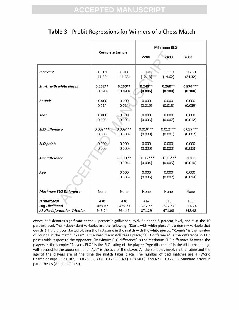
ACC

EPTE

D M

ANU

SCR

IPT

ACCEPTED MANUSCRIPT

Table 3 - Probit Regressions for Winners of a Chess Match

Complete Sample

Minimum ELO 2200 2400

2600

Intercept -0.101 -0.100 -0.120 -0.130 -0.280 (11.50) (11.66) (12.18) (14.62) (24.32) Starts with white pieces 0.202** 0.200** 0.240** 0.260** 0.570*** (0.090) (0.090) (0.096) (0.109) (0.188) Rounds -0.000 0.000 0.000 0.000 0.000 (0.014) (0.014) (0.016) (0.018) (0.039) Year -0.000 0.000 0.000 0.000 0.000 (0.005) (0.005) (0.006) (0.007) (0.012) ELO difference 0.008*** 0.009*** 0.010*** 0.012*** 0.015*** (0.000) (0.000) (0.000) (0.001) (0.002) ELO points 0.000 0.000 0.000 0.000 0.000 (0.000) (0.000) (0.000) (0.000) (0.003) Age difference -0.011** -0.012*** -0.015*** -0.001 (0.004) (0.004) (0.005) (0.010) Age 0.000 0.000 0.000 0.000 (0.006) (0.006) (0.007) (0.014) Maximum ELO Difference

None None None None None

N (matches) 438 438 414 315 116 Log-Likelihood -465.62 -459.23 -427.65 -327.54 -116.24 Akaike Information Criterion 943.24 934.45 871.29 671.08 248.48

Notes: *** denotes significant at the 1 percent significance level, ** at the 5 percent level, and * at the 10 percent level. The independent variables are the following: “Starts with white pieces” is a dummy variable that equals 1 if the player started playing the first game in the match with the white pieces; “Rounds” is the number of rounds in the match; “Year” is the year the match takes place; “ELO difference” is the difference in ELO points with respect to the opponent; “Maximum ELO difference” is the maximum ELO difference between the players in the sample; “Player’s ELO” is the ELO rating of the player; “Age difference” is the difference in age with respect to the opponent, and “Age” is the age of the player. All the variables involving the rating and the age of the players are at the time the match takes place. The number of tied matches are 4 (World Championships), 17 (Elite, ELO>2600), 33 (ELO>2500), 49 (ELO>2400), and 67 (ELO>2200). Standard errors in parentheses (Graham (2015)).

ACC

EPTE

D M

ANU

SCR

IPT

ACCEPTED MANUSCRIPT

Figure 1. The number of matches in each category are reported in parentheses. The p-values of the proportions

Chi-square tests are 0.04 (All matches), 0.02 (Elite matches), 0.68 (Non-Elite matches), 0.004 (World

Championship matches) and 0.79 (Non-World Championship matches).

Figure 2. Matches are sorted by the difference in ELO ratings into four intervals (quartiles). The endpoint of the

first interval is chosen so that it cuts off the lowest 25% of the sorted ELO differences. Similarly, the other

endpoints cut off the 50%, 75% and 100%, respectively. The intervals are reported below each quartile. The

number of matches in each quartile is 61, 42, 46 and 48 respectively. The differences in the number of matches

across the intervals comes from the discreetness of the ELO ratings, which until the late 1999 moved in

increments of 5 points.

ACC

EPTE

D M

ANU

SCR

IPT

ACCEPTED MANUSCRIPT

JPUBE‐D‐14‐00799 

HIGHLIGHTS  

“Cognitive Performance in Competitive Environments: Evidence from a Natural Experiment” 

 Julio González‐Díaz and Ignacio Palacios‐Huerta 

  

 

This paper studies cognitive performance in a high‐stakes competitive environment.   A natural experiment randomly allocates emotional states across experienced professionals.   The evidence is consistent with the hypothesis that psychological factors affect performance.