Embed Size (px)
Citation preview

Univerza v Ljubljani Fakulteta za gradbeništvo in geodezijo
Jamova 2 1000 Ljubljana, Slovenija telefon (01) 47 68 500 faks (01) 42 50 681 [email protected]
Kandidat:
Uroš Bohinc
Prilagodljivo modeliranje ploskovnih konstrukcij
Doktorska disertacija št. 212
Podiplomski program Gradbeništvo Konstrukcijska smer
Mentor: prof. dr. Boštjan Brank Somentor: prof. dr. Adnan Ibrahimbegović
Ljubljana, 5. 5. 2011
Univerza v Ljubljani
Fakulteta za gradbeništvo in geodezijo
Kandidat:
UROŠ BOHINC, univ. dipl. inž. fiz.
PRILAGODLJIVO MODELIRANJE PLOSKOVNIH
KONSTRUKCIJ
Doktorska disertacija štev.: 212
ADAPTIVE MODELING OF PLATE STRUCTURES
Doctoral thesis No.: 212
Soglasje k temi doktorske disertacije je dal Senat Univerze v Ljubljani
na 3. seji 20. novembra 2005 in za mentorja imenoval doc. dr. Boštjana Branka, za somentorja pa prof. dr. Adnana Ibrahimbegovića.
Na 27. seji 3. decembra 2009 je Komisija za doktorski študij dala soglasje k pisanju disertacije v angleškem jeziku.
Ljubljana, 5. maj 2011
PODIPLOMSKI ŠTUDIJ GRADBENIŠTVA DOKTORSKI ŠTUDIJ


Univerza v Ljubljani
Fakulteta za gradbeništvo in geodezijo
Komisijo za oceno ustreznosti teme doktorske disertacije v sestavi - doc. dr. Boštjan Brank, - prof. dr. Adnan Ibrahimbegović, ENS Cachan, - izr. prof. dr. Jože Korelc, - doc. dr. Tomaž Rodič, UL NTF
je imenoval Senat Fakultete za gradbeništvo in geodezijo na 19. redni seji
dne 20. aprila 2005.
Komisijo za oceno doktorske disertacije v sestavi - prof. dr. Ivica Kožar, Sveučilište u Rijeci, Grañevinski
fakultet, - prof. dr. Miran Saje, - izr. prof. dr. Marko Kegl, UM FS
je imenoval Senat Fakultete za gradbeništvo in geodezijo na 17. redni seji
dne 26. januarja 2011.
Komisijo za zagovor doktorske disertacije v sestavi
- prof. dr. Matjaž Mikoš, dekan UL FGG, predsednik, - prof. dr. Ivica Kožar, Sveučilište u Rijeci, Grañevinski
fakultet, - prof. dr. Miran Saje, - izr. prof. dr. Marko Kegl, UM FS, - prof. dr. Boštjan Brank, mentor, - prof. dr. Adnan Ibrahimbegović, ENS Cachan, somentor.
je imenoval Senat Fakultete za gradbeništvo in geodezijo na 20. redni seji
dne 20. aprila 2011.

Univerza v Ljubljani
Fakulteta za gradbeništvo in geodezijo
IZJAVA O AVTORSTVU
Podpisani UROŠ BOHINC, univ. dipl. inž. fiz., izjavljam, da sem avtor doktorske disertacije z naslovom: »PRILAGODLJIVO MODELIRANJE PLOSKOVNIH
KONSTRUKCIJ «.
Ljubljana, 5. maj 2011 ………………………………..
(podpis)


Bohinc, U. 2011. Prilagodljivo modeliranje ploskovnih konstrukcij
Doktorska disertacija. Ljubljana, UL, Fakulteta za gradbenistvo in geodezijo, Konstrukcijska smer vii
BIBLIOGRAPHIC-DOCUMENTARY INFORMATION
UDC 519.61/.64:624.04:624.073(043.3)Author: Uros BohincSupervisor: assoc. prof. Bostjan BrankCo-supervisor: prof. Adnan IbrahimbegovicTitle: Adaptive analysis of plate structuresNotes:
289 p., 8 tab., 185 fig., 332 eq.Key words: structures, plates, plate models, finite element method,
discretization error, model error, adaptivity
AbstractThe thesis deals with adaptive finite element modeling of plate structures. The finite elementmodeling of plates has grown to a mature research topic, which has contributed significantly tothe development of the finite element method for structural analysis due to its complexity andinherently specific issues. At present, several validated plate models and corresponding familiesof working and efficient finite elements are available, offering a sound basis for an engineer tochoose from. In our opinion, the main problems in the finite modeling of plates are nowadaysrelated to the adaptive modeling. Adaptive modeling should reach much beyond standarddiscretization (finite element mesh) error estimates and related mesh (discretization) adaptivity.It should also include model error estimates and model adaptivity, which should provide themost appropriate mathematical model for a specific region of a structure. Thus in this work westudy adaptive modeling for the case of plates.The primary goal of the thesis is to provide some answers to the questions related to the keysteps in the process of adaptive modeling of plates. Since the adaptivity depends on reliableerror estimates, a large part of the thesis is related to the derivation of computational proceduresfor discretization error estimates as well as model error estimates. A practical comparison ofsome of the established discretization error estimates is made. Special attention is paid to whatis called equilibrated residuum method, which has a potential to be used both for discretizationerror and model error estimates. It should be emphasized that the model error estimates arequite hard to obtain, in contrast to the discretization error estimates. The concept of modeladaptivity for plates is in this work implemented on the basis of equilibrated residuum methodand hierarchic family of plate finite element models.The finite elements used in the thesis range from thin plate finite elements to thick plate finiteelements. The latter are based on a newly derived higher order plate theory, which includesthrough the thickness stretching. The model error is estimated by local element-wise compu-tations. As all the finite elements, representing the chosen plate mathematical models, arere-derived in order to share the same interpolation bases, the difference between the local com-putations can be attributed mainly to the model error. This choice of finite elements enableseffective computation of the model error estimate and improves the robustness of the adaptivemodeling. Thus the discretization error can be computed by an independent procedure.Many numerical examples are provided as an illustration of performance of the derived plateelements, the derived discretization error procedures and the derived modeling error procedure.Since the basic goal of modeling in engineering is to produce an effective model, which willproduce the most accurate results with the minimum input data, the need for the adaptivemodeling will always be present. In this view, the present work is a contribution to the finalgoal of the finite element modeling of plate structures: a fully automatic adaptive procedurefor the construction of an optimal computational model (an optimal finite element mesh and anoptimal choice of a plate model for each element of the mesh) for a given plate structure.
viiiBohinc, U. 2011. Adaptive modeling of plate structures
Doctoral thesis. Cachan, ENS Cachan, LMT
BIBLIOGRAFSKO-DOKUMENTACIJSKA STRAN
UDK 519.61/.64:624.04:624.073(043.3)Avtor: Uros BohincMentor: izr. prof. dr. Bostjan BrankSomentor: prof. dr. Adnan IbrahimbegovicNaslov: Prilagodljivo modeliranje ploskovnih konstrukcijObseg in oprema:
289 str., 8 pregl., 185 sl., 332 en.Kljucne besede: konstrukcije, metoda koncnih elementov, plosce, mod-
eli plosc, napaka diskretizacije, modelska napaka, pri-lagodljivost
IzvlecekV disertaciji se ukvarjamo z razlicnimi vidiki modeliranja ploskovnih konstrukcij s koncnimielementi. Modeliranje plosc je nekoliko specificno in je zaradi kompleksnosti in pojavov, kijih opisuje, bistveno prispevalo k razvoju same metode koncnih elementov. Danes je na voljovec uveljavljenih modelov plosc in pripadajocih koncnih elementov, ki uporabniku nudijo sirokomnozico moznosti, iz katere lahko izbira. Prav siroka moznost izbire predstavlja tudi najvecjotezavo, saj je tezje dolociti, kateri model je primernejsi in tudi, katera mreza koncnih elementovje za dan problem optimalna.Glavni cilj disertacije je raziskati kljucne korake v procesu prilagodljivega modeliranja plosc,ki omogoca samodejno dolocitev optimalnega modela za dan problem. Ker je prilagodljivomodeliranje odvisno od zanesljivih ocen napak, je vecji del disertacije posvecen metodam zaizracun diskretizacijske in modelske napake. Na prakticnih primerih smo preucili nekaj najboljuveljavljenih metod za oceno napake. V nasprotju z ocenami napake diskretizacije, je modelskonapako mnogo tezje dolociti. Posebna pozornost je bila zato namenjena metodi uravnotezenjarezidualov, ki ima potencial tudi na podrocju ocene modelske napake. V tem smislu to delopredstavlja pomemben prispevek k podrocju racunanja modelske napake za plosce.Koncept prilagodljivega modeliranja ploskovnih konstrukcij je bil preskusen na hierarhicnidruzini koncnih elementov za plosce - od tankih plosc do modelov visjega reda, ki upostevajodeformacije po debelini. Ravno dobro vzpostavljena hierarhija v druzini koncnih elementov seje pokazala za kljucno pri zanesljivi oceni modelske napake.Prilagodljivo modeliranje ploskovnih konstrukcije je bilo preskuseno na nekaj zahtevnejsihprimerih. Obmocje je bilo najprej modeliranjo z najbolj grobim modelom na sorazmerno redkimrezi. Z uporabo informacije o napaki zacetnega izracuna je bil zgrajen nov model. Primerjavaizracuna na novem modelu z zacetnim racunom je pokazala, da je predlagan nacin prilagodljivegamodeliranja sposoben nadzorovati porazdelitev napake, kakor tudi zajeti vse pomembnejse po-jave, ki so znacilni za modeliranje plosc.

Bohinc, U. 2011. Prilagodljivo modeliranje ploskovnih konstrukcij
Doktorska disertacija. Ljubljana, UL, Fakulteta za gradbenistvo in geodezijo, Konstrukcijska smer ix
INFORMATION BIBLIOGRAPHIQUE-DOCUMENTAIRE
CDU 519.61/.64:624.04:624.073(043.3)Auteur: Uros BohincDirecteur de these: prof. Bostjan BrankCo-directeur de these: prof. Adnan IbrahimbegovicTitre: Modelisation adaptives des structuresNotes:
289 p., 8 tab., 185 fig., 332 eq.Mots cles: structures, plaques, modele de plaques, methode
elements finis, erreur de discretisation, erreur de mod-elisation, adaptativite
Resume
Le rapport de these traite la modelisation adaptative des plaques par la methode deselements finis. Le domaine de recherche sur la methode des elements finis de plaques aatteint une certaine maturite et a contribue d’une maniere significative au developpementde la methode des elements finis dans un sens plus large, en apportant les reponses a desproblemes tres specifiques et complexes. A present, on dispose de nombreux modeles deplaques et des formulations d’elements finis correspondantes efficaces et operationnelles,qui offrent a l’ingenieur une bonne base pour bien choisir la solution adaptee. A notreavis, les principaux problemes ouverts pour la modelisation des plaques par elements finissont aujourd’hui lies a la modelisation adaptative. Une modelisation adaptative devraitaller au-dela de l’estimation d’erreurs dues a la discretisation standard (maillage elementsfinis) et de l’adaptivite de maillages. Elle devrait inclure aussi l’estimation d’erreur dueau modele et l’adaptativite de modeles, afin de disposer d’un modele le mieux adaptepour chaque sous-domaine de la structure.
L’objectif principal de la these est de repondre a des questions liees aux etapes cled’un processus de l’adaptation de modeles de plaques. Comme l’adaptativite depend desestimateurs d’erreurs fiables, une part importante du rapport est dediee au developpementdes methodes numeriques pour les estimateurs d’erreurs aussi bien dues a la discretisationqu’au choix du modele. Une comparaison des estimateurs d’erreurs de discretisation d’unpoint de vue pratique est presentee. Une attention particuliere est pretee a la methode deresiduels equilibres (en anglais, ”equilibrated residual method”), laquelle est potentielle-ment applicable aux estimations des deux types d’erreurs, de discretisation et de modele.Il faut souligner que, contrairement aux estimateurs d’erreurs de discretisation, les esti-mateurs d’erreur de modele sont plus difficiles a elaborer. Le concept de l’adaptativite demodeles pour les plaques est implemente sur la base de la methode de residuels equilibreset de la famille hierararchique des elements finis de plaques. Les elements finis derivesdans le cadre de la these, comprennent aussi bien les elements de plaques minces et queles elements de plaques epaisses. Ces derniers sont formules en s’appuyant sur une theorienouvelle de plaque, integrant aussi les effets d’etirement le long de l’epaisseur. Les erreursde modele sont estimees via des calculs element par element. Les erreurs de discretisationet de modele sont estimees d’une maniere independante, ce qui rend l’approche tres ro-buste et facile a utiliser. Les methodes developpees sont appliquees sur plusieurs exem-ples numeriques. Les travaux realises dans le cadre de la these representent plusieurscontributions qui visent l’objectif final de la modelisation adaptative, ou une procedurecompletement automatique permettrait de faire un choix optimal du modele de plaquespour chaque element de la structure.
xBohinc, U. 2011. Adaptive modeling of plate structures
Doctoral thesis. Cachan, ENS Cachan, LMT
ZAHVALA
Za nesebicno pomoc in vso spodbudo se zahvaljujem mentorjema, prof. dr. BostjanuBranku in prof. dr. Adnanu Ibrahimbegovicu. Na prehojeno pot se oziram z zadovoljstvom,da sem imel priloznost in cast delati z vama.
Zahvaljujem se izr. prof. dr. Andrazu Legatu, ki me je podpiral ves cas studija, tuditakrat, ko to ni bilo lahko.
Vesel sem, da sem pri studiju vztrajal, saj sicer ne bi spoznal takih prijateljev, kot staJaka in Damijan. Ceprav se nisva spoznala med studijem, pa si prav takrat pokazal svojosrcnost in prijateljstvo. Vlado, hvala ti, ker si znal biti in ostati prijatelj do konca.
Brez svojih najblizjih, mojih starsev in starsev moje zene tega dela danes gotovo ne bibilo. Ob dolgi in zaviti poti sem bil vedno delezen vase nesebicne podpore in pomoci, zakar sem vam iskreno hvalezen.
Moja druzina, Polona, Blaz in Tine so sodelovali pri tem delu bolj, kot sem si upalpredstavljati na zacetku. Neskoncno zaupanje in podporo, ki sem ju dobil od vas, lahkodobis le od nekoga, ki te ima resnicno rad.
To delo posvecam tebi, Klemen.
Bohinc, U. 2011. Prilagodljivo modeliranje ploskovnih konstrukcij
Doktorska disertacija. Ljubljana, UL, Fakulteta za gradbenistvo in geodezijo, Konstrukcijska smer xi
Contents
1 Introduction 1
1.1 Motivation . . . . . . . . . . . . . . . . . . . . . . . . . . . . . . . . . . . . 1
1.1.1 Verification and Validation . . . . . . . . . . . . . . . . . . . . . . . 2
1.1.2 Discretization . . . . . . . . . . . . . . . . . . . . . . . . . . . . . . 2
1.1.3 Model error. Discretization error. The optimal model. . . . . . . . . 3
1.1.4 Adaptive modeling. Error estimates and indicators . . . . . . . . . 5
1.2 Goals of the thesis . . . . . . . . . . . . . . . . . . . . . . . . . . . . . . . 6
1.3 Outline of the thesis . . . . . . . . . . . . . . . . . . . . . . . . . . . . . . 7
2 Thin plates: theory and finite element formulations 9
2.1 Introduction . . . . . . . . . . . . . . . . . . . . . . . . . . . . . . . . . . . 9
2.2 Theory . . . . . . . . . . . . . . . . . . . . . . . . . . . . . . . . . . . . . . 9
2.2.1 Governing equations . . . . . . . . . . . . . . . . . . . . . . . . . . 9
2.2.2 Further details of the Kirchhoff model . . . . . . . . . . . . . . . . 19
2.3 Finite elements . . . . . . . . . . . . . . . . . . . . . . . . . . . . . . . . . 26
2.3.1 Preliminary considerations . . . . . . . . . . . . . . . . . . . . . . . 26
2.3.2 An overview of thin plate elements . . . . . . . . . . . . . . . . . . 29
2.3.3 Natural coordinate systems . . . . . . . . . . . . . . . . . . . . . . 30
2.3.4 Conforming triangular element . . . . . . . . . . . . . . . . . . . . 37
2.3.5 Discrete Kirchhoff elements . . . . . . . . . . . . . . . . . . . . . . 41
2.4 Examples . . . . . . . . . . . . . . . . . . . . . . . . . . . . . . . . . . . . 50
2.4.1 Uniformly loaded simply supported square plate . . . . . . . . . . . 51
2.4.2 Uniformly loaded clamped square plate . . . . . . . . . . . . . . . . 53
2.4.3 Uniformly loaded clamped circular plate . . . . . . . . . . . . . . . 54
2.4.4 Uniformly loaded hard simply supported skew plate . . . . . . . . . 70
2.5 Chapter summary and conclusions . . . . . . . . . . . . . . . . . . . . . . . 75
3 Moderately thick plates: theory and finite element formulations 77

xiiBohinc, U. 2011. Adaptive modeling of plate structures
Doctoral thesis. Cachan, ENS Cachan, LMT
3.1 Introduction . . . . . . . . . . . . . . . . . . . . . . . . . . . . . . . . . . . 77
3.2 Theory . . . . . . . . . . . . . . . . . . . . . . . . . . . . . . . . . . . . . . 78
3.2.1 Governing equations . . . . . . . . . . . . . . . . . . . . . . . . . . 78
3.2.2 Strong form . . . . . . . . . . . . . . . . . . . . . . . . . . . . . . . 82
3.2.3 Weak form . . . . . . . . . . . . . . . . . . . . . . . . . . . . . . . . 85
3.2.4 Boundary layer and singularities . . . . . . . . . . . . . . . . . . . . 86
3.3 Finite elements . . . . . . . . . . . . . . . . . . . . . . . . . . . . . . . . . 89
3.3.1 Elements with cubic interpolation of displacement . . . . . . . . . . 92
3.3.2 Elements with incompatible modes . . . . . . . . . . . . . . . . . . 95
3.4 Examples . . . . . . . . . . . . . . . . . . . . . . . . . . . . . . . . . . . . 97
3.4.1 Uniformly loaded simply supported square plate . . . . . . . . . . . 97
3.4.2 Uniformly loaded simply supported free square plate . . . . . . . . 98
3.4.3 Uniformly loaded simply supported skew plate . . . . . . . . . . . . 100
3.4.4 Uniformly loaded soft simply supported L-shaped plate . . . . . . . 101
3.5 Chapter summary and conclusions . . . . . . . . . . . . . . . . . . . . . . . 119
4 Thick plates: theory and finite element formulations 121
4.1 Introduction . . . . . . . . . . . . . . . . . . . . . . . . . . . . . . . . . . . 121
4.2 Theory . . . . . . . . . . . . . . . . . . . . . . . . . . . . . . . . . . . . . . 122
4.2.1 Governing equations . . . . . . . . . . . . . . . . . . . . . . . . . . 122
4.2.2 Principle of virtual work . . . . . . . . . . . . . . . . . . . . . . . . 124
4.3 Finite elements . . . . . . . . . . . . . . . . . . . . . . . . . . . . . . . . . 128
4.3.1 Higher-order plate elements . . . . . . . . . . . . . . . . . . . . . . 128
4.4 Hierarchy of derived plate elements . . . . . . . . . . . . . . . . . . . . . . 133
4.5 Examples . . . . . . . . . . . . . . . . . . . . . . . . . . . . . . . . . . . . 136
4.5.1 Uniformly loaded simply supported square plate . . . . . . . . . . . 136
4.5.2 Uniformly loaded soft simply supported L-shaped plate . . . . . . . 137
4.5.3 Simply supported square plate with load variation . . . . . . . . . . 138
4.6 Chapter summary and conclusions . . . . . . . . . . . . . . . . . . . . . . . 145
5 Discretization error estimates 147
5.1 Introduction. Classification of error estimates . . . . . . . . . . . . . . . . 147
5.2 Definitions. Linear elasticity as a model problem . . . . . . . . . . . . . . . 149
5.3 Recovery based error estimates . . . . . . . . . . . . . . . . . . . . . . . . 151
5.3.1 Lumped projection . . . . . . . . . . . . . . . . . . . . . . . . . . . 153

Bohinc, U. 2011. Prilagodljivo modeliranje ploskovnih konstrukcij
Doktorska disertacija. Ljubljana, UL, Fakulteta za gradbenistvo in geodezijo, Konstrukcijska smer xiii
5.3.2 Superconvergent patch recovery (SPR) . . . . . . . . . . . . . . . . 153
5.4 Residual based error estimates . . . . . . . . . . . . . . . . . . . . . . . . . 155
5.4.1 Explicit . . . . . . . . . . . . . . . . . . . . . . . . . . . . . . . . . 155
5.4.2 Implicit . . . . . . . . . . . . . . . . . . . . . . . . . . . . . . . . . 158
5.5 Illustration of SPR and EqR methods on 1D problem . . . . . . . . . . . . 169
5.6 Chapter summary and conclusions . . . . . . . . . . . . . . . . . . . . . . . 172
6 Discretization error for DK and RM elements 175
6.1 Introduction . . . . . . . . . . . . . . . . . . . . . . . . . . . . . . . . . . . 175
6.2 Discretization error for DK elements . . . . . . . . . . . . . . . . . . . . . 176
6.2.1 Discrete approximation for error estimates . . . . . . . . . . . . . . 176
6.2.2 Formulation of local boundary value problem . . . . . . . . . . . . . 179
6.2.3 Enhanced approximation for the local computations . . . . . . . . . 183
6.2.4 Numerical examples . . . . . . . . . . . . . . . . . . . . . . . . . . 185
6.2.5 An example of adaptive meshing . . . . . . . . . . . . . . . . . . . 189
6.3 Discretization error for RM elements . . . . . . . . . . . . . . . . . . . . . 201
6.4 Chapter summary and conclusions . . . . . . . . . . . . . . . . . . . . . . . 201
7 Model error concept 203
7.1 Introduction . . . . . . . . . . . . . . . . . . . . . . . . . . . . . . . . . . . 203
7.2 Model error indicator based on local EqR computations . . . . . . . . . . . 205
7.2.1 Definition of model error indicator . . . . . . . . . . . . . . . . . . 205
7.2.2 Construction of equilibrated boundary tractions for local problems . 210
7.3 Chapter summary and conclusions . . . . . . . . . . . . . . . . . . . . . . . 216
8 Model error indicator for DK elements 219
8.1 Introduction . . . . . . . . . . . . . . . . . . . . . . . . . . . . . . . . . . . 219
8.2 Model error indicator . . . . . . . . . . . . . . . . . . . . . . . . . . . . . . 221
8.2.1 Regularization . . . . . . . . . . . . . . . . . . . . . . . . . . . . . . 223
8.2.2 The local problems with RM plate element . . . . . . . . . . . . . . 224
8.2.3 Computation of the model error indicator . . . . . . . . . . . . . . 226
8.2.4 Numerical examples . . . . . . . . . . . . . . . . . . . . . . . . . . 226
8.3 Chapter summary and conclusions . . . . . . . . . . . . . . . . . . . . . . . 241
9 Conclusions 243

xivBohinc, U. 2011. Adaptive modeling of plate structures
Doctoral thesis. Cachan, ENS Cachan, LMT
10 Razsirjeni povzetek 247
10.1 Motivacija . . . . . . . . . . . . . . . . . . . . . . . . . . . . . . . . . . . . 247
10.1.1 Verifikacija in validacija . . . . . . . . . . . . . . . . . . . . . . . . 248
10.1.2 Prilagodljivo modeliranje - optimalni model . . . . . . . . . . . . . 248
10.1.3 Napaka diskretizacije, modelska napaka . . . . . . . . . . . . . . . . 250
10.2 Cilji . . . . . . . . . . . . . . . . . . . . . . . . . . . . . . . . . . . . . . . 251
10.3 Zgradba naloge . . . . . . . . . . . . . . . . . . . . . . . . . . . . . . . . . 252
10.4 Plosce . . . . . . . . . . . . . . . . . . . . . . . . . . . . . . . . . . . . . . 253
10.4.1 Tanke plosce . . . . . . . . . . . . . . . . . . . . . . . . . . . . . . . 253
10.4.2 Srednje debele plosce . . . . . . . . . . . . . . . . . . . . . . . . . . 261
10.4.3 Debele plosce . . . . . . . . . . . . . . . . . . . . . . . . . . . . . . 268
10.5 Ocene napak . . . . . . . . . . . . . . . . . . . . . . . . . . . . . . . . . . . 273
10.5.1 Napaka diskretizacije . . . . . . . . . . . . . . . . . . . . . . . . . . 273
10.5.2 Ocena modelske napake . . . . . . . . . . . . . . . . . . . . . . . . 278
10.6 Zakljucek . . . . . . . . . . . . . . . . . . . . . . . . . . . . . . . . . . . . 281
List of Figures
2.2.1 Mathematical idealization of a plate, · · · . . . . . . . . . . . . . . . . . . 10
2.2.2 Stress resultants - shear forces and moments - on a midsurface differential
element . . . . . . . . . . . . . . . . . . . . . . . . . . . . . . . . . . . . 13
2.2.3 Rotations at the boundary . . . . . . . . . . . . . . . . . . . . . . . . . . 14
2.2.4 Boundary coordinate system, moments and test rotations . . . . . . . . 17
2.2.5 Concentrated corner force at node I . . . . . . . . . . . . . . . . . . . . . 19
2.2.6 To the definition of a corner force in (2.2.47) . . . . . . . . . . . . . . . . 19
2.2.7 Plate boundary traction loading · · · . . . . . . . . . . . . . . . . . . . . 20
2.2.8 Definition of a polar coordinate system (r, ϕ) at the corner . . . . . . . . 24
2.3.1 Problem domain Ω and its boundary Γ (left), finite element discretization
Ωeh, Ωh and patch of elements ΩPi
h around node i (right) . . . . . . . . . 28
2.3.2 Bi-unit element Ω in coordinate system (ξ,η) . . . . . . . . . . . . . . . 31
2.3.3 Quadrilateral element with the alternate shading between the coordinate
lines of the quadrilateral natural coordinate system . . . . . . . . . . . . 33
2.3.4 Triangular (area) coordinates . . . . . . . . . . . . . . . . . . . . . . . . 33

Bohinc, U. 2011. Prilagodljivo modeliranje ploskovnih konstrukcij
Doktorska disertacija. Ljubljana, UL, Fakulteta za gradbenistvo in geodezijo, Konstrukcijska smer xv
2.3.5 Triangular element with the alternate shading between the coordinate
lines ζi = const. of triangular coordinate system . . . . . . . . . . . . . . 35
2.3.6 To the definition of eccentricity parameter µ12 = 2e1/l12 . . . . . . . . . 37
2.3.7 Triangular Argyris plate element - ARGY . . . . . . . . . . . . . . . . . 38
2.3.8 Hierarchical shape functions . . . . . . . . . . . . . . . . . . . . . . . . . 42
2.3.9 Euler-Bernoulli beam element . . . . . . . . . . . . . . . . . . . . . . . . 42
2.3.10 Hermite shape functions . . . . . . . . . . . . . . . . . . . . . . . . . . . 43
2.3.11 Node and side numbering in (2.3.64) . . . . . . . . . . . . . . . . . . . . 45
2.3.12 Triangular DK plate element - DK . . . . . . . . . . . . . . . . . . . . . 46
2.3.13 Hierarchic shape functions of the triangular DK plate element . . . . . . 48
2.3.14 Hierarchic shape functions of the quadrilateral DK plate element . . . . 49
2.4.1 Designation of boundary conditions and loads . . . . . . . . . . . . . . . 50
2.4.2 Problem definition and geometry for the uniformly loaded simply sup-
ported square plate (t/a=1/1000) . . . . . . . . . . . . . . . . . . . . . . 51
2.4.7 Problem definition and geometry for the uniformly loaded clamped square
plate (t/a=1/1000) . . . . . . . . . . . . . . . . . . . . . . . . . . . . . . 53
2.4.12 Clamped circular plate with uniform load (t/R=1/500) . . . . . . . . . . 55
2.4.3 Reference solution of the uniformly loaded simply supported square plate
· · · . . . . . . . . . . . . . . . . . . . . . . . . . . . . . . . . . . . . . . . 57
2.4.4 FE solution of the uniformly loaded simply supported square plate with
Argyris plate element . . . . . . . . . . . . . . . . . . . . . . . . . . . . 58
2.4.5 Finite element solution of the uniformly loaded simply supported square
plate with DK plate elements . . . . . . . . . . . . . . . . . . . . . . . . 59
2.4.6 Comparison of the convergence of FE solutions for the uniformly loaded
simply supported square plate . . . . . . . . . . . . . . . . . . . . . . . 60
2.4.8 Reference solution of the uniformly loaded clamped square plate , · · · . . 61
2.4.9 FE solution of the uniformly loaded clamped square plate with Argyris
plate element . . . . . . . . . . . . . . . . . . . . . . . . . . . . . . . . . 62
2.4.10 FE solution of the uniformly loaded clamped square plate with DK plate
elements . . . . . . . . . . . . . . . . . . . . . . . . . . . . . . . . . . . . 63
2.4.11 Comparison of the convergence of FE solutions for the uniformly loaded
clamped square plate . . . . . . . . . . . . . . . . . . . . . . . . . . . . 64
2.4.13 Reference solution of the uniformly loaded clamped circular plate , · · · . 65
2.4.14 The sequence of meshes used for the finite element solution of uniformly
loaded clamped circular plate . . . . . . . . . . . . . . . . . . . . . . . . 66
2.4.15 FE solution of the uniformly loaded clamped circular plate with Argyris
plate element . . . . . . . . . . . . . . . . . . . . . . . . . . . . . . . . . 67
xviBohinc, U. 2011. Adaptive modeling of plate structures
Doctoral thesis. Cachan, ENS Cachan, LMT
2.4.16 FE solution of the uniformly loaded clamped circular plate with DK plate
elements . . . . . . . . . . . . . . . . . . . . . . . . . . . . . . . . . . . . 68
2.4.17 Comparison of the convergence of FE solutions for the uniformly loaded
clamped circular plate . . . . . . . . . . . . . . . . . . . . . . . . . . . . 69
2.4.18 Problem definition and geometry for the uniformly loaded simply sup-
ported skew plate (t/a=100) . . . . . . . . . . . . . . . . . . . . . . . . . 70
2.4.19 Reference solution of the uniformly loaded simply supported skew plate
, · · · . . . . . . . . . . . . . . . . . . . . . . . . . . . . . . . . . . . . . . 71
2.4.20 FE solution of the uniformly loaded simply supported skew plate with
ARGY element, · · · . . . . . . . . . . . . . . . . . . . . . . . . . . . . . 72
2.4.21 FE solution of the uniformly loaded simply supported skew plate with
DK elements, · · · . . . . . . . . . . . . . . . . . . . . . . . . . . . . . . . 73
2.4.22 Comparison of the convergence of FE solutions for the uniformly loaded
simply supported skew plate . . . . . . . . . . . . . . . . . . . . . . . . 74
3.3.1 To the computation of the nodal shear γh,I from (3.3.18) . . . . . . . . . 94
3.3.2 Quadrilateral plate element P3Q with cubic displacement interpolation . 96
3.4.1 Problem definition and geometry for the uniformly loaded hard-soft sim-
ply supported square plate (t/a=1/10) . . . . . . . . . . . . . . . . . . . 97
3.4.6 Problem definition and geometry for the uniformly loaded hard simply
supported-free square plate (t/a=10) . . . . . . . . . . . . . . . . . . . . 99
3.4.11 Problem definition and geometry for the uniformly loaded soft simply
supported skew plate (t/a=10) . . . . . . . . . . . . . . . . . . . . . . . 100
3.4.16 Problem definition and geometry for the uniformly loaded soft simply
supported L-shaped plate (t/a=10) . . . . . . . . . . . . . . . . . . . . . 101
3.4.2 Reference solution of the uniformly loaded hard-soft simply supported
square plate with legend also valid for Figures 3.4.4 and 3.4.3 . . . . . . 103
3.4.3 FE solution of the uniformly loaded hard-soft simply supported square
plate with PI plate elements . . . . . . . . . . . . . . . . . . . . . . . . . 104
3.4.4 FE solution of the uniformly loaded hard-soft simply supported square
plate with P3 plate elements (mesh as in Figure 3.4.3) . . . . . . . . . . 105
3.4.5 Comparison of the convergence of FE solutions for the uniformly loaded
hard-soft simply supported square plate . . . . . . . . . . . . . . . . . . 106
3.4.7 Reference solution of the uniformly loaded hard simply supported-free
square plate with legend also valid for Figures 3.4.9 and 3.4.8 . . . . . . 107
3.4.8 FE solutions of the uniformly loaded hard simply supported-free square
plate with PI plate elements . . . . . . . . . . . . . . . . . . . . . . . . . 108
Bohinc, U. 2011. Prilagodljivo modeliranje ploskovnih konstrukcij
Doktorska disertacija. Ljubljana, UL, Fakulteta za gradbenistvo in geodezijo, Konstrukcijska smer xvii
3.4.9 FE solutions of the uniformly loaded hard simply supported-free square
plate with P3 plate elements (mesh as in Figure 3.4.8) . . . . . . . . . . 109
3.4.10 Comparison of the convergence of FE solutions for the uniformly loaded
hard simply supported-free square plate . . . . . . . . . . . . . . . . . . 110
3.4.12 Reference solution of the uniformly loaded soft simply supported skew
plate with legend also valid for Figures 3.4.14 and 3.4.13 . . . . . . . . . 111
3.4.13 FE solution of the uniformly loaded soft simply supported skew plate
with PI plate elements . . . . . . . . . . . . . . . . . . . . . . . . . . . . 112
3.4.14 FE solution of the uniformly loaded soft simply supported skew plate
with P3 plate elements (mesh as in Figure 3.4.13) . . . . . . . . . . . . . 113
3.4.15 Comparison of the convergence of FE solutions for the uniformly loaded
soft simply supported skew plate . . . . . . . . . . . . . . . . . . . . . . 114
3.4.17 Reference solution of the uniformly loaded soft simply supported L-
shaped plate with legend also valid for Figures 3.4.19 and 3.4.18 . . . . . 115
3.4.18 FE solution of the uniformly loaded soft simply supported L-shaped plate
with PI plate elements . . . . . . . . . . . . . . . . . . . . . . . . . . . . 116
3.4.19 FE solution of the uniformly loaded soft simply supported L-shaped plate
with P3 plate elements (mesh as in Figure 3.4.18) . . . . . . . . . . . . . 117
3.4.20 Comparison of the convergence of FE solutions for the uniformly loaded
soft simply supported L-shaped plate . . . . . . . . . . . . . . . . . . . 118
4.2.1 Kinematics of through-the-thickness deformation in the thick plate model 122
4.3.1 Designation of plate surfaces Ω+, Ω− and Γ . . . . . . . . . . . . . . . . 132
4.5.1 Problem definition and geometry for the uniformly loaded hard-soft sim-
ply supported square plate (t/a=1/10) . . . . . . . . . . . . . . . . . . . 136
4.5.4 Problem definition and geometry for the uniformly loaded soft simply
supported L shaped plate (t/a=1/10) . . . . . . . . . . . . . . . . . . . . 137
4.5.7 Problem definition and geometry for the simply supported square plate
with load variation (t/a=1/10 and t/b=1) . . . . . . . . . . . . . . . . . 138
4.5.2 FE solution of the uniformly loaded simply supported square plate with
PZ plate elements . . . . . . . . . . . . . . . . . . . . . . . . . . . . . . 139
4.5.3 Legend for Figures 4.5.2 . . . . . . . . . . . . . . . . . . . . . . . . . . . 140
4.5.5 FE solution of the uniformly loaded soft simply supported L shaped plate
with PZ plate elements . . . . . . . . . . . . . . . . . . . . . . . . . . . . 141
4.5.6 Legend for Figures 4.5.5 . . . . . . . . . . . . . . . . . . . . . . . . . . . 142
4.5.8 FE solution of the simply supported square plate with load variation
with PZ plate elements . . . . . . . . . . . . . . . . . . . . . . . . . . . . 143
4.5.9 Legend for Figures 4.5.8 . . . . . . . . . . . . . . . . . . . . . . . . . . . 144
xviiiBohinc, U. 2011. Adaptive modeling of plate structures
Doctoral thesis. Cachan, ENS Cachan, LMT
5.1.1 Rough classification of a-posteriori error estimates/indicators . . . . . . 149
5.3.1 SPR recovery of the enhanced stress σ∗I at node I . . . . . . . . . . . . . 155
5.4.1 Notation . . . . . . . . . . . . . . . . . . . . . . . . . . . . . . . . . . . . 159
5.4.2 Relation of tractions teΓ to their projections reI,Γ . . . . . . . . . . . . . . 163
5.4.3 Element nodal residual ReI and boundary tractions projections re
I,Γ1,2at
node I of element e . . . . . . . . . . . . . . . . . . . . . . . . . . . . . . 164
5.4.4 Continuity of boundary tractions projections reI,Γ . . . . . . . . . . . . . 164
5.4.5 Patch PI of four elements around node I . . . . . . . . . . . . . . . . . . 165
5.4.6 Representation of element nodal residuals ReI by the projections re
I,Γ . . 168
5.4.7 Boundary tractions teΓ replace the action of element projections reI,Γ . . . 168
5.5.1 One dimensional problem: hanging bar with variable cross section . . . . 169
5.5.2 Solution of the model problem with linear elements . . . . . . . . . . . . 171
5.5.3 Solution of the model problem with quadratic elements . . . . . . . . . . 171
5.5.4 Computation of enhanced stress σ∗; comparison of SPR and EqR method 172
6.2.1 Subdivision schemes for the DKT element . . . . . . . . . . . . . . . . . 184
6.2.2 Simply supported square plate under uniform loading - global energy
error estimates . . . . . . . . . . . . . . . . . . . . . . . . . . . . . . . . 186
6.2.3 Simply supported square plate under uniform loading - effectivity index
of the global energy error estimates . . . . . . . . . . . . . . . . . . . . . 187
6.2.4 Simply supported square plate under uniform loading - comparison of
relative local error estimates . . . . . . . . . . . . . . . . . . . . . . . . . 192
6.2.5 Clamped square plate under uniform loading - global energy error estimates193
6.2.6 Clamped square plate under uniform loading - effectivity index of the
global energy error estimates . . . . . . . . . . . . . . . . . . . . . . . . 193
6.2.7 Clamped square plate under uniform loading - comparison of relative
local error estimates . . . . . . . . . . . . . . . . . . . . . . . . . . . . . 194
6.2.8 Clamped circular plate under uniform loading - global energy error esti-
mates . . . . . . . . . . . . . . . . . . . . . . . . . . . . . . . . . . . . . 195
6.2.9 Clamped circular plate under uniform loading - effectivity index of the
global energy error estimates . . . . . . . . . . . . . . . . . . . . . . . . 195
6.2.10 Clamped circular plate under uniform loading - comparison of relative
local error estimates . . . . . . . . . . . . . . . . . . . . . . . . . . . . . 196
6.2.11 Morley’s skew plate under uniform loading - global energy error estimates197
6.2.12 Morley’s skew plate under uniform loading - effectivity index of the global
energy error estimates . . . . . . . . . . . . . . . . . . . . . . . . . . . . 197
6.2.13 Morley’s skew plate under uniform loading - comparison of relative local
error estimates . . . . . . . . . . . . . . . . . . . . . . . . . . . . . . . . 198

Bohinc, U. 2011. Prilagodljivo modeliranje ploskovnih konstrukcij
Doktorska disertacija. Ljubljana, UL, Fakulteta za gradbenistvo in geodezijo, Konstrukcijska smer xix
6.2.14 L-shaped plate under uniform loading - global energy error estimates . . 199
6.2.15 L-shaped plate under uniform loading - effectivity index of the global
energy error estimates . . . . . . . . . . . . . . . . . . . . . . . . . . . . 199
6.2.16 L-shaped plate under uniform loading - comparison of relative local error
estimates . . . . . . . . . . . . . . . . . . . . . . . . . . . . . . . . . . . 200
7.2.1 Local computation on a finite element domain Ωeh with Neumann bound-
ary conditions teΓe on Γe . . . . . . . . . . . . . . . . . . . . . . . . . . . 207
8.2.1 Model error indicator for thick SSSS problem for rectangular meshes . . 228
8.2.2 Model error indicator for thin SSSS problem for distorted meshes . . . . 229
8.2.3 Model error indicator for thin SSSS problem for rectangular meshes . . . 230
8.2.4 Model error indicator for thin SSSS problem for distorted meshes . . . . 231
8.2.5 Model error indicator for thick SFSF problem for rectangular meshes . . 232
8.2.6 Model error indicator for thick SFSF problem for distorted meshes . . . 233
8.2.7 Model error indicator for thin SFSF problem for rectangular meshes . . . 234
8.2.8 Model error indicator for thin SFSF problem for distorted meshes . . . . 235
8.2.9 LSHP - model error indicator . . . . . . . . . . . . . . . . . . . . . . . . 235
8.2.10 LSHP - stress resultant mxx . . . . . . . . . . . . . . . . . . . . . . . . . 236
8.2.11 LSHP - stress resultant mxy . . . . . . . . . . . . . . . . . . . . . . . . . 237
8.2.12 LSHP - stress resultant qx . . . . . . . . . . . . . . . . . . . . . . . . . . 238
8.2.13 SKEW - model error indicator . . . . . . . . . . . . . . . . . . . . . . . 238
8.2.14 SKEW - stress resultant mxx . . . . . . . . . . . . . . . . . . . . . . . . 239
8.2.15 SKEW - stress resultant mxy . . . . . . . . . . . . . . . . . . . . . . . . 239
8.2.16 SKEW - stress resultant qx . . . . . . . . . . . . . . . . . . . . . . . . . 240
List of Tables
2.1 Boundary conditions for thin plates. ∗ θn = ∂w∂s
is zero due to w = 0. . . . . 23
2.2 Critical opening angles for the Kirchhoff plate (* - the case reexamined in
this section) . . . . . . . . . . . . . . . . . . . . . . . . . . . . . . . . . . . 26
2.3 4 point triangular integration scheme for triangular finite elements (DKT) 47
2.4 4 point quadrilateral integration scheme for quadrilateral finite elements
(DKQ) . . . . . . . . . . . . . . . . . . . . . . . . . . . . . . . . . . . . . . 48

xxBohinc, U. 2011. Adaptive modeling of plate structures
Doctoral thesis. Cachan, ENS Cachan, LMT
3.1 Boundary conditions for moderately thick plates . . . . . . . . . . . . . . . 80
3.2 Leading terms of thickness expansion in (3.2.38) . . . . . . . . . . . . . . . 88
3.3 The singularity coefficients, λ1 and λ2 . . . . . . . . . . . . . . . . . . . . . 89
6.1 Comparison of errors of FE computation of the square clamped plate prob-
lem with various meshes adaptively constructed from discretization error
estimate. . . . . . . . . . . . . . . . . . . . . . . . . . . . . . . . . . . . . . 191
————————————————————————

Bohinc, U. 2011. Prilagodljivo modeliranje ploskovnih konstrukcij
Doktorska disertacija. Ljubljana, UL, Fakulteta za gradbenistvo in geodezijo, Konstrukcijska smer 1
Chapter 1
Introduction
1.1 Motivation
Understanding the behavior of structures under various loads has always been of primary
interest to man. Throughout the history the knowledge on the structural behavior was
predominantly acquired by experiments. But due to the rising complexity of the man
made structures it became obvious that it is not possible nor economical to perform the
experimental validation of all possible loading situations. It was realized that mathemati-
cal models (i.e. equations) describing physical phenomena, which would be able to predict
the structural behavior, were needed.
The models of physical phenomena have been build upon the experimental observa-
tions. The models are therefore only as accurate as the experiments are. The accuracy of
the model predictions inherently depend on the accuracy of the experimental results. The
accuracy is limited also by the computational ability of the solver, used to solve equations
of the model, which affects the level of the detail attainable in the model.
In the early days the model equations were solved analytically. Only relatively small
set of engineering problems with simple geometry and material laws were suitable to
be solved that way. Some numerical approximations were attempted but were seriously
limited by the computing power of the solver (usually human at that time). With the
advent of the modern computers the numerical approximations of the solution became
more elaborate and it became possible to numerically solve complex real life problems.
Numerical computations have nowadays become an integral part of engineering design
process. Critical design decisions are routinely made on the basis of numerical simulations.
It is therefore vitally important to clearly define the reliability and accuracy (i.e. the error)
of the computational predictions of the model.

2Bohinc, U. 2011. Adaptive modeling of plate structures
Doctoral thesis. Cachan, ENS Cachan, LMT
A numerical simulation (i.e. the mathematical model plus the numerical methods) of
a physical phenomena is accepted only when the predictions match the outcome of the
controlled experiments. The model predictions are therefore always made in the form
of measurable physical quantities. Since the engineering approach to modeling goes by
the paradigm as simple as possible and as complicated as necessary the necessary level of
complexity of a physical model is defined by the required accuracy of the model.
The difference between the controllably measured physical reality and the model pre-
dictions can be attributed to one of the two reasons: (i) the mathematical model is either
based upon the wrong assumptions and/or (ii) the equations of the mathematical model
can be solved only approximately for a given data. The error of a model prediction,
which is caused by the wrong assumptions, is usually referred to as the model error. The
approximative nature of the model results is related to the discretization error.
1.1.1 Verification and Validation
The total error of the prediction is thus always composed of a model error and a dis-
cretization error. The approximation of the exact model equations reflects itself in the
model error, while the discretization error is a consequence of the approximation in the
solution of the chosen model equations.
The concept of verification and validation (V&V) has been established to study the
model performance in terms of accuracy. Comparison of the solution of the discretized
model with the exact solution of the model is a subject of verification. The validation
usually concerns the comparison of the model predictions with the results of the experi-
ments.
1.1.2 Discretization
Mathematical model (or just model) is a mathematical idealization of a physical model
which is build upon certain assumptions and simplifications. Certain degree of abstraction
is used in the model derivation. It usually involves the concept of continuity, which
assumes that the solution is known at every point of the problem domain. Such models
cannot be solved numerically since the number of points in the problem domain is infinite.
In order to obtain a numerically solvable system, the problem has to be discretized with a
finite number of variables. A widespread method of the discretization of a given continuous
mathematical model is the finite element method (FEM). The discretization introduces a

Bohinc, U. 2011. Prilagodljivo modeliranje ploskovnih konstrukcij
Doktorska disertacija. Ljubljana, UL, Fakulteta za gradbenistvo in geodezijo, Konstrukcijska smer 3
discretization error.
The finite element method was first conceived by engineers and mathematicians to
solve the problems of linear elasticity. Nowadays, the prevalent use of the finite element
method remains in the field of linear structural mechanics. The main focus of this work
is the finite element analysis of bending of plate structures, which fits in that framework.
1.1.3 Model error. Discretization error. The optimal model.
In order to find the optimal model for the analysis of a structure behavior - in our case
elastic plate bending - the criteria have to be set first. If the accuracy is the only criteria,
the best possible model is the exact fully three-dimensional model of elastic plate bending.
Such model is of course prohibitively complicated for usual plate bending problems. The
plate model is therefore proclaimed as optimal in the engineering sense: besides the
necessary (desired) accuracy, the model must be as simple as possible.
The plates are basic structural elements and several models of their bending behavior
exist. Since the third dimension of the plate is significantly smaller than the other two, the
plate models are subject to dimensional reduction. The computational advantage of using
two-dimensional model instead of fully three-dimensional model is obvious. Although
the three-dimensional model should asymptotically converge to two-dimensional plate
model (for decreasing plate thickness), not many plate models are strictly build on the
principles of asymptotic analysis. Various important plate models are rather based on
a-priori assumptions coming from the engineering intuition. Nevertheless, a hierarchy
of such plate models can still be established with respect to the convergence to the full
three-dimensional model, [Babuska Li, 1990]. It is thus possible to form a family of
hierarchically ordered plate models - a series of models, whose solutions converge to the
exact three-dimensional solution of plate bending problem. The convergence to the exact
three-dimensional solution manifests itself, for example, in the ability to describe the
boundary layer effects, which are typical for the three-dimensional solution.
Model error
The a-priori assumptions of a plate model are usually related to its kinematics. The
kinematics of the plate strongly depends on the boundary conditions, concentrated forces
and abrupt changes in thickness or material properties. Since the kinematics changes
over the plate problem domain, so does the validity of model assumptions. The model

4Bohinc, U. 2011. Adaptive modeling of plate structures
Doctoral thesis. Cachan, ENS Cachan, LMT
is optimal only in the region, where its assumptions are valid. It is therefore clear that
the optimal model is location dependant. There is no single model which is optimal for
the whole plate domain. The plate domain should therefore be divided into regions, each
being modeled with its own optimal model. The main goal of the model adaptivity is to
identify the regions and determine the optimal model for each one of them.
The region dependent optimal model of the plate structure can be built iteratively. The
engineering approach is to start from bottom up. Preferably, we start the analysis with
the coarsest possible model over the whole problem domain. Through the postprocessing
of the solution, the model error estimates are obtained. Based on the prescribed accuracy
(i.e. the prescribed value of the model error), regions, where the starting model is to
be enhanced, are identified. A new, mixed model, is built for the plate structure under
consideration and a new solution is searched for. The model error is estimated again
and the procedure is repeated iteratively until the desired accuracy is achieved in all the
regions of the problem domain. The goal of this approach is an effective and accurate
estimation of the model error. Ideally, the model error estimate should be effective and
as accurate as possible. It is clear, that the above described procedure for choosing the
most suitable plate model for each region of a plate structure is possible only when the
equations of the chosen models are solved exactly.
The discretization error
Let us assume that a regional optimal model of a plate structure is somehow chosen. It
has to be now discretized in order to obtain a numerically solvable problem. The finite
element discretization divides the problem domain into the finite elements. On each of
the elements the approximation of the solution is build based on the finite number of
degrees of freedom. The quality of the approximation depends on the element size and
the relative variation of the solution. The higher the variation of the solution, the smaller
elements have to be used to properly describe it. The optimal discretization is the one,
for which the discretization error is roughly the same for every element. In order to
keep the discretization error uniformly distributed between the elements, the size of the
element has to be adapted to the solution. The partition of the problem domain (the
mesh) is therefore constructed iteratively. First, a relatively coarse mesh is constructed
and an original solution is computed. A discretization error estimate is computed from
the original solution. Since the dependance of the discretization on the element size is
usually known a-priori and the predefined error tolerance is set, a new element size can be
Bohinc, U. 2011. Prilagodljivo modeliranje ploskovnih konstrukcij
Doktorska disertacija. Ljubljana, UL, Fakulteta za gradbenistvo in geodezijo, Konstrukcijska smer 5
computed. A new mesh is generated, which takes into account the computed element size
distribution. The process is iterated until the discretization error is evenly distributed
over the problem domain.
Total error
In the above paragraphs it has been assumed that the model error can be obtained with
fixed (preferably zero) discretization error, and that discretization error can be obtained
with fixed model error. In reality both errors are connected and can be separated only
under certain assumptions.
Optimal model
The optimal model, in the sense of model and discretization error, has to be adapted
to the problem studied. The main benefit of using the adapted model is probably not
in the gain in the computational efficiency but rather in the control of the accuracy of
the model predictions. The automated procedure for the selection of the optimal model
should prevent a designer to oversimplify the model and potentially overlook the possible
problematic issues. On the other hand, due to the ever increasing computational power,
the temptation to use full three-dimensional models in the whole problem domain is
increasing. Although the fine models do capture the physics of the phenomena, they are
more difficult to interpret and they obscure the basic phenomena by unnecessary details.
1.1.4 Adaptive modeling. Error estimates and indicators
The adaptive modeling is an iterative process which crucially relies on the estimates of
both model error and discretization error.
At this point, one should clearly distinguish between the error estimates and error
indicators. The estimates define the boundaries of the error. They are usually quite
conservative and they tend to overestimate the error by several orders of magnitude.
Indicators on the other hand do not provide any guarantees on the error. In return they
can give quite sharp indication of the error. Which type of model error to use depends on
the purpose of the computation of the error. If the main goal is to control the adaptive
construction of the optimal model, the indicators are the preferable choice.
The computation of reliable and efficient error indicators is a key step in the con-
struction of the optimal model. Although the model error can be orders of magnitudes

6Bohinc, U. 2011. Adaptive modeling of plate structures
Doctoral thesis. Cachan, ENS Cachan, LMT
higher than the discretization error, its evaluation is much harder. Therefore there are not
many existing methods for the computation of model error indicator. Their development
is mostly on the level of general treatment. In this work one of the existing concepts of
model error indicators was applied to the subject of plate modeling. Its development is
the main achievement of this thesis.
The effective procedure of computation of model error indicator is build upon the
following idea. The model error, in principle, measures the difference of the solution of
the applied (current) model and the solution of the exact (full three-dimensional) model.
The global computation of the true solution - just to serve as the reference to model
error computation - is obviously too expensive. An effective compromise is to repeat the
computations with the exact model on smaller domains - preferably on elements. The local
problems have to replicate the original problem. The interpretation is, that the elements
are extracted from the continuum and its actions are replaced by boundary tractions.
Therefore the boundary conditions for the local problems are of Neumann type.
The primary question of model error estimation now becomes: ”How to estimate the
boundary conditions for the local problems?”. If the exact solution had been known, the
boundary conditions for the elements would have been computed from the true stress state
using the Cauchy principle. This is, however, not possible since the stresses are determined
from the true solution, which is unknown and yet to be computed. An approximation of
the boundary stresses must therefore be built based on the single information available:
current finite element solution, an approximation to the true solution. The development of
the method of the construction of the best possible estimates for the boundary conditions
for local problems is thus the central topic of the model error computation.
The application of this general principle to the subject of modeling of plates is not
very straightforward. The specific issues inherent to plate modeling have to be prop-
erly addressed. Additional complication presents the fact, that the formulations of plate
elements are mostly incompatible.
1.2 Goals of the thesis
The main goal of the thesis is to develop a concept for adaptive modeling of plate struc-
tures. Therefore the first goal of the thesis is to derive a hierarchical family (in a model
sense) of fine performing triangle and quadrilateral plate elements.
The concept of adaptive modeling depends on the reliable error estimates and error

Bohinc, U. 2011. Prilagodljivo modeliranje ploskovnih konstrukcij
Doktorska disertacija. Ljubljana, UL, Fakulteta za gradbenistvo in geodezijo, Konstrukcijska smer 7
indicators. In the following we will not always strictly distinguish in text between the
error indicator and error estimate.
The second goal of the thesis is related to discretization error estimates. We derived,
implemented and tested some of the most established a posteriori discretization error
estimate methods. Two most prominent methods of discretization error estimation are
superconvergent patch recovery SPR and method of equilibrated residuals EqR [Stein Ohn-
imus, 1999]. We implemented and compared the discretization error estimate methods
for Discrete Kirchhoff (DK) and Reissner/Mindlin plate elements, which are very popular
ana reliable finite elements for analysis of plate structures.
Currently, there exist several methods to obtain estimates of discretization error, while
there are only a few methods available to obtain the model error estimates.
The third goal of the thesis is to explain the idea to use equilibrated residual method
(EqR) to derive model error estimate.
The final goal of the thesis is to derive a procedure for adaptive modeling of plates. The
procedure should go as follows: obtain an initial finite element solution of a chosen plate
problem; estimate both model and discretisation error; build better (in terms of model
and discretization errors) finite element model of the problem. This adaptive modeling
procedure is planned to be build from bottom up: from the relatively coarse model and
mesh to the model and mesh capable of capturing all the important phenomena and to
control the overall error as well as the error distribution.
1.3 Outline of the thesis
The thesis consists of nine chapters. In the first chapter an overview of the subject and
the state of the art is presented.
Chapters 2 to 4 present an overview of the theory of plates. The theories are presented
in the bottom up fashion: from most basic one towards ”quasi” three-dimensional theory.
The theoretical treatment of plates reveals the phenomena typical for the plates: boundary
layers and singularities. The plates theories which can be arranged in the hierarchical
order are accompanied by the description of some possible discretizations: finite elements.
Some of the most important and established finite elements are presented in these sections.
The chapters conclude with the treatment of selected test cases each one illustrating
different aspects of plate modeling.
Chapter 5 starts with an overview of the most important methods for the estimation

8Bohinc, U. 2011. Adaptive modeling of plate structures
Doctoral thesis. Cachan, ENS Cachan, LMT
of discretization error. The general description of the methods is followed by the more
detailed treatment of superconvergent patch recovery method and a method of equili-
brated residuals. The implementation of the latter for the case of discrete Kirchhoff
element is given a special focus in Chapter 6. The implementation of the method for the
non-conforming plate elements is somewhat special and not treated before in the litera-
ture. Several numerical test illustrate the differences between the various error estimation
methods.
Chapters 7 and 8 cover the question of model error. After the general treatment of the
model error an approach to estimate the model error based on the method of equilibrated
residuals is followed. The implementation of the method for the case of plate bending is
covered in detail and tested by several numerical tests in Chapter 8. The tests are selected
to exhibit the basic and most important phenomena specific to the plate models.
Concluding remarks of the thesis are given in Chapter 9.

Bohinc, U. 2011. Prilagodljivo modeliranje ploskovnih konstrukcij
Doktorska disertacija. Ljubljana, UL, Fakulteta za gradbenistvo in geodezijo, Konstrukcijska smer 9
Chapter 2
Thin plates: theory and finiteelement formulations
2.1 Introduction
In this chapter, the equations describing the linear elastic bending of thin plates - called
Kirchhoff thin plate theory or Kirchhoff thin plate model - will be re-derived, and some
conforming and nonconforming (discrete) triangular and quadrilateral Kirchhoff thin plate
finite element formulations will be presented in detail - in forms suitable for immediate
numerical implementation. For the sake of completeness, some specific details of the
Kirchhoff thin plate model will be presented as well.
2.2 Theory
The first part of this section, related to the the basic equations of Kirchhoff thin plate
theory, is organized in such a way that many equations are first derived for moderately
thick plates (commonly called Reissner/Mindlin plates), and only further specialized for
thin (i.e. Kirchhoff) plates. Moderately thick plates will be further addressed in the next
chapter.
2.2.1 Governing equations
Kinematic equations
Let the position of an undeformed plate in the xyz coordinate system be given by
Ω× [−t/2, t/2], where t is plate thickness. The region Ω at xy plane (at z = 0) de-
fines the midsurface of the plate. We denote the boundary of Ω by Γ. It is assumed that

10Bohinc, U. 2011. Adaptive modeling of plate structures
Doctoral thesis. Cachan, ENS Cachan, LMT
Ω
Γ
n
s
x y
z
dy dx
tx y
z
θyφx
θxφy
Figure 2.2.1: Mathematical idealization of a plate (left), a plate differential element (middle),directions of rotations (right)Slika 2.2.1: Matematicna idealizacija plosce (levo), diferencialni element (sredina), smer rotacij(desno)
when external loading is applied to the plate, any midsurface point can displace only in
the direction of z coordinate; we will denote this displacement by w. It is further assumed
that the deformation of the plate ”fiber”, which has initial orientation of the midsurface
normal nΩ = [0, 0, 1]T , can be described by a small rigid rotation, defined by a rotation
vector θ = [θx, θy]T , see Figure 2.2.1. In accordance with the above, the kinematic as-
sumption, which defines small displacements of a point P (x, y, z) of a plate is given as:
ux = +zθy ; uy = −zθx; uz = w (2.2.1)
The displacements (2.2.1) yield the following strains:
εxx =∂ux∂x
= +z∂θy∂x
; εyy =∂uy∂y
= −z∂θx∂y
; εxy = +z1
2
(∂θy∂y
− ∂θx∂x
)(2.2.2)
εxz =1
2
(+θy +
∂w
∂x
); εyz =
1
2
(−θx +
∂w
∂y
); εzz = 0
and the engineering transverse shear strains, defined as
γ = [γx, γy]T = [2εxz, 2εyz]
T (2.2.3)
The transverse strain εzz is for thin and moderately thick plate significantly smaller than
the strains εxx, εyy and εxy, which makes the relation εzz = 0 justified. However, in plate
regions near the supports, near the point loads, at sharp changes of thickness, etc., where
εzz = 0 no longer holds true, the thin plate theory and the moderatelly thick plate theory
are not adequate, and should be, if possible, replaced by a plate theory which better
describes such local phenomena. We note, that the assumption εzz = 0 implies plane
strain state in a plate. However, a closer approximation to the physics, according to the

Bohinc, U. 2011. Prilagodljivo modeliranje ploskovnih konstrukcij
Doktorska disertacija. Ljubljana, UL, Fakulteta za gradbenistvo in geodezijo, Konstrukcijska smer 11
experimental observations, is the plane stress state with σzz = 0, which implies nonzero
εzz. As shown further below, the plane stress state is assumed in the thin plate theory and
in the moderatelly thick plate theory rather than the plane strain state. The curvatures
κ = [κxx, κyy, κxy]T at the plate midsurface point are defined as
κxx = −∂θy∂x
; κyy = +∂θx∂y
; κxy =∂θx∂x
− ∂θy∂y
(2.2.4)
which leads to the following expressions for nonzero in-plane strains ε = [εxx, εyy, εxy]T
εxx = −zκxx; εyy = −zκyy ; 2εxy = −zκxy (2.2.5)
In the thin plate Kirchhoff model the transverse shear strains are negligible:
γx =∂w
∂x+ θy = 0; γy =
∂w
∂y− θx = 0 (2.2.6)
which relates the midsurface deflection with the rotations
θx =∂w
∂y; θy = −∂w
∂x(2.2.7)
From (2.2.4) it thus follows that the curvatures for the Kirchhoff thin plate model are
κ = [∂2w
∂x2,∂2w
∂y2, 2
∂2w
∂x∂y]T (2.2.8)
and, in more compact writing
κ = Lw; L = [∂2
∂x2,∂2
∂y2, 2
∂2
∂x∂y]T (2.2.9)
Constitutive equations
Let us assume that a plate under consideration is made of isotropic elastic material,
characterized by elastic modulus E and Poisson’s ratio ν. According to the accumulated
engineering experience, the thin plate small strain elastic behavior is described well by
the plane stress Hook’s law:σxxσyyσxy
=
E
1− ν2
1 ν 0ν 1 00 0 1
2(1− ν)
εxxεyy2εxy
(2.2.10)
Integration of (2.2.10) through the plate thickness leads to the plate in-plane forces, which
are zero, and plate bending moments m = [mxx, myy, mxy]T with dimension of moment
per unit length (Figure 2.2.2).
mxx =
∫ +t/2
−t/2
z σxx dz; myy =
∫ +t/2
−t/2
z σyy dz; mxy =
∫ +t/2
−t/2
z σxy dz (2.2.11)

12Bohinc, U. 2011. Adaptive modeling of plate structures
Doctoral thesis. Cachan, ENS Cachan, LMT
Positive moments yield tensile stresses at z < 0. Rotational equilibrium of a plate dif-
ferential element around z axis implies σyx = σxy and myx = mxy. Using (2.2.5) and
(2.2.10), we obtain the moment-curvature relationship
m = CBκ (2.2.12)
where CB is
CB = D
1 ν 0ν 1 00 0 1
2(1− ν)
(2.2.13)
and D = 112Et3/(1− ν2) is isotropic plate rigidity constant. The transverse shear forces,
with dimension of force per unit length, are defined as
qx =
∫ +t/2
−t/2
σxz dz; qy =
∫ +t/2
−t/2
σyz dz (2.2.14)
where [σxzσyz
]=
Ec
2(1 + ν)
[1 00 1
] [γxγy
](2.2.15)
and c is transverse shear correction factor, which will be discussed in the next chapter.
The relationship between the constitutive transverse shear forces and the engineering
transverse shear strains can be given in compact form as q = CSγ, where q = [qx, qy]T
and structure of CS can be seen from the above.
For the Kirchhoff thin plate theory the transverse shear forces qx and qy, when com-
puted from the constitutive equations, are zero, see (2.2.6). Thus, in the Kirchhoff thin
plate theory the shear forces need to be computed from the equilibrium equations, as
shown below. We will not strictly use different notation for the ”constitutive” and ”equi-
librium” shear forces to distinguish between them.
Equilibrium equations
The equilibrium of a midsurface differential element can be deduced by using Figure 2.2.2.
The equilibrium of forces in z direction is
∇ · q =∂qx∂x
+∂qy∂y
= −f (2.2.16)
where f is the applied transverse force per unit area (in the direction of +z) and∇ = [ ∂∂x, ∂∂y]T .
Equilibrium of moments around x and y axes gives:
∂mxx
∂x+∂mxy
∂y= −qx;
∂myy
∂y+∂mxy
∂x= −qy (2.2.17)

Bohinc, U. 2011. Prilagodljivo modeliranje ploskovnih konstrukcij
Doktorska disertacija. Ljubljana, UL, Fakulteta za gradbenistvo in geodezijo, Konstrukcijska smer 13
x
y
dx
dy
qy
qy +∂qy∂y
dy + · · ·
qx qx + ∂qx∂x
dx+ · · ·
x
y
mxy
myy
mxy
mxx
mxy +∂mxy
∂ydy + · · ·
myy +∂myy
∂ydy + · · ·mxy +
∂mxy
∂xdx+ · · ·
mxx + ∂mxx
∂xdx+ · · ·
Figure 2.2.2: Stress resultants - shear forces and moments - on a midsurface differential ele-mentSlika 2.2.2: Rezultante napetosti - strizne sile in momenti - na diferencialnem elementu nev-tralne ploskve
or shortly
∇ ·M =[∇,∇
]TM = −q; M =
[mxx mxy
mxy myy
](2.2.18)
A single equilibrium equation is obtained by elimination of the shear forces from (2.2.17)
and (2.2.18)∂2mxx
∂x2+ 2
∂2mxy
∂x∂y+∂2myy
∂y2= f (2.2.19)
or in a more compact notation
L ·m = f (2.2.20)
Although the Kirchhoff model assumes constitutive transverse shear forces as zero,
the equilibrium transverse shear forces should be non-zero also for the Kirchhoff model,
if the equilibrium equations are to be satisfied.
Boundary conditions
Let us introduce at each boundary point an orthogonal basis (n, s), where n is the
boundary normal and s is the boundary tangential vector, see Figure 2.2.1. We also define
φ = [φx, φy]T = [−θy, θx]T . We further denote part of the boundary where w is prescribed
(w = w) as Γw. Similarly, part of the boundary where φn is prescribed (φn = φn) is
denoted as Γφn, and part of the boundary where φs is prescribed (φs = φs) is denoted

14Bohinc, U. 2011. Adaptive modeling of plate structures
Doctoral thesis. Cachan, ENS Cachan, LMT
as Γφs. We further define Γw ∪ Γφn
∪ Γφs= ΓD. The transformation relations between
φx, φy and φn, φs will be given further below. The boundary conditions on displacement
and rotations are called Dirichlet or essential boundary conditions.
x
yns
x
y
θnθs
θx
θy
x
y
φsφn
φy
φx
Figure 2.2.3: Rotations at the boundarySlika 2.2.3: Rotacije na robu
In a similar fashion we define parts of the boundary where transverse force and bending
moments are prescribed. Part of the boundary where transverse force is prescribed (q = q)
is Γq, part of the boundary where mn is prescribed (mn = mn) is Γmnand part of the
boundary where ms is prescribed (ms = ms) is Γms. We define Γq ∪ Γmn
∪ Γms= ΓN .
The boundary transverse shear force is defined as q = q ·n. The transformation relations
between mxx, myy, mxy and mn, ms will be given further below. The boundary conditions
on transverse force and moments are called Neumann or natural boundary conditions.
Note, that Γw ∪ Γq = Γ, Γφn∪ Γms
= Γ and Γφs∪ Γmn
= Γ.
Strong form of the problem - biharmonic equation
A modified moment (or Marcus moment after [Marcus, 1932])
m = D(φx,x + φy,y) = D∇ · φ =(mxx +myy)
(1 + ν)(2.2.21)
can be introduced as an auxiliary variable when solving the above equations analytically.
In (2.2.21) the notation φ = [φx, φy]T = [−θy, θx]T has been used (see Figure 2.2.1). The
equilibrium equation (2.2.20) then becomes (after some straightforward manipulations
with (2.2.4) and (2.2.12))
m = f (2.2.22)
where =(
∂2
∂x2 +∂2
∂y2
).
For Kirchhoff model one has φ = ∇w (see (2.2.7)). Employing this in (2.2.21), one
gets
∇ · ∇w = w = m/D (2.2.23)

Bohinc, U. 2011. Prilagodljivo modeliranje ploskovnih konstrukcij
Doktorska disertacija. Ljubljana, UL, Fakulteta za gradbenistvo in geodezijo, Konstrukcijska smer 15
In passing we note also, that the equilibrium shear forces are related to the Marcus
moment through the following relation
qx = −m,x; qy = −m,y (2.2.24)
By using (2.2.22) in (2.2.23), we arrive at the biharmonic equation
w = f/D (2.2.25)
or∂4w
∂x4+ 2
∂4w
∂x2∂y2+∂4w
∂x4= f/D (2.2.26)
This equation can be solved analytically for some simple plate geometries (i.e. circular,
rectangular), several types of boundary conditions and several types of loadings. We note,
that the deflection of a plate, as computed by the Kirchhoff plate theory, is thickness
independent up to the factor D (D itself is a function of thickness). The deflection w
is thus thickness independent for surface loading f = gt3, where g(x, y) is a thickness
independent function.
Weak form of the problem
The weak form of plate bending problem is needed if we want to solve the problem
numerically by the finite element method. To arrive at the weak form, the equilibrium
equations are first multiplied by arbitrary, yet kinematically admissible test functions.
Then, an integral of the sum of those products over the plate midsurface is formed. Using
the integration per partes, the integral is further transformed into a simpler form. Final
form is obtained by using Neumann boundary conditions.
The above described procedure will be now presented in more detail. We introduce
two independent test functions: a scalar function u and a vector function ϕ = [ϕx, ϕy]T .
The function u is arbitrary, yet zero at the part of the boundary Γw where w is prescribed.
Similarly, ϕx and ϕy are arbitrary, but zero at the parts of the boundary where rotations
φx and φy are prescribed, respectively. Of course, ϕx and ϕy can be transformed to ϕn
and ϕs in the same way as φx and φy into φn and φs. The difference between ∇u and ϕ
is denoted as τ
τ = ∇u− ϕ (2.2.27)

16Bohinc, U. 2011. Adaptive modeling of plate structures
Doctoral thesis. Cachan, ENS Cachan, LMT
The equilibrium equations (2.2.16), (2.2.17) are multiplied by the corresponding test func-
tion, summed, and integrated over the plate midsurface Ω∫
Ω
[(∂mxx
∂x+∂mxy
∂y
)ϕx +
(∂myy
∂y+∂mxy
∂x
)ϕy + q · ϕ+ (∇ · q + f)u
]dΩ = 0
(2.2.28)
After reorganizing the first two terms in the above equation, we notice(∂mxx
∂xϕx +
∂mxy
∂xϕy
)+
(∂myy
∂yϕy +
∂mxy
∂yϕx
)= (2.2.29)
= +
(∂
∂x(mxxϕx +mxyϕy) +
∂
∂y(myyϕy +mxyϕx)
)
−(mxx
∂ϕx
∂x+mxy
∂ϕy
∂x+myy
∂ϕy
∂y+mxy
∂ϕx
∂y
)=
=∇ ·[mxxϕx +mxyϕy
myyϕy +mxyϕx
]−m · β
where β = [∂ϕx
∂x, ∂ϕy
∂y, (∂ϕx
∂y+ ∂ϕy
∂x)]T . The reorganization makes possible integration per
partes, since the Gauss statement∫Ω∇·v dΩ =
∫Γv ·n ds for a vector field v can be used
in (2.2.28) to obtain∫
Γ
[mxxϕx +mxyϕy
myyϕy +mxyϕx
]· n ds−
∫
Ω
m · β dΩ +
∫
Ω
q · ϕ dΩ +
∫
Ω
(∇ · q + f) dΩ (2.2.30)
where Γ defines the boundary of Ω and n = [nx, ny]T is its normal vector (see Figure 2.2.4).
The first term of (2.2.30) deserves a special attention and can be further simplified. We
may denote the bending moments at a boundary point that rotate around x and y axes
as mx and my, respectively
mx = + (myyny +mxynx) ; my = − (mxxnx +mxyny) (2.2.31)
and rewrite the first term of (2.2.30) as∫
Γ
[mxxϕx +mxyϕy
myyϕy +mxyϕx
]· n ds =
∫
Γ
(mxϕy −myϕx) ds (2.2.32)
def1.331 A vector test function ϑ = [ϑx, ϑy]T = [ϕy,−ϕx]
T with a more clear physical
interpretation of test rotations (defined along the coordinates axes) may be now intro-
duced, see Figure 2.2.4. Note, that the test rotation vector ϑ can be expressed relative
to the orthogonal basis (n, s), which is defined at the boundary Γ, as
ϑ =
[ϑxϑy
]=
[ϕy
−ϕx
]=
[nx −ny
ny nx
] [ϑnϑs
](2.2.33)

Bohinc, U. 2011. Prilagodljivo modeliranje ploskovnih konstrukcij
Doktorska disertacija. Ljubljana, UL, Fakulteta za gradbenistvo in geodezijo, Konstrukcijska smer 17
x
y
ns mnms
mx
myϑnϑs
ϑx
ϑy
x y
z
ϑyϕx
ϑxϕy
Figure 2.2.4: Boundary coordinate system, moments and test rotations
Slika 2.2.4: Koordinatni sistem na robu, momenti ter testne rotacije
and similarly [θxθy
]=
[φy
−φx
]=
[nx −ny
ny nx
] [θnθs
](2.2.34)
Finally, with newly introduced notation, the expression (2.2.32) simplifies to∫
Γ
(mxϑx +myϑy) ds =
∫
Γ
(mnϑn +msϑs) ds (2.2.35)
where[mn
ms
]=
[nx ny
−ny nx
] [mx
my
]=
[(myy −mxx)nxny +mxy(n
2x − n2
y)−(mxxn
2x +myyn
2y + 2mxynxny)
](2.2.36)
are the boundary moments in (n, s) basis (see Figure 2.2.4). The last two terms of (2.2.28)
can also be partially integrated. Using the definition (2.2.27) we have∫
Ω
(q · ϕ+ (∇ · q + f)u) dΩ =
∫
Ω
(q · ∇u+ u∇ · q)dΩ−∫
Ω
(q · τ − fu) dΩ (2.2.37)
Due to ∇ · (uq) = q · ∇u+ u∇ · q, the first part of (2.2.37) is integrated into∫
Ω
(q · ∇u+ u∇ · q)dΩ =
∫
Ω
∇ · (uq)dΩ =
∫
Γ
u q · n ds (2.2.38)
Equation (2.2.37) can now be expressed as∫
Ω
(q · ϕ+ u∇ · q + fu) dΩ =
∫
Γ
u q · n ds−∫
Ω
q · τ dΩ +
∫
Ω
fu dΩ (2.2.39)
Finally, the expression (2.2.28) can be given as:∫
Ω
(m · β + q · τ ) dΩ =
∫
Ω
f u dΩ +
∫
Γ
(q u+mnϑn +msϑs) ds (2.2.40)
where the notation q = q ·n was employed. The last terms in (2.2.40) vanish on parts of
the boundary where u, ϑn and ϑs are zero. If one uses the Neumann boundary conditions
in (2.2.40), the equation (2.2.40) becomes∫
Ω
(m · β + q · τ ) dΩ =
∫
Ω
f u dΩ +
∫
Γq
q uds+
∫
Γmn
mnϑn ds +
∫
Γms
msϑs ds (2.2.41)

18Bohinc, U. 2011. Adaptive modeling of plate structures
Doctoral thesis. Cachan, ENS Cachan, LMT
Up to this point, the Kirchhoff thin plate kinematic assumption has not been used in
the derivation of the weak form. Therefore, (2.2.41) holds both for thin and moderately
thick plates. We will now work towards specialization of the weak form for the thin plate
Kirchhoff model. The test functions are in accordance with the Kirchhoff thin plate model
only when τ = 0, which is equivalent to ϕ = ∇u. The test functions u and ϕ are no
longer independent, since ϕy = ϑx = ∂u∂y
and −ϕx = ϑy = −∂u∂x. From (2.2.33) we can also
read
ϑn = ϑxnx + ϑyny = +∂u
∂ynx −
∂u
∂xny = +
∂u
∂s(2.2.42)
ϑs = ϑynx − ϑxny = −∂u∂xnx −
∂u
∂yny = −∂u
∂n
It is common that the boundary of a plate is defined by a sequence of straight or curved
edges. In that case the equation (2.2.40) has to be integrated for all the edges. Let us
assume for simplicity that Γq = Γmn= Γms
= ΓN and consider the boundary ΓN,AB which
extends from point A to point B. The integral over the boundary in (2.2.40) can be split
into integral over the segments ΓN,AB =⋃
ΓN,IJ :
∫
ΓN,IJ
(q u+mnϑn +msϑs) ds =
∫
ΓN,IJ
(q u+mn∂u
∂s+msϑs) ds = (2.2.43)
= [umn]JI +
∫
ΓN,IJ
(u(q − ∂mn
∂s) +msϑs) ds
= [umn]JI +
∫
ΓN,IJ
(u qef +msϑs) ds
where the effective transverse shear force was introduced:
qef = q − ∂mn
∂s(2.2.44)
It can be seen from (2.2.43) that the boundary conditions for Kirchhoff plate differ from
the boundary conditions already discussed above in previous section. Namely, the cor-
responding couples are w and qef and ms and φn. Therefore, the Neumann boundary
conditions are: qef = qef on Γq and ms = ms on Γms. The Dirichlet boundary conditions
are: w = w on Γw and φn = φn on Γφn. One has Γq
⋃Γw = Γ and Γms
⋃Γφn
= Γ.
The term in (2.2.44), ∂mn
∂s, can be graphically illustrated by representing the line twisting
moment by a sequence of pairs of opposing forces, as done in many textbooks on plates.

Bohinc, U. 2011. Prilagodljivo modeliranje ploskovnih konstrukcij
Doktorska disertacija. Ljubljana, UL, Fakulteta za gradbenistvo in geodezijo, Konstrukcijska smer 19
By using boundary conditions in (2.2.43) one gets
∫
ΓN,AB
(q u+mnϑn +msϑs) ds = (2.2.45)
∑
I
uI(mn,I |B −mn,I |A) +∫
ΓN,AB
(u qef +msϑs) ds
where the sum runs over the points I, which are located at intersections of edges on the
part of the boundary ΓN,AB. The mn,I |A denotes the value of mn at point I on its A side.
The term in the sum corresponding to point I is nonzero only if the mn is discontinuous
at that point. The difference can be attributed to the corner force FC,I = [mn,I ]BA , which
is an internal force, see Figure 2.2.4.
FC,I
mn,I |A
mn,I |B
A
B
Direction of integration
Figure 2.2.5: Concentrated corner force at node I
Slika 2.2.5: Koncentrirana sila v vozliscu I
φI
φ
α
φ2
φ1
Figure 2.2.6: To the definition of a corner force in (2.2.47)
Slika 2.2.6: K definiciji vozliscne sile (2.2.47)
2.2.2 Further details of the Kirchhoff model
Effective transverse shear force
The biharmonic equation (2.2.26) is a partial differential equation of the fourth order.
It can only have two boundary conditions at each boundary point. In the moderately
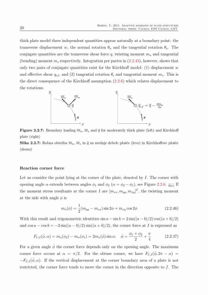
20Bohinc, U. 2011. Adaptive modeling of plate structures
Doctoral thesis. Cachan, ENS Cachan, LMT
thick plate model three independent quantities appear naturally at a boundary point: the
transverse displacement w, the normal rotation θn and the tangential rotation θs. The
conjugate quantities are the transverse shear force q, twisting moment mn and tangential
(bending) momentms respectively. Integration per partes in (2.2.43), however, shows that
only two pairs of conjugate quantities exist for the Kirchhoff model: (1) displacement w
and effective shear qef , and (2) tangential rotation θs and tangential moment ms. This is
the direct consequence of the Kirchhoff assumption (2.2.6) which relates displacement to
the rotations.
x
ymnms
q
s
x
yms
qef = q − ∂mn
∂s
s
Figure 2.2.7: Boundary loading mn, ms and q for moderately thick plate (left) and Kirchhoff
plate (right)
Slika 2.2.7: Robna obtezba mn, ms in q za srednje debele plosce (levo) in Kirchhoffove plosce
(desno)
Reaction corner force
Let us consider the point lying at the corner of the plate, denoted by I. The corner with
opening angle α extends between angles φ1 and φ2 (α = φ2 − φ1), see Figure 2.2.6. ¡¡¿¿ If
the moment stress resultants at the corner I are [mxx, myy, mxy]T , the twisting moment
at the side with angle φ is
mn(φ) =1
2(myy −mxx) sin 2φ+mxy cos 2φ (2.2.46)
With this result and trigonometric identities sin a− sin b = 2 sin((a− b)/2) cos((a+ b)/2)
and cos a− cos b = −2 sin((a− b)/2) sin((a+ b)/2), the corner force at I is expressed as
FC,I(φ, α) = mn(φ2)−mn(φ1) = 2mn(φ) sinα; φ =φ1 + φ2
2+π
4(2.2.47)
For a given angle φ the corner force depends only on the opening angle. The maximum
corner force occurs at α = π/2. For the obtuse corner, we have FC,I(φ, 2π − α) =
−FC,I(φ, α). If the vertical displacement at the corner boundary area of a plate is not
restricted, the corner force tends to move the corner in the direction opposite to f . The

Bohinc, U. 2011. Prilagodljivo modeliranje ploskovnih konstrukcij
Doktorska disertacija. Ljubljana, UL, Fakulteta za gradbenistvo in geodezijo, Konstrukcijska smer 21
reaction corner force is present if the displacement at corner boundary area is fixed. The
reaction corner force, however, does not appear if the edges meeting at the corner are free
or clamped, because the twisting moment mn on both sides of the corner point is zero.
Weak form of the problem
The weak form of the plate bending problem for the Kirchhoff model is
∫
Ω
m · β dΩ =
∫
Ω
u f dΩ +
∫
Γ
(qef u−ms∂u
∂n) ds (2.2.48)
The corner forces are omitted from the expression (2.2.48). The constitutive equation
and the kinematic equation are used point-wise. Therefore, the vector β is a function of
u only, since β = Lu and m = CBκ = CBLw, where κ = Lw. Left hand side of (2.2.48)
becomes a bilinear form of w and u
aK(w; u) =
∫
Ω
uLTCBLw dΩ (2.2.49)
while the right hand side is a linear functional of u only:
lK(u) =
∫
Ω
u f dΩ +
∫
Γ
(qef u−ms∂u
∂n) ds+
∑
i
FCiui (2.2.50)
The weak form of a thin plate Kirchhoff bending problem can be presented as
For given geometry, Dirichlet and Neumann boundary conditions and area loads, finddisplacement w ∈ V, such that
aK(w; u) = lK(u) ∀u ∈ V0 (2.2.51)
is satisfied for arbitrary test function u from the test space V0
The test space V consist of square integrable functions, which satisfy the boundary con-
dition of the problem, while the test space V0 consists of square integrable functions
which are zero at the part of the boundary where the Dirichlet boundary conditions are
prescribed.
Virtual work
The principle of virtual work can be regarded as the weak form of the equilibrium equa-
tions. That becomes clear if the test functions are denoted as u = δw and β = δκ where
δ stands for the variation. The variations δw and δ ∂w∂n
= ∂δw∂n
are zero at the boundary

22Bohinc, U. 2011. Adaptive modeling of plate structures
Doctoral thesis. Cachan, ENS Cachan, LMT
where the displacement w or rotation ∂w∂n
are defined, respectively. The virtual work of
internal forces for the thin plate is thus
δΠint =
∫
Ω
δκTm dΩ (2.2.52)
and the virtual work of external forces:
δΠext =
∫
Ω
δw f dΩ +
∫
Γ
(qef δw −ms∂δw
∂n) ds (2.2.53)
By using constitutive and kinematic equations m = CBκ = CBLw the virtual work
equation transforms into the weak problem. The equilibrium displacement w is such that
the virtual work of internal forces equals the virtual work of external forces for arbitrary
admissible virtual displacement δw, which conforms to the boundary conditions
δΠint = aK(w; δw) = δΠext = lK(δw) ∀δw ∈ V0 (2.2.54)
Boundary conditions
The part of the boundary, where displacement and its normal derivative is prescribed, is
called fixed boundary and the boundary conditions are expressed as
w = w; θs = −∂w∂n
= θs (2.2.55)
Since the test function u and its normal derivative are zero, at that parts nonzero contribu-
tion to (2.2.50) is only from the region of boundary where stress resultants are prescribed
(and displacements and its normal derivatives are not). The linear functional (2.2.50)
suggests that there are two independent loads on the boundary ΓN : moment ms and
shear force qef . The boundary conditions for the traction boundary are:
qef = qef ; ms = ms (2.2.56)
From (2.2.43) we notice that at free edges the shear force qef and the tangential moment
ms vanish. However, (2.2.44) shows that vanishing shear force qef = 0 does not necessarily
imply that the shear q at free edges also vanish. In fact the shear q and twisting moment
mn can both be nonzero at the free edges of the Kirchhoff plate. Another implication is
that the support forces are not identical to shear forces if the twisting moment exists.
Some common boundary conditions for the thin plate problem are listed in Table 2.1.
Notice, that the prescription of the displacement of the boundary implicitly defines also
the normal rotation. Since the Kirchhoff constraint along the boundary is γs =∂w∂s−θn = 0

Bohinc, U. 2011. Prilagodljivo modeliranje ploskovnih konstrukcij
Doktorska disertacija. Ljubljana, UL, Fakulteta za gradbenistvo in geodezijo, Konstrukcijska smer 23
Table 2.1: Boundary conditions for thin plates. ∗ θn = ∂w∂s is zero due to w = 0.
Tabela 2.1: Robni pogoji za tanke plosce. ∗ θn = ∂w∂s je nic zaradi w = 0.
Clamped (fixed): w = 0 θs = 0 θn = 0∗
Simply supported: w = 0 ms = 0 θn = 0∗
Free: qef = 0 ms = 0
the normal rotation is defined by θn = ∂w∂s. In the case of simply supported or clamped
boundary the constraint w = 0 implies also θn = 0. Therefore, with the Kirchhoff model
it is possible to model only hard simply supported boundary. The difference between the
hard and the soft simple support will be presented in the next chapter.
Principal directions of the moments
The twisting moment mn and the bending moment ms in a given direction at a point
(x, y) ∈ Ω are defined by (2.2.36). Let n in (2.2.36) be defined as n = [cosϕ, sinϕ]T .
From the condition mn = 0, one can compute angle ϕ at which the twisting moment
vanishes:
tan 2ϕ =2mxy
mxx −myy
(2.2.57)
The twisting moment has its extreme value at ϕ± π/2:
mmaxn =
√[mxx −myy
2
]2+m2
xy (2.2.58)
The maximum and minimum bending moment are:
mI,II =mxx +myy
2±mmax
n (2.2.59)
Singularities
An interesting implication of the Kirchhoff constraint occurs in the case of curved sim-
ply supported boundary, which is approximated by a polygonal boundary. The nor-
mal rotation at each corner point is defined twice - for each side a normal rotation
θn = ∂w∂s
= ∇w · s = 0 vanishes. Since the orientations of the sides meeting in cor-
ner point do not match, s1 6= s2, this is only possible when ∇w = 0 at the corner points
∇w · s1 = 0; ∇w · s2 = 0 ⇒ ∇w = 0 (2.2.60)

24Bohinc, U. 2011. Adaptive modeling of plate structures
Doctoral thesis. Cachan, ENS Cachan, LMT
αr ϕ
Figure 2.2.8: Definition of a polar coordinate system (r, ϕ) at the corner
Slika 2.2.8: Definicija polarnega koordinatnega sistema (r, ϕ) v vogalu
At corner points the plate is thus effectively clamped:
w =∂w
∂x=∂w
∂y= 0 (2.2.61)
The corner clamping is the source of singularity at the corner points of simply supported
polygonal boundary. The bending moments and shear forces may become singular.
The singular behavior of the solution in the vicinity of corner points has been studied
in several works for simply supported and other boundary conditions. For the illustration
of the approach we reexamine the case of a corner with opening angle α bounded by
two simply supported edges of a plate. This problem was first presented in [Morley,
1963]. A polar coordinate (r, ϕ) system is introduced (see Figure 2.2.8). The origin of the
coordinate system is in the corner point such that ϕ ∈ [−α/2,+α/2]. The biharmonic
equation in polar coordinates reads [Timoshenko Vojnovski-Kriger, 1959]
w = f/D; =∂2
∂r2+
1
r
∂
∂r+
1
r2∂2
∂ϕ2(2.2.62)
with the stress resultants defined as:
mr = −D((1− ν)∂2w
∂r2+ νw) (2.2.63)
mϕ = −D(w − (1− ν)∂2w
∂r2)
mrϕ = (1− ν)D(1
r
∂2w
∂r∂ϕ− 1
r2∂w
∂ϕ)
qr = −D ∂
∂rw; qϕ = −D1
r
∂
∂ϕw
The boundary conditions for a simply supported edge are:
w = 0; mϕ = 0 (2.2.64)

Bohinc, U. 2011. Prilagodljivo modeliranje ploskovnih konstrukcij
Doktorska disertacija. Ljubljana, UL, Fakulteta za gradbenistvo in geodezijo, Konstrukcijska smer 25
Since the displacement along the radial edge is constant (e.g. zero), we have ∂w∂r
= ∂2w∂r2
= 0
and the second condition mϕ = 0 is equivalent to w = 0. The general solution of
(2.2.62), (2.2.64) can be presented as a sum w = wp+wh of a particular solution wp and a
homogeneous solution wh, which is biharmonic. A particular solution wp, which satisfies
(2.2.62) and (2.2.64) at ϕ = ±α/2 is
wp =f r4
64D
(1− 4 cos(2ϕ)
3 cos(α)+
1
3
cos(4ϕ)
cos(2α)
)(2.2.65)
which can be checked by using it in (2.2.62) and (2.2.64). A special form of particular
solution is required for angles α=(π/4, π/2, 3π/4, 3π/2, 2π/2), when the cosine term in
the denominator is zero. The homogeneous solution is chosen as an infinite series of
eigenfunctions wh,m, i.e. wh =∑∞
m=1wh,m. Eigenfunctions which satisfy homogeneous
biharmonic equation, as well as the boundary conditions w = 0, w = 0 along the radial
edges at ϕ = ±α/2, arewh,m = (am + bmr
2)rλ cos(λϕ) (2.2.66)
where am and bm are constants and λ is chosen so that
cos(±λα/2) = 0 ⇒ λ = π/α(1 + 2m); m ≥ 0 (2.2.67)
For the displacement w and rotation ∂w∂r
to remain finite at r = 0 the condition λ ≥ 0
has been taken into account. The leading term in the expression for the displacement w
is of the form rλ cos(λϕ). From (2.2.63), we see that the leading term for the moments
mr and mϕ is rλ−2, while the leading term for the qr, qϕ and mrϕ is rλ−3. The singularity
occurs when the exponent is < 0. The singular behavior of (i) mr and mϕ is expected
when λ < 2 or α > π/2. Correspondingly, the singularity in (ii) qr, qϕ and mrϕ can
occur at angles α > π/3. At a given angle the strongest singularity occurs for the stress
components (ii) followed by one order weaker singularity in the components (i). The
strength of the singularity λ = π/α is inversely proportional to the opening angle α. The
angles α = π/4, π/2, 3π/4, 3π/2, 2π/2 are exceptions. In general, the leading term rλ in
this case is replaced by rλ(log r)p where p is an integer. In the neighborhood of these
exceptions the singular behavior is not continuous with respect to α. A list of critical
angles for Kirchhoff plates for different boundary conditions of intersecting edges is shown
in Table 2.2 (after [Melzer Rannacher, 1980]).
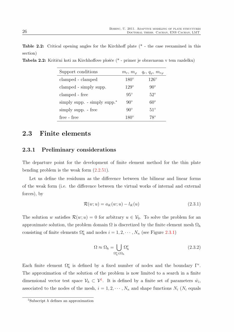
26Bohinc, U. 2011. Adaptive modeling of plate structures
Doctoral thesis. Cachan, ENS Cachan, LMT
Table 2.2: Critical opening angles for the Kirchhoff plate (* - the case reexamined in this
section)
Tabela 2.2: Kriticni koti za Kirchhoffove plosce (* - primer je obravnavan v tem razdelku)
Support conditions mr, mϕ qr, qϕ, mrϕ
clamped - clamped 180 126
clamped - simply supp. 129 90
clamped - free 95 52
simply supp. - simply supp.∗ 90 60
simply supp. - free 90 51
free - free 180 78
2.3 Finite elements
2.3.1 Preliminary considerations
The departure point for the development of finite element method for the thin plate
bending problem is the weak form (2.2.51).
Let us define the residuum as the difference between the bilinear and linear forms
of the weak form (i.e. the difference between the virtual works of internal and external
forces), by
R(w; u) = aK(w; u)− lK(u) (2.3.1)
The solution w satisfies R(w; u) = 0 for arbitrary u ∈ V0. To solve the problem for an
approximate solution, the problem domain Ω is discretized by the finite element mesh Ωh
consisting of finite elements Ωeh and nodes i = 1, 2, · · · , Nn (see Figure 2.3.1)
Ω ≈ Ωh =⋃
Ωeh∈Ωh
Ωeh (2.3.2)
Each finite element Ωeh is defined by a fixed number of nodes and the boundary Γe.
The approximation of the solution of the problem is now limited to a search in a finite
dimensional vector test space Vh ⊂ V1. It is defined by a finite set of parameters wi,
associated to the nodes of the mesh, i = 1, 2, · · · , Nn and shape functions Ni (Ni equals
1Subscript h defines an approximation

Bohinc, U. 2011. Prilagodljivo modeliranje ploskovnih konstrukcij
Doktorska disertacija. Ljubljana, UL, Fakulteta za gradbenistvo in geodezijo, Konstrukcijska smer 27
1 at node i, and 0 at all other nodes)2
wh =Nn∑
i
Niwi (2.3.3)
After Bubnov and Galerkin, the optimal approximation of the solution is the one for
which the residuum is zero only for the arbitrary test function uh from the test space V0,h
R(wh; uh) = 0 ∀uh ∈ V0,h (2.3.4)
The test space V0,h is spanned over the shape functions Ni. An arbitrary test function
uh is a linear combination of shape functions: uh =∑
iNiui. The residuum for arbitrary
test function uh vanishes, if it vanishes for each shape function Ni
R(wh, Ni) = 0 or∑
j
aK(Nj , Ni) wj = lK(Ni) ∀Ni (2.3.5)
In the matrix form
Ku = f (2.3.6)
whereK = [Kij] = [aK(Ni, Nj)], u = [w1, w2, · · · , wNn]T and f = [lK(N1), lK(N2), · · · , lK(NNn
)]T .
The linear system (2.3.6) is finally solved for the unknown parameters u.
The approximate solution can be also searched from the spirit of the principle of virtual
work. The solution wh =∑
iNiwi must be such that the virtual work of internal forces
δΠint equals the virtual work of external forces δΠext for arbitrary virtual displacement
δwh =∑
iNiδwi, member of the test space V0,h
δΠint = δΠext ∀δwh ∈ V0,h (2.3.7)
δΠint = aK(wh; δwh); δΠext = lK(δwh)
From wh =∑
iNiwi and δwh =∑
iNiδwi we have
δΠint = aK(wh;∑
i
Niδwi) =∑
i
aK(wh;Ni)δwi =∑
i
∑
j
wjaK(Nj, Ni)δwi
where the linearity of bilinear form aK was exploited. Using the matrix notation we have
δΠint = δuTKu; K = [Kij ] = aK(Nj, Ni); δu = [δw1, δw2, · · · , δwn]T (2.3.8)
2For the sake of compactness the shape functions Ni are here defined over the whole domain Ωh

28Bohinc, U. 2011. Adaptive modeling of plate structures
Doctoral thesis. Cachan, ENS Cachan, LMT
δΠext = lK(δwh) =∑
i
δwilK(Ni) = δuTf ; f = [fi] = [lK(Ni)] (2.3.9)
Inserting the relations (2.3.8) and (2.3.9) into (2.3.7) we obtain
δuT (Ku− f ) = 0 (2.3.10)
Due to the fact that the variations δwi are arbitrary and independent, the equation
(2.3.10) is fulfilled only when Ku− f = 0 holds. This is equivalent to (2.3.6).
Ω Ωh
Γ Γh
Ωeh
i
Pi
Figure 2.3.1: Problem domain Ω and its boundary Γ (left), finite element discretization Ωeh,
Ωh and patch of elements ΩPi
h around node i (right)Slika 2.3.1: Obmocje Ω in njegov rob Γ (levo), diskretizacija s koncnimi elementi Ωe
h, Ωh in
krpa elementov ΩPi
h okoli vozlisca i (desno)
Shape functions
The shape function Ni takes unit value at node i and is zero at all other nodes of the finite
element mesh. The shape function Ni is nonzero only on a finite domain ΩPi
h . Hence, the
adjective ‘finite‘ in the name of the method.
Let m denote the variational index of the variational functional (the highest deriva-
tive present in the functional) that is to be solved by the finite element method. A basic
requirement for the convergence of approximate solution is that the shape functions sat-
isfy the completeness condition: the element shape functions must exactly represent all
polynomial terms of order ≤ m in the Cartesian coordinates. In the case of (2.2.51),
the variational index is m = 2, therefore the interpolation on Ωeh should be able to rep-
resent any field, which is a linear or quadratic polynomial in x and y; in particular, a
constant value. Constant and linear polynomials represent rigid body motions, whereas
quadratic polynomials represent constant curvature modes. The C0 continuity requires
that the shape functions are continuous across the element edges. The shape functions

Bohinc, U. 2011. Prilagodljivo modeliranje ploskovnih konstrukcij
Doktorska disertacija. Ljubljana, UL, Fakulteta za gradbenistvo in geodezijo, Konstrukcijska smer 29
are continuous only if the displacement over any side of the element is defined only by
DOFs on that side. The second derivatives in (2.2.51) indicate that the shape functions
must satisfy not only C0 but also C1 continuity - continuity of the slopes of the shape
functions. This can only be achieved if the shape functions are C0 continuous and the
normal slope ∂w∂n
over any edge of the element is completely defined only by the DOFs on
that edge. The elements based on C1 continuous shape functions are often referred to as
conforming or compatible.
While obtaining C0 continuity is relatively simple, this is certainly not the case with
C1 continuity. It was proven in ([Zienkiewicz Taylor, 2000], [Felippa, 2009]) that, when
only w and its slopes are prescribed at the corner nodes, it is impossible to specify simple
polynomial expressions for shape functions, which ensure the full compatibility.
2.3.2 An overview of thin plate elements
Among the first successful conforming plate elements was the rectangular element with 16
DOFs (w, w,x,w,y and w,xy at each node) developed by [Bogner et al., 1966]. The element
uses Hermitian interpolation functions with bi-cubic shape functions. The triangular
elements offer more flexibility in the design of the conforming elements that the rectangular
ones. It was shown in [Felippa, 2009] that a complete fifth order polynomial is the first
which satisfy the C1 continuity requirements. From the Pascal’s triangle it follows that
the complete quintic polynomial contains 21 terms. Conforming triangular plate element
with 21 DOFs was independently developed by several authors ([Argyris et al., 1968]
et al., [Bell, 1969], [Bosshard, 1968], [Visser, 1968]). Conforming quadrilateral elements
can be produced from the conforming triangular elements. If the combined element has
an additional internal degrees of freedom they are eliminated by static condensation. A
direct derivation of conforming quadrilateral element is also possible. The derivation was
first proposed by [Sander, 1964] and [De Veubeke, 1968].
Although the conforming plate elements exhibit excellent accuracy and performance
they have some important drawbacks. The C1 continuity presents a difficulty when dis-
continuous variation of material properties occurs. It is also difficult to impose the right
boundary conditions since ’nodal forces’ as energy conjugates to chosen degrees of freedom
can no longer be interpreted intuitively.
It is relatively simple to obtain shape functions, which respect C0 continuity but violate
the slope continuity between the elements. They can still be used to build plate elements.
It is namely possible to found the convergence of such elements if only they pass the

30Bohinc, U. 2011. Adaptive modeling of plate structures
Doctoral thesis. Cachan, ENS Cachan, LMT
”patch test” [Zienkiewicz Taylor, 2000]. They are referred to as non-conforming and can
in many cases perform even better than the conforming ones. Additional conditions for
the shape functions follow from the patch test. They are formulated for each straight side
of the element Γ: ∫
Γ
∆(∂w
∂n)ds = 0;
∫
Γ
∆(∂w
∂s)ds = 0. (2.3.11)
where ∆ denotes the mismatch along the side of neighboring elements. Notice that, if the
function w and its first derivatives are defined at the corner nodes, the satisfaction of the
second condition in (2.3.11) is always ensured.
An early attempt to build a conforming rectangular element lead to the formulation
of the first successful non-conforming quadrilateral plate bending element proposed by
[Adini Clough, 1960]. The element has 12 DOFS and it satisfies completeness as well
as transverse deflection continuity but normal slope continuity is maintained only at four
corner points. One of the first successful non-conforming triangular plate elements is
that presented by [Bazeley et al., 1965]. The element has nine DOFs. Since full cubic
expansion contains 10 terms, one DOF is eliminated in such a way that the completeness
is maintained. Although the element satisfies constant curvature criterion it does not pass
the patch test for arbitrary mesh configurations. Despite the shortcomings the element
became quite popular in practical applications.
A rather successful approach involves a direct interpolation of displacement w and
rotation θ. Due to the independent interpolations the continuity requirement is only C0
for both unknowns w and θ. The interpolations are constructed such that the Kirchhoff
constrain is satisfied only in certain discrete collocation points. Hence the name discrete
Kirchhoff - DK elements. It is possible to impose the Kirchhoff constraint along the sides
of the element resulting in superior performance. The most successful elements of this
type are discrete Kirchhoff triangle (DKT) and discrete Kirchhoff quadrilateral (DKQ)
([Dhatt, 1970], [Batoz et al., 1980] and [Batoz, 1982]). Many finite element analyses of a
plate bending problem are done with DK plate elements. They are widely accepted due
to their efficiency and ease of use. One of the reasons for their popularity is also the fact
that they employ only displacement and rotations as the nodal degrees of freedom.
2.3.3 Natural coordinate systems
We have thought of shape function Ni in section 2.3.1 as of a function defined over ΩPi
h .
In practice, the shape functions are defined over a finite element Ωeh.

Bohinc, U. 2011. Prilagodljivo modeliranje ploskovnih konstrukcij
Doktorska disertacija. Ljubljana, UL, Fakulteta za gradbenistvo in geodezijo, Konstrukcijska smer 31
The description of the element shape functions in the Cartesian coordinates (x, y) is
not very convenient. We therefore seek for coordinates ξi, i = 1, 2 such that the location
of a point P (x, y) inside an element defined by nodes (xi, yi), i = (1, 2, 3)(triangle) or i =
(1, 2, 3, 4)(quadrilateral) would be described in a ”natural” way; i.e. as x =∑
iNi(ξk)xi
where Ni is now an element shape function, defined by ξi over Ωeh. The coordinate system
which emerges naturally is therefore called a natural coordinate system.
Quadrilateral geometry
The natural coordinate system for the element with quadrilateral geometry is shown in
Figure 2.3.2 (ξ1 = ξ, ξ2 = η). The location of a point P (x, y) is given as
x
y4
1
2
3
Ωeh
P (x, y)
1 2
4 3
ξ
η
-1 0 +1
-1
+1Ω
Figure 2.3.2: Bi-unit element Ω in coordinate system (ξ,η)
Slika 2.3.2: Enotski element Ω v koordinatnem sistemu (ξ,η)
x = N1x1 +N2x2 +N3x3 +N4x4; y = N1y1 +N2y2 +N3y3 +N4y4 (2.3.12)
or in matrix form
[xy
]=
[x1 x2 x3 x4y1 y2 y3 y4
]
N1
N2
N3
N4
(2.3.13)
where Ni are bilinear Lagrangian functions; defined over Ω as:
N1 = (1− ξ)(1− η)/4; N2 = (1 + ξ)(1− η)/4 (2.3.14)
N3 = (1 + ξ)(1 + η)/4; N4 = (1− ξ)(1 + η)/4

32Bohinc, U. 2011. Adaptive modeling of plate structures
Doctoral thesis. Cachan, ENS Cachan, LMT
The differentials of (x, y) are related to those of (ξ, η) and vice versa by:
[dxdy
]=
[∂x∂ξ
∂x∂η
∂y∂ξ
∂y∂η
]
︸ ︷︷ ︸J
[dξdη
];
[dξdη
]= J−1
[dxdy
](2.3.15)
The Jacobian of the transformation is denoted by J and is computed from (2.3.15), (2.3.12)
and (2.3.14):
J =∑
i
[∂Ni
∂ξxi
∂Ni
∂ηxi
∂Ni
∂ξyi
∂Ni
∂ηyi
]=
[x1 x2 x3 x4y1 y2 y3 y4
]
∂N1
∂ξ∂N1
∂η∂N2
∂ξ∂N2
∂η∂N3
∂ξ∂N3
∂η∂N4
∂ξ∂N4
∂η
(2.3.16)
The derivatives of a function f with respect to the global coordinates (x, y) are related
to the derivatives of f in the natural coordinate system by
[ ∂f∂x∂f∂y
]=
[ ∂ξ∂x
∂η∂x
∂ξ∂y
∂η∂y
][ ∂f∂ξ∂f∂η
]= J−T
[∂f∂ξ∂f∂η
](2.3.17)
The integration over the element domain is performed in the natural coordinates over the
unit element Ω = (ξ, η), ξ ∈ [−1,+1], η ∈ [−1,+1]:
∫
Ωeh
fdxdy =
∫
Ω
f(ξ, η) detJ dξdη (2.3.18)
The expression for the determinant of Jacobian can be simplified into:
detJ = (AΩeh+ d1ξ + d2η)/4 (2.3.19)
d1 = ((x4 − x3)(y2 − y1)− (x2 − x1)(y4 − y3))/2
d2 = ((x3 − x2)(y4 − y1)− (x4 − x1)(y3 − y2))/2
The area of the element is denoted as AΩehand the parameters d1 and d2 define the
distortion of the quadrilateral element. Distortion vanishes if the quadrilateral element is
parallelogram. In that case detJ is constant. Figure 2.3.3 shows the quadrilateral element
with the coordinate lines of the natural coordinate system. Alternate shading between
the coordinate lines is used to illustrate the variation of values of detJ.
Triangular geometry
The coordinates used for the triangular elements are often called area, natural or even
barycentric coordinates. The coordinates are denoted by (ξ1 = ζ1, ξ2 = ζ2, ξ3 = ζ3) with ζ3

Bohinc, U. 2011. Prilagodljivo modeliranje ploskovnih konstrukcij
Doktorska disertacija. Ljubljana, UL, Fakulteta za gradbenistvo in geodezijo, Konstrukcijska smer 33
Figure 2.3.3: Quadrilateral element with the alternate shading between the coordinate linesof the quadrilateral natural coordinate systemSlika 2.3.3: Stirikotni element z izmenicnim sencenjem med koordinatnimi crtami naravnegakoordinatnega sistema
being function of ζ1 and ζ2. The coordinate line ζi = const. is parallel to the side opposite
to node i. The term area coordinates originates from the definition. Let us consider a
point p inside the triangle defined by the nodes i, j, k. The triangle coordinate of the point
is ζi = Apjk/Aijk (see Figure 2.3.4). Area of the triangle ijk is denoted by Aijk, while Apjk
is the area of the triangle defined by the nodes p, j and k. Since Aijk = Apij+Apjk+Apki
the sum of the coordinates equals to unity
Figure 2.3.4: Triangular (area) coordinatesSlika 2.3.4: Trikotniske koordinate
34Bohinc, U. 2011. Adaptive modeling of plate structures
Doctoral thesis. Cachan, ENS Cachan, LMT
1 = ζ1 + ζ2 + ζ3; x = ζ1x1 + ζ2x2 + ζ3x3; y = ζ1y1 + ζ2y2 + ζ3y3 (2.3.20)
or in matrix form
1xy
=
1 1 1x1 x2 x3y1 y2 y3
ζ1ζ2ζ3
(2.3.21)
By inverting this relation, we get:ζ1ζ2ζ3
=
1
2AΩeh
x2 y3 − x3 y2 +y2 − y3 −x2 + x3x3 y1 − x1 y3 +y3 − y1 −x3 + x1x1 y2 − x2 y1 +y1 − y2 −x1 + x2
1xy
(2.3.22)
where (xi, yi) are the coordinates of the nodes of the triangle and AΩehis its area. The
Jacobian of the triangular coordinate transformation is
J =
1 1 1x1 x2 x3y1 y2 y3
(2.3.23)
The detJ is twice the area of the triangle: detJ = 2AΩeh. The integral over the element
domain is performed in the natural coordinates over the unit element Ω:∫
Ωeh
fdxdy =1
2
∫
Ω
f(ζ1, ζ2, ζ3) detJ dΩ = AΩeh
∫
Ω
f(ζ1, ζ2, ζ3) dΩ (2.3.24)
Since the unit element is a triangle, we have
∫
Ω
f(ζ1, ζ2, ζ3) dΩ =
∫ 1
0
dζ1
∫ 1−ζ1
0
f(ζ1, ζ2, 1− ζ1 − ζ2) dζ2
Derivatives with respect to global coordinates (x, y) are related to the derivatives with
respect to the triangular coordinates (ζ1, ζ2, ζ3) via
[ ∂f∂x∂f∂y
]=
[ ∂ζ1∂x
∂ζ2∂x
∂ζ3∂x
∂ζ1∂y
∂ζ2∂y
∂ζ3∂y
]
∂f∂ζ1∂f∂ζ2∂f∂ζ3
(2.3.25)
From (2.3.22) we have
[ ∂f∂x∂f∂y
]=
1
2AΩeh
[y2 − y3 y3 − y1 y1 − y2x3 − x2 x1 − x3 x2 − x1
]
∂f∂ζ1∂f∂ζ2∂f∂ζ3
(2.3.26)
and from (2.3.21)
∂f∂ζ1∂f∂ζ2∂f∂ζ3
=
x1 y1x2 y2x3 y3
[ ∂f
∂x∂f∂y
](2.3.27)
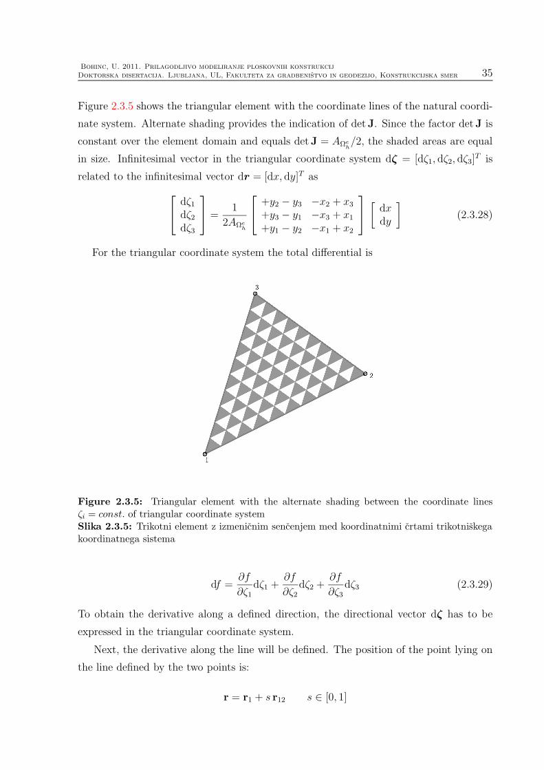
Bohinc, U. 2011. Prilagodljivo modeliranje ploskovnih konstrukcij
Doktorska disertacija. Ljubljana, UL, Fakulteta za gradbenistvo in geodezijo, Konstrukcijska smer 35
Figure 2.3.5 shows the triangular element with the coordinate lines of the natural coordi-
nate system. Alternate shading provides the indication of detJ. Since the factor detJ is
constant over the element domain and equals detJ = AΩeh/2, the shaded areas are equal
in size. Infinitesimal vector in the triangular coordinate system dζ = [dζ1, dζ2, dζ3]T is
related to the infinitesimal vector dr = [dx, dy]T as
dζ1dζ2dζ3
=
1
2AΩeh
+y2 − y3 −x2 + x3+y3 − y1 −x3 + x1+y1 − y2 −x1 + x2
[dxdy
](2.3.28)
For the triangular coordinate system the total differential is
Figure 2.3.5: Triangular element with the alternate shading between the coordinate linesζi = const. of triangular coordinate systemSlika 2.3.5: Trikotni element z izmenicnim sencenjem med koordinatnimi crtami trikotniskegakoordinatnega sistema
df =∂f
∂ζ1dζ1 +
∂f
∂ζ2dζ2 +
∂f
∂ζ3dζ3 (2.3.29)
To obtain the derivative along a defined direction, the directional vector dζ has to be
expressed in the triangular coordinate system.
Next, the derivative along the line will be defined. The position of the point lying on
the line defined by the two points is:
r = r1 + s r12 s ∈ [0, 1]

36Bohinc, U. 2011. Adaptive modeling of plate structures
Doctoral thesis. Cachan, ENS Cachan, LMT
where r12 = r2 − r1. Inserting dr = [dx, dy]T = ds[(x2 − x1), (y2 − y1)]T into (2.3.28), we
obtain
dζ = [dζ1, dζ2, dζ3]T = ds[−1,+1, 0].
The derivative along the direction r12 with respect to the parameter s is given by (2.3.29)
∂f
∂s= (
∂f
∂ζ2− ∂f
∂ζ1) ≡ f,12 (2.3.30)
The definition of the second derivative along the line is straightforward
∂2f
∂s2=
∂
∂s(∂f
∂ζ2− ∂f
∂ζ1)) = (
∂2f
∂ζ22− 2
∂f
∂ζ1
∂f
∂ζ2+∂2f
∂ζ21) ≡ f,122 (2.3.31)
To determine the derivative with respect to the normal to the side of the triangle, one
has to follow similar steps. First we parameterize the perpendicular line to a side (in this
case side 1-2) going through the side middle point:
r =1
2(r1 + r2) + 2 ds h3n12 = r12 + 2ds h3n12 (2.3.32)
where n12 is a normal vector to the side 1-2 with length l12, h3 is height of point 3 and
r12 =12(r1 + r2). The differential vector dr = 2ds h3n12 is in the global basis
dr =
[dxdy
]= 2ds h3
[+y2 − y1−x2 + x1
]/l12 (2.3.33)
and can be written in the triangular basis using (2.3.28):
dζ =
dζ1dζ2dζ3
=
2h32AΩe
h
−(y3 − y2) +(x3 − x2)+(y3 − y1) −(x3 − x1)−(y2 − y1) +(x2 − x1)
[
+y2 − y1−x2 + x1
]/ l12
We further notice that AΩeh= h3 l12/2, introduce the notation xij = xj − xi, and rewrite
the upper expression as
dζ =
dζ1dζ2dζ3
=
2
l212
−y23 y12 − x23 x12+y13 y12 + x13 x12
−l212
=
+1− 2 r12 · (r3 − r12)/l212
+1 + 2 r12 · (r3 − r12)/l212
−2
(2.3.34)
We introduce the parameter µ12 = 2r12 · (r3 − r12)/l212 = 2e1/l12, which has a meaning
of normalized eccentricity of node 3 with respect to the symmetry line of edge 1-2 (see
Figure 2.3.6). Finally, we have
dζ1 = (1− µ12) ds; dζ2 = (1 + µ12) ds; dζ3 = 2ds (2.3.35)
and the derivative normal to the edge 1-2
∂f
∂n= 2
∂f
∂ζ3− (
∂f
∂ζ1+∂f
∂ζ2) + µ12 (
∂f
∂ζ2− ∂f
∂ζ1) = f,n (2.3.36)

Bohinc, U. 2011. Prilagodljivo modeliranje ploskovnih konstrukcij
Doktorska disertacija. Ljubljana, UL, Fakulteta za gradbenistvo in geodezijo, Konstrukcijska smer 37
Figure 2.3.6: To the definition of eccentricity parameter µ12 = 2e1/l12Slika 2.3.6: K definiciji parametra ekscentricnosti µ12 = 2e1/l12
2.3.4 Conforming triangular element
The derivation of the element presented below follows the work of [Argyris et al., 1968].
Here, only the outline of the derivation procedure will be presented. The element will be
called TUBA6 or Argyris element in what follows.
The displacement field is interpolated with complete 5th order polynomial in natural
(area) coordinates (ζ1, ζ2, ζ3). Namely, the complete quintic polynomial, defined with
21 parameters, is the lowest discrete approximation, which satisfies C1 continuity across
element boundaries [Zienkiewicz Taylor, 2000], [Argyris et al., 1968]. Hence, the discrete
approximation of the displacement field can be written as:
wh = ωT p (2.3.37)
where p = [p1, p2, · · · , p21]T denotes a vector of nodal interpolation parameters and ω the
set of shape functions. The latter contains 21 polynomials and can be written as:
ω = [ζ51 , ζ52 , ζ
53 ,
ζ1ζ42 , ζ2ζ
43 , ζ3ζ
41 , ζ2ζ
41 , ζ3ζ
42 , ζ1ζ
43 ,
ζ31ζ22 , ζ
32ζ
23 , ζ
33ζ
21 , ζ
32ζ
21 , ζ
33ζ
22 , ζ
31ζ
23 ,
ζ31ζ2ζ3, ζ1ζ32ζ3, ζ1ζ2ζ
33 , ζ
21ζ
22ζ3, ζ
21ζ2ζ
23 , ζ1ζ
22ζ
23 ]
T
The element nodal interpolation parameters pertain to 3 vertex nodes and 3 mid-side
nodes. Each vertex node has 6 degrees of freedom: displacement, its first derivatives,

38Bohinc, U. 2011. Adaptive modeling of plate structures
Doctoral thesis. Cachan, ENS Cachan, LMT
1
2
3
w1
w1,x, w1,y
w1,xx, w1,xy, w1,yy
w,n23
Figure 2.3.7: Triangular Argyris plate element - ARGY
Slika 2.3.7: Trikotni Argyrisov koncni element za plosce - ARGY
and its second derivatives with respect to x and y. The mid-side nodes contain the first
derivative in the direction of the exterior normal. The complete set of global degrees of
freedom can be written as:
w = [w1, w2, w3, w1,x, w1,y, w2,x, w2,y, w3,x, w3,y,
w1,xx, w1,xy, w1,yy, w2,xx, w2,xy, w2,yy, w3,xx, w3,xy, w3,yy,
w,n12, w,n23, w,n31 ]T
To establish the relation between p and w, all the derivatives are computed at the nodes.
As an intermediate step, we introduce an additional set of degrees of freedom wρ, where
the derivatives are formed with respect to natural (area) coordinates:
wρ = [ w1, w2, w3, w1,12, w1,31, w2,23, w2,12, w3,31, w3,23,
w1,122 , w1,312 , w1,232 , w2,122 , w2,312 , w2,232 , w3,122, w3,312 , w3,232 ,
w,n12 , w,n23, w,n31]T
The relation between p and wρ is defined by the system of equations which are obtained
by using results in (2.3.30), (2.3.31) and (2.3.36) at the nodes of the element. At node 1

Bohinc, U. 2011. Prilagodljivo modeliranje ploskovnih konstrukcij
Doktorska disertacija. Ljubljana, UL, Fakulteta za gradbenistvo in geodezijo, Konstrukcijska smer 39
(ζ1 = 1, ζ2 = 0, ζ3 = 0) we thus have:
w1 = p1 (2.3.38)
w1,12 = −5p1 + p4
w1,31 = +5p1 − p5
w1,122 = 20p1 − 10p1p4 + 2p10
w1,312 = 20p1 − 10p1p5 + 2p11
w1,232 = −2p4p5 + 2p10 + 2p11
and at the midside node on edge 1− 2 (ζ1 = 1/2, ζ2 = 1/2, ζ3 = 0) we have
w,n12 =(−5(1 + µ12)p1 + 5(−1 + µ12)p2 − (5 + 3µ12)p4 (2.3.39)
+ 2p5 + 2p6 − (5− 3µ12)p7 − (5 + µ12)p10
− (5− µ12)p13 + 2p16 + 2p17 + 2p19)/16
A linear system can be formed by writing down the equations (2.3.38) and (2.3.39) for all
the nodes:
wρ = A−1p (2.3.40)
where the matrix of the linear system is denoted as A−1.
From (2.3.30) we have:w,12w,23w,31
=
x12 y12x23 y23x31 y31
[w,xw,y
](2.3.41)
and from (2.3.31) we getw,122w,312w,232
=
x212 y212 −x12y12x231 y231 −x31y31x223 y223 −x23y23
︸ ︷︷ ︸T−1
w,xxw,yy2w,xy
(2.3.42)
This relations enable to define the transformation between w and wρ, which can be written
in matrix notation as wρ = XT w, where XT is matrix of the linear transformation. We
insert this result in (2.3.40) and obtain
p = Xw; X = AXT (2.3.43)
The discrete approximation of curvature vector κh is the second derivative of the
displacement field wh = ωTXw according to (2.2.8):
κh =
wh,xxwh,yy2wh,xy
(2.3.44)

40Bohinc, U. 2011. Adaptive modeling of plate structures
Doctoral thesis. Cachan, ENS Cachan, LMT
Computing further the inverse of the relation (2.3.42), we obtain:
κh = Tκh,ρ; κh,ρ = [wh,122 , wh,232 , wh,312 ]T = ωT
,ρw (2.3.45)
where ω,ρ = [ω,122,ω,232 ,ω,312 ]T .
Stiffness matrix
The element stiffness matrix is obtained from the bilinear form defined for a single element
aK,e(wh; uh) =
∫
Ωeh
κTh (uh)mh(wh) dΩ =
∫
Ωeh
κTh (uh)CB κh(wh) dΩ
=
∫
Ωeh
κTh,ρ(uh)T
T CB Tκh,ρ(wh) dΩ (2.3.46)
where the interpolation of the displacement is wh = ωTXw and of the test function
uh = ωTXu where u is vector of test function nodal parameters in cartesian coordinates.
The product G = TT CB T is constant in the case of homogeneous material. In that case
it remains only to evaluate the integral
∫
Ωeh
κTh,ρ(uh)κh,ρ(wh) dΩ = uT
(∫
Ωeh
ω,ρTω,ρ dΩ
)u = uTS w (2.3.47)
where S is obtained by analytic integration with the use of:
1
Ω
∫
Ω
ζp1ζq2ζ
r3 dΩ =
2! p! q! r!
(2 + p+ q + r)!(2.3.48)
The expression (2.3.46) can be put in a familiar matrix form
aK,e(wh; uh) = uT
[∑
i,j
GijSij
]w = uTKw. (2.3.49)
where K = [Kij ] = [∑
i,j GijSij ] is the stiffness matrix of the element.
Load vector
The equivalent load vector is computed from the virtual work of external forces (pressure
load f and boundary tractions qef ,ms)
lK,e(uh) =
∫
Ωeh
uh f dΩ +
∫
Γe
(uh qef −ms∂uh∂n
) ds (2.3.50)
= uTXT
(∫
Ωeh
ω f dΩ +
∫
Γe
(ω qef −ms∂ω
∂n) ds
)

Bohinc, U. 2011. Prilagodljivo modeliranje ploskovnih konstrukcij
Doktorska disertacija. Ljubljana, UL, Fakulteta za gradbenistvo in geodezijo, Konstrukcijska smer 41
By using (2.3.43) the nodal load vector f is finally written as:
f = XT
(∫
Ωeh
ω f dΩ +
∫
Γe
(ω qef −ms∂ω
∂n)
)(2.3.51)
The derivatives ∂ω∂n
are evaluated with the use of (2.3.36). The integrals in (2.3.51) can
be obtained in a closed form with the aid of the formula (2.3.48).
2.3.5 Discrete Kirchhoff elements
The motivation for the Discrete Kirchhoff (DK) plate elements is based on the observation
that it is quite challenging to construct a conforming approximation of the plate displace-
ment field. Since the Kirchhoff constraint of zero shear strains is very difficult to satisfy
at every point of the domain, a compromise is made: the constraint γ = ∇w − θ = 0 is
relaxed and is satisfied only at chosen points and directions. Relaxation of the Kirch-
hoff constraint implies that the discretization of displacement wh and rotations θh are no
longer tied together but are rather independent. They are related only along the sides of
the element. Otherwise independent interpolations for displacement wh and rotations θh
are constructed such that the shear strain γh along the element boundary (in the direction
s) vanishes
γh · s =∂wh
∂s− n · θh = 0 (2.3.52)
Edge interpolation equals beam element interpolation
To illustrate the idea, let us consider a discretization of the Euler Bernoulli beam, see
Figure 2.3.9. Two independent interpolations of displacement wh and rotation θh are set:
wh = w1N1 + w2N2 + w3N3 + w4N4 (2.3.53)
θh = θ1N1 + θ2N2 + θ3N3 (2.3.54)
where the hierarchic shape functions are (see Figure 2.3.8):
N1 = (1− ξ)/2; N2 = (1 + ξ)/2 ξ ∈ [−1,+1] (2.3.55)
N3 = (1− ξ2); N4 = ξ(1− ξ2)
Due to the requirement for the C1 continuity of the displacement, the order of the
interpolation is cubic. Only nodal displacements w1, w2 and rotations θ1, θ2 are acceptable

42Bohinc, U. 2011. Adaptive modeling of plate structures
Doctoral thesis. Cachan, ENS Cachan, LMT
Figure 2.3.8: Hierarchical shape functionsSlika 2.3.8: Hierarhicne interpolacijske funkcije
ξ
L
1 2
θ1 θ2w1 w2
z
x
x = L2(1 + ξ)
Figure 2.3.9: Euler-Bernoulli beam element
Slika 2.3.9: Koncni element za nosilec po Euler-Bernoullijevi teoriji
nodal degrees of freedom. Other parameters w3, w4, θ3 are thus eliminated by enforcing
the constraint of vanishing transverse shear strain γh = ∂wh
∂x− θh = 0. One gets from the
latter equation and (2.3.53), (2.3.54)
w3 = +L
8(θ1 − θ2); w4 =
L
4(w2 − w1
L− 1
2(θ1 + θ2)); θ3 =
6
Lw4 (2.3.56)
Using (2.3.56), the interpolations (2.3.53) and (2.3.54) become:
wh = w1H1 + w2H2 + θ1H3 + θ2H4 (2.3.57)
θh =1
4θ1(3ξ2 − 2ξ − 1
)+
1
4θ2(3ξ2 + 2ξ − 1
)+
3(w2 − w1)
2L(1− ξ2)
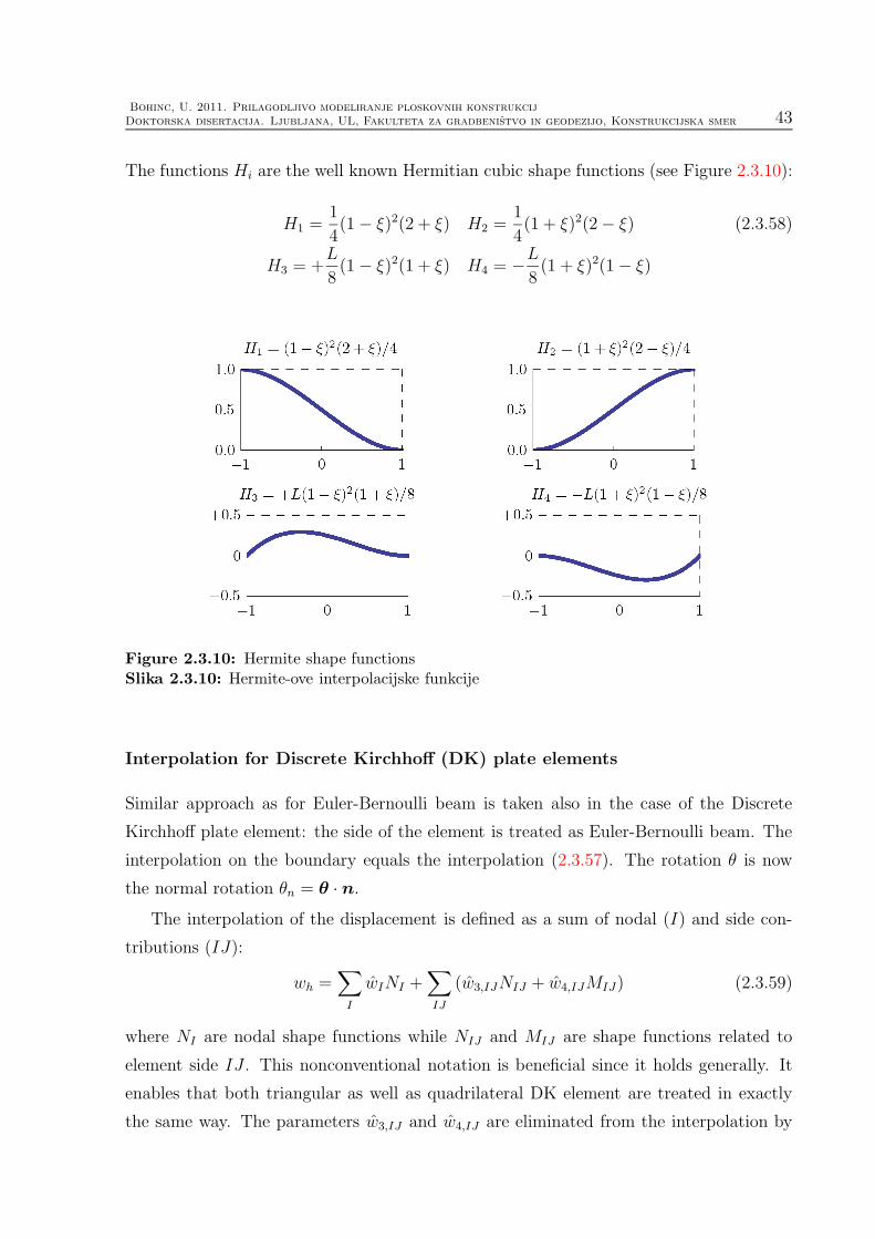
Bohinc, U. 2011. Prilagodljivo modeliranje ploskovnih konstrukcij
Doktorska disertacija. Ljubljana, UL, Fakulteta za gradbenistvo in geodezijo, Konstrukcijska smer 43
The functions Hi are the well known Hermitian cubic shape functions (see Figure 2.3.10):
H1 =1
4(1− ξ)2(2 + ξ) H2 =
1
4(1 + ξ)2(2− ξ) (2.3.58)
H3 = +L
8(1− ξ)2(1 + ξ) H4 = −L
8(1 + ξ)2(1− ξ)
Figure 2.3.10: Hermite shape functionsSlika 2.3.10: Hermite-ove interpolacijske funkcije
Interpolation for Discrete Kirchhoff (DK) plate elements
Similar approach as for Euler-Bernoulli beam is taken also in the case of the Discrete
Kirchhoff plate element: the side of the element is treated as Euler-Bernoulli beam. The
interpolation on the boundary equals the interpolation (2.3.57). The rotation θ is now
the normal rotation θn = θ · n.The interpolation of the displacement is defined as a sum of nodal (I) and side con-
tributions (IJ):
wh =∑
I
wINI +∑
IJ
(w3,IJNIJ + w4,IJMIJ) (2.3.59)
where NI are nodal shape functions while NIJ and MIJ are shape functions related to
element side IJ . This nonconventional notation is beneficial since it holds generally. It
enables that both triangular as well as quadrilateral DK element are treated in exactly
the same way. The parameters w3,IJ and w4,IJ are eliminated from the interpolation by

44Bohinc, U. 2011. Adaptive modeling of plate structures
Doctoral thesis. Cachan, ENS Cachan, LMT
enforcing zero transverse shear strain along the side IJ . It turns out that
w3,IJ =LIJ
8nIJ · (θI − θJ); (2.3.60)
w4,IJ =LIJ
4(wJ − wI
LIJ
− 1
2nIJ · (θI + θJ))
where θI = [θxI , θyI ] and LIJ is length of side between nodes I and J , and nIJ is normal
to the side between nodes I and J . Note the similarity between (2.3.60) and (2.3.56).
The interpolation of the rotation is defined as
θh =
[θx,hθy,h
]=
3∑
I=1
θINI +∑
IJ
θ3,IJnIJNIJ (2.3.61)
where, due to zero transverse shear strain along the side IJ (2.3.56)
θ3,IJ =6
Lw4,IJ (2.3.62)
The above interpolation leads to an element with only vertex nodes with degrees of free-
dom denoted by wI = [wI , θxI , θyI ]T . The interpolations (2.3.59) and (2.3.61) can also be
expressed as:
wh = Nww =∑
I
Nw,IwI ; θh = Nθw =∑
I
Nθ,IwI ; (2.3.63)
κh = Bκw =∑
I
Bκ,IwI
where w = [w1, w2, · · · , wnen] and nen is the number of element nodes.
Explicit forms of Nw,I and Nθ,I = [Nθx,I ,Nθy,I ]T are obtained from (2.3.59)-(2.3.62):
NTw,I =
NI
0
0
+
1
8
2 (MKI−MIJ)
LIJ(NIJ−MIJ)nIJ,x−LKI(NKI+MKI)nKI,x
LIJ(NIJ−MIJ)nIJ,y−LKI(NKI+MKI)nKI,x
(2.3.64)
NTθx,I =
0
NI
0
+
3
4
2 (NKInKI,x/LKI −NIJnIJ,x/LIJ)
−(NKIn2KI,x +NIJn
2IJ,x)
−(NKInKI,xnKI,x +NIJnIJ,xnIJ,y)
(2.3.65)
NTθy,I =
0
0
NI
+
3
4
2 (NKInKI,y/LKI −NIJnIJ,y/LIJ)
−(NKInKI,xnKI,y +NIJnIJ,xnIJ,y)
−(NKIn2KI,y +NIJn
2IJ,y)
(2.3.66)
where the node ordering and side numbering is presented in Figure 2.3.11.
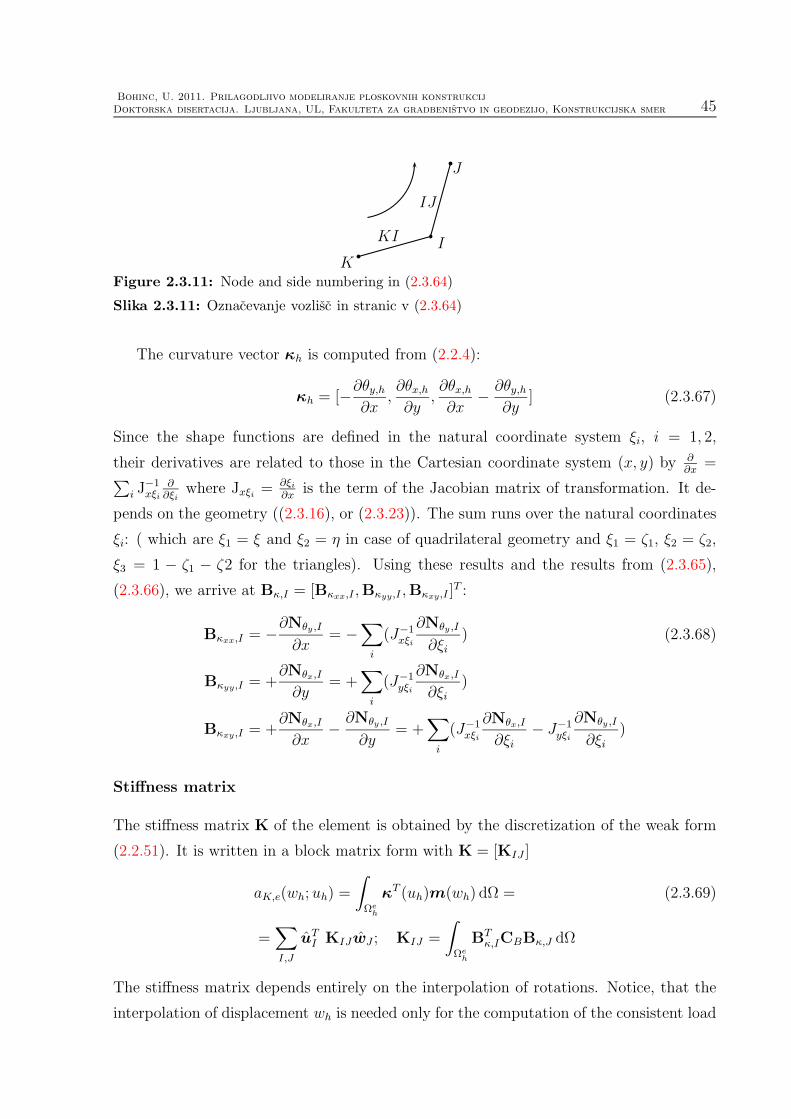
Bohinc, U. 2011. Prilagodljivo modeliranje ploskovnih konstrukcij
Doktorska disertacija. Ljubljana, UL, Fakulteta za gradbenistvo in geodezijo, Konstrukcijska smer 45
KI
J
KI
IJ
Figure 2.3.11: Node and side numbering in (2.3.64)
Slika 2.3.11: Oznacevanje vozlisc in stranic v (2.3.64)
The curvature vector κh is computed from (2.2.4):
κh = [−∂θy,h∂x
,∂θx,h∂y
,∂θx,h∂x
− ∂θy,h∂y
] (2.3.67)
Since the shape functions are defined in the natural coordinate system ξi, i = 1, 2,
their derivatives are related to those in the Cartesian coordinate system (x, y) by ∂∂x
=∑
i J−1xξi
∂∂ξi
where Jxξi =∂ξi∂x
is the term of the Jacobian matrix of transformation. It de-
pends on the geometry ((2.3.16), or (2.3.23)). The sum runs over the natural coordinates
ξi: ( which are ξ1 = ξ and ξ2 = η in case of quadrilateral geometry and ξ1 = ζ1, ξ2 = ζ2,
ξ3 = 1 − ζ1 − ζ2 for the triangles). Using these results and the results from (2.3.65),
(2.3.66), we arrive at Bκ,I = [Bκxx,I ,Bκyy,I ,Bκxy,I ]T :
Bκxx,I = −∂Nθy ,I
∂x= −
∑
i
(J−1xξi
∂Nθy ,I
∂ξi) (2.3.68)
Bκyy,I = +∂Nθx,I
∂y= +
∑
i
(J−1yξi
∂Nθx,I
∂ξi)
Bκxy,I = +∂Nθx,I
∂x− ∂Nθy ,I
∂y= +
∑
i
(J−1xξi
∂Nθx,I
∂ξi− J−1
yξi
∂Nθy ,I
∂ξi)
Stiffness matrix
The stiffness matrix K of the element is obtained by the discretization of the weak form
(2.2.51). It is written in a block matrix form with K = [KIJ ]
aK,e(wh; uh) =
∫
Ωeh
κT (uh)m(wh) dΩ = (2.3.69)
=∑
I,J
uTI KIJwJ ; KIJ =
∫
Ωeh
BTκ,ICBBκ,J dΩ
The stiffness matrix depends entirely on the interpolation of rotations. Notice, that the
interpolation of displacement wh is needed only for the computation of the consistent load

46Bohinc, U. 2011. Adaptive modeling of plate structures
Doctoral thesis. Cachan, ENS Cachan, LMT
1
2
3
w1
θx,1, θy,1
Figure 2.3.12: Triangular DK plate element - DK
Slika 2.3.12: Trikotni DK koncni element za plosce - DK
vector f . The explicit form of the displacement interpolation for the DK element was
first obtained in [Ibrahimbegovic, 1993].
Load vector
From (2.2.50) we have
lK,e(uh) =∑
I
uTI fI = uTf = (2.3.70)
=
∫
Ωeh
f uhdΩ +∑
ΓeIJ
[∫
ΓeIJ
(qef uh +ms θh(uh) · s) ds+ [mnuh,Γ]JI
]
ff,I =
∫
Ωeh
f Nw,IdΩ; ft,I =∑
Γe,IJ
∫
Γe,IJ
(qefNw,I +ms sTNθ,I) ds
The consistent nodal load vector is fI = ff,I + ft,I .
Triangular DK plate element - DKT
The DKT element has three vertex nodes with nodal degrees of freedom uI = [wI , θxI , θyI ].
The shape functions are formulated in the area coordinates:
NI = ζI ; NIJ = 4ζIζJ ; MIJ = 4ζIζJ(ζJ − ζI) (2.3.71)
The side between the nodes I and J is denoted by IJ . The shape functions (2.3.71) match
the hierarchical shape functions (2.3.55) on the sides of the element. To show this, let us

Bohinc, U. 2011. Prilagodljivo modeliranje ploskovnih konstrukcij
Doktorska disertacija. Ljubljana, UL, Fakulteta za gradbenistvo in geodezijo, Konstrukcijska smer 47
Table 2.3: 4 point triangular integration scheme for triangular finite elements (DKT)
Tabela 2.3: 4 tockovna integracijska shema za trikotne koncne elemente (DKT)
ζ1 ζ1 ζ1 wi
1 1/3 1/3 1/3 -27/48
2 3/5 1/5 1/5 25/48
3 1/5 3/5 1/5 25/48
4 1/5 1/5 3/5 25/48
denote the coordinate along the side IJ by ξ ∈ [−1,+1]. On ΓIJ we have
NI = ζI = (1− ξ)/2; NJ = ζJ = (1 + ξ)/2 (2.3.72)
Inserting the expressions for NI and NJ into (2.3.71), we recover
NIJ = (1− ξ2); MIJ = (1− ξ2)ξ (2.3.73)
A 4-point triangular scheme for the numerical integration is used in this work to com-
pute stiffness matrix and load vector of DKT element (2.3.69), (2.3.70) (see [Zienkiewicz
Taylor, 2000]). The coordinates of the integration points and the weights wi are listed in
Table 2.3.
The quadrilateral DK plate element - DKQ
The DKQ element has four vertex nodes with nodal degrees of freedom uI = [wI , θxI , θyI ].
The shape functions are constructed directly from the hierarchical shape functions (2.3.55).
The compact definition of the shape functions is formulated in the natural coordinate sys-
tem (ξ, η) ∈ [−1,+1]× [−1,+1]:
I 1 2 3 4IJ 12 23 34 41r ξ η ξ ηs η ξ η ξpr +1 +1 -1 -1ps +1 -1 -1 +1
NI = (1− prr)(1− pss)/4; (2.3.74)
NIJ = (1− r2)(1− pss)/2;
MIJ = prr(1− r2)(1− pss)/2
The shape functions are depicted in Figure 2.3.14. A 2 × 2 Gauss scheme is used for
the numerical integration to compute stiffness matrix and load vector of DKQ element
(2.3.69), (2.3.70) (see [Zienkiewicz Taylor, 2000]). The coordinates of the integration
points and the weights wi are listed in Table 2.4.

48Bohinc, U. 2011. Adaptive modeling of plate structures
Doctoral thesis. Cachan, ENS Cachan, LMT
Figure 2.3.13: Hierarchic shape functions of the triangular DK plate elementSlika 2.3.13: Hierarhicne interpolacijske funkcije trikotnega DK elementa
Table 2.4: 4 point quadrilateral integration scheme for quadrilateral finite elements (DKQ)
Tabela 2.4: 4 tockovna integracijska shema za stirikotne koncne elemente (DKQ)
ξ η wi
1 −1/√3 −1/
√3 1
2 +1/√3 −1/
√3 1
3 +1/√3 +1/
√3 1
4 −1/√3 +1/
√3 1

Bohinc, U. 2011. Prilagodljivo modeliranje ploskovnih konstrukcij
Doktorska disertacija. Ljubljana, UL, Fakulteta za gradbenistvo in geodezijo, Konstrukcijska smer 49
Figure 2.3.14: Hierarchic shape functions of the quadrilateral DK plate elementSlika 2.3.14: Hierarhicne interpolacijske funkcije stirikotnega koncnega elementa za plosceDKQ

50Bohinc, U. 2011. Adaptive modeling of plate structures
Doctoral thesis. Cachan, ENS Cachan, LMT
2.4 Examples
The purpose of presented numerical examples is two-folds: (i) to illustrate specific issues
involved in plate modeling and (ii) to compare the performance of finite elements that will
be later used for discretization and model error estimation in different situations. The
finite element solutions are compared to the reference ones. Where possible, the reference
solutions are obtained analytically (in closed form or in the form of series expansion). In
the cases where the analytical solution is not available, a finite element solution obtained
with the most enhanced element on a very fine mesh presents the reference solution. In
the figures, the nomenclature of Figure 2.4.1 is employed.
The presented finite elements were implemented in the Fortran based finite element
program FEAP [Taylor, 2000], developed by R. Taylor. They were also implemented in
the C++ based finite element program AceFEM [Korelc, 2006], developed by J. Korelc.
In the later implementation the symbolic manipulation code AceGEN [Korelc, 2006],
developed by J. Korelc, was used. Additional routines, used for postprocessing were
coded in Mathematica [Wolfram, 1988] and Matlab [Guide, 1998].
The computed FE stress resultants are not continuous across element boundaries,
which makes the assessment of the results difficult. To produce readable plots of stress
resultants, the nodal values are computed from the element integration point values using
the standard averaging technique, see [Taylor], section 5.5. The shear forces are computed
from the equilibrium equations (2.2.17). They depend on the derivatives of the moment
resultants. To obtain the derivatives, the bilinear interpolation of moment resultants on
Ωeh is first built from the integration point values. The equilibrium shear forces are indexed
by ,e in the FE plots to distinguish them from the constitutive shear forces.
Surface load
Hard simple support
Soft simple support
Clamped
Figure 2.4.1: Designation of boundary conditions and loadsSlika 2.4.1: Oznake robnih pogojev in obtezb

Bohinc, U. 2011. Prilagodljivo modeliranje ploskovnih konstrukcij
Doktorska disertacija. Ljubljana, UL, Fakulteta za gradbenistvo in geodezijo, Konstrukcijska smer 51
2.4.1 Uniformly loaded simply supported square plate
A simply supported rectangular plate of side length a = 10 and thickness t = 0.01 under
uniform loading f = 1 is considered. The material is linear elastic and isotropic, with
Young’s modulus E = 10.92 × 10¹⁰ and Poisson’s ratio ν = 0.3. The plate support is
modeled as a hard simple support: the rotation θn at the sides of the plate is set to
zero.
x
y
a
a
E,ν,t,f
Figure 2.4.2: Problem definition and geometry for the uniformly loaded simply supportedsquare plate (t/a=1/1000)Slika 2.4.2: Definicija in geometrija problema enakomerno obremenjene prosto podprtekvadratne plosce (t/a=1/1000)
Reference solution
Since the plate is very thin (a/t=1000), the solution of the Kirchhoff theory is considered
as the reference one. The bi-harmonic equation (2.2.26) is solved by the analytical function
in the form of series expansion, see e.g. [Timoshenko Vojnovski-Kriger, 1959]:
w =f
D
16
π6
∞∑
m=1
∞∑
n=1
sin(nπ xa) sin(mπ y
b)
mn ((na)2 + (m
b)2)2
; m = 1, 3, 5, · · · n = 1, 3, 5, · · ·
where a, b are the sides of the plate and D = Et3
12(1−ν2)is the plate bending stiffness. At
the center of the square plate b = a; x = y = a/2, we have:
w =fa4
D
0.0040623532︷ ︸︸ ︷16
π6
∞∑
m=1
∞∑
n=1
sin(nπ2) sin(mπ
2)
mn(n2 +m2)2(2.4.1)
m =1, 3, 5, · · · n = 1, 3, 5, · · ·
52Bohinc, U. 2011. Adaptive modeling of plate structures
Doctoral thesis. Cachan, ENS Cachan, LMT
The curvatures are computed from κ = [∂2w
∂x2 ,∂2w∂y2
, 2 ∂2w∂x∂y
]T and moment resultants from
m = CBκ, where CB is the constitutive matrix. At the geometrical center of the rectan-
gular plate, the moment resultants are
mxx = −0.0368381 (1− ν)qa2; myy = −0.0368381 (1− ν)qa2; mxy = 0
and at the corners of the plate
mxx = 0; myy = 0; mxy = ±0.0463741 (1− ν)qa2
The reference solution is shown in Figure 2.4.3. It contains contour plots of the
displacement w and the rotations θx, θy. In the second column, the moment resultants
mxx, myy and mxy are shown. The third column contains the contour plots of equilibrium
shear forces qx and qy. The solution is regular throughout the domain and does not exhibit
any singularities.
Finite element solutions
The problem is solved with the conforming finite element ARGY and the nonconforming
discrete Kirchhoff elements DKT and DKQ. All the solutions are obtained on a similar
mesh. A rather coarse mesh is used in order to be able to clearly distinguish the differences
between the solutions obtained with various finite elements. The hard-simple supports
are modeled by constraining (setting to zero) the nodal displacements wI and rotations
θn,I . When using Argyris element, additionally the nodal curvatures κxx,I and κyy,I are
set to zero. In the mid-side nodes lying at the supported edges the nodal normal slope
w,n|I is left free.
Figures 2.4.4 and 2.4.5 show FE solutions. The comparison of FE solutions obtained
with Argyris and DK elements shows good agreement with the reference solution. Since
the range (and the color coding) in Figures 2.4.3, 2.4.4 and 2.4.5 is the same, it is possible
to visually asses the differences of the FE solutions. In the current case, the differences
between the solutions are, however, minor.
More quantitative comparison of element performance is shown in Figure (2.4.6), where
a study of element performance versus mesh density is presented. The plots show the log-
log plot of relative error of several selected quantities versus the total number of degrees
of freedom (both constrained and unconstrained) which is inversely proportional to the
average element size. The a-apriori estimate of the convergence rate is hp, where h is
the average size of the element and p the interpolation order. In the log-log plot, the

Bohinc, U. 2011. Prilagodljivo modeliranje ploskovnih konstrukcij
Doktorska disertacija. Ljubljana, UL, Fakulteta za gradbenistvo in geodezijo, Konstrukcijska smer 53
convergence lines are straight lines. The slope of the lines in the log-log plot indicates
the rate of convergence. The comparison of Argyris and DK elements clearly shows
the superior convergence rate of the Argyris element in all of the studied quantities:
displacement w and momentmxx at the center of the plate as well as the total deformation
energy of the plate, defined as W int =∑
e
∫Ωe
h
κTCBκdΩ. The integrand is evaluated at
integration points and numerically integrated. Convergence of W int is not monotone for
the case of ARGY element which explains a kink in the convergence plot. The effect can
be attributed to the choice of the numerical integration scheme. The superconvergent
points of the ARGY element are the element nodes, while the integration points of the
triangular integration scheme (2.3) lie in the interior of the element domain.
The convergence rate for the ARGY element is roughly twice as higher as the conver-
gence rate of DK elements.
2.4.2 Uniformly loaded clamped square plate
A rectangular plate of side length a = 10 and thickness t = 0.01 under uniform loading
f = 1 is analyzed. All sides of the plates are clamped. The material is linear elastic and
isotropic, with Young’s modulus E = 10.92× 10¹⁰ and Poisson’s ratio ν = 0.3.
a
a
x
y
E,ν,t,f
Figure 2.4.7: Problem definition and geometry for the uniformly loaded clamped square plate(t/a=1/1000)Slika 2.4.7: Definicija in geometrija enakomerno obremenjene vpete kvadratne plosce(t/a=1/1000)

54Bohinc, U. 2011. Adaptive modeling of plate structures
Doctoral thesis. Cachan, ENS Cachan, LMT
Reference solution
The reference solution is the analytical solution in the form of series expansion. Since
the series converges quite slowly, a special treatment is necessary to be able to efficiently
compute the reference result (see e.g. [Taylor Govindjee, 2002]). The main results are
given at the center of the plate:
w = 1.26531908710−3fa4
D; mxx = −2.29050835210−2fa2 (2.4.2)
The total deformation energy is W int = 3.89120077510−4 f2a4
D. In this work we use the
above results with the material and geometry data as given above.
Finite element solutions
FE solutions are shown in Figure 2.4.9 and Figure 2.4.10. The boundary conditions for
DK elements were w = 0, θx,I = 0 and θy,I = 0 at the clamped sides of the plate. The
boundary conditions for the ARGY elements were w = 0, w,x = 0, w,y = 0 at the vertex
nodes and w,n = 0 at the midside nodes.
The qualitative comparison does not reveal any significant differences in the perfor-
mance of the elements. However, the difference becomes clearly visible, when the con-
vergence is observed (see Figure 2.4.11). The convergence of the ARGY element is one
order higher that that of DK elements. Notice, however, that for the very coarse mesh,
the results of both type of elements are quite comparable.
2.4.3 Uniformly loaded clamped circular plate
A clamped circular plate of radius R = 5 and thickness t = 0.01 under uniform loading
f = 1 is considered. The material is linear elastic and isotropic, with Young’s modulus
E = 6.825× 10⁹ and Poisson’s ratio ν = 0.3.

Bohinc, U. 2011. Prilagodljivo modeliranje ploskovnih konstrukcij
Doktorska disertacija. Ljubljana, UL, Fakulteta za gradbenistvo in geodezijo, Konstrukcijska smer 55
R
x
y
E,ν,t,f
Figure 2.4.12: Clamped circular plate with uniform load (t/R=1/500)Slika 2.4.12: Enakomerno obremenjena vpeta krozna plosca (t/R=1/500)
Reference solution
By taking into account the symmetry, it is possible to obtain the closed form solution of
the problem (see [Timoshenko Vojnovski-Kriger, 1959]). The displacement of uniformly
loaded clamped circular plate is defined by:
w = f(R2 − r2)2/64/D (2.4.3)
The moment resultants at the center of the plate are:
mxx = − 1
16fR2/D(1 + ν); myy = − 1
16fR2(1 + ν); mxy = 0 (2.4.4)
In current case, where we have D = R4 = 625, the displacement at the enter is w =
1/64 = 0.015625 and moment resultant mxx = −25/16 ∗ 1.3 = −2.03125.
Finite element solutions
A quarter of of the plate is modeled in FE analyses. The symmetry boundary conditions
are taken into account at x = 0 and y = 0. The boundary conditions are listed in (2.4.5).
DK wI θx,I θy,Ix = 0 - - 0y = 0 - 0 -r = R 0 0 0
ARGY wI wI,x wI,y wI,xx wI,yy wI,xy wI−J,n
x = 0 - - 0 - - 0 0y = 0 - 0 - - - 0 0r = R 0 0 0 - - - 0
(2.4.5)
The meshes were constructed so, that the distortion of the elements was minimized. In
the case of quadrilateral elements, the distortion of the elements is, however, still signifi-
cant. The sequence of meshes used in the convergence analysis is shown in Figure 2.4.14.

56Bohinc, U. 2011. Adaptive modeling of plate structures
Doctoral thesis. Cachan, ENS Cachan, LMT
Notice that the area of the FE problem domain Ωh converges to the area Ω as the mesh
is refined. As shown in Figure 2.4.15, the FE solution with ARGY element shows very
good qualitative agreement with the reference solution. Results of the DK elements are
being influenced by the mesh distortion (quadrilaterals) and mesh orientation (triangles).
The influence is, however, noticeable only when the comparison of the equilibrium shear
forces with the reference solution is made. One can thus conclude that the mesh distor-
tion (quadrilaterals) and mesh orientation (triangles) has the greatest influence on the
computation of the transverse shear forces.
The comparison of the convergence, shown in Figure 2.4.17, reveals an interesting fact.
The convergence of the ARGY element is no longer superior to that of DK elements, but
is rather of the same order. This can be attributed to the fact, that the error made in the
approximation of the curved domain boundary dominates the overall error.

Bohinc, U. 2011. Prilagodljivo modeliranje ploskovnih konstrukcij
Doktorska disertacija. Ljubljana, UL, Fakulteta za gradbenistvo in geodezijo, Konstrukcijska smer 57
Figure
2.4.3:Referen
cesolution
oftheuniformly
load
edsimply
supportedsquareplate
withlegendalso
validforFigures2.4.4an
d2.4.5
Slika2.4.3:Referencn
aresiteven
akom
ernoob
remen
jeneprostopodprtekvadratneplosce
zlegendo,
kiveljatudiza
Sliki2.4.4in
2.4.5

58Bohinc, U. 2011. Adaptive modeling of plate structures
Doctoral thesis. Cachan, ENS Cachan, LMT
(ARGY
element)
Figure
2.4.4:FE
solution
oftheuniform
lyload
edsim
ply
supported
square
plate
with
Argy
risplate
element
Slik
a2.4.4:Racu
nska
resiteven
akomern
oob
remen
jeneprosto
podprte
kvad
ratneplosce
zArgy
risovim
koncn
imelem
entom

Bohinc, U. 2011. Prilagodljivo modeliranje ploskovnih konstrukcij
Doktorska disertacija. Ljubljana, UL, Fakulteta za gradbenistvo in geodezijo, Konstrukcijska smer 59
(DKT
elem
ent)
(DKQ
elem
ent)
Figure
2.4.5:Finiteelem
entsolution
oftheuniformly
load
edsimply
supportedsquareplate
withDK
plate
elem
ents
Slika2.4.5:Racunskaresiteven
akom
ernoob
remen
jeneprostopodprtekvadratneploscezDK
koncn
imielem
enti

60Bohinc, U. 2011. Adaptive modeling of plate structures
Doctoral thesis. Cachan, ENS Cachan, LMT
(Displacement w at center)
(Moment resultant mxx at center)
(Energy norm)
Figure 2.4.6: Comparison of the convergence of FE solutions for the uniformly loaded simplysupported square plateSlika 2.4.6: Primerjava konvergence racunske resitve problema enakomerno obremenjene prostopodprte kvadratne plosce

Bohinc, U. 2011. Prilagodljivo modeliranje ploskovnih konstrukcij
Doktorska disertacija. Ljubljana, UL, Fakulteta za gradbenistvo in geodezijo, Konstrukcijska smer 61
Figure
2.4.8:Referen
cesolution
oftheuniformly
load
edclam
ped
squareplate
withlegendalso
validforFigures2.4.9an
d2.4.10
Slika2.4.8:Referencn
aresiteven
akom
ernoob
remen
jenevpetekvadratneplosce
zlegendo,
kiveljatudiza
Sliki2.4.9in
2.4.10

62Bohinc, U. 2011. Adaptive modeling of plate structures
Doctoral thesis. Cachan, ENS Cachan, LMT
(ARGY
element)
Figure
2.4.9:FE
solution
oftheuniform
lyload
edclam
ped
square
plate
with
Argy
risplate
element
Slik
a2.4.9:Racu
nska
resiteven
akomern
oob
remen
jenevpete
kvad
ratneplosce
zArgy
risovim
koncn
imelem
entom

Bohinc, U. 2011. Prilagodljivo modeliranje ploskovnih konstrukcij
Doktorska disertacija. Ljubljana, UL, Fakulteta za gradbenistvo in geodezijo, Konstrukcijska smer 63
(DKT
elem
ent)
(DKQ
elem
ent)
Figure
2.4.10:FE
solution
oftheuniformly
load
edclam
ped
squareplate
withDK
plate
elem
ents
Slika2.4.10:Racunskaresiteven
akom
ernoob
remen
jenevpetekvadratneploscezDK
koncn
imielem
enti
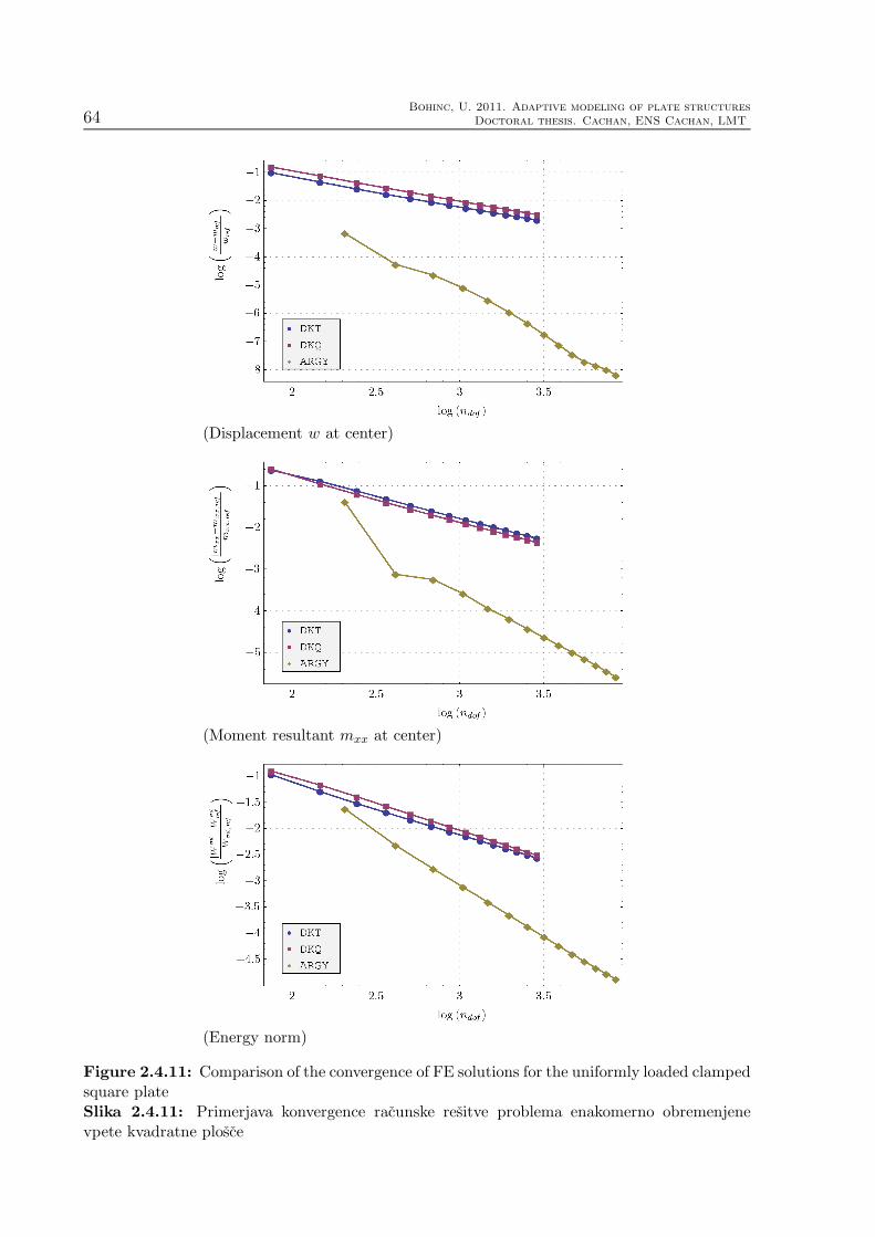
64Bohinc, U. 2011. Adaptive modeling of plate structures
Doctoral thesis. Cachan, ENS Cachan, LMT
(Displacement w at center)
(Moment resultant mxx at center)
(Energy norm)
Figure 2.4.11: Comparison of the convergence of FE solutions for the uniformly loaded clampedsquare plateSlika 2.4.11: Primerjava konvergence racunske resitve problema enakomerno obremenjenevpete kvadratne plosce

Bohinc, U. 2011. Prilagodljivo modeliranje ploskovnih konstrukcij
Doktorska disertacija. Ljubljana, UL, Fakulteta za gradbenistvo in geodezijo, Konstrukcijska smer 65
Figure
2.4.13:Referen
cesolution
oftheuniformly
load
edclam
ped
circularplate
withlegendalso
validforFigures2.4.15
and2.4.16
Slika2.4.13:Referencn
aresiteven
akom
ernoob
remen
jenevpetekrozn
eplosce
zlegendo,
kiveljatudiza
Sliki2.4.15
in2.4.16

66Bohinc, U. 2011. Adaptive modeling of plate structures
Doctoral thesis. Cachan, ENS Cachan, LMT
(Sequence of meshes of triangular elements)
(Sequence of meshes of quadrilateral elements)
Figure 2.4.14: The sequence of meshes used for the finite element solution of uniformly loadedclamped circular plateSlika 2.4.14: Zaporedje mrez uporabljenih pri resitvi enakomerno obremenjene vpete krozneplosce

Bohinc, U. 2011. Prilagodljivo modeliranje ploskovnih konstrukcij
Doktorska disertacija. Ljubljana, UL, Fakulteta za gradbenistvo in geodezijo, Konstrukcijska smer 67
(ARGY
elem
ent)
Figure
2.4.15:FE
solution
oftheuniformly
load
edclam
ped
circularplate
withArgyrisplate
elem
ent
Slika2.4.15:Racunskaresiteven
akom
ernoob
remen
jenevpetekrozn
eploscezArgyrisovim
koncn
imelem
entom

68Bohinc, U. 2011. Adaptive modeling of plate structures
Doctoral thesis. Cachan, ENS Cachan, LMT
(DKT
element)
(DKQ
element)
Figure
2.4.16:FE
solution
oftheuniform
lyload
edclam
ped
circular
plate
with
DK
plate
elements
Slik
a2.4.16:Racu
nska
resiteven
akomern
oob
remen
jenevpete
krozn
eplosce
zDK
koncn
imielem
enti

Bohinc, U. 2011. Prilagodljivo modeliranje ploskovnih konstrukcij
Doktorska disertacija. Ljubljana, UL, Fakulteta za gradbenistvo in geodezijo, Konstrukcijska smer 69
(Displacement w at center)
(Moment resultant mxx at center)
(Energy norm)
Figure 2.4.17: Comparison of the convergence of FE solutions for the uniformly loaded clampedcircular plateSlika 2.4.17: Primerjava konvergence racunske resitve problema enakomerno obremenjenevpete krozne plosce

70Bohinc, U. 2011. Adaptive modeling of plate structures
Doctoral thesis. Cachan, ENS Cachan, LMT
2.4.4 Uniformly loaded hard simply supported skew plate
The analysis of Morley’s α = 30 skew plate under uniform loading f = 1 with thickness
t = 0.1 and side length a = 10 is considered. The plate is hard simply supported on all
sides. The Young’s modulus is E = 10.92× 10⁷ and Poisson’s ratio is ν = 0.3.
x
y
a
aα = π/6
E,ν,t,f
Figure 2.4.18: Problem definition and geometry for the uniformly loaded simply supportedskew plate (t/a=100)Slika 2.4.18: Definicija in geometrija problema enakomerno obremenjene prosto podprte rom-boidne plosce (t/a=1/100)
Reference solution
The most interesting feature of the solution concerns two singular points at the two obtuse
corners of the plate, which strongly influence the quality of the computed results (e.g. see
[Morley, 1963]). The strength of the singularity is λ = 6/5 = 1.2 see (2.2.66). In the
vicinity of the corner, the moment resultants mxx, myy vary as rλ−2, while the moments
resultant mxy and shear forces qx and qy vary as rλ−3, where r is the distance from the
corner. As the analytic solution is not available, a finite element computation with Argyris
element on a fine mesh (the elements with side h = 0.1) is taken as the reference solution.
The reference solution confirms the existence of the singularity in the obtuse corners.
Finite element solutions
The boundary conditions used for the hard simply supported edge at y = const. are:
wI = 0, θx,I = 0 for DK elements and wI = 0, wI,x = 0 for the ARGY element. At the
hard simply supported sloped edge y/x = tanα the rotation θn is set to zero, which results
in the boundary condition: θx,I − tanα θy,I = 0 for DK elements and wI,y+tanα wI,x = 0.
The finite element solutions with ARGY element is shown in Figure 2.4.20. A serious
deterioration of the accuracy is observed at the obtuse corners. In order to capture the

Bohinc, U. 2011. Prilagodljivo modeliranje ploskovnih konstrukcij
Doktorska disertacija. Ljubljana, UL, Fakulteta za gradbenistvo in geodezijo, Konstrukcijska smer 71
Figure 2.4.19: Reference solution of the uniformly loaded simply supported skew platewith legend also valid for Figures 2.4.20 and 2.4.21Slika 2.4.19: Referencna resitev enakomerno obremenjene prosto podprte romboidne ploscez legendo, ki velja tudi za Sliki 2.4.20 in 2.4.21
singularity better, the density of the mesh has to be increased at the obtuse corners. The
finite element solution with DK elements qualitatively matches the reference solution in
problem domain except at the obtuse corners. The quality of the finite element solution
is influenced by the mesh distortion (see Figure 2.4.22). The performance of triangular
element DKT does not the reach the performance of the quadrilateral element DKQ. The
comparison of the converge rates shows, surprisingly, that the superior accuracy of the
ARGY element, which was observed in the previous tests, is now lost.
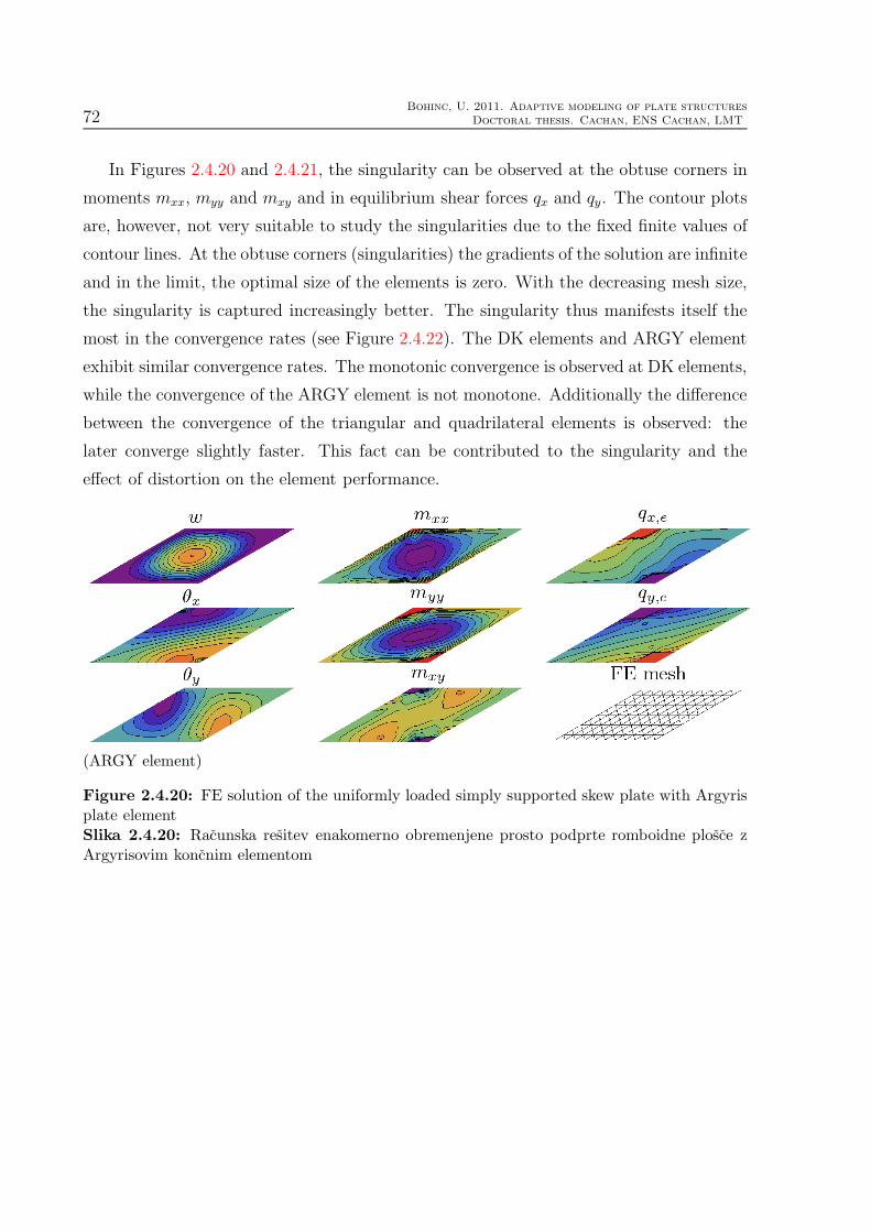
72Bohinc, U. 2011. Adaptive modeling of plate structures
Doctoral thesis. Cachan, ENS Cachan, LMT
In Figures 2.4.20 and 2.4.21, the singularity can be observed at the obtuse corners in
moments mxx, myy and mxy and in equilibrium shear forces qx and qy. The contour plots
are, however, not very suitable to study the singularities due to the fixed finite values of
contour lines. At the obtuse corners (singularities) the gradients of the solution are infinite
and in the limit, the optimal size of the elements is zero. With the decreasing mesh size,
the singularity is captured increasingly better. The singularity thus manifests itself the
most in the convergence rates (see Figure 2.4.22). The DK elements and ARGY element
exhibit similar convergence rates. The monotonic convergence is observed at DK elements,
while the convergence of the ARGY element is not monotone. Additionally the difference
between the convergence of the triangular and quadrilateral elements is observed: the
later converge slightly faster. This fact can be contributed to the singularity and the
effect of distortion on the element performance.
(ARGY element)
Figure 2.4.20: FE solution of the uniformly loaded simply supported skew plate with Argyrisplate elementSlika 2.4.20: Racunska resitev enakomerno obremenjene prosto podprte romboidne plosce zArgyrisovim koncnim elementom

Bohinc, U. 2011. Prilagodljivo modeliranje ploskovnih konstrukcij
Doktorska disertacija. Ljubljana, UL, Fakulteta za gradbenistvo in geodezijo, Konstrukcijska smer 73
(DKT element)
(DKQ element)
Figure 2.4.21: FE solution of the uniformly loaded simply supported skew plate with DKplate elementsSlika 2.4.21: Racunska resitev enakomerno obremenjene prosto podprte romboidne plosce zDK koncnimi elementi

74Bohinc, U. 2011. Adaptive modeling of plate structures
Doctoral thesis. Cachan, ENS Cachan, LMT
(Displacement w at center)
(Moment mxx at center)
(Energy norm)
Figure 2.4.22: Comparison of the convergence of FE solutions for the uniformly loaded simplysupported skew plateSlika 2.4.22: Primerjava konvergence racunske resitve problema enakomerno obremenjeneprosto podprte romboidne plosce

Bohinc, U. 2011. Prilagodljivo modeliranje ploskovnih konstrukcij
Doktorska disertacija. Ljubljana, UL, Fakulteta za gradbenistvo in geodezijo, Konstrukcijska smer 75
2.5 Chapter summary and conclusions
In this chapter, we studied and revisited the theory of the (thin) Kirchhoff plate model
and derived several finite element formulations based on that model. The motivation
to dedicate some effort to study in more detail the well known topic - the Kirchhoff
plate theory - is strongly connected to the main goals of this thesis. The main goals
of the thesis are namely related to the derivation of procedures for discretization error
estimation and model error estimation in the process of the finite element computation
of plate-like structure.
As it will be explained in the following chapters, both discretization error estimation
and model error estimation can be performed by a comparison of numerical results that
are obtained by using two different level of complexities in the computations. In the
model error estimation, the complexity is associated with the type of the used hierarchical
plate model (i.e. thin, moderately thick, thick). Those models are covered in the first
three chapters. On the other hand, in the discretization error estimation, the complexity
is associated with the type of finite element formulation (less rigorous, more rigorous)
within the framework of a single plate model.
Due to the above reasons, the thin plate model (theory) was studied in some detail in
the first part of this chapter. The topis, like strong form of the boundary value problem,
and singularities of solution, which may not be very familiar to those dealing with finite
element computations of plates, were considered in order to prepare ourselves for better
understanding of problems that might pop-up when dealing with discretization and model
error of plates.
In the second part of this chapter, several finite elements were derived. First, a con-
forming triangular element with 21 dofs was presented in detail. This element has not
been used by the engineers, although, due to its completeness, it is relatively popular by
mathematicians dealing with the plate problems (e.g. [Bernadou, 1996]). This element is
very rigorous with respect of taking into account assumptions of Kirchhoff plate model.
Next, triangular and quadrilateral discrete Kirchhoff plate elements were rederived. Those
elements are more relaxed with respect to the Kirchhoff plate theory assumptions than
the conforming one. The elements perform very well in general and may be found in many
commercial finite element codes (e.g. [Wilson, 1997]).
The chapter concludes with the numerical examples, where the results obtained by the
three above mentioned elements are compared by each other and by reference analytical

76Bohinc, U. 2011. Adaptive modeling of plate structures
Doctoral thesis. Cachan, ENS Cachan, LMT
solutions. As expected, the conforming element shows superiority to the DK elements.
In summary, this chapter deals with the thin plate theory and some corresponding
finite element formulations that are of our interest for the later purpose. The main novelty
of this chapter can be related to the nonconventional notation in the derivation of the DK
elements, which is such, that both triangular and quadrilateral element formulations can
be covered by using a single notation.

Bohinc, U. 2011. Prilagodljivo modeliranje ploskovnih konstrukcij
Doktorska disertacija. Ljubljana, UL, Fakulteta za gradbenistvo in geodezijo, Konstrukcijska smer 77
Chapter 3
Moderately thick plates: theory andfinite element formulations
3.1 Introduction
The theory of moderately thick plates, in contrast to the Kirchhoff plate theory, takes into
account transverse shear deformations. The Kirchhoff constraint is relaxed. Therefore, an
additional freedom exists for the modes of deformation. A relaxation of the assumptions
of the Kirchhoff theory was first made by [Reissner, 1945] and later, in a slightly different
manner, by [Mindlin, 1951]. Since Reissner and Mindlin theories are not very different,
it is common to denote a theory for plates with moderate thickness as a theory of Reiss-
ner/Mindlin type. An analogy exists between the Euler-Bernoulli and the Timoshenko
beam theories and Kirchhoff and Reissner/Mindlin plate theories, respectively.
In the Kirchhoff theory, the rotation of the plate normal is completely defined by the
displacement of the midsurface, whereas in the Reissner/Mindlin plate theory it is inde-
pendent of displacement. The independence of rotations and transverse displacement has
several consequences. The continuity of the rotations is no longer required and Reiss-
ner/Mindlin plate loaded with a line load, can have kinks with abrupt change of slope.
On the other hand, a point load, which produces in Kirchhoff plate finite displacement
exhibits singularity in the Reissner/Mindlin plate. Perhaps the most interesting manifes-
tation of the additional freedom, gained by the relaxation of Kirchhoff constraint, is the
existence of a boundary layers - a region of a plate close to the boundary, where quick and
significant changes in twisting moment and shear forces occur. The boundary effect, how-
ever, is not only a consequence of the assumptions of the Reissner/Mindlin plate theory,
but rather a real physical phenomenon.
In Reissner/Mindlin treatment of plate bending the basic assumptions are: (i) the

78Bohinc, U. 2011. Adaptive modeling of plate structures
Doctoral thesis. Cachan, ENS Cachan, LMT
material normal to the original reference surface remains straight, although no longer
normal to the deformed reference surface, (ii) the thickness of the plate does not change
during deformation and (iii) transverse normal stresses are negligible. The latter two
assumptions are contradictory, which can easily be verified. Reissner and Mindlin plate
theories differ from each other in a way how they solve this problem. While Reissner
assumed a cubic variation in thickness direction of transverse normal stress, Mindlin ma-
nipulated the material law in order to comply with both assumptions [Reissner, 1945],
[Mindlin, 1951]. Although conceptionally different, both plate theories deliver practically
the same results for transverse displacements, shear forces and bending moments in ac-
tual structural problems. The basic consequence of the above assumptions is that the
deformation of the moderately thick plate can no longer be defined by the transverse
displacement w and its derivatives only. The rotation of material normal θ is introduced
as an independent variable.
3.2 Theory
3.2.1 Governing equations
Kinematics
In the following, the rotation φ will be employed instead of the conventional rotation
θ, see Figure 2.2.1. Recall that the rotations are related as φ = [φx, φy]T = [−θy , θx]T .
According to (2.2.3) and (2.2.4), the kinematic relations, which relate the displacement
w and rotation φ to the curvatures κ = [κxx, κyy, κxy]T and transverse shear strains
γ = [γx, γy]T , are
κ = [∂φx
∂x,∂φy
∂y, (∂φy
∂x+∂φx
∂y)]T ; γ = [
∂w
∂x− φx,
∂w
∂y− φy]
T (3.2.1)
In a compact notation we have
γ = ∇w − φ; κ = Dφ (3.2.2)
where the differential operator D is
D =
∂∂x
0
0 ∂∂y
∂∂y
∂∂x
(3.2.3)

Bohinc, U. 2011. Prilagodljivo modeliranje ploskovnih konstrukcij
Doktorska disertacija. Ljubljana, UL, Fakulteta za gradbenistvo in geodezijo, Konstrukcijska smer 79
Equilibrium equations
The equilibrium equations were derived already in the previous chapter. We recall the
main result:
∇ · qeq = −f (3.2.4)
where the shear forces obtained from the equilibrium equations are denoted in this chapter
as qeq = [qx,eq, qy,eq]T . We also recall from (2.2.18):
∇ ·M = −qeq; M =
[mxx mxy
mxy myy
](3.2.5)
Constitutive relations
To obtain the moment-curvature relationship, we recall from (2.2.12) and (2.2.13): the
moments are related to curvatures as
m = CBκ (3.2.6)
The kinematic shear strains γ computed from the kinematic assumptions (3.2.1) are
constant through the thickness, which is approximation to the actual variation, even for
a homogeneous cross-section. The equilibrium equations show, that the variation of the
shear stresses through the thickness must exist. For the homogeneous cross-sections, the
shear strain distribution is commonly accepted to be a parabolic function of z.
Strains following from the kinematic assumptions are in contrast with the equilibrium
of differential plate element. To overcome this difficulty, two theories were presented
([Reissner, 1945] and [Mindlin, 1951]), both resulting in the introduction of the shear
correction factor c which enables the definition of the following simplified constitutive
relation, where the constitutive shear forces are denoted by qc:
qc = CSγ; CS = cGt1 =cEt
2(1 + ν)1 = c/t2D1; 1 =
[1 00 1
](3.2.7)
where G = E/2(1 + ν) is shear modulus and c = 6c(1− ν). The shear correction factor c
is usually set to 5/6, although also different values can be taken.
Boundary conditions
The Reissner/Mindlin plate theory provides a wider range of possibilities for the boundary
conditions than the Kirchhoff theory. Some of them are listed in the Table 3.1. Notice

80Bohinc, U. 2011. Adaptive modeling of plate structures
Doctoral thesis. Cachan, ENS Cachan, LMT
Table 3.1: Boundary conditions for moderately thick plates
Tabela 3.1: Robni pogoji za srednje debele plosce
Clamped - hard: w = 0; θs = 0 θn = 0
Clamped - soft: w = 0; θs = 0 mn = 0
Simply supported - hard: w = 0; θn = 0 ms = 0
Simply supported - soft: w = 0; ms = 0 mn = 0
Free: q = 0; ms = 0 mn = 0
the difference between hard and soft simply supported plate. In many cases more realistic
is soft simple support with both twisting and normal moments set to zero. In the case of
thin plates, however, (Table 2.1) it is possible to model only hard simple support.
Shear correction factor
The shear correction factor approximates, on an average basis, the transverse shear strain
energy. The transverse shear strain deformation energy density w0s equals
w(0)s = γxzσxz + γyzσyz = (σ2
xz + σ2yz)/G (3.2.8)
where γx = γxz = σxz/G and γy = γyz = σyz/G, was employed. The superscript (0)
denotes that the the stress level constitutive relations were used. Integration of w(0)s
through the thickness gives the transverse shear strain deformation energy per unit area
of a plate:
dW(0)S
dΩ=
∫ t/2
−t/2
w(0)s dz =
∫ t/2
−t/2
(σ2xz + σ2
yz)/G dz (3.2.9)
The transverse shear deformation energy per unit area can, on the other hand, be com-
puted also with the shear strains γ and the constitutive shear forces qc = [qx,c, qy,c]T
as
dW(1)S
dΩ= γxqx,c + γyqy,c = (q2x,c + qy,c)
2/(cGt) (3.2.10)
where the (3.2.7) was employed. The superscript (1) denotes that the stress resultant
level of constitutive relations was used. The shear correction factor c can be computed
from the requirement that the shear deformation energies (3.2.10) and (3.2.9) are equal.
Let us now write the expression (3.2.9) with equilibrium stress resultants. We start
with the two stress equilibrium equations, which are related to the transverse shear
Bohinc, U. 2011. Prilagodljivo modeliranje ploskovnih konstrukcij
Doktorska disertacija. Ljubljana, UL, Fakulteta za gradbenistvo in geodezijo, Konstrukcijska smer 81
stresses:
∂σxz∂z
+∂σxy∂y
+∂σxx∂x
= 0;∂σyz∂z
+∂σyy∂y
+∂σxy∂x
= 0 (3.2.11)
The distribution of transverse shear stresses across the thickness at fixed (x, y) can be
computed by integration of (3.2.11):
σxz(z) = −∫ z
−t/2
(σxx,x + σxy,y)dz; σyz(z) = −∫ z
−t/2
(σyy,y + σxy,x)dz (3.2.12)
We know, that the stresses σxx, σyy and σxy share the same (i.e. linear) through the
thickness dependence, which we denote by g(z). These stresses can be written as:
σxx(x, y, z) = σxx0(x, y) g(z); σyy(x, y, z) = σyy0(x, y) g(z); σxy(x, y, z) = σxy0(x, y) g(z)(3.2.13)
After inserting (3.2.13) into (3.2.12) and integrating through the thickness we can write
(3.2.9) as
dW(0)S
dΩ=
1
G[(σxx0,x + σxy0,y)
2 + (σyy0,y + σxy0,x)2]
∫ +t/2
−t/2
(∫ z
−t/2
g(z) dz
)2
dz (3.2.14)
Next, we write the equilibrium shear forces (2.2.14) in terms of:
qx,eq =∂mxx
∂x+∂mxy
∂y= σxx0,x
∫ t/2
−t/2
zg(z)dz + σxy0,y
∫ t/2
−t/2
zg(z)dz (3.2.15)
qx,eq = (σxx0,x + σxy0,y)
∫ t/2
−t/2
zg(z)dz
qy,eq =∂myy
∂y+∂mxy
∂x= σyy0,y
∫ t/2
−t/2
zg(z)dz + σxy0,x
∫ t/2
−t/2
zg(z)dz
qy,eq = (σyy0,y + σxy0,x)
∫ t/2
−t/2
zg(z)dz
Using (3.2.15) in (3.2.14), we finally have (3.2.9) written in terms of equilibrium stress
resultants
dW(1)S
dΩ= (q2x,eq + q2y,eq)/G
(∫ +t/2
−t/2
P 2(z) dz
)/R2 (3.2.16)
where the following definition was used:
R =
∫ +t/2
−t/2
zg(z) dz; P (z) =
∫ z
−t/2
g(z) dz (3.2.17)

82Bohinc, U. 2011. Adaptive modeling of plate structures
Doctoral thesis. Cachan, ENS Cachan, LMT
The demand that the transverse shear energies defined in (3.2.16) and (3.2.10) must
match, leads to the expression for the shear correction factor:
c =R2
t∫ t/2
−t/2P 2(z) dz
(3.2.18)
For the case of homogeneous isotropic plate, where g(z) = 2z/t, we have R = t2/6 and
P (z) = (t/4)((2z/t)2 − 1). Since∫ t/2
−t/2P 2(z) dz = t3/30, we thus obtain c = 5/6.
3.2.2 Strong form
From the constitutive relations (3.2.7) and kinematic relations (3.2.2), we have
γ = ∇w − φ =t2
Dcq (3.2.19)
Taking a divergence of (3.2.19) and using the definitions (2.2.21)∇·φ = m/D and (2.2.16)
∇ · q = −f , we arrive at
w =m
D− f
D
t2
c(3.2.20)
By applying the operator to both sides and using (2.2.22) m = f , the modified
biharmonic equation for the displacement of the thick plate is obtained:
w = +f
D
(1− t2
c
ff
)(3.2.21)
Notice, that in the limit as t→ 0, the standard biharmonic equation (2.2.26) is recovered.
This is also the case, when f = 0.
From the definition γx = ∂w∂x
− φx, γy = ∂w∂y
− φy and by noticing that ∂∂y
∂w∂x
= ∂∂x
∂w∂y,
we have
∂γx∂y
− ∂γy∂x
=∂φy
∂x− ∂φx
∂y= −Ω(φ), (3.2.22)
where we introduced the function
Ω(φ) = φx,y − φy,x (3.2.23)
which can be interpreted as the local transverse twist. Notice that, in the thin plate limit
Ω = 0 or φx,y = φy,x. The vector field φ is in that case potential, which implies, that there
exists such a scalar field (displacement w in this case) whose gradient equals the vector
field φ (φ = ∇w or γ = ∇w − φ = 0).

Bohinc, U. 2011. Prilagodljivo modeliranje ploskovnih konstrukcij
Doktorska disertacija. Ljubljana, UL, Fakulteta za gradbenistvo in geodezijo, Konstrukcijska smer 83
A useful relation is obtained if we express transverse shear strain γ with the rotations
φ. We start with (3.2.7), where we take into account the equilibrium equations (3.2.5).
The constitutive relation (3.2.6) relates moments to curvatures which are defined by the
rotations through (3.2.2). Finally we have
γx =t2
2c((−1 + ν)
∂2φx
∂y2− (1 + ν)
∂2φy
∂x∂y− 2
∂2φx
∂x2)
γy =t2
2c((−1 + ν)
∂2φy
∂x2− (1 + ν)
∂2φx
∂x∂y− 2
∂2φy
∂y2)
From the results above, we now compute Ω = ∂γy∂x
− ∂γx∂y
:
Ω =t2
12c(∂3φx
∂y3+
∂3φx
∂y∂x2− ∂3φy
∂x∂y2− ∂3φy
∂x3) (3.2.24)
By taking Ω = ∂2Ω∂x2 +
∂2Ω∂y2
and using the definition (3.2.23), we observe that the following
relation holds:
Ω =t2
12cΩ (3.2.25)
Additional result relates shear forces to the Marcus moment (see (2.2.21) for the
definition of m):
qx = −m,x +1
2D(1− ν)Ω,y (3.2.26)
qy = −m,y −1
2D(1− ν)Ω,x
Note the similarity to (2.2.24), which relates Marcus moment to the equilibrium shear
forces for the Kirchhoff theory.
The behavior of the plate according to Reissner/Mindlin theory is governed by the
system of differential equations for displacement w and transverse twist Ω:
w = f/D − t2
Dcf ; Ω− t2
12cΩ = 0 (3.2.27)
with the appropriate boundary conditions specified for the transverse displacement, rota-
tions or stress resultants (expressed in terms of w and Ω). The two equations in (3.2.27)
are coupled through the boundary conditions. With the decreasing thickness, the trans-
verse twist plays an increasingly smaller role in the interior part of the plate. In thin
plate situations Ω is substantially different from zero only near the boundary. An alter-
native formulation of the Reissner/Mindlin theory, which uses the displacement w and

84Bohinc, U. 2011. Adaptive modeling of plate structures
Doctoral thesis. Cachan, ENS Cachan, LMT
rotations φ is also possible. Differentiating (3.2.25) and again using m = f , we obtain
the relations
φx − (Ω),y = f,x/D (3.2.28)
φy + (Ω),x = f,y/D
Inserting Ω = 12ct2Ω into (3.2.28), we obtain together with (3.2.21) the following system
of fourth-order differential equations for the displacement w and rotations φ
w = f/D − t2
Dcf (3.2.29)
+t2
12cφx − (φx,y − φy,x),y = f,x/D
+t2
12cφy + (φx,y − φy,x),x = f,y/D
Strong form of the Reissner/Mindlin problem can now be formulated as: by knowing f ,
D, t and c, find the solution of (3.2.29) for transverse displacement w and rotations φ
that satisfies the corresponding boundary conditions.
Kirchhoff versus Reissner/Mindlin solutions
The Reissner/Mindlin plate theory is a hierarchic extension of the Kirchhoff theory. It
is thus possible to express the solutions wM ,φM (the superscript M refers to the Reiss-
ner/Mindlin theory) of the equations (3.2.21) and (3.2.29) as the hierarchic extension
of the Kirchhoff solution wK (the superscript K refers to the Kirchhoff theory) (see
[Lee et al., 2002]).
To that end, we introduce the scalar functions Φ and Ψ with the following properties:
Φ = 0; Ψ = 0
mK = mM = f ; mM = mK +DΦ;mK = DwK (3.2.30)
From (3.2.30), (3.2.20) and (3.2.26), the relations between Reissner/Mindlin and Kirchhoff
solutions are obtained as
wM = wK − t2
DcmK +Ψ+ Φ = wK − t2
cwK +Ψ+ Φ
φMx = wK
,x +∂
∂x
(t2
cΦ+Ψ+ Φ
)+
t2
12cΩ,y = φK
,x + Λ2
φMy = wK
,y +∂
∂y
(t2
cΦ+Ψ+ Φ
)− t2
12cΩ,x = φK
,y + Λ1 (3.2.31)

Bohinc, U. 2011. Prilagodljivo modeliranje ploskovnih konstrukcij
Doktorska disertacija. Ljubljana, UL, Fakulteta za gradbenistvo in geodezijo, Konstrukcijska smer 85
To obtain the rotations φM , in addition to the Kirchhoff solution the functions Ψ,Ω and
Φ have to be computed from the equations
Φ = 0; Ψ = 0; Ω =t2
12cΩ (3.2.32)
The equations above are solved with some given boundary conditions (note, that Φ, Ψ
and Ω depend both on displacement/rotation boundary conditions and loading).
All the Mindlin stress resultants can be computed from (3.2.31) and are related to the
Kirchhoff stress resultants. The Kirchhoff shear forces are computed from the equilibrium,
using (2.2.24). This relations are: (3.2.33):
mMxx = mK
xx +DΦ−D(1− ν)Λ1,y (3.2.33)
mMyy = mK
xx +DΦ−D(1− ν)Λ2,x
mMxy = mK
xy +D(1− ν)/2 (Λ1,x + Λ2,y)
qMx = qKx −D(Φ),x +D(1− ν)/2Ω,y
qMy = qKy −D(Φ),y −D(1− ν)/2Ω,x
where
Λ1 = (t2
cΦ+ Φ +Ψ),y −
t2
12cΩ,x (3.2.34)
Λ2 = (t2
cΦ+ Φ +Ψ),x +
t2
12cΩ,y
Λ1,x + Λ2,y = 2(t2
cΦ+ Φ +Ψ),xy +
t2
12c(Ω,yy − Ω,xx)
The equations (3.2.30)-(3.2.34) have not been derived but rather presented in this work.
For the derivation details we refer to [Wang et al., 2001] and [Brank et al., 2008].
3.2.3 Weak form
Taking into account that the weak form of the equilibrium equation (2.2.41) is valid for
both thick and thin plates, we start from (2.2.41) and rewrite it by using the variational
notation u = δw, ϑ = δθ, β = δκ and τ = δγ:∫
Ω
(δκTm+ δγTq
)dΩ =
∫
Ω
f δw dΩ+
∫
Γq
q uds+
∫
Γmn
mnϑn ds+
∫
Γms
msϑs ds (3.2.35)
The virtual work of internal forces of the thick plate is
δΠint (w, θ; δw, δθ) =
∫
Ω
(δκTm+ δγTq
)dΩ (3.2.36)

86Bohinc, U. 2011. Adaptive modeling of plate structures
Doctoral thesis. Cachan, ENS Cachan, LMT
and the virtual work of external forces is
δΠext (δw, δθ) =
∫
Ω
f δw dΩ +
∫
Γq
q uds+
∫
Γmn
mnϑn ds+
∫
Γms
msϑs ds (3.2.37)
The variational formulation (3.2.35) reveals that the highest derivatives of the unknowns
are now of first order. The approximations w and θ need to be therefore no more than
C0 continuous. This is the key simplification compared to the Kirchhoff theory.
3.2.4 Boundary layer and singularities
Rotations and stress resultants in the Reissner/Mindlin model can exhibit sharp changes in
the behavior near the plate edge. To understand this phenomena extensive mathematical
and numerical studies on boundary effects in plate models have been performed by many
researchers ([Babuska Li, 1990], [Selman et al., 1990], [Arnold Falk, 1989] among others).
The most important difference between the Kirchhoff and the Reissner/Mindlin plate
models is that the solution of the Kirchhoff plate theory is thickness independent (up
to the scaling factor), while the solution of the Reissner/Mindlin plate theory depends
on thickness in a complicated way (see (3.2.31)). The Reissner/Mindlin solution can be
regarded as the perturbed Kirchhoff solution (see Section 3.2.2). From (3.2.31), which
relates the Reissner/Mindlin solution to the Kirchhoff solution, we realize, that the source
of the sharp changes in the Reissner/Mindlin solution can only be the function Ω. The
functions Φ and Ψ respect the biharmonic and Laplace equations, respectively, and are
therefore inherently smooth. The function Ω = φx,y − φy,x can be interpreted as the
local transverse twist. From inspection of Ω = t2
12cΩ, we conclude that the term on the
right decreases as t → 0 and in the limit the Kirchhoff assumption is met: φx,y = φy,x.
The inspection shows also that for small t the functions Ω exhibits a strong boundary
layer within a distance of the order t/√12c from the boundary. According to the relation
(3.2.21), the transverse displacement w has no boundary layer. Transverse twist Ω alone
governs the edge-zone behavior of rotations and stress resultants.
For that reason [Haggblad Bathe, 1990], see also [Arnold Falk, 1989], assumed that in
the neighborhood of the domain boundary it is possible to make an asymptotic expansion
of displacement w and rotation φ in powers of the plate thickness t:
w ≈∞∑
i=0
tiwi; φ =∞∑
i=0
tiφi + Ξ
( ∞∑
i=0
tiΦi
)(3.2.38)
The terms wi and φi are smooth functions independent of thickness. The first two terms
in (3.2.38) also satisfy ∇w0 = φ0 and ∇w1 = φ1. Function Ξ is a cut-off function, which

Bohinc, U. 2011. Prilagodljivo modeliranje ploskovnih konstrukcij
Doktorska disertacija. Ljubljana, UL, Fakulteta za gradbenistvo in geodezijo, Konstrukcijska smer 87
equals unity when the point in question is close to boundary and is zero otherwise. The
functions Φi are exponential decay functions of the form
Φi = e−√12c ρ/tFi(ρ/t, ϕ) (3.2.39)
where c is the shear correction factor and Fi are smooth functions independent of t. The
boundary fitted coordinate system (ρ, ϕ) defines the position of the point relative to the
boundary: the coordinate ϕ is the coordinate along the boundary curve and ρ is the
distance from the point under consideration to the nearest point on the boundary. Due
to the presence of the decay function and the cut-off function Ξ, all the boundary effects
die out quickly and are negligibly small outside a layer of width of order t adjacent to
the boundary. In [Arnold Falk, 1989] it is shown that depending on type of support
condition certain terms in the expansion of w and φ vanish. Since the boundary effects
are determined by the existence of these terms, the boundary layer strength is defined by
the power of t corresponding to first non-vanishing term of the boundary layer expansion.
In the finite element analysis of the plates the stress resultants are of primary impor-
tance. The boundary effect is more pronounced for the shear forces since they are derived
both from rotations φ and displacement w. The bending moment for instance depends
on the first derivatives of φ and it has a boundary layer one order higher than that of φ.
The shear force vector is defined by q = λD/t2(∇w − φ) and can be expanded as
q = λD[(∇w2 − φ2) + t(∇w3 − φ3) + · · · ]− Ξ(t−1Φ1 +Φ2) (3.2.40)
According to Table 3.2 ([Selman et al., 1990]) a strong boundary layer effect is expected
in the case of soft simply supported or free boundary. The boundary layer dominates the
shear force vector. The strength of the effect is inversely proportional to thickness. Since
the boundary layer is limited to distances of order t from the boundary, the shear force
as well as the twisting moment have very steep gradients. Notice, however, that despite
the steep gradients the shear force and twisting moment will always be bounded for any
thickness of the plate. Since all the terms in the expansion (3.2.38) are differentiable
with respect to ρ and t, the shear forces and moments are continuous everywhere along
the edges. The boundary layer does not introduce any singular point into the problem
domain.
The boundary layer effect of order one is expected for the shear force vector in the case
of hard simply supported or clamped (fixed) edge. The soft clamped edge experiences
the weakest boundary layer. On the other hand, the soft simply supported plate and

88Bohinc, U. 2011. Adaptive modeling of plate structures
Doctoral thesis. Cachan, ENS Cachan, LMT
Table 3.2: Leading terms of thickness expansion in (3.2.38)
Tabela 3.2: Vodilni cleni v izrazu (3.2.38)
θn θs mn ms mns qn qs
Clamped - soft: t4 t3 t3 t3 t2 t2 t
Clamped - fixed: t3 t2 t2 t2 t t 1
Simply supported - hard: t3 t2 t2 t2 t t 1
Simply supported - soft: t2 t t t 1 1 1/t
Free: t2 t t t 1 1 1/t
free plate have the strongest boundary layers. It is interesting to notice (see [Arnold
Falk, 1989], [Brank Bohinc, 2006], [Brank et al., 2008]) that the boundary layer effect
disappears altogether in the case of hard simply supported or soft clamped edge if the
boundary is straight.
Singularities
The response of the Reissner/Mindlin plate to the point load is singular - the displacement
under load is infinite. Although the finite element approximation predicts finite displace-
ment at point load application, the magnitude of the displacement increases without limit
as mesh is refined near the loads.
As already discussed in the case of Kirchhoff plate theory certain configurations of the
boundary conditions can cause the singularities in the stress resultants. Such singular
effects are most commonly induced at a corner of the plate when the internal angle is
greater than the right angle. In the vicinity of the plate corners the stress resultants can
be expressed in polar coordinates (r, ϕ) as (see [Babuska Li, 1992])
mns = C1 rλ1−1ψns(ϕ) + smoother terms
qs = C2 rλ2−1ψs(ϕ) + smoother terms
λ = min(λ1, λ2) (3.2.41)
where the functions ψns and ψs are analytical functions of ϕ. The C1(z), C2(z) are smooth
functions of z . The powers λ1, λ2 define the strength of the singularity. If λ < 1 the
moments and shear forces will become unbounded at the corner point. Furthermore, if λ
is not an integer and 1 < λ < 2 the moments and the shear forces will be discontinuous at
the singular points. The parameter λ depends on the opening angle of the plate α as well

Bohinc, U. 2011. Prilagodljivo modeliranje ploskovnih konstrukcij
Doktorska disertacija. Ljubljana, UL, Fakulteta za gradbenistvo in geodezijo, Konstrukcijska smer 89
Table 3.3: The coefficients λ1 and λ2 for the hard (λH1 , λH
2 ) and soft (λS1 , λ
S2 ) simple support
Tabela 3.3: Koeficienta λ1 in λ2 za togo (λH1 , λH
2 ) in mehko (λS1 , λ
S2 ) prosto podporo
α λH1 λH2 λS1 λS2
30 3.4846 6 8.0630+i4.2028 6
45 2.4129 4 5.3905+i2.7204 4
90 1.4208 2 2.7396+i1.1190 2
120 1.2048 3/2 2.0941+i0.6046 3/2
135 1.1368 4/3 1.8853+i0.3606 4/3
150 1.0832 6/5 1.5339 6/5
225 0.7263 4/5 0.6736 4/5
270 0.5951 2/3 0.5445 2/3
315 0.5330 4/7 0.5050 4/7
360 0.500 1/2 1/2 1/2
as on the support conditions in the neighborhood of the corner point but is independent
of plate thickness t and Poisson’s ratio ν. Moments and shear force will be unbounded
or discontinuous only at the singular point. The singular behavior is confined to the
immediate neighborhood of the point in question.
The Table (3.3) lists the parameters λ1, λ2 for the hard (H) and soft (S) simply
supported boundary conditions ([Babuska Li, 1990]) with respect to the opening angle
of the corner α. It can be seen, that the strength of singularity for the shear forces is
the same for both support condition. This is, however, not the case for the moments.
Coefficients λ can also be complex. It such a case, there is always a pair of conjugate
coefficients, since the quantities in (3.2.41) have to be real.
3.3 Finite elements
Reissner/Mindlin plate theory allows greater flexibility in the element design than the
Kirchhoff theory. The Kirchhoff constraint is no longer required nor is the need to build the
C1 continuous approximation of the displacement. Since in the Reissner/Mindlin model
the shear deformation is allowed, the rotation θ is no longer defined by the displacement
w. Independent approximations are built for the displacement w and the rotations θ =
[θx, θy]T .

90Bohinc, U. 2011. Adaptive modeling of plate structures
Doctoral thesis. Cachan, ENS Cachan, LMT
Principle of virtual work
The displacement based finite element discretization is built upon the weak form of the
equilibrium (3.2.4), which has already been presented in (2.2.41) and is repeated here for
the convenience in the form of principle of virtual work δΠint = δΠext:
δΠint(w, θ; δw, δθ) =
∫
Ω
(m(θ) · δκ(δθ) + q(w, θ) · δγ(δw, δθ)) dΩ (3.3.1)
δΠext(δw, δθ) =
∫
Ω
f δw dΩ +
∫
Γq
qn δw ds+
∫
Γm
δθ ·mds
where f is the surface loading. The boundary is a union of Dirichlet and Neumann bound-
ary. The tractions prescribed at Neumann boundary have three independent components;
shear force line load q and two components of moment line load m = [mx, my]T .
Interpolation
The displacement w and the rotation θ are independent and can be interpolated over a
single element in a usual fashion as
wh = Nwu; θh = Nθu (3.3.2)
where the element degrees of freedom are collected in u and Nw and Nθ are matrices of
interpolation functions. When wh depends on both wI and θI , and θh depend on both wI
and θI we talk about linked interpolation. The matrices Nw and Nθ are specified for the
considered elements. The discretized curvatures and shear strains are:
κh = Bκu; γh = Bγu (3.3.3)
where Bκ, Bγ are matrices of derivatives of interpolation functions.
Stiffness matrix
The stiffness matrix K of the element is revealed by the discretization of the weak form
(3.3.1) Ω ≈⋃
eΩeh and by using the interpolation (3.3.3):
ae(uh; δuh) = δΠinte (uh; δuh) = (3.3.4)
∫
Ωe
δκT (δθh)m(θh) dΩ +
∫
Ωe
δγT (δwh, δθh)q(wh; θh) dΩ = δuTKu

Bohinc, U. 2011. Prilagodljivo modeliranje ploskovnih konstrukcij
Doktorska disertacija. Ljubljana, UL, Fakulteta za gradbenistvo in geodezijo, Konstrukcijska smer 91
where uh = (wh; θh and δuh = (δwh, δθh). The stiffness matrix of the element K has two
parts: bending stiffness and shear stiffness
K = KB +KS (3.3.5)
where
KB =
∫
Ωe
BTκCBBκdΩ; KS =
∫
Ωe
BTγCSBγdΩ (3.3.6)
The matrices Bκ and Bγ are specified for considered elements, by using Nw and Nθ.
Load vector
Following from the discretization of the (3.3.1) we have
le(δuh) = δΠexte (δuh) =
∑
I
δuTI fI = (3.3.7)
∫
Ωe
δuT fNw dΩ +
∫
ΓNe
δuT(qNw +mTNθ
)ds = δuTf
where the consistent nodal load vector is f = ff + ft
ff =
∫
Ωe
f NwdΩ; ft =
∫
ΓNe
(qNw +mTNθ) ds
Shear locking
The leading term of the bending stiffness is t3 while the leading term of the shear stiffness
is t. In the limit as t → 0, the shear strain, due to the high shear stiffness, vanishes and
the bending prevails. Bending is most favorable deformation mode in the thin plate limit.
The problem occurs if the discretization is unable to describe accurately pure bending of
thin plates. To do so, the discretization must be able to satisfy the Kirchhoff constraint
∇wh = φh, where φh = [−θy,h, θx,h]T . If the discretization fails to eliminate shear strains
in the thin plate limit, the total deformation energy is dominated by the shear and the
minimization of total potential energy de facto equals the minimization of the shear
deformation energy. In the thin plate limit, the shear stiffness becomes very large relative
to bending stiffness. Unless the finite element is able to describe pure bending, and thus
completely avoid the shear deformation, the displacements of the plate vanish. The finite
element solution ”locks”. The phenomena is known by the name shear locking. In order to
build a successful Reissner/Mindlin element which avoids shear locking the discretization
of displacement wh and rotation θh must be carefully balanced.

92Bohinc, U. 2011. Adaptive modeling of plate structures
Doctoral thesis. Cachan, ENS Cachan, LMT
3.3.1 Elements with cubic interpolation of displacement
In the following, a family of Reissner/Mindlin plate elements will be presented. The
derived elements follow the work of [Ibrahimbegovic, 1992] and [Ibrahimbegovic, 1993].
They are extensions of DK elements presented in previous chapter, therefore linked inter-
polation is used.
Edge interpolation equals Timoshenko beam interpolation
Again, the basis of the element construction is an analogy with beams. Recall that in
the development of DK elements the shear free interpolation of the Euler Bernoulli beam,
(2.3.53)-(2.3.56) and Figure 2.3.9, was employed. We modify that interpolation so that
the constraint of zero shear γh = ∂wh
∂x− θh = 0 is replaced by the constraint of constant
shear γh = ∂wh
∂x− θh = γ0 = const. In that case the Euler-Bernoulli parameters (2.3.56)
transform into the Timoshenko beam parameters
w3 = +L
8(θ1 − θ2); w4 =
L
4(w2 − w1
L− 1
2(θ1 + θ2))−
L
4γ0; θ3 =
6
Lw4 (3.3.8)
The Timoshenko (TM) beam interpolation can be presented as the hierarchical extension
of the Euler Bernoulli (EB) interpolation
wTMh = wEB
h − L
4γ0N4; θTM
h = θEBh +
3
2γ0N3 (3.3.9)
where EB interpolation is given in (2.3.57)-(2.3.58).
P3T and P3Q elements
Let us express the interpolation of considered plate elements as a hierarchic extension of
the DK interpolation (2.3.63):
wh = wDKh −
∑
IJ
1
4LIJ γIJMIJ ; (3.3.10)
θh = θDKh +
∑
IJ
3
2nIJ γIJNIJ
The shear along the side IJ is denoted by γIJ , LIJ is length of the side IJ , and nIJ
is normal to the side IJ , see Figure 2.3.11. Note the similarities between (3.3.9) and
(3.3.10).
The P3Q/P3T elements have the same vertex degrees of freedoms uI = [wI , θx,I , θy,I ]T
as DK elements. However, they have additional midside degrees of freedom uIJ = [γIJ ].

Bohinc, U. 2011. Prilagodljivo modeliranje ploskovnih konstrukcij
Doktorska disertacija. Ljubljana, UL, Fakulteta za gradbenistvo in geodezijo, Konstrukcijska smer 93
The displacement and rotation of an element point is designated by uh = [wh, θx,h, θy,h]T .
The elements have nen vertex nodes and nen midside nodes (nen=4 for the quadrilateral,
and nen = 3 for triangular elements). The vertex nodes are numbered as I = 1, . . . , nen,
the midside nodes as IJ = (nen+1), . . . , 2nen. Element degrees of freedom are arranged
into u = [uT1 , · · · , uT
nen, uTnen+1, · · · , u2nen]
T .
In the matrix notation, the interpolations can be written as
wh = Nwu =∑
I
Nw,IuI +∑
IJ
Nw,IJ uIJ ; Nw,IJ = −LIJ
4MIJ (3.3.11)
θh = Nθu =∑
I
Nθ,IuI +∑
IJ
Nθ,IJ uIJ ; Nθ,IJ = +3
2nIJNIJ
where the Nw,I = NDKw,I , Nθ,I = NDK
θ,I are the matrices introduced in DK elements, see
(2.3.63)-(2.3.66). Notice, that the additional terms in the interpolations (3.3.11) and
(3.3.12) depend only on midside degrees of freedom collected in uIJ . The curvature κh is
computed directly from the rotations θh and is expressed as
κh = Bκu =∑
I
Bκ,IuI +∑
IJ
Bκ,IJ uIJ (3.3.12)
The matrix Bκ,I equals to the matrix of the DK element defined in (2.3.68): Bκ,I = BDKκ,I .
The curvature interpolation can therefore be written as: κh = κDKh + κh, where κh is the
part of the curvature, depending entirely on uIJ :
κh =∑
IJ
Bκ,IJ uIJ ; (3.3.13)
Bκ,IJ =3
2[−nIJ,yNIJ,x,+nIJ,xNIJ,y, nIJ,xNIJ,x − nIJ,yNIJ,y]
T (3.3.14)
The P3T/P3Q element stiffness matrix is a sum of bending stiffness matrix KB and
shear stiffness matrix KS. The stiffness matrix is expressed as a block matrix K = [Kij],
where blocks Kij correspond to the interaction of degrees of freedom of nodes i and j.
The indexes referring to the vertex node are denoted by I and J . The indexes IJ and
KL are used to denote the midside nodes. The stiffness matrix is then organized as:
K =
[[KI,J ] [KI,KL]
[KIJ,J ] [KIJ,KL]
](3.3.15)
Bending stiffness
The bending stiffness matrix is obtained as
KB = [KBij] =
∫
Ωe
BTκCBBκdΩ; KB
ij =
∫
Ωe
BTκ,iCBBκ,jdΩ (3.3.16)

94Bohinc, U. 2011. Adaptive modeling of plate structures
Doctoral thesis. Cachan, ENS Cachan, LMT
where Bκ = [Bκ,1, · · · ,Bκ,nen,Bκ,nen+1, · · · ,Bκ,2nen]T with Bκ,I defined in (2.3.68) and
Bκ,IJ defined in (3.3.14) and CB defined in (2.2.12). Notice, that the block matrix[KB
I,J
]
equals the stiffness matrix of the corresponding DK element KB,DK , defined in (2.3.69).
Shear stiffness
Although the interpolations wh and θh were constructed such that the shear strain is con-
stant along the sides of the element, i.e. equals γIJ along side IJ , these interpolations still
fail to describe the pure bending deformation without the spurious shear strains. There-
fore, the shear locking is still present. A robust and efficient remedy for the shear locking
is the use of the assumed shear strain approach. The shear strains may be interpolated
in the form of bilinear distribution
γh =∑
I
NI γh,I =∑
IJ
Bγ,IJ uIJ = Bγu (3.3.17)
where γh,I are transverse shear nodal parameters at vertex nodes and NI are standard
Lagrangian function. The γh,I are chosen to be consistent with the values of γIJ , which
define the constant shear along the side IJ . For the node I, where the sides IJ and IK
meet, the nodal parameters γh,I are chosen so, that the projections of γh,I to the sides IJ
and IK match the values γIJ and γIK respectively (see Figure 3.3.1):
γh,I · sIJ = γIJ ; γh,I · sIK = γIK (3.3.18)
Kγh,I
I
J
γIK
γIJ
Direction of
numbering γh,I
γIJ
γIK
sIK
sIJ
Figure 3.3.1: To the computation of the nodal shear γh,I from (3.3.18)
Slika 3.3.1: K izracunu vozliscnega vektorja strizne sile γh,I iz izraza (3.3.18)
The solution of the linear system is:
γh,I =γIKnIJ − γIJnIK
nIJ · sIK(3.3.19)

Bohinc, U. 2011. Prilagodljivo modeliranje ploskovnih konstrukcij
Doktorska disertacija. Ljubljana, UL, Fakulteta za gradbenistvo in geodezijo, Konstrukcijska smer 95
Notice, that the nodal shear strains γh,I depend only on the parameters γIJ . Consequently
the discretization γh depends only on uIJ :
γh =∑
IJ
Bγ,IJ uIJ (3.3.20)
The element shear stiffness matrix KS is
KS =
[ [KS
I,J
] [KS
I,KL
][KS
IJ,J
] [KS
IJ,KL
]]
(3.3.21)
where
KSI,J = 03×3; KS
I,KL = 03×1; KSIJ,J = 01×3 (3.3.22)
and
KSIJ,KL =
∫
Ωe
BTγ,IJCSBγ,KLdΩ (3.3.23)
The explicit form of matrix Bγ,IJ , related to the side IJ , is:
Bγ,IJ =
(NJ
nJK
nJK · sIJ−NI
nHI
nIJ · sHI
)
H
IJ
K(3.3.24)
The above developments apply for both quadrilateral and triangular elements. We
named such elements as P3Q and P3T, respectively. Since the P3Q/P3T elements are
hierarchical extensions of DKQ/DKT elements, they share the same shape functions,
given in (2.3.71) and (2.3.74).
3.3.2 Elements with incompatible modes
The midside parameters γIJ complicate the practical usage of the P3Q/P3T element. It is
possible to reduce that midside degrees of freedom collected uIJ by elimination made by
means of static condensation. To do that we follow the steps of method of incompatible
modes presented in [Ibrahimbegovic, 1992]. Not only that the parameters γIJ define the
γh but they also affect κh, since
κh = Bκu =∑
I
Bκ,IuI +∑
IJ
Bκ,IJnIJ γIJ ; (3.3.25)
The Bκ,IJnIJ can be seen as additional deformation modes. The parameters γIJ can thus
be interpreted as the amplitudes of the additional deformation modes. These modes are

96Bohinc, U. 2011. Adaptive modeling of plate structures
Doctoral thesis. Cachan, ENS Cachan, LMT
y
xz
θx,1
θy,1
w1
4
3 1
2
γ41
n12
s12
Figure 3.3.2: Quadrilateral plate element P3Q with cubic displacement interpolation
Slika 3.3.2: Stirikotni koncni element za plosce P3Q s kubicno interpolacijo pomika
treated as incompatible modes and are subject to static condensation. To ensure that
the element passes the patch test (see [Ibrahimbegovic, 1992]), the matrix Bκ,IJ must be
modified in the following way
Bκ,IJ 7→ Bκ,IJ −1
Ωe
∫
Ωe
Bκ,IJdΩ (3.3.26)
The stiffness matrix of the element is reduced by standard static condensation procedure
([Zienkiewicz Taylor, 2000]). The resulting elements will be denoted as PIT and PIQ.

Bohinc, U. 2011. Prilagodljivo modeliranje ploskovnih konstrukcij
Doktorska disertacija. Ljubljana, UL, Fakulteta za gradbenistvo in geodezijo, Konstrukcijska smer 97
3.4 Examples
3.4.1 Uniformly loaded simply supported square plate
The square plate of side length a = 10 and thickness t = 1 under uniform loading f = 1
is analyzed. The sides of the plate at x = 0, a are hard simply supported, while the
sides at y = 0, a are soft simply supported. The difference between soft and hard simply
supported boundary condition is defined in Table 3.1. The material is linear elastic and
isotropic, with Young’s modulus E = 10.92× 10⁴ and Poisson’s ratio ν = 0.3.
a
a
x
y
E,ν,t,f
Figure 3.4.1: Problem definition and geometry for the uniformly loaded hard-soft simplysupported square plate (t/a=1/10)Slika 3.4.1: Definicija in geometrija problema enakomerno obremenjene togo-mehko podprtekvadratne plosce (t/a=1/10)
Reference solution
The reference solution is an analytical solution in the form of series expansion (see Sec-
tion 3.2.2). Using the approach suggested in [Lee et al., 2002], it is possible to express
the solution of the Reissner/Mindlin model as a hierarchic extension of the Kirchhoff so-
lution (see [Brank, 2008]). While the differences between the solutions are small in the
interior of the plate, they are significant along the boundary. The characteristic width
of the boundary layer is proportional to the plate thickness. The local transverse twist
Ω = φx,y − φy,x= −(θy,y + θx,x) is directly related to the boundary layer (see (3.2.25)).
Its inspection can provide a valuable insight into the mechanism of the boundary layer
phenomena. The Figure 3.4.2 shows the contour plots of reference solution. Comparison
with Figure 2.4.3 reveals, that the boundary layer develops at the soft simply supported
sides. The contour plots confirm that the thickness of boundary layer is proportional and
98Bohinc, U. 2011. Adaptive modeling of plate structures
Doctoral thesis. Cachan, ENS Cachan, LMT
approximately equal to the plate thickness. The boundary layer is much stronger at soft
simply supported sides as predicted by Table 3.2. The manifestation of boundary layer
is stronger for the stress resultants components mxy, qx and qy. At the soft simply sup-
ported side the twisting moment vanishes. Reference equilibrium transverse shear forces
are equal to the reference constitutive transverse shear forces.
Finite element solutions
The problem is solved with plate elements with cubic interpolation of displacement (P3)
and its version with the incompatible modes (PI). The P3 elements have an additional
degree of freedom at the midsides, which is directly related to the shear deformation.
The vertex DOFs are: displacement wI and the two rotations θx,I and θy,I . The PI
elements are derived from the P3 formulation, where the shear deformation is treated as
the incompatible deformation mode. The boundary conditions for the P3 and PI elements
are: wI = 0 at soft simply supported sides at y = 0, a and wI = 0, θy = 0 at hard simply
supported sides at x = 0, a. All other degrees of freedom are unconstrained.
The FE solution on a regular mesh is shown in Figure 3.4.3 and Figure 3.4.4. One
immediately notices that the PI elements completely fail to capture the boundary layer.
In the interior of the domain the PI solution is close to the reference solution. The
P3 elements on the other hand successfully capture the boundary layer effect and show
otherwise satisfactory performance. The performance of the elements is further studied
in the convergence plots, see Figure 3.4.5. The PI solutions apparently do not converge to
the reference solution. Additionally one notices the differences in the performance of the
triangular and quadrilateral P3/PI elements. Slower convergence of triangular elements
compared to the convergence of quadrilateral elements is partly due to the fact that the
quadrilateral elements are not distorted in the regular mesh.
3.4.2 Uniformly loaded simply supported free square plate
The problem of uniformly loaded (f = 1) square plate of side length a = 10 and thickness
t = 1 is considered. The sides of the plate at x = 0, a are hard simply supported, while
the sides at y = 0, a are free. The material is linear elastic and isotropic, with Young’s
modulus E = 10.92× 10⁴ and Poisson’s ratio ν = 0.3.

Bohinc, U. 2011. Prilagodljivo modeliranje ploskovnih konstrukcij
Doktorska disertacija. Ljubljana, UL, Fakulteta za gradbenistvo in geodezijo, Konstrukcijska smer 99
a
a
x
y
E,ν,t,f
Figure 3.4.6: Problem definition and geometry for the uniformly loaded hard simply supported-free square plate (t/a=10)Slika 3.4.6: Definicija in geometrija problema enakomerno togo prosto podprte - prostekvadratne plosce (t/a=1/10)
Reference solution
The reference solution is the analytical Mindlin model solution in the form of series
expansion, expressed as the hierarchic expansion of Kirchhoff model according to [Lee
et al., 2002]. The problem is solved with 40 terms as shown in [Brank, 2008]. The
solution, contrary to intuition, but according to Table 3.2, exhibits a strong boundary
layer along the free sides. The boundary layer is again most pronounced for the stress
componentsmxy and qx, qy. The local transverse twist shows strong resemblance with that
in Figure 3.4.2. Reference equilibrium transverse shear forces are equal to the reference
constitutive transverse shear forces.
Finite element solutions
The comparison of the P3 and PI finite element solutions shows that the PI elements are
incapable of detecting the boundary layers. Qualitative comparison of P3 solution with
reference solution does not reveal any significant discrepancies. The convergence plots
shown in Figure 3.4.10 confirm that the PI elements do not converge to the reference
solution. The P3 finite element solution converges to the reference solution. The relative
error (in total deformation energy, center displacement and center moment resultant mxx)
is inversely proportional to the number of global degrees of freedom (convergence rate is
1).

100Bohinc, U. 2011. Adaptive modeling of plate structures
Doctoral thesis. Cachan, ENS Cachan, LMT
3.4.3 Uniformly loaded simply supported skew plate
Uniformly loaded (f = 1) skew plate (α = 30) with side length a = 10 and thickness
t = 1 is analyzed. The sides of the plate are soft simply supported. The material is linear
elastic and isotropic, with Young’s modulus E = 10.92× 10⁴ and Poisson’s ratio ν = 0.3.
x
y
a
aα = π/6
E,ν,t,f
Figure 3.4.11: Problem definition and geometry for the uniformly loaded soft simply supportedskew plate (t/a=10)Slika 3.4.11: Definicija in geometrija enakomerno obremenjene mehko podprte romboidneplosce (t/a=10)
Reference solution
As the analytical solution of the problem is unavailable, a finite element computation
with P3T elements on a dense mesh (the elements with side h = 0.1) is taken as the
reference solution. The Figure 3.4.12 shows that a boundary layer develops at the sides
of the plate. The width of the boundary layer is of the order of plate thickness. Notice,
that, compared to the Kirchhoff solution of the hard simply supported skew plate (see
Figure 2.4.19), the singularity vanishes at the obtuse corners (see Table 3.3).
Finite element solutions
At the soft simply supported sides of the plate only displacement is constrained wI = 0.
The boundary condition is the same for both P3 and PI elements. The additional degree
of freedom γIJ is unconstrained at the supports. Since the reference solution is dominated
by the boundary layer effect, the performance of P3 elements is clearly superior to that
of PI elements. The comparison of the convergence rates in Figure 3.4.15 confirms that
the PI elements do not converge to the reference solution. From Figure 3.4.13 it is also
clear, that the PI elements are not able to distinguish between soft simple and hard simple
support.

Bohinc, U. 2011. Prilagodljivo modeliranje ploskovnih konstrukcij
Doktorska disertacija. Ljubljana, UL, Fakulteta za gradbenistvo in geodezijo, Konstrukcijska smer 101
3.4.4 Uniformly loaded soft simply supported L-shaped plate
Uniformly loaded soft simply supported L-shaped plate with the geometry shown in Fig-
ure 3.4.16 is analyzed. The side length is a = 10 and thickness of the plate is t = 1.
The material is linear elastic and isotropic, with Young’s modulus E = 10.92 × 10⁴ and
Poisson’s ratio ν = 0.3.
a
a/2
a
a/2
x
y
E,ν,t,f
Figure 3.4.16: Problem definition and geometry for the uniformly loaded soft simply supportedL-shaped plate (t/a=10)Slika 3.4.16: Definicija in geometrija problema enakomerno obremenjene mehko podprte Lplosce (t/a=1/10)
Reference solution
The reference solution is taken to be the finite element solution with the P3Q elements
on a dense mesh (the elements with side h = 0.1). The solution shown in Figure 3.4.17
exhibits a singularity at the reentrant corner as well as the boundary layers along all the
sides of the problem domain. According to the Table 3.3, the strength of the singularity is
λ1 = 0.5445 for the moment resultants mxx, myy and λ2 = 2/3 for the moment resultant
mxy and shear forces qx, qy.
Finite element solutions
At the soft simply supported sides of the plate only displacement is constrained wI = 0.
The comparison of finite element solutions (see Figures 3.4.19 and 3.4.18) shows that both
P3 and PI elements qualitatively capture the reference solution. The boundary layer is,
however, captured only by the P3 elements. The finite element solution with PI elements
does not converge to the reference solution. Additionally, the Figure 3.4.20 shows that

102Bohinc, U. 2011. Adaptive modeling of plate structures
Doctoral thesis. Cachan, ENS Cachan, LMT
due to the boundary layers, the convergence rate of P3 elements is deteriorated. The
singularity at the re-entrant corner exists for the moments mxx, myy, mxy and shear forces
qx, qy.

Bohinc, U. 2011. Prilagodljivo modeliranje ploskovnih konstrukcij
Doktorska disertacija. Ljubljana, UL, Fakulteta za gradbenistvo in geodezijo, Konstrukcijska smer 103
Figure
3.4.2:Referen
cesolution
oftheuniformly
load
edhard-softsimply
supportedsquareplate
withlegendalso
validforFigures3.4.4an
d3.4.3
Slika3.4.2:Referencn
aresiteven
akom
ernoob
remen
jenetogo-m
ehko
podprtekvadratneplosce
zlegendo,
kiveljatudiza
Sliki3.4.4in
3.4.3

104Bohinc, U. 2011. Adaptive modeling of plate structures
Doctoral thesis. Cachan, ENS Cachan, LMT
(PIT
element)
(PIQ
element)
Figure
3.4.3:FE
solution
oftheuniform
lyload
edhard
-softsim
ply
supported
square
plate
with
PIplate
elements
Slik
a3.4.3:Racu
nska
resiteven
akomern
oob
remen
jenetogo-m
ehko
podprte
kvad
ratneplosce
sPIkon
cnim
ielem
enti

Bohinc, U. 2011. Prilagodljivo modeliranje ploskovnih konstrukcij
Doktorska disertacija. Ljubljana, UL, Fakulteta za gradbenistvo in geodezijo, Konstrukcijska smer 105
(P3T
elem
ent)
(P3Q
elem
ent)
Figure
3.4.4:FE
solution
oftheuniformly
load
edhard-softsimply
supportedsquareplate
withP3plate
elem
ents
(meshas
inFigure
3.4.3)
Slika
3.4.4:
Racunskaresiteven
akom
ernoob
remen
jenetogo-m
ehko
podprtekvadratneploscesP3koncn
imielem
enti
(mreza,kotje
prikazananaSliki3.4.3)

106Bohinc, U. 2011. Adaptive modeling of plate structures
Doctoral thesis. Cachan, ENS Cachan, LMT
(Displacement w at center)
(Moment resultant mxx at center)
(Energy norm)
Figure 3.4.5: Comparison of the convergence of FE solutions for the uniformly loaded hard-soft simply supported square plateSlika 3.4.5: Primerjava konvergence racunske resitve problema enakomerno obremenjene togo-mehko podprte kvadratne plosce

Bohinc, U. 2011. Prilagodljivo modeliranje ploskovnih konstrukcij
Doktorska disertacija. Ljubljana, UL, Fakulteta za gradbenistvo in geodezijo, Konstrukcijska smer 107
Figure
3.4.7:Referen
cesolution
oftheuniformly
load
edhardsimply
supported-freesquareplate
withlegendalso
validforFigures3.4.9an
d3.4.8
Slika3.4.7:Referencn
aresiteven
akom
ernotogo
prostopodprte-prostekvadratneplosce
zlegendo,
kiveljatudiza
Sliki3.4.9in
3.4.8

108Bohinc, U. 2011. Adaptive modeling of plate structures
Doctoral thesis. Cachan, ENS Cachan, LMT
(PIT
element)
(PIQ
element)
Figure
3.4.8:FE
solution
sof
theuniform
lyload
edhard
simply
supported
-freesquare
plate
with
PIplate
elements
Slik
a3.4.8:Racu
nska
resiteven
akomern
otogo
prosto
podprte
-proste
kvad
ratneplosce
sPIkon
cnim
ielem
enti
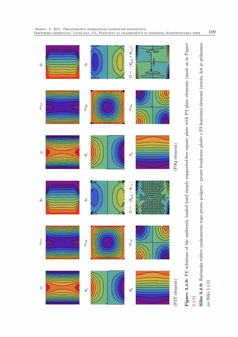
Bohinc, U. 2011. Prilagodljivo modeliranje ploskovnih konstrukcij
Doktorska disertacija. Ljubljana, UL, Fakulteta za gradbenistvo in geodezijo, Konstrukcijska smer 109
(P3T
elem
ent)
(P3Q
elem
ent)
Figure
3.4.9:FE
solution
sof
theuniformly
load
edhardsimply
supported-freesquareplate
withP3plate
elem
ents
(meshas
inFigure
3.4.8)
Slika3.4.9:Racunskaresiteven
akom
ernotogo
prostopodprte-prostekvadratneploscesP3koncn
imielem
enti(m
reza,kotje
prikazana
naSliki3.4.8)

110Bohinc, U. 2011. Adaptive modeling of plate structures
Doctoral thesis. Cachan, ENS Cachan, LMT
(Displacement w at center)
(Moment resultant mxx at center)
(Energy norm)
Figure 3.4.10: Comparison of the convergence of FE solutions for the uniformly loaded hard
simply supported-free square plate
Slika 3.4.10: Primerjava konvergence racunske resitve problema enakomerno togo prosto pod-
prte - proste kvadratne plosce

Bohinc, U. 2011. Prilagodljivo modeliranje ploskovnih konstrukcij
Doktorska disertacija. Ljubljana, UL, Fakulteta za gradbenistvo in geodezijo, Konstrukcijska smer 111
Figure 3.4.12: Reference solution of the uniformly loaded soft simply supported skew platewith legend also valid for Figures 3.4.14 and 3.4.13Slika 3.4.12: Referencna resitev enakomerno obremenjene mehko podprte romboidne ploscez legendo, ki velja tudi za Sliki 3.4.14 in 3.4.13

112Bohinc, U. 2011. Adaptive modeling of plate structures
Doctoral thesis. Cachan, ENS Cachan, LMT
(PIT element)
(PIQ element)
Figure 3.4.13: FE solution of the uniformly loaded soft simply supported skew plate with PIplate elementsSlika 3.4.13: Racunska resitev enakomerno obremenjene togo podprte romboidne plosce s PIkoncnimi elementi

Bohinc, U. 2011. Prilagodljivo modeliranje ploskovnih konstrukcij
Doktorska disertacija. Ljubljana, UL, Fakulteta za gradbenistvo in geodezijo, Konstrukcijska smer 113
(P3T element)
(P3Q element)
Figure 3.4.14: FE solution of the uniformly loaded soft simply supported skew plate with P3plate elements (mesh as in Figure 3.4.13)Slika 3.4.14: Racunska resitev enakomerno obremenjene togo podprte romboidne plosce s P3koncnimi elementi (mreza, kot je prikazana na Sliki 3.4.13)

114Bohinc, U. 2011. Adaptive modeling of plate structures
Doctoral thesis. Cachan, ENS Cachan, LMT
(Displacement w at center)
(Moment resultant mxx at center)
(Energy norm)
Figure 3.4.15: Comparison of the convergence of FE solutions for the uniformly loaded softsimply supported skew plateSlika 3.4.15: Primerjava konvergence racunske resitve problema enakomerno obremenjenemehko podprte romboidne plosce

Bohinc, U. 2011. Prilagodljivo modeliranje ploskovnih konstrukcij
Doktorska disertacija. Ljubljana, UL, Fakulteta za gradbenistvo in geodezijo, Konstrukcijska smer 115
Figure
3.4.17:Referen
cesolution
oftheuniformly
load
edsoft
simply
supportedL-shap
edplate
withlegendalso
validforFigures3.4.19
and3.4.18
Slika3.4.17:Referencn
aresiteven
akom
ernoob
remen
jenemeh
kopodprteLplosce
zlegendo,
kiveljatudiza
Sliki3.4.19
in3.4.18

116Bohinc, U. 2011. Adaptive modeling of plate structures
Doctoral thesis. Cachan, ENS Cachan, LMT
(PIT
element)
(PIQ
element)
Figure
3.4.18:FE
solution
oftheuniform
lyload
edsoft
simply
supported
L-sh
aped
plate
with
PIplate
elements
Slik
a3.4.18:Racu
nska
resiteven
akomern
oob
remen
jenemeh
kopodprte
Lplosce
sPIkon
cnim
ielem
enti

Bohinc, U. 2011. Prilagodljivo modeliranje ploskovnih konstrukcij
Doktorska disertacija. Ljubljana, UL, Fakulteta za gradbenistvo in geodezijo, Konstrukcijska smer 117
(P3T
elem
ent)
(P3Q
elem
ent)
Figure
3.4.19:
FE
solution
oftheuniformly
load
edsoft
simply
supportedL-shap
edplate
withP3plate
elem
ents
(meshas
inFigure
3.4.18)
Slika3.4.19:Racunskaresiteven
akom
ernoob
remen
jenemeh
kopodprteLploscesP3koncn
imielem
enti(m
reza,kotje
prikazananaSliki
3.4.18)

118Bohinc, U. 2011. Adaptive modeling of plate structures
Doctoral thesis. Cachan, ENS Cachan, LMT
(Displacement w at center)
(Moment resultant mxx at center)
(Energy norm)
Figure 3.4.20: Comparison of the convergence of FE solutions for the uniformly loaded softsimply supported L-shaped plateSlika 3.4.20: Primerjava konvergence racunske resitve problema enakomerno obremenjenemehko podprte L plosce

Bohinc, U. 2011. Prilagodljivo modeliranje ploskovnih konstrukcij
Doktorska disertacija. Ljubljana, UL, Fakulteta za gradbenistvo in geodezijo, Konstrukcijska smer 119
3.5 Chapter summary and conclusions
A Reissner/Mindlin plate theory, which covers the behavior of moderately thick plates
is presented. The Kirchhoff assumption is abandoned as the theory takes into account
the transverse shear: the midsurface deflection of the plate is independent of rotation of
normal fibers.
In the first section the basic equations are derived. The shear correction factor is
treated alongside for the sake of completeness. There are three coupled differential equa-
tions of sixth order for midsurface deflection w and two components of rotation φx, φy
which govern the deformation of the moderately thick plates. Since the hierarchic relation
of the Reissner/Mindlin theory to the Kirchhoff theory is followed throughout the deriva-
tion, one of the equations can be presented as the modified biharmonic equation. This
hierarchical treatment is advantageous since it enables us to clearly identify the novelties.
The Reissner/Mindlin theory is able to describe a larger set of boundary conditions.
There are three independent components of boundary traction loading: normal shear,
twisting and bending moment. However, being closer to the full three-dimensional theory,
and thus able to describe more flexible plate structures, the Reissner/Mindlin plates do
not handle concentrated loads - contrary to the Kirchhoff plates.
The introduction of transverse shear triggers some interesting phenomena. Most no-
table is the boundary layer effect, which concern the areas near the plate boundary, where
steep gradients of stress resultants exist. The influence of boundary layer effects is lim-
ited to the distance of the order of plate thickness into the plate interior. The existence
and strength of boundary layers is related to the type of boundary conditions imposed.
Maybe the most counter-intuitive fact concerning the boundary layers is, that it is the
most prominent along the free boundary of the plate. The singularities, already encoun-
tered in the Kirchhoff theory of thin plates, exist also in the Reissner/Mindlin theory.
The second section deals with the development of the finite element based on Reiss-
ner/Mindlin theory. An alternative notation enables the presentation of the finite elements
as the hierarchical extension of the DK thin plate elements. Additional degrees of free-
dom at the element mid-sides are directly related to the projection of the transverse shear
on the direction of the element side. An analysis of the stiffness matrix of the element
shows that the part related to the shear strain depends only on the mid-side degrees of
freedom. Equivalent formulation of triangular and quadrilateral elements is possible due
to the alternative element notation. A variation of the elements is also presented. Here

120Bohinc, U. 2011. Adaptive modeling of plate structures
Doctoral thesis. Cachan, ENS Cachan, LMT
the additional degrees of freedom are related to incompatible deformation modes, and are
thus subject to elimination by means of static condensation.
The chapter concludes with several typical plate problems, which illustrate the specific
issues of moderately thick plate modeling including singularities and boundary layers.
The performance of the presented finite elements is assessed in terms of the convergence
rates of various selected quantities. The functionality of element implementation is tested
through the comparison to the reference solutions. An interesting observation is made,
regarding the performance of the elements with the incompatible modes. Although the
elements are able to capture the transverse shear, they fail to detect the boundary layers.

Bohinc, U. 2011. Prilagodljivo modeliranje ploskovnih konstrukcij
Doktorska disertacija. Ljubljana, UL, Fakulteta za gradbenistvo in geodezijo, Konstrukcijska smer 121
Chapter 4
Thick plates: theory and finiteelement formulations
4.1 Introduction
A logical successor of the Reissner/Mindlin model in the hierarchy of the models for
bending of elastic isotropic plates is a higher-order plate model which includes through
the thickness stretching. The higher-order plate model, considered in this chapter is a
special case of a shell model presented in [Brank, 2005] and [Brank et al., 2008]. It treats
a plate as a 2d surface in a full 3d stress state. This is advantageous, since the usual
modification of 3d constitutive equations due to the plane stress assumption (see chapters
2 and 3) is omitted, resulting in a simpler implementation of complex material models for
example hiperelasticity or elasto-plasticity. Also the boundary layer effect, which is full
3d effect, is much better represented by the higher-order plate models as shown below.
The considered higher-order plate model fits between the Reisnner/Mindlin model and
the 3d solid model, which makes it an ideal choice for the model adaptivity of plates.
In this chapter we will thus present a new higher-order plate theory and a new higher-
order plate elements based on that theory. The elements will be a direct refinement of
the Reissner/Mindlin finite elements with cubic interpolation of displacement and linked
interpolation of displacement and rotations, denoted in previous chapter as P3T and P3Q.

122Bohinc, U. 2011. Adaptive modeling of plate structures
Doctoral thesis. Cachan, ENS Cachan, LMT
z
t
t = (1 + ε(0)zz )t −κzz(t/2)2
w
Figure 4.2.1: Kinematics of through-the-thickness deformation in the thick plate model
Slika 4.2.1: Kinematika deformacije vzdolz debeline plosce v modelu debelih plosc
4.2 Theory
We start by abandoning the assumption of zero through the thickness stress: σzz 6= 0. In
the case of 3d linear elasticity we thus have:
σzz = (λ+ 2µ)εzz + λ(εxx + εyy) 6= 0 (4.2.1)
with λ = νE(1+ν)(1−2ν)
, µ = E2(1+ν)
as Lame coefficients. Nevertheless in the limit t → 0 the
plane stress assumption σzz = 0 must be satisfied resulting in the thickness stretching εzz:
εzz = − λ
λ+ 2µ(εxx + εyy)
This kind of limit behavior can be achieved only if the strains εxx, εyy, εzz are of the same
order with respect to z coordinate. In such a case they can cancel each other in (4.2.1).
If for instance εxx, εyy are linear with respect to z coordinate, so must be εzz. The linear
variation of εzz with z also implies that the transverse displacement uz should be at least
quadratic function of z since εzz =∂uz
∂z.
4.2.1 Governing equations
Kinematic equations
The following kinematics of plate displacement is therefore assumed:
u = uRM + uS

Bohinc, U. 2011. Prilagodljivo modeliranje ploskovnih konstrukcij
Doktorska disertacija. Ljubljana, UL, Fakulteta za gradbenistvo in geodezijo, Konstrukcijska smer 123
where uRM denotes kinematics of Reissner/Mindlin model
uRM = wnΩ − zφ; nΩ = [0, 0, 1]T
and uS defines the displacements that produce the through-the-thickness stretch (see
Figure 4.2.1)
uS =((t/t− 1)z − κzzz
2/2)nΩ =
(ε(0)zz z − ε(1)zz z
2/t)nΩ (4.2.2)
The uS is a quadratic function of z coordinate; t is the thickness of the deformed plate,
t is the thickness of the plate prior to deformation, κzz = ε(1)zz 2/t is the parameter of the
stretch and nΩ the normal to the midsurface of the undeformed plate. The uS direction is
limited to the direction of nΩ. We denote the relative thickness change by ε(0)zz = t/t− 1.
The components of displacement w = [ux, uy, uz]T are:
ux = −zφx; uy = −zφy; uz = w + ε(0)zz z − ε(1)zz z2/t (4.2.3)
and the resulting strains are
εxx = −zκxx; 2εxy = −zκxy (4.2.4)
εyy = −zκyy ; 2εxz = γx + ε(0)zz,xz − ε(1)zz,xz2/t
εzz = ε(0)zz − 2zε(1)zz /t = ε(0)zz − zκzz; 2εyz = γy + ε(0)zz,yz − ε(1)zz,yz2/t
where the definitions from chapters 2 and 3 were employed
κxx = φx,x; γx = w,x − φx (4.2.5)
κyy = φy,y; γy = w,y − φy
κxy = φx,y + φy,x
Additionally, using the analogy with the deformation terms due to bending, which vary
with z, the curvature κzz was introduced in (4.2.4):
κzz = ε(1)zz /(t/2) (4.2.6)

124Bohinc, U. 2011. Adaptive modeling of plate structures
Doctoral thesis. Cachan, ENS Cachan, LMT
Constitutive equations
The Hooke’s relations for the 3d linear elastic material are:
σxx = (λ+ 2µ)εxx + λεyy + λεzz; σxy = 2µεxy (4.2.7)
σyy = (λ+ 2µ)εyy + λεxx + λεzz; σxz = 2µεxz
σzz = (λ+ 2µ)εzz + λεxx + λεyy; σyz = 2µεyz
Equilibrium equations
Equilibrium equations will be presented in the next section in their weak form.
4.2.2 Principle of virtual work
Virtual work of internal forces
The virtual work of internal forces that takes into account also kinematic and constitutive
equations, is defined by
δΠint(w,φ, ε(0)zz , κzz; δw, δφ, δε(0)zz , δκzz) =
∫
V
δεTσdΩ = (4.2.8)
∫
Ω
∫ t/2
−t/2
(σxxδεxx + σyyδεyy + σzzδεzz + σxy2δεxy + σxz2δεxz + σyz2δεyz) dzdΩ
where σ = [σxx, σyy, σzz, σxy, σxz, σyz]T are defined through (4.2.4), (4.2.5) and (4.2.7) in
terms of kinematic quantities and δε = [δεxx, δεyy, δεzz, 2δεxy, 2δεxz, 2δεyz]T are virtual
strains defined in terms of virtual kinematic quantities δw, δφ, δε(0)zz , δκzz in the same
manner as real strains are defined in terms of real kinematic quantities (4.2.4), (4.2.7).
mxx =
∫ t/2
−t/2
zσxxdz; myy =
∫ t/2
−t/2
zσyydz; mxy =
∫ t/2
−t/2
zσxydz (4.2.9)
qx =
∫ t/2
−t/2
σxzdz; qy =
∫ t/2
−t/2
σyzdz
mzz =
∫ t/2
−t/2
zσzzdz; nzz =
∫ t/2
−t/2
σzzdz (4.2.10)

Bohinc, U. 2011. Prilagodljivo modeliranje ploskovnih konstrukcij
Doktorska disertacija. Ljubljana, UL, Fakulteta za gradbenistvo in geodezijo, Konstrukcijska smer 125
After through the thickness integration of (4.2.8) and use of some algebraic manipulations,
we arrive at the following expression for the virtual work of internal forces:
δΠint =
∫
Ω
(δκTm+ δγT q + δε(0)zz nzz
)dΩ (4.2.11)
δΠint = δΠintκ + δΠint
γ + δΠintzz
δΠintκ =
∫
Ω
δκTm dΩ; δΠintγ =
∫
Ω
δγT q dΩ; δΠintzz =
∫
Ω
δε(0)zz nzz dΩ
where m = [mxx, myy, mxy, mzz]T and δκ = [δκxx, δκyy, δκxy, δκzz]
T . The vectors δγ and
δq represent virtual strains and shear forces respectively. Their definition will be given
below.
The components of m are related to the curvatures κ = [κxx, κyy, κxy, κzz]T through
(constitutive (4.2.14) and kinematic (4.2.4) equations are used in (4.2.9), (4.2.10))
mxx =t3
12((λ+ 2µ)κxx + λκyy + λκzz) (4.2.12)
myy =t3
12((λ+ 2µ)κyy + λκxx + λκzz)
mzz =t3
12((λ+ 2µ)κzz + λκxx + λκyy)
mxy =t3
12µκxy
and the stress resultant nzz is related to ε(0)zz through
nzz = t(λ + 2µ)ε(0)zz = CZε(0)zz ; CZ = t(λ+ 2µ) (4.2.13)
In matrix notation the constitutive matrix is
CB =t3
12
(λ+ 2µ) λ 0 λλ (λ+ 2µ) 0 λ0 0 µ 0λ λ 0 (λ+ 2µ)
(4.2.14)
which allows for the relations (4.2.12) to be expressed in a compact form:
m = CBκ (4.2.15)
In order to make the the theory more comparable to the Reissner/Mindlin one, we
decide to make the following decomposition of κzz:
κzz = κ(0)zz + κ(1)zz ; κ(0)zz = − λ
λ+ 2µ(κxx + κyy) =
−ν1− ν
(κxx + κyy) (4.2.16)

126Bohinc, U. 2011. Adaptive modeling of plate structures
Doctoral thesis. Cachan, ENS Cachan, LMT
Since we have
εzz = ε(0)zz − zκzz = ε(0)zz
−zκ(0)zz︷ ︸︸ ︷
− λ
λ + 2µ(εxx + εyy)−zκ(1)zz (4.2.17)
ε(1)zz = (t/2)κzz = (t/2)(κ(0)zz + κ(1)zz )
the decomposition leads to plane stress assumption σzz = 0, if ε(0)zz = 0 and κ
(1)zz = 0.
According to (4.2.3), the kinematics of stretch becomes:
uz = w + ε(0)zz z +1
2
ν
1− ν(κxx + κyy)z
2 − 1
2κ(1)zz z
2 (4.2.18)
By using (4.2.18), eq. (4.2.11) can be simplified to:
δΠintκ =
∫
Ω
δκTmdΩ =
∫
Ω
δκT CBκ dΩ = δΠint,RMκ + δΠint,∆
κ (4.2.19)
δΠint,RMκ =
∫
Ω
δκCBκ dΩ; δΠint,∆κ =
∫
Ω
δκ(1)zz CB,zzκ(1)zz dΩ
where κ = [κxx, κyy, κxy]T and CB is the constitutive matrix as defined in (2.2.13). Addi-
tionally, we have CB,zz =Et3(1−ν)
12(1+ν)(1−2ν)= D (1−ν)2
(1−2ν), where D = Et3
12(1−ν2).
Next, the expanded shear strain vector is introduced, see (4.2.4)
γ = [γx, γy, γ(1)x , γ(1)y , γ(2)x , γ(2)y ]T (4.2.20)
where
[2εxz, 2εyz]T = γ + zγ(1) +
z2
2γ(2); z = z/(t/2) (4.2.21)
[γx, γy]T = γ = ∇w − φ
[γ(1)x , γ(1)y ]T = γ(1) = (t/2)∇ε(0)zz
[γ(2)x , γ(2)y ]T = γ(2) = − (t/2)∇ε(1)zz
The components of the shear force vector q = [qx, qy, q(1)x , q
(1)y , q
(2)x , q
(2)y ]T are obtained from
(4.2.9) as:
q = cµt(γ + γ(2)/6
); q(1) = cµt
(γ(1)/3
); q(2) = cµt
(γ/6 + γ(2)/20
)(4.2.22)
where
σxz = c µ 2εxz; σyz = c µ 2εyz (4.2.23)
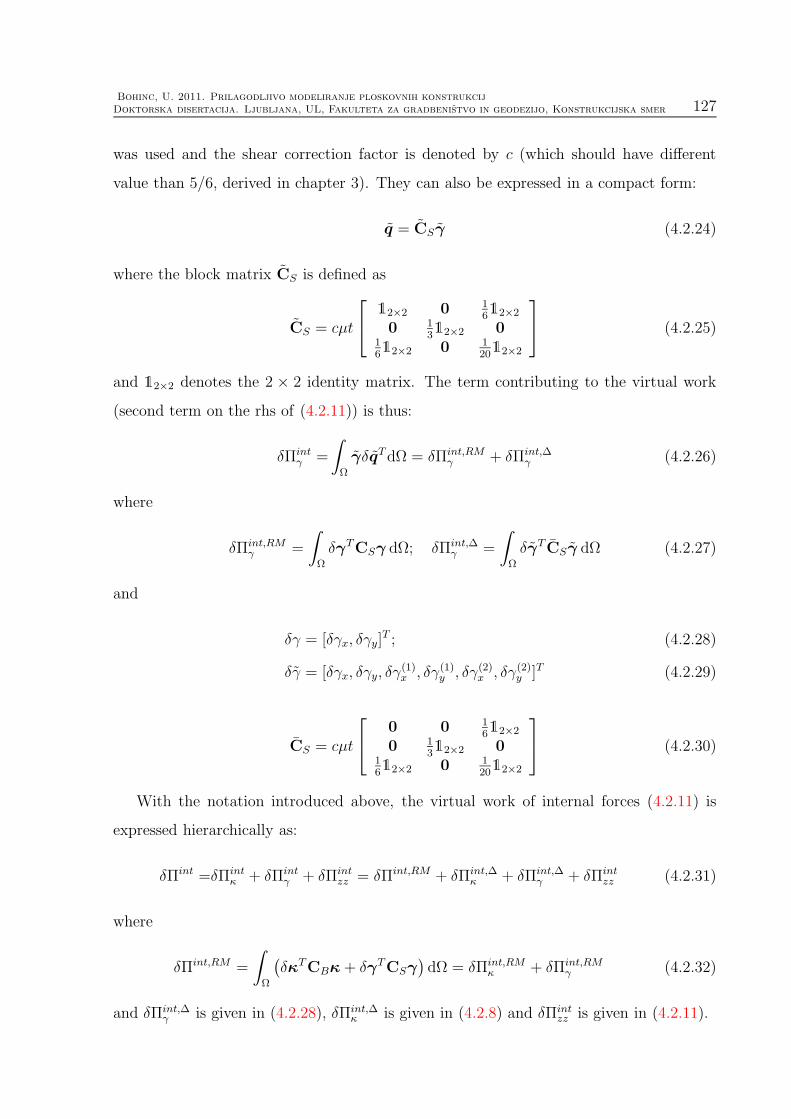
Bohinc, U. 2011. Prilagodljivo modeliranje ploskovnih konstrukcij
Doktorska disertacija. Ljubljana, UL, Fakulteta za gradbenistvo in geodezijo, Konstrukcijska smer 127
was used and the shear correction factor is denoted by c (which should have different
value than 5/6, derived in chapter 3). They can also be expressed in a compact form:
q = CSγ (4.2.24)
where the block matrix CS is defined as
CS = cµt
12×2 0 1612×2
0 1312×2 0
1612×2 0 1
2012×2
(4.2.25)
and 12×2 denotes the 2 × 2 identity matrix. The term contributing to the virtual work
(second term on the rhs of (4.2.11)) is thus:
δΠintγ =
∫
Ω
γδqTdΩ = δΠint,RMγ + δΠint,∆
γ (4.2.26)
where
δΠint,RMγ =
∫
Ω
δγTCSγ dΩ; δΠint,∆γ =
∫
Ω
δγT CSγ dΩ (4.2.27)
and
δγ = [δγx, δγy]T ; (4.2.28)
δγ = [δγx, δγy, δγ(1)x , δγ(1)y , δγ(2)x , δγ(2)y ]T (4.2.29)
CS = cµt
0 0 1612×2
0 1312×2 0
1612×2 0 1
2012×2
(4.2.30)
With the notation introduced above, the virtual work of internal forces (4.2.11) is
expressed hierarchically as:
δΠint =δΠintκ + δΠint
γ + δΠintzz = δΠint,RM + δΠint,∆
κ + δΠint,∆γ + δΠint
zz (4.2.31)
where
δΠint,RM =
∫
Ω
(δκTCBκ+ δγTCSγ
)dΩ = δΠint,RM
κ + δΠint,RMγ (4.2.32)
and δΠint,∆γ is given in (4.2.28), δΠint,∆
κ is given in (4.2.8) and δΠintzz is given in (4.2.11).
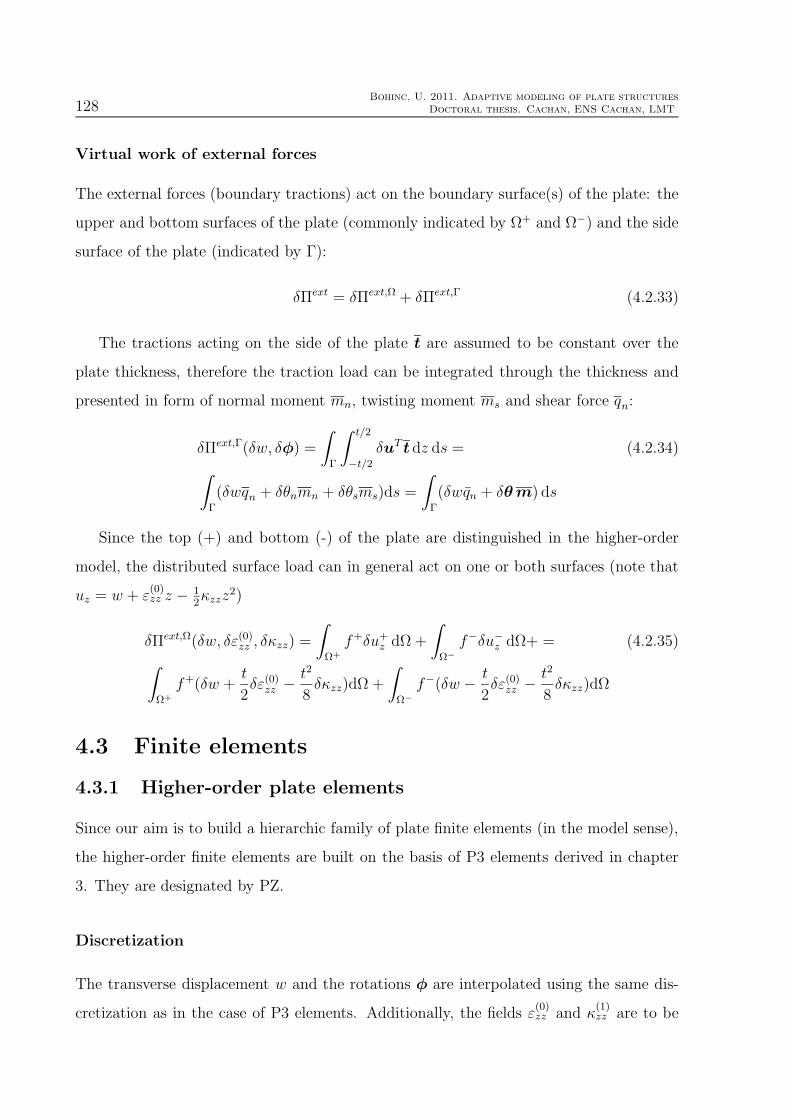
128Bohinc, U. 2011. Adaptive modeling of plate structures
Doctoral thesis. Cachan, ENS Cachan, LMT
Virtual work of external forces
The external forces (boundary tractions) act on the boundary surface(s) of the plate: the
upper and bottom surfaces of the plate (commonly indicated by Ω+ and Ω−) and the side
surface of the plate (indicated by Γ):
δΠext = δΠext,Ω + δΠext,Γ (4.2.33)
The tractions acting on the side of the plate t are assumed to be constant over the
plate thickness, therefore the traction load can be integrated through the thickness and
presented in form of normal moment mn, twisting moment ms and shear force qn:
δΠext,Γ(δw, δφ) =
∫
Γ
∫ t/2
−t/2
δuT tdz ds = (4.2.34)
∫
Γ
(δwqn + δθnmn + δθsms)ds =
∫
Γ
(δwqn + δθm) ds
Since the top (+) and bottom (-) of the plate are distinguished in the higher-order
model, the distributed surface load can in general act on one or both surfaces (note that
uz = w + ε(0)zz z − 1
2κzzz
2)
δΠext,Ω(δw, δε(0)zz , δκzz) =
∫
Ω+
f+δu+z dΩ +
∫
Ω−
f−δu−z dΩ+ = (4.2.35)
∫
Ω+
f+(δw +t
2δε(0)zz − t2
8δκzz)dΩ +
∫
Ω−
f−(δw − t
2δε(0)zz − t2
8δκzz)dΩ
4.3 Finite elements
4.3.1 Higher-order plate elements
Since our aim is to build a hierarchic family of plate finite elements (in the model sense),
the higher-order finite elements are built on the basis of P3 elements derived in chapter
3. They are designated by PZ.
Discretization
The transverse displacement w and the rotations φ are interpolated using the same dis-
cretization as in the case of P3 elements. Additionally, the fields ε(0)zz and κ
(1)zz are to be

Bohinc, U. 2011. Prilagodljivo modeliranje ploskovnih konstrukcij
Doktorska disertacija. Ljubljana, UL, Fakulteta za gradbenistvo in geodezijo, Konstrukcijska smer 129
discretized. A bilinear discretization of both fields is assumed:
ε(0)zz,h =
∑
I
NI ε(0)zz,I; κ
(1)zz,h =
∑
I
NI κ(1)zz,I (4.3.1)
where ε(0)zz,I and κ
(1)zz,I are the additional nodal degrees of freedom. The vertex degrees
of freedom of the PZ element are thus uI = [wI , θx,I , θy,I , ε(0)zz,I, κ
(1)zz,I ]
T and the midside
degrees of freedom are uIJ = [γIJ ]. The elements have nen vertex nodes and nen midside
nodes (nen=4 for the quadrilateral, and nen = 3 for triangular elements). The vertex
nodes are numbered as I = 1, . . . , nen, the midside nodes as IJ = (nen + 1), . . . , 2nen.
Element degrees of freedom are arranged into u = [uT1 , · · · , uT
nen, uTnen+1, · · · , uT
2nen]T .
The interpolations can be expressed as:
κh =∑
I
Bκ,IuI +∑
IJ
Bκ,IJuIJ ; γh =∑
IJ
Bγ,IJ uIJ ; (4.3.2)
ε(0)zz,h =
∑
I
Bε(0)zz ,I
uI ; γ(1)h =
∑
I
Bγ(1),IuI ;
κ(1)zz,h =
∑
I
Bκ(1)zz ,I
uI ; γ(2)h =
∑
I
Bγ(2),IuI +∑
IJ
Bγ(2),IJ uIJ
where
κh = [κxx,h, κyy,h, κxy,h]T ; γh = [γx,h, γy,h]
T
γ(1)h =
t
2
[∂ε
(0)zz,h
∂x,∂ε
(0)zz,h
∂y
]T; γ
(2)h =
t
2
[∂ε
(1)zz,h
∂x,∂ε
(1)zz,h
∂y
]T(4.3.3)

130Bohinc, U. 2011. Adaptive modeling of plate structures
Doctoral thesis. Cachan, ENS Cachan, LMT
The following definitions apply:
Bκ,I = [Bκxx,I ,Bκyy,I ,Bκxy,I ]T = [BP3
κ,I , 03×2]; (4.3.4)
Bκ,IJ = BP3κ,IJ ; Bγ,IJ = BP3
γ,IJ
Bκ(1)zz ,I
= [0, 0, 0, 0, NI]; Bε(0)zz ,I
= [0, 0, 0, NI , 0]
Bγ(1),I = (t/2)
[0 0 0 NI,x 00 0 0 NI,y 0
]
Bγ(2),I = B(0)
γ(2),I+B
(1)
γ(2),I
B(0)
γ(2),I= − ν
1 − ν(t/2)2
[∂∂x(Bκxx,I +Bκyy,I)
∂∂y(Bκxx,I +Bκyy,I)
]
B(1)
γ(2),I= −(t/2)2
[0 0 0 0 NI,x
0 0 0 0 NI,y
]
Bγ(2),IJ = − ν
1 − ν(t/2)2
[∂∂x(Bκxx,IJ +Bκyy,IJ)
∂∂y(Bκxx,IJ +Bκyy,IJ)
]
Stiffness matrix
The stiffness matrixK of PZ element is obtained by inserting the discretization (4.3.2) into
(4.2.11) and taking into account the constitutive relations (4.2.13), (4.2.15) and (4.2.24).
It consists of three parts, which correspond to bending stiffness, shear stiffness and the
through-the-thickness stretching stiffness:
K = KB +KS +KZ (4.3.5)
The stiffness matrix is expressed as a block matrix K = [Kij], where blocks Kij
correspond to the interaction of degrees of freedom of nodes i and j. The stiffness matrix
is expressed as a block matrix K = [Kij ], where blocks Kij correspond to the interaction
of degrees of freedom of nodes i and j. The indexes referring to the vertex node are
denoted by I and J . The indexes IJ and KL are used to denote the midside nodes. The
stiffness matrix is then organized as:
K =
[[KI,J ] [KI,KL]
[KIJ,J ] [KIJ,KL]
](4.3.6)

Bohinc, U. 2011. Prilagodljivo modeliranje ploskovnih konstrukcij
Doktorska disertacija. Ljubljana, UL, Fakulteta za gradbenistvo in geodezijo, Konstrukcijska smer 131
According to the (4.2.19), the bending stiffness KBij is a sum of two components
KBij = KB,0
ij +KB,∆ij
where
KB,0ij =
∫
Ω
BTκ,iCBBκ,j dΩ; KB,∆
ij =
∫
Ω
BT
κ(1)zz ,i
CB,zzBκ(1)zz ,j
dΩ (4.3.7)
Notice that, since Bκ,I = [BP3κ,I , 03×2], the matrixKB,0
I,J corresponds to the bending stiffness
matrix of P3 elements.
KB,0I,J =
∫
Ωe
BTκ,ICBBκ,JdΩ =
[KB,P3
I,J 03×2
02×3 02×2
](4.3.8)
Since the interpolation of κ(1)zz is independent of all degrees of freedom other than κ
(1)zz,i,
the deformation mode κ(1)zz is independent of bending. The block matrix KB,∆
I,J is thus:
KB,∆I,J =
[04×4 04×1
01×4 Kκ(1)zz ,I,J
](4.3.9)
where
Kκ(1)zz ,I,J
=
∫
Ω
BT
κ(1)zz ,I
CB,zzBκ(1)zz ,J
dΩ =
∫
Ω
CB,zzNINJdΩ (4.3.10)
Similarly, from (4.2.26), (4.2.27), we can decompose the shear part of the stiffness
matrix into
KS = KS,0 +KS,∆
where (according to (4.2.26), (4.3.2))
KS,0ij =
∫
Ω
BTγ,iCSBγ,j dΩ (4.3.11)
and
KS,∆ij =
1
3
∫
Ω
BTγ(1),iCSBγ(1),j dΩ +
1
20
∫
Ω
BTγ(2),iCSBγ(2),j dΩ+
1
6
∫
Ω
BTγ,iCSBγ(2),j dΩ +
1
6
∫
Ω
BTγ(2),iCSBγ,j dΩ
The part KS,∆ij corresponds to the contribution of the through the thickness stretching to
the shear deformation.

132Bohinc, U. 2011. Adaptive modeling of plate structures
Doctoral thesis. Cachan, ENS Cachan, LMT
Notice, that the block matrix KS,0IJ,KL corresponds to the shear stiffness matrix of P3
elements (4.3.2)
KS,0IJ,KL =
∫
Ωe
BTγ,IJCSBγ,KLdΩ =
∫
Ωe
BP3,Tγ,IJ CSB
P3γ,KLdΩ = KS,P3
IJ,KL (4.3.12)
and
KS,0I,J = 05×5; KS,0
I,KL = 05×1; KS,0IJ,J = 01×5
The part of the stiffness matrix, which directly corresponds to the through the thick-
ness stretching KZ is a block matrix
KZI,J =
∫
Ω
BT
ε(0)zz ,I
CZBε(0)zz ,J
dΩ; KZIJ,J = 01×5; KZ
I,KL = 05×1; KZIJ,KL = 01×1
Load vector
x
y
z
Ω+
Ω−
Γ
Figure 4.3.1: Designation of plate surfaces Ω+, Ω− and Γ
Slika 4.3.1: Oznaka povrsin Ω+, Ω− in Γ
The load vector f is revealed by inserting the discretization (4.3.2) into (4.2.34) and
(4.2.35). Since we distinguish between the top and bottom surface (see Figure 4.3.1) Ω+
and Ω−, the load vector consists of three parts f = ff+ + ff− + ft, where
ff± =
∫
Ωe
f± (Bw ± t
2B
ε(0)zz
+t2
8Bκzz
)dΩ; (4.3.13)
ft =
∫
ΓNe
(qBw +mTBθ) ds
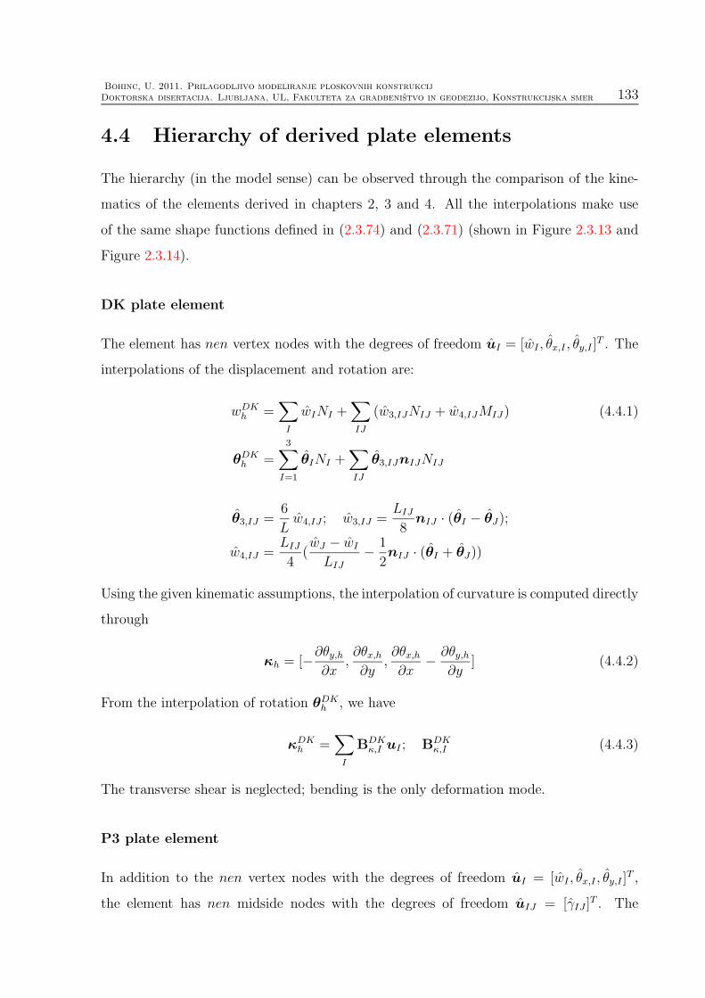
Bohinc, U. 2011. Prilagodljivo modeliranje ploskovnih konstrukcij
Doktorska disertacija. Ljubljana, UL, Fakulteta za gradbenistvo in geodezijo, Konstrukcijska smer 133
4.4 Hierarchy of derived plate elements
The hierarchy (in the model sense) can be observed through the comparison of the kine-
matics of the elements derived in chapters 2, 3 and 4. All the interpolations make use
of the same shape functions defined in (2.3.74) and (2.3.71) (shown in Figure 2.3.13 and
Figure 2.3.14).
DK plate element
The element has nen vertex nodes with the degrees of freedom uI = [wI , θx,I , θy,I ]T . The
interpolations of the displacement and rotation are:
wDKh =
∑
I
wINI +∑
IJ
(w3,IJNIJ + w4,IJMIJ ) (4.4.1)
θDKh =
3∑
I=1
θINI +∑
IJ
θ3,IJnIJNIJ
θ3,IJ =6
Lw4,IJ ; w3,IJ =
LIJ
8nIJ · (θI − θJ);
w4,IJ =LIJ
4(wJ − wI
LIJ− 1
2nIJ · (θI + θJ))
Using the given kinematic assumptions, the interpolation of curvature is computed directly
through
κh = [−∂θy,h∂x
,∂θx,h∂y
,∂θx,h∂x
− ∂θy,h∂y
] (4.4.2)
From the interpolation of rotation θDKh , we have
κDKh =
∑
I
BDKκ,I uI ; BDK
κ,I (4.4.3)
The transverse shear is neglected; bending is the only deformation mode.
P3 plate element
In addition to the nen vertex nodes with the degrees of freedom uI = [wI , θx,I , θy,I ]T ,
the element has nen midside nodes with the degrees of freedom uIJ = [γIJ ]T . The

134Bohinc, U. 2011. Adaptive modeling of plate structures
Doctoral thesis. Cachan, ENS Cachan, LMT
interpolations are
wP3h = wDK
h −∑
IJ
1
4LIJ γIJMIJ ; (4.4.4)
θP3h = θDK
h +∑
IJ
3
2nIJ γIJNIJ
The curvature interpolation κP3h is defined by the rotation θP3
h
κP3h = κDK
h + κh; κh =∑
IJ
Bκ,IJuIJ ; Bκ,IJ (4.4.5)
The interpolation of the transverse shear is:
γP3h =
∑
I
NI γh,I (4.4.6)
where the nodal values γh,I depend on the midside degrees of freedom γIJ according to
γh,I =γIKnIJ − γIJnIK
nIJ · sIK(4.4.7)
Note, that the interpolation of the transverse shear conform to the assumed kinematics
only along the sides of the element. At the element interior, an assumption of the variation
of the transverse shear strain is made.
PZ plate element
Element has nen vertex nodes with the degrees of freedom uI = [wI , θx,I , θy,I , ε(0)zz,I, κ
(1)zz,I ]
T ,
and nen midside nodes with the degrees of freedom uIJ = [γIJ ]T . The kinematics of the
material point is interpolated as
uPZh = uP3
h + uSh (4.4.8)
uP3h = wP3
h nΩ − zφP3h ; uS
h =(ε(0)zz z − ε(1)zz z
2/t)nΩ
nΩ = [0, 0, 1]T ; φP3h = [φP3
x,h, φP3y,h]
T = [−θP3y,h,+θ
P3x,h]
T
The curvature interpolation corresponds to the curvature interpolation of P3 element:
κPZh = κP3
h (4.4.9)

Bohinc, U. 2011. Prilagodljivo modeliranje ploskovnih konstrukcij
Doktorska disertacija. Ljubljana, UL, Fakulteta za gradbenistvo in geodezijo, Konstrukcijska smer 135
The transverse shear is interpolated as
γPZh = γP3
h + zγ(1)h +
z2
2γ(2)h ; z =
z
t/2(4.4.10)
γ(1)h =
∑
I
Bγ(1),I uI ;
γ(2)h =
∑
I
Bγ(2),I uI +
∑
IJ
Bγ(2),IJ uIJ
The matrices Bγ(1),I , Bγ(2),I and B
γ(2),IJ are defined in (4.3.4).
The discretizations of hrough the thickness deformation ε(0)zz,h and κ
(1)zz,h are defined by
(4.3.1):
ε(0)zz,h =
∑
I
NI ε(0)zz,I; κ
(1)zz,h =
∑
I
NI κ(1)zz,I (4.4.11)

136Bohinc, U. 2011. Adaptive modeling of plate structures
Doctoral thesis. Cachan, ENS Cachan, LMT
4.5 Examples
The selected problems are solved with the PZQ and PZT finite elements. Due to its
hierarchical construction, the basic novelty of the solution, compared to those obtained
with P3Q or P3T elements, can be described with fields ε(0)zz and κzz. Both components
have the strongest impact on the stress component σzz which varies through the thickness
as
σzz(z) = (λ+ 2µ)(ε(0)zz − zκzz) + λεxx + λεyy
In the following, the quantities σ+zz = σzz(t/2) and ∆σzz = (λ+ 2µ)κzz will be presented.
Since in the following problems, the loading is applied on the top surface Ω+, the value
of σ+zz corresponds to the loading f . The quantity ∆σzz can be interpreted as the shift of
midsurface relative to the surfaces Ω+ and Ω− (see Figure 4.2.1).
4.5.1 Uniformly loaded simply supported square plate
The square plate of side length a = 10 and thickness t = 1 under uniform loading f = 1
is analyzed. The sides of the plate at x = 0, a are hard simply supported, while the sides
at y = 0, a are soft simply supported. The material is linear elastic and isotropic, with
Young’s modulus E = 10.92× 10⁴ and Poisson’s ratio ν = 0.3. The problem is identical
to that analyzed already in section 3.4.1.
a
a
E,ν,t,f
Figure 4.5.1: Problem definition and geometry for the uniformly loaded hard-soft simplysupported square plate (t/a=1/10)Slika 4.5.1: Definicija in geometrija problema enakomerno obremenjene togor-mehko prostopodprte plosce (t/a=1/10)

Bohinc, U. 2011. Prilagodljivo modeliranje ploskovnih konstrukcij
Doktorska disertacija. Ljubljana, UL, Fakulteta za gradbenistvo in geodezijo, Konstrukcijska smer 137
Finite element solutions on a regular mesh are shown in Figure 4.5.2. When compared
to the solutions obtained with PQ3 and PT3 elements (see Figure 3.4.4) one notices,
that the basic features of the PZQ/PZT solutions are captured qualitatively at the same
level. The major difference is in the stress component σzz. The interpolation field ∆σzz
indicates the shift of the position the midsurface relative to the plate surfaces.
4.5.2 Uniformly loaded soft simply supported L-shaped plate
Uniformly loaded soft simply supported L-shaped plate with the geometry shown in Figure
4.5.4 is analyzed. The side length is a = 10 and thickness of the plate t = 1. The material
is linear elastic and isotropic, with Young’s modulus E = 10.92× 10⁴ and Poisson’s ratio
ν = 0.3. The problem is identical to that presented in section 3.4.4.
a
a/2
a
a/2
E,ν,t,f
Figure 4.5.4: Problem definition and geometry for the uniformly loaded soft simply supportedL shaped plate (t/a=1/10)Slika 4.5.4: Definicija in geometrija problema enakomerno obremenjene mehko podprte L plosce(t/a=1/10)
The finite element solution on a regular mesh is shown in Figure 4.5.5. The solution
captures both the singularity at the re-entrant corner as well as the boundary layers along
the supports. In that sense, the solution is close to the solution obtained with the P3
elements (see Figure 3.4.19). However, the ability of PZ elements to take into account also
the through-the-thickness stretching is manifested in the nonzero values of ∆σzz. Notice,
that the singularity at the re-entrant corner, while it significantly affects the moments
and shear forces, it does not have a significant effect on ∆σzz. In the interior of the plate,
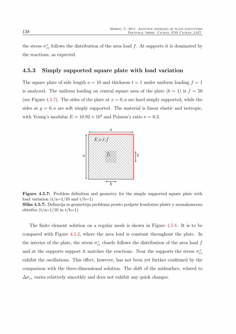
138Bohinc, U. 2011. Adaptive modeling of plate structures
Doctoral thesis. Cachan, ENS Cachan, LMT
the stress σ+zz follows the distribution of the area load f . At supports it is dominated by
the reactions, as expected.
4.5.3 Simply supported square plate with load variation
The square plate of side length a = 10 and thickness t = 1 under uniform loading f = 1
is analyzed. The uniform loading on central square area of the plate (b = 1) is f = 50
(see Figure 4.5.7). The sides of the plate at x = 0, a are hard simply supported, while the
sides at y = 0, a are soft simply supported. The material is linear elastic and isotropic,
with Young’s modulus E = 10.92× 10⁴ and Poisson’s ratio ν = 0.3.
a
a
b
b
f1
E,ν,t,f
Figure 4.5.7: Problem definition and geometry for the simply supported square plate withload variation (t/a=1/10 and t/b=1)Slika 4.5.7: Definicija in geometrija problema prosto podprte kvadratne plosce y neenakomernoobtezbo (t/a=1/10 in t/b=1)
The finite element solution on a regular mesh is shown in Figure 4.5.8. It is to be
compared with Figure 4.5.2, where the area load is constant throughout the plate. In
the interior of the plate, the stress σ+zz closely follows the distribution of the area load f
and at the supports support it matches the reactions. Near the supports the stress σ+zz
exhibit the oscillations. This effect, however, has not been yet further confirmed by the
comparison with the three-dimensional solution. The shift of the midsurface, related to
∆σzz varies relatively smoothly and does not exhibit any quick changes.

Bohinc, U. 2011. Prilagodljivo modeliranje ploskovnih konstrukcij
Doktorska disertacija. Ljubljana, UL, Fakulteta za gradbenistvo in geodezijo, Konstrukcijska smer 139
(PZT element)
(PZQ element)
Figure 4.5.2: FE solution of the uniformly loaded simply supported square plate with PZ plate
elements
Slika 4.5.2: Racunska resitev enakomerno obremenjene prosto podprte kvadratne plosce s PZ
koncnimi elementi

140Bohinc, U. 2011. Adaptive modeling of plate structures
Doctoral thesis. Cachan, ENS Cachan, LMT
Figure 4.5.3: Legend for Figures 4.5.2Slika 4.5.3: Legenda za Slike 4.5.2

Bohinc, U. 2011. Prilagodljivo modeliranje ploskovnih konstrukcij
Doktorska disertacija. Ljubljana, UL, Fakulteta za gradbenistvo in geodezijo, Konstrukcijska smer 141
(PZT element)
(PZQ element)
Figure 4.5.5: FE solution of the uniformly loaded soft simply supported L shaped plate withPZ plate elementsSlika 4.5.5: Racunska resitev enakomerno obremenjene mehko podprte L plosce s PZ koncnimielementi

142Bohinc, U. 2011. Adaptive modeling of plate structures
Doctoral thesis. Cachan, ENS Cachan, LMT
Figure 4.5.6: Legend for Figures 4.5.5Slika 4.5.6: Legenda za Slike 4.5.5

Bohinc, U. 2011. Prilagodljivo modeliranje ploskovnih konstrukcij
Doktorska disertacija. Ljubljana, UL, Fakulteta za gradbenistvo in geodezijo, Konstrukcijska smer 143
(PZT element)
(PZQ element)
Figure 4.5.8: FE solution of the simply supported square plate with load variation with PZ
plate elements
Slika 4.5.8: Racunska resitev prosto podprte kvadratne plosce y neenakomerno obtezbo s PZ
koncnimi elementi

144Bohinc, U. 2011. Adaptive modeling of plate structures
Doctoral thesis. Cachan, ENS Cachan, LMT
Figure 4.5.9: Legend for Figures 4.5.8Slika 4.5.9: Legenda za Slike 4.5.8

Bohinc, U. 2011. Prilagodljivo modeliranje ploskovnih konstrukcij
Doktorska disertacija. Ljubljana, UL, Fakulteta za gradbenistvo in geodezijo, Konstrukcijska smer 145
4.6 Chapter summary and conclusions
Both Kirchhoff and Reissner/Mindlin theories neglect the normal stress σzz. The normal
stress is significant in the regions near the supports, point loads and at sharp changes
of plate thickness. In this chapter a higher-order plate theory is presented, which takes
explicitly into account also the through the thickness stretching and consequently σzz is
not neglected. No assumptions are made regarding the stress state which enables the use
of full three dimensional constitutive relations.
Assumed kinematics of the plate deformation allows for the linear variation of the nor-
mal strain through the thickness of the plate. Consistent derivation of the two-dimensional
principle of virtual work is presented in the following. Owing to the chosen interpolation
of the normal strain it is possible to follow hierarchical relations to the Reissner/Mindlin
model and the differences of both theories are clearly visible. A concise treatment of the
computation of terms involved in principle of virtual work is given.
Based on the proposed theory, a novel finite element is developed. Since the theory
is formulated as the hierarchical extension of the Reissner/Mindlin theory, so is the for-
mulation of the proposed finite element based on the P3 elements. Two additional nodal
degrees of freedom are introduced. They can be directly related to the constant and lin-
ear variation of normal stress σzz. The loading on top and bottom of the plate is treated
separately.
The chapter concludes with several numerical tests. Since the full three-dimensional
solution is unavailable and due to the hierarchical nature of the elements, the solution is
rather compared to solution obtained with P3 elements. The results of the computations
confirm the functionality of the finite element implementation. Numerical tests show that
the significant normal strain is limited to the relative narrow area close to the supports.
Additionally, small oscillations of the normal strain are observed near the supports.

146Bohinc, U. 2011. Adaptive modeling of plate structures
Doctoral thesis. Cachan, ENS Cachan, LMT

Bohinc, U. 2011. Prilagodljivo modeliranje ploskovnih konstrukcij
Doktorska disertacija. Ljubljana, UL, Fakulteta za gradbenistvo in geodezijo, Konstrukcijska smer 147
Chapter 5
Discretization error estimates
5.1 Introduction. Classification of error estimates
Finite element method is a numerical method, which gives only an approximate solution
to a given boundary value problem ([Zienkiewicz Taylor, 2000], [Ibrahimbegovic, 2009]).
It is therefore natural to try to evaluate the error of the approximate solution with respect
to the (unknown) exact solution. The main reason to deal with a measure of how close
the finite element approximation uh is to the exact solution u is the quality control of the
approximate solution and the adaptivity of the finite element mesh related to adaptive
modeling of disretization problem (e.g. see [Ainsworth Oden, 2000], [Ladeveze Pelle,
2006], [Stein Ramm, 2003]). Quality control is needed in order to meet a predefined limit
of error of approximation, which will guarantee a desired quality of the approximate solu-
tion. If the guarantee that the error remains inside the error bounds has to be provided,
we will seek for error estimates, which can be obtained by a rigorous mathematical anal-
ysis. Although the true error bounds can be very attractive, they are often compromised
by the fact that these estimates are very pessimistic and can overestimate the error by
several orders of magnitude.
A pretty good idea of overall quality of approximation can also be obtained by error
indicators ([Babuska Rheinboldt, 1978]), which do not provide error bounds. However,
error indicators are not only easier to handle but also represent the actual error better
than the error estimates do. Error indicators can thus provide efficient and also reliable
basis for adaptive modeling of the finite element mesh. In other words, they can be
effectively used to steer the adaptive algorithms in order to get optimal accuracy of a
finite element analysis with a minimum number of degrees of freedom. In what follows,
we will refer mainly to error indicators. Moreover, we will not strictly distinguish between

148Bohinc, U. 2011. Adaptive modeling of plate structures
Doctoral thesis. Cachan, ENS Cachan, LMT
error estimates and error indicators. In what follows, the word estimate will denote either
estimate or indicator.
Yet another classification of error estimates concerns a priori versus a posteriori error
estimates. The a priori error estimates consider the asymptotic behavior of the error with
respect to the element size h and the order p of the polynomial approximation. They do
not provide the information on the actual error of the finite element approximation uh.
The a posteriori error estimates rely on postprocessing of the finite element approximation
uh to obtain the error estimates of the finite element approximation uh. There are
basically two distinct types of a posteriori error estimates: recovery based error estimates
and residual based error estimates.
Recovery based error estimates are much more popular than the residual based error
estimates, since they provide easier way for the assessment of the finite element approx-
imation error. The Superconvergent patch recovery (SPR) rely on the existence of the
superconvergent points, where the rate of the convergence of gradient of the finite ele-
ment solution is higher than elsewhere in the element. The recovered (i.e. smoother)
gradient of the solution can be constructed over the whole domain based on the values at
superconvergent points. The recovered gradient of this kind can serve as an approxima-
tion of the gradient of the exact solution. The error is usually estimated by evaluating
the energy norm of the difference between the finite element solution and the recovered
approximation of the exact solution.
Residual based error estimates make use of the residuals of the finite element approx-
imation, either explicitly or implicitly ([Ainsworth Oden, 2000], [Ladeveze Pelle, 2006],
[Ladeveze Leguillon, 1983], [Stein Ramm, 2003], [Becher Rannacher, 2001]). Explicit
residual based error estimates rely on a direct computation of the interior element resid-
uals and the jumps at the element boundaries to find an estimate for the error ([Babuska
Rheinboldt, 1978], [Babuska Miller, 1987]). Implicit residual based error estimates involve
construction of auxiliary boundary value problems, whose solution yields an approxima-
tion of the actual error. The auxiliary boundary value problems that need to be solved
are local in a sense that they are posed on either patch of elements (subdomain residual
method) or on single element (element residual method (EqR), e.g. see [Stein Ramm,
2003]). We note that the element residual method needs to approximate the prescribed
Neumann boundary conditions on each single element.
The above mentioned error estimate methods are all concerned with the global energy
norm of the error. In the finite element analysis it is, however, frequently the case that

Bohinc, U. 2011. Prilagodljivo modeliranje ploskovnih konstrukcij
Doktorska disertacija. Ljubljana, UL, Fakulteta za gradbenistvo in geodezijo, Konstrukcijska smer 149
a specific output data (i.e. a stress at the selected point) is of special interest. The
goal-oriented error estimates were developed for such cases. They estimate the error in
individual quantity of interest by using duality techniques [Ainsworth Oden, 2000]. The
key for estimating the error in such quantity is the formulation of an auxiliary problem,
which is the dual problem to the primal actually considered. The dual problem filters out
the necessary information for an accurate estimate of the error in the quantity of interest.
The estimates of this kind, however, will not be considered in this work.
A posteriori error estimates/indicators
Recovery Based Residual Based Goal oriented
Superconvergent patch recovery (SPR)Lumped projection Implicit Explicit
Subdomain residual method Element residual method
Equilibrated residual method (EqR)
Figure 5.1.1: Rough classification of a-posteriori error estimates/indicators
Slika 5.1.1: Groba klasifikacija a-posteriori ocen napake
The above introduced classification of error estimates/indicators is presented in Figure
5.1.1. For more refined classification see e.g. [Ainsworth Oden, 2000].
5.2 Definitions. Linear elasticity as a model problem
In order to clarify the notation, we further study a model problem of linear elasticity. The
weak formulation of the problem is written as:
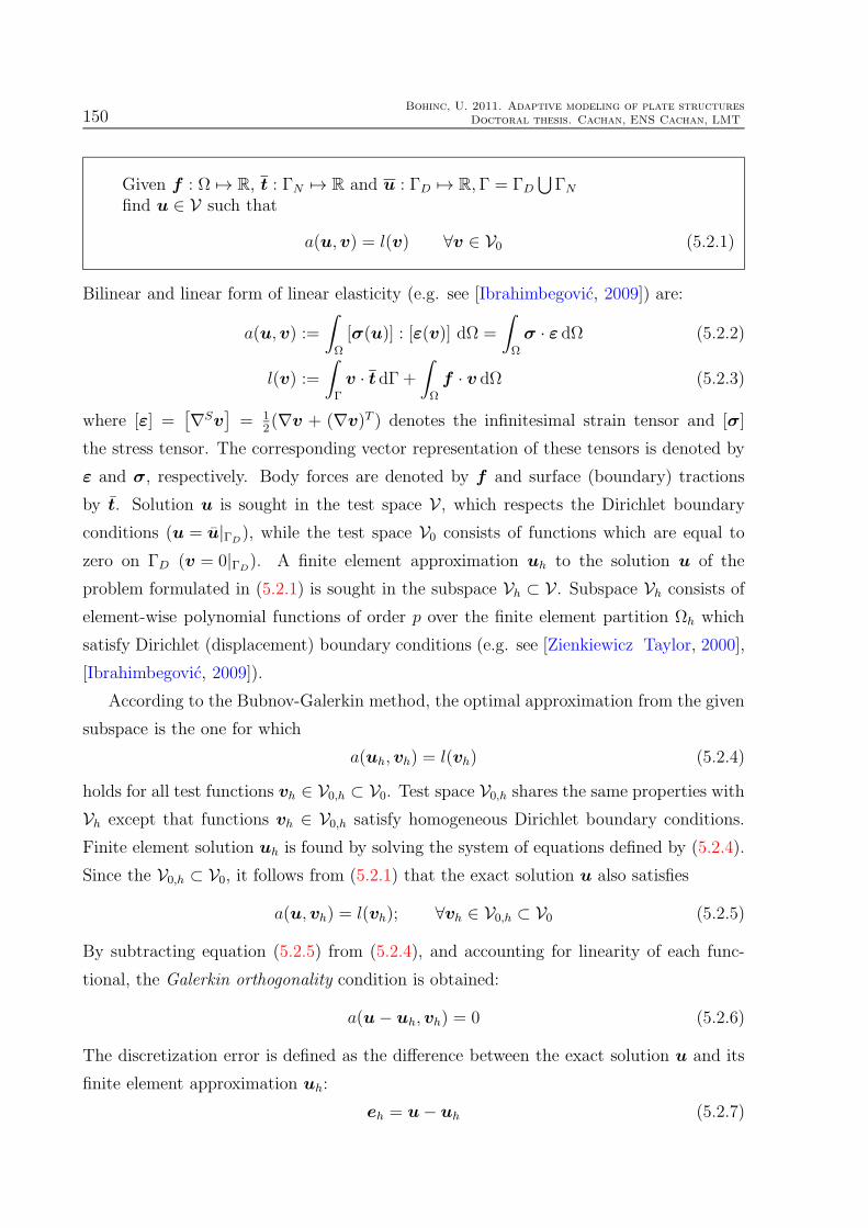
150Bohinc, U. 2011. Adaptive modeling of plate structures
Doctoral thesis. Cachan, ENS Cachan, LMT
Given f : Ω 7→ R, t : ΓN 7→ R and u : ΓD 7→ R,Γ = ΓD
⋃ΓN
find u ∈ V such that
a(u, v) = l(v) ∀v ∈ V0 (5.2.1)
Bilinear and linear form of linear elasticity (e.g. see [Ibrahimbegovic, 2009]) are:
a(u, v) :=
∫
Ω
[σ(u)] : [ε(v)] dΩ =
∫
Ω
σ · ε dΩ (5.2.2)
l(v) :=
∫
Γ
v · t dΓ +
∫
Ω
f · v dΩ (5.2.3)
where [ε] =[∇Sv
]= 1
2(∇v + (∇v)T ) denotes the infinitesimal strain tensor and [σ]
the stress tensor. The corresponding vector representation of these tensors is denoted by
ε and σ, respectively. Body forces are denoted by f and surface (boundary) tractions
by t. Solution u is sought in the test space V, which respects the Dirichlet boundary
conditions (u = u|ΓD), while the test space V0 consists of functions which are equal to
zero on ΓD (v = 0|ΓD). A finite element approximation uh to the solution u of the
problem formulated in (5.2.1) is sought in the subspace Vh ⊂ V. Subspace Vh consists of
element-wise polynomial functions of order p over the finite element partition Ωh which
satisfy Dirichlet (displacement) boundary conditions (e.g. see [Zienkiewicz Taylor, 2000],
[Ibrahimbegovic, 2009]).
According to the Bubnov-Galerkin method, the optimal approximation from the given
subspace is the one for which
a(uh, vh) = l(vh) (5.2.4)
holds for all test functions vh ∈ V0,h ⊂ V0. Test space V0,h shares the same properties with
Vh except that functions vh ∈ V0,h satisfy homogeneous Dirichlet boundary conditions.
Finite element solution uh is found by solving the system of equations defined by (5.2.4).
Since the V0,h ⊂ V0, it follows from (5.2.1) that the exact solution u also satisfies
a(u, vh) = l(vh); ∀vh ∈ V0,h ⊂ V0 (5.2.5)
By subtracting equation (5.2.5) from (5.2.4), and accounting for linearity of each func-
tional, the Galerkin orthogonality condition is obtained:
a(u− uh, vh) = 0 (5.2.6)
The discretization error is defined as the difference between the exact solution u and its
finite element approximation uh:
eh = u− uh (5.2.7)

Bohinc, U. 2011. Prilagodljivo modeliranje ploskovnih konstrukcij
Doktorska disertacija. Ljubljana, UL, Fakulteta za gradbenistvo in geodezijo, Konstrukcijska smer 151
Thus, the Galerkin orthogonality (5.2.6) reads
a(eh, vh) = 0 (5.2.8)
The error of the finite element solution eh is energy-orthogonal to the space of test func-
tions V0,h. In other words, the error eh does not contribute to the total energy of the
solution. In that sense, the finite element solution is an orthogonal projection of the exact
solution onto the approximation space. Since the bilinear form a(·, ·) is symmetric and
positive-definite, the Galerkin orthogonality implies that the finite element approximation
uh is optimal among all possible approximations from Vh.
The definition (5.2.7) of the error is local in a sense, that it refers to the specific point
of the problem domain. It is possible in case of singularities that the error will locally be
infinite, while the overall solution may well be acceptable. Therefore, the energy norm of
the error is introduced which measures the error globally:
‖eh‖2E = a(eh, eh) (5.2.9)
The integral over the domain Ωh is computed as the sum of integrals over the elements Ωeh.
Therefore, the total error ‖eh‖E can be decomposed into element contributions ‖ee,h‖E
‖eh‖2E =∑
e
‖ee,h‖2E (5.2.10)
5.3 Recovery based error estimates
The recovery based error estimates are based on a rather heuristic basis. The main idea
originates from the fact, that the stresses of the finite element solution are in general
discontinuous across the interelement boundaries. The stresses of the exact solution are,
however, continuous. By constructing smooth stress fields from the original finite element
solution (by post-processing) a better estimate of the true stresses can be obtained. An
estimate for the true error is obtained by comparing the post-processed stresses and the
non post-processed stresses of the approximation.
Let us denote the stresses obtained from the original finite element solution as σh and
the exact stresses as σ. The error (5.2.9) can then be expressed in terms of stresses only
‖eh‖2E =
∫
Ωh
(σ − σh)TC−1(σ − σh) dΩ (5.3.1)
where the relations σ(u − uh) = σ(u) − σ(uh), σ = Cε and σh = Cεh are taken into
account, with C being the constitutive matrix.
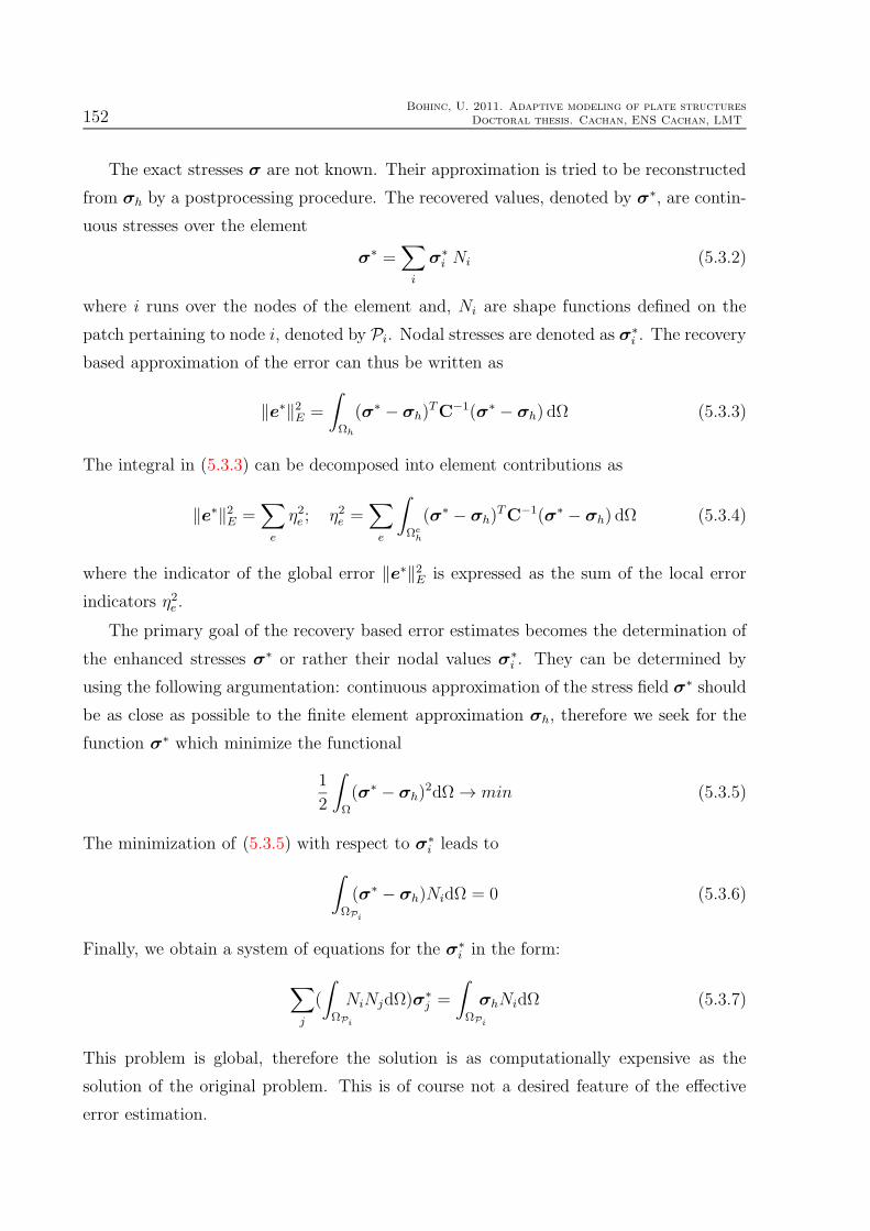
152Bohinc, U. 2011. Adaptive modeling of plate structures
Doctoral thesis. Cachan, ENS Cachan, LMT
The exact stresses σ are not known. Their approximation is tried to be reconstructed
from σh by a postprocessing procedure. The recovered values, denoted by σ∗, are contin-
uous stresses over the element
σ∗ =∑
i
σ∗i Ni (5.3.2)
where i runs over the nodes of the element and, Ni are shape functions defined on the
patch pertaining to node i, denoted by Pi. Nodal stresses are denoted as σ∗i . The recovery
based approximation of the error can thus be written as
‖e∗‖2E =
∫
Ωh
(σ∗ − σh)TC−1(σ∗ − σh) dΩ (5.3.3)
The integral in (5.3.3) can be decomposed into element contributions as
‖e∗‖2E =∑
e
η2e ; η2e =∑
e
∫
Ωeh
(σ∗ − σh)TC−1(σ∗ − σh) dΩ (5.3.4)
where the indicator of the global error ‖e∗‖2E is expressed as the sum of the local error
indicators η2e .
The primary goal of the recovery based error estimates becomes the determination of
the enhanced stresses σ∗ or rather their nodal values σ∗i . They can be determined by
using the following argumentation: continuous approximation of the stress field σ∗ should
be as close as possible to the finite element approximation σh, therefore we seek for the
function σ∗ which minimize the functional
1
2
∫
Ω
(σ∗ − σh)2dΩ → min (5.3.5)
The minimization of (5.3.5) with respect to σ∗i leads to
∫
ΩPi
(σ∗ − σh)NidΩ = 0 (5.3.6)
Finally, we obtain a system of equations for the σ∗i in the form:
∑
j
(
∫
ΩPi
NiNjdΩ)σ∗j =
∫
ΩPi
σhNidΩ (5.3.7)
This problem is global, therefore the solution is as computationally expensive as the
solution of the original problem. This is of course not a desired feature of the effective
error estimation.
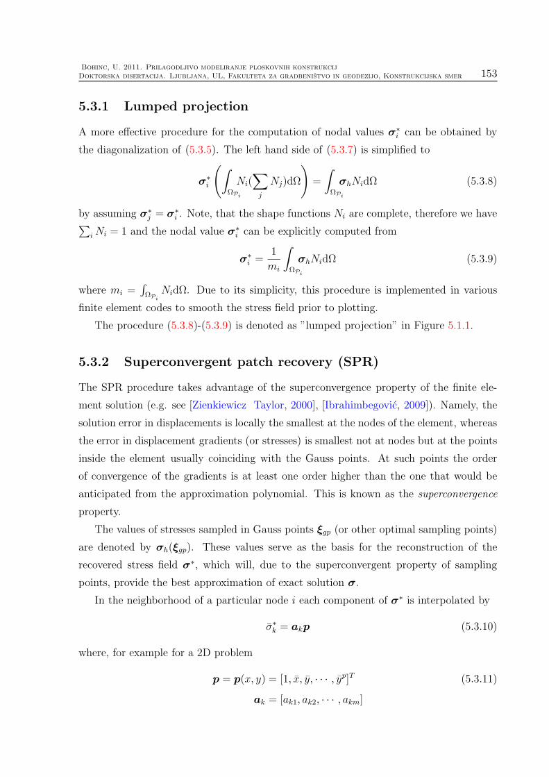
Bohinc, U. 2011. Prilagodljivo modeliranje ploskovnih konstrukcij
Doktorska disertacija. Ljubljana, UL, Fakulteta za gradbenistvo in geodezijo, Konstrukcijska smer 153
5.3.1 Lumped projection
A more effective procedure for the computation of nodal values σ∗i can be obtained by
the diagonalization of (5.3.5). The left hand side of (5.3.7) is simplified to
σ∗i
(∫
ΩPi
Ni(∑
j
Nj)dΩ
)=
∫
ΩPi
σhNidΩ (5.3.8)
by assuming σ∗j = σ∗
i . Note, that the shape functions Ni are complete, therefore we have∑
iNi = 1 and the nodal value σ∗i can be explicitly computed from
σ∗i =
1
mi
∫
ΩPi
σhNidΩ (5.3.9)
where mi =∫ΩPi
NidΩ. Due to its simplicity, this procedure is implemented in various
finite element codes to smooth the stress field prior to plotting.
The procedure (5.3.8)-(5.3.9) is denoted as ”lumped projection” in Figure 5.1.1.
5.3.2 Superconvergent patch recovery (SPR)
The SPR procedure takes advantage of the superconvergence property of the finite ele-
ment solution (e.g. see [Zienkiewicz Taylor, 2000], [Ibrahimbegovic, 2009]). Namely, the
solution error in displacements is locally the smallest at the nodes of the element, whereas
the error in displacement gradients (or stresses) is smallest not at nodes but at the points
inside the element usually coinciding with the Gauss points. At such points the order
of convergence of the gradients is at least one order higher than the one that would be
anticipated from the approximation polynomial. This is known as the superconvergence
property.
The values of stresses sampled in Gauss points ξgp (or other optimal sampling points)
are denoted by σh(ξgp). These values serve as the basis for the reconstruction of the
recovered stress field σ∗, which will, due to the superconvergent property of sampling
points, provide the best approximation of exact solution σ.
In the neighborhood of a particular node i each component of σ∗ is interpolated by
σ∗k = akp (5.3.10)
where, for example for a 2D problem
p = p(x, y) = [1, x, y, · · · , yp]T (5.3.11)
ak = [ak1, ak2, · · · , akm]

154Bohinc, U. 2011. Adaptive modeling of plate structures
Doctoral thesis. Cachan, ENS Cachan, LMT
and x = x − xi, y = y − yi with xi = (xi, yi) denoting the coordinates of node i. The
nodal parameters σ∗i are taken simply as the value of σ∗ at the node i
σ∗i = σ∗(xi) (5.3.12)
The parameters ak are determined using the least square fit of σ∗ to the values σh(xgp)
sampled in the ngp superconvergent points xgp = (xgp, ygp) over the patch of elements
surrounding node i. For each stress component k we have
1
2
ngp∑
gp=1
(σh,k(xgp)− σ∗k(xgp))
2 7−→ min. (5.3.13)
This leads to a small set of linear algebraic equations for the coefficients ak
Mak = b; M = [Mij ]; b = [bi] (5.3.14)
Mij =∑
gp
pi(xgp) pj(xgp); bi =∑
gp
σh,k(xgp)pi(xgp)
The approximation σ∗ is superconvergent in each Gauss integration point in a case
of regular mesh with rectangular elements. For the elements with distorted geometry
the superconvergence is no longer exactly satisfied at the Gauss points. However, the
procedure gives reasonably good approximation even in such cases. An overview of the
SPR procedure is given in Box 1.
Box 1 : The superconvergent patch recovery - SPRAlgoritem 1: SPR metoda
1. Obtain original finite element solution uh of the problem (5.2.4) and obtain σh(xgp)
2. Chose interpolation (5.3.10) of each σ∗k in the neighborhood of node i
3. Evaluate [Mij ] and [bi] from (5.3.14)
4. Solve (5.3.14) for ak
5. Define σ∗i from (5.3.12)
6. Use the interpolation (5.3.2) to get σ∗

Bohinc, U. 2011. Prilagodljivo modeliranje ploskovnih konstrukcij
Doktorska disertacija. Ljubljana, UL, Fakulteta za gradbenistvo in geodezijo, Konstrukcijska smer 155
Figure 5.3.1: SPR recovery of the enhanced stress σ∗I at node I
Slika 5.3.1: Izracun izboljsanih napetosti σ∗I v vozliscih I po metodi SPR
5.4 Residual based error estimates
5.4.1 Explicit
One can find an estimate for the global error in the energy norm (5.2.9) by explicit residual
based error estimates. They are based on the the direct computation of the interior element
residuals and the jumps at the element boundaries. The basic idea of residual based error
estimates comes from the observation that the residual R(uh, v) = a(uh, v) − l(v) is
directly related to the error eh. From (5.2.1) and (5.2.7) if follows that the error satisfies
the equation
a(eh, v) = l(v)− a(uh, v); ∀v ∈ V0 (5.4.1)

156Bohinc, U. 2011. Adaptive modeling of plate structures
Doctoral thesis. Cachan, ENS Cachan, LMT
where v belongs to the test space and it holds true for an arbitrarily chosen test function
v ∈ V0. The integrals in (5.4.1) are split into element contributions:
a(eh, v) =∑
e
le(v)− ae(uh, v); ∀v ∈ V0 (5.4.2)
The forms le and ae are:
ae(uh, v) =
∫
Ωe
[σ(uh)] : [ε(v)] dΩ (5.4.3)
=
∫
Γe
([σ(uh)]n) · v dΓ−∫
Ωe
(∇ · [σ(uh)]) · v dΩ
le(v) =
∫
ΓeN
v · t dΓ +
∫
Ωe
f · v dΩ (5.4.4)
where the Gauss statement was used to perform integration per partes in (5.4.3). The
divergence of stress tensor [σ] is denoted by ∇ · [σ] and the normal to the element side
is denoted by n. The sides with Neumann boundary conditions are denoted by ΓeN
(Γe = ΓeN
⋃ΓeD).
Using the definitions (5.4.3) and (5.4.4), the expression (5.4.2) transforms to
a(eh, v) =∑
e
∫
Ωe
(f +∇ · [σ(uh)])dΩ (5.4.5)
+∑
e
∫
ΓeN
(t− [σ(uh)]n) · v dΩ
+∑
e
∫
ΓeD
([σ(uh)]n) · v dΓ
With the rearrangement of the summation it is possible to split the residual (5.4.5) into
element and side contributions:
a(eh, v) =∑
Ωe
∫
Ωe
RΩe(uh) · v dΩ +∑
Γ
∫
Γ
RΓ(uh) · v dΓ (5.4.6)
RΩe = f +∇ · [σ(uh)]; RΓ =
[[[σ(uh)]n]] ∀Γ ∈ Γe
t− [σ(uh)]n ∀Γ ∈ ΓeN
0 ∀Γ ∈ ΓeD
(5.4.7)
The jump term, denoted by [[·]], is related to the edge Γ, adjacent to elements ei and ej ,
and is defined as
[[σ(uh) · n]]Γ = [σei(uh)] · nei + [σej (uh)] · nej (5.4.8)
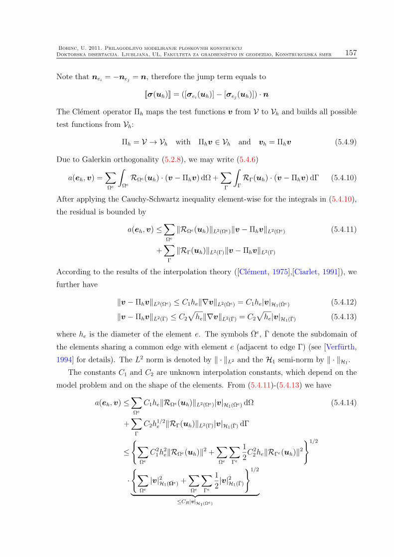
Bohinc, U. 2011. Prilagodljivo modeliranje ploskovnih konstrukcij
Doktorska disertacija. Ljubljana, UL, Fakulteta za gradbenistvo in geodezijo, Konstrukcijska smer 157
Note that nei = −nej = n, therefore the jump term equals to
[[σ(uh)]] = ([σei(uh)]− [σej (uh)]) · n
The Clement operator Πh maps the test functions v from V to Vh and builds all possible
test functions from Vh:
Πh = V → Vh with Πhv ∈ Vh and vh = Πhv (5.4.9)
Due to Galerkin orthogonality (5.2.8), we may write (5.4.6)
a(eh, v) =∑
Ωe
∫
Ωe
RΩe(uh) · (v − Πhv) dΩ +∑
Γ
∫
Γ
RΓ(uh) · (v − Πhv) dΓ (5.4.10)
After applying the Cauchy-Schwartz inequality element-wise for the integrals in (5.4.10),
the residual is bounded by
a(eh, v) ≤∑
Ωe
‖RΩe(uh)‖L2(Ωe)‖v − Πhv‖L2(Ωe) (5.4.11)
+∑
Γ
‖RΓ(uh)‖L2(Γ)‖v − Πhv‖L2(Γ)
According to the results of the interpolation theory ([Clement, 1975],[Ciarlet, 1991]), we
further have
‖v − Πhv‖L2(Ωe) ≤ C1he‖∇v‖L2(Ωe) = C1he|v|H1(Ωe) (5.4.12)
‖v − Πhv‖L2(Γ) ≤ C2
√he‖∇v‖L2(Γ) = C2
√he|v|H1(Γ) (5.4.13)
where he is the diameter of the element e. The symbols Ωe, Γ denote the subdomain of
the elements sharing a common edge with element e (adjacent to edge Γ) (see [Verfurth,
1994] for details). The L2 norm is denoted by ‖ · ‖L2 and the H1 semi-norm by ‖ · ‖H1.
The constants C1 and C2 are unknown interpolation constants, which depend on the
model problem and on the shape of the elements. From (5.4.11)-(5.4.13) we have
a(eh, v) ≤∑
Ωe
C1he‖RΩe(uh)‖L2(Ωe)|v|H1(Ωe) dΩ (5.4.14)
+∑
Γ
C2h1/2e ‖RΓ(uh)‖L2(Γ)|v|H1(Γ) dΓ
≤∑
Ωe
C21h
2e‖RΩe(uh)‖2 +
∑
Ωe
∑
Γe
1
2C2
2he‖RΓe(uh)‖21/2
·∑
Ωe
|v|2H1(Ωe) +∑
Ωe
∑
Γe
1
2|v|2H1(Γ)
1/2
︸ ︷︷ ︸≤CR|v|H1(Ω
e)

158Bohinc, U. 2011. Adaptive modeling of plate structures
Doctoral thesis. Cachan, ENS Cachan, LMT
The H1 semi-norm can be estimated with the energy norm by ‖v‖H1 ≤ CS‖v‖E , whereCS is the stability constant and the energy norm ‖v‖E =
√a(v, v). If the model problem
does not involve any singularities or boundary layers, usually the value CS = 1 is taken.
The constant CR depends on the maximum number of elements in Γe and Ωe. The global
energy norm of the error follows:
‖eh‖2E ≤ CRCS∑
Ωe
C1h2e‖RΩe‖L2(Ωe) +
∑
Ωe
∑
Γe
C2he‖RΓe‖2L2(Γe) (5.4.15)
Finally the explicit residual based error estimate is:
‖eh‖2E ≤∑
e
η2e ; η2e = c1h2e‖RΩe‖L2(Ωe) +
∑
Γe
c2he‖RΓe(uh)‖2L2(Γe) (5.4.16)
where the local error indicator is denoted by ηe.
The constants C1 and C2 are in general unknown. For general linear elastic analysis,
the constants cannot be calculated with a reasonable computational effort. It has to
be pointed that the introduction of the Cauchy-Schwarz inequality severely affects the
accuracy of the error estimate. Therefore, the best possible constants C1 and C2 do not
considerably improve the overall accuracy.
5.4.2 Implicit
The element residual method follows from the work of [Bank Weiser, 1985], [Stein Ohn-
imus, 1997], [Stein Ohnimus, 1999], [Stein et al., 2004]. The interest in implicit schemes
stems from the fact that in explicit schemes the whole information for the total error is
obtained only from the given solution uh. It is possible to obtain more accurate informa-
tion on the error by solving additional auxiliary problems. Implicit error estimates thus
involve the construction of the auxiliary boundary value problems, whose solution yields
an approximation to the actual error.
The boundary problems to be solved are local, which means that they are posed
either on a small patch of elements (subdomain residual method) or even on a single
element (element residual method). In general, a drawback of the subdomain residual
method can be that solving the local problems is rather expensive, since each element is
considered several times. Moreover, the element residual method needs to approximate
the prescribed Neumann boundary conditions on each single element ([Gratsch Bathe,
2005]). In the following, a variant of the element residual method will be presented; so-
called the equilibrated residual method (EqR) (closely related to PEM method introduced
in [Stein Ohnimus, 1997]).

Bohinc, U. 2011. Prilagodljivo modeliranje ploskovnih konstrukcij
Doktorska disertacija. Ljubljana, UL, Fakulteta za gradbenistvo in geodezijo, Konstrukcijska smer 159
The equilibrated residual method (EqR)
From (5.2.1) and (5.2.7) it follows that the error satisfies the equation
a(eh, v) = l(v)− a(uh, v); ∀v ∈ V0 (5.4.17)
This problem can be solved approximately for eh by replacing v with a suitable candidate
and thus furnish an approximation e to the actual error eh. According to (5.2.8), reusing
the finite element subspace Vh to produce such an approximation will result in trivial
solution e = 0. It thus follows, that in order to get non trivial estimate of the error, the
test space should be enhanced with respect to the finite element space.
Solving of global problem (5.4.17) to obtain error estimate is as computationally de-
manding as solving the original problem. Clearly, this is not an optimal choice. For
any practically acceptable procedure, the computation of error estimate should be more
efficient than computation of the global problem. One way to increase the efficiency, is
to replace the global problem with a sequence of uncoupled boundary value problems,
with each one posed over a single element. Doing so, so-called element residual method
is obtained.
Ωe
Γe Γe
e′
I
J
ΓIJ
Figure 5.4.1: Notation
Slika 5.4.1: Oznake
The error equation (5.4.17) can be decomposed into element contributions:
a(eh, v) =∑
e
le(v)− ae(uh, v)+∑
e
∫
Γe
teΓ · v dΓ; ∀v ∈ V0 (5.4.18)
where we indicated that such decomposition is introducing additional boundary tractions
teΓ which act on the edges Γe of all the elements (see Figure 5.4.1). Let two neighboring
elements e and e′ share the edge Γ (Figure 5.4.1). The comparison between (5.4.17) and
(5.4.18) implies ∑
e
∫
Γe
teΓ · v ds = 0. (5.4.19)

160Bohinc, U. 2011. Adaptive modeling of plate structures
Doctoral thesis. Cachan, ENS Cachan, LMT
The equation (5.4.19) requires that the work of boundary tractions from both elements,
adjacent to the edge Γ, cancels out. Considering that the same displacement interpolation
along the edge Γ is shared by adjacent elements, denoted by e and e′, we can further
conclude:
teΓ + te′
Γ = 0. (5.4.20)
With these results, the expression in (5.4.18) can then be replaced by local, element-
wise ones. To that end, let ϑe,h denote the solution of the weak form of the local boundary
value problem for the error computation over the element e:
ae(ϑe,h, v) = le(v)− ae(uh, v) +
∫
Γe
teΓ · v ds; ∀v ∈ V0 (5.4.21)
Note, that the local element problems (5.4.21) for unknown ϑe,h are of Neumann type,
since only tractions teΓ are prescribed on element edges.
Moreover, the boundary tractions teΓ are unknown and are yet to be constructed from
the finite element solution uh, and in agreement with (5.4.20). In this manner, the global
error computation (5.4.1) has been split into element contributions
a(eh, v) =∑
e
ae(ϑe,h, v) (5.4.22)
With the use of the Cauchy-Schwartz inequality, the relation between global error eh and
local solutions ϑe,h, the upper bound of a global error can be estimated
‖eh‖2E ≤∑
e
‖ϑe,h‖2E =∑
e
η2e (5.4.23)
where the local error indicator ηe is defined as
η2e = ‖ϑe,h‖2E (5.4.24)
In the case when element boundary tractions teΓ coincide with the boundary tractions
obtained from the exact solution for the right choice of v ∈ V0, the estimated error is
exact, since the exact solution to (5.4.18) can be recovered. It is thus obvious that the
quality of approximation of element boundary tractions is critical for the effective error
estimate. In the following, an efficient method for building the approximation of true
boundary tractions will be presented.
We first see that the Galerkin orthogonality property (5.2.8) of the finite element
solution uh through the use of (5.4.22) implies ae(ϑe,h, vh) = 0. Then, by using (5.4.21),
an additional constraint for the unknown boundary tractions teΓ can be constructed:∫
Γe
teΓ · vh ds = ae(uh, vh)− le(vh) (5.4.25)

Bohinc, U. 2011. Prilagodljivo modeliranje ploskovnih konstrukcij
Doktorska disertacija. Ljubljana, UL, Fakulteta za gradbenistvo in geodezijo, Konstrukcijska smer 161
The meaning of the equation (5.4.21) becomes more evident if ϑe,h is defined as the
difference between element approximation to the exact solution ue,h, and the FE solution
ue,h
ϑe,h = ue,h − ue,h
Due to linearity of bilinear form a, the local problem (5.4.21) for ue then becomes
ae(ue,h, v) = le(v) +
∫
Γe
teΓ · v ds; ∀v0 ∈ V (5.4.26)
The result ae(ϑe,h, vh) = 0 implies ae(ue,h, vh) = ae(ue,h, vh). It is thus clear that
ue,h = ue,h, when the subspace used to obtain a local solution of (5.4.26) is identical
to the original subspace Vh, which was used to obtain the global finite element solution.
Therefore, to be able to get an error estimate from (5.4.26), an enhanced test space should
be used with vh+ ∈ V.The enhanced space deformation modes should also include rigid body modes vΛ, for
which it holds ae(uh, vΛ) = 0. In this case, the result in (5.4.25) will reduce to∫
Γe
teΓ · vΛ ds+ le(vΛ) = 0 (5.4.27)
By closer inspection of the expression (5.4.27), the equilibrium of the boundary tractions
with the external loading can be deduced in the sense of virtual work principle.
An estimate of the discretization error can then be obtained through the solution
of local problems (5.4.26) of Neumann type where V is replaced by its best possible
approximation Vh+ that must be sufficiently enhanced with respect to Vh
ae(ue,h+, vh+) = le(vh+) +
∫
Γe
teΓ · vh+ ds; vh+ ∈ Vh+ (5.4.28)
The loading of element problems consists of the sum of the external loading and the
boundary tractions teΓ. They are referred to as equilibrated boundary tractions, due to the
property (5.4.27) which implies that they are in equilibrium with the external loading.
In a sense, the equilibrated boundary tractions are introduced to represent the action of
surrounding elements on the selected element. Introduced boundary tractions are contin-
uous across element edges. In summary, the main steps involved in the error estimation
procedure are given in Box 2.
Computation of equilibrated boundary tractions for EqR
The performance of element residual method depends crucially on the estimation of equi-
librated boundary tractions (see Box 2). In the following, a general procedure for the
computation will be presented, which follows the work of [Ladeveze Leguillon, 1983].

162Bohinc, U. 2011. Adaptive modeling of plate structures
Doctoral thesis. Cachan, ENS Cachan, LMT
Box 2 : The equilibrated residual method - EqRAlgoritem 2: EqR metoda
1. Obtain original finite element solution uh of the problem (5.2.4)
2. Compute equilibrated boundary tractions teΓ for each edge Γ ⊂ Γe
of each element e (see Box 3)
3. Approximately solve (5.4.28) for ue,h+ by using test space Vh+ as enhancedapproximation to Vh
4. Compute local error estimates η2e from (5.4.24) and ϑe,h = ue,h+ − ue,h
Recall that j-th component of the test function vh is a linear combination of shape
functions Nj,k and nodal degrees of freedom vk. The interpolation of j-th component of
vh along an edge Γ is thus
(vh|Γ)j =∑
k
Nj,kvk =∑
K
NKj · vK (5.4.29)
The alternative notation (NKj ; vK) refers to a set of the shape functions and interpolation
parameters which pertain in any manner to node K. Specifically, we have vK = [vi,K ]T
and NKj = [NK
j,i]T with i = 1 . . . nndofK , where nndofK is number of degrees of freedom at
node K.
The virtual work of boundary tractions on edge Γ, spanning between nodes I and J ,
can then be reduced to1 :
∫
Γ
teΓ · vh ds = reI,Γ · vI + re
J,Γ · vJ , (5.4.30)
where reI,Γ denotes the “projection” (in a virtual work sense) of boundary traction teΓ to
node I. The components of reI,Γ are directly related to the components of vI . Thus, the
number of components in reI,Γ matches the number of nodal degrees of freedom at node
I.
Let us assume that the boundary tractions teΓ variations are described with some chosen
interpolation. Regarding edge Γ, boundary tractions teΓ, can thus always be recovered from
the projections reI,Γ, r
eJ,Γ:
reI,Γ, r
eJ,Γ ⇒ teΓ (5.4.31)
1We reduce attention to the edge with two vertex nodes, although the edge with more nodes could be
treated in the same manner

Bohinc, U. 2011. Prilagodljivo modeliranje ploskovnih konstrukcij
Doktorska disertacija. Ljubljana, UL, Fakulteta za gradbenistvo in geodezijo, Konstrukcijska smer 163
I JΓ=ΓIJ
teΓreI,Γ re
J,Γ
Figure 5.4.2: Relation between the tractions teΓ and their projections reI,ΓSlika 5.4.2: Relacija med robno obtezbo teΓ in projekcijami rI,Γ
We therefore decide to replace in what follows the unknown tractions teΓ with their pro-
jections reI,Γ. This will enable the patch-wise computation of boundary tractions teΓ.
By using ReI to denote the element nodal residuals2, the right hand side of (5.4.25)
can be rewritten as
ae(uh, vh)− le(vh) = ReI · vI (5.4.32)
Moreover, the continuity condition for boundary tractions (5.4.20) can be rewritten as,
see Figure 5.4.3:
reI,Γ + re′
I,Γ = 0 (5.4.33)
From (5.4.25), (5.4.30) and (5.4.32) we have (with a slight change in notation3), see Figure
5.4.4
reI,Γ1
+ reI,Γ2
= ReI (5.4.34)
where Γ1 and Γ2 are edges of the same element e meeting at node I. Gathering (5.4.33)
and (5.4.34), we obtain a linear system of algebraic equations with the projections reI,Γ as
unknowns. These systems are formed patchwise for the projections reI,Γ of the node I.
To illustrate the patchwise formation of a local system of this kind we inspect an
example with a patch of four 2D elements surrounding node I of the FE mesh (see Figure
5.4.5). Equations (5.4.34) and (5.4.33) for this case read (with a slight abuse of notation):
Re1I = re1
I,Γ4+ re1
I,Γ1re1I,Γ1
+ re2I,Γ1
= 0 (5.4.35)
Re2I = re2
I,Γ1+ re2
I,Γ2re2I,Γ2
+ re3I,Γ2
= 0
Re3I = re3
I,Γ2+ re3
I,Γ3re3I,Γ3
+ re4I,Γ3
= 0
Re4I = re4
I,Γ3+ re4
I,Γ4re4I,Γ4
+ re1I,Γ4
= 0
2Element nodal residuals can also be interpreted as the element nodal reactions i.e. the forces acting
on the nodes of the element.3The edge Γ has sometimes subscript related to the index of the edge; e.g. Γ1, Γ2, · · ·

164Bohinc, U. 2011. Adaptive modeling of plate structures
Doctoral thesis. Cachan, ENS Cachan, LMT
Γ1
Γ2
I
e
reI,Γ1
reI,Γ2
ReI
Figure 5.4.3: Element nodal residual ReI and boundary tractions projections reI,Γ1,2
at node I
of element e
Slika 5.4.3: Vozliscne reakcije ReI elementa in projekcije robnih obtezb reI,Γ1,2
v vozliscu I
elementa e
Γ
I
ereI,Γ
I
e′
re′
I,Γ
Figure 5.4.4: Continuity of boundary tractions projections reI,Γ
Slika 5.4.4: Zveznost projekcij robnih obtezb reI,Γ
Note, that the equations (5.4.35) also imply the node equilibrium∑
eiRei
I = 0. Combining
the last set of equations, we obtain the following system of equations with the only
remaining unknowns rekI,Γk
Re1I
Re2I
Re3I
Re4I
=
+1 0 0 −1−1 +1 0 00 −1 +1 00 0 −1 +1
re1I,Γ1
re2I,Γ2
re3I,Γ3
re4I,Γ4
(5.4.36)
Unfortunately, the local system in (5.4.36) is singular and its solution is not unique.
To obtain the unique solution, a regularization has to be used. In the following, the
regularization introduced in ([Stein Ohnimus, 1999], [Ainsworth Oden, 2000]) will be
used.

Bohinc, U. 2011. Prilagodljivo modeliranje ploskovnih konstrukcij
Doktorska disertacija. Ljubljana, UL, Fakulteta za gradbenistvo in geodezijo, Konstrukcijska smer 165
e1
e2e3
e4
I
Re1I
re1I,Γ1
re1I,Γ4
Re2I
re2I,Γ1
re2I,Γ2
Re3I
re3I,Γ2
re3I,Γ3
Re4I
re4I,Γ4
re4I,Γ3
Γ4
Γ1
Γ2
Γ3
Figure 5.4.5: Patch PI of four elements around node I
Slika 5.4.5: Krpa PI stirih elementov okoli vozlisca I
Regularization of (5.4.33), (5.4.34)
First, an alternative estimate for the boundary tractions which will be denoted as teΓ has
to be constructed. Next, we use (5.4.30) to compute the projections reI,Γ:
∫
Γ
teΓ · vh ds = reI,Γ · vI + re
J,Γ · vJ , (5.4.37)
The basic idea of the regularization is to seek for the projections reI,Γ which are as close
as possible, in a least squares sense, to the projections reI,Γ. Hence, beside imposing
the constraints (5.4.33) and (5.4.34), we will seek for the projections reI,Γ that minimize
the objective function over a patch PI around node I (a slight change in notation is

166Bohinc, U. 2011. Adaptive modeling of plate structures
Doctoral thesis. Cachan, ENS Cachan, LMT
introduced4)1
2
∑
e∈PI
∑
ΓIK
(reI,ΓIK
− reI,ΓIK
)2 7−→ min. (5.4.38)
The alternative boundary tractions teΓ are usually computed from the stresses σh(uh).
Since the finite element stresses σh are discontinuous over the edges of the elements their
continuity is first enforced. Simple averaging can be performed
σ|Γ = (σeh|Γ + σe′
h |Γ)/2 (5.4.39)
The alternative boundary tractions are then
teΓ = [σ|Γ]neΓ (5.4.40)
The procedure for the determination of the equilibrated boundary tractions is summarized
in Box 3:
Box 3 : Computation of equilibrated boundary tractionsAlgoritem 3: Uravnotezenje robnih obtezb
1. Compute element nodal residuals ReI from uh using (5.4.32)
2. Construct teΓ from (5.4.40) and (5.4.39)
3. Compute alternative projections reI,Γ from (5.4.37)
4. Form patchwise systems of equations (5.4.35) and solve them for reI,Γ by (5.4.38)
5. Choose the interpolation ψIk, ψ
Jk for boundary tractions teΓ and solve for nodal values
of boundary tractions peΓ,I from (5.4.43)
6. Compute boundary tractions by (5.4.40)
Let us now elaborate on Step 5 in Box 2 and introduce parametrization of k-th com-
ponent of the boundary traction teΓ (let Γ be element edge between element nodes I and
J) as
(teΓ)k = ψIkpk,I + ψJ
k pk,J (5.4.41)
where ψIk are interpolation functions (yet to be chosen) and pk,I are the nodal values of
(teΓ)k. The variation of virtual displacements along the edge Γ can be written as
(vh,Γ)k =
nndofI∑
i=1
N Ik,ivi,I +
nndofJ∑
i=1
NJk,ivi,J (5.4.42)
4The edge Γ (see Figure 5.4.2) has sometimes subscript related to the indices of vertex nodes of the
edge: e.g. ΓIJ , ΓIK , · · ·

Bohinc, U. 2011. Prilagodljivo modeliranje ploskovnih konstrukcij
Doktorska disertacija. Ljubljana, UL, Fakulteta za gradbenistvo in geodezijo, Konstrukcijska smer 167
where vj,I is related to the j-th degree of freedom at node I, and N Ik,i are the corresponding
shape functions. In other words, the shape function N Ik,i interpolates the k-th component
of virtual displacements vh,Γ and is weighted by nodal degree of freedom vi,I in the linear
interpolation (5.4.42). We can now insert the above parameterizations into (5.4.30) and
express residuals at nodes I and J with respect to the boundary traction on edge Γ (that
spans between I and J). The result can be written in a compact form as:
[reI,Γ
reJ,Γ
]=
[MII
Γ MIJΓ
MJIΓ MJJ
Γ
] [pΓ,I
pΓ,J
]; (5.4.43)
MIJΓ = [MI,J
Γ ]; MI,JΓ = [M I,J
Γ,nm]
where pΓ,I = [pk,I ]T , k = 1, . . . ndim, and ndim is a dimension of teΓ. The block matrices
MI,JΓ have nndofI rows and ndim columns with the elements
M I,JΓ,nm =
∫
Γ
N Im,nψ
Jmds (5.4.44)
The index m is denotes the virtual displacement component which is conjugated (in the
sense of the virtual work principle) to the traction component m.
By solving (5.4.43) for every element edge Γ, we obtain parameters pΓ,I and pΓ,J ,
which completely define element boundary traction teΓIJthrough (5.4.41). The choice of
the shape functions ψIk, which describe the variation of the boundary tractions along the
edge, is somewhat arbitrary. It is suggested in the literature (e.g. [Ainsworth Oden,
2000], [Oden Cho, 1997]) that shape functions ψJk and ψI
k should be orthogonal to the
shape functions describing the variation of the test function vh. In this case the terms
MIJΓ and MJI
Γ vanish and the matrix M becomes block diagonal. The relation (5.4.43)
simplifies to
reI,Γ = MII
Γ pIΓ (5.4.45)
which significantly reduces the computation cost. Note, however, that the specific choice
of parametrization (5.4.45) does not affect the local patch-wise computation of boundary
tractions.

168Bohinc, U. 2011. Adaptive modeling of plate structures
Doctoral thesis. Cachan, ENS Cachan, LMT
1
2
3Re
3
Re1
Re1
Γe12
Γe23
Γe31
Ωe
1
2
3Re
3
Re1
Re1
Γe12
Γe23
Γe31
Ωe
re1,Γ31
re1,Γ12
re2,Γ12
re2,Γ23
re3,Γ23
re3,Γ31
Figure 5.4.6: Representation of element nodal residuals ReI by the projections reI,Γ
Slika 5.4.6: Vozliscne reakcije elementa ReI in projekcije reI,Γ robne obtezbe teΓ
1
2
3Re
3
Re1
Re1
Γe12
Γe23
Γe31
Ωe
re1,Γ31
re1,Γ12
re2,Γ12
re2,Γ23
re3,Γ23
re3,Γ31
1
2
3
Γe12
Γe23
Γe31
teΓ12
teΓ23
teΓ31
Ωe
Figure 5.4.7: Boundary tractions teΓ replace the action of element projections reI,Γ
Slika 5.4.7: Robna obtezba teΓ je po principu virtualnega dela ekvivalentna delovanju projekcij
reI,Γ (in s tem tudi ReI)

Bohinc, U. 2011. Prilagodljivo modeliranje ploskovnih konstrukcij
Doktorska disertacija. Ljubljana, UL, Fakulteta za gradbenistvo in geodezijo, Konstrukcijska smer 169
L
x g
ρ, E,A = A(x)
Governing equations:d(σA)dx
= ρgA; σ = Eε; ε = dudx
Boundary conditions: u(x = 0) = 0
Weak form: a(u, v) = l(v); ∀v ∈ V0
a(u, v) =∫ L
0EAdu
dxdvdxdx;
l(v) =∫ L
0ρgAvdx
Discretization:uh =
∑e u
eh; u
eh =
∑I N
eI u
eI ;
vh =∑
e veh; v
eh =
∑I N
eI v
eI
Figure 5.5.1: One dimensional problem: hanging bar with variable cross sectionSlika 5.5.1: Enodimenzionalni problem: viseca palica s spremenljivim presekom
5.5 Illustration of SPR and EqRmethods on 1D prob-
lem
In the following, the basic principles of EqR and SPR error estimates will be illustrated on
a simple one-dimensional problem. The illustration of the error estimation methods on a
simple problem reveals the fundamental differences in the concepts. The one-dimensional
problem also clearly identifies the key steps of the computation procedures.
The subject of a model problem is a hanging bar with a variable cross section A. The
bar of length L is made of linear elastic material with the modulus of elasticity E and
density ρ (see Figure 5.5.1).
The displacement of the bar along the x axis is denoted by u. The deformation is
ε = dudx. Hooke’s law gives the stress σ = Eε. The line force Aρg (g is earth acceleration)
is equilibrated by the axial force σA:
d(σA)
dx= ρgA
The summary of governing equations is given in Figure 5.5.1.
The displacement of the bar u is discretized by the function uh =∑
e ueh. We introduce
linear and quadratic finite elements. The linear element has two degrees of freedom ue1
and ue2 at vertex nodes 1 and 2. The nodal coordinates are denoted by xe1 and xe2. The
displacement of linear element is approximated by ueh = ueh,L = N e1 u
e1 +N e
2 ue2, where N
e1

170Bohinc, U. 2011. Adaptive modeling of plate structures
Doctoral thesis. Cachan, ENS Cachan, LMT
and N e2 are defined as:
N e1 (x) =
xe2 − x
Le; N e
2 (x) =x− xe1Le
; N e3 (x) = 4N e
1 (x)Ne2 (x) (5.5.1)
where Le denotes the length of the element. The quadratic element has an additional
degree of freedom ue3 at the middle point of the element xe3 = (xe1 + xe2)/2. The approx-
imation of displacement of a quadratic element is a hierarchic extension of that of the
linear element ueh = ueh,Q = ueh,L +N e3 u
e3.
The finite element solution uh satisfies
a(uh, vh) = l(vh); ∀vh ∈ Vh (5.5.2)
The test functions vh are interpolated as vh =∑
e veh, where v
eh =
∑I N
eI v
eI the sum runs
over all the degrees of freedom. The shape function Nk is related to the degree of freedom
k and is defined as the sum of element shape functions Nk =∑
eNeI pertaining to the
chosen degree of freedom. The set of equations defining the solution , which follows from
(5.5.2), is:
a(uh, Nk) =∑
e
ae(ueh, Nk) = l(Nk); ∀Nk (5.5.3)
The element stiffness matrix and the load vector are introduced to enable the matrix
notation of (5.5.3). They are defined as:
KeIJ = ae(N
eJ , N
eI ) =
∫ xe2
xe1
EAdN e
J
dx
dN eI
dxdx; (5.5.4)
F eI = l(N e
I ) =
∫ xe2
xe1
ρgAN eI dx (5.5.5)
In the example below we are solving for the displacement of the tapered hanging bar of
the cross section A = A0(1+ p−12p(1−x/L)2x/L), where p is the taper parameter. The
linear and quadratic solutions for the case p = 1 are shown in Figure 5.5.2 and Figure
5.5.3 (u0 = ρgL2/(2E) and σ0 = ρgL are values of maximum displacement and stress
for the case p = 0 - rod with constant cross section). The significant variation of cross
section is reflected in rich stress variation. Relatively small number of elements (5), which
are used to obtain the finite element solution, enable to visually asses the quality of the
solution in terms of displacement as well as in terms of the stress. As expected, significant
stress jumps occur in the case of linear elements, whereas quadratic elements capture the
variation of stress much better. The stress jumps between the elements are in this case
smaller, although they do not vanish completely.

Bohinc, U. 2011. Prilagodljivo modeliranje ploskovnih konstrukcij
Doktorska disertacija. Ljubljana, UL, Fakulteta za gradbenistvo in geodezijo, Konstrukcijska smer 171
u
uh,L
σ/σ0
σh,L/σ0
0.2 0.4 0.6 0.8 1.0
0.2
0.4
0.6
0.8
1.0
1.2
0.2 0.4 0.6 0.8 1.0
0.5
1.0
1.5
2.0
2.5
3.0
3.5
σ/σ0u/u0
x/Lx/L
Figure 5.5.2: Solution of the model problem with linear elementsSlika 5.5.2: Resitev modelnega problema z linearnimi elementi
u
uh,Q
σ/σ0
σh,L/σ0
0.2 0.4 0.6 0.8 1.0
0.2
0.4
0.6
0.8
1.0
1.2
0.2 0.4 0.6 0.8 1.0
0.5
1.0
1.5
2.0
2.5
3.0
3.5
σ/σ0u/u0
x/Lx/L
Figure 5.5.3: Solution of the model problem with quadratic elementsSlika 5.5.3: Resitev modelnega problema s kvadraticnimi elementi
First, we compute the error of linear elements by the SPR procedure. Enhanced
stress σ∗ is computed from the original finite element solution. Since the problem is one-
dimensional, the nodal values of enhanced stress σ∗ are effectively computed as the average
of the integration point values of stress of two neighboring elements. The integration
point (with superconvergent properties) is taken at the midside of the element. In Figure
5.5.4 the enhanced stress is depicted as solid blue line and the nodal values of enhanced
stress are shown as red points. Note, that the SPR method, although better than the
original finite element stress estimate, is unable to fully capture the variation of the exact
(analytic) stress (shown as gray dashed line). The key feature of the method - averaging
of discontinuous stress field - can clearly be recognized.
Next, we compute the error of linear elements by the EqR procedure. The EqR com-
putation of the enhanced stress σ∗ is based on local element computations with enhanced

172Bohinc, U. 2011. Adaptive modeling of plate structures
Doctoral thesis. Cachan, ENS Cachan, LMT
σ/σ0
σh,L/σ0
σ∗SPR/σ0æ
æ
æ
æ
æ
æ
0.2 0.4 0.6 0.8 1.0
0.5
1.0
1.5
2.0
2.5
3.0
3.5
σ/σ0
x/L
(SPR)
σ/σ0
σh,L/σ0
σ∗EqR/σ0
æ
æ
æ
æ
æ
æ
0.2 0.4 0.6 0.8 1.0
0.5
1.0
1.5
2.0
2.5
3.0
3.5
σ/σ0
x/L
(EqR)
Figure 5.5.4: Computation of enhanced stress σ∗; comparison of SPR and EqR method
Slika 5.5.4: Izracun izboljsanih napetosti σ∗; primerjava med SPR in EqR metodo
model. The boundary conditions for the element problems are of Neumman type and
are computed from the current finite element solution. The nodal element residuals are
computed from Re = [Re1, R
e2]
T = KeLu
e−F eL, where L denotes the linear element. In the
simple one-dimensional model no additional equilibration is needed and the reactions Re1
and Re2 are already the nodal forces used in the local element computation. Since we are
using the quadratic element as the enhanced model, the load vector is Re = [Re1, R
e2, 0]
T .
Enhanced element stresses σ∗ are finally computed from the solutions ue of the local
element problems:
KeQu
e = Re + F eQ
Figure 5.5.4-(EqR) depicts the enhanced stress σ∗ computed from ue. The red points
show the values |Re|/A, which can be interpreted as the nodal stress values σ∗I . Note that
they coincide with true nodal stress values σI . Also the enhanced stresses σ∗ show very
good overall agreement of the true ones computed from analytical solution.
5.6 Chapter summary and conclusions
The chapter is concerned with the computation of discretization error in general. An
overview of existing a-posteriori methods is given. Among them, two are covered in detail:
the superconvergent patch recovery method (SPR) and the equilibrated residual method
(EqR). Both methods are treated to the level ready for the implementation. The treatment

Bohinc, U. 2011. Prilagodljivo modeliranje ploskovnih konstrukcij
Doktorska disertacija. Ljubljana, UL, Fakulteta za gradbenistvo in geodezijo, Konstrukcijska smer 173
of SPR and EqR method is accompanied with a small illustrative numerical example.
The detailed, independent and systematic treatment of the EqR method revealed some
important results relevant for the application of the method to the modeling of plate
structures. The main step in the EqR method is the computation of the admissible
boundary tractions for the local problem. Perhaps the key finding of this chapter is, that
the interpolation of the boundary tractions does not enter the equilibration procedure
directly. The equilibration procedure is computed independently on the level of boundary
traction projections. The specific form of the interpolation of boundary tractions enters
the computation only through the regularization.

174Bohinc, U. 2011. Adaptive modeling of plate structures
Doctoral thesis. Cachan, ENS Cachan, LMT

Bohinc, U. 2011. Prilagodljivo modeliranje ploskovnih konstrukcij
Doktorska disertacija. Ljubljana, UL, Fakulteta za gradbenistvo in geodezijo, Konstrukcijska smer 175
Chapter 6
Discretization error for DK and RMelements
6.1 Introduction
There exist a very large number of applications from aerospace, civil and mechanical engi-
neering, which call for the plate finite element (FE) models. Among plate finite elements,
perhaps the most frequently used, are the discrete-Kirchhoff (DK) finite elements for thin
plates (e.g. see [Batoz et al., 1980], [Batoz, 1982] or [Bernadou, 1996]). These elements
deliver near optimal performance for thin plate element with the smallest possible num-
ber of nodes. Thus they are used in practically any commercial code, either as 3-node
triangle (DKT) or as 4-node quadrilateral (DKQ). Hence, the main question addressed
in this chapter, pertaining to discretization error and choice of the FE mesh size when a
plate is discretized by DK elements, is of great practical importance.
The DK plate element, delivering optimal performance, is the result of the long line
of developments on Kirchhoff-Love plate FE models (such as [Clough Tocher, 1965] or
[Felippa Clough, 1965]) that also benefited from more recent works on Reissner/Mindlin
thick plate FE models (e.q. see [Zienkiewicz Taylor, 2000] and references herein). How-
ever, as opposed to shear locking phenomena of Reissner/Mindlin FE plate models (e.q.
see [Zienkiewicz Taylor, 2000] or [Hughes, 2000], Taylor et al [Zienkiewicz Taylor, 2000]),
the DK plate model completely removes the shear deformation and thus eliminates the
locking. This results with non-conventional FE interpolations with C1 continuity (e.q. see
[Ibrahimbegovic, 1993]). Therefore, most of the previous results on error estimates, com-
ing from solid mechanics FE models with C0-interpolations (e.g. see [Ainsworth Oden,
2000], [Ladeveze Pelle, 2006] or [Stein Ramm, 2003]), do not directly apply to this case.
Moreover, the non-conventional FE interpolations of DK plate elements are the result of

176Bohinc, U. 2011. Adaptive modeling of plate structures
Doctoral thesis. Cachan, ENS Cachan, LMT
enforcing the Kirchhoff constraint selectively, and they are not based on the minimum
energy principles. For all these reasons, it is not easy to provide the error estimates for
DK plate elements with rigorous upper and lower bounds, but rather the most useful error
indicators.
In this chapter we present the error estimates and indicators for DK plate elements
based upon two main families, the superconvergent patch recovery (e.g. see [Zienkiewicz
Zhu, 1992], [Babuska Pitkaranta, 1990]) and the equilibrated residual method (e.g. see
[Becher Rannacher, 2001], [Johnson Hansbo, 1992] or [Ladeveze Leguillon, 1983]). In
what follows, we will not, strictly distinguish between error estimates and error indicators.
It turns out that the superconvergent patch recovery procedure is easy to apply to
discrete-Kirchhoff plate elements, by constructing the enhanced approximation through
superconvergence property of Gauss point values (e.g. see [Zienkiewicz Taylor, 2000],
[Flajs et al., 2010]). On the contrary, the equilibrated residual method needs somewhat
more ingenious procedure. Namely, it was found out, that the best estimate of the exact
solution is constructed by using the plate elements suggested by Argyris and co-workers
(see [Argyris et al., 1968]) that have been used by mathematicians (see [Bernadou, 1996])
but never reached the wide acceptance by engineers.
At the end of the chapter we show that the error estimates and indicators for Reiss-
ner/Mindlin (RM) plate elements can be obtained in a very similar way as it is presented
here for DK elements.
6.2 Discretization error for DK elements
The local error indicator for the DK elements is computed from
η2e,DK =∑
e
∫
Ωeh
(m∗ −mh)TC−1
B (m∗ −mh) dΩ (6.2.1)
where m∗ are the enhanced moments. They are computed using either SPR method or
the EqR method. In the case of EqR method, the enhanced moments are computed from
the solution of the local problems ue,h: m∗ = m∗(ue,h).
1
6.2.1 Discrete approximation for error estimates
The computation of the equilibrated boundary tractions, which represent the input data
for the element problems in EqR method, is defined in Box 3. Steps 1 and 3 do not,
1The definition of the local error indicator (6.2.1) follows from (5.4.24) and is equivalent to (5.3.4).

Bohinc, U. 2011. Prilagodljivo modeliranje ploskovnih konstrukcij
Doktorska disertacija. Ljubljana, UL, Fakulteta za gradbenistvo in geodezijo, Konstrukcijska smer 177
besides the topology, change with respect to the element used. The steps 2 and 4 depend
on the interpolation. The main issue becomes the relation between boundary tractions teΓ
and their projections reI,Γ.
Let us recall the interpolation of displacement and rotations over the edges of the
element. The variation of displacement along the element boundary ΓIJ , spanned between
the element nodes I and J , is defined (according to (2.3.59)) by:
wh,ΓIJ= wI ϕ1 + wJ ϕ2 +
LIJ
4nIJ · (θI − θJ) ϕ3 +
LIJ
3∆θIJ ϕ4 (6.2.2)
where ∆θIJ = 32 LIJ
(wJ − wI) − 34nIJ · (θI + θJ), LIJ is the length of the edge ΓIJ
and nIJ = [nx,IJ , ny,IJ ]T is the unit exterior normal and φ1, · · · , φ4 are shape functions.
Similarly, variation of rotation vector along the same edge can be written as
θh,ΓIJ= θI ϕ1 + θJ ϕ2 + nIJ∆θIJ ϕ3 (6.2.3)
The shape functions ϕi in (6.2.2) and (6.2.3) are defined as, see (2.3.55)
ϕ1 = (1− ξ)/2 ϕ2 = (1 + ξ)/2 (6.2.4)
ϕ3 = (1− ξ2)/2 ϕ4 = ξ(1− ξ2)/2,
where ξ ∈ [−1, 1].
We compute the boundary traction projections reI,ΓIJ
, which pertain to the boundary
tractions teΓIJ= [qef , ms, mn] through (5.4.30).
In order to evaluate the traction projections, the following integral has to be evaluated:∫
ΓIJ
(qef,ΓIJ
wh,ΓIJ+ms,ΓIJ
(s · θh,ΓIJ))ds+ [mnwh,ΓIJ
]JI = reI,ΓIJ
· uI + reJ,ΓIJ
· uJ (6.2.5)
Comparison of the corresponding terms on both sides of the equation (6.2.5) will provide
the components of the projections reI,Γ = [rwI,Γ, r
θxI,Γ, r
θyI,Γ]
T , where the notation Γ = ΓIJ
is employed. These components are energy conjugated to the plate element degrees of
freedom and the chosen discretization.
The boundary traction teΓ consists of three components: shear qΓ and moments ms,Γ,
mn,Γ. For the given interpolation for teΓ, the components can be reconstructed from the
projections reI,Γ from (7.2.25). We chose to interpolate each of the components of teΓ with
the same interpolation: a linear combination of the shape functions ψI and ψJ :
qΓ = qIΓψI + qJΓψJ (6.2.6)
ms,Γ = mIs,ΓψI +mJ
s,ΓψJ
mn,Γ = mIn,ΓψI +mJ
n,ΓψJ

178Bohinc, U. 2011. Adaptive modeling of plate structures
Doctoral thesis. Cachan, ENS Cachan, LMT
Note, that qef,Γ in (6.2.5) is defined as qΓ − ∂mn,Γ
∂s, where s is a boundary coordinate, see
Figure (2.2.7), with normal [nx, ny]T . The shape functions ψI are not yet specified here,
except that ψk,I = ψI for k ∈ [q,ms, mn]. The relation between the projections of reI,Γ
and the parameters [qIΓ, mIs,Γ, m
In,Γ] can then be obtained according to (compare to more
general formulation (5.4.43)):[reI,Γ
reJ,Γ
]= Aq
[qIΓqJΓ
]+Ams
[mI
s,Γ
mJs,Γ
]+Amn
[mI
n,Γ
mJn,Γ
], (6.2.7)
where
Ams = (−nyAmx + nxA
my); Amn =
[1 0 0 0 0 00 0 0 1 0 0
]T; (6.2.8)
Ak =
[Ak
II AkIJ
AkJI Ak
JJ
]; Ak
IJ=
∫
ΓIJ
N I
k,w
N Ik,θx
N Ik,θy
ψJ ds ; k ∈ [q,mx, my]; k ∈ [w, θx, θy]
The shape functions employed in (6.2.8) can be written explicitly as:
N Iw,w = ϕ1 − ϕ4/2 NJ
w,w = ϕ2 + ϕ4/2 (6.2.9)
N Iw,θx
= −Lnx(−ϕ3 + ϕ4)/2 NJw,θx
= −Lnx(+ϕ3 + ϕ4)/2
N Iw,θy
= −Lny(−ϕ3 + ϕ4)/2 NJw,θy
= −Lny(+ϕ3 + ϕ4)/2
N Iθx,w = +(3nx/L)ϕ3 NJ
θx,w = −(3nx/L)ϕ3
N Iθx,θx
= ϕ1 + 3n2xϕ3/2 NJ
θx,θx= ϕ2 + 3n2
xϕ3/2
N Imxθy = +3nxnyϕ3/2 NJ
θx,θy= +3nxnyϕ3/2
N Iθy,w = +(3ny/L)ϕ3 NJ
θy,w = −(3ny/L)ϕ3
N Iθy,θx
= +3nxnyϕ3/2 NJθy ,θx
= +3nxnyϕ3/2
N Iθy,θy
= ϕ1 + 3n2yϕ3/2 NJ
θy,θy= ϕ2 + 3n2
yϕ3/2
where L is the length of the edge ΓIJ and nx, ny are components of the normal to that
edge. They are obtained from (6.2.2) and (6.2.3) according to (5.4.42). According to
(5.4.41) the following notation is used for edge Γ:
pq,I = qIΓ; pms,I = mIs,Γ; pmn,I = mI
n,Γ (6.2.10)
By choosing linear interpolations in (6.2.6) with
ψI = ϕ1; ψJ = ϕ2 (6.2.11)

Bohinc, U. 2011. Prilagodljivo modeliranje ploskovnih konstrukcij
Doktorska disertacija. Ljubljana, UL, Fakulteta za gradbenistvo in geodezijo, Konstrukcijska smer 179
we can explicitly compute the inverse of the system (6.2.7) and obtain the final result for
the traction components:
qIΓ = −12
L2
(nx(2r
θxI,Γ + 3rθxJ,Γ) + ny(2r
θyI,Γ + 3r
θyJ,Γ))
(6.2.12)
mIs,Γ = +
2
L(ny(−2rθxI,Γ + rθxJ,Γ) + nx(+2r
θyI,Γ − r
θyJ,Γ))
mIn,Γ = +
1
L(nx(r
θxI,Γ + 7rθxJ,Γ) + ny(r
θyI,Γ + 7r
θyJ,Γ))− rwI,Γ
qJΓ = +12
L2
(nx(2r
θxJ,Γ + 3rθxI,Γ) + ny(2r
θyJ,Γ + 3r
θyI,Γ))
mJs,Γ = +
2
L(ny(−2rθxJ,Γ + rθxI,Γ) + nx(+2r
θyJ,Γ − r
θyI,Γ))
mJn,Γ = − 1
L(nx(r
θxJ,Γ + 7rθxI,Γ) + ny(r
θyJ,Γ + 7r
θyI,Γ)) + rwJ,Γ
By inserting (6.2.12) into (6.2.6) the boundary tractions teΓIJ= [qΓ, ms,Γ, mn,Γ]
T at the
element edge ΓIJ can be obtained. Thus, the procedure, described in this section, rep-
resents step 4 of Box 3 for DKT plate element for the case of interpolation (6.2.6) and
(6.2.11).
6.2.2 Formulation of local boundary value problem
The discretization error is estimated by solving local problems (5.4.28). In the case of
thin plates, the weak formulation of local problem is defined as: find the displacement
we,h+, which satisfies
∫
Ωe
m(we,h+) · κ(vh+) dΩ =
∫
Ωe
f vh+ dΩ (6.2.13)
+∑
ΓIJ
∫
ΓIJ
[qef,ΓIJvh+ +ms,ΓIJ
θs(vh+)] ds + [mn,ΓIJvh+]JI ; ∀vh+ ∈ V0,h+
where Vh+ is the best possible approximation of the solution space V that must be suf-
ficiently enhanced with respect to the finite element space Vh constructed by DK plate
element. The equilibrated boundary tractions teΓIJ= [qef,ΓIJ
, ms,ΓIJ, mn,ΓIJ
]T are those
obtained from the original finite element solution using the equilibration procedure (see
Box 3).
On the other hand, the finite element solution we,h satisfies the following weak form

180Bohinc, U. 2011. Adaptive modeling of plate structures
Doctoral thesis. Cachan, ENS Cachan, LMT
defined on the element domain:∫
Ωe
m(we,h) · κ(vh) dΩ =
∫
Ωe
f vh dΩ
+∑
ΓIJ
[∫
ΓIJ
[qef,ΓIJvh +ms,ΓIJ
θs(vh)] ds + [mn,ΓIJvh]
JI
]; ∀vh ∈ V0,h (6.2.14)
The equivalent matrix form of (6.2.14) can be written as
Keue = f ef +∑
ΓIJ
[reI,ΓIJ
+ reJ,ΓIJ
](6.2.15)
where rI,ΓIJare the projections defined by (6.2.5). Isolating the equations regarding the
node I we arrive at (compare to (5.4.34)):
ReI =
∑
J
KeIJu
eJ − f ef,I = re
I,ΓIJ+ re
I,ΓIK(6.2.16)
Local patchwise systems with the unknowns reI,ΓIJ
are formed using the equilibration
procedure described in Box 3.
Solution of the local system gives projections reI,ΓIJ
for all nodes I and edges ΓIJ .
The boundary traction teΓIJat the edge ΓIJ is recovered from projections re
I,ΓIJand re
J,ΓIJ
using (6.2.12).
Regularization
To form the optimization function (5.4.38), the projections reI,Γ are required which are
computed from the improved approximation of the boundary traction teΓ = [qef , ms, mn]
using the inverse of (6.2.12).
The boundary traction approximation is computed from the current finite element
solution using the following simple technique: edge boundary traction teΓ is taken as an
average of the boundary tractions teΓ and te′
Γ computed from the stress resultants of the
two elements e and e′ adjacent to the edge Γ:
tΓ = (teΓ − te′
Γ )/2 (6.2.17)
Boundary tractions teΓ are evaluated at side Γ from element stress resultants from the
Cauchy principle. First, the stress resultants are evaluated at the integration points and
are denoted as mh(ξgp) = CBκh(ξgp). A linear interpolation of the stress resultants over
the element
m =∑
I
mINI (6.2.18)

Bohinc, U. 2011. Prilagodljivo modeliranje ploskovnih konstrukcij
Doktorska disertacija. Ljubljana, UL, Fakulteta za gradbenistvo in geodezijo, Konstrukcijska smer 181
is constructed using the least squares fit to mh(ξgp)
∑
gp
1
2(m(ξgp)−mh(ξgp)) → min.
At the element side Γ defined by unit exterior normal n = [nx, ny]T we thus have:
mn = (myy − mxx)nxny + mxy(n2x − n2
y) (6.2.19)
ms = (mxxn2x + myyn
2y + 2mxynxny)
The shear component normal to the edge is obtained from
q = qxnx + qyny
where the components qx, qy are computed from equilibrium equations:
qx = −(∂mxx
∂x+∂mxy
∂y); qy = −(
∂myy
∂y+∂mxy
∂x) (6.2.20)
The effective shear qef however is computed from qef = q − ∂mn
∂sand the derivative ∂mn
∂s
is evaluated from (6.2.19) using the interpolation (6.2.18).
Remark 6.1. Instead of computing the element nodal stresses mI by the procedure de-
scribed above, the nodal stresses can be approximated from the integration points stresses
by a simple lumping procedure presented in 5.3.1. Such procedure is namely standardly
employed in finite element softwares to produce nodal stresses for plotting purposes.
Remark 6.2. The equilibration procedure does not depend on the number of nodes of the
element and therefore remains the same for both DKT and DKQ elements. Further, the
equilibration procedure is independent of element geometry or eventual distortion, since
the only input data are the element nodal reactions ReI and the projections re
I,ΓIJ.
Remark 6.3. The equilibration procedure is not influenced by the particular choice of
the boundary traction parametrization since it only concerns the projections reI,ΓIJ
. The
choice of parametrization is therefore arbitrary. Yet, the specific form of parametrization
of boundary tractions affects the computation of the external load vector and is therefore
relevant in the computation of the error estimates.
Remark 6.4. There exists a particular choice of the parametrization presented in detail in
[Ladeveze Leguillon, 1983], [Ladeveze Pelle, 2006] and [Ainsworth Oden, 2000], which
significantly simplifies the system (6.2.7). However, the parametrization involves use of
specific orthogonal shape functions which may introduce spurious loads in the enhanced
model. Therefore this approach was not followed here.

182Bohinc, U. 2011. Adaptive modeling of plate structures
Doctoral thesis. Cachan, ENS Cachan, LMT
The linear system corresponding to (6.2.13) is
Keh+w
eh+ = f e
h+ (6.2.21)
The element stiffness matrix Keh+ is singular due to the rigid body motion modes, and
the system (6.2.21) does not have a unique solution.
Solution of local (element) Neumann boundary value problem
Let us consider a system Kewe = f e to explain how (6.2.21) is solved. The rigid body
modes of an element can be written in matrixD where every column represents one mode.
This allows to write plate displacement field due to rigid body motion as weR = Dα
where α is vector of amplitudes of the modes. Note, that it holds: KeweR = KeDα = 0.
Obviously, the solution we remains unknown up to arbitrary rigid body motion weR. The
values of generalized strains or stress resultants are, however, not affected by the rigid
body motion modes. In order to be able to obtain a solution to the singular system
(6.2.21) thus a simple procedure is used. It is based on the fact that the range of a linear
operator DDT is complementary to the range of the stiffness matrix Ke. Therefore the
sum Ke +DDT is not singular and the solution to the system
(Ke +DDT ) ˆwe = f e
exists and is unique. Moreover, the solution satisfies Ke ˆwe = f e. If needed, the rigid
body modes can be purged by we = ˆwe −DDT ˆwe.
To illustrate the formation of D, let us consider the case of DKT element. It has nine
nodal degrees of freedom, arranged in a vector
wDKT = [w1, θx,1, θy,1, w2, θx,2, θy,2, w3, θx,3, θy,3]T
The three rigid body modes of the DKT finite element are the translation along z and
two rotations: along the x and y axis. The matrix DDKT corresponding to the rigid body
modes is
DDKT =
1 0 0 1 0 0 1 0 0+(y1 − y0) 1 0 +(y1 − y0) 1 0 +(y1 − y0) 1 0−(x1 − x0) 0 1 −(x1 − x0) 0 1 −(x1 − x0) 0 1
T
(6.2.22)
where (x0, y0) is the coordinate of the finite element center point x0 = (x1 + x2 + x3)/3,
y0 = (y1 + y2 + y3)/3.

Bohinc, U. 2011. Prilagodljivo modeliranje ploskovnih konstrukcij
Doktorska disertacija. Ljubljana, UL, Fakulteta za gradbenistvo in geodezijo, Konstrukcijska smer 183
6.2.3 Enhanced approximation for the local computations
It is important to note that the solution space Vh+ has to be enhanced with respect to the
finite element approximation space Vh constructed by the chosen mesh of DKT element.
If the solution space is left unchanged (Vh+ = Vh), we have from (6.2.13) and (6.2.14)
∫
Ωe
[m(we,h+)−m(we,h)] · κ(vh) dΩ = 0, ∀vh ∈ V0,h
implying that we,h+ = wh. In other words: if the original DK element is employed to
solve the local problem (6.2.13), the finite element solution is exactly recovered2.
Numerous possibilities exist for constructing enhanced approximations with some of
them further tested in this work:
(i) Subdivision of the DKT plate element into 3 elements
The most straightforward approach is to subdivide the given DKT element into a number
of smaller elements. The simplest choice is obviously a subdivision of the element into 3
triangular subelements as shown in Figure 6.2.1. The subdivision scheme, further referred
to as SDKT, has an additional node in the center of the triangle, compared to the original
element. Original test space is enhanced by additional three degrees of freedom.
Any field interpolation along the edge Γ depends only on nodal degrees of freedom
that belong to that edge. Besides the center node, the SDKT shares all the nodes with
DKT. Therefore the SDKT interpolation will exactly match the DKT interpolation on the
edge (vh+ = vh on Γ). From (6.2.13) and (6.2.14) it follows R+I = RI which renders the
equilibration procedure unnecessary. The SDKT model can be considered as the simplest
nontrivial enhancement of the test space DKT.
(ii) Subdivision of the DKT plate element into 6 elements
Another subdivision scheme of this kind, called CDKT, uses SDKT as a starting point
and further subdivides each element into two using the symmetry line between the center
node and the midside node (see Figure 6.2.1). This element has 7 nodes in total and 21
degrees of freedom.
2This fact has been exploited for debugging purposes to check the validity of the code performing the
equilibration of boundary tractions.

184Bohinc, U. 2011. Adaptive modeling of plate structures
Doctoral thesis. Cachan, ENS Cachan, LMT
wI
θx,I ; θy,I
SDKT
wI
θx,I ; θy,I
CDKT
Figure 6.2.1: Subdivision schemes for the DKT elementSlika 6.2.1: Delitvene sheme za DKT element
(iii) Conforming plate element ARGY
A more involved approach uses a conforming plate element as the enhanced discretization.
In our case a plate element presented in section 2.3.4 is used. The plate element has 21
degrees of freedom: 6 at each vertex node and one at each midside node. The load vector
for the local problem is computed from (2.3.51) using the equilibrated boundary tractions
teΓ = [qef,Γ, ms,Γ, mn,Γ]T given in (6.2.6).

Bohinc, U. 2011. Prilagodljivo modeliranje ploskovnih konstrukcij
Doktorska disertacija. Ljubljana, UL, Fakulteta za gradbenistvo in geodezijo, Konstrukcijska smer 185
6.2.4 Numerical examples
The selected numerical examples are presented in this section in order to illustrate different
aspects of the two error estimates: the SPR and the EqR methods.
The error estimate for the plate problems is computed according to (5.3.3):
‖eh‖∗E2 =∑
e
η∗e2 =
∑
e
∫
Ωe
(m∗ −mh)TC−1
B (m∗ −mh) dΩ
︸ ︷︷ ︸‖eh‖∗E,e
(6.2.23)
The energy norm of the true error of the FE solution, denoted by ‖eh‖E, was also computed
by using the reference ”exact” solution. For a number of simple plate structures, the
reference Kirchhoff solution can be obtained analytically. In the case where analytical
solution is not available, the reference solution is computed using the FE approximation
with very fine mesh of Argyris TUBA6 (ARGY) element. The effectivity index of the
error estimate is defined as the ratio between estimated and the true error:
Θ =‖eh‖∗E‖eh‖E
(6.2.24)
In the process of adaptive meshing, the new mesh is generated using the distribution of
the error as the input. In order to asses the performance of the error estimate in the
context of adaptivity, the local error estimate is introduced. The local error estimate is
η∗e = ‖eh‖∗E,e
and the global error estimate
η∗2 =∑
e
η∗e2
The relative local error estimate η∗e,r is defined as
η∗e,r =‖eh‖∗E,e
‖uh‖E,e(6.2.25)
where the energy norm of the solution ‖uh‖E is defined as
‖uh‖2E =∑
e
‖uh‖2E,e; ‖uh‖2E,e =
∫
Ωe
mThC
−1B mh ds (6.2.26)
The relative local error estimate is normally expressed in percents. The relative global
error estimate is defined as:
η∗r =‖eh‖∗E‖uh‖E
(6.2.27)

186Bohinc, U. 2011. Adaptive modeling of plate structures
Doctoral thesis. Cachan, ENS Cachan, LMT
Simply supported square plate under uniform loading
In the first problem we consider simply supported square plate of side length a = 10
and thickness t = 0.01 under uniform loading f = 1. The material behavior is linear
elastic and isotropic, with Young’s modulus E = 10.92 × 10¹⁰ and Poisson’s ratio ν =
0.3. The reference solution is the analytic solution in the form of series expansion; see
[Timoshenko Vojnovski-Kriger, 1959]. The solution is regular over the whole domain and
does not exhibit any singularities. In Figure 6.2.2 we give the results for energy norm
computations showing the convergence of the FE solution with respect to the number of
elements expressed as 1/h, with h indicating the typical element size. The typical element
size is computed from the average area of the element h2 = Ω/nelem.
The global error estimates are compared to the true global error. The comparison
shows that the ”EqR-SDKT” estimate is lower than the true error, while other error
estimation techniques overestimate the error. The error estimation procedure EqR-ARGY
performs best. The effectivity index converges towards 1 as the number of elements is
increased (see Figure 6.2.3). The Figure 6.2.4 shows the comparison of the relative local
error estimates η∗e,r. The overall distribution of the error is captured quite well by all
the error estimation procedures, with only minor differences between them. The error
estimates based upon ”EqR-ARGY” again performs best.
æ
æ
æ
æ
æ
æ
æ
æ
æ
æ
æ
à
à
à
à
à
à
à
à
à
à
à
ì
ì
ì
ì
ì
ì
ì
ì
ì
ì
ì
ò
ò
ò
ò
ò
ò
ò
ò
ò
ò
ò
ô
ô
ô
ô
ô
ô
ô
ô
ô
ô
ô
æ
à
ì
ò
ô
1/h
η∗
True error
SPR
EqR-SDKT
EqR-CDKT
EqR-ARGY
100 101
10−2
10−1
Figure 6.2.2: Simply supported square plate under uniform loading - global energy errorestimatesSlika 6.2.2: Enakomerno obremenjena prosto podprta kvadratna plosca - globalna ocena napake

Bohinc, U. 2011. Prilagodljivo modeliranje ploskovnih konstrukcij
Doktorska disertacija. Ljubljana, UL, Fakulteta za gradbenistvo in geodezijo, Konstrukcijska smer 187
æ æ æ æ æ æ æ æ æ æ æ
à
à
à
àà
à à à à à à
ì
ì
ì
ìì
ì ì ì ì ì ì
ò
ò
ò
òò
ò ò ò ò ò ò
ô
ô
ôô
ô ô ô ô ô ô ô
æ
à
ì
ò
ô
1/h
Θ
True error
SPR
EqR-SDKT
EqR-CDKT
EqR-ARGY
100 101
0.5
1.5
1.0
2.5
2.0
Figure 6.2.3: Simply supported square plate under uniform loading - effectivity index of theglobal energy error estimatesSlika 6.2.3: Enakomerno obremenjena prosto podprta kvadratna plosca - indeks ucinkovitostiocene
Clamped square plate under uniform loading
The second example is a clamped square plate of side length a = 10 and thickness t = 0.01
under uniform loading f = 1. The material behavior is linear elastic and isotropic, with
Young’s modulus E = 10.92× 10¹⁰ and Poisson’s ratio ν = 0.3. The reference solution is
the analytical solution in the form of series expansion; see [Taylor Govindjee, 2002]. The
solution is regular over the whole domain and does not exhibit any singularities. In Figure
6.2.5 we show the convergence of the FE solution in the energy norm with respect to the
number of elements. The comparison of the global error estimates shows that the ”EqR-
SDKT” estimate is again lower than the true error, while other error estimation techniques
overestimate the error. The effectivity index (see Figure 6.2.6) is close to 1 for the SPR
procedure. The effectivity index of the EqR-CDKT and EqR-ARGY procedures remains
close to 1. However, it increases as the mesh density is increased. The performance
of both procedures is comparable. Comparison of the relative local error estimates η∗e,r,
shown in Figure 6.2.7, reveals an interesting detail. While the overall distribution of the
error is estimated quite similarly by all the error estimation procedures, the error in the
corners is severely underestimated by both SPR and EqR-SDKT procedures. The local
error estimates is again favorable to EqR-ARGY procedure.

188Bohinc, U. 2011. Adaptive modeling of plate structures
Doctoral thesis. Cachan, ENS Cachan, LMT
Clamped circular plate under uniform loading
The clamped circular plate of radius a = 1 and thickness t = 0.001 under uniform loading
f = 1 is considered in this example. The material is linear elastic and isotropic, with
Young’s modulus E = 1.70625× 10⁸ and Poisson’s ratio ν = 0.3. A quarter of the plate
is modeled only, with symmetry enforcing boundary conditions. The reference solution
is the analytic solution; see [Timoshenko Vojnovski-Kriger, 1959]. In the convergence
study the mesh was refined in each step by factor 2. The mesh refinement was done
carefully to minimize the effects of Babuska paradox [Babuska Pitkaranta, 1990]. Namely,
since the curved boundary cannot be captured exactly, the discretization of the domain
introduces spurious singularities in the obtuse corners. With the mesh refinement, the
curved boundary is better represented, but on the other hand the number of obtuse
corners, where the singularities are expected, also increases.
The convergence of the FE solution is shown in Figure 6.2.8 in terms of the energy
norm for increasing number of elements. All the error estimates overestimate the error in
this particular case, due to high solution regularity (see Figure 6.2.9). The comparison of
the relative local error estimates η∗e,r shown in Figure 6.2.10 again reveals some interesting
discrepancies. The error is overestimated in the corner elements of the discretized domain
for the EqR error estimates, while this is not the case for the SPR error estimate. Main
reason seems to be deficiency of the equilibration procedure in the local patch systems for
corner nodes, which are overly constrained.
Enakomerno obremenjena vpeta krozna plosca - globalna ocena napake
Morley’s skew plate under uniform loading
The analysis of Morley’s 30 skew plate (see [Morley, 1963]) with thickness t = 1, side
length a = 10, simply supported on all sides, and loaded with unit uniform pressure
is examined. The plate material is linear elastic and isotropic, with Young’s modulus
E = 10.92 and Poisson’s ratio ν = 0.3. The most interesting feature of the solution to
this problem concerns two singular points at the two obtuse corners of the plate, which
strongly influence the quality of the computed results (e.g. see [Ibrahimbegovic, 1993]).
In Figure 6.2.11, the convergence of the solution is shown along with the error esti-
mates. Both SPR and EqR-SDKT procedure underestimate the error, while EqR-ARGY
and EqR-CDKT procedures overestimate the error by approximately the same amount. It
is interesting to note that the convergence of the solution is not monotonic. The effectivity

Bohinc, U. 2011. Prilagodljivo modeliranje ploskovnih konstrukcij
Doktorska disertacija. Ljubljana, UL, Fakulteta za gradbenistvo in geodezijo, Konstrukcijska smer 189
index of all the error estimates is relatively close to 1 despite the singularities (see Figure
6.2.12). The comparison of the relative local error estimates given in Figure 6.2.13 clearly
shows that EqR-SDKT is completely incapable of capturing the singularities. The SPR
procedure performs better but it clearly underestimates the error at the obtuse corners.
The EqR-CDKT and EqR-ARGY both capture the singularities.
L-shaped plate under uniform loading
The analysis of L-shaped plate with thickness t = 0.01, side length a = 10, simply
supported on all sides, and loaded with unit uniform pressure is considered in this example.
The plate is of linear elastic isotropic material, with Young’s modulus E = 10.92×10⁹ and
Poisson’s ratio ν = 0.3. The solution exhibits a singularity in stress resultant components
at the re-entrant corner. The singularity for the components mxx and myy is defined by
the leading term rλ−2 and for the component mxy by rλ−3, where r is the distance from
the singular point and λ the exponent which depends on the opening angle α: λ = π/α.
In the case of the opening angle α = 3π/2, we have λ = 2/3. The problem is solved
with a non-uniform mesh which is denser around the singular point. The distortion of the
element (measured by the eccentricity) is significant.
The Figure 6.2.14 shows the non-monotonic convergence of the true error of the so-
lution although all the error estimates indicate otherwise. The effectivity index of SPR
and EqR error estimates is close to 1.0 which indicates that the mesh distortion does not
deteriorate the effectivity of error estimates significantly.
6.2.5 An example of adaptive meshing
The discretization error estimate is usually employed to control the adaptive mesh gen-
eration. The main goal of the adaptive meshing is to generate a mesh where the local
element error ηe will be approximately constant over the domain i.e. equal for every
element ηe ≈ ηe.
By knowing the desired local element error ηe and the local error estimate η∗e it is
possible to deduce the element size from the a-priori estimate of the local element error
ηe = Chp (6.2.28)
where the element size is denoted by h, C is a constant and p the polynomial order of
finite element interpolation. The estimated element size h is deduced from
η∗e = Chp; ηe = Chp ⇒ h = h(ηe/η∗e)
1/p (6.2.29)

190Bohinc, U. 2011. Adaptive modeling of plate structures
Doctoral thesis. Cachan, ENS Cachan, LMT
The software gmsh [Geuzaine Remacle, 2009] was employed to generate the mesh. It
enables the generation of the mesh according the input scalar field (‘background mesh’)
which defines the element size over the domain.
In the following numerical test the comparison of different error estimation procedures
with respect to the adaptive meshing is presented. A problem of uniformly loaded clamped
square plate is chosen as the model problem.
The analysis was performed as follows: after the first FE solution was obtained on a
uniform mesh, a model problem was recomputed on several meshes, which were generated
according to different error estimates. The true error of each solution was computed using
the reference solution. Finally a comparison of local element errors ηe was made. The
number of the elements in the generated meshes was controlled to approximately match
the number of the elements in the original mesh. A value p = 1.1, determined from Figure
6.2.5, was used in (6.2.29).
The results of the computation are summarized in Table 6.1. Along the meshes, it
contains also the distributions of the local element error ηe and their histograms. In
the first row of the table, the errors of original solution made with a uniform mesh, are
presented. The histogram of the local element error is relatively coarse, as expected.
In the second row the results of the solution computed on the mesh, based on the true
local element errors of the original solution, are presented. The histogram is noticeably
narrower but it is not just a single peak. This can be accounted to the limited capability
of the mesh generation algorithm and the lack of ability of the a-priori error estimate to
predict the effect of element distortion.
Other rows depict the results of error computation on the FE solutions obtained on
several other meshes which were based on different error estimates. The results (local
element errors) are quite comparable and do not expose any specific method. The differ-
ence of the generated meshes is however apparent. The visual assessment of the overall
distribution of the local element errors clearly reveals the difference between the original
solution and the solution obtained on the ‘adapted’ meshes.

Bohinc, U. 2011. Prilagodljivo modeliranje ploskovnih konstrukcij
Doktorska disertacija. Ljubljana, UL, Fakulteta za gradbenistvo in geodezijo, Konstrukcijska smer 191
Table 6.1: Comparison of errors of FE computation of the square clamped plate problem with
various meshes adaptively constructed from discretization error estimate.
Tabela 6.1: Primerjava napak resitev s KE za problem enakomerno obremenjene vpete plosce
za razlicne mreze, konstruirane na osnovi ocene napake diskretizacije.
Mesh
Local element error
ηeHistogram of local element
error ηe
Original mesh
1156 elements,
ηr: 6.2%log
10ηe
Mesh based on true
error
1171 elements,
ηr: 5.4%log
10ηe
Mesh based on
SPR error estimate
1170 elements,
ηr: 5.7%log10 ηe
Mesh based on
EqR-SDKT error
estimate
1168 elements,
ηr: 5.5%log10 ηe
Mesh based on
EqR-CDKT error
estimate
1158 elements,
ηr: 5.4%log10 ηe
Mesh based on
EqR-Argyris error
estimate
1261 elements,
ηr: 5.4%log10 ηe

192Bohinc, U. 2011. Adaptive modeling of plate structures
Doctoral thesis. Cachan, ENS Cachan, LMT
(a) (m)
(b) (c)
(d) (e)
0
5
10
15
20
25
30
Figure 6.2.4: Simply supported square plate under uniform loadingComparison of relative local error estimates η∗e,r in [%] on the mesh (m):(a) True error, (b) SPR, (c) EqR-SDKT, (d) EqR-CDKT, (e) EqR-ARGYSlika 6.2.4: Enakomerno obremenjena prosto podprta kvadratna ploscaPrimerjava relativnih lokalnih ocen napake η∗e,r v [%] na mrezi (m):(a) Dejanska napaka, (b) SPR, (c) EqR-SDKT, (d) EqR-CDKT, (e) EqR-ARGY

Bohinc, U. 2011. Prilagodljivo modeliranje ploskovnih konstrukcij
Doktorska disertacija. Ljubljana, UL, Fakulteta za gradbenistvo in geodezijo, Konstrukcijska smer 193
æ
æ
æ
æ
æ
æ
à
à
à
à
à
à
ì
ì
ì
ì
ì
ì
ò
ò
ò
ò
ò
ò
ô
ô
ô
ô
ô
ô
æ
à
ì
ò
ô
1/h
η∗
True error
SPR
EqR-SDKT
EqR-CDKT
EqR-ARGY
10−1
Figure 6.2.5: Clamped square plate under uniform loading - global energy error estimatesSlika 6.2.5: Enakomerno obremenjena vpeta kvadratna plosca - globalna ocena napake
æ æ æ æ æ æ æ æ æ æ æ æ
àà à à à à à à à à à à
ì
ìì
ìì ì ì ì ì ì ì
ì
ò
ò
ò
òò
òòò ò ò ò
ò
ô
ô
ôô
ôô ô ô ô ô ô
ô
æ
à
ì
ò
ô
1/h
Θ
True error
SPR
EqR-SDKT
EqR-CDKT
EqR-ARGY
100 101
0.6
0.8
0.4
1.2
1.4
1.6
1.0
Figure 6.2.6: Clamped square plate under uniform loading - effectivity index of the globalenergy error estimatesSlika 6.2.6: Enakomerno obremenjena vpeta kvadratna plosca - indeks ucinkovitosti ocene

194Bohinc, U. 2011. Adaptive modeling of plate structures
Doctoral thesis. Cachan, ENS Cachan, LMT
(a) (m)
(b) (c)
(d) (e)
0
10
20
30
40
50
60
70
Figure 6.2.7: Clamped square plate under uniform loadingComparison of relative local error estimates η∗e,r in [%] on the mesh (m):(a) True error, (b) SPR, (c) EqR-SDKT, (d) EqR-CDKT, (e) EqR-ARGYSlika 6.2.7: Enakomerno obremenjena vpeta kvadratna ploscaPrimerjava relativnih lokalnih ocen napake η∗e,r v [%] na mrezi (m):(a) Dejanska napaka, (b) SPR, (c) EqR-SDKT, (d) EqR-CDKT, (e) EqR-ARGY

Bohinc, U. 2011. Prilagodljivo modeliranje ploskovnih konstrukcij
Doktorska disertacija. Ljubljana, UL, Fakulteta za gradbenistvo in geodezijo, Konstrukcijska smer 195
æ
æ
æ
æ
à
à
à
à
ì
ì
ì
ì
ò
ò
ò
ò
ô
ô
ô
ô
æ
à
ì
ò
ô
1/h
η∗
True error
SPR
EqR-SDKT
EqR-CDKT
EqR-ARGY
100
10−1
Figure 6.2.8: Clamped circular plate under uniform loading - global energy error estimatesSlika 6.2.8: Enakomerno obremenjena vpeta krozna plosca - globalna ocena napake
æ æ æ æ
à
à
à
à
ì
ì
ìì
ò
òò ò
ô
ôô
ô
æ
à
ì
ò
ô
1/h
Θ
True error
SPR
EqR-SDKT
EqR-CDKT
EqR-ARGY
100
0
1
2
3
4
Figure 6.2.9: Clamped circular plate under uniform loading - effectivity index of the globalenergy error estimatesSlika 6.2.9: Enakomerno obremenjena vpeta krozna plosca - indeks ucinkovitosti ocene

196Bohinc, U. 2011. Adaptive modeling of plate structures
Doctoral thesis. Cachan, ENS Cachan, LMT
(a) (m)
(b) (c)
(d) (e)
0
1
2
3
4
5
6
7
8
9
10
Figure 6.2.10: Clamped circular plate under uniform loadingComparison of relative local error estimates η∗e,r in [%] on the mesh (m):(a) True error, (b) SPR, (c) EqR-SDKT, (d) EqR-CDKT, (e) EqR-ARGYSlika 6.2.10: Enakomerno obremenjena vpeta krozna ploscaPrimerjava relativnih lokalnih ocen napake η∗e,r v [%] na mrezi (m):(a) Dejanska napaka, (b) SPR, (c) EqR-SDKT, (d) EqR-CDKT, (e) EqR-ARGY

Bohinc, U. 2011. Prilagodljivo modeliranje ploskovnih konstrukcij
Doktorska disertacija. Ljubljana, UL, Fakulteta za gradbenistvo in geodezijo, Konstrukcijska smer 197
æ
æ
æ
æ æ ææææ æ æ
à
à
à
à
à
àààààà
ì
ì
ì
ì
ì
ìììì ì ì
ò
ò
ò
ò
ò
òòò ò ò ò
ôô
ô
ô
ôô
ôô ô ô ô
æ
à
ì
ò
ô
1/h
η∗
True error
SPR
EqR-SDKT
EqR-CDKT
EqR-ARGY
100 101
100
101
Figure 6.2.11: Morley’s skew plate under uniform loading - global energy error estimatesSlika 6.2.11: Enakomerno obremenjena prosto podprta romboidna plosca - globalna ocenanapake
æ æ æ æ æ æ æ æ æ æ æà àà à
à à à à à à à
ì
ì
ì ìì ì ì ì ì ìì
ò
ò
ò
ò
òò ò ò ò ò ò
ô
ô
ô
ô
ôô ô ô ô ô ô
æ
à
ì
ò
ô
1/h
Θ
True error
SPR
EqR-SDKT
EqR-CDKT
EqR-ARGY
10−1 100 101
0
2
4
6
8
-2
Figure 6.2.12: Morley’s skew plate under uniform loading - effectivity index of the globalenergy error estimatesSlika 6.2.12: Enakomerno obremenjena prosto podprta romboidna plosca - indeks ucinkovitostinapake

198Bohinc, U. 2011. Adaptive modeling of plate structures
Doctoral thesis. Cachan, ENS Cachan, LMT
(a) (m)
(b) (c)
(d) (e)
0
10
20
30
40
50
60
70
80
90
100
Figure 6.2.13: Morley’s skew plate under uniform loadingComparison of relative local error estimates η∗e,r in [%] on the mesh (m):(a) True error, (b) SPR, (c) EqR-SDKT, (d) EqR-CDKT, (e) EqR-ARGYSlika 6.2.13: Enakomerno obremenjena prosto podprta romboidna ploscaPrimerjava relativnih lokalnih ocen napake η∗e,r v [%] na mrezi (m):(a) Dejanska napaka, (b) SPR, (c) EqR-SDKT, (d) EqR-CDKT, (e) EqR-ARGY

Bohinc, U. 2011. Prilagodljivo modeliranje ploskovnih konstrukcij
Doktorska disertacija. Ljubljana, UL, Fakulteta za gradbenistvo in geodezijo, Konstrukcijska smer 199
æ
æ
æ æ æ
æææ
æ
ææ æ
æ
à
à
à
à
à
à
ààààààà
ì
ì
ì
ì
ì
ì
ììììììì
ò
ò
ò
ò
ò
ò
òòòòòòò
ô
ô
ô
ô
ô
ô
ôôôôôôô
æ
à
ì
ò
ô
1/h
η∗
True error
SPR
EqR-SDKT
EqR-CDKT
EqR-ARGY
100 101
10−1
100
Figure 6.2.14: L-shaped plate under uniform loading - global energy error estimatesSlika 6.2.14: Enakomerno obremenjena prosto podprta L plosca - globalna ocena napake
æ æ æ æ æ æ æ æ æ æ æ ææ
à
à
àà à à à à
ààààà
ì
ì
ìì ì ì ì ì ì ì ììì
ò
ò
ò ò ò ò òòòòòòò
ô
ôô ô ô ô ô
ôô
ôôôô
æ
à
ì
ò
ô
1/h
Θ
True error
SPR
EqR-SDKT
EqR-CDKT
EqR-ARGY
100 101
0.5
0.0
1.5
1.0
2.5
2.0
Figure 6.2.15: L-shaped plate under uniform loading - effectivity index of the global energyerror estimatesSlika 6.2.15: Enakomerno obremenjena prosto podprta L plosca - indeks ucinkovitosti ocene
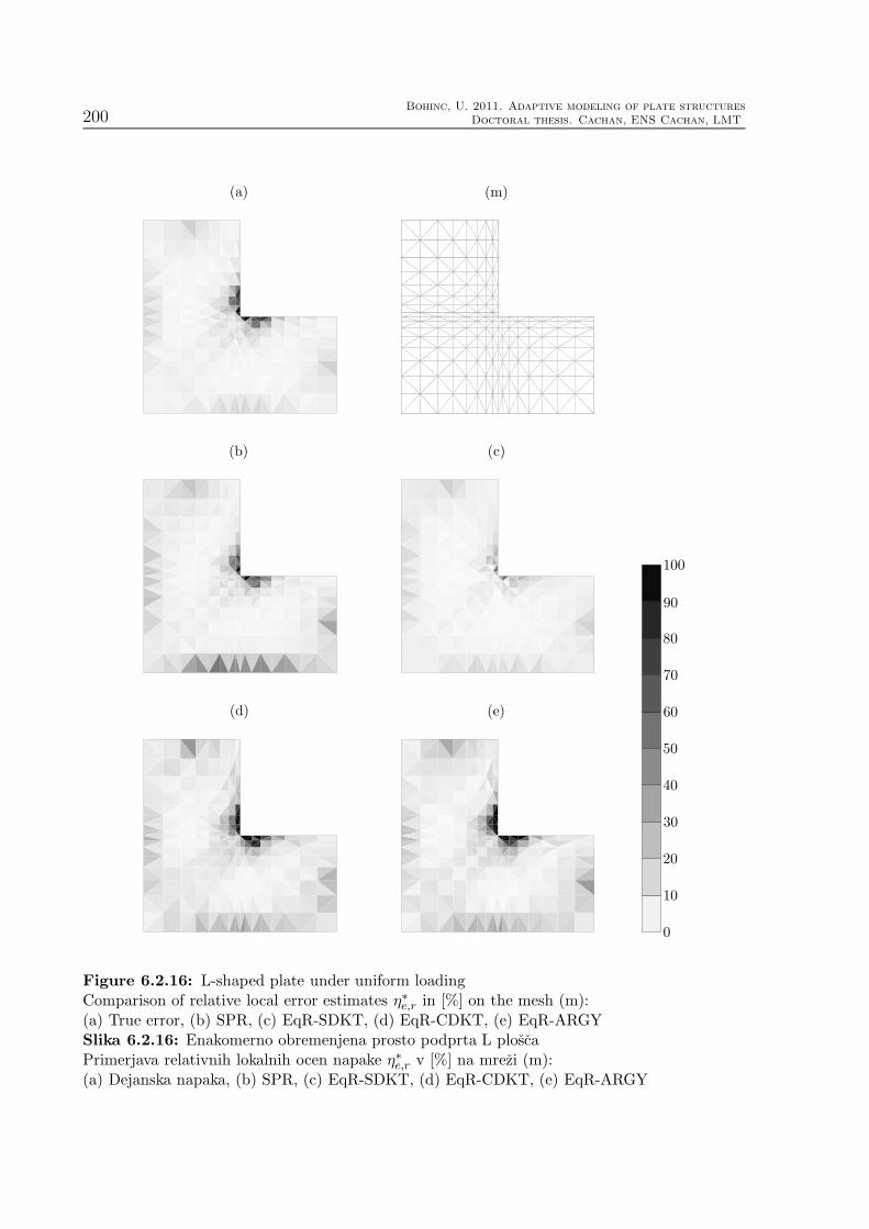
200Bohinc, U. 2011. Adaptive modeling of plate structures
Doctoral thesis. Cachan, ENS Cachan, LMT
(a) (m)
(b) (c)
(d) (e)
0
10
20
30
40
50
60
70
80
90
100
Figure 6.2.16: L-shaped plate under uniform loadingComparison of relative local error estimates η∗e,r in [%] on the mesh (m):(a) True error, (b) SPR, (c) EqR-SDKT, (d) EqR-CDKT, (e) EqR-ARGYSlika 6.2.16: Enakomerno obremenjena prosto podprta L ploscaPrimerjava relativnih lokalnih ocen napake η∗e,r v [%] na mrezi (m):(a) Dejanska napaka, (b) SPR, (c) EqR-SDKT, (d) EqR-CDKT, (e) EqR-ARGY

Bohinc, U. 2011. Prilagodljivo modeliranje ploskovnih konstrukcij
Doktorska disertacija. Ljubljana, UL, Fakulteta za gradbenistvo in geodezijo, Konstrukcijska smer 201
6.3 Discretization error for RM elements
RM plate elements, specifically the P3 elements introduced in Chapter 3, conform to the
same principles given above for the DK elements. The definition (5.3.4) of the local error
indicator is modified so, that it includes, besides the bending, also the shear deformation
energy:
η2e,RM =∑
e
∫
Ωeh
(m∗−mh)TC−1
B (m∗−mh) dΩ+∑
e
∫
Ωeh
(q∗−qh)TC−1
S (q∗−qh) dΩ (6.3.1)
SPR is method is applied in exactly the same manner as for the DK elements (practial
issues are discussed in [Lee Hobbs, 1998] and [Kettil Wiberg, 1999]). The application of
the EqR method to the P3 elements follows the same same steps as for the DK elements.
The reason for the similar treatment lies in the close similarity of the interpolations since
they are build on a hierarchic basis. Conceptually, the only novelty is the treatment of the
residuals to the midside degrees of freedom in P3 elements in the equilibration procedure.
It is apparent, that due to the simple topology, equilibration of the midside DOF is
not needed. Thus the equilibration procedures for DK and P3 elements are effectively
equal. The enhanced interpolations for the local computations are, however, limited to
the subdivision schemes, since there does not exist an enhanced P3 element (equivalent
to the ARGY element in the case of DK elements).
6.4 Chapter summary and conclusions
The focus of the chapter is the discretization error for the case of finite element Discrete
Kirchhoff plate model, which is widely accepted as finite element for the analysis of
bending of thin plates. Of particular challenge are the non-conventional finite element
interpolations for Discrete Kirchhoff plate bending elements. Hence, we can only provide
the error indicators (rather that rigorous error bounds), and even those require quite
ingenious procedures for constructing enhanced finite element space for error estimates.
The SPR method is nowadays widely accepted and found its way in many finite element
codes. The implementation for the Discrete Kirchhoff plate elements follows the general
principles of the method and it does not take into account the specific nature of the
problem. The EqR method, however, is significantly more difficult to implement, but it
has the potential of capturing specific issues related to modeling of plate bending. In this
work a special attention was given to the development of EqR method for this case.

202Bohinc, U. 2011. Adaptive modeling of plate structures
Doctoral thesis. Cachan, ENS Cachan, LMT
In particular, we have tested the equilibrated residual method with enhanced space
constructed by either subdividing the original element into 6 smaller elements (subdivision
into 3 smaller elements proved to be of no interest) or by using the Argyris plate element.
Although each of these enhanced elements possesses 21 degrees of freedom, they differ
in terms of providing the enhanced space. The former uses the patch like construction
with third order polynomials, whereas the latter uses the complete fifth order polynomial.
Thus, although both enhanced elements provide useful estimates, the latter, or the Argyris
element, furnishes superior results quality.

Bohinc, U. 2011. Prilagodljivo modeliranje ploskovnih konstrukcij
Doktorska disertacija. Ljubljana, UL, Fakulteta za gradbenistvo in geodezijo, Konstrukcijska smer 203
Chapter 7
Model error concept
7.1 Introduction
For the case of linear elasticity, which is the subject of this work, a complete and validated
three-dimensional theory exists, which captures all the physics of the deformation. In the
practical work in solid and structural mechanics, however, the theory is rarely applied.
The reason is, that for a given accuracy, the computational effort to obtain a solution is
exceptionally high. Simplified models were therefore developed which are valid only under
certain assumptions. The accuracy of this models is satisfactory for the most engineering
computations as long as the assumptions are satisfied.
Similar situation exists also in other areas. The motion of free falling body in the air,
for instance, is effectively computed using a Newton theory, rather than using quantum
theory, which is known to be more accurate. If the result of the computation is simply
a trajectory of the ball with a given accuracy, the Newton theory is obviously quite
adequate. For the practical use, the model must be computationally efficient while the
accuracy must match the prescribed one.
Engineering approach to modeling requires that the models are only as complex as
necessary. In the structural mechanics the need to develop the computationally effective
models is of particular importance. Several models of the typical structural members
were developed and tested which give accurate measurable predictions. They are based
on certain assumptions, which are typically satisfied in regular regions of a structure. In
the disturbed regions such as boundary layers, thickness jumps, stiffeners and regions with
concentrated loads enhanced models have to be used. Ultimately in the regions where none
of the assumptions apply a full three-dimensional theory of elasticity have to be employed.
Adaptive modeling in structural analysis has the goal to produce the most suitable (i.e.

204Bohinc, U. 2011. Adaptive modeling of plate structures
Doctoral thesis. Cachan, ENS Cachan, LMT
optimal) model of a structure. In order to construct a mixed - regionally adapted -
model, a sequence of hierarchically reduced, i.e. simplified, mathematical models derived
from an appropriate master model is required. The choice of particular model depends
on estimate of the model error. This information is the key to successful control of the
adaptive construction of the optimal model. The model error is related to the suitability
of model itself.
One should clearly distinguish between the model error estimates and model error
indicators. The estimates define the boundaries of the error. They are usually quite
conservative and they tend to overestimate the error by several orders of magnitude.
Indicators on the other hand do not provide any guarantees on the error. In return they
can give quite sharp indication of the error. Which type of model error to use depends
on the purpose of the computation of the model error. If the goal is to control the
adaptive construction of the optimal regional dependent model, the model indicators are
the preferable choice.
To locate regions of the domain where the chosen mathematical model (usually the
simplest one in a set of available hierarchic models) no longer performs well, one has to
provide an estimate of model performance. Ideally, such an estimate for the chosen model
should follow from the comparison with the best possible mathematical model (which
is often the 2D/3D solid model). However, the best model estimate is in general not
feasible, since it remains prohibitively expensive or simply inaccessible. Thus, for the
practical model error estimation, it is sufficient to compare the chosen model with the
one which is known to perform better; the latter will be called the enhanced model.
In principle, two global computations would be required to compare two different
mathematical models: the chosen against the enhanced one. However, the computations
with the enhanced model is usually simplified in trying to estimate the true stress state.
This is made possible by using the EqR method originaly developed for discretization
error estimation (see section 5.4.2). The procedure starts by extracting a portion of the
domain, reducing the computation to a single finite element based on the enhanced model,
applying the loading on its edges according to the true stress state estimate, computing
the local enhanced solution and comparing it to the original solution obtained by the
chosen model. This is of course possible only in principle, since the true stress state
is unknown. However, its approximation can be obtained by improving the FE solution
obtained with the chosen model to be best-possible approximation of the true stress state.
This is done as follows: the FE solution for any stress component (which is discontinuous

Bohinc, U. 2011. Prilagodljivo modeliranje ploskovnih konstrukcij
Doktorska disertacija. Ljubljana, UL, Fakulteta za gradbenistvo in geodezijo, Konstrukcijska smer 205
between the elements) is improved to be continuous in order to approximate the true stress
state, which is continuous (unless there is thickness, loading or material discontinuity). In
accordance with the best-possible approximation of the true stress state, the edge loading
(so-called boundary traction) for each finite element of the mesh is computed. That
loading is further used in computation of local (element-wise) Neumann problems based
on the enhanced model. Comparison of two mathematical models can be thus achieved
by one global and a set of local computations.
The effective procedure of computation od model error indicator is build upon the
following idea. The model error, in principle, measures the difference of the solutions of
the current and full three-dimensional model. Based on the assumption that the family
of models is hierarchically ordered, the model solution does not need to be compared to
the solution of the exact model. Due to the hierarchy, it suffices to compare the current
solution with the solution of the next model from the hierarchic family of models.
The global computation of the enhanced solution - just to serve as the reference to
model error computation - is too expensive. An effective compromise is to repeat the
computations with the enhanced model on smaller domains - preferably on elements.
The local problems have to replicate the original problem. The interpretation is, that
the elements are extracted from the continuum and its actions are replaced by boundary
tractions. The boundary conditions for the local problems are therefore of Neumann type.
7.2 Model error indicator based on local EqR com-
putations
7.2.1 Definition of model error indicator
The primary question of model error computation based on EqR method becomes: ”How
to estimate the boundary conditions for the local problems?”. If the enhanced solution is
known, the boundary conditions for the elements are computed from the stress state using
the Cauchy principle. This is, however, not possible since the stresses are computed from
the enhanced solution, which is unknown and yet to be computed. An approximation of
the boundary stresses must therefore be built based on the single information available:
current finite element solution. The development of the method of the construction of the
best possible estimates for the boundary conditions for local problems is thus the central
topic of the model error computation based on EqR method.
The enhanced solution, to which the original solution is compared to, is thus ap-

206Bohinc, U. 2011. Adaptive modeling of plate structures
Doctoral thesis. Cachan, ENS Cachan, LMT
proximated twice: (i) the boundary conditions for the local problems are computed only
approximately and (ii) the local problems are not solved exactly but rather in the weak
sense (finite element method) with the enhanced model. Such double approximation is
however still acceptable since the goal of the model error indicator is not to provide the
error bounds but to drive the model adaptivity procedure.
The starting point for the computation of the model error indicator is the finite element
solution of the problem using the coarse model - model 1. The finite element solution is
u1,h.
Let us suppose that the finite element solution u2,h using the enhanced model - model
2 - is available. Since the model error is of primary interest, let us assume also that the
discretization error is negligible or at least much smaller than the model error. In this case
the difference between the solutions can be entirely contributed to the model error. Since
the difference u2,h −u1,h is mathematically inconsistent, the difference of the solutions is
computed as:
eu,mod = u2,h − Pu,1→2u1,h
where Pu,1→2uh,1 denotes the kinematic transformation of the solution uh,1 to the solution
space of model 2.
Several measures of the difference of the solutions u2,h,uh,1 exist for the definition of
the model error indicator. The most straightforward is probably to use the energy norm
of eu,mod as the model error indicator
ηu,mod = ‖eu,mod‖E = ‖u2,h − Pu,1→2uh,1‖E
This definition of model error indicator is, however, prone to strong overestimation. An-
other option is to measure the model error in terms of the energy difference
ηu,mod = ‖u2,h‖E − ‖uh,1‖E
In most cases investigated this estimate is not sensitive enough, since the global energies
of the models 1 and 2 usually do not differ enough. In order to avoid the problems
mentioned, a model error is rather measured in terms of the stresses, i.e.:
eσ,mod = σ2,h − Pσ,1→2σh,1
The transformation Pσ,1→2σh,1 transforms the stresses from model 1 to model 2 using
the constitutive relation of model 2. Note, that eu,mod and eσ,mod are in different solution
spaces. The model error indicator is computed as the energy norm of eσ,mod:
ησ,mod = ‖eσ,mod‖E = ‖σ2,h − Pσ,1→2σh,1‖E

Bohinc, U. 2011. Prilagodljivo modeliranje ploskovnih konstrukcij
Doktorska disertacija. Ljubljana, UL, Fakulteta za gradbenistvo in geodezijo, Konstrukcijska smer 207
Ωeh
Γ Ω
Ωh
1
2
3
teΓe12
teΓe23
teΓe31
Ωeh
Figure 7.2.1: Local computation on a finite element domain Ωeh with Neumann boundary
conditions teΓe on Γe
Slika 7.2.1: Lokalni izracun s koncnimi elementi na obmocju Ωeh z Neumannovimi robnimi
pogoji teΓe on Γe
The complementary energy norm ‖ · ‖E is related to the model 2:
‖σ2‖2E =
∫
Ω
σ2 : C−22 : σ2dΩ
Construction of local problems
The model error can be estimated only via the comparison of the current solution with the
solution of the enhanced model. The global computation of the enhanced solution u2,h
is, however, not feasible. An alternative is the decomposition of the global problem into
smaller local problems. The local computations - preferably on elements - should ideally
give the same results as the global one. By a suitable choice of boundary conditions it is
possible in principle to define local problems with this property.
The finite element solution of the enhanced model 21, denoted by u2,h, satisfies the
weak form:
a2(u2,h, v2,h) = l2(v2,h); ∀v2,h ∈ V2,h (7.2.1)
The linear forms a2 and l2 refer to the model 2. The finite element solution space is
denoted by V2,h. The global problem can be replaced by a set of local problems, formed
1The subscript 2 will be related to the enhanced model.

208Bohinc, U. 2011. Adaptive modeling of plate structures
Doctoral thesis. Cachan, ENS Cachan, LMT
as:
a2,e(u2,e,h, v2,h) = l2,e(v2,h) +
∫
Γe
te2,Γe · v2,hds; ∀v2,h ∈ V2,h (7.2.2)
where the boundary conditions are of Neumann type. Along the boundary of the element,
denoted by Γe ≡ ∂Ωe, the element is loaded by boundary tractions te2,Γe . Boundary
tractions te2,ΓIJare undefined and are yet to be determined.
Additional condition for their construction comes from the observation, that the solu-
tion of the local problems should match the global finite element solution:
u2,e,h = u2,e,h (7.2.3)
The element solution u2,e,h = u2,h|Ωe is the restriction of the global finite element solution
to the element domain Ωe. Assuming that the global finite element solution u2,h is known,
the additional condition for the boundary tractions is:
∫
Γe
te2,Γe · v2,hds = a2,e(u2,e,h, v2,h)− l2,e(v2,h); ∀v2,h ∈ V2,h (7.2.4)
The symbolic form of the discretization of the j-th component of the test function v2,h
is (v2,h)j =∑
I NI2,j v2,I , where N
I2,j are the shape functions. Employing this notation, we
have for the integral over side ΓIJ :
∫
ΓIJ
te2,ΓIJ· v2,h du = re
2,I,ΓIJ· v2,I + re
2,J,ΓIJ· v2,J (7.2.5)
where the re2,I,ΓIJ
is the ‘projection’ of the boundary traction te2,ΓIJto the node I in the
finite element test space V2,h. We can interpret re2,I,ΓIJ
as residual forces at node I of
element e due to the boundary traction applied on edge ΓIJ , i.e.
re2,I,ΓIJ
=∂W e
ΓIJ(te2,ΓIJ
)
∂v2,I; W e
ΓIJ(te2,ΓIJ
) =
∫
ΓIJ
te2,ΓIJ· v2,hds (7.2.6)
From (7.2.4) the finite element equilibrium equation for a single element (7.2.4) can
be written also as
Re2 = Fint,e
2 − Fext,e2 (7.2.7)
where Fext,e2 , Re
2 and Fint,e2 are nodal values of external, residual and internal forces, respec-
tively. The later are proportional to the stiffness matrix Ke2 and the nodal displacements
ue2, so that (7.2.7) becomes:
Ke2u
e2 = Fext,e
2 +Re2
Residual forces Re2 represent the action of the surrounding elements.

Bohinc, U. 2011. Prilagodljivo modeliranje ploskovnih konstrukcij
Doktorska disertacija. Ljubljana, UL, Fakulteta za gradbenistvo in geodezijo, Konstrukcijska smer 209
The goal is to find such boundary traction forces that exactly replace the residual
forces and are continuous across element boundaries. We thus seek for boundary traction
teΓe acting on an edge Γe, which will replace (in an energy manner) the action of residual
nodal forces and reflect the continuity of the stress field. We can write
∑
I
Re2,I · v2,I =
∫
Γe
teΓe · v2,Γe,h ds =∑
ΓIJ
∫
ΓIJ
teΓIJ· v2,ΓIJ ,hds (7.2.8)
where v2,Γe = v2|Γe are edge virtual displacements, and v2,I are nodal virtual displace-
ments. The relation follows directly from (7.2.4):
a2,e(u2,e,h, v2,h)− l2,e(v2,h) =∑
I
Re2,I · v2,I (7.2.9)
where Re2,I is the nodal residual on node I of the element e. The vector of degrees of
freedom pertaining to the node I is denoted by v2,I .
From (7.2.5) we further express the nodal value of the element residual force Re2,I in
(7.2.8) as the sum (with slight abuse of the notation)
Re2,I = re
2,I,Γ1+ re
2,I,Γ2(7.2.10)
where Γ1 and Γ2 are two edges of element e that both include node I, see Figure 5.4.4.
Since the boundary tractions reflect the continuity of stress field, they conform to, see
Figure 5.4.3:
te2,ΓIJ+ te
′
2,ΓIJ= 0 (7.2.11)
Here the ΓIJ denotes the edge between the vertices I and J , adjacent to elements e and e′,
sharing the same edge ΓIJ . We note that the condition in (7.2.11) follows from te2,Γ = σne
and ne′ = −ne, where n is normal to the edge Γ and σ is continuous stress tensor. The
equation (7.2.11) is required to hold in the weak sense only:
∫
ΓIJ
(te2,ΓIJ+ te
′
2,ΓIJ) · v2,h ds = 0 (7.2.12)
re2,I,ΓIJ
+ re′
2,I,ΓIJ= 0
By collecting equations (7.2.10) and (7.2.11) for all elements in the mesh (e = 1, . . . , nel),
all element edges (ΓIJ = 1, . . . nΓ) and all element nodes (I = 1, . . . nen), we could get a
global system of equations for the unknowns re2,I,ΓIJ
(the number of unknowns in such a
system is reduced if there are regions of the discretized domain where boundary traction
forces are prescribed). Moreover, introduction of the projections re2,I,ΓIJ
as the unknowns,

210Bohinc, U. 2011. Adaptive modeling of plate structures
Doctoral thesis. Cachan, ENS Cachan, LMT
enables the formation of patchwise linear systems. For the patch of elements around node
I, we have (with sligh abuse of the notation):
re2,I,ΓIJ
+ re2,I,ΓIK
= Re2,I (7.2.13)
re2,I,ΓIJ
+ re′
2,I,ΓIJ= 0
where the only input (known) data are the element nodal reactions Re2,I . With a suitable
discretization, the boundary tractions are recovered from (7.2.5).
7.2.2 Construction of equilibrated boundary tractions for local
problems
The decomposition of the global problem as described above is possible only if the global
finite element solution u2,h is known in advance. In our case, the solution is yet to be
found and therefore the element nodal reactions Re2,I are unavailable for the computa-
tion. The boundary tractions te2,ΓIJ, which satisfy (7.2.13), cannot be computed and an
approximation have to be used. Note, however, that if the approximation for the bound-
ary tractions te2,ΓIJis used in the local problems (7.2.4), the solution u2,e,h of (7.2.2) no
longer matches the finite element solution u2,e,h.
The approximation of the boundary tractions te2,ΓIJmust meet some basic conditions.
First, the boundary tractions must maintain the element equilibrium. The element is in
equilibrium if the virtual work of the external forces vanishes at rigid body motion. Using
vΛ to denote rigid body motion, the condition for te2,Γe reads:∫
Γe
te2,Γe · vΛ = l2,e(vΛ); ∀vΛ ∈ VΛ ⊂ V2,h (7.2.14)
The boundary tractions satisfying (7.2.14) guarantee the element is in equilibrium. Sec-
ond, the global equilibrium of the assembly of elements is achieved if the boundary trac-
tions satisfy∫
ΓIJ
(te2,ΓIJ+ te
′
2,ΓIJ) · vΛ = 0; ∀vΛ ∈ VΛ ⊂ V2,h (7.2.15)
Although the two conditions (7.2.14) and (7.2.15) are necessary, they are quite general
and do not contribute to the any meaningful information about the problem in question.
Therefore, the third additional condition is set by specifying that the boundary traction
approximation should be chosen so, that the following holds:∫
Γe
te2,Γe · v1,hds = a1,e(u1,e,h, v1,h)− l1,e(v1,h); ∀v1,h ∈ V1,h (7.2.16)

Bohinc, U. 2011. Prilagodljivo modeliranje ploskovnih konstrukcij
Doktorska disertacija. Ljubljana, UL, Fakulteta za gradbenistvo in geodezijo, Konstrukcijska smer 211
In that case the solution of local problems u1,e,h
a1,e(u1,e,h, v1,h) = l1,e(v1,h) +
∫
Γe
te2,Γe · v1,hds; ∀v1,h ∈ V1,h (7.2.17)
match the original finite element solution u1,e,h = u1,e,h (obtained with the model 1).
Note, that, since VΛ ⊂ V1,h, the condition (7.2.14) is automatically satisfied.
The discretization of j-th component of v1,h is defined as (v1,h)j =∑
I NI1,j v
I1,j , which
gives:
∫
ΓIJ
te2,ΓIJ· v1,h du = re
21,I,ΓIJ· v1,I + re
21,J,ΓIJ· v1,J (7.2.18)
a1,e(u1,e,h, v1,h)− l1,e(v1,h) =∑
I
Re1,I · v1,I (7.2.19)
where the re21,I,ΓIJ
is the projection of the boundary traction te2,ΓIJto the node I in the
finite element test space V1,h. The element nodal reaction on node I on the element e
(model 1) is denoted as Re1,I .
The projections re21,I,ΓIJ
are the unknowns of the local patchwise systems - similar to
(7.2.13). For the patch of elements around node I we thus have
re21,I,ΓIJ
+ re21,I,ΓIK
= Re1,I (7.2.20)
re21,I,ΓIJ
+ re′
21,I,ΓIJ= 0
Example
In order to get further insight into the procedure of computation of boundary traction
projections, we inspect a patch of four 2D elements surrounding node I of the FE mesh
(see Figure 7.2.2). In this example the notation will be simplified so that the index
denoting the model will be dropped: Re1,I → Re
I , re21,I,Γ
→ reI,Γ. Edges and elements
are numbered in counter-clockwise manner. Application of equation (7.2.10) for this case
gives

212Bohinc, U. 2011. Adaptive modeling of plate structures
Doctoral thesis. Cachan, ENS Cachan, LMT
Re1I = re1
I,Γ4+ re1
I,Γ1
Re2I = re2
I,Γ1+ re2
I,Γ2
Re3I = re3
I,Γ2+ re3
I,Γ3
Re4I = re4
I,Γ3+ re4
I,Γ4
The demand for continuity fur-ther leads to
re1I,Γ1
+ re2I,Γ1
= 0
re2I,Γ2
+ re3I,Γ2
= 0
re3I,Γ3
+ re4I,Γ3
= 0
re4I,Γ4
+ re1I,Γ4
= 0
Γ1
Γ2
Γ3
Γ4I
e1 e2
e3e4
Figure 7.2.2: A patch of four elementssurrounding node I
Combination of the last two sets of equations leads to the following system
Re1I
Re2I
Re3I
Re4I
=
+1 0 0 −1−1 +1 0 00 −1 +1 00 0 −1 +1
re1I,Γ1
re2I,Γ2
re3I,Γ3
re4I,Γ4
(7.2.21)
for the unknowns rekI,Γk
. Since all the unknowns refer only to node I of the FE mesh, the
system is independent from other nodes. One thus obtains a local (patch-wise) problem;
a global system is actually a composition of independent patch-wise systems. If local
system (7.2.21) is solved for each node of the FE mesh, we obtain rekI,Γ, for all elements
of the mesh (ek = e = 1, . . . , nel), all element edges (Γ = 1, . . . nΓ) and all element nodes
(I = 1, . . . nen).
Recovery of boundary tractions from the projections
Result of the local patchwise computations are the projections re21,I,ΓIJ
for all nodes and
edges ΓIJ . Two projections exist for every edge ΓIJ : re21,I,ΓIJ
and re21,J,ΓIJ
. After a suit-
able discretization of te2,ΓIJis chosen, the boundary tractions are reconstructed using the
relation (7.2.18). The boundary tractions te2,ΓIJare consistent with model 2 and caution
should be taken when solving for te2,ΓIJ. The relation (7.2.18) namely assumes that the
boundary tractions conform to the kinematics of model 1.

Bohinc, U. 2011. Prilagodljivo modeliranje ploskovnih konstrukcij
Doktorska disertacija. Ljubljana, UL, Fakulteta za gradbenistvo in geodezijo, Konstrukcijska smer 213
Evaluation of boundary traction parameters from (7.2.18)
If reI,Γ are known2, the boundary traction can be computed for each element as follows.
We introduce parametrization of k-th component of the boundary traction teΓ (let Γ be
element edge between element nodes I and J) as
(teΓ)k = pIkψIk + pJkψ
Jk + pKk ψ
Kk (7.2.22)
where ψIk are shape functions (yet to be chosen) and pIk are nodal values of (teΓ)k. Here
we assumed, the edge has vertex nodes I and J and a midside node K. The variation of
virtual displacements along the same edge Γ can then be written as
(vΓ,h)k = N Ik,mv
Im +NJ
k,mvJm +NK
k,mvKm (7.2.23)
where vIm is the m-th degree of freedom at node I, and N Ik,m are the corresponding shape
functions. In other words, the shape function N Ik,i interpolates the k-th component of
virtual displacements vh,Γ and is weighted by nodal degree of freedom vi,I in the linear
interpolation (7.2.23). We can now insert the above parameterizations into (7.2.18) and
express residuals at nodes I and J with respect to the boundary traction on edge Γ (that
spans between I and J). The result can be written in a compact form as:
[reI,Γ
reJ,Γ
]=
[MII
Γ MIJΓ MIK
Γ
MJIΓ MJJ
Γ MJKΓ
]
pIΓ
pJΓ
pKΓ
; (7.2.24)
MIJΓ = [MI,J
Γ ]; MI,JΓ = [M I,J
Γ,nm]
where pIΓ =
[pIk, k = 1, . . . ndim
]T, and ndim is vector dimension. The block matrices MI,J
Γ
have nndofI rows and ndim columns with the elements
M I,JΓ,nm =
∫
Γ
N Im,nψ
Jmds (7.2.25)
The index m is denotes the virtual displacement component which is conjugated (in the
sense of the virtual work principle) to the traction component m.
By solving (7.2.25) for every element edge Γ, we obtain parameters pIΓ, which define
element boundary traction teΓ through (7.2.22).
It is suggested in the literature (e.g. [Ainsworth Oden, 2000], [Oden Cho, 1997]) that
shape functions ψJk and ψI
k should be such that MIJΓ and MJI
Γ vanish and the matrix M
2The subscript related to the model is dropped.

214Bohinc, U. 2011. Adaptive modeling of plate structures
Doctoral thesis. Cachan, ENS Cachan, LMT
becomes block diagonal. In such a case (7.2.25) simplifies to
reI,Γ = MII
Γ pIΓ (7.2.26)
This makes the bookkeeping for the computations much easier. However, our experience
is that the form of boundary traction obtained in this way is very specific and it does
not represent well the stress field. We also note that the specific choice of parametriza-
tion (7.2.26) is not necessary, since local patch-wise computation can be performed, see
(7.2.21).
Regularization of local system (7.2.21)
The solution of local system of equations, e.g. (7.2.21) for 2D problem, is not unique,
unless we impose an adequate additional regularization. The latter can be derived in
accordance with the estimate of the true stress state with the continuous boundary trac-
tion across the element interfaces. However, the true stress state is not known, but only
its (discontinuous) element-wise approximations σeFE obtained by model 1. Continuous
stresses at the edge Γ, denoted as σ0|Γ, follow from the smooth stress recovery which may
be coupled with previous mesh adaptivity procedure. Boundary traction forces resulting
from a such stresses σ0|Γ are obtained by the use of the Cauchy principle te,0Γ = σ0|Γne. It
is now possible to calculate the effect of this edge loading on neighboring nodes by using3
(7.2.6)
re,0I,Γ =
∂W eΓ(t
e,0Γ )
∂vI
(7.2.27)
We want reI,Γ to be as close as possible to this result in the least square sense. We construct
the following constrained patch-wise minimization problem:
LreI,Γ;λ
Γ; σe =1
2
∑
e∈PI
∑
Γ
(re,0I,Γ − re
I,Γ
)2
+∑
e∈PI
σeI(R
eI −
∑
Γ
reI,Γ)
+∑
Γ
λΓI (reI,Γ + re′
I,Γ) (7.2.28)
where the constraints (7.2.11) and (7.2.10) are also introduced by means of the corre-
sponding Lagrange multipliers σeI and λΓI , and PI is patch of elements around node I of
the FE mesh.
3The subscript related to the model is dropped again.

Bohinc, U. 2011. Prilagodljivo modeliranje ploskovnih konstrukcij
Doktorska disertacija. Ljubljana, UL, Fakulteta za gradbenistvo in geodezijo, Konstrukcijska smer 215
The Kuhn-Tucker optimality conditions for stationary point are then given by differ-
entiating the Lagrangian with respect to unknowns reI,Γ:
reI,Γ − r
e,0I,Γ − σe
I + λΓI = 0
The same equation also holds for the residual force on the neighboring element re′
I,Γ:
re′
I,Γ − re′,0I,Γ − σe′
I + λΓI = 0
If we sum up the last two equations and take into account the continuity condition
reI,Γ + re′
I,Γ = 0, we can express the Lagrange multiplier λΓI as
λΓI =1
2(σe
I + σe′
I + re,0I,Γ + r
e′,0I,Γ )
The unknowns reI,Γ can then be expressed in terms of the multiplier σe
I
reI,Γ =
1
2(σe
I − σe′
I + re,0I,Γ − r
e′,0I,Γ ) (7.2.29)
The condition reI = re
I,Γ1+ re
I,Γ2is rewritten as
reI =
1
2(re,0
I,Γ1− r
e1,0I,Γ1
) +1
2(re,0
I,Γ2− r
e2,0I,Γ2
) +1
2(σe
I − σe1I + σe
I − σe2I )
By exploiting the above results, the local system for the patch of four elements can be
rewritten as
Re1I
Re2I
Re3I
Re4I
=
1
2
2 −1 0 −1−1 2 −1 00 −1 2 −1−1 0 −1 2
σe1I
σe2I
σe3I
σe4I
(7.2.30)
where we introduced notation
ReI = Re
I −∑
Γ∈∂Ωe,I
< re,0I,Γ >; < r
e,0I,Γ >=
1
2(re,0
I,Γ − re′,0I,Γ )
The notation < · > implies averaging. The < re,0I,Γ > thus represent averaged boundary
traction on Γ (evaluated from FE solution) ’projected’ to node I.
To summarize, the element-wise boundary traction are computed from FE solution
(based on chosen mathematical model) in two steps: (i) by solutions of patch-wise prob-
lems in (7.2.30) to obtain reI,Γ; (ii) by solutions of element-wise problems (7.2.25) to
compute nodal values pIk of boundary tractions (7.2.22).

216Bohinc, U. 2011. Adaptive modeling of plate structures
Doctoral thesis. Cachan, ENS Cachan, LMT
Local problems as floating structures
The local problems (7.2.2) are of Neumann type. An element with only Neumman bound-
ary conditions is essentially a floating structure, and one thus ought to eliminate the rigid
body modes to get a unique result. This can be done simply by using the element geom-
etry, as shown in [Park Felippa, 1998]. A rigid body displacement deR of an element is a
linear combination of all its rigid body modes
deR = Deα (7.2.31)
where α is a vector of amplitudes that correspond to rigid body modes, and De is a
matrix containing the rigid body modes of the element (arranged column-wise). Since the
element stiffness matrix Ke is singular due to the rigid body modes contribution, one can
form a modified nonsingular stiffness matrix Ke by adding a product DeDeT to Ke
Ke = Ke +DeDeT
The inversion of K is possible and solution d (’rigid-body-polluted’ element nodal dis-
placements/rotations) can be obtained. Since the matrix DeDeT projects onto the space
spanned by rigid body modes, we have
d = de + deR
where de are real nodal displacements/rotations. As we are interested only in stress
resultants, such a ’pollution’ is not critical due to the following property KedeR = 0.
7.3 Chapter summary and conclusions
A general discussion of the model error estimation is given and a concept of hierarchi-
cally ordered models is introduced. Hierarchy of models enables computation of a model
estimate on the basis of the comparison of the results of two model computations: origi-
nal (model 1) and the enhanced one (model 2). Comparison of the results of two global
computations is clearly not rational. It is therefore desirable if the computation with the
enhanced model is done only locally - preferably on finite elements.
The local problems are of Neumann type - the boundaries are loaded with boundary
tractions representing the action of the surrounding continua. The central question of
model error estimation is: how to make an educated guess of the boundary tractions for
the local problems? The boundary tractions of the local problems are optimally computed
Bohinc, U. 2011. Prilagodljivo modeliranje ploskovnih konstrukcij
Doktorska disertacija. Ljubljana, UL, Fakulteta za gradbenistvo in geodezijo, Konstrukcijska smer 217
from the true stress state using the Cauchy principle. However, since the true stress
state is unknown, we seek for an alternative method for the computation of boundary
tractions. The alternative identified as useful is the method of equilibrated residuals
(EqR). The EqR method produces the boundary tractions, which exactly represent (in
the sense of principle of virtual work) the action of the element residual forces of the
original model (model 1). The basic principle of EqR method therefore coincides with
the concept of model error estimation. The second part of the chapter is thus devoted to
a general discussion of the computational aspects of EqR method related to the model
error computation.

218Bohinc, U. 2011. Adaptive modeling of plate structures
Doctoral thesis. Cachan, ENS Cachan, LMT

Bohinc, U. 2011. Prilagodljivo modeliranje ploskovnih konstrukcij
Doktorska disertacija. Ljubljana, UL, Fakulteta za gradbenistvo in geodezijo, Konstrukcijska smer 219
Chapter 8
Model error indicator for DKelements
8.1 Introduction
Analysis of plate structure with complex shape, loading and boundary conditions is one of
the most frequently encountered problems in structural engineering practice. A problem
of selecting the most suitable model for a particular plate structure, which is the topic of
this chapter, has therefore interesting practical aspects. If successfully solved, it can lead
to an efficient and accurate plate analysis, which is of great practical interest. Since plate
structures are often combined with frame and other skeletal structures, for which one can
develop by far the most efficient finite element analysis by exploiting one dimensional
form of the governing model and the superconvergence properties of the corresponding
finite element method, the solution of the above mentioned problem would clearly have a
very practical value.
Plates are basic structural elements and historically much attention has been given to
the derivation of different models. The derivation of the models has often been based on
various mechanical considerations and principles with no rigorous proof of the relationship
between the three-dimensional solution and the plate model. This kind of derivation has
also been used in this work (see chapters 2-4).
A sequence of plate models can be derived in an hierarchical way from three-dimensional
model. Using a model reduction a hierarchical sequence of elastic 2D plate models can be
be produced from 3D theory ([Babuska et al., 1983], [Szabo Sahrmann, 1988]). The mod-
els are controlled by two parameters p and q (p denotes the polynomial degree in terms of
standard plate coordinates, and q the polynomial degree in normal direction to the mid-
surface). Computable upper-bound error estimates are given by [Babuska Schwab, 1993],

220Bohinc, U. 2011. Adaptive modeling of plate structures
Doctoral thesis. Cachan, ENS Cachan, LMT
presuming that the resulting 2D PDEs (by reduction) are solved with prescribed error
tolerances. The plate modeling naturally can thus fit into the framework of hierarchic
modeling.
The hierarchic sequence of plate models can also be constructed with plate models,
based on the engineering insight as those presented in Chapters 2-4. Those models are
widely accepted in the practical computations since they are computationaly robust and
fast. In our work, we choose three plate models, which form a hierarchic family: the
Kirchhoff plate model (chapter 2), the Reissner/Mindlin plate model (chapter 3) and the
(1,1,2) plate model with through the thickness stretching (chapter 4).
An adaptive structural analysis of a plate structure as organized in our work starts
with a simplest possible plate model (Kirchhoff model). The model error with respect to
Reisnner/Mindlin model is computed and the regions where more refined model should
be used can be identified. The procedure can be iterated until the prescribed accuracy
is achieved throughout the problem domain by using the available models. An effective
computation of the model error is thus the key of the concept of adaptive modeling. The
above described procedure implies the need for a hierarchic family of plate models.
The model error indicator procedure described in chapter 7 will be specialized for plates
in this chapter. To construct the boundary stress resultants (which are plate counterparts
of solid boundary traction) we follow the procedure outlined e.g in [Ladeveze Leguillon,
1983], [Ladeveze Maunder, 1996], [Stein Ohnimus, 1997], [Oden Cho, 1997] for 3D
elasticity and briefly presented in chapter 7. The local problem that needs to be solved
(to get a model error indicator/estimate) deals with single plate element, which is floating
structure, loaded on the surface and along its edges in such a way that the loads are self-
equilibrated. We can thus speak about the model adaptivity procedure for plates that is
based on equilibrated boundary stress resultants1.
Due to the hybrid construction of the DK plate elements, the standard computation of
equilibrated boundary tractions is modified. The detailed procedure for the computation
of the boundary tractions of the local problems will be given in the following (see also
[Bohinc et al., 2006], [Bohinc et al., 2009]).
1We will not distinguish between boundary stress resultants and boundary tractions in what follows

Bohinc, U. 2011. Prilagodljivo modeliranje ploskovnih konstrukcij
Doktorska disertacija. Ljubljana, UL, Fakulteta za gradbenistvo in geodezijo, Konstrukcijska smer 221
8.2 Model error indicator
In order to find equilibrated stress resultants for the DK plate elements, we start with
interpolations for displacement and rotations. The displacement along the element bound-
ary ΓIJ , spanned between the element nodes I and J , is defined (according to (2.3.59))
by:
wh,ΓIJ= wI ϕ1 + wJ ϕ2 +
LIJ
4nIJ · (θI − θJ) ϕ3 +
LIJ
3∆θIJ ϕ4 (8.2.1)
where ∆θIJ = 32 LIJ
(wJ − wI) − 34nIJ · (θI + θJ), LIJ is the length of the edge ΓIJ and
nIJ = [nx,IJ , ny,IJ ]T is the unit exterior normal. Similarly, rotation vector along the same
edge is defined as
θh,ΓIJ= θI ϕ1 + θJ ϕ2 + nIJ∆θIJ ϕ3 (8.2.2)
The shape functions ϕi in (6.2.2) and (6.2.3) are:
ϕ1 = (1− ξ)/2 ϕ2 = (1 + ξ)/2 (8.2.3)
ϕ3 = (1− ξ2)/2 ϕ4 = ξ(1− ξ2)/2,
where ξ ∈ [−1, 1]. In accordance with (8.2.1), (8.2.2) and notation used in (7.2.23),
one can write the interpolation functions. For displacement or rotations on the edge Γ
(between vertex nodes I and J) as
N Iw,w = ϕ1 − ϕ4/2 NJ
w,w = ϕ2 + ϕ4/2 (8.2.4)
N Iw,θx
= −Lnx(−ϕ3 + ϕ4)/2 NJw,θx
= −Lnx(+ϕ3 + ϕ4)/2
N Iw,θy
= −Lny(−ϕ3 + ϕ4)/2 NJw,θy
= −Lny(+ϕ3 + ϕ4)/2
N Iθx,w = +(3nx/L)ϕ3 NJ
θx,w = −(3nx/L)ϕ3
N Iθx,θx
= ϕ1 + 3n2xϕ3/2 NJ
θx,θx= ϕ2 + 3n2
xϕ3/2
N Imxθy = +3nxnyϕ3/2 NJ
θx,θy= +3nxnyϕ3/2
N Iθy ,w = +(3ny/L)ϕ3 NJ
θy ,w = −(3ny/L)ϕ3
N Iθy ,θx
= +3nxnyϕ3/2 NJθy,θx
= +3nxnyϕ3/2
N Iθy ,θy
= ϕ1 + 3n2yϕ3/2 NJ
θy ,θy= ϕ2 + 3n2
yϕ3/2
where L = LIJ , nIJ = [nx, ny], θx = θ1 and θy = θ2. Note, that with respect to (7.2.23)
and notation in previous chapter one has: k ∈ [w, θx, θy], m ∈ [w, θx, θy] and
(vΓ,h)w = wh,Γ, (vΓ,h)θx = θxh,Γ, (vΓ,h)θy = θyh,Γ

222Bohinc, U. 2011. Adaptive modeling of plate structures
Doctoral thesis. Cachan, ENS Cachan, LMT
The boundary stress resultant vector for the DK plate element at the edge Γ has three
components
teΓ = [q,ms, mn] (8.2.5)
where q is the shear force along the edge defined in direction of z-axis, and mn, ms are
the moments defined in the direction normal to the element side and along the element
side, respectively. We choose to parameterize2 them as
qΓ = qK,Γ (8.2.6)
ms,Γ = msI,Γϕ1 +msJ,Γϕ2
mn,Γ = mnI,Γϕ1 +mnJ,Γϕ2 +mnK,Γϕ3
With respect to the notation introduced in (5.4.41), we note that
ψIk = ϕ1 ψJ
k = ϕ2 ψKk = ϕ3 (8.2.7)
and
pIq = 0 pJq = 0 pKq = qK,Γ (8.2.8)
pIms= msI,Γ pJms
= msJ,Γ pKms= 0 (8.2.9)
pImn= mnI,Γ pJmn
= mnJ,Γ pKmn= mnK,Γ (8.2.10)
(8.2.11)
To get the nodal parameters of (8.2.6) from (7.2.25) we have to evaluate integrals
M IJΓ,nm =
∫ΓN I
m,nψJmds, elements of block matrix MIJ
Γ
MIJΓ =
L
2
∫ +1
−1
N Iw,wψ
Jq N I
θs,wψJms
N Iθn,w
ψJmn
N Iw,θx
ψJq N I
θs,θxψJms
N Iθn,θx
ψJmn
N Iw,θy
ψJq N I
θs,θyψJms
N Iθn,θy
ψJmn
dξ (8.2.12)
where the following transformation was used:
Nθs,· = −nyNθx,· + nxNθy,· (8.2.13)
Nθn,· = +nxNθx,· + nyNθy ,·
with (·) standing for w, θx and θy.
2The parametrization is arbitrary, however, the total number of free parameters must not exceed the
number of components of input data reI,Γ

Bohinc, U. 2011. Prilagodljivo modeliranje ploskovnih konstrukcij
Doktorska disertacija. Ljubljana, UL, Fakulteta za gradbenistvo in geodezijo, Konstrukcijska smer 223
The boundary tractions projections reI,Γ = [rwI,Γ, rθxI,Γ, r
θyI,Γ] are computed from the patch-
wise local systems of equations (7.2.30). The parameters for (8.2.6) are computed form
the inverse of the system (7.2.25). We obtain:
qKΓ =rwI,Γ + rwJ,Γ
L(8.2.14)
mIs,Γ =
2ny(+rθxJ,Γ − 2rθxI,Γ) + 2nx(+2r
θyI,Γ − r
θyJ,Γ)
L
mJs,Γ =
2ny(+rθxI,Γ − 2rθxJ,Γ) + 2nx(+2r
θyJ,Γ − r
θyI,Γ)
L
mIn,Γ =
ny(+33rθyI,Γ + 21r
θyJ,Γ) + nx(+33rθxI,Γ + 21r
θyJ,Γ)
2L− rwI,Γ
mJn,Γ =
ny(+33rθyJ,Γ + 21r
θyI,Γ) + nx(+33rθxJ,Γ + 21r
θyI,Γ)
2L+ rwI,Γ
mKn,Γ =
15(nx(rθxI,Γ + rθxJ,Γ) + ny(r
θyI,Γ + r
θyJ,Γ))
L
8.2.1 Regularization
To form the minimization function (7.2.28), the projections re,0I,Γ are required. They are
computed from the improved approximation of the boundary traction te,0Γ = [q0, m0
s, m0n].
If the improved boundary tractions are expressed in the form (7.2.22), the projections are
computed using the equation (7.2.25).
The boundary traction approximation te,0Γ is computed from the current finite element
solution using the following technique: edge boundary traction t0Γ is taken as an average
of the boundary tractions te,0Γ and t
e′,0Γ computed from the stress resultants of the two
elements e and e′ adjacent to the edge Γ:
t0Γ = (te,0Γ − te′,0Γ )/2 (8.2.15)
Boundary tractions te,0Γ are evaluated at side Γ from element stress resultants from
the Cauchy principle. First, the stress resultants at the integration points mh(ξgp) =
CBκh(ξgp) are evaluated. A linear interpolation of the stress resultants
m0 =∑
I
m0INI (8.2.16)
is constructed using the least squares fit to mh(ξgp). At the element side Γ, defined by

224Bohinc, U. 2011. Adaptive modeling of plate structures
Doctoral thesis. Cachan, ENS Cachan, LMT
unit exterior normal n = [nx, ny]T , we thus have:
m0n = (m0
yy −m0xx)nxny +m0
xy(n2x − n2
y) (8.2.17)
m0s = (m0
xxn2x +m0
yyn2y + 2m0
xynxny)
The shear component normal to the edge is obtained from
q0 = q0xnx + q0yny
where the components q0x, q0y are computed from equilibrium equations:
q0x = −(∂m0
xx
∂x+∂m0
xy
∂y); q0y = −(
∂m0yy
∂y+∂m0
xy
∂x) (8.2.18)
The effective shear q0ef however is computed from q0ef = q0 − ∂m0n
∂sand the derivative ∂m0
n
∂s
is evaluated from (8.2.17) using the interpolation (8.2.16).
Model error indicator for the DK plate elements is obtained by comparing its results
with the ones obtained by an element based on more refined plate model RM. As shown
above, the later results can be obtained by element-wise computation with the DK bound-
ary stress resultants applied as external edge loading. Thus, a Neumann-type problem
has to be solved for each element of the mesh.
8.2.2 The local problems with RM plate element
The local problems are written as
Ke2u
e2 = Fext,e
2 +Re2 (8.2.19)
where Ke2 is the RM element stiffness matrix, Fext,e
2 is the external load vector contributed
to surface load and Re2 are the element nodal residuals due to external edge load. The ex-
ternal load vector Re2 = [Re
2,I , · · · ,Re2,IJ , · · · ]T corresponding to the external edge loading
is computed from
∑
I
Re2,I · ve
2,I +∑
IJ
Re2,IJ · ve
2,IJ =
∫
Γe
teΓe · v2,Γe,h ds =∑
ΓIJ
∫
ΓIJ
teΓIJ· v2,ΓIJ ,hds (8.2.20)
where ve2 = [ve
2,I , · · · , ve2,IJ , · · · ]T . The element edge load te2,ΓIJ
= [qΓIJ, ms,ΓIJ
, mn,ΓIJ]T is
defined by (8.2.14) and (8.2.6). We have
∫
Γe
te2,ΓIJ· ve
2,ΓIJ ,hds =
∫
Γe
(qvRMh +msϑ
RMs,h +mnϑ
RMn,h ) ds (8.2.21)

Bohinc, U. 2011. Prilagodljivo modeliranje ploskovnih konstrukcij
Doktorska disertacija. Ljubljana, UL, Fakulteta za gradbenistvo in geodezijo, Konstrukcijska smer 225
where the virtual displacements ve2,h = [vRM
h , ϑRMs,h , ϑ
RMn,h ]
T are those of RM element.
The interpolation of the RM plate elements is an hierarchic extension of the interpo-
lation of the DK element:
vRMh = vDK
h −∑
IJ
L
4γIJMIJ
ϑRMh = ϑDK
h +∑
IJ
3
2nIJ γIJNIJ
With respect to the DK plate elements, RM plate elements have an additional degree of
freedom ve2,IJ = [γIJ ] on the midside of the element edges (Re
2,IJ = [Re2,IJ ]). The nodal
degrees of freedom are the same for both elements ve2,I = ve
1,I .
On the edge ΓIJ we have:
vRMΓIJ ,h
= vDKΓIJ ,h
− 1
2LIJ γIJϕ4; ϑRM
s,ΓIJ ,h= ϑDK
s,ΓIJ ,h; ϑRM
n,ΓIJ ,h= ϑDK
n,ΓIJ ,h− 3γIJϕ3
which leads to:
∑
ΓIJ
∫
ΓIJ
(qvRMh +msϑ
RMs,h +mnϑ
RMn,h )ds = (8.2.22)
∑
ΓIJ
∫
ΓIJ
(qvDKh +msϑ
DKs,h +mnϑ
DKn,h )ds−
∑
ΓIJ
γIJ
∫
ΓIJ
(LIJ
2q ϕ4 + 3mn ϕ3
)ds
Since
∑
ΓIJ
∫
ΓIJ
(qvDKh +msϑ
DKs,h +mnϑ
DKn,h )ds =
∑
I
Re1,Iv
e1,I (8.2.23)
we realize from (8.2.22), that the following holds:
Re2,I = Re
1,I ; (8.2.24)
Re2,IJ =
∫
Γe
(LIJ
2q ϕ4 + 3mn ϕ3
)ds
The element nodal residuals of the RM element are the same as those of DK element,
except for the element residuals corresponding to the midside degrees of freedom. The
equilibration procedure does not influence the element nodal residuals Re2,I . However, the
equilibration is still necessary, since it determines the edge loading q and mn, which define
the load vector Re2,IJ through (8.2.24). By taking the values for q and mn from (8.2.14)
and (8.2.6) we have
Re2,IJ =
LIJ
2(rqJ,ΓIJ
− rqI,ΓIJ) (8.2.25)

226Bohinc, U. 2011. Adaptive modeling of plate structures
Doctoral thesis. Cachan, ENS Cachan, LMT
8.2.3 Computation of the model error indicator
Having defined the stress resultants for the RM, the RM deformation energy can be
calculated, by taking into account the corresponding bending and shear deformations
ERM,e =
∫ e
Ω
mRM,T CB−1mRM dΩ +
∫ e
Ω
qRM,T CS−1qRM dΩ
= ERM,B
e+ ERM,
S
e(8.2.26)
where mRM = [mxx, myy, mxy]T and qRM = [qx, qy]
T .
Since DK and RM plate elements predict very similar values for moments and the
DK assumes zero shear strains, the shear deformation energy ERM,S
eof RM can be used
to determine how well the DK plate model performs in a given situation. If shear strain
contribution is low enough, the DK could be considered as a sufficiently good model,
otherwise it should be replaced by a more suitable element based on Reissner/Mindlin
model (i.e. by the RM plate element). A fairly reasonable choice for a model error
indicator ηMe we use herein is therefore the ratio of the energy norm of the shear difference
between the RM and the DK element to the total energy of the RM element. Due to
the zero shear strain assumption in the DK, and similar prediction for moments of both
elements, one can define the model error indicator as
ηMe = ERMS
,e/ERM,e (8.2.27)
This indicator is used below in all numerical examples.
8.2.4 Numerical examples
We present in this section results of numerical examples, which were chosen to illustrate
performance of the proposed approach to adaptive modeling of plates. The departure
point for the present model adaptivity procedure should be an optimally adapted FE mesh,
with the discretization error uniformly distributed and placed within a predefined limit.
We note that the plate elements in such an automatically generated mesh of quadrilaterals,
which takes into account predefined element size distribution, can be quite distorted. For
this reason we also present examples where the influence of mesh distortion on the chosen
model error indicator is studied.
Simply supported square plate
Problem of simply supported (SSSS) square plate under uniform loading is used to test
the sensitivity of model error indicator on mesh distortion; as well as to compare those

Bohinc, U. 2011. Prilagodljivo modeliranje ploskovnih konstrukcij
Doktorska disertacija. Ljubljana, UL, Fakulteta za gradbenistvo in geodezijo, Konstrukcijska smer 227
effects for thin and thick plate situations. The material is linear elastic and isotropic, with
Young’s modulus E = 10.92 and Poisson’s ratio ν = 0.3. The side length is a = 10. Two
values for the plate thickness t = 0.1 (thin) and t = 1 (thick) are selected. Due to the
symmetry, only one quarter of the plate (the lower left one) is chosen for the numerical
analysis.
The model error indicator (8.2.27) is computed for each DKQ element of the mesh.
This value is then compared with the corresponding analytical (reference) value, which
can be for this simple problem obtained by using analytical (series) solution for Mindlin
plates, see e.g. [Lee et al., 2002], [Brank, 2008]. In Figure 8.2.1, we show the comparison
of two structured (regular) meshes with the same number of elements for the case of thick
plate. The meshes differ in discretization error, which is lower for the second mesh that
is more refined towards the outer edges. It can be observed that the computed model
error indicator is very close to the reference one, except for the corner element. This is
due to the fact that the equilibration is not possible to carry out at the corner node. We
thus obtain as a consequence that the estimated boundary stress resultants for the corner
element are not as good as for the inner elements.
To estimate the effect of mesh distortion, the model error indicator (8.2.27) is com-
puted (for the case of thick plate) with two distorted meshes. The first mesh is obtained
by adaptive mesh refinement with 5% tolerance in discretization error. The second one is
derived from the mesh shown in Figure 8.2.1 by a parametrical displacement of the nodes.
The results are presented in Figure 8.2.2. Again, comparison is made with the analytical
(reference) solution. We note that the performance of model error indicator is slightly
better for parametrical distortion of the mesh. One may conclude from the results shown
in Figure 8.2.2 that the model error indicator is slightly (but not severely) influenced by
mesh distortion.
We repeat the above mentioned comparison also for the case of thin plate. The result
are shown in Figure 8.2.3 and 8.2.4 (notice the change of scale). The model error indicator
shows that the DKQ is sufficiently good (almost) for the whole mesh. Comparison with
the analytical solution shows that the sensitivity of model error indicator is of the same
range as in the case of thick plate.
Square plate with two simply supported and two free edges
The second problem we study is a square plate with two opposite edges simply supported
and two other edges free (SFSF). It has been chosen to test the ability of the proposed

228Bohinc, U. 2011. Adaptive modeling of plate structures
Doctoral thesis. Cachan, ENS Cachan, LMT
30.0
20.0
10.0
0.0
(b)
[%]
100.0
90.0
80.0
70.0
60.0
50.0
40.0
(a)
30.0
20.0
10.0
0.0
(b)
[%]
100.0
90.0
80.0
70.0
60.0
50.0
40.0
(a)
Figure 8.2.1: Reference value of model error indicator (a) and its estimated value (b) for thickSSSS plate for rectangular meshesSlika 8.2.1: Referencna vrednost modelske napake (a) ter njena ocena (b) za srednje debeloSSSS plosco s pravokotno mrezo
procedure to detect boundary layer effect, which is most prominent along the free edges,
see [Arnold Falk, 1989]. The width of the boundary layer is proportional to the thickness
of the plate, and it is most pronounced for the transverse shear component, which varies
as 1/t. The geometry and material parameters are the same as in the first example. Due
to the symmetry, only one quarter of the plate (the lower left one) is used in the analysis;
the boundary conditions are imposed as follows: the left edge in simply supported, the
lower one is free, and the right and the upper ones take into account symmetry.
Since the boundary layer effect is intrinsic to the Reissner/Mindlin theory, the DKQ
can not detect it. In the present procedure the equilibrated boundary stress resultants
are derived from the DKQ solution and subsequently applied to the P3Q in order to
evaluate model error indicator. It is therefore interesting to see weather this procedure
can effectively detect the boundary layer. The result shown in Figure 8.2.5 indicates that
the procedure is able to detect a region with increased shear deformation energy (along

Bohinc, U. 2011. Prilagodljivo modeliranje ploskovnih konstrukcij
Doktorska disertacija. Ljubljana, UL, Fakulteta za gradbenistvo in geodezijo, Konstrukcijska smer 229
60.0
50.0
40.0
30.0
20.0
10.0
0.0
(b)
[%]
100.0
90.0
80.0
70.0
(a)
30.0
20.0
10.0
0.0
(b)
[%]
100.0
90.0
80.0
70.0
60.0
50.0
40.0
(a)
Figure 8.2.2: Reference value of model error indicator (a) and its estimated value (b) for thickSSSS plate for distorted meshesSlika 8.2.2: Referencna vrednost modelske napake (a) ter njena ocena (b) za srednje debeloSSSS plosco z deformirano mrezo
the left edge) but is not very successful to detect the boundary layer (along the lower free
edge), which is clearly observable in the reference (analytical) solution. Comparison with
the analytical solution shows (see Figures 8.2.5, 8.2.6, 8.2.7 and 8.2.8) that the sensitivity
of model error indicator is of the same range as in the case of SSSS plate.
Adaptive analysis of L-shaped plate
Adaptive model analysis of an L-shaped plate under uniform unit pressure is considered
in this example. Long sides (a = 10) of the plate are clamped, all other sides (b = 5)
are free. The plate is made of linear elastic isotropic material, with Young’s modulus
E = 10.92 and Poisson’s ratio ν = 0.3. Thickness of the plate is equal to 1. Non distorted
mesh was chosen for this example in order to avoid effect of element distortion on model
error indicator.

230Bohinc, U. 2011. Adaptive modeling of plate structures
Doctoral thesis. Cachan, ENS Cachan, LMT
1.5
1.0
0.5
0.0
(b)
[%]
5.0
4.5
4.0
3.5
3.0
2.5
2.0
(a)
1.5
1.0
0.5
0.0
(b)
[%]
5.0
4.5
4.0
3.5
3.0
2.5
2.0
(a)
Figure 8.2.3: Reference value of model error indicator (a) and its estimated value (b) for thinSSSS plate for rectangular meshesSlika 8.2.3: Referencna vrednost modelske napake (a) ter njena ocena (b) za tanko SSSS ploscos pravokotno mrezo
The computation started with the analysis of the plate by using DKQ elements. The
model error indicator (8.2.27) was further computed and the result is shown in Fig-
ure 8.2.9. The indicator identified several regions where the model error was high. The
limit of 15% model error was chosen to determine the elements of the mesh, where the
P3Q should be used instead of the DKQ. Those elements are colored dark grey in Fig-
ures 8.2.10-8.2.12 (b). Finally, the computation with both the DKQ (light grey in Fig-
ures 8.2.10-8.2.12 (b)) and the P3Q elements (dark grey in Figures 8.2.10-8.2.12 (b)), used
at different regions of the plate, was performed. Kinematic coupling of elements based on
different models was considered, i.e. the hierarchic rotation ∆θ of the P3Q was restrained
on edges where the P3Q elements were adjacent to the DKQ elements in order to account
for zero transverse shear modelling along those edges.
The comparison of stress resultants evaluated with the DKQ elements (Figures 8.2.10-
8.2.12 (a)), with the P3Q elements (Figures 8.2.10-8.2.12 (c)) and with both the DKQ

Bohinc, U. 2011. Prilagodljivo modeliranje ploskovnih konstrukcij
Doktorska disertacija. Ljubljana, UL, Fakulteta za gradbenistvo in geodezijo, Konstrukcijska smer 231
3.0
2.5
2.0
1.5
1.0
0.5
0.0
(b)
[%]
5.0
4.5
4.0
3.5
(a)
1.5
1.0
0.5
0.0
(b)
[%]
5.0
4.5
4.0
3.5
3.0
2.5
2.0
(a)
Figure 8.2.4: Reference value of model error indicator (a) and its estimated value (b) for thinSSSS plate for distorted meshesSlika 8.2.4: Referencna vrednost modelske napake (a) ter njena ocena (b) za tanko SSSS ploscoz deformirano mrezo
and the P3Q elements (Figures 8.2.10-8.2.12 (d)) is shown. It can be seen that the
P3Q based computation and the mixed DKQ-P3Q based computation produce almost
identical results; on the other hand, the results are not equal to those obtained by using
only DKQ elements. Therefore, the comparison of these different results (and especially
close agreement between the DKQ-P3Q and the P3Q computations), clearly indicates
that the adaptive procedure of this kind performs successfully. One can hope for the
same trend when applying the same procedure to higher order plate models, where a
significant computational savings could also be obtained in the process.
Adaptive analysis of Morley’s skew plate
Adaptive model analysis of Morley’s 30 skew plate (see [Morley, 1963]) with thickness t =
1, side length a = 10, simple supports on all sides, and unit uniform pressure is performed

232Bohinc, U. 2011. Adaptive modeling of plate structures
Doctoral thesis. Cachan, ENS Cachan, LMT
30.0
20.0
10.0
0.0
(b)
[%]
100.0
90.0
80.0
70.0
60.0
50.0
40.0
(a)
30.0
20.0
10.0
0.0
(b)
[%]
100.0
90.0
80.0
70.0
60.0
50.0
40.0
(a)
Figure 8.2.5: Reference value of model error indicator (a) and its estimated value (b) for thickSFSF plate for rectangular meshesSlika 8.2.5: Referencna vrednost modelske napake (a) ter njena ocena (b) za debelo SFSFplosco s pravokotno mrezo
in this example. The plate is built of linear elastic isotropic material, with Young’s
modulus E = 10.92 and Poisson’s ratio ν = 0.3. The most interesting feature of the
solution to this problem concerns two singular points at the two obtuse corners of the plate,
which strongly influence the quality of the computed results (e.g. see [Ibrahimbegovic,
1993]). The chosen FE mesh is made more dense near the sides of the plate where
singularities are expected.
The computation started with the analysis by using DKQ elements. The model error
indicator (8.2.27) was further computed, see Figure 8.2.13. It can be seen from Fig-
ure 8.2.13 that the error was increased near the sides and in the vicinity of the obtuse
corners. Again, the limit of 15% model error was chosen to determine the elements of the
mesh, where the P3Q should be used instead of the DKQ; all such elements are colored
dark grey in (b) part of Figures 8.2.14 and 8.2.15. Finally, the computation with both
the DKQ (light grey in Figures 8.2.14(b) and 8.2.15(b)) and the P3Q elements (dark grey

Bohinc, U. 2011. Prilagodljivo modeliranje ploskovnih konstrukcij
Doktorska disertacija. Ljubljana, UL, Fakulteta za gradbenistvo in geodezijo, Konstrukcijska smer 233
90.0
80.0
70.0
60.0
50.0
40.0
30.0
20.0
10.0
0.0
(b)
[%]
100.0
(a)
30.0
20.0
10.0
0.0
(b)
[%]
100.0
90.0
80.0
70.0
60.0
50.0
40.0
(a)
Figure 8.2.6: Reference value of model error indicator (a) and its estimated value (b) for thickSFSF plate for distorted meshesSlika 8.2.6: Referencna vrednost modelske napake (a) ter njena ocena (b) za debelo SFSFplosco z deformirano mrezo
in Figures 8.2.14-8.2.15 (b)), used at different regions of the plate, was performed.
It can be seen in Figure 8.2.14 that in this case the difference in results for moments
between all three computational models is negligible. The difference however still shows
in the results for the shear force, which are presented in Figure 8.2.16.

234Bohinc, U. 2011. Adaptive modeling of plate structures
Doctoral thesis. Cachan, ENS Cachan, LMT
1.5
1.0
0.5
0.0
(b)
[%]
5.0
4.5
4.0
3.5
3.0
2.5
2.0
(a)
1.5
1.0
0.5
0.0
(b)
[%]
5.0
4.5
4.0
3.5
3.0
2.5
2.0
(a)
Figure 8.2.7: Reference value of model error indicator (a) and its estimated value (b) for thinSFSF plate for rectangular meshesSlika 8.2.7: Referencna vrednost modelske napake (a) ter njena ocena (b) za tanko SFSF ploscos pravokotno mrezo

Bohinc, U. 2011. Prilagodljivo modeliranje ploskovnih konstrukcij
Doktorska disertacija. Ljubljana, UL, Fakulteta za gradbenistvo in geodezijo, Konstrukcijska smer 235
4.5
4.0
3.5
3.0
2.5
2.0
1.5
1.0
0.5
0.0
(b)
[%]
5.0
(a)
1.5
1.0
0.5
0.0
(b)
[%]
5.0
4.5
4.0
3.5
3.0
2.5
2.0
(a)
Figure 8.2.8: Reference value of model error indicator (a) and its estimated value (b) for thinSFSF plate for distorted meshesSlika 8.2.8: Referencna vrednost modelske napake (a) ter njena ocena (b) za tanko SFSF ploscoz deformirano mrezo
50
40
30
20
10
[%]
100
0
90
70
60
80
Figure 8.2.9: Model error indicator for LSHP problemSlika 8.2.9: Ocena modelske napake za primer LSHP

236Bohinc, U. 2011. Adaptive modeling of plate structures
Doctoral thesis. Cachan, ENS Cachan, LMT
11.70
10.16
8.61
7.07
5.52
3.98
2.43
0.89
-0.66
-2.20
-3.75(d)(c)
(b)
11.70
(a)
Figure 8.2.10: Stress resultant mxx (a) DKQ, (c) P3Q and (d) DKQ-P3Q model. The mod-elisation of (d) is presented in (b), where dark areas represent P3Q and light ones DKQ model.Slika 8.2.10: Rezultante napetosti mxx (a) DKQ, (c) P3Q in (d) DKQ-P3Q model. Mesanmodel (d) je predstavljen v (b), kjer temnejsa podrocja prikazujejo P3Q in svetlejsa DKQ model.
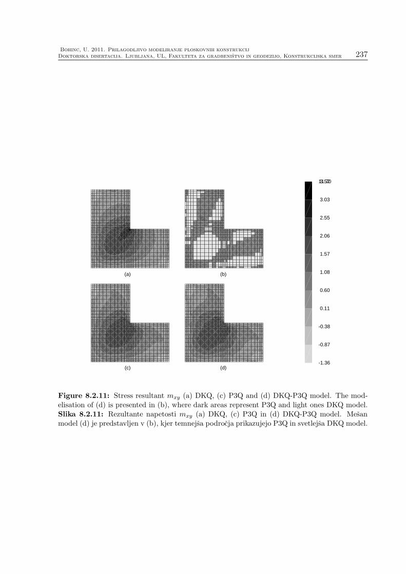
Bohinc, U. 2011. Prilagodljivo modeliranje ploskovnih konstrukcij
Doktorska disertacija. Ljubljana, UL, Fakulteta za gradbenistvo in geodezijo, Konstrukcijska smer 237
3.52
3.03
2.55
2.06
1.57
1.08
0.60
0.11
-0.38
-0.87
-1.36(d)(c)
(b)
11.70
(a)
Figure 8.2.11: Stress resultant mxy (a) DKQ, (c) P3Q and (d) DKQ-P3Q model. The mod-elisation of (d) is presented in (b), where dark areas represent P3Q and light ones DKQ model.Slika 8.2.11: Rezultante napetosti mxy (a) DKQ, (c) P3Q in (d) DKQ-P3Q model. Mesanmodel (d) je predstavljen v (b), kjer temnejsa podrocja prikazujejo P3Q in svetlejsa DKQ model.

238Bohinc, U. 2011. Adaptive modeling of plate structures
Doctoral thesis. Cachan, ENS Cachan, LMT
15.59
12.96
10.34
7.71
5.08
2.45
-0.18
-2.80
-5.43
-8.06
-10.69(d)(c)
(b)
11.70
(a)
Figure 8.2.12: Stress resultant qx (a) DKQ, (c) P3Q and (d) DKQ-P3Q model. The modeli-sation of (d) is presented in (b), where dark areas represent P3Q and light ones DKQ model.Slika 8.2.12: Rezultante napetosti qx (a) DKQ, (c) P3Q in (d) DKQ-P3Q model. Mesan model(d) je predstavljen v (b), kjer temnejsa podrocja prikazujejo P3Q in svetlejsa DKQ model.
70.00
60.00
50.00
40.00
30.00
20.00
10.00
[%]
100.00
80.00
0.00
90.00
Figure 8.2.13: Model error indicator for SKEW problemSlika 8.2.13: Ocena modelske napake za primer SKEW
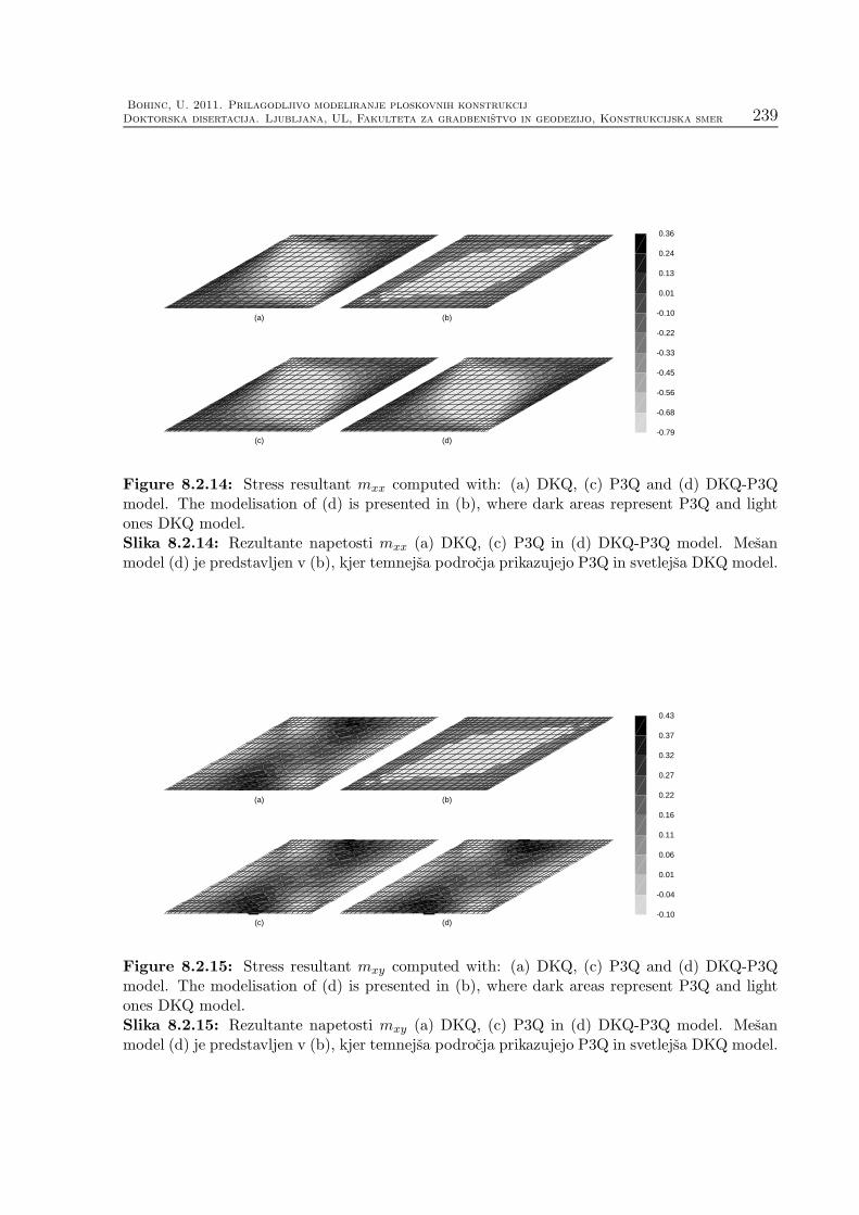
Bohinc, U. 2011. Prilagodljivo modeliranje ploskovnih konstrukcij
Doktorska disertacija. Ljubljana, UL, Fakulteta za gradbenistvo in geodezijo, Konstrukcijska smer 239
0.36
0.24
0.01
-0.10
-0.22
-0.33
-0.45
-0.56
-0.68
-0.79
(a) (b)
(d)(c)
0.13
Figure 8.2.14: Stress resultant mxx computed with: (a) DKQ, (c) P3Q and (d) DKQ-P3Qmodel. The modelisation of (d) is presented in (b), where dark areas represent P3Q and lightones DKQ model.Slika 8.2.14: Rezultante napetosti mxx (a) DKQ, (c) P3Q in (d) DKQ-P3Q model. Mesanmodel (d) je predstavljen v (b), kjer temnejsa podrocja prikazujejo P3Q in svetlejsa DKQ model.
0.32
0.27
0.22
0.16
0.11
-0.10
0.06
0.01
-0.04
0.43
0.37
(a) (b)
(d)(c)
Figure 8.2.15: Stress resultant mxy computed with: (a) DKQ, (c) P3Q and (d) DKQ-P3Qmodel. The modelisation of (d) is presented in (b), where dark areas represent P3Q and lightones DKQ model.Slika 8.2.15: Rezultante napetosti mxy (a) DKQ, (c) P3Q in (d) DKQ-P3Q model. Mesanmodel (d) je predstavljen v (b), kjer temnejsa podrocja prikazujejo P3Q in svetlejsa DKQ model.
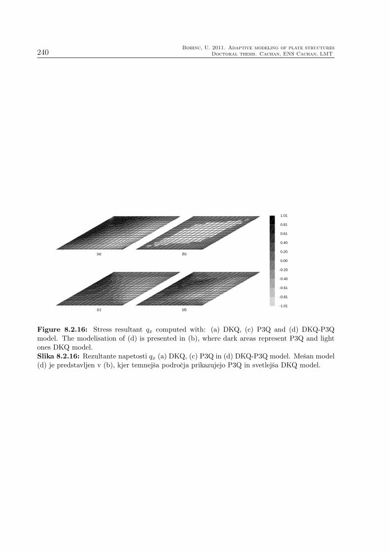
240Bohinc, U. 2011. Adaptive modeling of plate structures
Doctoral thesis. Cachan, ENS Cachan, LMT
-1.01
1.01
0.81
0.61
0.40
0.20
0.00
-0.20
-0.40
-0.61
-0.81
(a) (b)
(d)(c)
Figure 8.2.16: Stress resultant qx computed with: (a) DKQ, (c) P3Q and (d) DKQ-P3Qmodel. The modelisation of (d) is presented in (b), where dark areas represent P3Q and lightones DKQ model.Slika 8.2.16: Rezultante napetosti qx (a) DKQ, (c) P3Q in (d) DKQ-P3Q model. Mesan model(d) je predstavljen v (b), kjer temnejsa podrocja prikazujejo P3Q in svetlejsa DKQ model.

Bohinc, U. 2011. Prilagodljivo modeliranje ploskovnih konstrukcij
Doktorska disertacija. Ljubljana, UL, Fakulteta za gradbenistvo in geodezijo, Konstrukcijska smer 241
8.3 Chapter summary and conclusions
We have presented a detailed development for plate model adaptivity procedure capable of
selecting automatically the best suitable plate finite element between the two plate models,
the first for thin Kirchhoff plate and the second for thick Reissner/Mindlin plate. The
model adaptivity computation is carried out on the element basis, and it starts with the
finite element mesh which is first passed through the standard mesh adaptivity procedure
in order to achieve the acceptable discretization errors throughout the mesh. We addressed
in detail the particular case of two low-order plate finite element models, represented
with discrete Kirchhoff quadrilateral (DKQ) and Reissner/Mindlin quadrilateral (P3Q);
but the same procedure would carry over to higher-order plate models that capture more
accurately local 3D effects.
It is the key advantage of the presented approach to plate model adaptivity to re-
main uncoupled with respect to the mesh adaptivity procedure employed to reduce the
discretization error, and thus can be combined with any already available mesh adap-
tivity procedure to ensure the optimal overall accuracy. This advantage stems from the
proposed special choice of the finite element interpolations for both P3Q and DKQ plate
elements, which results with the same quality of the discrete approximation for bending
moments.
Numerical examples illustrate clearly that the proposed procedure is capable of cap-
turing any significant contribution of shear deformations. The case in point concerns the
shear layers which typically occur for different kinds of boundary conditions.

242Bohinc, U. 2011. Adaptive modeling of plate structures
Doctoral thesis. Cachan, ENS Cachan, LMT

Bohinc, U. 2011. Prilagodljivo modeliranje ploskovnih konstrukcij
Doktorska disertacija. Ljubljana, UL, Fakulteta za gradbenistvo in geodezijo, Konstrukcijska smer 243
Chapter 9
Conclusions
The thesis is related to adaptive modeling of plates. Although the finite element modeling
of plates reached a mature phase, the reflection shows that the fundamental questions of
accuracy and reliability are still open and need to be properly addressed.
Before addressing the subject of adaptive modeling, two basic and one new plate
theories are first studied in detail in chapters 2-4. The phenomena intrinsic to the plate
modeling are identified and studied. The corresponding finite element formulation are
presented in a way which respects the natural hierarchy present in modeling of plate
structures. A Discrete Kirchhoff element, which is one of the most popular elements for
the analysis of thin plates, was reformulated using an alternative notation, which enables
general treatment of triangular and quadrilateral formulations. Moreover, the presented
formulation for the DK elements enables the hierarchic (in a model sense) construction
of the finite elements based on Reissner/Mindlin theory. The elements, denoted P3, are
constructed as the hierarchic extension of the DK elements. The elements built on the
higher-order theory including through-the-thickness stretch are further built on the basis
of P3 elements. This type of hierarchic construction helps to maintain the physical insight
despite the increasing complexity of the finite element formulation.
Additionally, conforming triangular plate element for thin plates is presented as well as
incompatible modes finite elements for Reissner/Mindlin plates. All presented plate ele-
ments were implemented in finite element analysis computer codes and tested. Systematic
comparison of the element performance through a series of numerical tests is performed.
This comparison in itself presents a valuable contribution to the subject of finite element
modeling of plate structures.
The research on discretization error estimates for finite element computation is active
and today many results are available regarding the general treatment of the subject. In

244Bohinc, U. 2011. Adaptive modeling of plate structures
Doctoral thesis. Cachan, ENS Cachan, LMT
this work some of the results are applied to the case of finite element modeling of plate
structures. When using dimensionally reduced models, specific numeric issues (locking)
appear. Phenomena intrinsic to plates require deeper understanding of the subject of
error estimates. The application of the existing error estimation methods to the plate
elements is thus not straightforward. A large part of the research work presented in thesis
is related to the successful implementation of the equilibrated residual method (EqR) for
the DK plate element. The implementation of the EqR method is challenging, among
other things, mostly from the technical point of view. The computation process involves
several steps: (i) computation of equilibrated boundary traction from the original finite
element solution, (ii) setup of local element problems loaded with boundary tractions,
(iii) solution of local problems with enhanced interpolation space and (iv) computation
of the discretization error estimate from the local solution.
Several variations of the EqR method were implemented: the local computations were
performed with various enhanced interpolations. Enhancing the interpolation space with
the subdivision of existing element proved to be an efficient alternative to the more in-
volved computation using the conforming element. This type of study has not been
attempted before and thus presents a new contribution to the subject of discretization
error estimates for plates. The comparison of the performance of EqR method and com-
monly accepted superconvergent patch recovery (SPR) method is presented by several
numerical examples. Additionally, an adaptive construction of a mesh based on the esti-
mation of discretization error is illustrated on a numerical example. Both methods have
its own advantages: the EqR method provides noticeable higher local accuracy of the
error estimates, while the SPR is significantly easier to implement. The EqR method
proved to be a reasonable alternative to the SPR method.
Model error concept is discussed in chapters 7-8. Following the general treatment of
the principles of model error estimation, a method of model error estimation based on
the EqR method is proposed. Specific issues related to the construction of local problems
for the plate elements are addressed in chapter 8. Several numerical tests illustrate the
performance of the proposed method. The proposed method proved to be capable of
detecting the areas with increased model error.
The work presented in this thesis showed another important conclusion: the hierarchy
of the plate finite element models involved in the model error estimation procedure is the
key to the successful model error estimation. It is only the use of hierarchic (in the model
sense) family of plate elements which enabled the successful implementation of model

Bohinc, U. 2011. Prilagodljivo modeliranje ploskovnih konstrukcij
Doktorska disertacija. Ljubljana, UL, Fakulteta za gradbenistvo in geodezijo, Konstrukcijska smer 245
error estimates based on EqR.
An illustration of iterative adaptive construction of the optimal finite element model
based on the computation of the model error indicator is presented. The example shows,
that the proposed model error indicator is capable of driving the adaptive procedure.
Another important conclusion that was found out during the study of model error
estimates is the fact that the maxim: ‘build the model from coarse to fine’ has its limits.
It was shown namely that it is impossible to detect the boundary layer phenomena using
the results of the coarse model only. It is therefore not realistic to expect from the
proposed model error estimation method to detect phenomena which intrinsically depend
on the complexity of the model itself. The coarse model just does not carry enough
information to be able to detect a possible higher order phenomena. In order to capture
all the important phenomena in a certain plate model using adaptive modeling, the initial
model should not be too coarse.
To summarize: the main goal of the thesis was to implement and test the key element of
the concept of adaptive modeling of plates: error estimates. Some of the most promising
methods were explored and tested. The results presented in this thesis show that the
studied error estimates are suitable for the purpose of adaptive modeling. This work
thus indicates that it would be possible to construct a fully automated procedure for the
determination of the optimal finite element model of a given plate problem.

246Bohinc, U. 2011. Adaptive modeling of plate structures
Doctoral thesis. Cachan, ENS Cachan, LMT

Bohinc, U. 2011. Prilagodljivo modeliranje ploskovnih konstrukcij
Doktorska disertacija. Ljubljana, UL, Fakulteta za gradbenistvo in geodezijo, Konstrukcijska smer 247
Chapter 10
Razsirjeni povzetek
10.1 Motivacija
Razumevanje obnasanja konstrukcij pod razlicnimi obremenitvami ima ze od nekdaj ve-
lik pomen za clovekov razvoj. Zgodovinsko gledano, je vecji del znanja o konstrukcijah
clovek pridobil s preskusanjem. Vendar pa je zaradi narascajoce kompleksnosti grajenih
objektov kmalu postalo jasno, da ni mogoce in tudi ne ekonomicno, da bi s preskusanjem
dolocili odpornost konstrukcije v vseh moznih obteznih primerih. Spoznanje je vodilo v
razvoj modelov fizikalnih procesov, s katerimi je mogoce racunsko napovedati obnasanje
konstrukcij. Ker so modeli zgrajeni na podlagi eksperimentalnih rezultatov, njihova
natancnost ne more preseci natancnosti, s katero izvajamo preskus. Natancnost mod-
elske napovedi je hkrati omejena s koncno racunsko mocjo, ki neposredno vpliva na raven
podrobnosti, ki jo je moc opisati z danim racunskim modelom.
V zgodnjih letih razvoja je bil analiticni nacin resevanja racunskih modelov edini
dosegljiv nacin. Z njim je bilo mogoce obravnavati le probleme s preprosto geometrijo
in snovnimi zakoni. Metode za priblizno racunsko resevanje modelov so bile sicer kmalu
razvite, vendar so bile bistveno omejene z racunsko mocjo resevalca (v tem casu je bil to
vecinoma clovek). Svoj silovit vzpon so dozivele sele s pojavom sodobnih racunalnikov.
Sorazmerno kmalu po zacetku uporabe je bilo mogoce z njimi resevati tudi kompleksne
inzenirske probleme. Dandanes so racunski modeli postali sestavni del projektiranja. Na
podlagi izracunov se sprejemajo kriticne odlocitve in zakljucki. Iz tega razloga je definicija
zanesljivosti in natancnosti modelskih napovedi posebnega pomena.
Razumevanje izbranega fizikalnega pojava je popolno sele, ko lahko izracunamo oziroma
napovemo izid preskusa, s katerim ga preverjamo. Model dolocenega fizikalnega pojava
je sprejet, ko se njegove napovedi ujemajo z izidi nadzorovanih preskusov. Ker inzenirski
pristop k modeliranju temelji na paradigmi: ”tako preprosto, kot je le mogoce in le

248Bohinc, U. 2011. Adaptive modeling of plate structures
Doctoral thesis. Cachan, ENS Cachan, LMT
tako zapleteno, kot je potrebno”, je zahtevana raven kompleksnosti modela izbranega
fizikalnega pojava dolocena s zahtevano natancnostjo napovedi.
Razliko med izmerjeno fizikalno stvarnostjo in modelskimi napovedmi lahko pripisemo
enemu od dveh razlogov: (i) bodisi je model grajen na napacnih predpostavkah in/ali
(ii) je resitev modela je le priblizna. Napaki modelske napovedi, katere vzrok so napacne
predpostavke, obicajno pravimo modelska napaka. Priblizno resevanje modela je vzrok
diskretizacijski napaki.
10.1.1 Verifikacija in validacija
Skupna napaka napovedi je tako vedno vsota modelske in diskretizacijske napake. Ce
je modelska napaka posledica priblizkov, storjenih pri zapisu sistema enacb, ki opisu-
jejo izbran fizikalni pojav, je diskretizacijska napaka tista, ki nastane zaradi pribliznega
resevanja teh istih enacb. Za studij natancnosti izbranega modela je bil razvit koncept
verifikacije in validacije: verifikacija je primerjava priblizne resitve (diskretizirane ra-
zlicice) modela s tocno resitvijo, validacija pa je primerjava modelskih napovedi z izidom
preskusov.
Model je matematicna idealizacija fizikalnega modela, ki je zgrajen na dolocenih pred-
postavkah in poenostavitvah. Pri definiciji modela je tako vedno prisotna dolocena stopnja
abstrakcije, ki obicajno vsebuje koncept zveznosti. Ta predpostavlja, da je resitev znana v
vsaki tocki obmocja. Tak model racunsko ni resljiv, saj je stevilo tock v sistemu (in s tem
neznank) neskoncno. Da bi dobili racunsko resljiv sistem, model diskretiziramo s koncnim
stevilom neznank. Siroko uveljavljena metoda diskretizacije zveznih matematicnih mode-
lov, ki jih opisujejo parcialne diferencialne enacbe, je metoda koncnih elementov (MKE).
Diskretizacija sistema prinese dodatno napako, ki ji pravimo diskretizacijska napaka.
Metoda koncnih elementov je bila zasnovana s strani inzenirjev in matematikov pred-
vsem za resevanje problemov s podrocja linearne elasticnosti. Tudi dandanes metoda
koncnih elementov ostaja zlasti na podrocju linearne mehanike konstrukcij. V isto po-
drocje spada tudi zarisce tega dela: analiza upogiba ploskovnih konstrukcij z metodo
koncnih elementov.
10.1.2 Prilagodljivo modeliranje - optimalni model
Da bi nasli optimalni model za analizo izbrane ploskovne konstrukcije, moramo najprej
dolociti primerne kriterije. Ce je edini kriterij natancnost modelske napovedi, je na-
jprimernejsi model polni trirazsezni model. Vendar pa zaradi velike racunske zahtevnosti

Bohinc, U. 2011. Prilagodljivo modeliranje ploskovnih konstrukcij
Doktorska disertacija. Ljubljana, UL, Fakulteta za gradbenistvo in geodezijo, Konstrukcijska smer 249
taka izbira ni posebej racionalna. Optimalnost modela zato definiramo v inzenirskem
smislu: optimalni model je najpreprostejsi model, ki se dosega zahtevano natancnost.
Plosce so osnovni konstrukcijski elementi in za opis njihovega obnasanja je bilo razvitih
vec modelov. Ker je tretja razseznost plosc znatno manjsa kot preostali dve, uporabljamo
za modele plosc nacelo dimenzijske redukcije. Racunska prednost uporabe dvorazseznih
modelov pred trirazseznimi je ocitna. Ceprav modeli plosc asimptoticno konvergirajo k
trirazseznemu modelu, niso vsi zgrajeni na nacelih asimptoticne analize. Vec uspesnih
modelov plosc je bilo razvitih na podlagi a-priori predpostavk, ki so izsle iz globokega
inzenirskega uvida. Kljub temu je mogoce, glede na konvergenco k polnemu trirazseznemu
modelu, vzpostaviti hierarhijo med modeli. Mogoce je oblikovati druzino hierarhicno
urejenih modelov plosc - vrsto modelov, katerih resitve konvergirajo k tocni trirazsezni
resitvi problema upogiba plosc. Konvergenca k tocni trirazsezni resitvi se kaze, med
drugim, v zmoznosti opisa posebnih robnih pojavov, ki so znacilni za trirazsezne resitev.
Predpostavke, na katerih slonijo modeli plosc, so obicajno povezani s kinematiko de-
formacije. Ta je mocno odvisna od robnih pogojev, koncentrirane obtezbe in skokovitih
sprememb v debelini ali snovnih lastnostih. Ker je kinematika krajevno odvisna, enako
velja tudi za veljavnost modelskih predpostavk. Model je optimalen le v obmocju, kjer
veljajo njegove predpostavke. Iz tega izhaja, da je optimalni model odvisen od kraja, ven-
dar pa enotnega modela, ki bi bil optimalen po celotnem obmocju, obicajno ni. Obmocje
zato razdelimo v podrocja. Vsakega od podrocij modeliramo s svojim optimalnim mod-
elom. Cilj prilagodljivega modeliranja je prepoznati ta podrocja in za vsakega od njih
dolociti svoj optimalni model.
Krajevno odvisen optimalni model ploskovne konstrukcije lahko zgradimo iterativno, v
vec korakih. Inzenirski pristop h gradnji optimalnega modela sloni na nacelu: od grobega
proti bolj podrobnemu. Prvo analizo problema izvedemo z najbolj grobim modelom po
celotnem obmocju. Z obdelavo resitve dobimo oceno modelske napake. Glede na pred-
pisano natancnost prepoznamo obmocja, kjer je napaka vecja od predpisane in bi morali
uporabiti boljsi, bolj rafiniran model. Zgradimo nov mesan model, in izracunamo novo
resitev. Spet ocenimo modelsko napako in dolocimo podrocja, kjer je potrebno uporabiti
boljsi model. Postopek ponavljamo tako dolgo, dokler ne dosezemo zahtevane natancnosti
po celotnem obmocju. Kljucni element tega postopka je ucinkovita in tocna ocena mod-
elske napake.
Ko izberemo krajevno odvisen optimalni model, ga diskretiziramo, da dobimo racunsko
resljiv sistem enacb. Diskretizacija po metodi koncnih elementov razdeli racunsko obmocje
250Bohinc, U. 2011. Adaptive modeling of plate structures
Doctoral thesis. Cachan, ENS Cachan, LMT
na koncne elemente. Na vsakem od elementov zgradimo priblizek resitve, ki je odvisen od
koncnega stevila prostostnih stopenj. Kakovost priblizka je odvisna od velikosti elementa
in razgibanosti resitve - bolj, ko je resitev spremenljiva, manjse elemente potrebujemo, da
jo zadovoljivo opisemo. Pri optimalni diskretizaciji je diskretizacijska napaka enakomerno
razdeljena po celem obmocju in je priblizno enaka za vse elemente, ne glede na velikost.
Diskretizacijsko napako uravnavamo s spreminjanjem velikosti elementov. Gradnja op-
timalne diskretizacije (ali mreze) je obicajno iterativna. Najprej izracunamo resitev na
sorazmerno grobi mrezi in izracunamo oceno diskretizacijske napake. Ker je odvisnost
diskretizacijske napake od velikosti elementa poznana a-priori, lahko, ce je dolocena za-
htevana natancnost resitve, na podlagi ocene diskretizacijske napake ocenimo velikost
elementa. Na tak nacin dobimo oceno porazdelitve velikosti elementov po obmocju in
z upostevanjem te ocene zgradimo novo mrezo. To ponavljamo tako dolgo dokler ne
dosezemo predpisane natancnosti in zagotovimo enakomerno porazdelitev diskretizacijske
napake po elementih.
Optimalni model, v smislu modelske in diskretizacijske napake, je prilagojen izbranemu
problemu. Glavna prednost prilagodljivega modeliranja ni toliko v obcutnem povecanju
racunske ucinkovitosti, kolikor je v nadzoru nad natancnostjo modelskih napovedi. Samod-
ejni postopek za izbiro optimalnega modela preprecuje neizkusenemu uporabniku ne-
upravicene poenostavitve, ki lahko zabrisejo morebitne koncentracije napetosti. Po drugi
strani pa je, zaradi vedno vecje racunske moci, skusnjava po izbiri prevec podrobnih mod-
elov vedno vecja. Ceprav ti zajamejo vse podrobnosti, jih je bistveno tezje interpretirati
in mnogokrat prav podrobnosti zasencijo bistvene znacilnosti resitve.
10.1.3 Napaka diskretizacije, modelska napaka
Prilagodljivo modeliranje je iterativni proces, ki temelji na ocenah modelske in diskretizaci-
jske napake. Pri obravnavi napake je potrebno jasno lociti med oceno in cenilko napake.
Cenilke obicajno podajajo zgornjo in spodnjo mejo napake. Ker je mogoce dokazati, da
napaka lezi znotraj napovedanih meja, so cenilke precej konzervativne. Slaba stran jam-
stva, ki ga dajejo cenilke se odraza v bistveno precenjeni napaki. Po drugi strani ocene
napake ne dajejo nobenih jamstev, temvec omogocajo precej natancno indikacijo napake.
Namen racuna napake doloca izbiro med cenilkami in ocenami. V primerih, kjer je glavni
cilj racuna napake vodenje postopka prilagodljivega modeliranja, se uporabljajo ocene
napake.
Za uspesno gradnjo optimalnega modela je kljucen ucinkovit izracun zanesljive ocene

Bohinc, U. 2011. Prilagodljivo modeliranje ploskovnih konstrukcij
Doktorska disertacija. Ljubljana, UL, Fakulteta za gradbenistvo in geodezijo, Konstrukcijska smer 251
napake: tako diskretizacijske, kot tudi modelske. Ceprav slednja lahko bistveno preseze
diskretizacijsko napako, jo je precej tezje oceniti. To se odraza v majhnem stevilu ob-
stojecih metod za izracun ocene modelske napake. Ker obstojece metode oceno modelske
napake obravnavajo na precej splosni ravni, se v tem delu osredotocamo na izracun ocene
modelske napake za primer modeliranja plosc. Razvoj postopka za oceno modelske na-
pake za primer analize plosc s koncnimi elementi predstavlja enega glavnih dosezkov tega
dela.
Ucinkovit postopek za izracun ocene modelske napake izhaja iz naslednje zamisli: mod-
elska napaka meri razliko med resitvijo z obstojecim modelom in resitvijo z referencnim
modelom - polnim trirazseznim modelom. Globalni racun tocne resitve z referencnim
modelom - samo zato, da bi resitev primerjali z obstojeco resitvijo - je seveda predrag.
Zato poskusimo izracunati resitev z referencnim modelom na manjsih obmocjih - najbolje
kar na koncnih elementih. Pri tem moramo poskrbeti, da lokalni izracuni cim bolj verno
nadomestijo globalni izracun. Pri tem si predstavljamo, da obmocja, na katerih izvajamo
lokalni izracun, izlocimo iz kontinuuma in delovanje okolice predstavimo z robno obtezbo.
Zato so robni pogoji za lokalne izracune Neumannovega tipa.
Osrednje vprasanje ocene modelske napake tako postane: ”Kako oceniti robne pogoje
za lokalne izracune?”, ce bi poznali tocno resitev, bi robne pogoje lahko dolocili iz napetosti
s pomocjo Cauchijevega principa. Ker pa tocne resitve seveda ne poznamo, se pri oceni
napetosti opremo na edino dosegljivo informacijo: trenutno resitev s koncnimi elementi.
Ker resitev s koncnimi elementi predstavlja priblizek tocne resitve, lahko iz nje ocenimo
napetosti, ki so podlaga za izracun robnih pogojev. Razvoj metod za izracun najboljse
ocene robnih pogojev za lokalne izracune, je tako kljucen del izracuna ocene modelske
napake.
Uporaba te preproste zamisli na primeru modeliranja plosc ni zelo preprosta, saj je
potrebno smiselno upostevati posebne pojave, ki so znacilni le za modeliranje plosc. Za-
htevnost implementacije povecuje tudi dejstvo, da je vecina koncnih elementov za plosce
nekompatibilnih.
10.2 Cilji
Glavni cilji naloge se nanasajo na koncept prilagodljivega modeliranja ploskovnih kon-
strukcij. Prvi cilj naloge je zato razvoj hierarhicne druzine (v modelskem smislu) dobro
delujocih trikotnih in stirikotnih koncnih elementov za plosce.

252Bohinc, U. 2011. Adaptive modeling of plate structures
Doctoral thesis. Cachan, ENS Cachan, LMT
Ker je koncept prilagodljivega modeliranja kljucno odvisen od zanesljivih ocen napak,
se drugi cilj naloge nanasa predvsem na oceno napake diskretizacije: cilji so izpeljava, im-
plementacija ter testiranje nekaj najbolj uveljavljenih a-posteriori metod za oceno napake.
Pri tem se osredotocamo na dve najbolj prepoznavni metodi: SPR ( supercovergent patch
recovery) in EqR (method of equilibrated residuals). Metodi sta implementirani za primer
DK in RM ploscnih elementov, ki so najbolj pogosto uporabljeni za analizo ploskovnih
konstrukcij z metodo koncnih elementov.
Trenutno je za oceno napake diskretizacije razvitih bistveno vec metod kot za oceno
modelske napake. V tem delu se za oceno modelske napake zanasamo na metodo, ki
temelji na EqR metodi. Tretji cilj te naloge je pojasniti in izpeljati uporabo EqR metode
za oceno modelske napake.
Zadnji cilj naloge je izpeljati proceduro za prilagodljivo modeliranje plosc. Ta naj
bi sledila naslednjim korakom: izracunaj zacetno resitev izbranega problema s koncnimi
elementi, oceni modelsko napako in napako diskretizacije, na podlagi ocene napak kon-
struiraj boljsi model (s koncnimi elementi) problema. Prilagodljivo modeliranje naj bi
sledilo konceptu gradnje od spodaj navzgor: od sorazmerno grobega modela in mreze
do modela, ki je sposoben opisati vse pomembne pojave in pri tem nadzorovati skupno
napako, kakor tudi njeno porazdelitev po obmocju.
10.3 Zgradba naloge
Nalogo sestavlja devet poglavij. V prvem poglavju sta podana pregled in trenutno stanje
podrocja.
V poglavjih 2 do 4 je predstavljen pregled teorije plosc. Teorije so razvrscene od bolj
preprostih do ”kvazi” tridimenzionalnih. Teoreticna obravnava plosc razkriva nekatere
pojave, ki so tipicni le zanje: singularnosti ter robna obmocja. Opis teorij, ki jih je
mogoce hierarhicno urediti, je dopolnjen z nekaj mogocimi diskretizacijami: koncnimi
elementi. Predstavljenih je nekaj najpomembnejsih in uveljavljenih koncnih elementov.
Poglavja so zakljucena z obravnavo nekaj testnih primerov, ki ilustrirajo razlicne vidike
modeliranja plosc s koncnimi elementi.
Poglavje 5 se zacne s pregledom najpomembnejsih metod za oceno napake diskretizacije.
Splosnemu opisu sledi podrobnejsa obravnava metod SPR in EqR. Implementaciji EqR
metode je namenjena posebna pozornost v poglavju 6. Implementacija je nekoliko za-
htevnejsa za primer ne-konformnih koncnih elementov in v literaturi se ni bila podrobneje

Bohinc, U. 2011. Prilagodljivo modeliranje ploskovnih konstrukcij
Doktorska disertacija. Ljubljana, UL, Fakulteta za gradbenistvo in geodezijo, Konstrukcijska smer 253
opisana. Vec numericnih primerov prikazuje razlike med posameznimi metodami ocene
napake diskretizacije.
Poglavji 7 in 8 se ukvarjata z vprasanjem modelske napake. Splosni obravnavi mod-
elske napake sledi opis nacina ocene modelske napake, ki sloni na metodi uravnotezenih
residualov. Posebna pozornost je namenjena implementaciji metode za primer koncnih
elementov za plosce, ki so predstavljeni v poglavjih 2-4. Ucinkovitost metode je prikazana
z vec izbranimi numericnimi primeri.
Zakljucki in povzetek so podani v poglavju 9.
10.4 Plosce
Ploskovne konstrukcije so konstrukcije, katerih debelina je bistveno manjsa od razpona.
Povsem jih dolocata v ravnini lezeca nevtralna ploskev in njihova debelina. V nadaljevanju
se bomo osredotocili na studij odziva ploskovnih konstrukcij na delovanje precne obtezbe.
Krajse ploskovne konstrukcije imenujemo kar plosce.
Obnasanje plosc pri delovanju precne obtezbe prvenstveno doloca razmerje med razponom
in debelino plosce. Med tanke plosce stejemo plosce, pri katerih je to razmerje okvirno
med 100 in 20. Zanje je znacilno, da je mogoce precne strizne deformacije zanemariti.
Pri ploscah z razmerjem med 20 in 5, ki jih imenujemo srednje debele, je strizna defor-
macija koncna in jo moramo upostevati pri izracunu. Pri debelih ploscah, pri katerih je
razmerje med razponom in debelino manjse od 5, moramo upostevati tudi deformacije
vzdolz debeline plosce. Deformacijsko polje takih plosc je tako ze zelo blizu polnemu
tri-dimenzionalnemu deformacijskemu stanju.
10.4.1 Tanke plosce
Model
V drugem poglavju obravnavamo upogib linearno elasticnih tankih plosc, pri cemer se
opremo na glavno predpostavko t.i. Kirchhoffovega modela: ravna vlakna, ki pred de-
formacijo lezijo pravokotno na nevtralno ravnino, ostanejo ravna in pravokotna nanjo
tudi po deformaciji. Nevtralno ploskev sestavljajo tocke, ki se premaknejo le v smeri
z. Pomik tocke P (x, y, 0) na nevtralni ploskvi je dolocen s precnim pomikom w(x, y).
Pomik poljubne tocke P (x, y, z), ki lezi na razdalji z od nevtralne ravnine, je dolocen z
naslednjim izrazom (glej tudi Sliko 2.2.1):
ux = +zθy ; uy = −zθx; uz = w

254Bohinc, U. 2011. Adaptive modeling of plate structures
Doctoral thesis. Cachan, ENS Cachan, LMT
Pri tem je s θ = [θx, θy]T oznacena rotacija vlakna, na katerem lezi izbrana tocka. Ker je
vlakno pravokotno na nevtralno ravnino, je njegova rotacija dolocena z nagibom nevtralne
ploskve (2.2.1):
θx = +∂w
∂y; θy = −∂w
∂x
Deformacijsko polje, ki ustreza Kirchhoffovi predpostavki, je naslednje oblike (2.2.2):
εxx = −∂2w
∂x2; εyy = −∂
2w
∂y2; εxy = − ∂2w
∂x∂y
εzz = 0; εxz = 0; εyz = 0
Za bolj kompaktni zapis uvedemo vektor ukrivljenosti (2.2.8)
κ = [∂2w
∂x2,∂2w
∂y2, 2
∂2w
∂x∂y]T
in zapisemo (2.2.5)
εxx = −zκxx; εyy = −zκyy ; γxy = 2εxy = −zκxy
Predpostavimo ravninsko napetostno stanje (σzz = 0), iz cesar dobimo (2.2.10). Z uvedbo
rezultant napetosti (2.2.11) v obliki vektorja m = [mxx, myy, mxy]T dobimo naslednjo
relacijo (2.2.12)
m = CBκ
kjer je konstitutivna matrika oblike (2.2.13)
CB = D
1 ν 0ν 1 00 0 1
2(1− ν)
s konstanto D = 112Et3/(1− ν2), ki predstavlja izotropno togost plosce.
Ravnotezje diferencialnega elementa (glej Sliko 2.2.2) je doloceno z enacbama (2.2.16)
in (2.2.17). Z eliminacijo strizne sile q zapisemo ravnotezje v obliki (2.2.19) :
∂2mxx
∂x2+ 2
∂2mxy
∂x∂y+∂2myy
∂y2= f
kjer je f precna obtezba plosce.
Zgornje enacbe zdruzimo v znano biharmonicno enacbo(2.2.26)
∂4w
∂x4+ 2
∂4w
∂x2∂y2+∂4w
∂x4= f/D

Bohinc, U. 2011. Prilagodljivo modeliranje ploskovnih konstrukcij
Doktorska disertacija. Ljubljana, UL, Fakulteta za gradbenistvo in geodezijo, Konstrukcijska smer 255
Diferencialna enacba skupaj z robnimi pogoji predstavlja matematicno formulacijo up-
ogiba tankih plosc v mocni obliki.
Ker je diferencialna enacba cetrtega reda, sta na robu po dva robna pogoja, kar je v
navideznem nasprotju s tremi kolicinami, ki so konjugirane h komponentam pomika na
robu: (i) k precnemu pomiku w - precna strizna sila q, (ii) k zasuku v smeri roba θs -
rezultanta momenta v smeri roba ms in k pravokotnemu zasuku na rob θn - rezultanta
momenta pravokotno na rob mn (glej Sliko 2.2.4). Obravnava sibke formulacije problema
(2.2.43) pokaze, da je nasprotje le navidezno, ker zaradi Kirchhoffove predpostavke zasuk
pravokotno na rob θn = ∂w∂s
ni neodvisen, temvec enolicno dolocen s potekom pomika po
robu. Na robu tanke plosce sta zato dve neodvisni komponenti obtezbe: (i) efektivna
precna sila qef , ki je konjugirana k precnemu pomiku, ter (ii) moment vzdolz roba ms, ki
je konjugiran k zasuku, ki vrti vzdolz roba. Efektivna precna sila je definirana z izrazom
(2.2.44).
qef = q − ∂mn
∂s
Na prostem robu tako velja qef = 0 in ms = 0, kar pomeni, da sta na prostem robu lahko
razlicni od nic tako precna sila q 6= 0, kakor tudi rezultanta momenta mn 6= 0.
Posledica Kirchhoffove predpostavke, ki veze zasuk plosce s pomikom, je tudi pojav
t.i. ”koncentrirane” sile v nepodprtih vogalih plosce. Integracija per partes (po robu
od tocke A do tocke B) v (2.2.43), ki pripelje do efektivne strizne sile, povzroci dodatni
clen oblike [umn]BA . Po upostevanju zveznosti precnega pomika, dodatni clen skupaj
prispeva vsoto∑
I uI(mn,I |B −mn,I |A), kjer so z I oznacene tocke na robu. Cleni vsote
so razlicni od nic le v tistih tockah I vzdolz roba ΓN,AB, kjer velja nezveznost mn,I |B 6=mn,I |A. Pri tem smo uporabili oznako mn,I |A za vrednost mn v tocki I pri priblizevanju
s strani tocke A. Te cleni, ki k virtualnemu delu zunanjih sil prispevajo∑
I uIFC,I , kjer
FC,I = [mn,I ]BA , razumemo kot koncentrirano silo v tocki I. Ce se omejimo na reakcije, je
koncentrirana sila razlicna od nic le v tockah prosto podprtega roba, kjer se smer robu
nezvezno spremeni (kjer ima plosca vogal) (2.2.47). V primeru, ko je vogal togo vpet ali
prost, je koncentrirana sila FC,I enaka 0.
Princip virtualnega dela za tanke plosce se glasi: v ravnovesju je virtualno delo zu-
nanjih sil δΠext enako virtualnemu delu notranjih sil δΠint: δΠint = δΠext za poljuben
virtualni pomik δw, ki ustreza Kirhhoffovi predpostavki ter robnim pogojem (Tabela
2.1), pri cemer je
δΠint =
∫
Ω
δκTm dΩ; δΠext =
∫
Ω
δw f dΩ +
∫
Γ
(qefδw −msδ∂w
δn) ds

256Bohinc, U. 2011. Adaptive modeling of plate structures
Doctoral thesis. Cachan, ENS Cachan, LMT
Virtualna pomika na robu plosce δw in δ∂wδn
sta neodvisna. K njima sta konjugirani obtezbi
qef in ms. Z uporabo konstitutivne relacije m = CBκ = CBLκ lahko pokazemo, da je
princip virtualnega dela ekvivalenten biharmonicni enacbi.
Zanimiva posledica Kirchhoffove predpostavke je obstoj ”singularnosti”, ki nastane v
dolocenih primerih krivega roba, ko je ta interpoliran z lomljenim robom. Zaradi Kirchhof-
fove predpostavke je na vogalu takega roba, normalna komponenta rotacije θn definirana
dvakrat - v dveh smereh, zaradi cesar je vogal efektivno vpet. To lahko povzroci sin-
gularnost v rezultantah napetosti. Vodilni clen, ki doloca, kako izrazita je singularnost,
opisemo z izrazom rλ−2 za rezultante momentov ter rλ−3 za strizne sile. Eksponent λ je
odvisen od robnih pogojev ter obratno sorazmeren kotu α, ki ga oklepa vogal. Singu-
larnost za rezultante momentov nastopi, kadar je λ < 2 (oziroma λ < 3 za strizne sile).
Kriticni koti, kjer nastopi singularnost, so podani v Tabeli 2.2. Za primer dvakrat prosto
podprtega vogala tako preberemo, da singularnost striznih sil nastopi, ko je α > 60 in
za rezultante momentov, ko je α > 90.
Koncni elementi
Iz principa virtualnega dela za tanke plosce vidimo, da v njem nastopajo najvec drugi
odvodi w. Interpolacija w mora biti zato najmanj zvezno odvedljiva C1, hkrati mora tudi
tocno opisati vse polinome do vkljucno drugega reda. Izkaze se, da je koncne elemente, ki
ustrezajo obema zahtevama, tezko konstruirati. Obicajno se za modeliranje odziva tankih
plosc uporabljajo koncni elementi, ki krsijo zahtevo po zvezni odvedljivosti, zaradi cesar
jim pravimo nekompatibilni v nasprotju s kompatibilnimi ali konformnimi elementi, ki tej
zahtevi zadostijo.
V nadaljevanju je najprej predstavljen trikotni konformni element imenovan ARGY
([Argyris et al., 1968]). Zaradi velikega stevila prostostnih stopenj, ki nimajo prave
fizikalne interpretacije, se element zelo redko uporablja za prakticne izracune. Nasprotje
so nekompatibilni elementi tipa DK [Dhatt, 1970], [Batoz et al., 1980], [Batoz, 1982], ki
uporabljajo interpolacijo pomika, ki ni zvezno odvedljiva. Ime DK (Diskretni Kirchhoff)
izhaja iz dejstva, da interpolacija zadosti Kirchhoffovi predpostavki le v diskretno mnogo
tockah. Konvergenca elementov tega tipa je zagotovljena, ker prestanejo t.i. ”patch test”.
Kljub omenjenim lastnostim, so elementi DK zelo priljubljeni, saj so v mnogo primerih
bolj ucinkoviti od konformnih elementov.

Bohinc, U. 2011. Prilagodljivo modeliranje ploskovnih konstrukcij
Doktorska disertacija. Ljubljana, UL, Fakulteta za gradbenistvo in geodezijo, Konstrukcijska smer 257
Konformni trikotni element (2.3.4)
Interpolacija za trikotni konformni element ARGY predstavlja popolni polinom petega
reda (z 21 parametri). To je najnizja stopnja, ki se zadosca pogoju zvezne odvedljivosti
pri prehodu cez rob elementa. Interpolacija je zapisana v naravnem trikotniskem koordi-
natnem sistemu (2.3.21) (ζ1, ζ2, ζ3):
wh = ωT p
kjer je p vektor vozliscnih parametrov in ω mnozica interpolacijskih funkcij, ki vsebuje
21 elementov :
ω = [ζ51 , ζ52 , ζ
53 ,
ζ1ζ42 , ζ2ζ
43 , ζ3ζ
41 , ζ2ζ
41 , ζ3ζ
42 , ζ1ζ
43 ,
ζ31ζ22 , ζ
32ζ
23 , ζ
33ζ
21 , ζ
32ζ
21 , ζ
33ζ
22 , ζ
31ζ
23 ,
ζ31ζ2ζ3, ζ1ζ32ζ3, ζ1ζ2ζ
33 , ζ
21ζ
22ζ3, ζ
21ζ2ζ
23 , ζ1ζ
22ζ
23 ]
T
Prostostne stopnje elementa se nanasajo na 3 vozlisca v ogliscih ter 3 vozlisca na sredini
stranic. Vsako oglisce ima 6 prostostnih stopenj: precni pomik, njegove prve odvode,
ter druge odvode glede na smeri x in y. Vozlisce v sredini stranice ima eno prostostno
stopnjo, ki se nanasa na odvod pomika v smeri normale stranice. Mnozica prostostnih
stopenj elementa w je tako (Slika 2.3.7):
w = [w1, w2, w3, w1,x, w1,y, w2,x, w2,y, w3,x, w3,y,
w1,xx, w1,xy, w1,yy, w2,xx, w2,xy, w2,yy, w3,xx, w3,xy, w3,yy,
w,n12, w,n23, w,n31 ]T
Da bi dolocili povezavo med prostostnimi stopnjami w ter parametri p, moramo izracunati
odvode v vozliscih. Kot vmesni korak vpeljemo prostostne stopnje wρ, ki se nanasajo na
trikotniske koordinate:
wρ = [ w1, w2, w3, w1,12, w1,31, w2,23, w2,12, w3,31, w3,23,
w1,122 , w1,312 , w1,232 , w2,122, w2,312, w2,232 , w3,122 , w3,312, w3,232,
w,n12, w,n23, w,n31]T
Povezavo med p ter wρ dobimo tako, da izvrednotimo odvode v trikotniskem koordi-
natnem sistemu v vozliscih elementa (pri tem uporabimo (2.3.30), (2.3.31) ter (2.3.36)).

258Bohinc, U. 2011. Adaptive modeling of plate structures
Doctoral thesis. Cachan, ENS Cachan, LMT
Povezavo strnjeno zapisemo kot (2.3.40):
wρ = A−1p
pri cemer je A−1 matrika linearnega sistema enacb zapisana iz (2.3.38) ter (2.3.39). Preko
transformacije odvodov iz globalnega v trikotniski koordinatni sistem
w,12w,23w,31
=
x12 y12x23 y23x31 y31
[w,xw,y
]
w,122w,312w,232
=
x212 y212 −x12y12x231 y231 −x31y31x223 y223 −x23y23
w,xxw,yy2w,xy
dobimo se:
wρ = XT w
kjer je XT matrika linearne transformacije. Z upostevanjem teh rezultatov dobimo:
p = Xw;X = AXT
Interpolacijo pomika koncno izrazimo s prostostnimi stopnjami w kot
wh = ωTXw
Odtod izracunamo interpolacijo ukrivljenosti κh, ki jo izrazimo preko interpolacije ukrivl-
jenosti v trikotniskih koordinatah:
κh = Tκh,ρ; κh,ρ = [wh,122 , wh,232, wh,312]E = ωT
,ρw
kjer je ω,ρ = [ω,122 ,ω,232,ω,312]T matrika dvojnih odvodov interpolacijskih funkcij v
smereh stranic (glede na (2.3.31)).
Togostno matriko elementa dolocimo iz (2.3.46). Z uporabo (2.3.48) lahko integrale
izracunamo analiticno. Obtezni vektor izracunamo iz (2.3.51).
DK elementi za plosce
Dejstvo, da je izredno tezavno skonstruirati zvezno odvedljivo interpolacijo za pomike, je
vodilo k razvoju nekompatibilnih elementov. Ti obicajno zgradijo loceno interpolacijo za
pomik w in zasuke θ, pri cemer mora biti izpolnjena Kirchhoffova predpostavka o nicelni
strizni deformaciji γ = ∇w − θ = 0. Tako zahtevo je se vedno zelo tezko izpolniti, zato

Bohinc, U. 2011. Prilagodljivo modeliranje ploskovnih konstrukcij
Doktorska disertacija. Ljubljana, UL, Fakulteta za gradbenistvo in geodezijo, Konstrukcijska smer 259
DK elementi za plosce uporabljajo interpolacijo, ki Kirchhoffovemu pogoju zadosti le v
diskretnih tockah in se to le v doloceni smeri: vzdolz vsakega roba elementa (ki je dolocen
s smernim vektorjem s) velja
γh · s = 0
Pri tem je γh interpolacija strizne deformacije, ki izhaja iz γh = ∇wh − θh, kjer je wh
interpolacija pomika in θh interpolacija zasukov.
Zgled za konstrukcijo interpolacije te vrste najdemo pri elementih za Euler Bernoulli-
jeve nosilce. Zacnemo z neodvisnima interpolacijama za pomik wEBh ter zasuk θEB
h
wEBh = w1N1 + w2N2 + w3N3 + w4N4
θEBh = θ1N1 + θ2N2 + θ3N3
kjer so hierarhicne interpolacijske funkcije (glej Sliko 2.3.8):
N1 = (1− ξ)/2; N2 = (1 + ξ)/2 ξ ∈ [−1,+1]
N3 = (1− ξ2); N4 = ξ(1− ξ2)
Iz zahteve, da zelimo zgraditi take interpolacije, pri kateri strizne deformacije ne bo,
dobimo naslednji pogoj:
γEBh =
∂wEBh
∂x− θEB
h = 0
Z njegovo pomocjo iz interpolacije izlocimo prostostne stopnje w3, w4 ter θ3 (glej (2.3.56)).
To nas vodi do znane interpolacije za Euler Bernoullijev element (2.3.57), ki v vsakem
vozliscu vsebuje le prostostni stopnji wI in θI .
Pri gradnji interpolacije za DK elemente se opremo na zgornja spoznanja. Interpolaciji
pomika in zasuka vdolz roba ustrezata interpolaciji (2.3.57), pri cemer upostevamo, da je
zasuk vzdolz roba θ enak zasuku θn = θ · n.Interpolacijo pomika zapisemo kot vsoto po ogliscih I in vozliscih na sredini stranic
elementa, ki jih oznacimo z IJ :
wh =∑
I
wINI +∑
IJ
(w3,IJNIJ + w4,IJMIJ)
Pri tem smo z NI oznacili interpolacijske funkcije, ki se nanasajo na vozlisce I, z NIJ
in MIJ pa interpolacijske funkcije, ki se nanasajo na stranico IJ . Tako oznacevanje je
nekoliko nekonvencionalno vendar koristno, saj z njim lahko opisemo tako trikotne kot
tudi stirikotne elemente. Podobno zapisemo tudi interpolacijo zasukov:
θh =
[θx,hθy,h
]=
3∑
I=1
θINI +∑
IJ
θ3,IJnIJNIJ

260Bohinc, U. 2011. Adaptive modeling of plate structures
Doctoral thesis. Cachan, ENS Cachan, LMT
kjer je θI = [θxI , θyI ] ter nIJ normala na stranico med vozliscema I in J . Ker mora vzdolz
stranic elementa veljati
γh · s = (∇wh − θh) · s = 0
izlocimo prostostne stopnje w3,IJ , w4,IJ ter θ3,IJ :
w3,IJ =LIJ
8nIJ · (θI − θJ);
w4,IJ =LIJ
4(wJ − wI
LIJ− 1
2nIJ · (θI + θJ))
θ3,IJ =6
Lw4,IJ
Taka interpolacija vsebuje le vozlisca v ogliscih elementa, kjer se nahajajo prostostne
stopnje wI = [wI , θxI , θyI ]T . Interpolacije zapisemo v kompaktni obliki kot
wh = Nww =∑
I
Nw,IwI ; θh = Nθw =∑
I
Nθ,IwI ;
κh = Bκw =∑
I
Bκ,IwI
kjer je w = [w1, w2, · · · , wnen] ter nen stevilo vozlisc elementa. Eksplicitna oblika Nw,I
ter Nθ,I je podana v (2.3.64), (2.3.65) ter (2.3.66), kjer je stevilcenje predstavljeno na
Sliki 2.3.11. Vektor ukrivljenosti κh dolocimo iz
κh = [−∂θy,h∂x
,∂θx,h∂y
,∂θx,h∂x
− ∂θy,h∂y
]
kjer je Bκ,I = [Bκxx,I ,Bκyy,I ,Bκxy,I ]T :
Bκxx,I = −∂Nθy ,I
∂x; Bκyy,I = +
∂Nθx,I
∂y; Bκxy,I = +
∂Nθx,I
∂x− ∂Nθy ,I
∂y
Togostno matriko K DK elementa izracunamo s pomocjo diskretizacije sibke oblike
(2.2.51). Zapisana je v obliki blocne matrike K = [KIJ ]:
aK,e(wh; uh) =
∫
Ωeh
κT (uh)m(wh) dΩ =
=∑
I,J
uTI KIJwJ ; KIJ =
∫
Ωeh
BTκ,ICBBκ,J dΩ
Prav tako iz sibke oblike dolocimo konsistentni obtezni vektor f = [fI ]T , kjer je fI =

Bohinc, U. 2011. Prilagodljivo modeliranje ploskovnih konstrukcij
Doktorska disertacija. Ljubljana, UL, Fakulteta za gradbenistvo in geodezijo, Konstrukcijska smer 261
ff,I + ft,I :
lK,e(uh) =∑
I
uTI fI = uTf =
=
∫
Ωeh
f uhdΩ +∑
ΓeIJ
[∫
ΓeIJ
(qef uh +ms θh(uh) · s) ds+ [mnuh,Γ]JI
]
ff,I =
∫
Ωeh
f Nw,IdΩ; ft,I =∑
Γe,IJ
∫
Γe,IJ
(qefNw,I +ms sTNθ,I) ds
Trikotni DK element ima tri vozlisca v ogliscih trikotnika s prostostnimi stopnjami
uI = [wI , θxI , θyI ]. Interpolacijske funkcije so definirane v trikotniskem koordinatnem
sistemu
NI = ζI ; NIJ = 4ζIζJ ; MIJ = 4ζIζJ(ζJ − ζI)
Interpolacijske funkcije (2.3.71) se na robovih ujemajo s hierarhicnimi funkcijami (2.3.55).
Za integracijo se uporablja 4 tockovna integracijska shema (Tabela 2.3).
Stirikotni DK element ima stiri vozlisca v ogliscih stirikotnika s prostostnimi stop-
njami uI = [wI , θxI , θyI ]. Interpolacijske funkcije so definirane v koordinatnem sistemu
(ξ, η) ∈ [−1,+1]× [−1,+1]:
I 1 2 3 4IJ 12 23 34 41r ξ η ξ ηs η ξ η ξpr +1 +1 -1 -1ps +1 -1 -1 +1
NI = (1− prr)(1− pss)/4;
NIJ = (1− r2)(1− pss)/2;
MIJ = prr(1− r2)(1− pss)/2
Koordinate in utezi wi Gaussove integracijske sheme 2 × 2, ki se uporablja za izracun
togostne matrike in obteznega vektorja, so navedene v Tabeli 2.4.
V razdelku 2.4 so predstavljeni izbrani racunski primeri, ki prikazujejo ucinkovitost
razvitih koncnih elementov za opis glavnih znacilnosti resitev upogiba tankih plosc.
10.4.2 Srednje debele plosce
Teorija upogiba srednje debelih plosc v nasprotju s teorijo, ki velja za tanke plosce, ne
gradi na predpostavki, da je precna strizna deformacija plosc zanemarljiva. V tem smislu
dopusca dodatne deformacijske nacine. Sprostitev predpostavk Kirchhoffove teorije sta
prva izvedla [Reissner, 1945] in [Mindlin, 1951]. Teorijo srednje debelih plosc zato imenu-
jemo Reissner/Mindlinova teorija. Pri tem obstaja analogija med Euler-Bernoullijevo in
Timosenkovo teorijo nosilcev ter Kirchhoffovo in Reissner/Mindlinovo teorijo plosc.

262Bohinc, U. 2011. Adaptive modeling of plate structures
Doctoral thesis. Cachan, ENS Cachan, LMT
Najpomembnejsa razlika je, da zasuki niso vec popolnoma doloceni s pomikom nev-
tralne ploskve, temvec so od pomika neodvisni. Ena od posledic je, da ni vec zahtevana
zveznost zasukov. Mogoce najzanimivejsa posledica te dodatne svobode je obstoj t.i.
robnih obmocij, podrocij blizu roba plosce, kjer prihaja do hitrih in velikih sprememb
rezultante momenta mn in striznih sil. Robna obmocja pa niso le posledica predpostavk
Reissner/Mindlinove teorije plosc, temvec so dejanski fizikalni pojav.
Glavne predpostavke Reissner/Mindlinove teorije so: (i) normala na prvotno ref-
erencno nevtralno ploskev ostaja ravna tudi po deformaciji, ceprav ni vec nujno pra-
vokotna na deformirano nevtralno ploskev, (ii) debelina plosce se med deformacijo ne spre-
meni in (iii) normalne napetosti so zanemarljive. Zadnji dve predpostavki se izkljucujeta,
kar je lahko preveriti. Da bi obsla to nasprotje, sta Reissner in Mindlin vsak na svoj nacin
prilagodila teorijo. Ceprav se teoriji konceptualno razlikujeta, pa obe dajeta prakticno
enake rezultate za precne pomike, strizne sile in rezultante momentov v vseh realnih
konstrukcijskih problemih. Osnovna posledica zgornjih predpostavk je dejstvo, da de-
formacije srednje debelih plosc ni mogoce opisati le s precnim pomikom w in njegovimi
odvodi. Kot neodvisno spremenljivko moramo vpeljati tudi zasuk materialnega vlakna θ.
Model
V nadaljevanju namesto zasukov θ vpeljemo rotacijo φ (glej Sliko 2.2.1), ki je definirana
kot φ = [φx, φy]T = [−θy , θx]T . Kinematicne relacije, ki povezujejo pomik w in zasuk φ z
ukrivljenostjo κ in precnimi striznimi deformacijami γ so:
κ = [κxx, κyy, κxy]T = [
∂φx
∂x,∂φy
∂y, (∂φy
∂x+∂φx
∂y)]T
γ = [γx, γy]T = [
∂w
∂x− φx,
∂w
∂y− φy]
T
Ravnotezna enacba je bila izpeljana ze v prejsnjem poglavju in tu samo ponovimo
glavni rezultat:
∇ · qeq = −f
kjer so strizne sile izpeljane iz ravnotezja oznacene s bmqeq = [qx,eq, qy,eq]T . Hkrati velja
(glej (2.2.18)):
∇ ·M = −qeq; M =
[mxx mxy
mxy myy
]
Konstitutivna zveza med ukrivljenostjo κ in momentom m je
m = CBκ

Bohinc, U. 2011. Prilagodljivo modeliranje ploskovnih konstrukcij
Doktorska disertacija. Ljubljana, UL, Fakulteta za gradbenistvo in geodezijo, Konstrukcijska smer 263
Strizne deformacije, ki jih izracunamo iz kinematicnih predpostavk so konstantne po debe-
lini. Ravnotezne enacbe po drugi strani kazejo, da variacija striznih napetosti po debelini
mora obstajati. Pri homogenem preseku je variacija po debelini parabolicna funkcija z.
Strizne deformacije, ki izhajajo iz kinematike, so torej v nasprotju z ravnotezjem diferen-
cialnega elementa. Za preseganje tega nasprotja se uvede strizni korekcijski faktor c, ki
konstitutivni zakon, ki veze strizne sile in deformacije spremeni tako, da je zagotovljen
korekten izracun strizne deformacijske energije:
qc = CSγ; CS = cGt1 =cEt
2(1 + ν)1 = c/t2D1; 1 =
[1 00 1
]
kjer je G = E/2(1 + ν) strizni modul in c = 6c(1 − ν). Za strizni korekcijski faktor c
obicajno vzamemo vrednost 5/6.
Reissner/Mindlinova teorija omogoca bogatejso mnozico robnih pogojev, kot pri Kirch-
hoffovi teoriji. Najpomembnejsa razlika je, da lahko na vsakem robu definiramo tri neod-
visne komponente robne obtezbe (precno strizno silo q ter rezultanti momenta mn in ms).
Nekatere od moznosti so navedene v Tabeli 2.1.
Deformacija srednje debelih plosc je dolocena s sistemom sklopljenih diferencialnih
enacb
w = f/D − t2
Dcf
+t2
12cφx − (φx,y − φy,x),y = f,x/D
+t2
12cφy + (φx,y − φy,x),x = f,y/D
Poznavajoc f , D, t in c in ustrezne robne pogoje, lahko iz zgornjega sistema izracunamo
precni pomik w in rotaciji φx ter φy.
Z uvedbo Marcusovega momenta m = D(∂φx
∂x+ ∂φy
∂y), za katerega velja m = f ter
zvitja, ki ga definiramo kot Ω = ∂γy∂x
− ∂φx
∂yin za katerega lahko pokazemo, da velja
Ω = ∂φy
∂x− ∂φx
∂y= t2
12cΩ, dobimo alternativni sistem diferencialnih enacb za w, Ω ter m
w = f/D − t2
Dcf ; Ω =
∂φy
∂x− ∂φx
∂y=
t2
12cΩ; m = f
ki je sklopljen preko robnih pogojev.
Resitev Reissner/Mindlinove teorije lahko prikazemo kot razsiritev resitve Kirchhoffove
teorije. Povezavo obravnavamo v razdelku 3.2.2.
Princip virtualnega dela za srednje debele plosce je izpeljan iz sistema diferencialnih
enacb. V ravnovesju velja
δΠint (w, θ; δw, δθ) = δΠext (δw, δθ)
264Bohinc, U. 2011. Adaptive modeling of plate structures
Doctoral thesis. Cachan, ENS Cachan, LMT
kjer je
δΠint (w, θ; δw, δθ) =
∫
Ω
(δκTm+ δγTq
)dΩ
in
δΠext (δw, δθ) =
∫
Ω
f δw dΩ +
∫
Γq
q uds+
∫
Γmn
mnϑn ds+
∫
Γms
msϑs ds
Robna obmocja
Robna obmocja so obmocja ob robu plosce, kjer se zasuki in rezultante napetosti hitro
spreminjajo. Pojav je bil v literaturi obsirno raziskan, zato na tem mestu povzemamo le
glavne rezultate.
Bistvena razlika med Reissner/Mindlinovo in Kirchhoffovo teorijo je, da je resitev
slednje neodvisna od debeline plosce (razen seveda za konstantni faktor). Odvisnost
resitve Reissner/Mindlinove teorije od debeline plosce je kompleksna, vendar jo lahko
obravnavamo kot perturbirano Kirchhoffovo resitev. Iz relacij, zapisanih v razdelku 3.2.2,
hitro prepoznamo, da je vir hitrih sprememb v resitvi lahko le funkcija Ω = φx,y − φy,x.
Preostali funkciji Ψ in Φ, ki prispevata k razliki, sta namrec harmonicni (Ψ = 0,Φ =
0). Iz enacbe Ω = t2
12cΩ je razvidno, da clen na desni konvergira proti 0, ko gre t→ 0. V
limiti velja Kirchhoffova predpostavka φx,y = φy,x. Hkrati je razvidno, da je sirina robnega
obmocja sormazmerna s t/√12c. Precni pomik w kljub prisotnosti robnih obmocij ne
izkazuje hitrih sprememb, saj ni neposredno odvisen od funkcije Ω, ki je edini izvor za
hitre spremembe v robnem obmocju. Resitev za precni pomik w ter zasuka φ lahko
razvijemo v potencno vrsto po debelini (3.2.38). Vodilni cleni v razvoju so prikazani v
Tabeli 3.2 in so odvisni od robnega pogoja. Mogoce nekoliko presenetljivo se pokaze,
da je robno obmocje najizrazitejse pri prostem in mehko prosto podprtem robu. Druga
skrajnost je vpeti rob, pri katerem robnega obmocja ni. Klub velikim gradientom pri
tankih ploscah pa so vrednosti rezultant napetosti vedno koncne in robno obmocje ni
vzrok dodatnim singularnostim.
Podobno kakor pri tankih ploscah, tudi pri srednje debelih ploscah v dolocenih primerih
pride do singularnosti v rezultantah napetosti. Obicajno do singularnosti pride v vogalih
plosce, ko je kot vecji od nekega mejnega kota, ki je odvisen od robnih pogojev, ki veljajo
v opazovanem vogalu. Mejni kot je sicer neodvisen od debeline plosce. Singularnost je
omejena na neposredno okolico vogalne tocke. Tabela 3.3 prikazuje eksponenta λ1 in λ2
za razlicne kote vogala za trdo in mehko prosto podprto plosco.

Bohinc, U. 2011. Prilagodljivo modeliranje ploskovnih konstrukcij
Doktorska disertacija. Ljubljana, UL, Fakulteta za gradbenistvo in geodezijo, Konstrukcijska smer 265
Koncni elementi
Koncne elemente, ki ustrezajo Reissner/Mindlinovi teoriji, je bistveno lazje konstru-
irati, kot tiste, ki ustrezajo Kirchhoffovi teoriji in morajo ustrezati zahtevi po zvezni
odvedljivosti interpolacije pomika. Bistvena razlika je tudi v dejstvu, da sta pomik w
in zasuk φ interpolirana neodvisno. Neodvisnost obeh interpolacij znatno olajsa gradnjo
koncnega elementa. Hkrati morata biti interpolaciji izbrani zelo skrbno, da ne pride do
pojava, ki mu obicajno recemo blokiranje (”locking”). Interpolacije, ki niso usklajene,
namrec ne zmorejo opisati stanja z nicelno strizno deformacijo, kar povzroci, da v limiti
tankih plosc, strizni deformacijski nacin prevlada nad upogibnim. Strizna deformacijska
energija je namrec premosorazmerna debelini plosce, medtem ko je upogibna deforma-
cijska energija sorazmerna tretji potenci debeline. V limiti tankih plosc je zato strizna
deformacijska energija bistveno vecja od upogibne. Prevladujoc del minimizacije poten-
cialne energije je zato zmanjsanje strizne deformacijske energije, kar v limiti neskoncno
tanke plosce privede do pretogega odziva.
V nadaljevanju sta predstavljena trikotni in stirikotni element za plosce z oznako P3T
in P3Q, ki sta grajena kot hierarhicno nadaljevanje DK elementov. Elementa sta bila
prvic predstavljena v [Ibrahimbegovic, 1992] and [Ibrahimbegovic, 1993]. V tem delu sta
elementa izpeljana na novo, pri cemer je posebna pozornost namenjena skrbi, da se P3
elementa predstavi kot hierarhicno nadgradnjo DK elementov.
Interpolacijo za pomik in rotacijo zapisemo po zgledu interpolacij za DK elemente.
Spet se opremo na analogijo z nosilci. Tokrat namesto zahteve po nicelni strizni deforma-
ciji vzdolz nosilca, predpisemo konstantno vrednost γh = ∂wh
∂x− θh = γ0 = const. To nas
pripelje do naslednjih vrednosti za parametre interpolacije 3.3.8:
w3 = +L
8(θ1 − θ2); w4 =
L
4(w2 − w1
L− 1
2(θ1 + θ2))−
L
4γ0; θ3 =
6
Lw4
Interpolacijo pomika in zasuka za Timosenkov (TM) nosilec lahko predstavimo kot hier-
arhicno razsiritev interpolacije za Euler Bernoullijev (EB) nosilec:
wTMh = wEB
h − L
4γ0N4; θTM
h = θEBh +
3
2γ0N3
kjer je interpolacija za EB podana v (2.3.57)-(2.3.58).
Po analogiji zapisemo interpolacijo za P3 elemente kot hierarhicno razsiritev interpo-
266Bohinc, U. 2011. Adaptive modeling of plate structures
Doctoral thesis. Cachan, ENS Cachan, LMT
lacije za DK elemente (2.3.63):
wh = wDKh −
∑
IJ
1
4LIJ γIJMIJ ;
θh = θDKh +
∑
IJ
3
2nIJ γIJNIJ
Strig vzdolz stranice IJ je oznacen z γIJ , LIJ je dolzina stranice IJ in nIJ je normala na
stranico IJ , glej Sliko 2.3.11. Podobnost med (3.3.9) in (3.3.10) je ocitna.
P3 elementi imajo poleg vozlisc v ogliscih, kjer so definirane prostostne stopnje enake
tistim za DK elemente uI = [wI , θx,I , θy,I ]T , tudi vozlisca na sredini stranic, kjer so defini-
rane prostostne stopnje uIJ = [γIJ ]. Prostostna stopnja γIJ je enaka vrednosti strizne
deformacije vzdolz stranice IJ . Elementi imajo nen vozlisc v ogliscih in nen vozlisc na
sredini stranic (nen=4 za stirikotnike, in nen = 3 za trikotne elemente). Oglisca so
ostevilcena z I = 1, . . . , nen, vozlisca na sredini stranic pa od IJ = (nen + 1), . . . , 2nen.
Prostostne stopnje elementa so zbrane v u = [uT1 , · · · , uT
nen, uTnen+1, · · · , u2nen]
T .
V matricni notaciji interpolacije P3 elementov zapisemo z
wh = Nwu =∑
I
Nw,IuI +∑
IJ
Nw,IJ uIJ ; Nw,IJ = −LIJ
4MIJ
θh = Nθu =∑
I
Nθ,IuI +∑
IJ
Nθ,IJuIJ ; Nθ,IJ = +3
2nIJNIJ
kjer so Nw,I = NDKw,I , Nθ,I = NDK
θ,I matrike, ki so bile definirane pri obravnavi DK
elementov, glej (2.3.63)-(2.3.66). Dodatni cleni interpolacij (3.3.11) in (3.3.12) so odvisni
le od prostostnih stopenj na sredini stranic, ki so zbrane v uIJ . Vektor ukrivljenosti κh
izracunamo direktno iz θh:
κh = Bκu =∑
I
Bκ,IuI +∑
IJ
Bκ,IJ uIJ
Matrika Bκ,I je enaka matriki DK elementa, ki je definirana v (2.3.68): Bκ,I = BDKκ,I .
Interpolacijo ukrivljenosti tako lahko zapisemo: κh = κDKh + κh, kjer je κh del, ki je
odvisen le od uIJ :
κh =∑
IJ
Bκ,IJuIJ ;
Bκ,IJ =3
2[−nIJ,yNIJ,x,+nIJ,xNIJ,y, nIJ,xNIJ,x − nIJ,yNIJ,y]
T
Ceprav so bile interpolacije za wh in θh konstruirane tako, da je strizna deformacija
vzdolz stranic konstantna in kot taka lahko tudi enaka nic, kljub temu ni sposobna opisa

Bohinc, U. 2011. Prilagodljivo modeliranje ploskovnih konstrukcij
Doktorska disertacija. Ljubljana, UL, Fakulteta za gradbenistvo in geodezijo, Konstrukcijska smer 267
ciste upogibne deformacije brez dodatnih motenj v obliki strizne deformacije. Zato je
blokiranje elementa se vedno prisotno. Robustno in ucinkovito zdravilo za blokiranje
elementa je pristop s predpostavljenim poljem strizne deformacije (assumed shear strain
approach). Strizno deformacijo interpoliramo kot bilinearno interpolacijo
γh =∑
I
NI γh,I =∑
IJ
Bγ,IJ uIJ = Bγu
kjer so γh,I vozliscni parametri interpolacije precne strizne deformacije in NI standardne
Lagrangeove interpolacijske funkcije. Parametri γh,I so izbrani tako, da so v skladu z
vrednostmi γIJ , ki dolocajo konstantno vrednost strizne deformacije vzdolz stranice IJ .
V vozliscu I, kjer se stikata stranici IJ in IK, so vozliscni parametri γh,I izbrani tako,
da projekcije γh,I na stranici IJ in IK ustrezajo vrednostim γIJ in γIK zaporedoma (glej
Sliko 3.3.1):
γh,I · sIJ = γIJ ; γh,I · sIK = γIK
Resitev linearnega sistema je:
γh,I =γIKnIJ − γIJnIK
nIJ · sIKVozliscne vrednosti strizne deformacije γh,I so odvisne le od vrednosti γIJ . Posledicno je
interpolacija γh odvisna le od uIJ :
γh =∑
IJ
Bγ,IJ uIJ
Strizna togostna matrika KS je definirana v 3.3.21 in 3.3.23.
Eksplicitna oblika matrike Bγ,IJ , ki se nanasa na stranico IJ , je:
Bγ,IJ =
(NJ
nJK
nJK · sIJ−NI
nHI
nIJ · sHI
)
H
IJ
K
Zgornja izvajanja veljajo tako za stirikotne, kot tudi trikotne elemente. Interpolacijske
funkcije NI , NIJ ter MIJ so enake tistim, ki so uporabljene pri DK elementih.
Parametri γIJ , ki so definirani v vozliscih na sredini robov, otezujejo prakticno uporabo
P3 elementov. Zato jih obravnavamo kot neodvisne kolicine in jih odstranimo s pomocjo
staticne kondenzacije.
Parametri γIJ pa ne vplivajo le na interpolacijo γh, temvec tudi na κh, saj velja
κh = Bκu =∑
I
Bκ,IuI +∑
IJ
Bκ,IJnIJ γIJ ;

268Bohinc, U. 2011. Adaptive modeling of plate structures
Doctoral thesis. Cachan, ENS Cachan, LMT
Prepoznamo, da so dodatni deformacijski nacini definirani z Bκ,IJnIJ in tedaj γIJ lahko
interpretiramo kot njihove amplitude. Dodatne deformacijske nacine obravnavmo kot
nekompatibilne in jih izlocimo s staticno kondenzacijo. Da bi zagotovili, da element
opravi ”patch” test (glej [Ibrahimbegovic, 1992]), moramo matriko Bκ,IJ spremeniti na
naslednji nacin
Bκ,IJ 7→ Bκ,IJ −1
Ωe
∫
Ωe
Bκ,IJdΩ
Togostno matriko elementa reduciramo s standardnim postopkom staticne kondenzacije.
Tako konstruirani elementi so oznaceni s PIT/PIQ.
Razdelek 3.4 obravnava vrsto razlicnih racunskih primerov, ki prikazujejo ucinkovitost
izpeljanih koncnih elementov P3 in PI. Posebna pozornost je namenjena racunskim primerom,
kjer je opazen razvoj robnih obmocij.
10.4.3 Debele plosce
Logicni naslednik Reissner/Mindlinovega modela v hierarhiji modelov za upogib elasticnih
izotropnih plosc, je model visjega reda, ki uposteva tudi deformacije vzdolz debeline.
Model, ki je predstavljen v nadaljevanju, je poseben primer modela lupine, ki je pred-
stavljen v [Brank, 2005] in [Brank et al., 2008]. Plosco obravnava kot 2d ploskev v polnem
trirazseznem napetostnem stanju. To je ugodno, ker ni vec potrebno uporabljati poenos-
tavljenih 3d konstituvnih relacij, ki izhajajo iz predpostavke ravninskega napetostnega
stanja. Prav tako so robna obmocja, ki so polni 3d pojav, bistveno bolje obravnavana z
modeli visjega reda. Model za debele plosce je umescen med Reissner/Mindlinov model in
3d model, zaradi cesar je primeren za uporabo v postopku prilagodljivega modeliranja. V
nadaljevanju je predstavljen model visjega reda za opis deformacij debelih plosc in koncni
element, ki temelji na razvitem modelu.
Model
Gradnjo interpolacije zacnemo z opustitvijo predpostavke o nicelni normalni napetosti:
σzz 6= 0. V primeru 3d linearne elasticnosti tako velja:
σzz = (λ+ 2µ)εzz + λ(εxx + εyy) 6= 0
z λ = νE(1+ν)(1−2ν)
, µ = E2(1+ν)
kot Lame-jevimi koeficienti. Kakorkoli, v limiti t → 0 velja
predpostavka o ravninskem napetostnem stanju
εzz = − λ
λ+ 2µ(εxx + εyy)

Bohinc, U. 2011. Prilagodljivo modeliranje ploskovnih konstrukcij
Doktorska disertacija. Ljubljana, UL, Fakulteta za gradbenistvo in geodezijo, Konstrukcijska smer 269
Tovrstno limitno obnasanje je mogoce le, ce so vse komponente deformacije εxx, εyy, εzz
enakega reda glede na koordinato z. Le v tem primeru se lahko v zgornjem izrazu za σzz
cleni medsebojno odstejejo. Ce sta npr. εxx, εyy linearni funkciji koordinate z, mora biti
taka tudi komponenta εzz. Ce naj bo εzz linearna funkcija z, potem mora biti pomik v
smeri uz najmanj kvadraticna funkcija z, ker velja εzz =∂uz
∂z.
Kinematiko pomikov debele plosce zapisemo z
u = uRM + uS
kjer uRM oznacuje kinematiko Reissner/Mindlinovega modela
uRM = wnΩ − zφ; nΩ = [0, 0, 1]T
in uS oznacuje pomike, ki povzrocijo deformacije po debelini (glej Sliko 4.2.1)
uS =((t/t− 1)z − κzzz
2/2)nΩ =
(ε(0)zz z − ε(1)zz z
2/t)nΩ
Komponenta uS je kvadraticna funkcija z koordinate: t je debelina deformirane plosce, t
je debelina plosce pred deformacijo in κzz = ε(1)zz 2/t je parameter deformacije, kjer je nΩ
normala na nevtralno ploskev pred deformacijo. Smer uS ustreza smeri nΩ. Relativna
sprememba debeline je oznacena z ε(0)zz = t/t− 1.
Komponente pomika w = [ux, uy, uz]T so tako:
ux = −zφx; uy = −zφy; uz = w + ε(0)zz z − ε(1)zz z2/t
in deformacije, ki iz njih izhajajo (4.2.3) so
εxx = −zκxx; 2εxy = −zκxyεyy = −zκyy ; 2εxz = γx + ε(0)zz,xz − ε(1)zz,xz
2/t
εzz = ε(0)zz − 2zε(1)zz /t = ε(0)zz − zκzz; 2εyz = γy + ε(0)zz,yz − ε(1)zz,yz2/t
kjer so uporabljene definicije iz poglavij o tankih in srednje debelih ploscah:
κxx = φx,x; γx = w,x − φx
κyy = φy,y; γy = w,y − φy
κxy = φx,y + φy,x
Po analogiji z upogibnimi deformacijskimi cleni, ki so sorazmerni s koordinato z, smo v
(4.2.4) uvedli ”ukrivljenost” κzz:
κzz = ε(1)zz /(t/2)

270Bohinc, U. 2011. Adaptive modeling of plate structures
Doctoral thesis. Cachan, ENS Cachan, LMT
Hookove relacije za linearno elasticni material so:
σxx = (λ+ 2µ)εxx + λεyy + λεzz; σxy = 2µεxy
σyy = (λ+ 2µ)εyy + λεxx + λεzz; σxz = 2µεxz
σzz = (λ+ 2µ)εzz + λεxx + λεyy; σyz = 2µεyz
Ravnotezne enacbe upostevamo v sibki obliki z uporabo rezultant napetosti:
mxx =
∫ t/2
−t/2
zσxxdz; myy =
∫ t/2
−t/2
zσyydz; mxy =
∫ t/2
−t/2
zσxydz
qx =
∫ t/2
−t/2
σxzdz; qy =
∫ t/2
−t/2
σyzdz
mzz =
∫ t/2
−t/2
zσzzdz; nzz =
∫ t/2
−t/2
σzzdz
Virtualno delo notranjih sil, ki uposteva tako kinematicne kot tudi konstitutivne
relacije, je definirano z
δΠint(w,φ, ε(0)zz , κzz; δw, δφ, δε(0)zz , δκzz) =
∫
V
δεTσdΩ =
∫
Ω
∫ t/2
−t/2
(σxxδεxx + σyyδεyy + σzzδεzz + σxy2δεxy + σxz2δεxz + σyz2δεyz) dzdΩ
kjer so σ = [σxx, σyy, σzz, σxy, σxz, σyz]T definirani preko (4.2.4), (4.2.5) in (4.2.7) s kine-
maticnimi kolicinami in δε = [δεxx, δεyy, δεzz, 2δεxy, 2δεxz, 2δεyz]T so virtualne deforma-
cije, ki so definirane z virtualnimi kinematicnimi kolicinami δw, δφ, δε(0)zz , δκzz na enak
nacin, kot so realne deformacije definirane z realnimi kinematicnimi kolicinami (4.2.4),
(4.2.7).
Po integraciji po debelini (4.2.8) dobimo naslednji izraz za virtualno delo notranjih sil
(4.2.11)
δΠint =
∫
Ω
(δκTm+ δγT q + δε(0)zz nzz
)dΩ
δΠint = δΠintκ + δΠint
γ + δΠintzz
δΠintκ =
∫
Ω
δκTmdΩ; δΠintγ =
∫
Ω
δγT q dΩ; δΠintzz =
∫
Ω
δε(0)zz nzz dΩ
kjer sta m = [mxx, myy, mxy, mzz]T in δκ = [δκxx, δκyy, δκxy, δκzz]
T . Vektorja δγ in δq
predstavljata virtualne deformacije in strizne sile.
Bohinc, U. 2011. Prilagodljivo modeliranje ploskovnih konstrukcij
Doktorska disertacija. Ljubljana, UL, Fakulteta za gradbenistvo in geodezijo, Konstrukcijska smer 271
Komponente m so povezane z ukrivljenostjo κ = [κxx, κyy, κxy, κzz]T preko (konstitu-
tivne (4.2.14) in kinematicne (4.2.4) enacbe uporabimo v (4.2.9), (4.2.10))
mxx =t3
12((λ+ 2µ)κxx + λκyy + λκzz)
myy =t3
12((λ+ 2µ)κyy + λκxx + λκzz)
mzz =t3
12((λ+ 2µ)κzz + λκxx + λκyy)
mxy =t3
12µκxy
Rezultanta napetosti nzz je povezana z ε(0)zz preko
nzz = t(λ + 2µ)ε(0)zz = CZε(0)zz ; CZ = t(λ+ 2µ)
Konstitutivne relacije zapisemo v kompaktni matricni obliki
CB =t3
12
(λ+ 2µ) λ 0 λλ (λ+ 2µ) 0 λ0 0 µ 0λ λ 0 (λ+ 2µ)
kar omogoca, da izrazimo (4.2.12) strnjeno kot:
m = CBκ
Virtualno delo notranjih sil (4.2.11) izrazimo kot hierarhicno razsiritev:
δΠint =δΠintκ + δΠint
γ + δΠintzz = δΠint,RM + δΠint,∆
κ + δΠint,∆γ + δΠint
zz
kjer je
δΠint,RM =
∫
Ω
(δκTCBκ+ δγTCSγ
)dΩ = δΠint,RM
κ + δΠint,RMγ
δΠint,∆γ je podan v (4.2.28), δΠint,∆
κ v (4.2.8) in δΠintzz v (4.2.11).
Zunanje sile delujejo na povrsine plosce: zgornjo in spodnjo povrsino (oznaceni sta z
Ω+ in Ω−) ter stransko povrsino, ki jo oznacimo z Γ. Virtualno delo zunanjih sil je tako
δΠext = δΠext,Ω + δΠext,Γ
Predpostavimo, da je robna obtezba t konstantna po debeleini, zato jo lahko integri-
ramo in predstavimo kot rezultante momenta mn, ms in strizne sile qn:
δΠext,Γ(δw, δφ) =
∫
Γ
∫ t/2
−t/2
δuT t dz ds =
∫
Γ
(δwqn + δθnmn + δθsms)ds =
∫
Γ
(δwqn + δθm) ds

272Bohinc, U. 2011. Adaptive modeling of plate structures
Doctoral thesis. Cachan, ENS Cachan, LMT
Ker v modelu visjega reda razlikujemo zgornjo (+) in spodnjo povrsino (-) plosce,
ploskovna obtezba v splosnem lahko deluje na obe povrsini (upostevajoc, da velja uz =
w + ε(0)zz z − 1
2κzzz
2)
δΠext,Ω(δw, δε(0)zz , δκzz) =
∫
Ω+
f+δu+z dΩ +
∫
Ω−
f−δu−z dΩ+ =
∫
Ω+
f+(δw +t
2δε(0)zz − t2
8δκzz)dΩ +
∫
Ω−
f−(δw − t
2δε(0)zz − t2
8δκzz)dΩ
Koncni element
Iz principa virtualnega dela izpeljemo koncni element, ki ga oznacimo z oznako PZ,
katerega interpolacija je grajena na osnovi interpolacije P3 elementa.
Precni pomik w ter zasuk φ interpoliramo na popolnoma enak nacin kot pri P3 ele-
mentu. Dodatno je potrebno interpolirati polji ε(0)zz in κ
(1)zz . Za obe uporabimo bilinearno
interpolacijo:
ε(0)zz,h =
∑
I
NI ε(0)zz,I; κ
(1)zz,h =
∑
I
NI κ(1)zz,I
kjer so ε(0)zz,I in κ
(1)zz,I dodatne vozliscne prostostne stopnje. PZ element ima v vozliscih, ki se
nahajajo v ogliscih elementa naslednje prostostne stopnje uI = [wI , θx,I , θy,I , ε(0)zz,I, κ
(1)zz,I ]
T .
V vozliscih na sredini stranic ostaja prostostna stopnja uIJ = [γIJ ]. Elementi imajo nen
vozlisc v ogliscih in nen na sredini robov (nen=4 za stirikotne elemente, in nen = 3 za
trikotne elemente). Vozlisca v ogliscih so oznacena z I = 1, . . . , nen, tista na sredini
stranic pa z IJ = (nen + 1), . . . , 2nen. Prostostne stopnje elementa uredimo v vektor
u = [uT1 , · · · , uT
nen, uTnen+1, · · · , uT
2nen]T .
Interpolacije izrazimo v strnjeni obliki kot:
κh =∑
I
Bκ,IuI +∑
IJ
Bκ,IJuIJ ; γh =∑
IJ
Bγ,IJuIJ ;
ε(0)zz,h =
∑
I
Bε(0)zz ,I
uI ; γ(1)h =
∑
I
Bγ(1),IuI ;
κ(1)zz,h =
∑
I
Bκ(1)zz ,I
uI ; γ(2)h =
∑
I
Bγ(2),IuI +∑
IJ
Bγ(2),IJuIJ
kjer je
κh = [κxx,h, κyy,h, κxy,h]T ; γh = [γx,h, γy,h]
T
γ(1)h =
t
2
[∂ε
(0)zz,h
∂x,∂ε
(0)zz,h
∂y
]T; γ
(2)h =
t
2
[∂ε
(1)zz,h
∂x,∂ε
(1)zz,h
∂y
]T
Bohinc, U. 2011. Prilagodljivo modeliranje ploskovnih konstrukcij
Doktorska disertacija. Ljubljana, UL, Fakulteta za gradbenistvo in geodezijo, Konstrukcijska smer 273
Pri uporabimo definicije iz razdelka 4.3.1.
Togostno matrikoK PZ elementa dobimo z vstavljanjem diskretizacije (4.3.2) v (4.2.11),
pri cemer upostevamo konstitutivne relacije (4.2.13), (4.2.15) in (4.2.24). Sestavljena je
iz treh delov, ki ustreza upogibni, strizni togosti in togosti pri deformaciji vzdoz debeline:
K = KB +KS +KZ
Togostno matriko izrazimo kot blocno matriko, kjer K = [Kij], kjer bloki Kij ustrezajo
interakciji prostostnih stopenj vozlisc i in j. Indeksi, ki se nanasajo na vozlisca v ogliscih,
so oznacena z I in J . Z indeksoma IJ in KL so oznacena vozlisca na sredini stranic.
Togostna matrika je organizirana kot:
K =
[[KI,J ] [KI,KL]
[KIJ,J ] [KIJ,KL]
]
Obtezni vektor je sestavljen iz treh delov f = ff+ + ff− + ft, kjer je
ff± =
∫
Ωe
f± (Bw ± t
2B
ε(0)zz
+t2
8Bκzz
)dΩ;
ft =
∫
ΓNe
(qBw +mTBθ) ds
V razdelku 4.5 so obravnavani nekateri razlicni racunski primeri, ki prikazujejo ucinkovitost
formulacije koncnega elementa PZ za izracun odziva debelih plosc na zunanjo obtezbo.
10.5 Ocene napak
10.5.1 Napaka diskretizacije
Metoda koncnih elementov je racunska metoda, ki daje le priblizno resitev danega robnega
problema ([Zienkiewicz Taylor, 2000], [Ibrahimbegovic, 2009]). Priblizek resitve uh, ki
ga dobimo z metodo koncnih elementov, v nadaljevanju imenujemo racunska resitev.
Zelja po oceni kvalitete racunske resitve v primerjavi s tocno resitvijo je zato dokaj
naravna. Glavna razloga za oceno, kako blizu tocni resitvi je racunska resitev, sta: (i)
nadzor nad natancnostjo racunske resitve in (ii) vodenje prilagodljive gradnje mreze, ki
za dano stevilo koncnih elementov zagotovi optimalno resitev po celotnem obmocju (glej
[Ainsworth Oden, 2000], [Ladeveze Pelle, 2006], [Stein Ramm, 2003]). Nadzor na
natacnostjo potrebujemo, da uspemo zagotoviti, da je racunska resitev znotraj vnaprej
dolocenih meja napake. V kolikor zelimo dolociti stroge meje napake, za katere lahko
jamcimo, govorimo o ocenah napake. Ceprav je poznavanje tocnih meja napake zelo

274Bohinc, U. 2011. Adaptive modeling of plate structures
Doctoral thesis. Cachan, ENS Cachan, LMT
zazeljeno, so po drugi strani take ocene obicajno zelo konzervativne in lahko precenijo
napako za vec redov velikosti. Zelo dobro oceno velikosti napake dobimo s tako imeno-
vanimi indikatorji napake ([Babuska Rheinboldt, 1978]), ki pa ne jamcijo meja. Ne le,
da je izracun indikatorjev napake veliko lazji od izracuna strogih meja, se indikatorji na-
pake bistveno bolje priblizajo dejanski napaki. Zato predstavljajo ucinkovito in zanesljivo
osnovo za prilagodljivo gradnjo mreze. Z drugimi besedami: indikatorje napake uporabl-
jamo za ucinkovit nadzor nad algoritmi za prilagodljivo mrezenje, da dobimo optimalno
natacnost racunske resitve z minimalnim stevilom prostostnih stopenj. V nadaljevanju
se ocene napake vedno nanasajo le na indikatorje napake in ne razlikujemo striktno med
ocenami meja napake in indikatorji napake.
Druga klasifikacija ocen napake diskretizacije zadeva nacin ocene: a priori ocene na-
pake proti a posteriori nacinom ocene napake. A priori error ocene se ukvarjajo z asimp-
toticno oceno obnasanja napake glede na velikost koncnih elementov h in stopnjo poli-
nomske aproksimacije p. Ne zagotavljajo informacije od dejanski napaki racunske resitve.
A posteriori ocene se za oceno napake zanasajo na postprocesiranje racunske resitve uh. V
osnovi locimo dve veliki skupini a posteriori ocen, ki temeljijo na (i) izracunu izboljsanih
gradientov racunske resitve ter (ii) na izracunu residuala racunske resitve.
Ocene, ki temeljijo na izracunu izboljsanih gradientov racunske resitve so veliko pop-
ularnejse, predvsem na racun lazje implementacije. Posebej razsirjena je metoda SPR
(Superconvergent Patch Recovery), ki se zanasa na obstoj t.i. superkonvergencnih tock,
to je tock, kjer je konvergenca k tocni resitvi hitrejsa kot sicer. Iz vrednosti racunske
resitve, vzorcenih v teh tockah, se zgradi izboljsano (zvezno) polje gradientov resitve.
Tako izboljsano polje sluzi kot priblizek polju gradientov prave resitve. Kot indikator
napake sluzi energijska norma razlike med izboljsanimi gradienti in gradienti racunske
resitve.
Metode, ki temeljijo na izracunu residuala racunske resitve so bodisi eksplicitne ali
implicitne ([Ainsworth Oden, 2000], [Ladeveze Pelle, 2006], [Ladeveze Leguillon, 1983],
[Stein Ramm, 2003], [Becher Rannacher, 2001]). Eksplicitne metode ocenijo napako z
neposrednim izracunom norme residualov v notranjosti elementov ali z oceno gradientnih
skokov na robovih elementov. Implicitne metode vkljucujejo tudi formulacijo ter izracun
pomoznih robnih problemov, katerih resitev je priblizek dejanske napake. Pomozni prob-
lemi so lokalni v smislu, da so definirani na koncnih elementih ali krpah koncnih elementov.
Kljucna pri ocenah te vrste je zagotovitev ustreznih robnih pogojev (Neumannovega tipa)
za lokalne probleme.

Bohinc, U. 2011. Prilagodljivo modeliranje ploskovnih konstrukcij
Doktorska disertacija. Ljubljana, UL, Fakulteta za gradbenistvo in geodezijo, Konstrukcijska smer 275
Klasifikacija razlicnih a posteriori metod za oceno napake diskretizacije je prikazana
na Sliki 5.1.1.
Zgoraj omenjene napake se vse ukvarjajo z globalno energijsko normo napake. Pri
analizah s koncnimi elementi je veckrat slucaj, da nas posebej zanima dolocena kolicina
(npr. napetost v doloceni tocki). Za oceno napake teh kolicin so bili razvite metode za
ciljno-orientirane ocene napake [Ainsworth Oden, 2000]. Kljucna za oceno napake ciljne
kolicine je definicija pomoznega problema, ki je dualen primarnemu problemu. Pomozni
problem na nek nacin filtrira potrebno informacijo za tocen izracun ocene napake ciljne
kolicine. Kljub nedavnemu razmahu teh metod, ta metoda ocene napake ni obravnavana
v tem delu.
Napaka diskretizacije je definirana kot razlika med tocno resitvijo u ter racunsko
resitvijo uh
eh = u− uh
Ta definicija je lokalna, saj se nanasa na doloceno tocko obmocja. Da bi dobili globalno
oceno napake, izracunamo energijsko normo napake:
‖eh‖2E = a(eh, eh)
Integral po obmocju Ωh razdelimo v prispevke po elementih Ωeh:
‖eh‖2E =∑
e
‖ee,h‖2E
SPR in EqR metodi za oceno napake diskretizacije
V nadaljevanju je podan kratek povzetek dveh metod za oceno napake diskretizacije, ki
ju podrobneje obravnavamo v nadaljevanju. Napako v obeh primerih ocenimo iz ocene
za gradiente tocne resitve σ∗ (napetosti) po
‖e∗‖2E =
∫
Ωh
(σ∗ − σh)TC−1(σ∗ − σh) dΩ
kjer so σ gradienti tocne resitve in matrika C predstavlja splosno konstitutivno matriko.
Integral v (5.3.3) razbijemo v prispevke po elementih
‖e∗‖2E =∑
e
η2e ; η2e =∑
e
∫
Ωeh
(σ∗ − σh)TC−1(σ∗ − σh) dΩ
kjer je ‖e∗‖2E indikator globalne napake, izrazen kot vsota lokalnih ocen napake η2e .

276Bohinc, U. 2011. Adaptive modeling of plate structures
Doctoral thesis. Cachan, ENS Cachan, LMT
Bistvena znacilnost metode SPR je, da zgradi izboljsano resitev za gradiente resitve
na podlagi vrednosti, ki jih iz racunske resitve odcita v t.i. superkonvergencnih tockah
σh(ξgp). V okolici vsakega vozlisca po metodi najmanjsih kvadratov dolocimo polinomsko
aproksimacijo, ki je najblizje izracunanim vrednostim v superkonvergencnih tockah, ki so
izbranemu vozliscu najblizje. Izboljsano vrednost gradientov v vozliscu σ∗i odcitamo iz
tako zgrajene polinomske aproksimacije. Zvezno interpolacijo gradientov σ∗ v poljubni
tocki dolocimo tako, da na vsakem elementu zgradimo linearno interpolacijo, katerih
parametri so izboljsane vrednosti σ∗i v vozliscih σ∗ =
∑i σ
∗iNi. Povzetek izracuna ocene
napake diskretizacije po metodi SPR je podan v Algoritmu 1:
1. Doloci racunsko resitev uh problema (5.2.4) ter izracunaj σh(xgp) v superkonver-
gencnih tockah xgp
2. Izberi interpolacijo (5.3.10) vsake komponente σ∗k v okolici vozlisca i
3. Izracunaj [Mij ] ter [bi] iz (5.3.14)
4. Resi (5.3.14) za ak
5. Doloci σ∗i iz (5.3.12)
6. Iz interpolacije (5.3.2) doloci σ∗
Pri EqR metodi izboljsano resitev dolocimo na podlagi resitev lokalnih robnih proble-
mov. Lokalne robne probleme obicajno formuliramo na koncnih elementih, ki so po robu
obremenjeni z Neumannovimi robnimi pogoji. Kljucni element EqR metode je dolocitev
robnih pogojev za posamezne koncne elemente. Dolocimo jih tako, da je lokalna resitev
na izbranem elementu z danimi robnimi pogoji enaka originalni racunski resitvi na is-
tem elementu, ce racunamo z istim koncnim elementom. S to zahtevo hkrati poskrbimo
za to, da so robni pogoji zvezni na vsakem robu in uravnotezeni z delovanjem zunanje
obtezbe. Preostane se zadnji korak: izracun resitev lokalnih robnih problemov z izboljsano
diskretizacijo. Glavni koraki metode EqR so definirani v Algoritmu 2:
1. Doloci racunsko resitev uh problema (5.2.4)
2. Izracunaj uravnotezeno robno obtezbo lokalnih problemov teΓ za vsak rob Γ ⊂ Γe
vsakega elementa e (glej Algoritem 3)
3. Priblizno resi lokalni problem (5.4.28) za ue,h+ z uporabo testnega prostora Vh+ kot
izboljsanega priblizka k testnemu prostoru Vh

Bohinc, U. 2011. Prilagodljivo modeliranje ploskovnih konstrukcij
Doktorska disertacija. Ljubljana, UL, Fakulteta za gradbenistvo in geodezijo, Konstrukcijska smer 277
4. Izracunaj lokalni indikator napake η2e iz (5.4.24) in ϑe,h = ue,h+ − ue,h
Izracun uravnotezene robne obtezbe za lokalne robne probleme na elementih poteka
posamicno po vseh krpah elementov okrog vseh vozlisc mreze. Najprej izracunamo vo-
zliscne residuale elementov (vozliscne reakcije elementa) ReI iz racunske resitve uh. Na
podlagi preproste ocene dolocimo prvi priblizek obtezbe po robovih elementov teΓ, ki jo
integriramo po principu virtualnega dela v projekcije reI,Γ. Izberemo vozlisce I in iz Re
I ter
projekcij reI,Γ za vse elemente krpe elementov, ki se stikajo v vozliscu I, zgradimo linearni
sistem za neznane projekcije reI,Γ. Ko resimo vse linearne sisteme za vsa vozlisca mreze,
dobimo za vsak rob (med vozliscema I in J) projekciji reI,Γ te re
J,Γ. Projekciji izhajata
iz se neznane robne obtezbe teIJ iz principa virtualnega dela zunanjih sil. Ko izberemo
primerno diskretizacijo teIJ , izracunamo projekcije obtezbe, ki jih izrazimo s parametri
diskretizacije. Ker projekciji poznamo, lahko izracunamo parametre diskretizacije robne
obtezbe in s tem dolocimo iskano robno obtezbo. Glavni koraki postopka uravnotezenja
robnih obtezb so povzeti v (3):
1. Izracunaj ReI iz uh in (5.4.32)
2. Konstruiraj teΓ iz (5.4.40) ter (5.4.39)
3. Izracunaj projekcije reI,Γ obtezbe teΓ iz (5.4.37)
4. Oblikuj sisteme enacb za krpe elementov okrog vsakega vozlisca (5.4.35) in jih resi
za neznanke reI,Γ s pomocjo (5.4.38)
5. Izberi interpolacijski funkciji ψIk, ψ
Jk za robno obtezbo teΓ ter doloci vozliscne parame-
tre interpolacije peΓ,I iz (5.4.43)
6. Izracunaj robne obtezbe iz (5.4.40)
V nadaljevanju poglavja 5 sta SPR in EqR metodi ilustrirani na preprostem 1d modelnem
problemu visece palice.
Poglavje 6 obravnava implementacijo EqR metode za DK in RM elemente. Podrobno
so obravnavani vsi koraki EqR metode. Posebna pozornost je namenjena primerni izbiri
diskretizacije robne obtezbe ter resevanju lokalnih robnih problemov. Pomembno spoz-
nanje je, da mora biti diskretizacija, ki jo uporabimo pri resevanju lokalnih problemov,
izboljsana glede na diskretizacijo, ki je bila uporabljena za dolocitev prvotne racunske
resitve. Izboljsavo, oz. razsiritev diskretizacije lahko izvedemo tako, da razdelimo ele-
ment na manjse elemente, kjer uporabimo prvotno diskretizacijo. Tak pristop z razlicnimi

278Bohinc, U. 2011. Adaptive modeling of plate structures
Doctoral thesis. Cachan, ENS Cachan, LMT
delitvami je bil preiskusen na primeru DK elementov (glej razdelek 6.2.3). Alternativno
lahko za izboljsano diskretizacijo uporabimo tudi razlicen element, katerega stopnja poli-
nomske aproksimacije je visja od prvotno uporabljenega. Tak pristop je bil preskusen s
trikotnim elementom ARGY. Element uporablja polinomsko aproksimacijo petega reda z
21 prostostnimi stopnjami, kar je znatno vec od 9 prostostnih stopenj pri DKT elementu,
ki je bil uporabljen za originalni izracun.
Racunski primeri prikazujejo izracun ocene napake po SPR in EqR metodi za izbrane
probleme. Pri tem je analiziranih vec razlicic metode EqR. Prikazana je primerjava ocen
napake s pravo napako, ki jo izracunamo na podlagi primerjave racunske resitve s tocno
resitvijo. Analiza pokaze, da so metode po ucinkovitosti primerljive med seboj in nobena
bistveno ne odstopa. Indeks ucinkovitosti je blizu 1 za vse obravnavane metode.
Poglavje se zakljuci z racunskim primerom, ki za izbran problem prikazuje prilagodljivo
generiranje mreze, katerega osnova so razlicne ocene napake. Ucinkovitost razlicnih metod
za oceno napake pri kontroliranju procesa prilagodljivega mrezenja primerjamo z raz-
poreditvijo napake po elementih. V idealnem primeru bi bila razporeditev napake po
elementih enakomerna. Rezultati analize pokazejo, da razlicne metode ocene napak med
seboj prakticno nerazlocljive, saj so histogrami razporeditve napak po elementih po pri-
lagodljivem mrezenju med seboj, vsaj na kvalitativni ravni, zelo podobni.
10.5.2 Ocena modelske napake
Za modeliranje izbranega fizikalnega pojava obicajno ne uporabimo najpopolnejse ob-
stojece teorije, ceprav bi bila s stalisca natancnosti najprimernejsa. Vodilo pri izbiri mod-
ela je ucinkovitost glede na zahtevano natancnost. Preden zgradimo model, moramo poz-
nati zahteve za natancnost njegovih napovedi. Te namrec preverjamo z preskusi, katerih
natancnost je vedno omejena. Izbira primernega modela je tesno povezana z inzenirskim
pristopom, ki zagovarja, da mora biti izbrani model preprost, kot je le mogoce in le tako
zapleten, kot je potrebno. Ker vsak model sloni na dolocenih predpostavkah, moramo
zagotoviti, da so njegove predpostavke izpolnjene z vnaprej predpisano natancnostjo. Vel-
javnost predpostavk je funkcija kraja, kar pomeni, da je veljavnost modela krajevno ome-
jena. Cilj prilagodljivega modeliranja je identifikacija obmocij veljavnosti posameznega
modela in dolocitev najprimernejsega modela (glede na predpisano natancnost) za vsako
obmocje.
Ideja za postopno gradnjo optimalnega modela temelji na hierarhicno urejeni druzini
modelov. ceprav modeli niso nujno zgrajeni na podlagi asimptoticnih principov, temvec

Bohinc, U. 2011. Prilagodljivo modeliranje ploskovnih konstrukcij
Doktorska disertacija. Ljubljana, UL, Fakulteta za gradbenistvo in geodezijo, Konstrukcijska smer 279
so veckrat skonstruirani na podlagi inzenirskega uvida, Vsi modeli izhajajo iz iste teorije.
Urediti jih je mogoce glede na stevilo predpostavk, ki jih uporabljajo in posledicno glede
na ujemanje njihovih rezultatov z rezultati, ki jih napove teorija.
Pri gradnji optimalnega modela zacnemo od spodaj navzgor z najpreprostejsim mod-
elom ter poiscemo njegovo racunsko resitev. Iz resitve na vsakem elementu ocenimo
veljavnost njegovih predpostavk in s tem ocenimo modelsko napako. Na obmocju, kjer je
napaka vecja od predpisane napake, model zamenjamo z naslednjim modelom iz druzine
hierarhicno urejenih modelov. Postopek ponavljamo, dokler v celotnem obmocju modelska
napaka ne pade pod predpisano mejo. Kljucen element opisane strategije za prilagodljivo
modeliranje je ocena modelske napake. Ocena modelske napake mora biti cim natancnejsa
in ucinkovita.
Modelsko napako najbolj neposredno in natancno ocenimo tako, da primerjamo izracun
izbranega modela z izracunom referencnega modela/teorije. Ker je resevanje referencnega
modela drago, se zadovoljimo s primerjavo z naslednjim boljsim modelom iz urejene
druzine modelov. Tak pristop je sprejemljiv, ker se zadovoljimo z oceno napake. Kljub
temu je predlagan nacin ocene modelske napake neucinkovit, ker predvideva dvakratno
resevanje celotnega problema. Namesto tega racun z izboljsanim modelom ponovimo le
na posameznih manjsih obmocjih - elementih. Pri tem moramo poskrbeti, da je resitev
lokalnih robnih problemov na elementih cim blizje globalni resitvi. Robni pogoji za lokalne
probleme so Neumannovega tipa in predstavljajo obtezbo po robu elementa. Osrednje
vprasanje takega pristopa postane, kako dolociti robno obtezbo lokalnih problemov na
nacin, da bodo ti cim natancneje replicirali rezultate globalnega izracuna.
Idejo za konstrukcijo robnih obtezb lokalnih problemov najdemo pri EqR metodi, ki
smo jo obravnavali v okviru ocene diskretizacijske napake. Spomnimo, da EqR metoda
zgradi robne obtezbe za elemente tako, da resitev lokalnih problemov natanko ustreza
globalni resitvi, ce so za izracun lokalnih resitev uporabljeni isti koncni elementi, ki so bili
uporabljeni za globalni izracun resitve. Tak pristop uporabimo tudi za racun modelske
napake, le da lokalni problem, namesto z izboljsano diskretizacijo, resujemo z izboljsanim
modelom.
V 7. poglavju je natancno opisan predstavljen koncept ocene modelske napake. Splosno
so obravnavani vsi koraki konstruiranja lokalnih problemov po zgledu EqR metode. Bistvena
je jasna locitev med projekcijami obtezbe ter dejansko robno obtezbo, ki omogoca boljse
razumevanje omejitev in morebitnih potencialov predlaganega pristopa.
V 8. poglavju je splosni koncept izracuna modelske napake implementiran za primer

280Bohinc, U. 2011. Adaptive modeling of plate structures
Doctoral thesis. Cachan, ENS Cachan, LMT
ocene modelske napake za Kirchhoffov model. Ker je koncni element DK, ki temelji
na Kirchhoffovi teoriji, nekompatibilen, je dobro razumevanje postopka izracuna robnih
obtezb za lokalne probleme kljucno. Poglavje 8.2 je namenjeno predstavitvi celotnega
postopka izracuna indikatorja modelske napake za DK elemente. Zacne se z obravnavo
interpolacij DK elementa po robovih elementa, ki so pomembne za izracun projekcij rob-
nih obtezb. S parametrizacijo robne obtezbe (8.2.6) lahko zapisemo bistveno relacijo, ki
preslikuje robno obtezbo (oz. njene parametre) teΓ v projekcije v vozliscih (8.2.14).
Da bi dobili robno obtezbo, ki je cim blizje dejanski robni obtezbi, sistem enacb za
izracun projekcij robne obtezbe (7.2.20) regulariziramo po postopku, ki je opisan v 8.2.1.
Lokalne probleme resujemo z RM modelom, s P3 elementi. Ker so elementi DK in
P3 delijo iste interpolacijske funkcije, obtezni vektor lokalnih problemov posebej preprost
(8.2.24). Izkaze se, da obtezba v vozliscih, ki se nahajajo v ogliscih elementov, ostaja
enaka obtezbi DK elementov, dodatna je le obtezba v sredini robov, ki je definirana v
(8.2.25).
Ko izracunamo novo izboljsano resitev na elementu, izracunamo deformacijsko energijo
v skladu z
ERM,e =
∫ e
Ω
mRM,T CB−1mRM dΩ +
∫ e
Ω
qRM,T CS−1qRM dΩ
= ERM,B
e+ ERM,
S
e(10.5.1)
kjer je mRM = [mxx, myy, mxy]T in qRM = [qx, qy]
T .
Tako DK kot tudi P3 elementa dajeta zelo podobne napovedi za rezultante momentov.
Bistvena razlika med njima je v oceni striznih sil, saj DK element striga ne vsebuje. Zato
lahko strizno deformacijsko energijo ERM,S
euporabimo za oceno veljavnosti predpostavke
Kirchhoffovega modela. Indikator modelske napake v obliki
ηMe = ERMS
,e/ERM,e
, ki meri delez strizne deformacijske energije v celotni deformacijski energiji, je zato
smiseln, saj dobro povzema bistvene razlike med modeloma.
V nadaljevanju so predstavljeni nekateri racunski primeri (razdelek 8.2.4, 8.2.4), ki
obravnavajo nekaj problemov upogiba plosc, pri cemer je glavna pozornost namenjena
izracunu indikatorja modelske napake. Primeri prikazujejo robustnost predlagane metode
glede na razlicne mreze in debeline plosce. Izkaze se, da indikator modelske napake, ceprav
sicer kaze dobro ujemanje z dejansko modelsko napako, ne zmore zaznati robnih obmocij,
kjer pride do hitrih sprememb rezultant napetosti.

Bohinc, U. 2011. Prilagodljivo modeliranje ploskovnih konstrukcij
Doktorska disertacija. Ljubljana, UL, Fakulteta za gradbenistvo in geodezijo, Konstrukcijska smer 281
Zadnji racunski primeri (razdelek razdelek 8.2.4, 8.2.4) prikazujejo primer prilagodljivega
modeliranja, kjer je bil na podlagi ocene modelske napake zgrajen model, ki vsebuje tako
DK, kot tudi P3 elemente. Obmocja, kjer so uporabljeni P3 elementi, so tista, kjer je
presezen postavljen kriterij modelske napake. Z mesanim modelom je bila izracunana nova
resitev, ki smo jo primerjali s prvotno resitvijo z DK elementi in resitvijo, dobljeno s P3
elementi. Pri gradnji mesanega modela je bilo potrebno ustrezno obravnavati prostostne
stopnje na stiku DK in P3 elementov.
10.6 Zakljucek
Naloga se ukvarja z vprasanjem prilagodljivega modeliranja plosc. Ceprav je podrocje
modeliranja plosc s koncnimi elementi v svoji zreli fazi, razmislek pokaze, da so se vedno
odprta fundamentalna vprasanja tocnosti in zanesljivosti.
Pred obravnavo prilagodljivega modeliranja smo v poglavjih 2 in 3 najprej obravnavali
dve osnovni teoriji plosc. V nadaljevanju je v poglavju 4 predstavljena nova teorija up-
ogiba debelih plosc, ki je bila razvita z namenom gradnje hierarhicno urejene druzine
modelov za plosce. Posebej so obravnavani pomembnejsi pojavi, ki so znacilni za up-
ogib plosc. Na podlagi predstavljenih modelov je bila na novo razvita druzina koncnih
elementov.
Diskretni Kirchhoffov element (DK), ki je med najpopularnejsimi elementi za analizo
tankih plosc, smo reformulirali z uporabo alternativne formulacije, ki omogoca splosno
obravnavo tako trikotnih kot tudi stirikonih elementov. Dodatno predstavljena formu-
lacija DK elementov omogoca hierarhicno (v modelskem smislu) konstrukcijo koncnih
elementov, ki so zasnovani na Reissner/Mindlinovi teoriji. Elementi, oznaceni s P3, so
zgrajeni ko hierarhicna razsiritev DK elementov. Koncni elementi, ki so zasnovani na
teoriji visjega reda in dopuscajo deformacije po debelini plosc, pa so bili razviti na osnovi
P3 elementa. Hierarhicna konstrukcija omogoca, da se kljub narascajoci kompleksnosti
modelov, ohrani fizikalni vpogled v mehanizem deformacije.
Predstavljena sta tudi konformni trikotni element za plosce, kot tudi razlicica P3 ele-
menta za Reissner/Mindlinov model, ki strizne deformacijske nacine obravnava kot nekom-
patibilne nacine. Vse predstavljene elemente smo implementirali v vec racunalniskih pro-
gramih in jih tudi testirali. Z vec racunskimi primeri je bila opravljena sistematicna
primerjava ucinkovitosti elementov. Ze sama primerjava tako predstavlja doprinos k po-
drocju modeliranja plosc s koncnimi elementi.

282Bohinc, U. 2011. Adaptive modeling of plate structures
Doctoral thesis. Cachan, ENS Cachan, LMT
Podrocje raziskave na podrocju ocene napake diskretizacije je aktivno in dandanes je
na voljo veliko rezultatov, ki se ukvarjajo z napako na splosni ravni. V tem delu smo nekaj
teh rezultatov uporabili na primeru modeliranja plosc s koncnimi elementi. Pri uporabi
dimenzijsko reduciranih modelov, ki so znacilni za plosce, se pojavijo specificni numericni
problemi (blokiranje). Pojavi, znacilni za plosce, zahtevajo globlje razumevanje teorije
ocene napak. Uporaba obstojecih metod za oceno napak v problemih upogiba plosc zato
ni brez tezav. Velik del raziskovalnega dela, ki je predstavljen v tem delu, se zato ukvarja
z uspesno implementacijo metode EqR za DK koncni element za plosce. Implementacija
je zahtevna, med drugim tudi na povsem tehnicni ravni: racunski postopek vsebuje vec
korakov: (i) izracun uravnotezene robne obtezbe iz prvotne racunske resitve, (ii) definicija
lokalnih robnih problemov na elementih, ki so obtezeni po robu, (iii) resitev lokalnih prob-
lemov z izboljsano diskretizacijo in (iv) izracun napake diskretizacije iz lokalnih resitev.
Implementiranih je bilo vec razlicic EqR metode: lokalni izracuni so bili izvedeni z
vec razlicnimi diskretizacijami. Izboljsanje diskretizacije z delitvijo prvotnega elementa
se je pokazala kot ucinkovita alternativa bolj zapletenemu izracunu, kjer se za izboljsano
diskretizacijo uporablja konformni element. Taka primerjava doslej se ni bila izvedena
in predstavlja prispevek k podrocju ocene napake diskretizacije za plosce. Primerjava
ucinkovitosti EqR metode s splosno uveljavljeno SPR metodo je predstavljena na vec
racunskih primerih. Prikazan je tudi postopek prilagodljivega mrezenja, ki se opira na
oceno napake diskretizacije. Obe metodi imata svoje prednosti: EqR metod zagotavlja
vecjo lokalno natancnost ocene napake, po drugi strani je implementacija SPR metode
znatno lazja. Racunski primeri so pokazali, da EqR metoda predstavlja ucinkovito alter-
nativo SPR metodi.
Modelska napaka je obravnavana v poglavjih 7-8. Po splosni obravnavi principov
ocene modelske napake, je obravnavana metoda, ki sloni na EqR metodi. Specificna
vprasanja, ki so povezana s konstrukcijo lokalnih problemov za koncne elemente za plosce,
so obravnavana v poglavju 8. Vec racunskih primerov prikazuje ucinkovitost obravnavane
metode. Primeri pokazejo, da je metoda sposobna zaznati podrocja s povecano modelsko
napako.
To delo prinasa se en pomemben sklep: hierarhija koncnih elementov, ki jih uporabl-
jamo v proceduri za oceno modelske napake je kljucna za uspesno oceno modelske napake.
Le hierarhija med koncnimi elementi, ki vsi izhajajo iz iste interpolacijske baze, omogoca
uspesno implementacijo ocene napake na osnovi EqR metode.
Prikazan je primer prilagodljivega modeliranja, kjer za izbiro modela uporabljamo

Bohinc, U. 2011. Prilagodljivo modeliranje ploskovnih konstrukcij
Doktorska disertacija. Ljubljana, UL, Fakulteta za gradbenistvo in geodezijo, Konstrukcijska smer 283
oceno modelske napake. Primeri kazejo, da je predlagan postopek ocene modelske napake
sposoben voditi postopek prilagodljivega modeliranja.
Ukvarjanje z oceno modelske napake je pripeljajo do naslednjega sklepa: maksima
‘model gradimo od najbolj grobega proti bolj kompleksnemu‘ ima svoje meje. Pokazali
smo namrec, da je samo iz rezultatov grobega modela, nemogoce zaznati robna obmocja.
Od predlaganega postopka ocene modelske napake ni realno pricakovati, da bo zaznal
pojave, ki so v svojem bistvu odraz kompleksnosti modela. Grobi model preprosto ne vse-
buje dovolj informacije, da bi bil sposoben zaznati prisotnost morebitnih pojavov visjega
reda. Da bi s prilagodljivim modeliranjem zajeli vse relevantne pojave v dolocene modelu,
zacetni model ne sme biti pregrob.
Glavni cilj tega dela je bil implementirati in testirati kljucni element koncepta pri-
lagodljivega modeliranja plosc: ocene napak. Raziskali in preskusili smo nekaj najbolj
obetavnih metod. Rezultati, predstavljeni v tem delu kazejo, da so preskusene metode
primerne za namen prilagodljivega modeliranja. To delo potrjuje, da bi bilo mogoce
zgraditi popolnoma samodejno proceduro za konstrukcijo optimalnega racunske modela
izbranega problema upogiba plosc.

284Bohinc, U. 2011. Adaptive modeling of plate structures
Doctoral thesis. Cachan, ENS Cachan, LMT

Bohinc, U. 2011. Prilagodljivo modeliranje ploskovnih konstrukcij
Doktorska disertacija. Ljubljana, UL, Fakulteta za gradbenistvo in geodezijo, Konstrukcijska smer 285
Bibliography
Adini, A., Clough, R.W. 1960. Analysis of plate bending by the finite element method.NSF report for Grant G-7337, Dept. of Civil Engineering, University of California, Berke-ley.
Ainsworth, A., Oden, J.T. 2000. A posteriori error estimation in finite element analysis.Wiley Inter-Science.
Argyris, J., Fried, I., Scharpf, D. 1968. The TUBA family of plate elements for thematrix displacement method. The aeronautical journal of the royal aeronautical society,72:701–709.
Arnold, D.N., Falk, R.S. 1989. Edge effects in the reissner/mindlin plate theory. Proc.Symp. Analyt. Comput. Models Shells, San Francisco, ASME Winter Annual Meeting,pages 71–89.
Babuska, I., Li, L. 1990. Hierarchic modeling of plates. Technical report, Maryland UnivCollege Park Inst For Physical Science and Technology.
Babuska, I., Li, L. 1992. The problem of plate modeling. theoretical and computationalresults. Computer Methods in Applied Mechanics and Engineering, 100:249–273.
Babuska, I., Miller, A. 1987. A feedback finite element method with a posteriori errorestimation: Part i. the finite element method and some basic properties of the a posteriorierror estimator. Computer Methods in Applied Mechanics and Engineering, 61(1):1–40.ISSN 0045-7825.
Babuska, I., Miller, A., Vogelius, M. 1983. Adaptive methods and error estimation forelliptic problems of structural mechanics. Maryland Univ College Park Inst For PhysicalScience and Technology.
Babuska, I., Pitkaranta, J. 1990. The plate paradox for hard and soft simple support.SIAM J. Numer. Anal., 21:551–576.
Babuska, I., Rheinboldt, W.C. 1978. Error estimates for adaptive finite element compu-tations. SIAM J. Numer. Anal., 15:736–754.
Babuska, I., Schwab, C. 1993. A posteriori error estimation for hierarchic models ofelliptic boundary value problem on thin domains, Technical note BN-1148. Technicalreport.

286Bohinc, U. 2011. Adaptive modeling of plate structures
Doctoral thesis. Cachan, ENS Cachan, LMT
Bank, R.E., Weiser, A. 1985. Some A Posteriori Error Estimators for Elliptic PartialDifferential Equations. Mathematics of Computation, 44(170):283–301. ISSN 0025-5718.
Batoz, J.L. 1982. An explicit formulation for an efficient triangular plate-bending element.International Journal of Numerical Methods in Engineering, 18:1077–1089.
Batoz, J.L., Bathe, K.J., Ho, L.W. 1980. A study of Three-node Triangular Plate BendingElements. International Journal of Numerical Methods in Engineering, 15:1771–1812.
Bazeley, G.P., Cheung, Y.K., Irons, B., Zienkiewicz, O.C. 1965. Triangular elements inplate bending, conforming and nonconforming solutions. In Proceedings of the Conferenceon Matrix Methods in Structural Mechanics, pages 547–576.
Becher, R., Rannacher, R. 2001. An optimal control approach to a posteriori errorestimation in finite element methods. Acta Numerica, pages 1–102.
Bell, K. 1969. A refined triangular plate bending finite element. International Journal forNumerical Methods in Engineering, 1(1):101–122. ISSN 1097-0207.
Bernadou, M. 1996. Finite element method for the shell problem. John Wiley.
Bogner, F.K., Fox, R.L., Schmidt Jr, L.A. 1966. The generation of interelement com-patible stiffness and mass matrices by the use of interpolation formulas. Proc. Conf. onMatrix Methods in Structural Mechanics, WPAFB, Ohio, 1965, 66-80:397l444.
Bohinc, U., Brank, B., Ibrahimbegovic, A. 2006. Prilagodljivo modeliranje plosc z metodokoncnih elementov = adaptive finite element modelling of plates. In Kuhljevi dnevi 2006,Lipica, 21.-22. september 2006. Zbornik del. Ljubljana: Slovensko drustvo za mehaniko,pages 9–16.
Bohinc, U., Ibrahimbegovic, A., Brank, B. 2009. Model adaptivity for finite element anal-ysis of thin or thick plates based on equilibrated boundary stress resultants. EngineeringComputations, 26(1/2):69–99. ISSN 0264-4401.
Bosshard, W. 1968. Ein neues, vollvertragliches endliches Element fur Plattenbiegung.Internationaler Verein fur Bruckenbau und Hochbau, Abhandlungen, 28:1.
Brank, B. 2005. Nonlinear shell models with seven kinematic parameters. Computermethods in applied mechanics and engineering, 194(21-24):2336–2362. ISSN 0045-7825.
Brank, B. 2008. On boundary layer in the Mindlin plate model: Levy plates. Thin-walledStructures, 46(5):451–465. ISSN 0263-8231.
Brank, B., Bohinc, U. 2006. Robni efekti pri upogibu pravokotnih mindlinovih plosc= edge effects in bending of rectangular mindlin plates. In Kuhljevi dnevi 2006, Lipica,21.-22. september 2006. Zbornik del. Ljubljana: Slovensko drustvo za mehaniko, pages25–32.
Brank, B., Ibrahimbegovic, A., Bohinc, U. 2008. On Prediction of 3d Stress State in Elas-tic Shell by Higher-Order Shell Formulations. CMES-Computer Modeling in Engineeringand Sciences, 33(1):85–108. ISSN 1526-1492.

Bohinc, U. 2011. Prilagodljivo modeliranje ploskovnih konstrukcij
Doktorska disertacija. Ljubljana, UL, Fakulteta za gradbenistvo in geodezijo, Konstrukcijska smer 287
Ciarlet, P. 1991. Basic error estimates for elliptic problems. Handbook of numericalanalysis, 2:17–351. ISSN 1570-8659.
Clement, P. 1975. Approximation by finite element functions using local regularization.Rev. Francaise Automat. Informat. Recherche Operationnelle Ser. Rouge Anal. Numer,9:77–84.
Clough, R.W., Tocher, J.L. 1965. Finite element stiffness matrices for analysis of platebending. Proc. Conf. on Matrix Methods in Structural Mechanics, WPAFB, Ohio.
De Veubeke, B. 1968. A conforming finite element for plate bending. International Journalof Solids and Structures, 4(1):95–108. ISSN 0020-7683.
Dhatt, G. 1970. An efficient triangular shell element. Journal of AIAA, 8:2100–2102.
Felippa, C.A. 2009. Advanced Finite Element Methods - course materials. University ofColorado at Boulder.
Felippa, C.A., Clough, R.W. 1965. A refined quadrilateral element for analysis of platebending. Proc. Conf. on Matrix Methods in Structural Mechanics, WPAFB, Ohio.
Flajs, R., Cen, S., Saje, M. 2010. On convergence of nonconforming convex quadrilateralfinite elements AGQ6. Computer Methods in Applied Mechanics and Engineering, 199(25-28):1816–1827. ISSN 0045-7825.
Geuzaine, C., Remacle, J. 2009. Gmsh: A 3-d finite element mesh generator with built-in pre-and post-processing facilities. International Journal for Numerical Methods inEngineering, 79(11):1309–1331. ISSN 1097-0207.
Gratsch, T., Bathe, K. 2005. A posteriori error estimation techniques in practical finiteelement analysis. Computers & Structures, 83(4-5):235–265. ISSN 0045-7949.
Guide, M. 1998. The MathWorks. Inc., Natick, MA, 5.
Haggblad, B., Bathe, K. 1990. Specifications of boundary conditions for reissner/mindlinplate bending finite elements. International Journal for Numerical Methods in Engineer-ing, 30(5):981–1011. ISSN 1097-0207.
Hughes, T.J.R. 2000. The Finite Element Method: Linear Static and Dynamic FiniteElement Analysis. Dover publications.
Ibrahimbegovic, A. 1992. Plate quadrilateral finite element with incompatible modes.Communications in Applied Numerical Methods, 8:497–504.
Ibrahimbegovic, A. 1993. Quadrilateral finite elements for analysis of thick and thinplates. Computer Methods in Applied Mechanics and Engineering, 110:195–209.
Ibrahimbegovic, A. 2009. Nonlinear solid mechanics: Theoretical Formulations and Finiteelement Solution Methods. Springer, Berlin.

288Bohinc, U. 2011. Adaptive modeling of plate structures
Doctoral thesis. Cachan, ENS Cachan, LMT
Johnson, C., Hansbo, P. 1992. Adaptive finite element method in computational me-chanic. Comp. Methods Appl. Mech. Eng., 101:21–58.
Kettil, P., Wiberg, N.E. 1999. Adaptive fe-analysis of column supported reissner-mindlinplate. Computers and Structures, 72(28-30):605–626.
Korelc, J. 2006. AceGen and AceFEM user manuals.
Ladeveze, P., Leguillon, D. 1983. Error estimate procedure in the finite element methodand applications. SIAM Journal of Numerical Analysis, 20(3):485–509.
Ladeveze, P., Maunder, E. 1996. A general method for recovering euilibrium elementtractions. Computer Methods Mech. Eng., 137:111–151.
Ladeveze, P., Pelle, J.P. 2006. La maıtrise du calcul en mecanique lineare et non lineare.Hermes Science - Lavoisier.
Lee, C.K., Hobbs, R.E. 1998. Automatic adaptive refinement for plate bending prob-lems using reissner/mindlin plate bending elements. International Journal for NumericalMethods in Engineering, 41:1–63.
Lee, K.H., Lim, G.T., Wang, C.M. 2002. Thick levy plates re-visited. InternationalJournal of Solids and Structures, 39:127–144.
Marcus, H. 1932. Die Theorie Elasticher Gewebe. Springer-Verlag, Berlin, Germany.
Melzer, H., Rannacher, R. 1980. Spannungskonzentrationen in Eckpunkten der Kirch-hoffschen Platte. Bauingenieur, 55:181–184.
Mindlin, R.D. 1951. Influence of rotary inertia and shear on flexural vibrations of isotropic,elastic plates. J. Appl. Mech., 18:31–38.
Morley, L.S.D. 1963. Skew plates and structures. Pergamon press.
Oden, J.T., Cho, J.R. 1997. Local a posteriori error estimation of hierarchical models forplate- and shell-like structures. Computer in Mathematics with Applications, 149:33–48.
Park, K.C., Felippa, C.A. 1998. A variational framework for solution method develop-ments in structural mechanics. Journal of Applied Mechanics, 1(65):242–249.
Reissner, E. 1945. The effect of transverse shear deformation on the bending of elasticplates. J. Appl. Mech., 12:69–77.
Sander, G. 1964. Bornes superieures et inferieures dans llanalyse matricielle des plaquesen flexion-torsion. Bull. Soc. Royale Sciences Liege, 33:456–494.
Selman, A., Hinton, E., Atamaz-Sibai, W. 1990. Edge effects in mindlin-reissner platesusing adaptive mesh refinement. Engng. Comput., 7:217–226.
Stein, E., Ohnimus, S. 1997. Coupled model- and solution adaptivity in the finite elementmethod. Computer Methods in Applied Mechanics and Engineering, 150:327–350.

Bohinc, U. 2011. Prilagodljivo modeliranje ploskovnih konstrukcij
Doktorska disertacija. Ljubljana, UL, Fakulteta za gradbenistvo in geodezijo, Konstrukcijska smer 289
Stein, E., Ohnimus, S. 1999. Anisotropic discretization- and model-error estimation insolid mechanics by local neumann problems. Computer Methods in Applied Mechanicsand Engineering, 176:363–385.
Stein, E., Ramm, E. 2003. Error-controlled adaptive finite elements in solid mechanics.Wiley. ISBN 0471496502.
Stein, E., Ruter, M., Ohnimus, S. 2004. Adaptive finite element analysis and modelling ofsolids and structures. findings, problems and trends. International Journal for NumericalMethods in Engineering, 60:103–138.
Szabo, B.A., Sahrmann, G.J. 1988. Hierarchic plate and shell models based on p-extension. International Journal for Numerical Methods in Engineering, 26(8):1855–1881.ISSN 1097-0207.
Taylor, R. . FEAP-A Finite Element Analysis Program, Programmer Manual. Universityof California, Berkeley. http://www. ce. berkeley. edu/rlt.
Taylor, R. 2000. FEAP–a finite element analysis program-Version 7.3. University ofCalifornia at Berkeley.
Taylor, R.L., Govindjee, S. 2002. Solution of clamped rectangular plate problems. Tech-nical Report: UCB/SEMM-2002/09.
Timoshenko, S., Vojnovski-Kriger, S. 1959. Theory of plates and shells. McGraw-Hillbook company.
Verfurth, R. 1994. A posteriori error estimation and adaptive mesh-refinement techniques.Journal of Computational and Applied Mathematics, 50(1-3):67–83. ISSN 0377-0427.
Visser, W. 1968. The finite element method in deformation and heat conduction problems.Delft.
Wang, C., Lim, G., Reddy, J., Lee, K. 2001. Relationships between bending solutionsof Reissner and Mindlin plate theories. Engineering structures, 23(7):838–849. ISSN0141-0296.
Wilson, E. 1997. SAP2000: Integrated finite element analysis and design of structures.Analysis reference. Computers and Structures.
Wolfram, S. 1988. Mathematica: a system for doing mathematics by computer. Addison-Wesley Longman Publishing Co., Inc. Boston, MA, USA. ISBN 0201193302.
Zienkiewicz, O.C., Taylor, R.L. 2000. Finite element method. Elseiver.
Zienkiewicz, O.C., Zhu, J.Z. 1992. The superconvergent patch recovery and a posteriorierror estimates. part 1: The recovery technique. International Journal of NumericalMethods in Engineering, 33:1331–1364.