Ken Beals Caltrans District 2 Office of ITS Engineering and Support

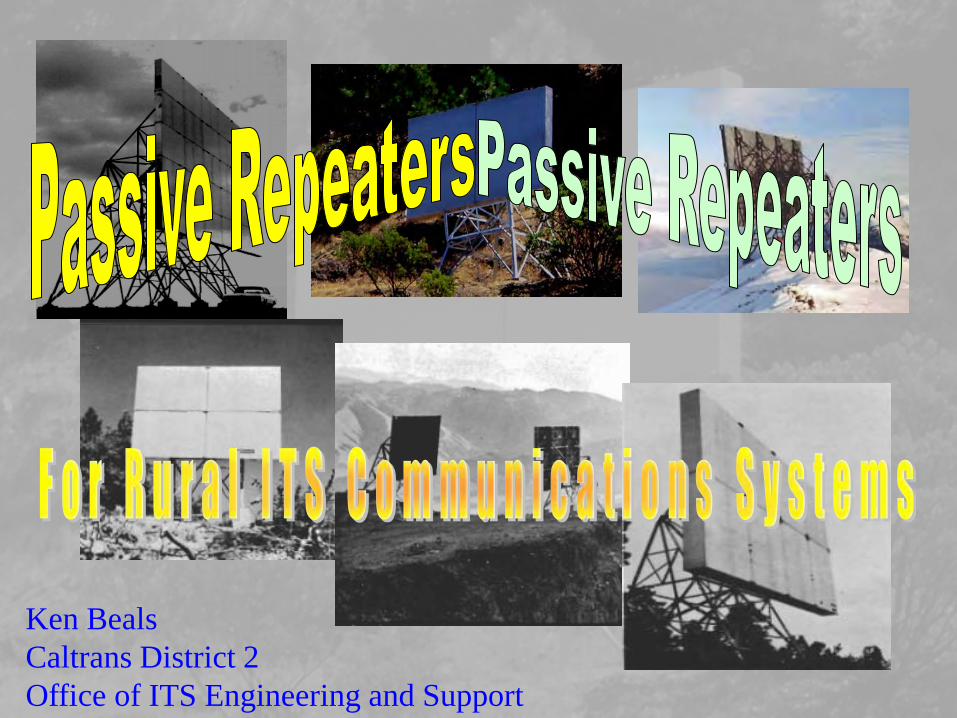
Ken BealsCaltrans District 2Office of ITS Engineering and Support

• The Concept

• History

• Identification of Locations

• Google Earth

• Visual Sighting

• Design Calculations

• Manual Calculation

• Excel Spreadsheet

• Design Software

Microwave Passive Repeater (Reflector) Design

• Design• Foundation• Plans

• Construction• Adjustment• Results• Summary• Thank You• Questions and Comments

Microwave Passive Repeater (Reflector) Design

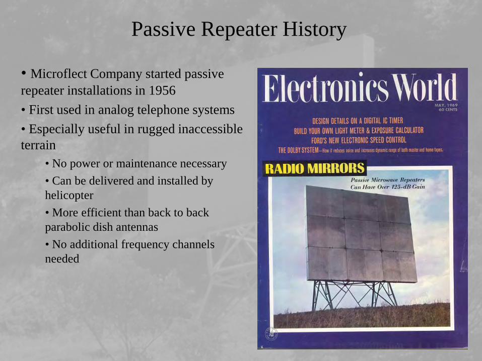
Passive Repeater History

• Microflect Company started passive repeater installations in 1956• First used in analog telephone systems• Especially useful in rugged inaccessible terrain

• No power or maintenance necessary• Can be delivered and installed by helicopter• More efficient than back to back parabolic dish antennas• No additional frequency channels needed

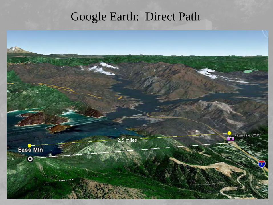
Google Earth: Direct Path

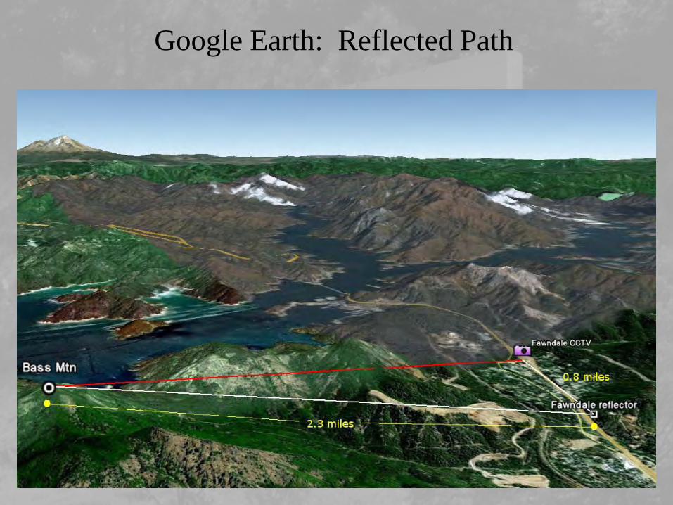
Google Earth: Reflected Path

Google Earth: Reflector Location

Visual Sighting: What do I look for?

• Visual Sighting• Simulation programs only show ground terrain.• Need to look for obstructions

• Vegetation• Buildings• Possible traffic obstructions

• Fresnel Zone• Volume surrounding line of

sight path between antennas.• Need to keep all

obstructions out of the Fresnel zone.

Visual Sighting: Fresnel Zone

• Fresnel Zone is a volume defined between the receive and transmit antennas.

• EM waves “spread out” from thetransmit antenna (HuygensPrinciple).• If some of the waves are blocked,the received signal will be reduced.

© Trevor Manning

Visual Sighting: Fresnel Zone• Additional signals can be caused by reflection and refraction off of objects in the path, and can add destructively at the receiver and reduce signal strength. Reflected signals undergo a 180° phase shift.

• Shape of the volume is an ellipsoid, since the sum of the distance between any point on the ellipsoid and both antennas (located at the foci of the ellipsoid) is a constant.

© Wikipedia

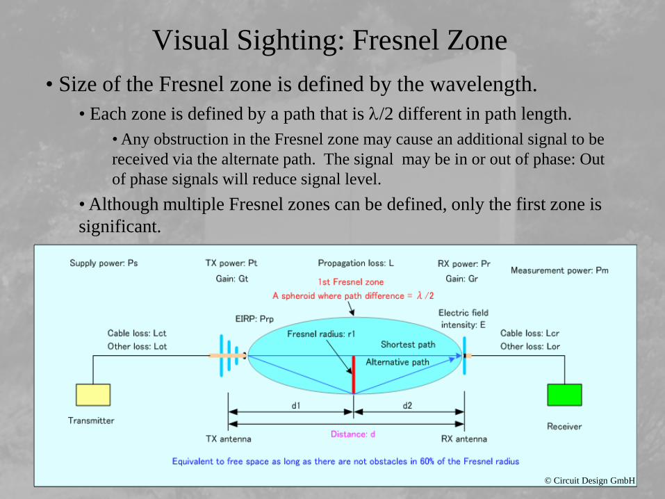
Visual Sighting: Fresnel Zone• Size of the Fresnel zone is defined by the wavelength.

• Each zone is defined by a path that is λ/2 different in path length.• Any obstruction in the Fresnel zone may cause an additional signal to be received via the alternate path. The signal may be in or out of phase: Out of phase signals will reduce signal level.

• Although multiple Fresnel zones can be defined, only the first zone is significant.

© Circuit Design GmbH

Visual Sighting: Fresnel Zone• The first Fresnel zone radius may be calculated using:

• There are two paths we need to look at:

• Reflector → Bass Mtn., Dist = 2.3 miles

• Reflector → Fawndale, Dist = 0.8 miles

GHz

mift freq

distr×

×=4

05.721

ftr ft 3.220.64

3.205.721 =×

×=

ftr ft 2.130.64

8.005.721 =×

×=

Visual Sighting: Fresnel Zone

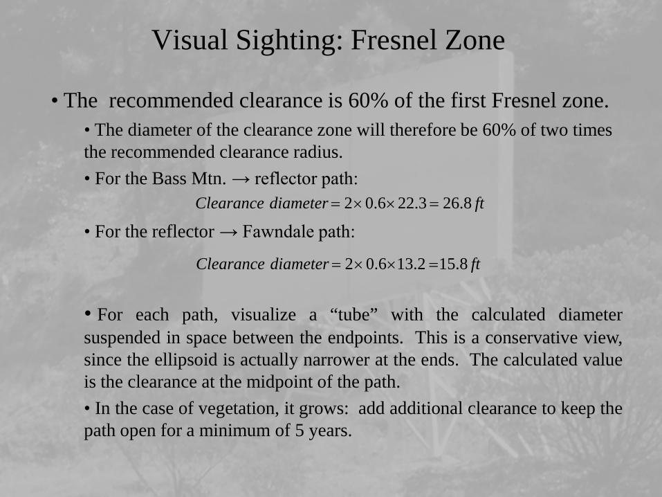
• The recommended clearance is 60% of the first Fresnel zone.• The diameter of the clearance zone will therefore be 60% of two times the recommended clearance radius.• For the Bass Mtn. → reflector path:

• For the reflector → Fawndale path:

• For each path, visualize a “tube” with the calculated diametersuspended in space between the endpoints. This is a conservative view,since the ellipsoid is actually narrower at the ends. The calculated valueis the clearance at the midpoint of the path.• In the case of vegetation, it grows: add additional clearance to keep thepath open for a minimum of 5 years.

ftdiameterClearance 8.263.226.02 =××=

ftdiameterClearance 8.152.136.02 =××=

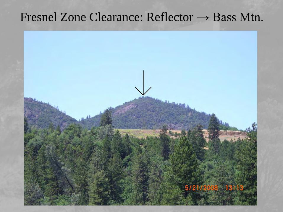
Fresnel Zone Clearance: Reflector → Bass Mtn.

Fresnel Zone Clearance: Reflector → Fawndale

© Valmont/Microflect Inc.

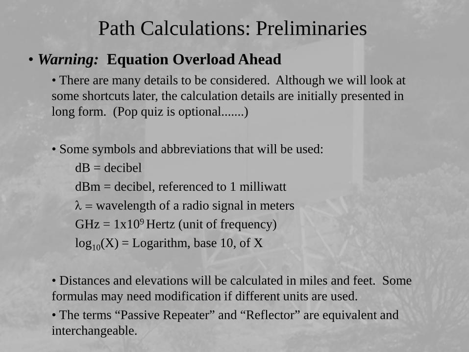
Path Calculations: Preliminaries• Warning: Equation Overload Ahead

• There are many details to be considered. Although we will look at some shortcuts later, the calculation details are initially presented in long form. (Pop quiz is optional.......)

• Some symbols and abbreviations that will be used:dB = decibeldBm = decibel, referenced to 1 milliwattλ = wavelength of a radio signal in metersGHz = 1x109 Hertz (unit of frequency) log10(X) = Logarithm, base 10, of X

• Distances and elevations will be calculated in miles and feet. Some formulas may need modification if different units are used.• The terms “Passive Repeater” and “Reflector” are equivalent and interchangeable.

Path Calculations: Preliminaries

• What do I need to know before beginning?• Where each location is located in 3D space:• Latitude, Longitude, Elevation.

• Accuracy is critical.• Handheld GPS is not “close enough” (especially for elevation).• Use a professional surveying team.

• Easily within ± 1 foot elevation, < 1 foot surface accuracy.

• From that information calculate:• Distance between points (accurate to 1 foot)• Elevation differences between points (accurate to 1 foot)• Horizontal angle between paths (two decimal places)• Vertical angles between reflector and end points (two decimal places)

• Correction for earth curvature can be calculated from:

5.1

2mi

ftDistCorrectionElevation =

Path Calculations: Vertical Angles

All elevations are to centerline of antenna/reflector

Path Calculations: Vertical Angles

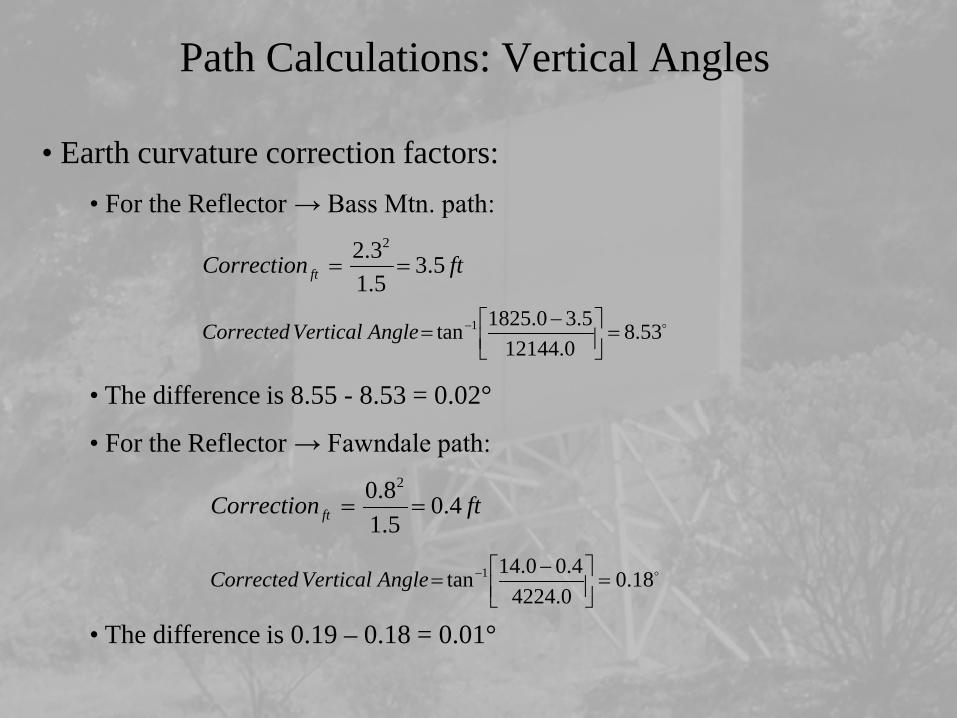
• Earth curvature correction factors:• For the Reflector → Bass Mtn. path:

• The difference is 8.55 - 8.53 = 0.02°

• For the Reflector → Fawndale path:

• The difference is 0.19 – 0.18 = 0.01°

ftCorrection ft 5.35.13.2 2

==

53.80.12144

5.30.1825tan 1 =

−

= −AngleVerticalCorrected

ftCorrection ft 4.05.18.0 2

==

18.00.4224

4.00.14tan 1 =

−

= −AngleVerticalCorrected

Path Calculations: Horizontal Angle• Find the bearing from the reflector to each end:

• Note: This formula calculates an angle from the ‘x’ axis in the Cartesian coordinate system. Compass bearings are referenced from North = 0°, so we will need to convert the angle to a compass bearing.

×∆

∆××−×= −

)cos()sin()cos()cos()sin()sin()cos(tan

2

21211

LatLongLongLatLatLatLatθ

Path Calculations: Horizontal Angle

• For the reflector to Bass Mtn. path:

• Correcting for the change of axis:

• For the reflector to Fawndale path:

• Correcting for the change of axis:

• The horizontal angle between the paths is:

48.64)7308.40cos()0063.0sin(

)0063.0cos()7308.40cos()7208.40sin()7308.40sin()7208.40cos(tan 1 =

×

××−×= −θ

42.21)7328.40cos()0404.0sin(

)0404.0cos()7328.40cos()7208.40sin()7328.40sin()7208.40cos(tan 1 −=

×−

−××−×= −θ

42.111)42.21(00.90 =−−=BearingCompass

52.2548.640.90 =−=BearingCompass

10.9452.25)18042.111(360 =++−

Path Calculations: Horizontal Angle• Let’s see what this looks like:

• Fade margin is the “extra” signal strength required at the receiver to allow for atmospheric and other conditions that cause variation in the received signal level.

• Several models are available for calculating fade margin. This model is known as the “Lenkurt” model, and tends to give the most conservative values.

Availability: relative uptime in the range of 0 – 1.0 (100% uptime = 1.0)TF = Terrain factorCF = Climate factorFreq = Frequency in GHzDist = Total path distance end to end in miles

Path Calculations: Fade Margin

××××

−−=

− 3510

410

1log10DistFreqCFTF

tyavailabiliFM

Path Calculations: Availability

© GTE Lenkurt Inc.

Path Calculations: Terrain/Climate Factor

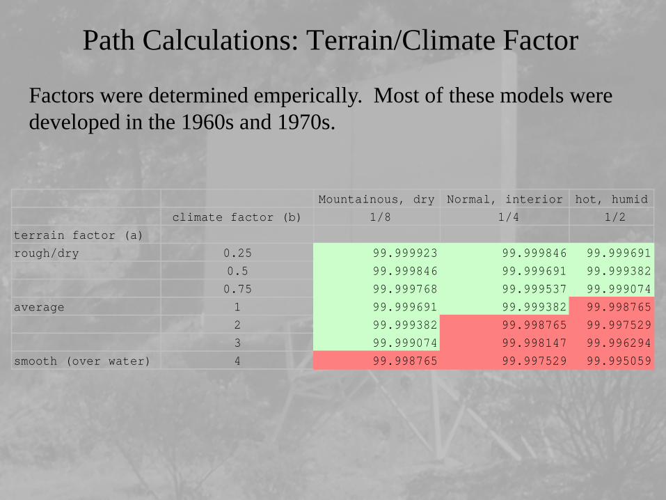
Factors were determined emperically. Most of these models were developed in the 1960s and 1970s.

Mountainous, dry Normal, interior hot, humidclimate factor (b) 1/8 1/4 1/2

terrain factor (a)rough/dry 0.25 99.999923 99.999846 99.999691

0.5 99.999846 99.999691 99.9993820.75 99.999768 99.999537 99.999074

average 1 99.999691 99.999382 99.9987652 99.999382 99.998765 99.9975293 99.999074 99.998147 99.996294

smooth (over water) 4 99.998765 99.997529 99.995059

• The fade margin formula assumes a single path, where we actually have two paths. The accepted industry standard is to calculate the fade margin over the single longer path.

The fade margin for the proposed link is calculated using the following factors:

Availability: 0.99999 (99.999%)Terrain factor = 1.0 (Average terrain)Climate factor = 0.250 (Normal interior climate)Distance = 3.1 milesFrequency = 6.0 GHz

The fade margin is added to the receiver threshold value to determine the required minimum received power level Pr.

Path Calculations: Fade Margin

dBFM 5.101.3

40.610250.00.1

99999.01log1035

10 =

××××

−−=

−

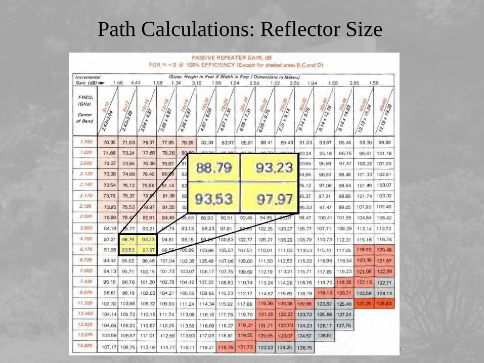
Path Calculations: Reflector Size• The required size of the reflector is determined by calculating the required gain of the reflector that will result in the necessary minimum signal at the receiver that was calculated earlier.

The path loss for each path is determing using a version of the Friis equation:

For the Reflector → Bass Mtn. path:

For the Reflector → Fawndale path:

)(log20)(log206.96 1010 MiGHzdB DistFreqPL ++=

dBPL 1.119)3.2(log20)0.6(log206.96 10101 =++=

dBPL 9.109)8.0(log20)0.6(log206.96 10102 =++=

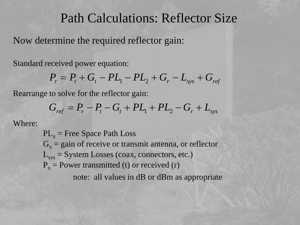
Path Calculations: Reflector SizeNow determine the required reflector gain:

Standard received power equation:

Rearrange to solve for the reflector gain:

Where:PLx = Free Space Path Loss Gx = gain of receive or transmit antenna, or reflectorLsys = System Losses (coax, connectors, etc.)Px = Power transmitted (t) or received (r)

note: all values in dB or dBm as appropriate

refsysrttr GLGPLPLGPP +−+−−+= 21

sysrttrref LGPLPLGPPG +−++−−= 21

Path Calculations: Reflector SizePlug in the numbers:

PL1 = 119.1 dBPL2 = 109.9 dBGx = 29.0 dB (Gain of transmit and receive antenna, each)Lsys = 12 dB (System losses (coax, connectors, etc.))Pt = +10 dBm (Transmitter power)Pr = -84.5 dBm (Receiver threshold + fade margin)

dBGref 5.880.120.299.1091.1190.290.105.84 =+−++−−−=

Path Calculations: Reflector Size


Reflector Gain

• Gain (in dB) or Directivity (a linear factor) can be determined directly from the effective aperture of an antenna. The aperture is the “capture area” of an antenna. It determines how much of the radiated EM plane wave power is intercepted by the antenna. • An isotropic antenna is one that receives or transmits equally well in all directions (in 3D space). Also known as a point source.

The effective aperture of an isotropic antenna is:and is considered the “reference” aperture.

Directivity (linear) or Gain (in dB) is defined as the ratio of the antenna aperture (or area) to the isotropic aperture.

πλ4

2

=

πλ4

log20 210ApertureGaindB

πλ4

2ApertureyDirectivit =

Reflector Gain

• Note that the “gain” of an antenna is completely independent of the physical shape.

• Antennas that look different can have the same gain:

dBiGain 8= dBiGain 8=

2048.0040.02.1

mAreamWidth

mLength

=

==

2047.0216.0

216.0

mAreamWidth

mLength

=

==

© L-com © L-com.

Reflector Gain

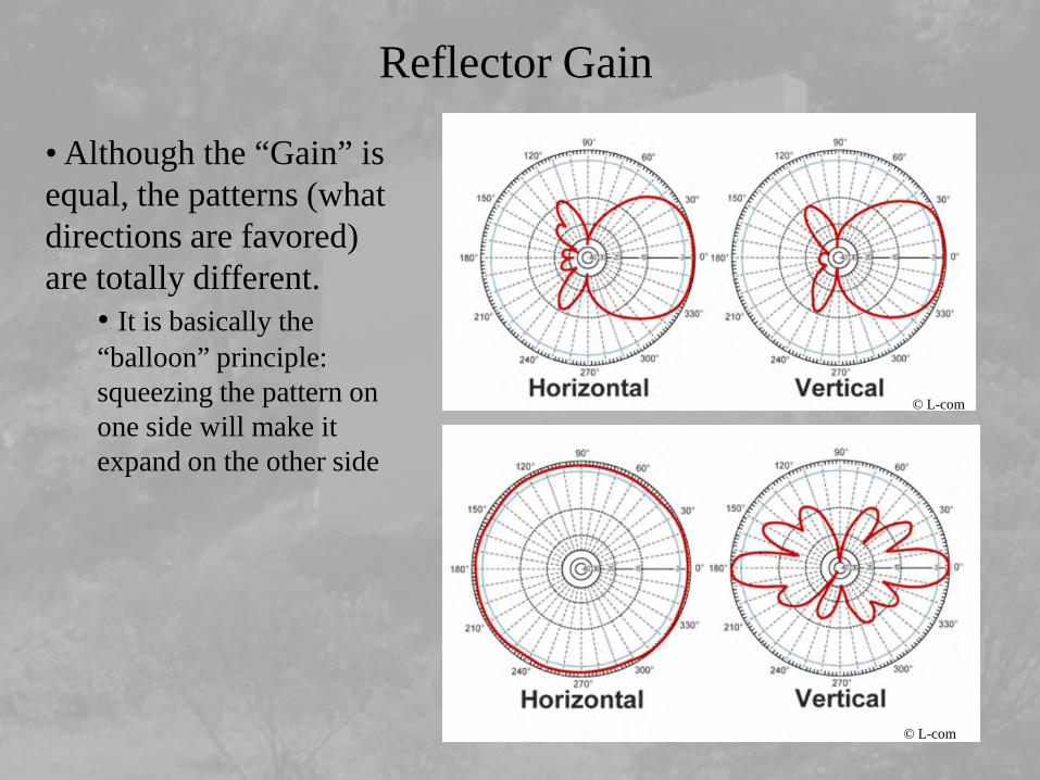
• Although the “Gain” is equal, the patterns (what directions are favored) are totally different.

• It is basically the “balloon” principle: squeezing the pattern on one side will make it expand on the other side

© L-com

© L-com

Reflector Gain

• For the reflector, gain will be the ratio of the aperture of the reflector (physical area) to the isotropic aperture:

A 16’ x 10’ reflector (4.88 m x 3.05 m) operated at 6.0 GHz has a gain of:

Note that this gain is only at the wavelength specifiedLower frequencies ( larger λ) means lower gainAt 2.4 GHz, the reflector would have to be 40’ x 25’ for the same gain

*It just so happens that this is the reflector size used for this project.

dBGref 5.97

405.0

05.388.4log20 210 =

×

=

π

Reflector Gain

Problem: This is the gain of the reflector with the EM wave normal to the reflector face:

What happens when the waves are not normal to the surface?

Reflector GainReflector Effective Area: Look at three cases:

Waves normal to the surface:Effective Area = Reflector area

Waves intersect at an angle to the normal:Effective area = some fraction of the Reflector area

Waves intersect at 90° to the normal:Effective area = 0

Reflector GainThe result is what you would expect:Reflector effective area = Area * cos(wave intercept angle)

By the law of reflection, we know that the angle of the incoming wave and the angle of the outgoingwave are equal with respect to the normal of the surface.

Since we have already calculated the angle between the paths, the intercept angle is simply one-half of the included angle.

The wave intercept angle is given the symbol α, and the included angle is therefore 2α.

For the 16’x10’ (4.88 m x 3.05 m) reflector used in this design:

And the gain is now:214.10)05.47cos(88.14 mAeffective =°×=

dBGref 41.94

405.014.10log20 210 =

=

π

Reflector Gain DetailsSome details:

• Antennas normally have an “efficiency” factor.• Reflector efficiency is generally 100%

• The reflector has no conduction or dielectric loss • There are some effects related to surface flatness for very large reflectors operated at very high frequencies (10 GHz and above). These effects can reduce the gain by up to 3 dB worst case.

• The “true” included angle.• The incident wave angle α is technically one-half of the horizontal angle corrected by an additional value due to the vertical angles between the paths. For vertical angles > 20°, the “true” included angle must be calculated and used to determine the reflector gain. The plane defined by the paths between the endpoints and the reflector is not horizontal: it is tilted. The actual angle (as seen from the reflector) is different from the angle as measured in the horizontal plane. For small vertical angles, the correction is small (as we shall see).

Reflector Gain Details• Antenna gain is normally specified at the “far field” distance.

• If the reflector is too close to a receive or transmit antenna, gain will be affected. In the “near field” region, interaction between the antenna and reflector cause the net gain to be reduced.• For reflectors and antennas in their “near field” zones, a correction factor must be applied.• Near/far field can be determined by:

A = Reflector area in sq. feetd = distance between antenna and reflector in feetα = wave intercept angle λ = wavelength in feet

• If then antenna and reflector are in far field.

Tables and formulas are available to determine correction factor.

• For this project: so the reflector is in far field.

effAd

k ×××

=4

1 λπ αcosAeffA =

5.21≥

k

99.41094

4224164.01=

×××

=π

k

Reflector Gain Details• Polarization rotation

• Polarization is the alignment of the E and H fields of the electromagnetic wave with respect to a reference (the earth’s surface being common).• The polarization must be the same at the transmitter and receiver for the maximum signal to be transferred.• EM waves reflected from a flat surface under certain conditions will undergo a rotation of polarization. If the shift is significant, additional attenuation will occur.• If the polarization rotation is significant, it can easily be corrected by rotating one of the antennas.• Polarization rotation increases as the angles (both horizontal and vertical) from the reflector to the endpoints increases.• Polarization rotation and attenuation is calculated after the final reflector position angles are determined.

Reflector gain: Large Horizontal AngleAs we observed earlier, as the included angle increases, the gain of the reflector is decreased due to the decreased effective area. Using our 16’x10’ (4.88 x 3.05 m) reflector as an example:

When α = 65° (included angle 130°) :

The gain of the reflector is now:

Compared to the 0° angle gain we calculated earlier:

Therefore: once the included angle exceeds 130°, the path needs to be changed to reduce the reflection angles.

dBGref 0.90

405.029.6log20 210 =

=

π

229.6)65cos()05.388.4( mAreaEffective =××=

dBdBdB 5.75.970.90 −=−

Reflector gain: Large Horizontal AngleFor large horizontal angles, a double reflector is used.

The possibilities are endless:

© Valmont/Microflect Inc. © Valmont/Microflect Inc.

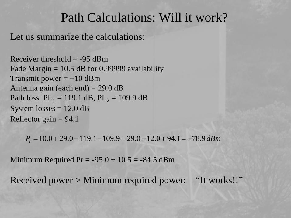
Path Calculations: Will it work?Let us summarize the calculations:

Receiver threshold = -95 dBmFade Margin = 10.5 dB for 0.99999 availabilityTransmit power = +10 dBmAntenna gain (each end) = 29.0 dBPath loss PL1 = 119.1 dB, PL2 = 109.9 dBSystem losses = 12.0 dBReflector gain = 94.1

Minimum Required Pr = -95.0 + 10.5 = -84.5 dBm

Received power > Minimum required power: “It works!!”

dBmPr 9.781.940.120.299.1091.1190.290.10 −=+−+−−+=

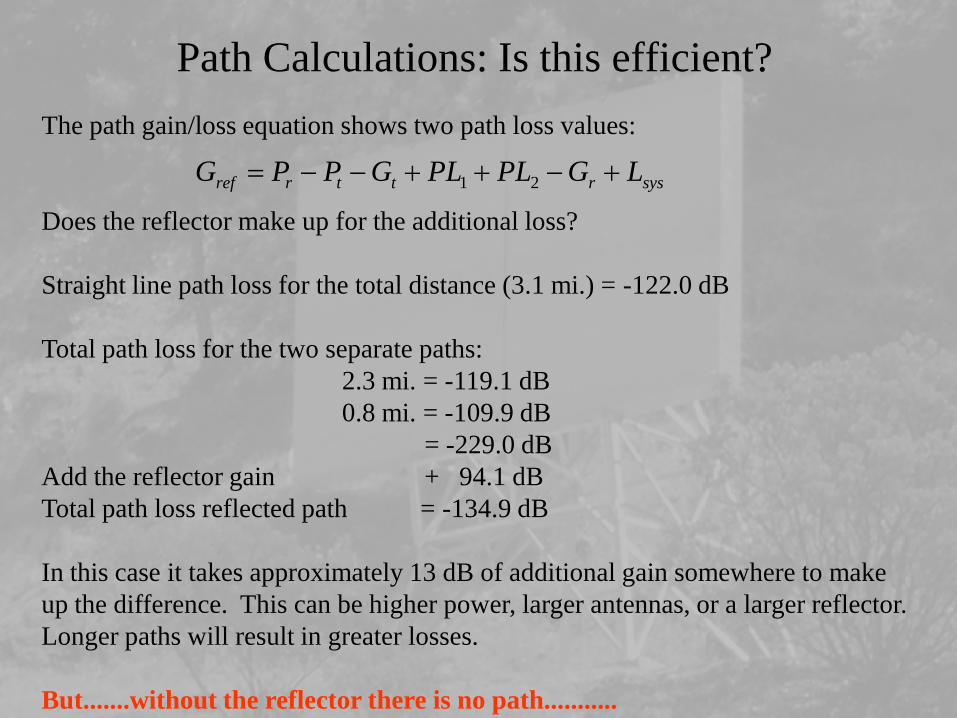
Path Calculations: Is this efficient?The path gain/loss equation shows two path loss values:

Does the reflector make up for the additional loss?

Straight line path loss for the total distance (3.1 mi.) = -122.0 dB

Total path loss for the two separate paths:2.3 mi. = -119.1 dB0.8 mi. = -109.9 dB

= -229.0 dBAdd the reflector gain + 94.1 dBTotal path loss reflected path = -134.9 dB

In this case it takes approximately 13 dB of additional gain somewhere to make up the difference. This can be higher power, larger antennas, or a larger reflector. Longer paths will result in greater losses.

But.......without the reflector there is no path...........

sysrttrref LGPLPLGPPG +−++−−= 21

ReflectorPosition

Calculations

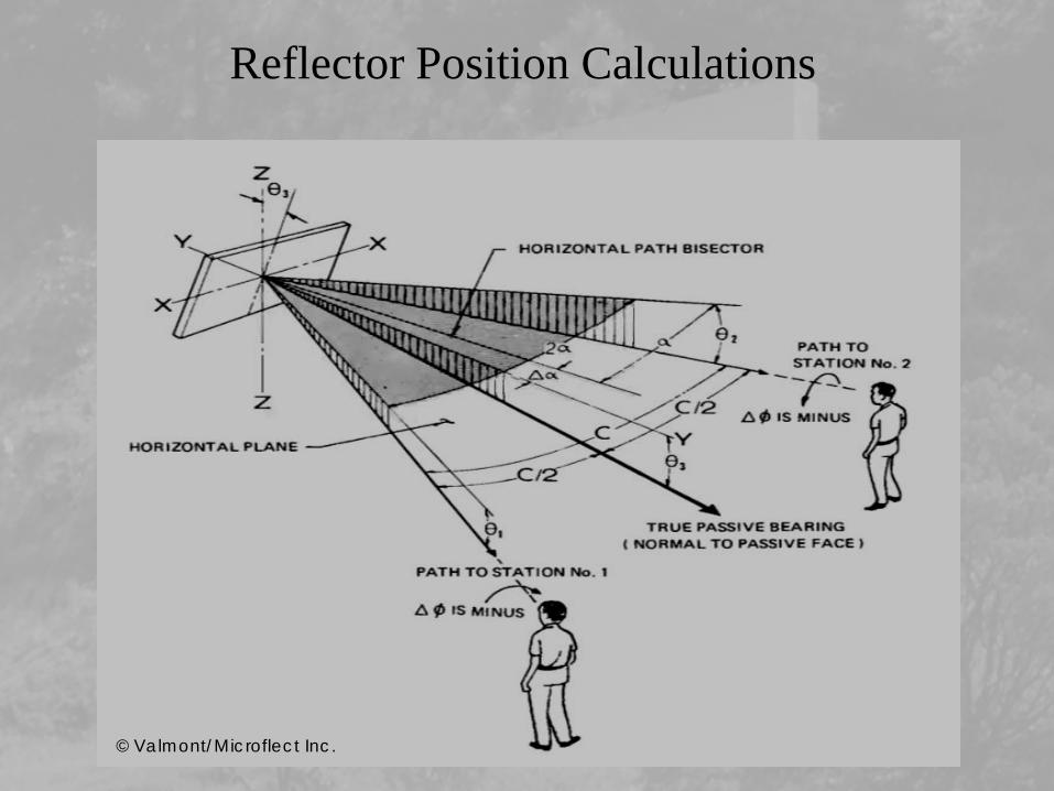
Reflector Position Calculations• How do we determine the physical position of the reflector?

• Theory: the normal to the face of the reflector must bisect the true angle between the two endpoints.

• Start with the horizontal angle between the sites.• Calculate the correction to the horizontal angle to compensate for the tilt of the plane containing the paths.• Calculate the necessary vertical angle of the reflector face.

• The equations:

θ1 = smaller of the two vertical angles to endpointsθ2 = larger of the two vertical angles to endpointsθ3 = vertical tilt of the reflectorα = ½ of the horizontal angle between the endpoints∆α = correction to the horizontal angle

21

21

coscoscoscostantan

θθθθαα

+−

×=∆21

213 coscos

sinsincos

costanθθθθ

ααθ

+−

×∆

=

Reflector Position Calculations


Reflector Position Calculations

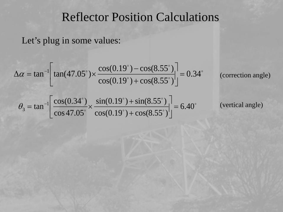
Let’s plug in some values:

(correction angle)

(vertical angle)

34.0

)55.8cos()19.0cos()55.8cos()19.0cos()05.47tan(tan 1 =

+−

×=∆ −α

40.6)55.8cos()19.0cos()55.8sin()19.0sin(

05.47cos)34.0cos(tan 1

3 =

++

×= −θ

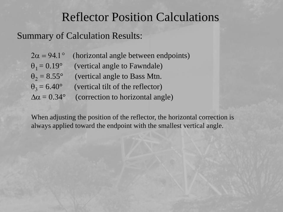
Reflector Position CalculationsSummary of Calculation Results:

2α = 94.1° (horizontal angle between endpoints)θ1 = 0.19° (vertical angle to Fawndale)θ2 = 8.55° (vertical angle to Bass Mtn.θ3 = 6.40° (vertical tilt of the reflector)∆α = 0.34° (correction to horizontal angle)

When adjusting the position of the reflector, the horizontal correction is always applied toward the endpoint with the smallest vertical angle.

Reflector Position Calculations• Polarization rotation (just for drill)

• We know polarization rotation is likely to be insignificant due to the small vertical angles.• The relevant equations are:

True angle between endpoints, C:

θ1, θ2 = vertical angles to endpointsθ3 = reflector vertical angle

Rotation of wave at each end:

φ1, φ2 = polarization rotationat endpoint

∆φ = total rotation over the path

Total rotation of wave over the path:

×

×−= −

CC

sincoscossinsincos

2

2111 θ

θθφ

×

×−= −

2sincos

2cossinsin

cos1

131

2 C

C

θ

θθφ

18021 −+=∆ φφφ

×

+×= −

3

211

sin2sinsincos2θ

θθC

Reflector Position Calculations• Some numbers:

(was 94.10°)

Attenuation due to polarization rotation:

21.89)03.94sin()55.8cos(

)03.94cos()55.8sin()19.0sin(cos 1 =×

×−=φ

47.918032.8121.89 −=−+=∆φ

( )210 cos1log10

φ∆=dBLoss

( ) dBLossdB 12.0)47.9cos(

1log10 210 =−

=

03.94)40.6sin(2

)55.8sin()19.0sin(cos2 1 =

×

+×= −C

32.81)19.0cos()01.47sin(

)19.0sin()01.47cos()40.6sin(cos 2 =×

×−=φ

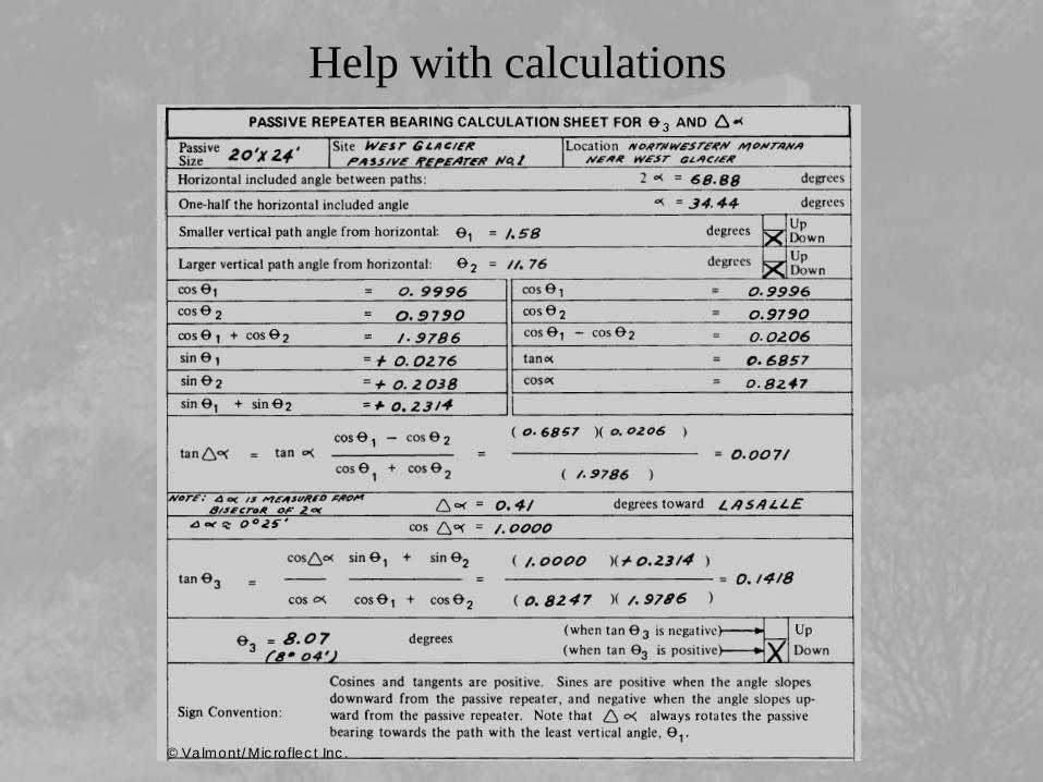
Help with calculations

• This is a well developed and tested technology (no magic)

• Valmont/Microflect manual provides everything you need to know to successfully implement a reflector• Worksheets with examples• Tables and graphs to select the proper size• Available on the web







There must be an easier way.......

• There is no shortcut to the field work.• Google Earth helps, but there is no substitute for physically sighting the path.

• Two options for use of present technology• Excel-type spreadsheet.

• Enter the formulas and data manually• Need a way to validate results.

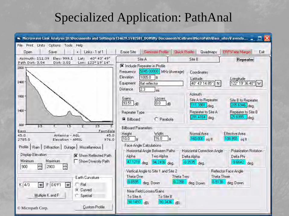
• Specialized Application• (Hopefully) well tested.• Extra features such as terrain identification• Up and running with a minimum of time investment.

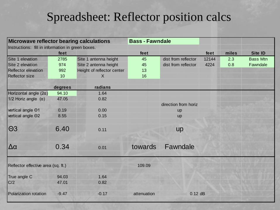
Spreadsheet: Reflector position calcs

Microwave reflector bearing calculations Bass - FawndaleInstructions: fill in information in green boxes.

feet feet feet miles Site IDSite 1 elevation 2785 Site 1 antenna height 45 dist from reflector 12144 2.3 Bass MtnSite 2 elevation 974 Site 2 antenna height 45 dist from reflector 4224 0.8 FawndaleReflector elevation 992 Height of reflector center 13Reflector size 10 X 16

degrees radiansHorizontal angle (2α) 94.10 1.641/2 Horiz angle (α) 47.05 0.82

direction from horizvertical angle Θ1 0.19 0.00 upvertical angle Θ2 8.55 0.15 up

Θ3 6.40 0.11 up

Δα 0.34 0.01 towards Fawndale

Reflector effective area (sq. ft.) 109.09

True angle C 94.03 1.64C/2 47.01 0.82

Polarization rotation -9.47 -0.17 attenuation 0.12 dB

Spreadsheet: Fade MarginMicrowave path calculations Microwave path availability vs. terrain and conditions variablesA(dB)=96.6 + 20logF(GHz)+20logD(Mi) Undp = b * a * 10E-5 * (f/4) * D^3 * 10^(-F/10)

path: Bass - Fawndale (via reflector)

link dist (D1): 2.3 miles Mountainous, dry Normal, interior hot, humidlink dist (D2) 0.8 miles climate factor (b) 1/8 1/4 1/2Freq (f): 5.8 GHz terrain factor (a)Tx pwr 10 dBm rough/dry 0.25 99.999967 99.999933 99.999866Rx thres -95 dBm 0.5 99.999933 99.999866 99.999733

0.75 99.999900 99.999800 99.999599Path 1 loss -119.1 dB average 1 99.999866 99.999733 99.999466Reflector gain 94.1 dB size= 10x16 2 99.999733 99.999466 99.998931Path 2 loss -109.9 dB 3 99.999599 99.999199 99.998397Total path loss -134.9 smooth (over water) 4 99.999466 99.998931 99.997863

Tx TL 5.00 dBTx jumpers 0.50 dB seconds/year total 31536000 1/8 1/4 1/2Tx connectors 0.50 dB seconds/year outage 0.25 10.53 21.06 42.12Rx connectors 0.50 dB 0.5 21.06 42.12 84.25Rx jumpers 0.50 dB 0.75 31.59 63.18 126.37Rx TL 5.00 dB 1 42.12 84.25 168.49misc/safety 0.00 dB 2 84.25 168.49 336.98

3 126.37 252.74 505.47Antenna gain 29.00 dB 4 168.49 336.98 673.96

Total gain 68 minutes/year outage 0.25 0.18 0.35 0.70Total loss -146.93 0.5 0.35 0.70 1.40

0.75 0.53 1.05 2.11Receive Sig -78.93 1 0.70 1.40 2.81Fade Margin (F) 16.07 2 1.40 2.81 5.62

3 2.11 4.21 8.424 2.81 5.62 11.23

Specialized Application: PathAnal

© Micropath Corp.


© Micropath Corp.


© Micropath Corp.


© Micropath Corp.

The Physical StuffWe have everything we need on paper, but it is only useful if it exists in the real world......

Everything Begins with a Good Foundation



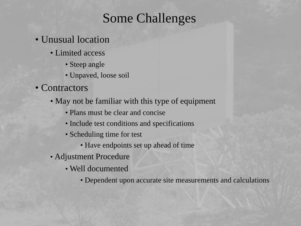
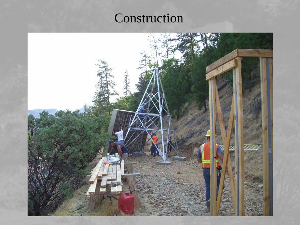
Some Challenges• Unusual location

• Limited access• Steep angle• Unpaved, loose soil

• Contractors• May not be familiar with this type of equipment

• Plans must be clear and concise• Include test conditions and specifications• Scheduling time for test

• Have endpoints set up ahead of time• Adjustment Procedure

• Well documented• Dependent upon accurate site measurements and calculations

Construction

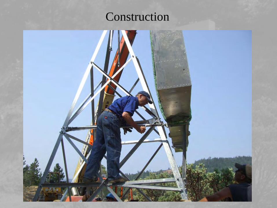
Construction

Construction

Construction

Construction

Construction

Construction

Adjustment: Equipment

• Use of transit/theodolite with digital readout

• Measures horizontal and vertical angles• Allows measurement of differences on each side of center

• Adjustment “sticks” attached to reflector

• Provides measurement from each corner of the reflector

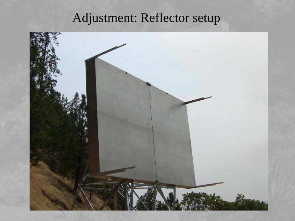
Adjustment: Reflector setup

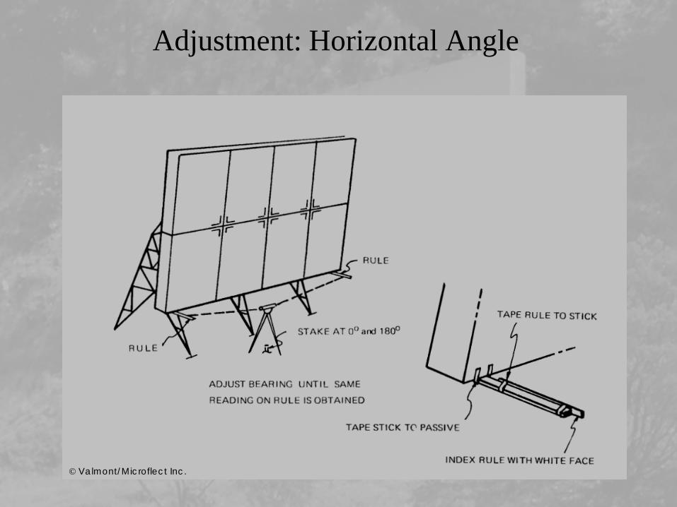
Adjustment: Horizontal Angle


Adjustment: Horizontal Angle Correction

Total difference between readings = 1.14”

"57.0)34.0tan(128 =××= x

Adjustment: Vertical angle

"5.1340.6tan"12'10 =××= x)( longerisstickUpper

( )up40.63 =θ


Adjustment: Mechanics• Lower adjustment rods used for both horizontal and vertical adjustment

• Upper arms are attached after final position is set.• Adjustment range is limited

• Foundation location is critical

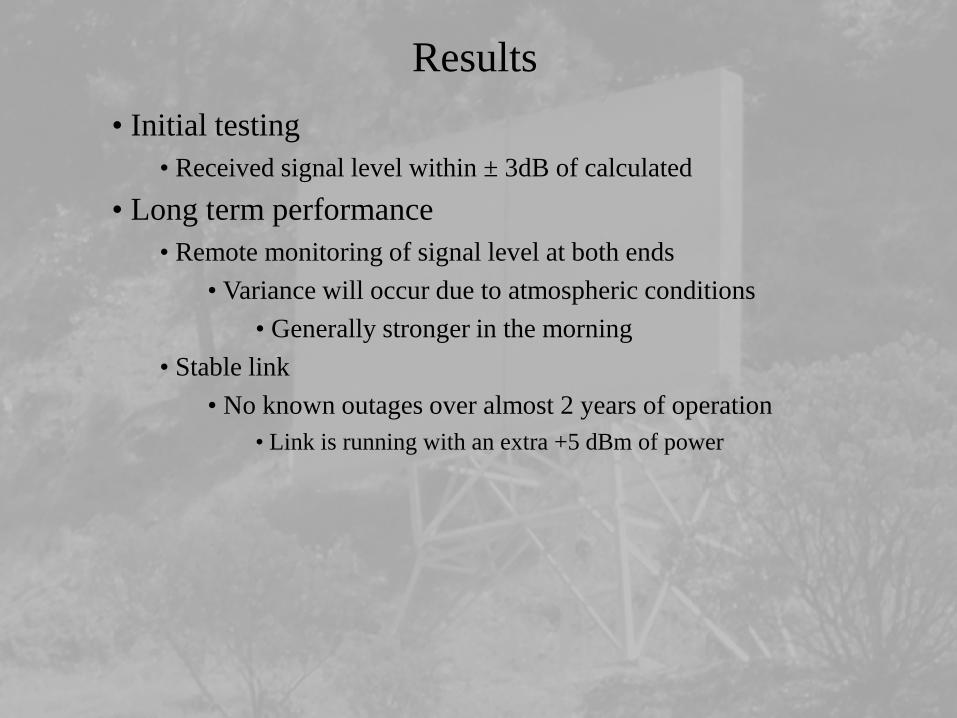
Results• Initial testing

• Received signal level within ± 3dB of calculated• Long term performance

• Remote monitoring of signal level at both ends• Variance will occur due to atmospheric conditions

• Generally stronger in the morning• Stable link

• No known outages over almost 2 years of operation• Link is running with an extra +5 dBm of power

Results: Signal Strength

Results: Signal Strength

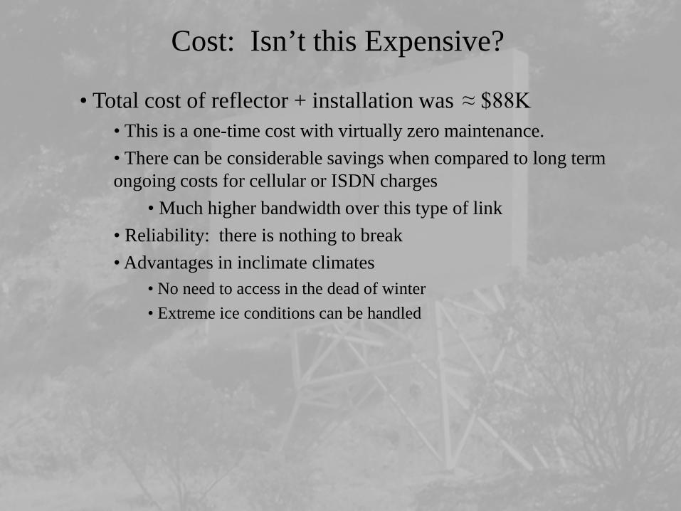
Cost: Isn’t this Expensive?

• Total cost of reflector + installation was ≈ $88K• This is a one-time cost with virtually zero maintenance.• There can be considerable savings when compared to long term ongoing costs for cellular or ISDN charges

• Much higher bandwidth over this type of link• Reliability: there is nothing to break• Advantages in inclimate climates

• No need to access in the dead of winter• Extreme ice conditions can be handled

Summary

• Just because a remote site is not within “line of sight” does not mean it cannot be accessed via microwave radio.

• Highways tend to be in canyons• Right of way many times will include locations well above the roadway level• A reflector can be put in locations that would be impractical for an “active” repeater

• No power required• No maintenance or repair• No regular access needs to be maintained• Reliability of the passive repeater, properly installed, will be 100%

Thank You

• Every project requires the support of lots of folks, without whose assistance no project would be successful.

• Caltrans• Art Robles, P.E., Caltrans Electrical Design• Mike Mogen P.E., Caltrans Civil Engineering Design• Gary Meurer, Caltrans ITS Electronic Technician• Ian Turnbull, P.E., Chief, Office of ITS Engineering and Support• Ken Vomaske, P.E., Caltrans Construction

• Contractors and Suppliers• Valmont/Microflect Inc. (Supplier)• Schommer & Sons (Installation contractor)

Questions & Comments

?

Documents

Ken Beals Caltrans District 2 Office of ITS Engineering and Support