Az optimalizációs és regressziós feladat zajérzékenysége – véletlen mátrixok és replikák alkalmazása

Kondor ImreCollegium Budapest és ELTE

Rendezetlen rendszerekELTE, 2007/08 II. félév

Contents

• I. Preliminaries

the problem of noise, risk measures, noisy covariance matrices

• II. Random matrices

Spectral properties of Wigner and Wishart matrices

• III. Beyond the stationary, Gaussian world

non-stationary case, alternative risk measures (mean absolute deviation, expected shortfall, worst loss), their sensitivity to noise, the feasibility problem

I. PRELIMINARIES

PortfoliosConsider a linear combination of returns

with weights : . The weights add up to unity: . The portfolio’s expectation value is: with variance:

where is the covariance matrix, the standard deviation of return , and the correlation matrix.

ir

iw1ii

w P i ii

w 2P i ij j

i j

w w

P i iir w r

i irijjiij C

ijC

Level surfaces of risk measured in variance

• The covariance matrix is positive definite. It follows that the level surfaces (iso-risk surfaces) of variance are (hyper)ellipsoids in the space of weights. The convex iso-risk surfaces reflect the fact that the variance is a convex measure.

• The principal axes are inversely proportional to the square root of the eigenvalues of the covariance matrix.

Small eigenvalues thus correspond to long axes.• The risk free asset would correspond to an infinite

axis, and the correspondig ellipsoid would be deformed into an elliptical cylinder.

The Markowitz problem

• According to Markowitz’ classical theory the tradeoff between risk and reward can be realized by minimizing the variance

over the weights, for a given expected return

and budget

2P i ij j

i j

w w

1ii

w

i ii

w

• Geometrically, this means that we have to blow up the risk ellipsoid until it touches the intersection of the two planes corresponding to the return and budget constraints, respectively. The point of tangency is the solution to the problem.

• As the solution is the point of tangency of a convex surface with a linear one, the solution is unique.

• There is a certain continuity or stability in the solution: A small miss-specification of the risk ellipsoid leads to a small shift in the solution.

• Covariance matrices corresponding to real markets tend to have mostly positive elements.

• A large, complicated matrix with nonzero average elements will have a large (Frobenius-Perron) eigenvalue, with the corresponding eigenvector having all positive components. This will be the direction of the shortest principal axis of the risk ellipsoid.

• Then the solution also will have all positive components. Fluctuations in the small eigenvalue sectors may have a relatively mild effect on the solution.

The minimal risk portfolio• Expected returns are hardly possible (on

efficient markets, impossible) to determine with any precision.

• In order to get rid of the uncertainties in the returns, we confine ourselves to considering the minimal risk portfolio only, that is, for the sake of simplicity, we drop the return constraint.

• Minimizing the variance of a portfolio without considering return does not, in general, make much sense. In some cases (index tracking, benchmarking), however, this is precisely what one has to do.

The weights of the minimal risk portfolio

• Analytically, the minimal variance portfolio corresponds to the weights for which

is minimal, given .

The solution is: .

• Geometrically, the minimal risk portfolio is the point of tangency between the risk ellipsoid and the plane of he budget constraint.

2P i ij j

i j

w w

1ii

w 1

*1

ijji

jkj k

w

Empirical covariance matrices• The covariance matrix has to be determined from

measurements on the market. From the returns observed at time t we get the estimator:

• For a portfolio of N assets the covariance matrix has O(N²) elements. The time series of length T for N assets contain NT data. In order for the measurement be precise, we need N <<T. Bank portfolios may contain hundreds of assets, and it is hardly meaningful to use time series longer than 4 years (T~1000). Therefore, N/T << 1 rarely holds in practice. As a result, there will be a lot of noise in the estimate, and the error will scale in N/T.

(1) 1

1

T

ij it jtTt

y y

An intriguing observation• L.Laloux, P. Cizeau, J.-P. Bouchaud, M. Potters,

PRL 83 1467 (1999) and Risk 12 No.3, 69 (1999)

and

V. Plerou, P. Gopikrishnan, B. Rosenow, L.A.N. Amaral, H.E. Stanley, PRL 83 1471 (1999)

noted that there is such a huge amount of noise in empirical covariance matrices that it may be enough to make them useless.

• A paradox: Covariance matrices are in widespread use and banks still survive ?!

Laloux et al. 1999

The spectrum of the covariance matrix obtained from the timeseries of S&P 500with N=406, T=1308, i.e. N/T= 0.31, compared with that of a completely random matrix (solid curve). Only about 6% of the eigenvalues lie beyond the random band.

Remarks on the paradox• The number of junk eigenvalues may not

necessarily be a proper measure of the effect of noise: The small eigenvalues and their eigenvectors fluctuate a lot, indeed, but perhaps they have a relatively minor effect on the optimal portfolio, whereas the large eigenvalues and their eigenvectors are fairly stable.

• The investigated portfolio was too large compared with the length of the time series.

• Working with real, empirical data, it is hard to distinguish the effect of insufficient information from other parasitic effects, like nonstationarity.

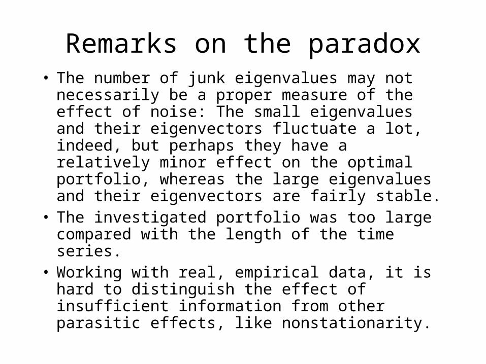
A historical remark• Random matrices first appeared in a finance context

in G. Galluccio, J.-P. Bouchaud, M. Potters, Physica A 259 449 (1998). In this paper they show that the optimization of a margin account (where, due to the obligatory deposit proportional to the absolute value of the positions, a nonlinear constraint replaces the budget constraint) is equivalent to finding the ground state configuration of what is called a spin glass in statistical physics. This task is known to be NP-complete, with an exponentially large number of solutions.

• Problems of a similar structure would appear if one wanted to optimize the capital requirement of a bond portfolio under the rules stipulated by the Capital Adequacy Directive of the EU (see below)

A filtering procedure suggested by RMT• The appearence of random matrices in the context of

portfolio selection triggered a lot of activity, mainly among physicists. Laloux et al. and Plerou et al. proposed a filtering method based on random matrix theory (RMT) subsequently. This has been further developed and refined by many workers.

• The proposed filtering consists basically in discarding as pure noise that part of the spectrum that falls below the upper edge of the random spectrum. Information is carried only by the eigenvalues and their eigenvectors above this edge. Optimization should be carried out by projecting onto the subspace of large eigenvalues, and replacing the small ones by a constant chosen so as to preserve the trace. This would then drastically reduce the effective dimensionality of the problem.

• Interpretation of the large eigenvalues: The largest one is the „market”, the other big eigenvalues correspond to the main industrial sectors.

• The method can be regarded as a systematic version of principal component analysis, with an objective criterion on the number of principal components.

• In order to better understand this novel filtering method, we have to recall a few results from Random Matrix Theory (RMT)

II. RANDOM MATRICES

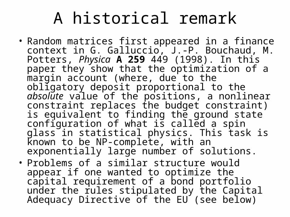
Origins of random matrix theory (RMT)• Wigner, Dyson 1950’s• Originally meant to describe (to a zeroth approximation)

the spectral properties of heavy atomic nuclei - on the grounds that something that is sufficiently complex is almost random- fits into the picture of a complex system, as one with a large number of degrees of freedom, without symmetries, hence irreducible, quasi random. - markets, by the way, are considered stochastic for similar reasons

• Later found applications in a wide range of problems, from quantum gravity through quantum chaos, mesoscopics, random systems, etc. etc.

RMT

• Has developed into a rich field with a huge set of results for the spectral properties of various classes of random matrices

• They can be thought of as a set of „central limit theorems” for matrices

Wigner semi-circle law

• Mij symmetrical NxN matrix with i.i.d. elements (the distribution has 0 mean and finite second moment)

• k: eigenvalues of

• The density of eigenvalues k (normed by N) goes to the Wigner semi-circle for N→∞ with prob. 1:

,

, otherwise

2 22

1( ) 4

2x x

| | 2x

( ) 0x

N

M ji ,

Remarks on the semi-circle law

• Can be proved by the method of moments (as done originally by Wigner) or by the resolvent method (Marchenko and Pastur and countless others)

• Holds also for slightly dependent or non-homogeneous entries (e.g. for the association matrix in networks theory)

• The convergence is fast (believed to be of ~1/N, but proved only at a lower rate), especially what concerns the support

Convergence to the semi-circle as N increases

Elements of M are distributed normally

N=20

N=50

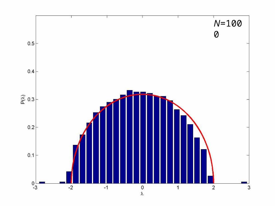
N=100

N=200

N=500

N=1000

If the matrix elements are not centered but have, say, a common mean, one large eigenvalue breaks away, the rest stay in the semi-circle

If the matrix elements are not centered N=1000

N=1000

For fat-tailed (but finite variance) distributions the theorem still holds, but the convergence is slow

Sample from Student t (freedom=3) distribution

N=20

N=50

N=100

N=200

N=500

N=1000

There is a lot of fluctuation, level crossing, random rotation of eigenvectors taking place in the bulk

Illustration of the instability of the eigenvectors, although the distribution of the eigenvalues is the same.

Sample 1

Matrix elements normally distributed

N=1000

Sample 2

Sample k

Scalar product of the eigenvectors assigned to the j. eigenvalue of the matrix.

The eigenvector belonging to the large eigenvalue (when there is one) is much more stable. The larger the eigenvalue, the more so.

Illustration of the stability of the largest eigenvectorSample 1Matrix elements are normally distributed, but the sum of the elements in the rows is not zero.N=1000

Sample 2

Sample k

Scalar product of the eigenvectors belonging to the largest eigenvalue of the matrix. The larger the first eigenvalue, the closer the scalar products to 1 or -1.

The eigenvector components

• A lot less is known about the eigenvectors.

• Those in the bulk have random components

• The one belonging to the large eigenvalue (when there is one) is completely delocalized

Wishart matrices – random sample covariance matrices

• Let Aij be an N x T matrix with i.i.d. elements (0 mean and finite second moment)

• σ =1/T AA’ where A’ is the transpose

• Wishart or Marchenko-Pastur spectrum (eigenvalue distribution):

where( )( )

( )2

min maxT

N

2

1 Nmax min T

Remarks• The theorem also holds when E{A} is of finite

rank• The assumption that the entries are identically

distributed is not necessary• If T < N the distribution is the same with and extra

point of mass 1 – T/N at the origin• If T = N the Marchenko-Pastur law is the squared

Wigner semi-circle• The proof extends to slightly dependent and

inhomogeneous entries• The convergence is fast, believed to be of ~1/N ,

but proved only at a lower rate

Convergence in N, with T/N = 2 fixed

The red curve is the limit Wishart distribution

N=20

T/N=2

N=50

T/N=2

N=100

T/N=2

N=200

T/N=2

N=500

T/N=2

N=1000

T/N=2

Evolution of the distribution with T/N, with N = 1000 fixed

The quadratic limit N=1000

T/N=1

N=1000

T/N=1.2

N=1000

T/N=2

N=1000

T/N=3

N=1000

T/N=5

N=1000

T/N=10

Scalar product of the eigenvectors belonging to the j eigenvalue of the matrices for different samples.

Eigenvector components

The same applies as in the Wigner case: the eigenvectors in the bulk are random, the one outside is delocalized

Distribution of the eigenvector components, if no dominant eigenvalue exists.

N=100T/N=2Rho=0.1

Market model

Underlying distribution is Wishart

N=200T/N=2

N=500T/N=2

N=1000T/N=2

Scalar product of the eigenvectors belonging to the largest eigenvalue of the matrix. The larger the first eigenvalue, the closer the scalar products to 1.

III. OUT OF SAMPLE ESTIMATION ERROR

Some key points

Laloux et al. and Plerou et al. demonstrate the effect of noise on the spectrum of the correlation matrix C. This is not directly relevant for the risk in the portfolio. We wanted to study the effect of noise on a measure of risk.

A measure of the effect of noise

Assume we know the true covariance matrix and

the noisy one . Then a natural, though not unique,

measure of the impact of noise is

where w* are the optimal weights corresponding

to and , respectively.

)0(σ)1(σ

ijjiji

ijjiji

ww

ww

q)*0()0()*0(

)*1()0()*1(

20

)0(σ )1(σ

We will mostly use simulated data

The rationale behind this is that in order to be able to compare the efficiency of filtering methods (and later also the sensitivity of risk measures to noise) we better get rid of other sources of uncertainty, like non-stationarity. This can be achieved by using artificial data where we have total control over the underlying stochastic process

The model-simulation approach

• Our strategy is to choose various model covariance matrices and generate long simulated time series by them. Then we cut out segments of length T from these time series, as if observing them on the market, and try to reconstruct the covariance matrices from them. We optimize a portfolio both with the „true” and with the „observed” covariance matrix and determine the measure .0q

)0(σ

We look for the minimal risk portfolio for both the true and the empirical covariances and determine the measure

ijjiji

ijjiji

ww

ww

q)*0()0()*0(

)*1()0()*1(

20

For iid normal returns we get numerically the following scaling result

This confirms the expected scaling in N/T. The corresponding analytic result

can easily be derived for iid normal variables. It is valid also for correlated normal variables.

TN

q

1

10

Calculation of the relative estimation error via random matrix theory

The optimization task: min s.t.

The solution:

11

N

iiw

N

jijjii ww

1,,

N

jiji

N

jji

iw

1,

1,

1

1,

Definition of q0

N

jijjii

N

jijjii

ww

ww

q

1,,

1,,

0

ˆˆ

ji ,

iw

Definition of q0:

Where

is the sample cov. matrix and

are the sample weights

ji ,

q0 with the sample cov. matrix :

can be expressed as

2

1,

1,

1,,

1,

1,

0

ˆ

ˆˆ

N

jiji

N

kjikjjiN

q

Definition of q0

N

kjk

kkiji OO

1

1,,

1,

ˆ1ˆˆ

Where: is an orthogonal matrix and λk is an eigenvalue of

jiO ,ˆ

ji ,

can be expressed with the eigenvectors as follows

2

1,

1,

1,,

1,

1,

0

ˆ

ˆˆ

N

jiji

N

kjikjjiN

q

Calculation of q0

N

k

N

jikjki

kjk

N

kjiki OO

1 1,,,2

1,

1,,

1,

ˆˆ1ˆˆ

N

k

N

jikjki

k

N

jiji OO

1 1,,,

1,

1,

ˆˆ1ˆ

N

jijkik

N

jikjki uuOO

1,,,

1,,, ˆˆˆˆ

jiO ,ˆ

where is an eigenvector of

kuji ,

Calculation of q0

1lim1

,,1,

,,

N

iikik

N

jijkik

Nuuuu

To use random matrix theory for the eigenvectors

N

k k

N

jiji

N11,

1,

1lim

N

k kjl

N

lkjiki

N1

21

,1,,,

1,

1lim

and

N

k k

N

k k

N

q

1

12

0 1

1

Thus the q0:

d

d

q1

)(

1)( 2

0

2)1( r and2)1( rwhere

Integration of q0

The formula of q0

rr

r

rd

r

1

11

)1(

)1(

2

1)()(

2

11

0

d

d

q1

)(

1)( 2

0

)()(

2

1)(

r

33

2

0

2

2

)1(

1

)1(

)1(

)1(

1

2

1)()(

2

1

2

1

rr

r

rrd

r

where

The integrals can be calculated from the following formulas

Finally, the mean value of q0

r

r

rq

1

1

11

1

13

0

The derivation of the estmation error via replicas is in the file „replica-minvar”

IV. ALTERNATIVE RISK MEASURES

Mean absolute deviation (MAD)

ij ij t iiitj

ttjitijiji wx

Twxx

Twww

211

t i

iitabs wxT

1

instead of:

Some methodologies (e.g. Algorithmics) use the mean absolute deviation rather than the standard deviation to characterize the fluctuation of portfolios. The objective function to minimize is then:

The iso-risk surfaces of MAD are polyhedra again.

Effect of noise on absolute deviation-optimized portfolios

t i

iitmeasured wxTiw

1min

N

wq i

i

abs 1

2'

We generate artificial time series (say iid normal), determine the true abs. deviation and compare it to the „measured” one:

We get:

Noise sensitivity of MAD

• The result scales in T/N (same as with the variance). The optimal portfolio – other things being equal - is more risky than in the variance-based optimization.

• Geometrical interpretation: The level surfaces of the variance are ellipsoids.The optimal portfolio is found as the point where this risk-ellipsoid first touches the plane corresponding to the budget constraint. In the absolute deviation case the ellipsoid is replaced by a polyhedron, and the solution occurs at one of its corners. A small error in the specification of the polyhedron makes the solution jump to another corner, thereby increasing the fluctuation in the portfolio.

Expected shortfall (ES) optimization

ES is the mean loss beyond a high threshold defined in probability (not in money). For continuous pdf’s it is the same as the conditional expectation beyond the VaR quantile. ES is coherent (in the sense of Artzner et al.) and as such it is strongly promoted by a group of academics. In addition, Uryasev and Rockefellar have shown that its optimizaton can be reduced to linear programming for which extremely fast algorithms exist.

ES-optimized portfolios tend to be much noisier than either of the previous ones. One reason is the instability related to the (piecewise) linear risk measure, the other is that a high quantile sacrifices most of the data.

In addition, ES optimization is not always feasible!

Before turning to the discussion of the feasibility problem, let us compare the noise sensitivity of the following risk measures: standard deviation, absolute deviation and expected shortfall (the latter at 95%). For the sake of comparison we use the same (Gaussian) input data of length T for each, determine the minimal risk portfolio under these risk measures and compare the error due to noise.

The next slides show

• plots of wi (porfolio weights) as a function of i• display of q0 (ratio of risk of optimal portfolio

determined from time series information vs full information)

• results show that the effect of estimation noise can be significant and more „advanced” risk measures pose a higher demand for input information (in a portfolio optimization context)

• the suboptimality (q0) scales in T/N (for large N and T):

The feasibility problem

• For T < N, there is no solution to the portfolio optimization problem under any of the risk measures considered here.

For T > N, there always is a solution under the variance and MAD, even if it is bad for T not large enough. In contrast, under ES (and WL to be considered later), there may or may not be a solution for T > N, depending on the sample. The probability of the existence of a solution goes to 1 only for T/N going to infinity.

• The problem does not appear if short selling is banned

Probability of the existence of an optimum under CVaR.F is the standard normal distribution. Note the scaling in N/√T.

Feasibility of optimization under ES

A pessimistic risk measure: worst loss

• In order to better understand the feasibility problem, select the worst return in time and minimize this over the weights:

subject to • This risk measure is coherent, one of Acerbi’s spectral

measures.• For T < N there is no solution• The existence of a solution for T > N is a probabilistic

issue again, depending on the time series sample

iiti xw

twi

maxmin 1i

iw

Why is the existence of an optimum a random event?

• To get a feeling, consider N=T=2.• The two planes

intersect the plane of the budget constraint in two straight lines. If one of these is decreasing, the other is increasing with , then there is a solution, if both increase or decrease, there is not. It is easy to see that for elliptical distributions the probability of there being a solution is ½.

xwf

xwf

ii

i

ii

i

2

2

12

1

2

11

w1

Probability of the feasibility of the minimax problem

• For T>N the probability of a solution (for an elliptical underlying pdf) is

(The problem is isomorphic to some problems in operations research and random geometry.)

• For N and T large, p goes over into the error function and scales in N/√T.

• For T→ infinity, p →1.

1

11

11

2

T

NkT k

Tp

Probability of the existence of a solution under maximum loss.F is the standard normal distribution. Scaling is in N/√T again.

For ES the critical value of N/T depends on the threshold β

With increasing N, T ( N/T= fixed) the transition becomes sharper and sharper…

…until in the limit N, T →∞ with N/T= fixed we get a „phase boundary”. The exact phase boundary has been obtained by Ciliberti, Kondor and Mézard

from replica theory (see below).

Scaling: same exponent

The mean relative error in portfolios optimized under various risk measures blows up as we

approach the phase boundary

Distributions of qo for various risk measures

Instability of portfolio weights

Similar trends can be observed if we look into the weights of the optimal portfolio: the weights display a high degree of instability already for variance optimized portfolios, but this instability is even stronger for mean absolute deviation, expected shortfall, and maximal loss.

Instability of weights for various risk measures, non-overlapping windows

Instability of weights for various risk measures, overlapping windows

A wider context

• The critical phenomena we observe in portfolio selection are analogous to the phase transitions discovered recently in some hard computational problems, they represent a new „random Gaussian” universality class within this family, where a number of modes go soft in rapid succession, as one approaches the critical point.

• Filtering corresponds to discarding these soft modes.

A wider context

• The critical phenomena we observe in portfolio selection are analogous to the phase transitions discovered recently in some hard computational problems, they represent a new „random Gaussian” universality class within this family, where a number of modes go soft in rapid succession, as one approaches the critical point.

• Filtering corresponds to discarding these soft modes.

The appearence of powerful tools from statistical physics (random matrices, phase transition concepts, scaling, universality, etc. and replicas) is an important development that enriches finance theory

A prophetic quotation:

P.W. Anderson: The fact is that the techniques which were developed for this apparently very specialized problem of a rather restricted class of special phase transitions and their behavior in a restricted region are turning out to be something which is likely to spread over not just the whole of physics but the whole of science.

In a similar spirit...• I think the phenomenon treated here, that is the

sampling error catastrophe due to lack of sufficient information, appears in a much wider set of problems than just the problem of investment decisions. (E.g. multivariate regression, all sorts of linearly programmable technology and economy related optimization problems, microarrays, etc.)

• Whenever a phenomenon is influenced by a large number of factors, but we have a limited amount of information about this dependence, we have to expect that the estimation error will diverge and fluctuations over the samples will be huge.

Optimization and statistical mechanics

• Any convex optimization problem can be transformed into a problem in statistical mechanics, by promoting the cost (objective, target) function into a Hamiltonian, and introducing a fictitious temperature. At the end we can recover the original problem in the limit of zero temperature.

• Averaging over the time series segments (samples) is similar to what is called quenched averaging in the statistical physics of random systems: one has to average the logarithm of the partition function (i.e. the cumulant generating function).

• Averaging can then be performed by the replica trick – a heuristic, but very powerful method that is on its way to become firmly established by mathematicians (Guerra and Talagrand).

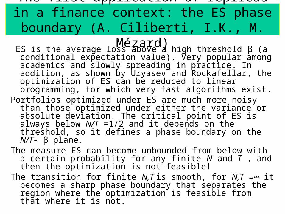
The first application of replicas in a finance context: the ES phase boundary

(A. Ciliberti, I.K., M. Mézard) ES is the average loss above a high threshold β (a

conditional expectation value). Very popular among academics and slowly spreading in practice. In addition, as shown by Uryasev and Rockafellar, the optimization of ES can be reduced to linear programming, for which very fast algorithms exist.

Portfolios optimized under ES are much more noisy than those optimized under either the variance or absolute deviation. The critical point of ES is always below N/T =1/2 and it depends on the threshold, so it defines a phase boundary on the N/T- β plane.

The measure ES can become unbounded from below with a certain probability for any finite N and T , and then the optimization is not feasible!

The transition for finite N,T is smooth, for N,T →∞ it becomes a sharp phase boundary that separates the region where the optimization is feasible from that where it is not.

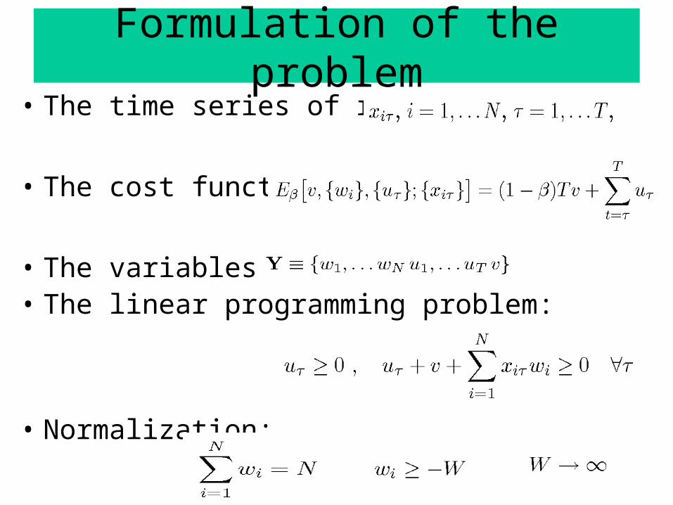
Formulation of the problem• The time series of returns:

• The cost function:

• The variables:• The linear programming problem:

• Normalization:

Associated statistical mechanics problem

• Partition function:

• Free energy:

• The optimal value of the cost function:

The partition function

Lagrange multipliers:

Replicas

• Trivial identity

• We consider n identical replicas:

• The probability distribution of the n-fold replicated system:

• At an appropriate moment we have to analytically continue to real n’s

Averaging over the random samples

where

Replica-symmetric Ansatz

• By symmetry considerations:

• Saddle point condition:

where

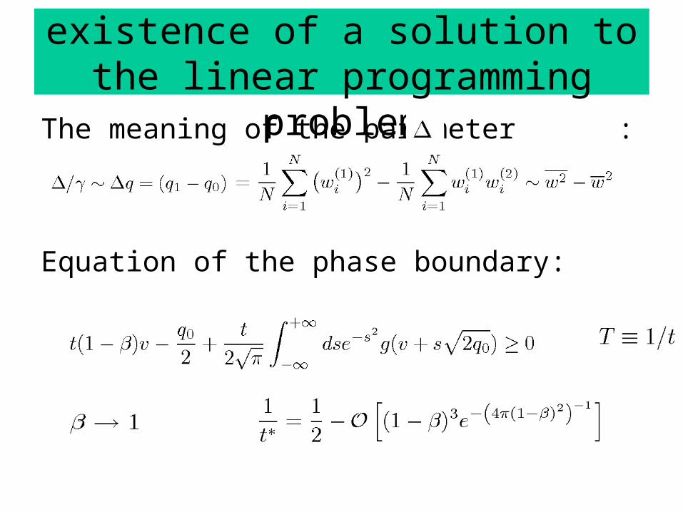
Condition for the existence of a solution to the linear programming problem

The meaning of the parameter :

Equation of the phase boundary:

Portfolio optimization and linear regression

Portfolios:

N

iiip rw

1

11

N

iiw

pwi

Varmin,

j

N

jiiijpp wwCr

1,

VarVar

Linear regression:

.

1

10

N

iii xy

Varmin

1,...,10 , N

21

10

2Var)(

N

iii xyEER

0,Cov,Cov2)( 1

1

N

ijiij

j

yxxxR

0)(2)( 1

10

0

N

ii yExE

R

Equivalence of the two

1

10

N

iii xy

1

1

1

10

1

1

1

1

1

10

1N

iii

N

ii

N

iii

N

ii

N

ii

yxyy

xyyy

Translation

yxr ii yrN

0 p iiw

1

1

1N

iiNw p

Minimizing the residual error for an infinitely large sample

1

10

N

iii xy

Varmin1,...,10 , N

0)( E

*1

*1

*0 ,...,, N

1

1

**0

*N

iii xy ** Var

Minimizing the residual error for a sample of length T

1

10

N

iititt xy

T

ttT 1

01

*1

*1

*0

ˆ,...,ˆ,ˆN

T

ttTN 1

2

,

1min

1,...,10

1

1

**0

* ˆˆˆN

iii xy *** ˆVarˆ

The relative error

1

Var

ˆVarˆ*

*

0

q

Summary

• If we do not have sufficient information we cannot make an intelligent decision, nor can we build a good model – so far this is a triviality

• The important message here is that there is a critical point in both the optimization problem and in the regression problem where the error diverges, and its behaviour is subject to universal scaling laws

• Normally, one is supposed to work in the N<<T limit, i.e. with low dimensional problems and plenty of data.

• Modern portfolio management (e.g. in hedge funds) forces us to consider very large portfolios, but the amount of input information is always limited. So we have N ~ T, or even N>T.

• Complex systems are very high dimensional and irreducible (incompressible), they require a large number of explicatory variables for their faithful representation.

• The dimensionality of the minimal model providing an acceptable representation of a system can be regarded as a measure of the complexity of the system. (Cf. Kolmogorov – Chaitin measure of the complexity of a string. Also Jorge Luis Borges’ map.)

• Therefore, also in the regression problem we have to face the unconventional situation where N~T, or N>T, where the error in the regression coefficients will be large.

• If the number of explicatory variables is very large and they are all of the same order of magnitude, then there is no structure in the system, it is just noise (like a completely random string). So we have to assume that some of the variables have a larger weight than others, but we do not have a natural cutoff beyond which it would be safe to forget about the higher order variables. This leads us to the assumption that the regression coefficients must have a scale free, power law like distribution for complex systems.

• The regression coefficients are proportional to the covariances of the dependent and independent variables. A power law like distribution of the regression coefficients implies the same for the covariances.

• In a physical system this translates into the power law like distribution of the correlations.

• The usual behaviour of correlations in simple systems is not like this: correlations fall off typically exponentially.

• Exceptions: systems at a critical point, or systems with a broken continuous symmetry. Both these are very special cases, however.

• Correlations in a spin glass decay like a power, without any continuous symmetry!

• The power law like behaviour of correlations is a typical behaviour in the spin glass phase.

• A related phenomenon is what is called chaos in spin glasses.

• The long range correlations and the multiplicity of ground states explain the extreme sensitivity of the ground states: the system reacts to any slight external disturbance, but the statistical properties of the new ground state are the same as before: this is a kind of adaptation or learning process.

• Other complex systems? Adaptation, learning, evolution, self-reflectivity cannot be expected to appear in systems with a translationally invariant and all-ferromagnetic coupling. Some of the characteristic features of spin glasses (competition and cooperation, the existence of many metastable equilibria, sensitivity, long range correlations) seem to be necessary minimal properties of any complex system.

• This also means that we will always face the information deficite catastrophe when we try to build a model for a complex system.

• How can we understand that people (in the social sciences, medical sciences, etc.) are getting away with lousy statistics, even with N>T?

• They are projecting external information into their statistical assessments. (I can draw a well-determined straight line across even a single point, if I know that it must be parallel to another line.)

• Humans do not optimize, but use quick and dirty heuristics. This has an evolutionary meaning: if something looks vaguely like a leopard, one jumps, rather than trying to seek the optimal fit to the observed fragments of the picture to a leopard.

• Prior knowledge, the „larger picture”, deliberate or unconscious bias, etc. are essential features of model building.

• When we have a chance to check this prior knowledge millions of times in carefully designed laboratory experiments, this is a well-justified procedure.

• In several applications (macroeconomics, medical sciences, epidemology, etc.) there is no way to perform these laboratory checks, and errors may build up as one uncertain piece of knowledge serves as a prior for another uncertain statistical model. This is how we construct myths, ideologies and social theories.

• It is conceivable that theory building, in the sense of constructing a low dimensional model, for social phenomena will prove to be impossible, and the best we will be able to do is to build a life-size computer model of the system, a kind of gigantic Simcity.

• It remains to be seen what we will mean by understanding under those circumstances.