Lect_3 Two-Dimensional Systems

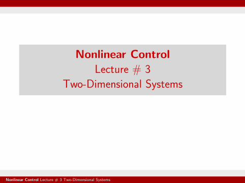
Nonlinear Control

Lecture # 3

Two-Dimensional Systems

Nonlinear Control Lecture # 3 Two-Dimensional Systems

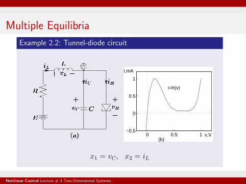
Multiple Equilibria

Example 2.2: Tunnel-diode circuit

1

P

P

�

�

�

�

�

�

�

�

�

P

P

P

P

P

P

P

P

R

��

L

C

v

C

+

�

J

J

J

v

R

�

+

E

s

i

C

i

R

C

C

�

�

C

C

�

�

i

L

v

L

+ �

�

�

X

X

(a)

0 0.5 1−0.5

0

0.5

1

i=h(v)

v,V

i,mA

(b)

x1 = vC , x2 = iL


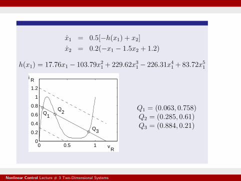
x1 = 0.5[−h(x1) + x2]

x2 = 0.2(−x1 − 1.5x2 + 1.2)

h(x1) = 17.76x1 − 103.79x2

1+ 229.62x3

1− 226.31x4

1+ 83.72x5

1

0 0.5 10

0.2

0.4

0.6

0.8

1

1.2

Q

Q

Q1

2

3

vR

i R

Q1 = (0.063, 0.758)Q2 = (0.285, 0.61)Q3 = (0.884, 0.21)


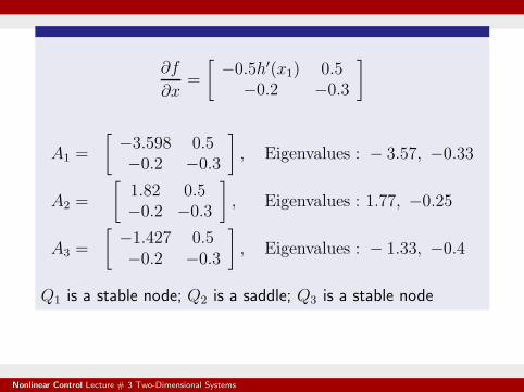
∂f

∂x=

[

−0.5h′(x1) 0.5−0.2 −0.3

]

A1 =

[

−3.598 0.5−0.2 −0.3

]

, Eigenvalues : − 3.57, −0.33

A2 =

[

1.82 0.5−0.2 −0.3

]

, Eigenvalues : 1.77, −0.25

A3 =

[

−1.427 0.5−0.2 −0.3

]

, Eigenvalues : − 1.33, −0.4

Q1 is a stable node; Q2 is a saddle; Q3 is a stable node


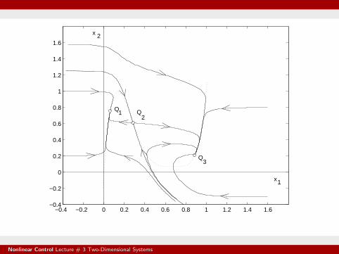
−0.4 −0.2 0 0.2 0.4 0.6 0.8 1 1.2 1.4 1.6−0.4

−0.2

0

0.2

0.4

0.6

0.8

1

1.2

1.4

1.6

x1

x 2

Q2

Q3

Q1


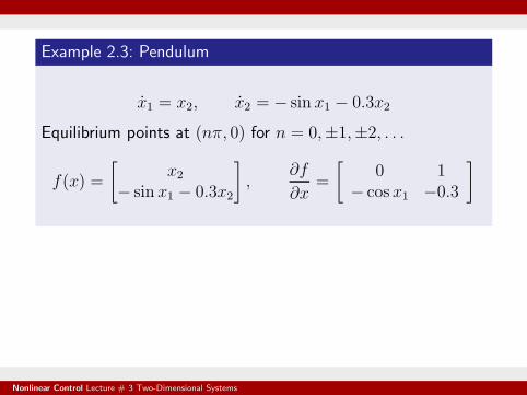
Example 2.3: Pendulum

x1 = x2, x2 = − sin x1 − 0.3x2

Equilibrium points at (nπ, 0) for n = 0,±1,±2, . . .

f(x) =

[

x2

− sin x1 − 0.3x2

]

,∂f

∂x=

[

0 1− cosx1 −0.3

]


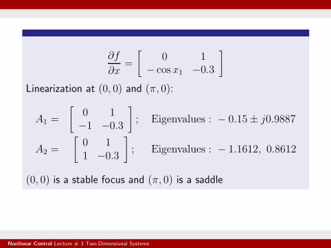
∂f

∂x=

[

0 1− cosx1 −0.3

]

Linearization at (0, 0) and (π, 0):

A1 =

[

0 1−1 −0.3

]

; Eigenvalues : − 0.15± j0.9887

A2 =

[

0 11 −0.3

]

; Eigenvalues : − 1.1612, 0.8612

(0, 0) is a stable focus and (π, 0) is a saddle


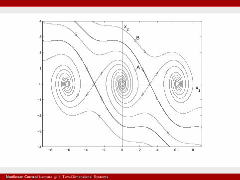
−8 −6 −4 −2 0 2 4 6 8−4

−3

−2

−1

0

1

2

3

4

x2

B

A

x1


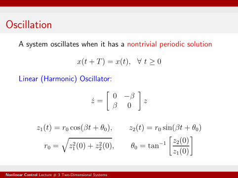
Oscillation

A system oscillates when it has a nontrivial periodic solution

x(t+ T ) = x(t), ∀ t ≥ 0

Linear (Harmonic) Oscillator:

z =

[

0 −β

β 0

]

z

z1(t) = r0 cos(βt+ θ0), z2(t) = r0 sin(βt+ θ0)

r0 =√

z21(0) + z2

2(0), θ0 = tan−1

[

z2(0)

z1(0)

]


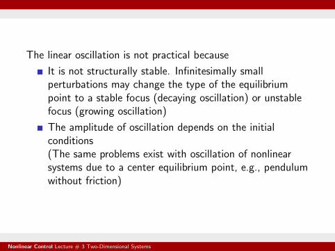
The linear oscillation is not practical because

It is not structurally stable. Infinitesimally smallperturbations may change the type of the equilibriumpoint to a stable focus (decaying oscillation) or unstablefocus (growing oscillation)

The amplitude of oscillation depends on the initialconditions(The same problems exist with oscillation of nonlinearsystems due to a center equilibrium point, e.g., pendulumwithout friction)


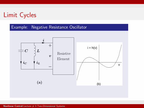
Limit Cycles

Example: Negative Resistance Oscillator

C

iC

✟✠

✟✠

✟✠

✟✠

L

iL

Resistive

Element

i

+

−

v

(a)

❈❈✄✄ ❈❈✄✄

✘✘❳❳

v

(b)

i = h(v)


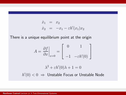
x1 = x2

x2 = −x1 − εh′(x1)x2

There is a unique equilibrium point at the origin

A =∂f

∂x

∣

∣

∣

∣

x=0

=

0 1

−1 −εh′(0)

λ2 + εh′(0)λ+ 1 = 0

h′(0) < 0 ⇒ Unstable Focus or Unstable Node


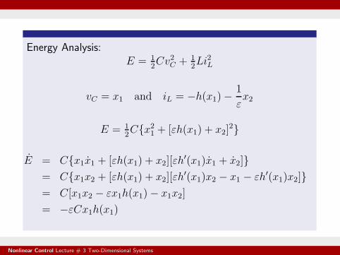
Energy Analysis:E = 1

2Cv2C + 1

2Li2L

vC = x1 and iL = −h(x1)−1

εx2

E = 1

2C{x2

1+ [εh(x1) + x2]

2}

E = C{x1x1 + [εh(x1) + x2][εh′(x1)x1 + x2]}

= C{x1x2 + [εh(x1) + x2][εh′(x1)x2 − x1 − εh′(x1)x2]}

= C[x1x2 − εx1h(x1)− x1x2]

= −εCx1h(x1)


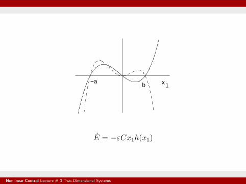
x1−a

b

E = −εCx1h(x1)


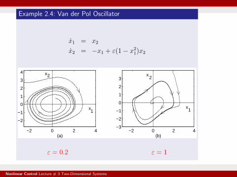
Example 2.4: Van der Pol Oscillator

x1 = x2

x2 = −x1 + ε(1− x2

1)x2

−2 0 2 4−3

−2

−1

0

1

2

3

(b)

x1

x2

−2 0 2 4

−2

−1

0

1

2

3

4

(a)

x1

x2

ε = 0.2 ε = 1


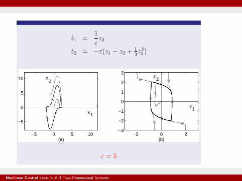
z1 =1

εz2

z2 = −ε(z1 − z2 +1

3z32)

−2 0 2−3

−2

−1

0

1

2

3

(b)

z1

z2

−5 0 5 10

−5

0

5

10

(a)

x1

x2

ε = 5


x1

x2

(a)

x1

x2

(b)

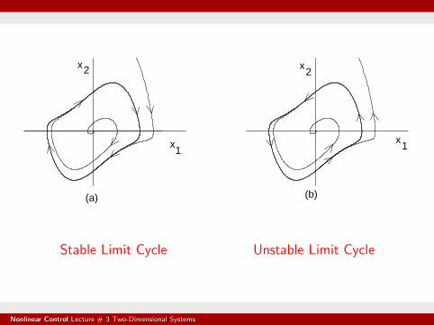
Stable Limit Cycle Unstable Limit Cycle


Documents

Lect_3 Two-Dimensional Systems