Lecture 2 Linear functions and examples - Stanford …ee263.stanford.edu/archive/lin-fcts.pdf · Lecture 2 Linear functions and examples • linear equations and functions • engineering

EE263 Autumn 2008-09 Stephen Boyd

Lecture 2Linear functions and examples

• linear equations and functions

• engineering examples

• interpretations

2–1

Linear equations

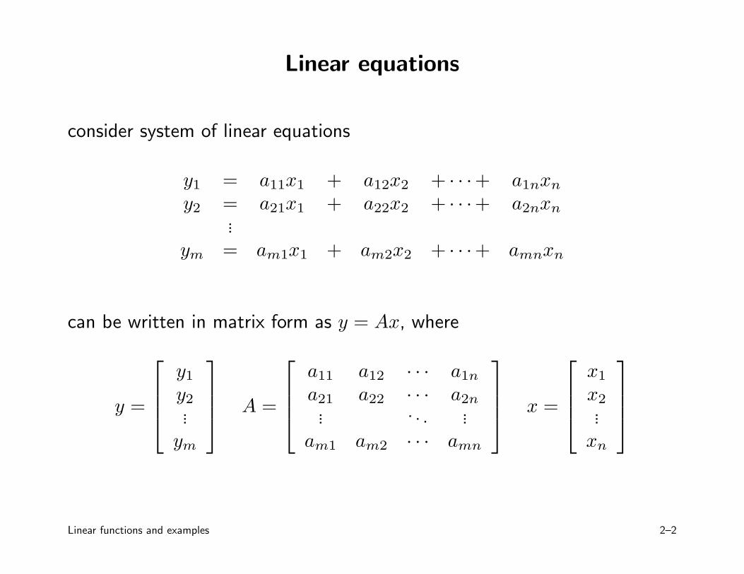
consider system of linear equations

y1 = a11x1 + a12x2 + · · ·+ a1nxn

y2 = a21x1 + a22x2 + · · ·+ a2nxn...

ym = am1x1 + am2x2 + · · ·+ amnxn

can be written in matrix form as y = Ax, where

y =

y1

y2...

ym

A =

a11 a12 · · · a1n

a21 a22 · · · a2n... . . . ...

am1 am2 · · · amn

x =

x1

x2...

xn

Linear functions and examples 2–2

Linear functions

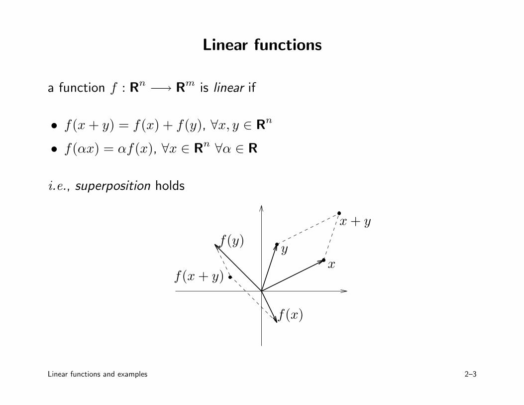
a function f : Rn −→ Rm is linear if

• f(x + y) = f(x) + f(y), ∀x, y ∈ Rn

• f(αx) = αf(x), ∀x ∈ Rn ∀α ∈ R

i.e., superposition holds

xy

x + y

f(x)

f(y)

f(x + y)


Matrix multiplication function

• consider function f : Rn → Rm given by f(x) = Ax, where A ∈ Rm×n

• matrix multiplication function f is linear

• converse is true: any linear function f : Rn → Rm can be written asf(x) = Ax for some A ∈ Rm×n

• representation via matrix multiplication is unique: for any linearfunction f there is only one matrix A for which f(x) = Ax for all x

• y = Ax is a concrete representation of a generic linear function


Interpretations of y = Ax

• y is measurement or observation; x is unknown to be determined

• x is ‘input’ or ‘action’; y is ‘output’ or ‘result’

• y = Ax defines a function or transformation that maps x ∈ Rn intoy ∈ Rm


Interpretation of aij

yi =

n∑

j=1

aijxj

aij is gain factor from jth input (xj) to ith output (yi)

thus, e.g.,

• ith row of A concerns ith output

• jth column of A concerns jth input

• a27 = 0 means 2nd output (y2) doesn’t depend on 7th input (x7)

• |a31| ≫ |a3j| for j 6= 1 means y3 depends mainly on x1


• |a52| ≫ |ai2| for i 6= 5 means x2 affects mainly y5

• A is lower triangular, i.e., aij = 0 for i < j, means yi only depends onx1, . . . , xi

• A is diagonal, i.e., aij = 0 for i 6= j, means ith output depends only onith input

more generally, sparsity pattern of A, i.e., list of zero/nonzero entries ofA, shows which xj affect which yi


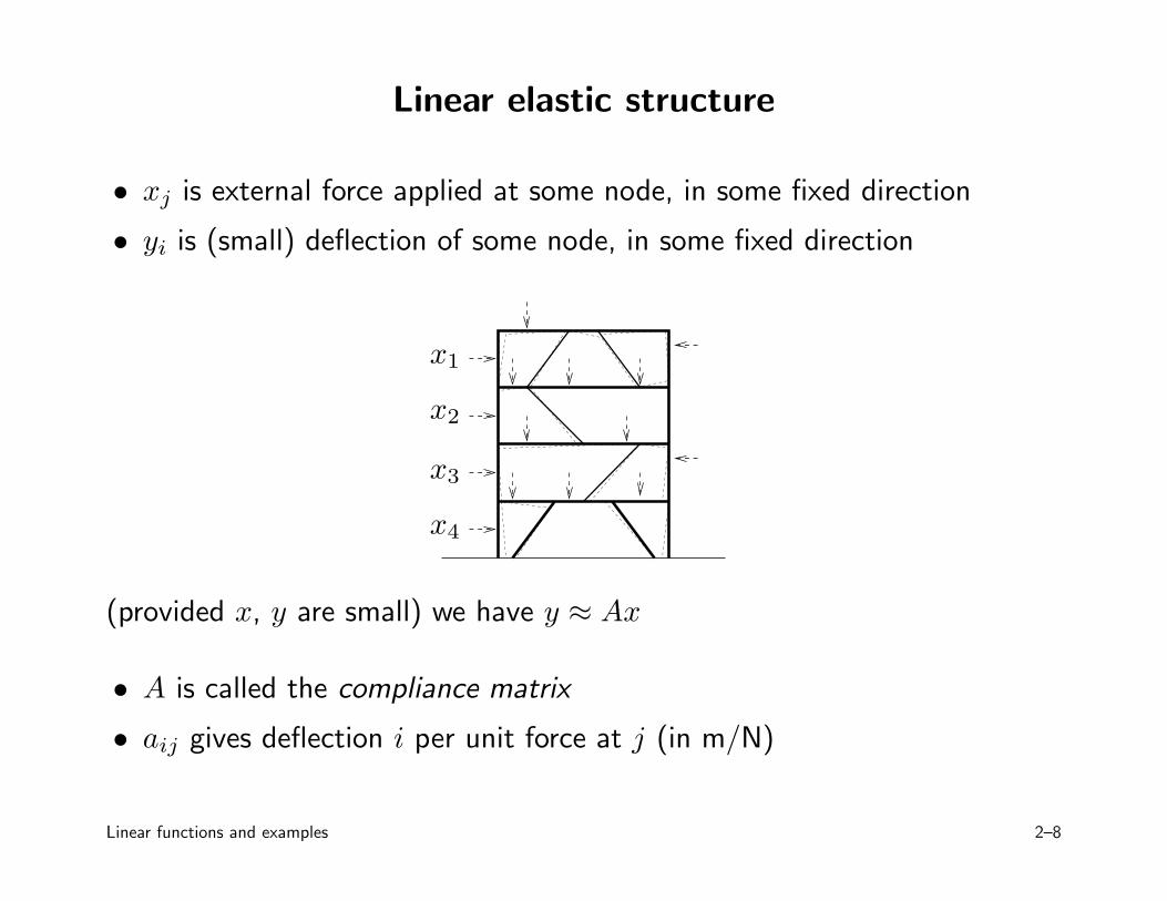
Linear elastic structure

• xj is external force applied at some node, in some fixed direction

• yi is (small) deflection of some node, in some fixed direction

x1

x2

x3

x4

(provided x, y are small) we have y ≈ Ax

• A is called the compliance matrix

• aij gives deflection i per unit force at j (in m/N)


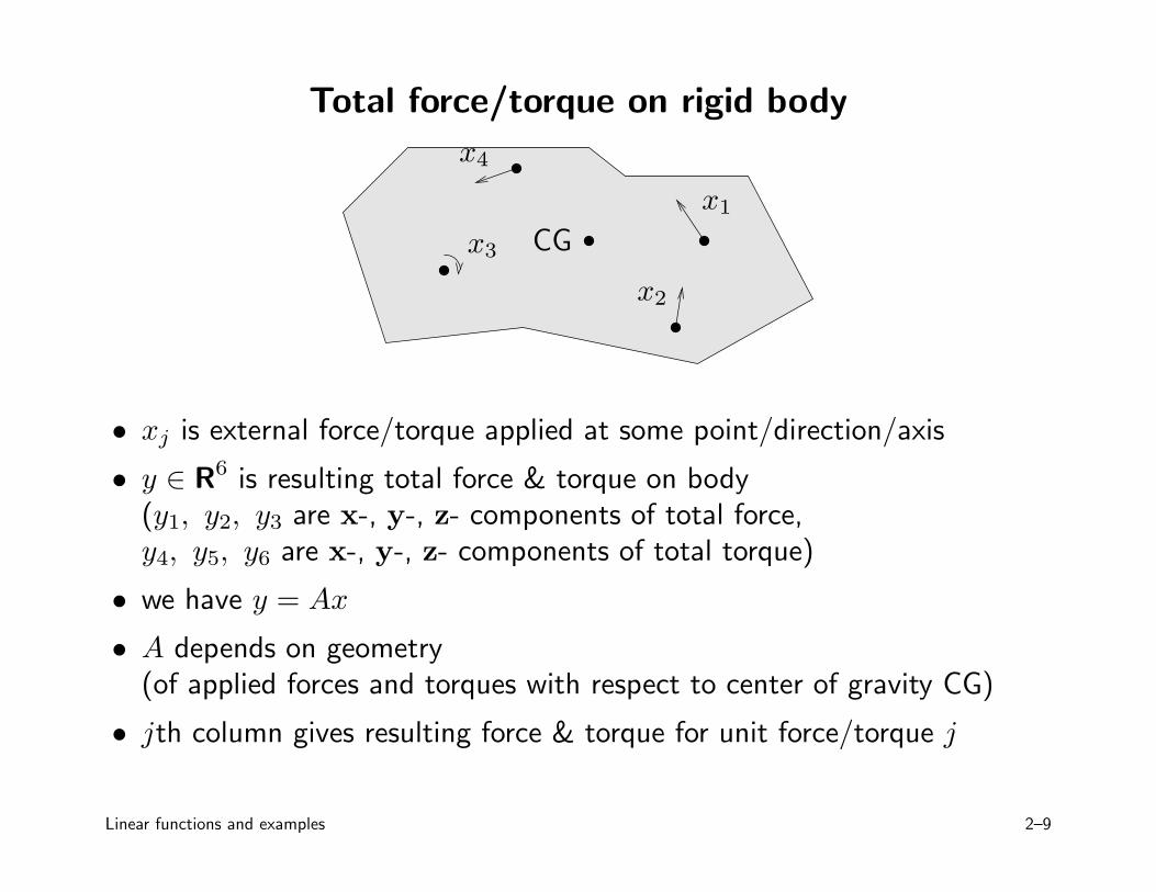
Total force/torque on rigid body

x1

x2

x3

x4

CG

• xj is external force/torque applied at some point/direction/axis

• y ∈ R6 is resulting total force & torque on body(y1, y2, y3 are x-, y-, z- components of total force,y4, y5, y6 are x-, y-, z- components of total torque)

• we have y = Ax

• A depends on geometry(of applied forces and torques with respect to center of gravity CG)

• jth column gives resulting force & torque for unit force/torque j


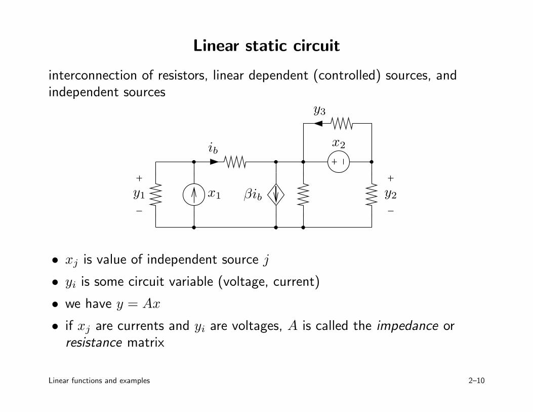
Linear static circuit

interconnection of resistors, linear dependent (controlled) sources, andindependent sources

x1

x2

y1 y2

y3

ib

βib

• xj is value of independent source j

• yi is some circuit variable (voltage, current)

• we have y = Ax

• if xj are currents and yi are voltages, A is called the impedance orresistance matrix


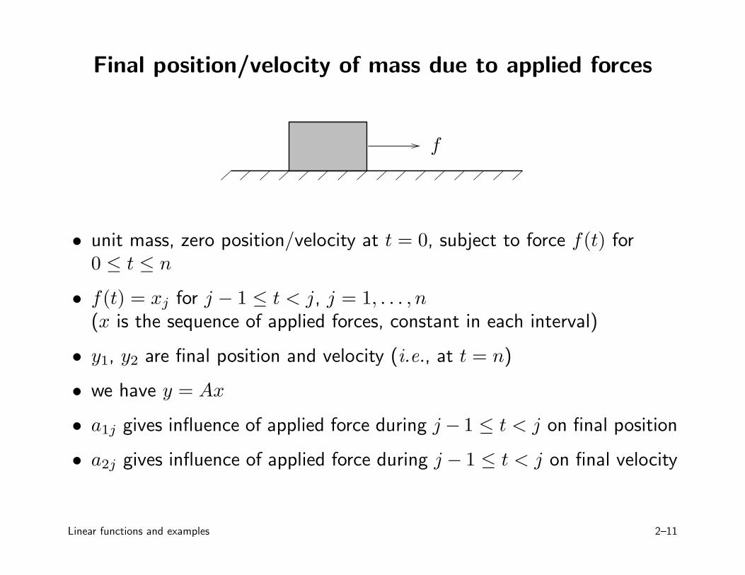
Final position/velocity of mass due to applied forces

f

• unit mass, zero position/velocity at t = 0, subject to force f(t) for0 ≤ t ≤ n

• f(t) = xj for j − 1 ≤ t < j, j = 1, . . . , n

(x is the sequence of applied forces, constant in each interval)

• y1, y2 are final position and velocity (i.e., at t = n)

• we have y = Ax

• a1j gives influence of applied force during j − 1 ≤ t < j on final position

• a2j gives influence of applied force during j − 1 ≤ t < j on final velocity


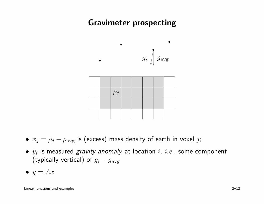
Gravimeter prospecting

ρj

gi gavg

• xj = ρj − ρavg is (excess) mass density of earth in voxel j;

• yi is measured gravity anomaly at location i, i.e., some component(typically vertical) of gi − gavg

• y = Ax


• A comes from physics and geometry

• jth column of A shows sensor readings caused by unit density anomalyat voxel j

• ith row of A shows sensitivity pattern of sensor i


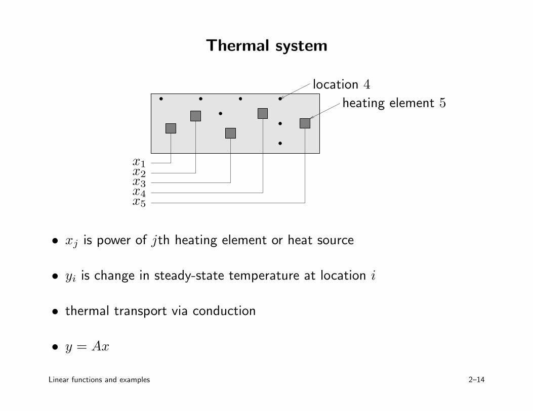
Thermal system

x1x2x3x4x5

location 4

heating element 5

• xj is power of jth heating element or heat source

• yi is change in steady-state temperature at location i

• thermal transport via conduction

• y = Ax


• aij gives influence of heater j at location i (in ◦C/W)

• jth column of A gives pattern of steady-state temperature rise due to1W at heater j

• ith row shows how heaters affect location i


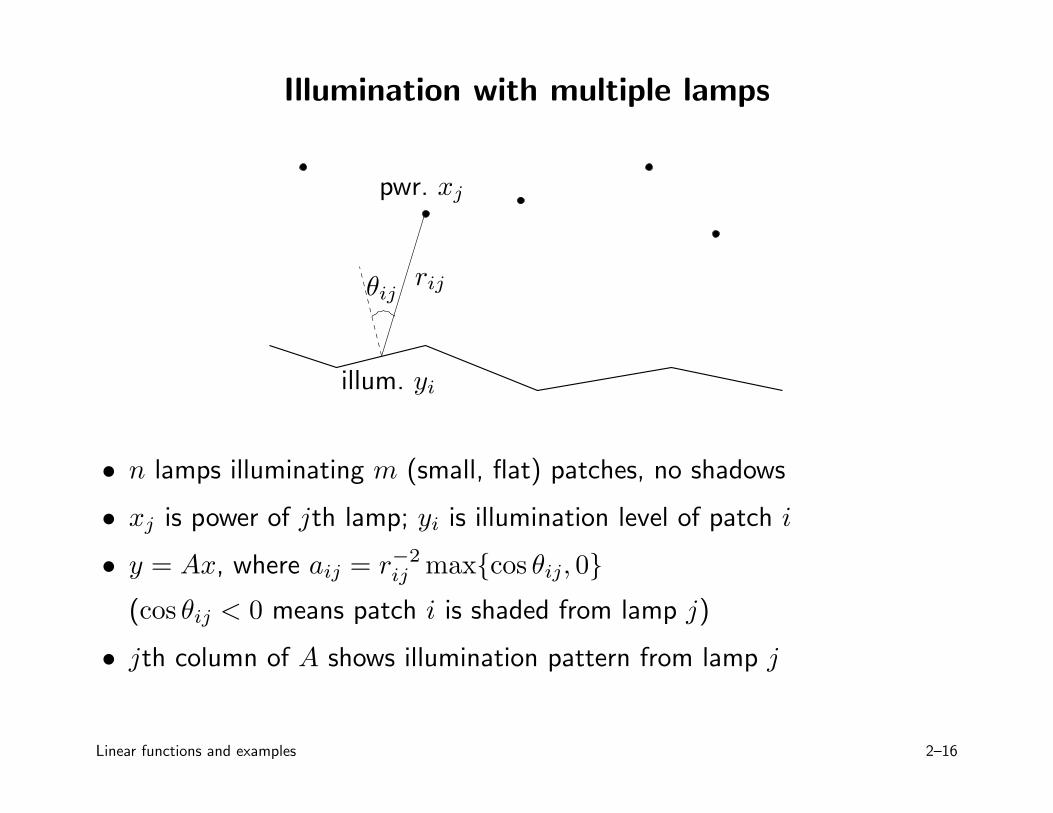
Illumination with multiple lamps

pwr. xj

illum. yi

rijθij

• n lamps illuminating m (small, flat) patches, no shadows

• xj is power of jth lamp; yi is illumination level of patch i

• y = Ax, where aij = r−2ij max{cos θij, 0}

(cos θij < 0 means patch i is shaded from lamp j)

• jth column of A shows illumination pattern from lamp j


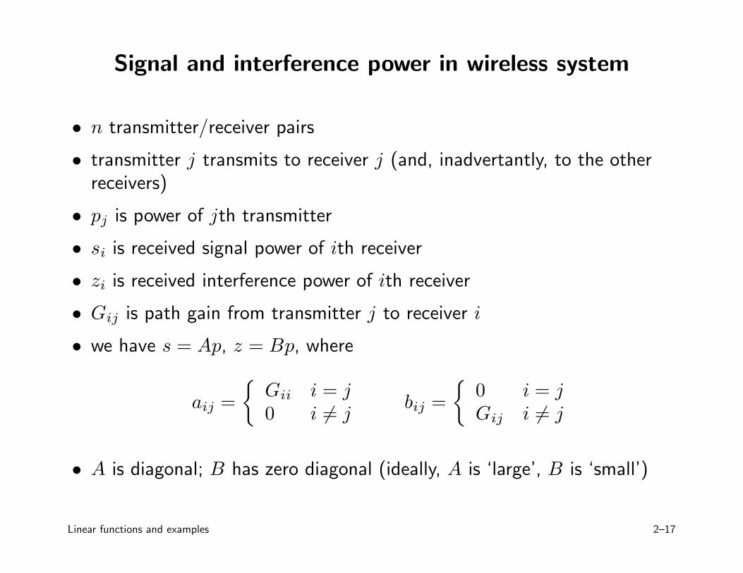
Signal and interference power in wireless system

• n transmitter/receiver pairs

• transmitter j transmits to receiver j (and, inadvertantly, to the otherreceivers)

• pj is power of jth transmitter

• si is received signal power of ith receiver

• zi is received interference power of ith receiver

• Gij is path gain from transmitter j to receiver i

• we have s = Ap, z = Bp, where

aij =

{

Gii i = j

0 i 6= jbij =

{

0 i = j

Gij i 6= j

• A is diagonal; B has zero diagonal (ideally, A is ‘large’, B is ‘small’)


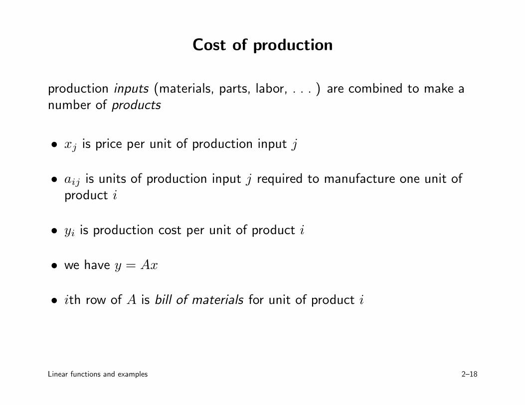
Cost of production

production inputs (materials, parts, labor, . . . ) are combined to make anumber of products

• xj is price per unit of production input j

• aij is units of production input j required to manufacture one unit ofproduct i

• yi is production cost per unit of product i

• we have y = Ax

• ith row of A is bill of materials for unit of product i


production inputs needed

• qi is quantity of product i to be produced

• rj is total quantity of production input j needed

• we have r = ATq

total production cost is

rTx = (ATq)Tx = qTAx


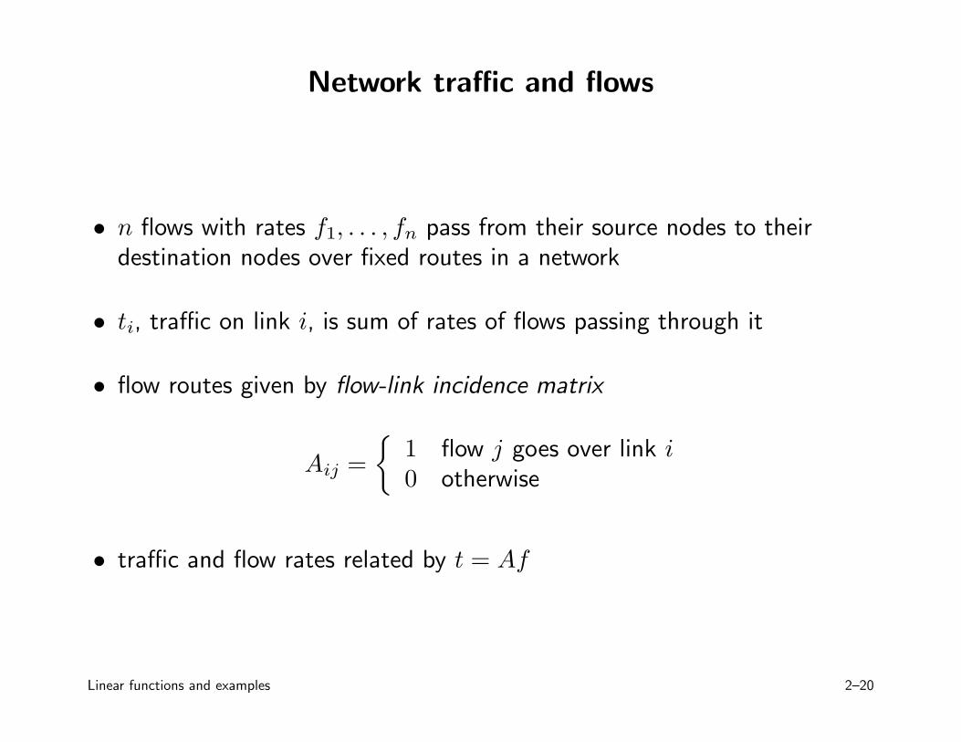
Network traffic and flows

• n flows with rates f1, . . . , fn pass from their source nodes to theirdestination nodes over fixed routes in a network

• ti, traffic on link i, is sum of rates of flows passing through it

• flow routes given by flow-link incidence matrix

Aij =

{

1 flow j goes over link i

0 otherwise

• traffic and flow rates related by t = Af


link delays and flow latency

• let d1, . . . , dm be link delays, and l1, . . . , ln be latency (total traveltime) of flows

• l = ATd

• fT l = fTATd = (Af)Td = tTd, total # of packets in network


Linearization

• if f : Rn → Rm is differentiable at x0 ∈ Rn, then

x near x0 =⇒ f(x) very near f(x0) + Df(x0)(x − x0)

where

Df(x0)ij =∂fi

∂xj

∣

∣

∣

∣

x0

is derivative (Jacobian) matrix

• with y = f(x), y0 = f(x0), define input deviation δx := x − x0, output

deviation δy := y − y0

• then we have δy ≈ Df(x0)δx

• when deviations are small, they are (approximately) related by a linearfunction


Navigation by range measurement

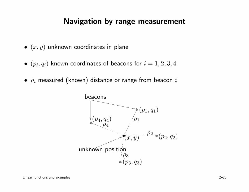
• (x, y) unknown coordinates in plane

• (pi, qi) known coordinates of beacons for i = 1, 2, 3, 4

• ρi measured (known) distance or range from beacon i

(x, y)

(p1, q1)

(p2, q2)

(p3, q3)

(p4, q4) ρ1

ρ2

ρ3

ρ4

beacons

unknown position


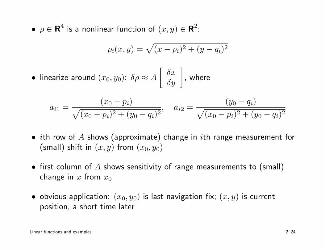
• ρ ∈ R4 is a nonlinear function of (x, y) ∈ R2:

ρi(x, y) =√

(x − pi)2 + (y − qi)2

• linearize around (x0, y0): δρ ≈ A

[

δx

δy

]

, where

ai1 =(x0 − pi)

√

(x0 − pi)2 + (y0 − qi)2, ai2 =

(y0 − qi)√

(x0 − pi)2 + (y0 − qi)2

• ith row of A shows (approximate) change in ith range measurement for(small) shift in (x, y) from (x0, y0)

• first column of A shows sensitivity of range measurements to (small)change in x from x0

• obvious application: (x0, y0) is last navigation fix; (x, y) is currentposition, a short time later


Broad categories of applications

linear model or function y = Ax

some broad categories of applications:

• estimation or inversion

• control or design

• mapping or transformation

(this list is not exclusive; can have combinations . . . )


Estimation or inversion

y = Ax

• yi is ith measurement or sensor reading (which we know)

• xj is jth parameter to be estimated or determined

• aij is sensitivity of ith sensor to jth parameter

sample problems:

• find x, given y

• find all x’s that result in y (i.e., all x’s consistent with measurements)

• if there is no x such that y = Ax, find x s.t. y ≈ Ax (i.e., if the sensorreadings are inconsistent, find x which is almost consistent)


Control or design

y = Ax

• x is vector of design parameters or inputs (which we can choose)

• y is vector of results, or outcomes

• A describes how input choices affect results

sample problems:

• find x so that y = ydes

• find all x’s that result in y = ydes (i.e., find all designs that meetspecifications)

• among x’s that satisfy y = ydes, find a small one (i.e., find a small orefficient x that meets specifications)


Mapping or transformation

• x is mapped or transformed to y by linear function y = Ax

sample problems:

• determine if there is an x that maps to a given y

• (if possible) find an x that maps to y

• find all x’s that map to a given y

• if there is only one x that maps to y, find it (i.e., decode or undo themapping)


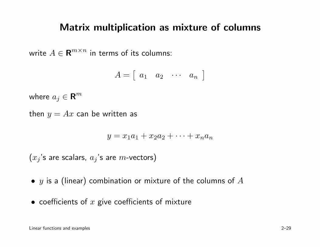
Matrix multiplication as mixture of columns

write A ∈ Rm×n in terms of its columns:

A =[

a1 a2 · · · an

]

where aj ∈ Rm

then y = Ax can be written as

y = x1a1 + x2a2 + · · · + xnan

(xj’s are scalars, aj’s are m-vectors)

• y is a (linear) combination or mixture of the columns of A

• coefficients of x give coefficients of mixture


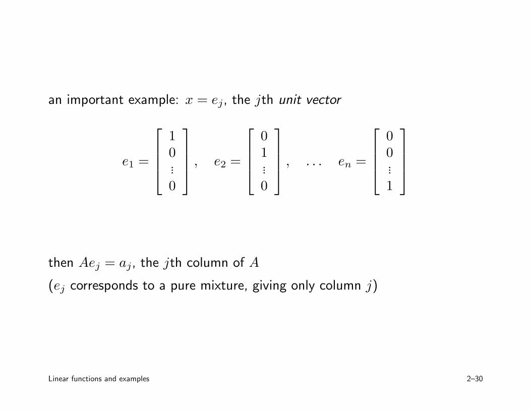
an important example: x = ej, the jth unit vector

e1 =

10...0

, e2 =

01...0

, . . . en =

00...1

then Aej = aj, the jth column of A

(ej corresponds to a pure mixture, giving only column j)


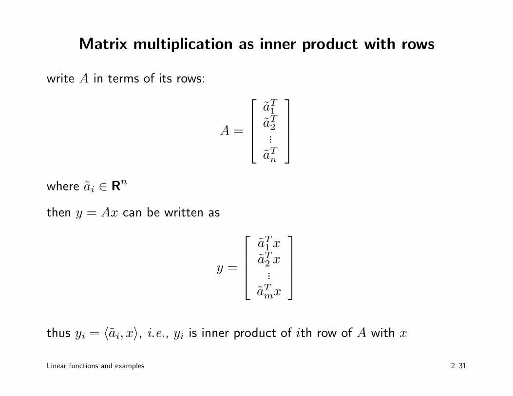
Matrix multiplication as inner product with rows

write A in terms of its rows:

A =

aT1

aT2...

aTn

where ai ∈ Rn

then y = Ax can be written as

y =

aT1 x

aT2 x...

aTmx

thus yi = 〈ai, x〉, i.e., yi is inner product of ith row of A with x


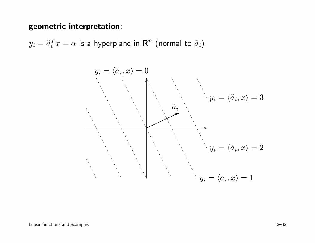
geometric interpretation:

yi = aTi x = α is a hyperplane in Rn (normal to ai)

ai

yi = 〈ai, x〉 = 3

yi = 〈ai, x〉 = 2

yi = 〈ai, x〉 = 1

yi = 〈ai, x〉 = 0


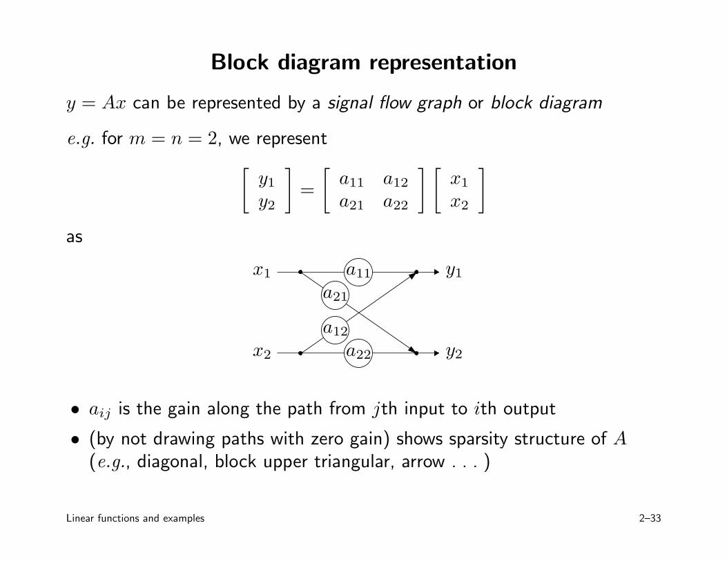
Block diagram representation

y = Ax can be represented by a signal flow graph or block diagram

e.g. for m = n = 2, we represent

[

y1

y2

]

=

[

a11 a12

a21 a22

] [

x1

x2

]

as

x1

x2

y1

y2

a11

a21

a12

a22

• aij is the gain along the path from jth input to ith output

• (by not drawing paths with zero gain) shows sparsity structure of A

(e.g., diagonal, block upper triangular, arrow . . . )


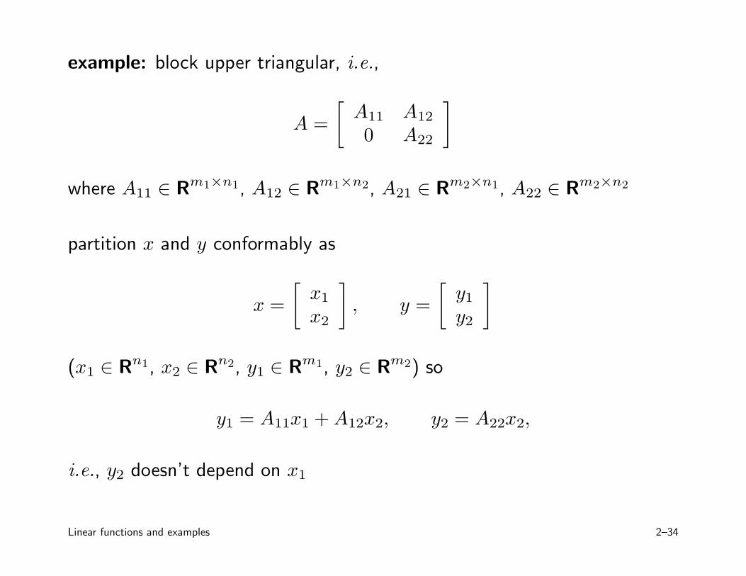
example: block upper triangular, i.e.,

A =

[

A11 A12

0 A22

]

where A11 ∈ Rm1×n1, A12 ∈ Rm1×n2, A21 ∈ Rm2×n1, A22 ∈ Rm2×n2

partition x and y conformably as

x =

[

x1

x2

]

, y =

[

y1

y2

]

(x1 ∈ Rn1, x2 ∈ Rn2, y1 ∈ Rm1, y2 ∈ Rm2) so

y1 = A11x1 + A12x2, y2 = A22x2,

i.e., y2 doesn’t depend on x1


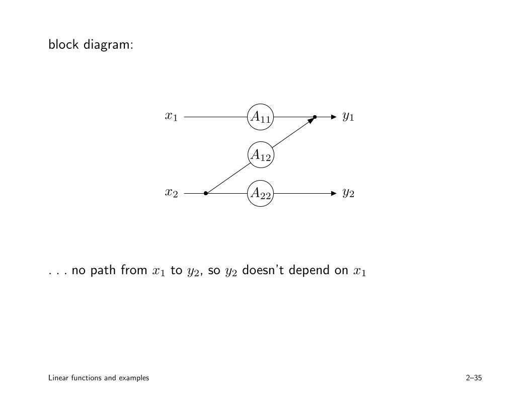
block diagram:

x1

x2

y1

y2

A11

A12

A22

. . . no path from x1 to y2, so y2 doesn’t depend on x1


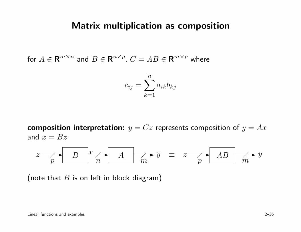
Matrix multiplication as composition

for A ∈ Rm×n and B ∈ Rn×p, C = AB ∈ Rm×p where

cij =

n∑

k=1

aikbkj

composition interpretation: y = Cz represents composition of y = Ax

and x = Bz

mmn ppzz y yx AB AB≡

(note that B is on left in block diagram)


Column and row interpretations

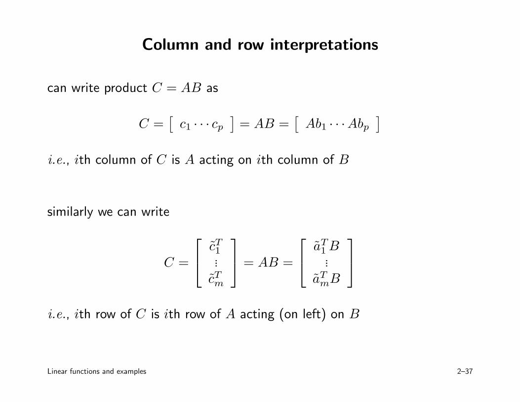
can write product C = AB as

C =[

c1 · · · cp

]

= AB =[

Ab1 · · ·Abp

]

i.e., ith column of C is A acting on ith column of B

similarly we can write

C =

cT1...

cTm

= AB =

aT1 B...

aTmB

i.e., ith row of C is ith row of A acting (on left) on B


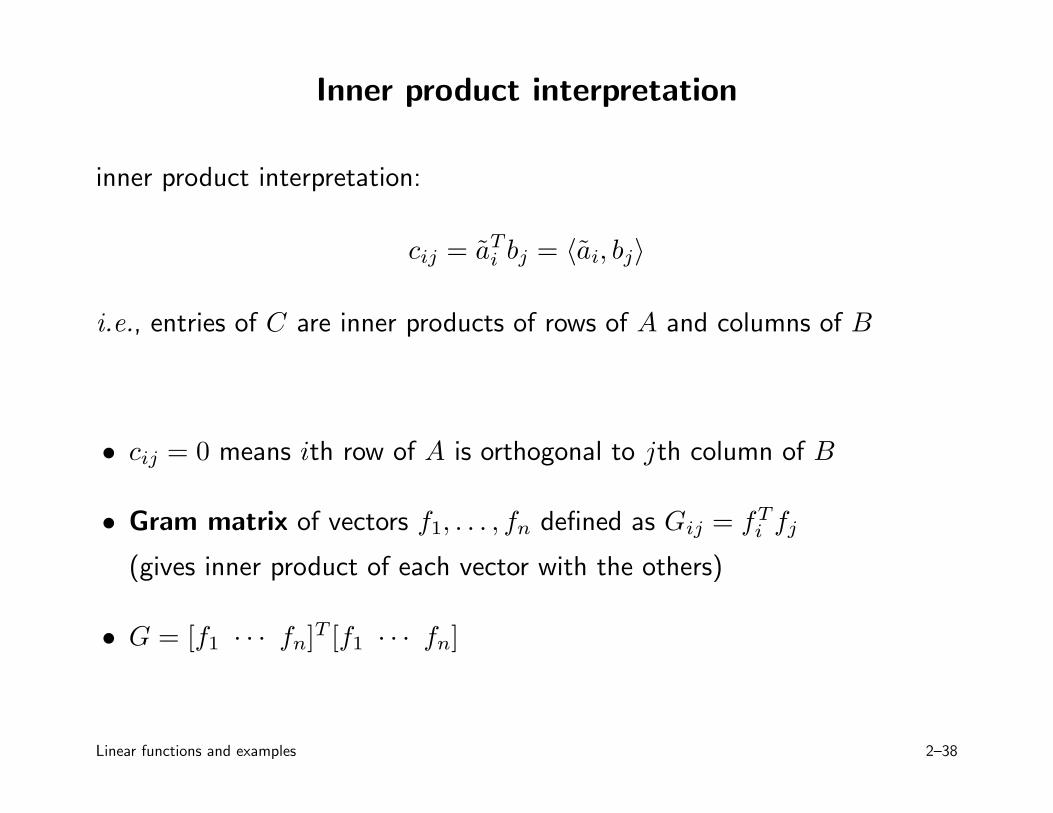
Inner product interpretation

inner product interpretation:

cij = aTi bj = 〈ai, bj〉

i.e., entries of C are inner products of rows of A and columns of B

• cij = 0 means ith row of A is orthogonal to jth column of B

• Gram matrix of vectors f1, . . . , fn defined as Gij = fTi fj

(gives inner product of each vector with the others)

• G = [f1 · · · fn]T [f1 · · · fn]


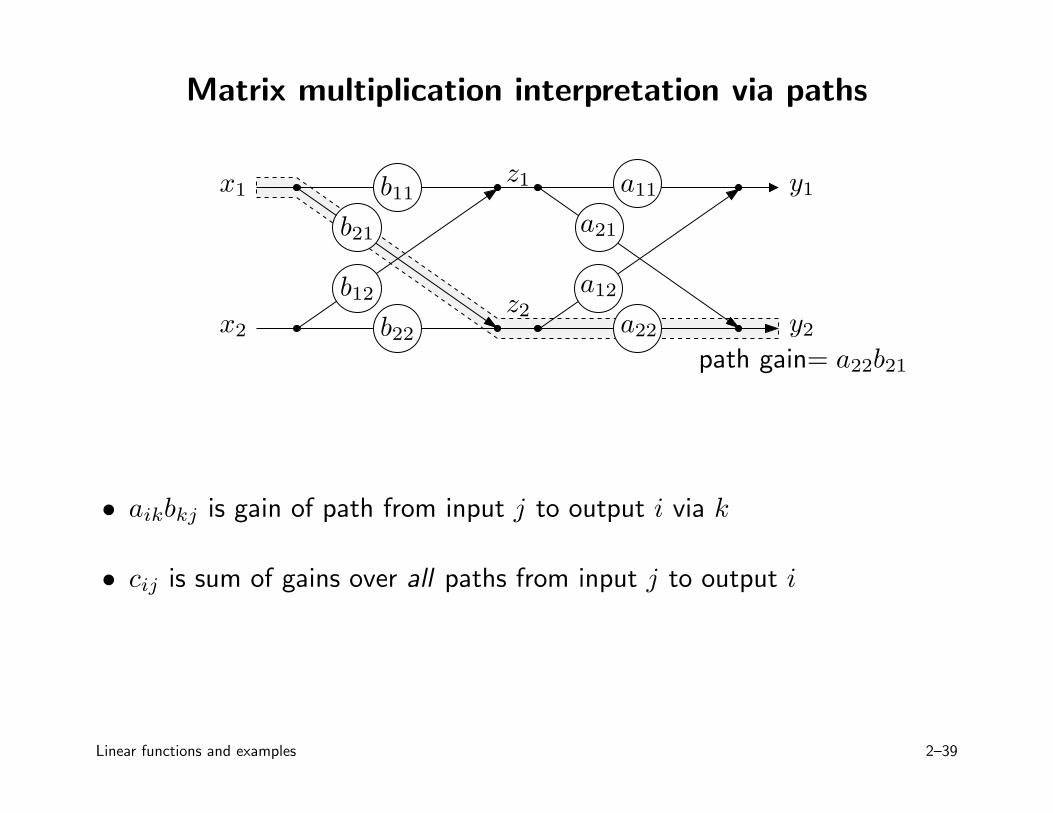
Matrix multiplication interpretation via paths

a11

a21

a12

a22

b11

b21

b12

b22

x1

x2

y1

y2

z1

z2

path gain= a22b21

• aikbkj is gain of path from input j to output i via k

• cij is sum of gains over all paths from input j to output i


Documents

Lecture 2 Linear functions and examples - Stanford …ee263.stanford.edu/archive/lin-fcts.pdf · Lecture 2 Linear functions and examples • linear equations and functions • engineering