Lecture #9 of 18 - UCI Department of Chemistryardo/echem/UCI-CHEM248-2017W_lecture… · use it to measure D! 649 … but what are the problems with this approach? … solution: Integrate

623

Lecture #9 of 18

624

Q: What’s in this set of lectures?

A: B&F Chapters 4 & 5 main concepts:

● Section 4.4.2: Fick’s Second Law of Diffusion

● Section 5.1: Overview of step experiments

● Section 5.2: Potential step under diffusion controlled

● Section 5.3 & 5.9: Ultramicroelectrodes

● Sections 5.7 – 5.8: Chronoamperometry/Chronocoulometry

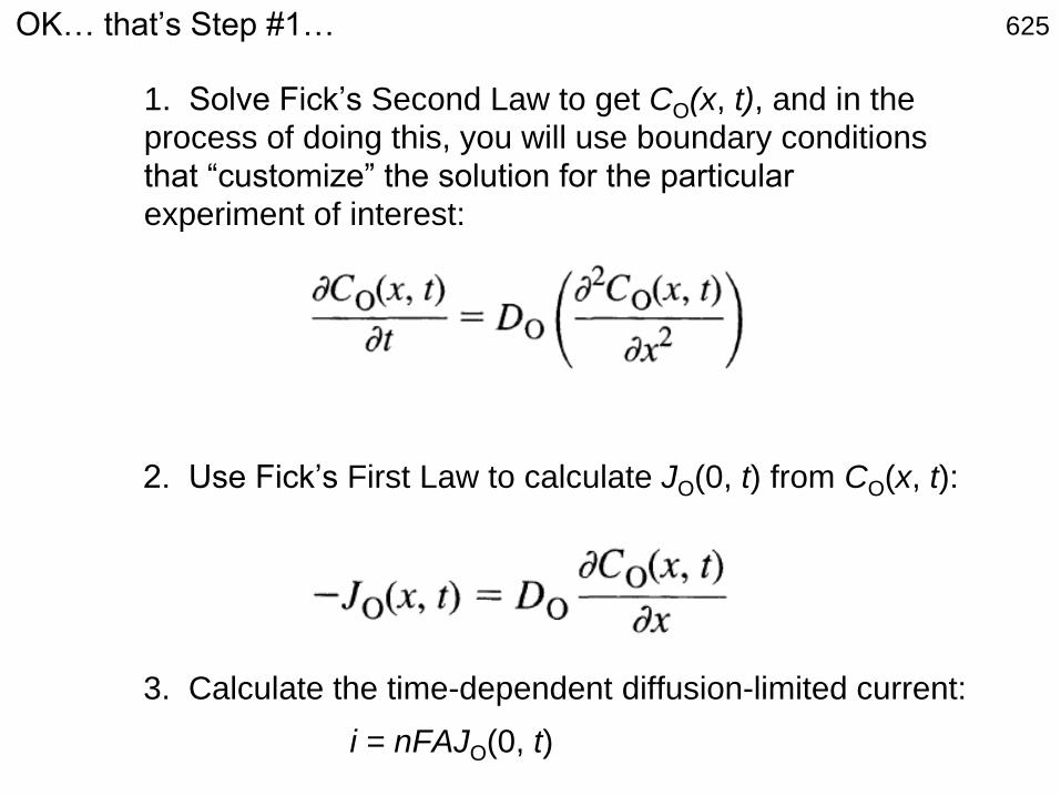
OK… that’s Step #1… 625

1. Solve Fick’s Second Law to get CO(x, t), and in the

process of doing this, you will use boundary conditions

that “customize” the solution for the particular

experiment of interest:

3. Calculate the time-dependent diffusion-limited current:

i = nFAJO(0, t)

2. Use Fick’s First Law to calculate JO(0, t) from CO(x, t):

626now our solution is fully constrained… and we need “t” back!!

inverse L.T. using Table A.1.1 in B&F

=

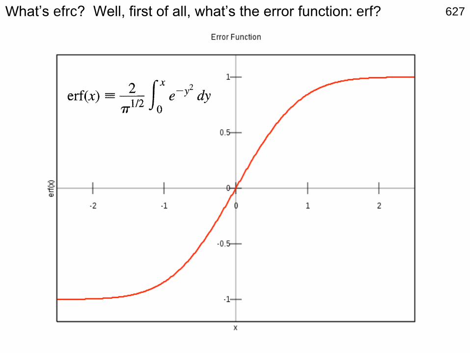
627What’s efrc? Well, first of all, what’s the error function: erf?

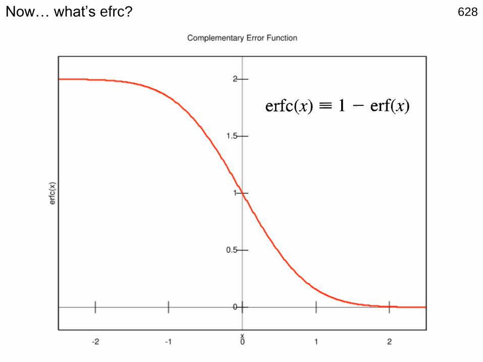
628Now… what’s efrc?

629Now… what’s efrc?

Gaussian distribution,

with mean = 0 and std.

dev. = 1/sqrt(2)

630

… well, for large x, erfc = 0 (erf = 1) and so C(x, t) = C* … Check!

… and for x = 0, erfc = 1 (erf = 0) and so C(x, t) = 0 … Check!

… Let’s plot it!

Does this make sense?

631

C* = 1 x 10-6 M

D = 1 x 10-5 cm2 s-1

t = 1s

0.1s0.01s0.0001s

Hey, these look completely reasonable!

632

root mean square

(rms) displacement

(standard deviation) Δ = 2𝑑 𝐷𝑡, where d is the dimension

D Δ*=

1D

2D

3D

*the rms displacement

plane

wire, line, tube

point, sphere, disk

a characteristic

"diffusion length"

2𝐷𝑡

4𝐷𝑡

6𝐷𝑡

Δ = 2𝑑 𝐷𝑡 =cm2

ss = cm

How large is the diffusion layer? … Recall…

633

4 µm

14 µm 40 µm

t = 1s

0.1s

Hey, these look completely reasonable!

0.01s0.0001s

… use the geometric area for calculations

C* = 1 x 10-6 M

D = 1 x 10-5 cm2 s-1

2𝐷𝑡 =

OK… that’s Step #1… 634

1. Solve Fick’s Second Law to get CO(x, t), and in the



experiment of interest:


i = nFAJO(0, t)

2. Use Fick’s First Law to calculate JO(0, t) from CO(x, t):

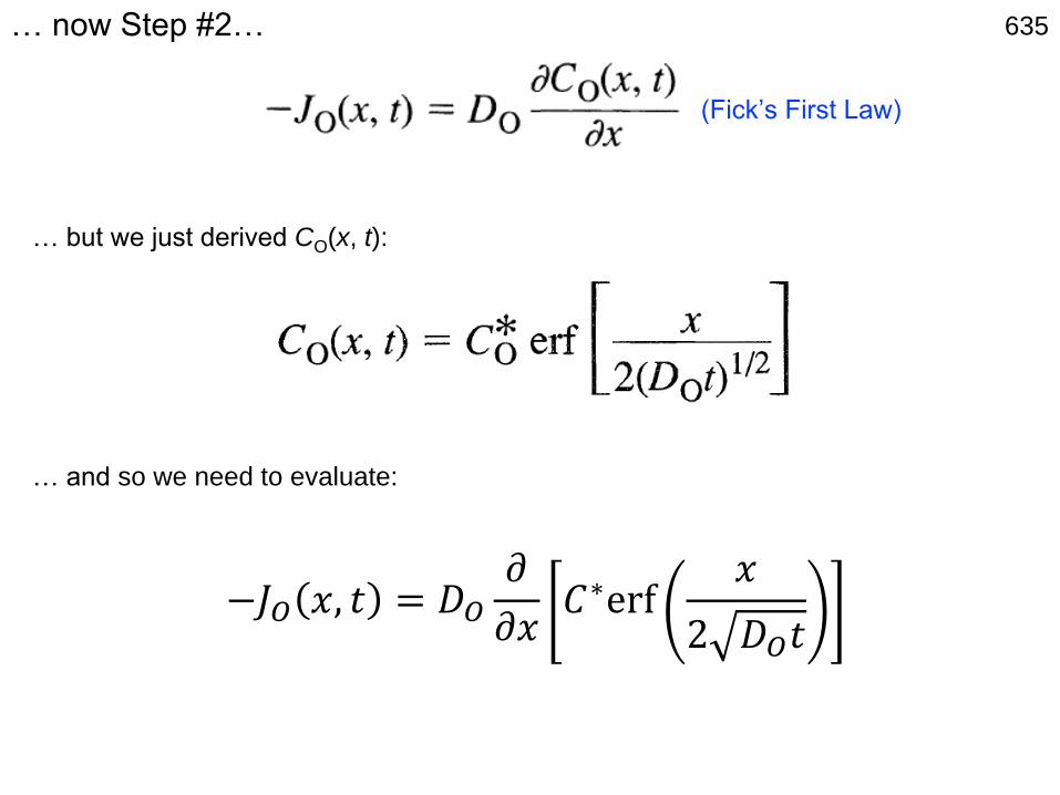
635

… but we just derived CO(x, t):

… now Step #2…

(Fick’s First Law)

… and so we need to evaluate:

−𝐽𝑂 𝑥, 𝑡 = 𝐷𝑂𝜕

𝜕𝑥𝐶∗erf

𝑥

2 𝐷𝑂𝑡

636… now Step #2…

… we use the Liebnitz Rule, to get for d/dx(erf(x)):

see B&F,pg. 780,for details


𝜕𝑥𝐶∗erf

𝑥

2 𝐷𝑡

637… now Step #2…



… and using this in conjunction with the chain rule, we get:


𝜕𝑥𝐶∗erf

𝑥

2 𝐷𝑡

−𝐽𝑂 𝑥, 𝑡 = 𝐷𝑂𝐶∗

1

2 𝐷𝑂𝑡

2

𝜋exp

−𝑥2

4𝐷𝑂𝑡

638


… now Step #2…


… and using this in conjunction with the chain rule, we get:

… and when x = 0, we have what we wanted…


𝜕𝑥𝐶∗erf

𝑥

2 𝐷𝑡

−𝐽𝑂 0, 𝑡 = 𝐶∗𝐷𝑂𝜋𝑡

−𝐽𝑂 𝑥, 𝑡 = 𝐷𝑂𝐶∗

1

2 𝐷𝑂𝑡

2

𝜋exp

−𝑥2

4𝐷𝑂𝑡

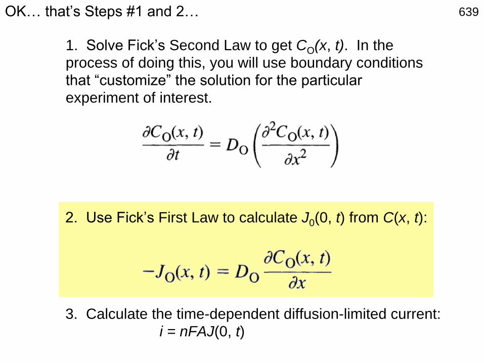
639

1. Solve Fick’s Second Law to get CO(x, t). In the



experiment of interest.


i = nFAJ(0, t)

2. Use Fick’s First Law to calculate J0(0, t) from C(x, t):

OK… that’s Steps #1 and 2…

640… and finally, Step #3 using Step #2…


the Cottrell Equation

… and with i = nFAJ(0, t)…

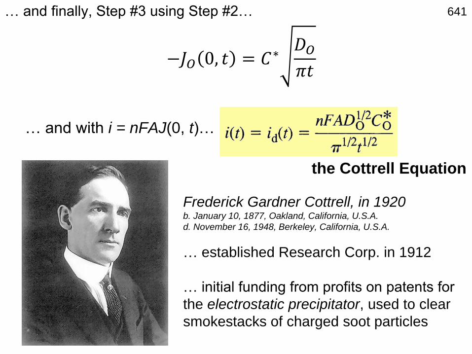
641… and finally, Step #3 using Step #2…

the Cottrell Equation

Frederick Gardner Cottrell, in 1920b. January 10, 1877, Oakland, California, U.S.A.

d. November 16, 1948, Berkeley, California, U.S.A.

… established Research Corp. in 1912

… initial funding from profits on patents for

the electrostatic precipitator, used to clear

smokestacks of charged soot particles

… and with i = nFAJ(0, t)…


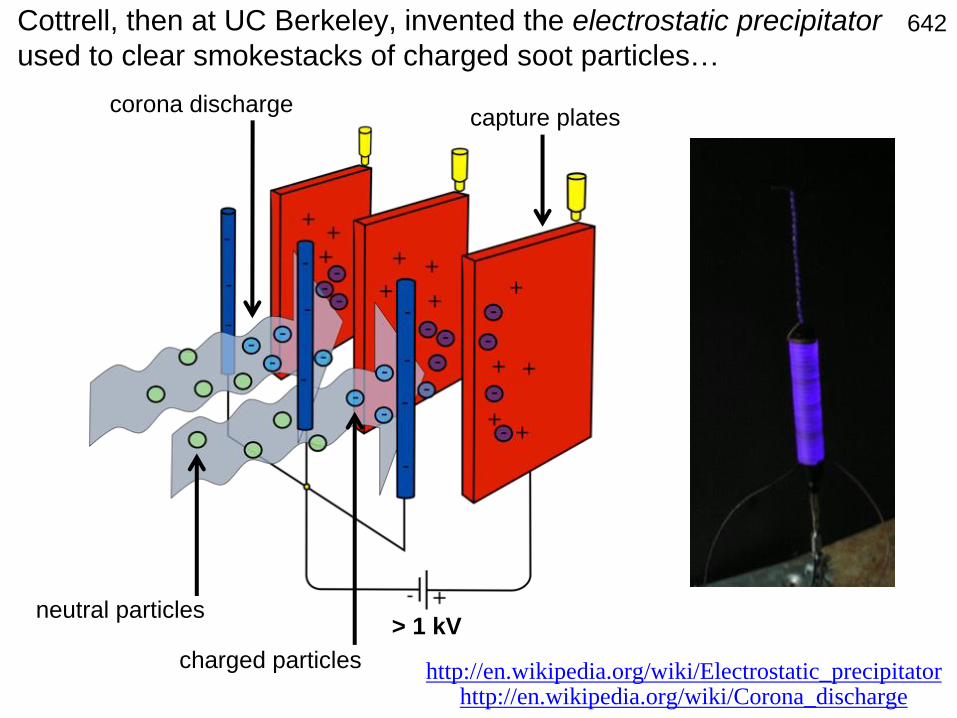
642

http://en.wikipedia.org/wiki/Electrostatic_precipitatorhttp://en.wikipedia.org/wiki/Corona_discharge

> 1 kVneutral particles

corona dischargecapture plates

charged particles

Cottrell, then at UC Berkeley, invented the electrostatic precipitator

used to clear smokestacks of charged soot particles…

http://en.wikipedia.org/wiki/Electrostatic_precipitator

643

644

D = 1.5 x 10-6 cm2 s-1

D = 1 x 10-5 cm2 s-1

… OK, so what does it predict?

the Cottrell

Equation

645

D = 1.5 x 10-6 cm2 s-1

D = 1 x 10-5 cm2 s-1


the Cottrell

Equation

646… OK, so what does it predict?

the Cottrell

Equation

slope =

nFAπ -1/2D1/2C*

647

slope =

nFAπ -1/2D1/2C*


?????

the Cottrell

Equation

648

1. Huge initial currents… compliance current!

2. Noise.

3. Roughness factor adds to current at early times.

4. RC time limitations yield a negative deviation at short times.

5. Adsorbed (electrolyzable) junk adds to current at short times.

6. Convection, and “edge effects,” impose a “long” time limit on

an experiment.

… use it to measure D!

… but what are the problems with this approach?

the Cottrell

Equation

649… use it to measure D!

… but what are the problems with this approach?

… solution: Integrate it, with respect to time:

the integrated

Cottrell Equation

1. Huge initial currents… compliance current!

2. Noise.

3. Roughness factor adds to current at early times.

4. RC time limitations yield a negative deviation at short times.

5. Adsorbed (electrolyzable) junk adds to current at short times.

6. Convection, and “edge effects,” impose a “long” time limit on

an experiment.

the Cottrell

Equation

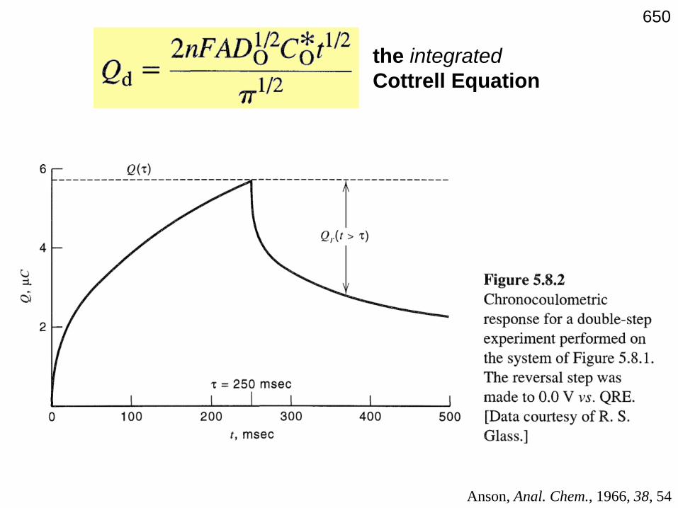
650

the integrated

Cottrell Equation

Anson, Anal. Chem., 1966, 38, 54

651… this is called an Anson plot.

What is this positive intercept?


652

What is this positive intercept?

… this is called an Anson plot.

with ΓO, the surface excess of O (mol cm-2)


653

Fred Anson


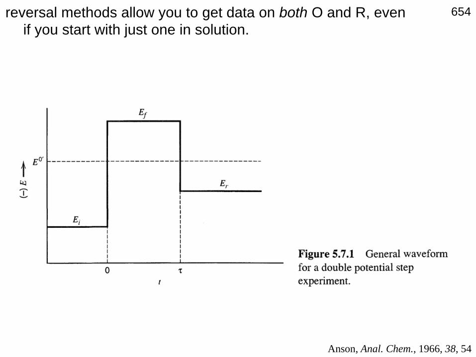
654reversal methods allow you to get data on both O and R, even

if you start with just one in solution.


655

𝑄 𝑡 > 𝜏 =2𝑛𝐹𝐴𝐷𝑅

1/2𝐶𝑅∗ 𝜏1/2 + 𝑡 − 𝜏 1/2 − 𝑡1/2

𝜋1/2+ 𝑄dl + 𝑛𝐹𝐴Γ𝑅

656So, where is the non-ideal data in a Cottrell and Anson plot?

Short times

Long times ?

657… back to one potential step = one data set, from “one” experiment:

experiment observablegoverning

equation

chronoamperometry meas I(t)

chronocoulometry meas Q(t)

658… how else can D be measured? …… how about not using electrochemistry, but NMR… What?

http://chem.ch.huji.ac.il/nmr/techniques/other/diff/diff.html

http://www.ncbi.nlm.nih.gov/pmc/articles/PMC3003887/



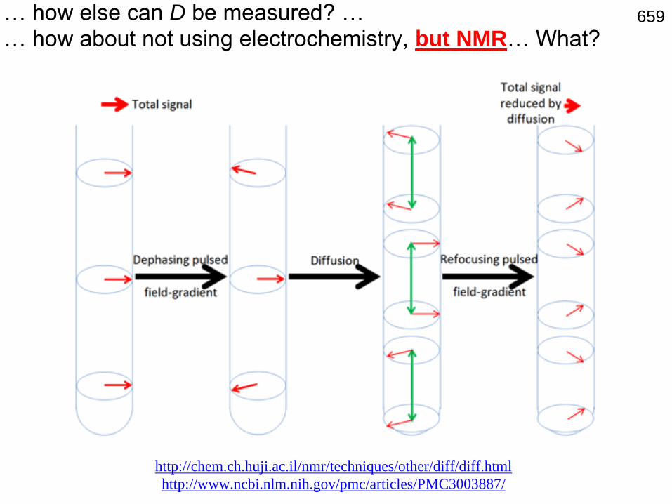
659… how else can D be measured? …… how about not using electrochemistry, but NMR… What?





660

t = 1 st = 0.1 s t = 10 s

insulator

Au

3 mm

planar diffusion mixed diffusionradial

diffusion

How is current affected,

relative to the Cottrell

prediction?

So, back to the limitations… what then physically happens at longer times?

661A typical electrode used in a laboratory electrochemistry experiment

has an area of 0.05 cm2 to 1 cm2.

𝐴 = 𝜋 0.15 2 = 0.0706 cm2 ≈ 7 mm2

662we have equations for the “signal” and the “noise,” so…

we can calculate the signal-to-noise ratio for a potential step experiment

… here we assume

E = 0.6 V, R = 100 Ω

signal

noise

𝒊 =𝑬

𝑹𝒆𝒙𝒑

−𝒕

𝑹𝑪

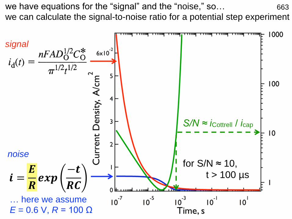
S/N ≈ iCottrell / icap

for S/N ≈ 10,t > 100 µs

663we have equations for the “signal” and the “noise,” so…

we can calculate the signal-to-noise ratio for a potential step experiment

… here we assume

E = 0.6 V, R = 100 Ω

signal

noise

𝒊 =𝑬

𝑹𝒆𝒙𝒑

−𝒕

𝑹𝑪

edge effectscharging

take data

here

664… the RC time constant of the cell imposes a lower limit on the

accessible time window (~100 µs) for a potential step experiment…

… but what is the origin of the long time limit?

… here we assume

E = 0.6 V, R = 100 Ω

signal

noise

𝒊 =𝑬

𝑹𝒆𝒙𝒑

−𝒕

𝑹𝑪

665The Cottrell Equation can be used to describe the behavior during

a potential step experiment as long as the thickness of the diffusion

layer is small relative to the electrode dimension (and, of course,

the boundary layer / stagnant layer / Nernst diffusion layer (δ))…

… So, how long is that?

t (s)

0.1 0.0014 0.009

1 0.0045 0.03

10 0.014 0.09

100 0.045 0.3

Answer: < 1 s

D = 10-5 cm2/s

r0 = 0.15 cm2𝐷𝑡2𝐷𝑡

𝑟0

666

t = 1 st = 0.1 s t = 10 s

insulator

Au

3 mm

linear diffusion mixed diffusionspherical

diffusion



prediction?

When the diffusion layer approaches the dimensions of the electrode

diameter, radial diffusion to the edges of the electrode cause the flux to be

larger than predicted by the Cottrell Equation, and non-uniform.

667

… so in a potential step experiment…

1. current changes continuously with time.

2. radial diffusion (AKA “edge effects”) limit the data

acquisition time window to ~1 s.

3. charging imposes a lower limit of 100 – 500 µs

on this data acquisition time window.

4. maximum current densities are > 60 mA cm-2

initially, but just 100 µA cm-2 at S/N ≈ 10.

… but, why do we care?

668

we need to push this up to perform

meaningful measurements of the

kinetics of fast reactions

Why do we care? One reason…

669

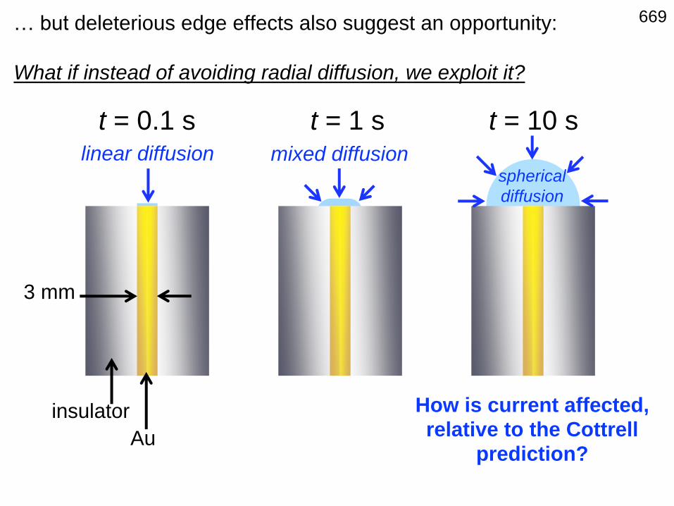
t = 1 st = 0.1 s t = 10 s

insulator

Au

3 mm



prediction?

… but deleterious edge effects also suggest an opportunity:

What if instead of avoiding radial diffusion, we exploit it?

linear diffusion mixed diffusionspherical

diffusion

670

insulator

Au, C, Pt

10 nm – 50 µm

side view top view

… called “ultramicroelectrodes” or “UMEs”

Let’s design an experiment in which we intentionally operate in

this radial diffusion limit the “entire” time!

… well we actually start in the linear regime, and then switch over quickly…

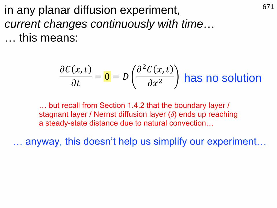
671in any planar diffusion experiment,

current changes continuously with time…

… this means:

has no solution

… anyway, this doesn’t help us simplify our experiment…

… but recall from Section 1.4.2 that the boundary layer / stagnant layer / Nernst diffusion layer (δ) ends up reaching a steady-state distance due to natural convection…

𝜕𝐶 𝑥, 𝑡

𝜕𝑡= 0 = 𝐷

𝜕2𝐶 𝑥, 𝑡

𝜕𝑥2

672

4 µm

14 µm 40 µm

t = 1s

0.1s0.01s0.0001s

… use the geometric area for calculations

C* = 1 x 10-6 M

D = 1 x 10-5 cm2 s-1

2𝐷𝑡 =

… the diffusion layer grows with time (indefinitely)…

673

D = 1.5 x 10-6 cm2 s-1

D = 1 x 10-5 cm2 s-1

… and thus diffusion-controlled currents decay with time (indefinitely)…

the Cottrell

Equation

674

… for a spherical

diffusion field:

and so…

… but the same is not true for purely spherical diffusion:

… which has solutions:

𝜕𝐶 𝑟, 𝑡

𝜕𝑡= 0 = 𝐷

𝜕2𝐶 𝑟, 𝑡

𝜕𝑟2+2

𝑟

𝜕𝐶 𝑟, 𝑡

𝜕𝑟

𝜕𝐶 𝑟, 𝑡

𝜕𝑡=−𝐴

𝑟2𝜕2𝐶 𝑟, 𝑡

𝜕𝑟2=2𝐴

𝑟3

𝐶 𝑟, 𝑡 = 𝐵 +𝐴

𝑟

𝜕𝐶 𝑟, 𝑡

𝜕𝑡= 0 = 𝐷

2𝐴

𝑟3+2

𝑟

−𝐴

𝑟2

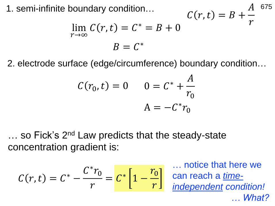
675

2. electrode surface (edge/circumference) boundary condition…

1. semi-infinite boundary condition…

… so Fick’s 2nd Law predicts that the steady-state

concentration gradient is:

… notice that here we

can reach a time-

independent condition!

… What?

𝐶 𝑟, 𝑡 = 𝐵 +𝐴

𝑟

𝐵 = 𝐶∗

lim𝑟→∞

𝐶 𝑟, 𝑡 = 𝐶∗ = 𝐵 + 0

𝐶 𝑟0, 𝑡 = 0 0 = 𝐶∗ +𝐴

𝑟0A = −𝐶∗𝑟0

𝐶 𝑟, 𝑡 = 𝐶∗ −𝐶∗𝑟0𝑟= 𝐶∗ 1 −

𝑟0𝑟

676… the diffusion layer “thickness” is 10r0, no matter how small r0 is!

r0 = 10 µm

1 µm100 nm

10 nm

𝐶 𝑟, 𝑡 = 𝐶∗ 1 −𝑟0𝑟

677… the diffusion layer “thickness” is 10r0, no matter how small r0 is!

r0 = 10 µm

1 µm100 nm

10 nm

… Recall, for transient linear diffusion…

𝐶 𝑟, 𝑡 = 𝐶∗ 1 −𝑟0𝑟

Δ = 2𝑑 𝐷𝑡 =cm2

ss = cm

678the diffusion-limited current pre-factor depends on electrode geometry…

geometry "x"

sphere 4π

hemisphere 2π

disk 4

ringa

b

… but not scan rate!𝑖 = "𝑥"𝑛𝐹𝐷𝐶∗𝑟0

𝜋2 𝑏 + 𝑎

𝑟0 ln 16 𝑏 + 𝑎𝑏 − 𝑎

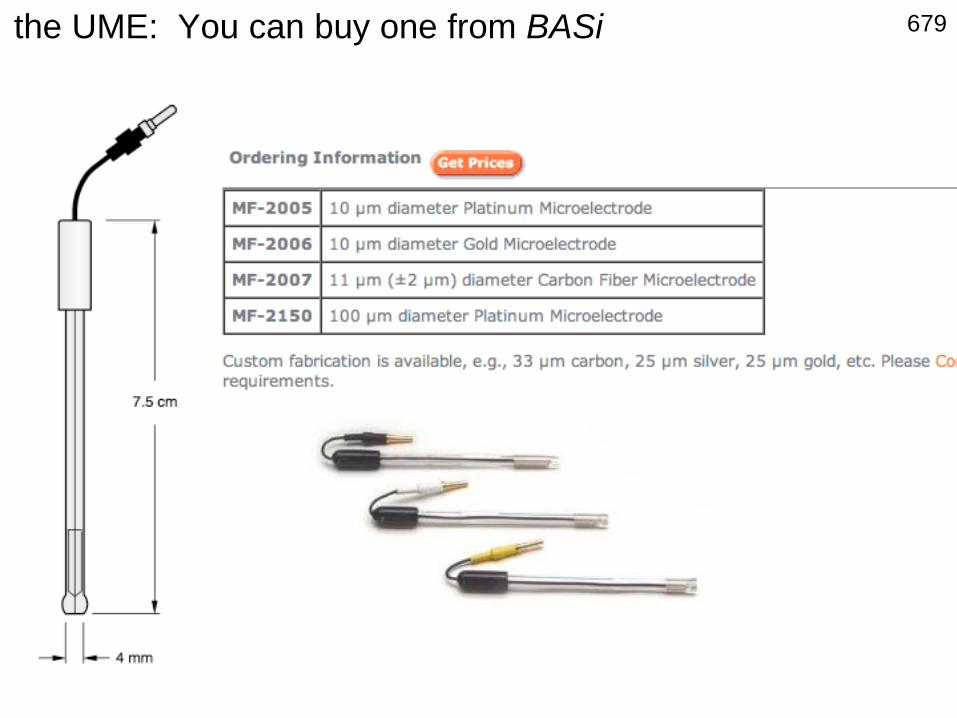
679the UME: You can buy one from BASi

680

Walsh, Lovelock, & Licence, Chem. Soc. Rev., 2010, 39, 4185

… scanning is “often” steady-state at a UME

… steady-state occurs when v << RTD/(nFr02)

681




… v (mV s-1) << 26 mV x (D/r02)

682



… v (mV s-1) << 26 mV x (D/r02)… for a BASi UME with r0 = 5 𝜇m…

… (1 x 10-5 cm2 s-1) / (0.5 x 10-3 cm)2 = 26 x 40 mV s-1s


683





… (1 x 10-5 cm2 s-1) / (0.5 x 10-3 cm)2 = 26 x 40 mV s-1s

… v << 1 V s-1… Wow!

684

Wightman, Anal. Chem., 1981, 53, 1125A




… (1 x 10-5 cm2 s-1) / (0.5 x 10-3 cm)2 = 26 x 40 mV s-1s

… v << 1 V s-1… Wow!

685

Ching, Dudek, & Tabet, J. Chem. Educ., 1994, 71, 602

Documents

Lecture #9 of 18 - UCI Department of Chemistryardo/echem/UCI-CHEM248-2017W_lecture… · use it to measure D! 649 … but what are the problems with this approach? … solution: Integrate