Lecture 9 - KTH · Page 3. Primary and Secondary Data • Primary data ... express connection between concepts • Indicators ... Page 15. Utility theory • Would you like to go

Lecture 9

Methodological questions concerning data, simulations and statistics

Page 1

Some methodology

We will discuss the following:

• Some terminology and facts about data• Some standard methods in statistics• Some methods in computer simulations

Page 2

Data

A part of research is to handle data of different types. It appears that one can describe data in several ways.

• Description after level of abstraction• Split into primary and secondary data• Quantitative and qualitative data• Measurement for different types of scale

Page 3

Primary and Secondary Data

• Primary data - direct measurements or observations of something. Can also be reports of people who themselves have experienced something

• Secondary data - is often compilation of primary data that has been processed in any form. They can e.g. occur in reports, articles or books

Page 4

Quantitative and qualitative data

• Quantitative data - data given in the form of numbers

• Qualitative data - data that can not easily be given in the form of numbers. It may be opinions, stories or descriptions of situations

Page 5

Levels of Abstraction

• Theory - The key interactions expressed in abstract terms

• Concept - The basic concepts. The theory often express connection between concepts

• Indicators - Something measurably which is related to concepts or demonstrate the existence of them

• Variables - The measurable component of the indicators

• Values - the results of measurements of the variables

Page 6

Scientific data and observations

• The previous observations have been such that their values are true / false.

• In other contexts we assign observations a numeric value: observations E1, E2, ..., get the values f (E1), f (E2), ...

• The function f defines the type of scale we use. • What kind of scale you use defines the type of information

one can objectively be read out of the observations.

Page 7

Types of scales

• Ordinal scale : Relations of type f (E1) < f (E2) are significant. An ordinal is just a ranking of the observations.

• Quota Scale: The value f (E2) / f (E1) is significant.

• Interval Scale: value (f (E2) -f (E0)) / (f (E1) -f (E0)) is significant. Typical examples are temperature scales (except Kelvin’s).

Page 8

Collect and analyze secondary data

• Typical examples can be written materials novels, reports, biographies, newspapers, etc.

• It could be television programs, films, interviews, etc.

• It may be statistical surveys made for some other purpose

Page 9

Problems with the analysis

• To find data• To authenticate the sources• Assessing credibility• To determine how representative the data

is• Choosing methods for interpretation of the

data

Page 10

Three methods of analysis

• Content analysis - we simply count the occurrences of something such as words or types of images in the document and use occurrences as indicators

• Data mining - We use software to find patterns in the data

• Meta-analysis - We make an analysis of several other analyzes simultaneously and try to see patterns in them

Page 11

To collect primary dataThe amount of methods is great. However, we can mention three main areas

•Statistical surveys. Sampling.• Interview Methods. •Experiment. Some general methods for experiments is that in addition to the real experimental group we also have a control group. We should also, if possible, use so-called double-blind tests.

Page 12

The 'mathematization' of the world

• One of the reasons for the success of mathematics in science is the possibility of measuring things and then doing mathematical processing of the data.

• This fact can lead to the opinion that only measurable facts can be the subject of science.

• But in Social Sciences it is often claimed that qualitative data are as important as quantitative.

• We will illustrate how it is possible to use how it is possible to use mathematics to define measures on seemingly qualitative and subjective observations.

Page 13

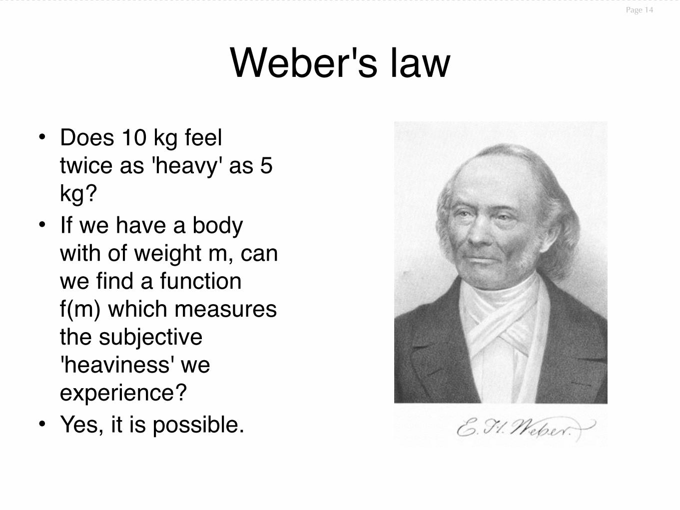
Weber's law• Does 10 kg feel

twice as 'heavy' as 5 kg?

• If we have a body with of weight m, can we find a function f(m) which measures the subjective 'heaviness' we experience?

• Yes, it is possible.

Page 14

Weber's law II• Let dm be the smallest change in mass that we

(subjectively) can detect with our senses.• In the beginning of the 19th century Weber

showed that dm is linearly dependent on m, i.e. dm = cm for some constant m. (In an appropriate interval.)

• From this it is not hard to see that a natural definition of the subjective experience of 'heaviness' has the form k log m + w0 for some constants k, w0.

Page 15

Utility theory• Would you like to go to

an interesting early morning lecture at KTH?

• Or would you rather sleep some hours more?

• Can you measure how much you want different things?

• John von Neumann suggested a way of measuring subjective preferences in an exact way.

Page 16

Utility theory II

• In Game Theory and Mathematical Economics we make the assumption the we can personally order different things a, b, c ,... In preference order.

• We also make the assumption that we can measure how much we want different things by a utility function u.

• This means that we prefer e to q if and only if u(e) > u(q).• How is it possible to define such a function?

Page 17

"What do you chose? 5000 $ or the secret box?"

• The idea von Neumann had was to imagine a virtual lottery. Let a be the thing we prefer most of everything and z the thing we prefer least of everything.

• Now, let L1 be a lottery with two possible outcomes: You get a or you get z. You get a with probability p and z with probability (1-p).

• And then, we take a thing k and imagine a trivial lottery L2 where you get k with certainty.

• Which one do you prefer? L1 or L2? It must depend on p.• There should be a number p such that you are indifferent between L1

and L2. This p is the utility of k, i.e. u(k) = p.• This means that u(a) =1 and u(z) = 0.

Page 18

Is it a realistic measure?• To put it a little extreme, let us say that we want to compare everything. • Let us then assume that a is "Happiness beyond all imagination" and z

is "A horrible and painful death". Let k be "Attending a lecture in The Theory of Science".

• So L1 is the lottery [P(Happiness beyond all imagination) = p, P(A horrible and painful death) = (1-p)]

• And L2 is the lottery [Attending a lecture in The Theory of Science with certainty].

• For what p are you indifferent between L1 and L2?

Page 19

Statistics

KTH/ICTIX1501:F7Göran [email protected]

Page 20

Statistics

• We shall now study the observations of random variables. What values did we get?

• These observations are called one sample (sample). Within the statistics, there are essentially four main areas point estimation interval estimation hypothesis testing Decision Problems

Page 21

Point Estimation• A sample x = {x1, x2, x3, ...} is an observation of stochastic variables

ξ = {ξ1, ξ2, ξ3, …}.

• An estimate is a function f(x) and can be regarded as an observation of f(ξ).

• An estimate of a parameter, µ, is said to be unbiased if the expected value of the estimate is the value of the parameter.

• An estimate is said to be consistent if the difference to the real value goes to 0 as the sample size grows.

Page 22

Confidence Intervals

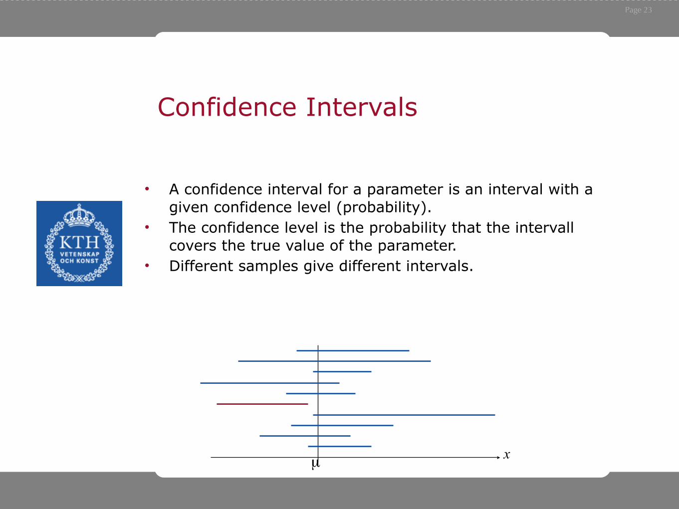
• A confidence interval for a parameter is an interval with a given confidence level (probability).

• The confidence level is the probability that the intervall covers the true value of the parameter.

• Different samples give different intervals.

µ x

Page 23

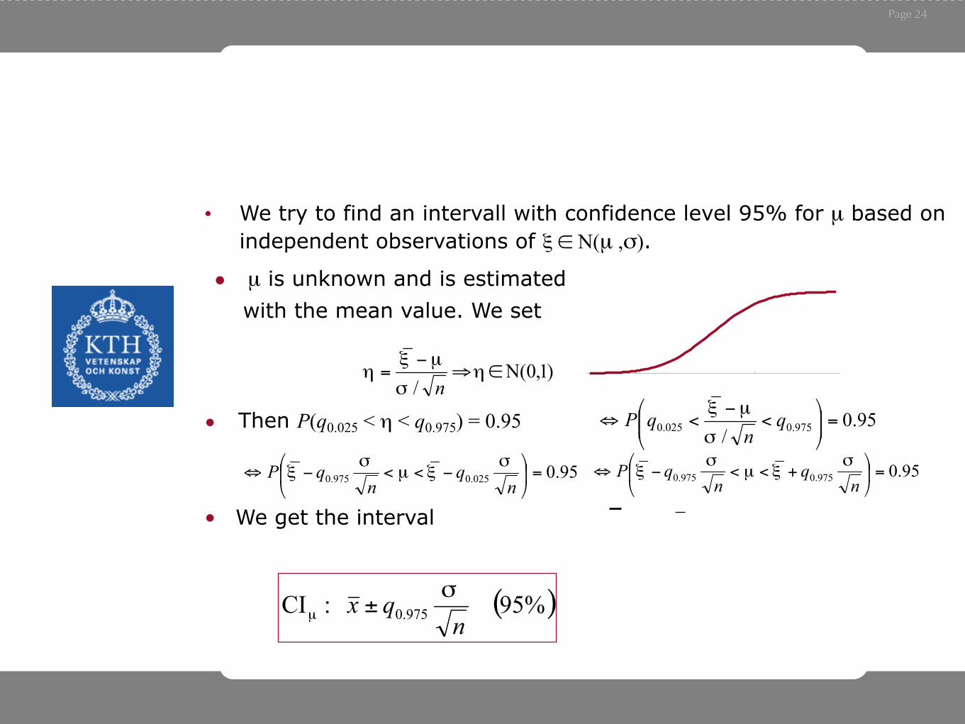
• We try to find an intervall with confidence level 95% for µ based on independent observations of ξ ∈ N(µ ,σ).

• Then P(q0.025 < η < q0.975) = 0.95

)1,0N(/

∈⇒−

= ησ

µξη

n

• µ is unknown and is estimated with the mean value. We set

95.0/ 975.0025.0 =!!

"

#$$%

&<

−<⇔ q

nqP

σ

µξ

95.0025.0975.0 =!"

#$%

&−<<−⇔

nq

nqP σ

ξµσ

ξ 95.0975.0975.0 =!"

#$%

&+<<−⇔

nq

nqP σ

ξµσ

ξ

• We get the interval

qax

aFHxL

( )%95 :CI 975.0 nqx σ

µ ±

Page 24

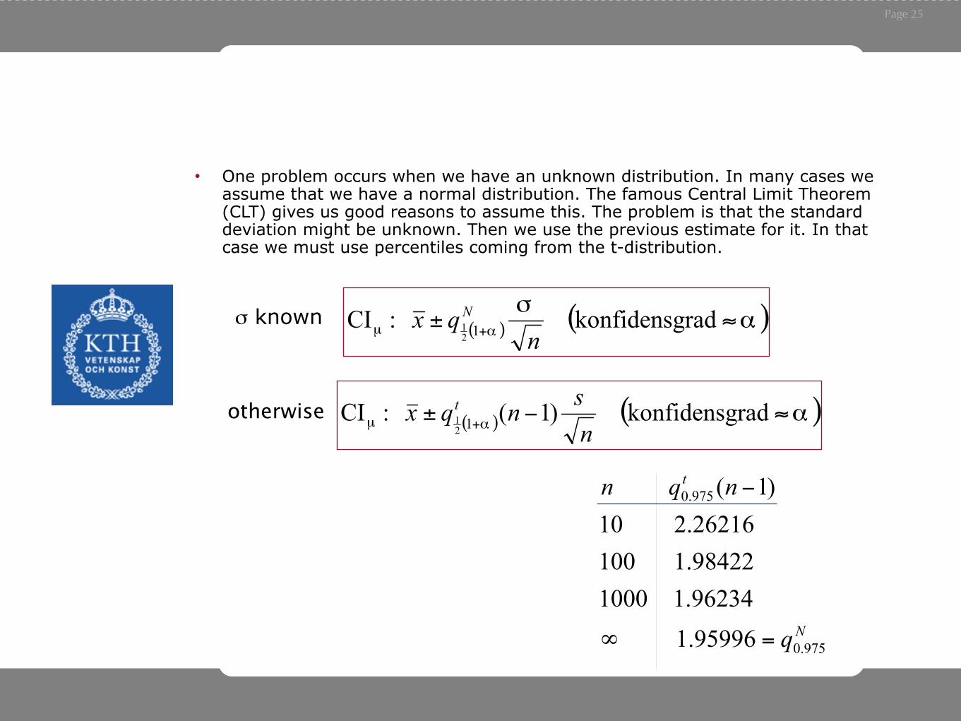
• One problem occurs when we have an unknown distribution. In many cases we assume that we have a normal distribution. The famous Central Limit Theorem (CLT) gives us good reasons to assume this. The problem is that the standard deviation might be unknown. Then we use the previous estimate for it. In that case we must use percentiles coming from the t-distribution.

otherwise ( ) ( )ααµ ≈−± + radkonfidensg)1( :CI 121

nsnqx t

( ) ( )ασαµ ≈± + radkonfidensg :CI 12

1

nqx Nσ known

N

t

q

nqn

975.0

975.0

1.959961.9623400011.98422 0012.2621610

)1(

=∞

−

Page 25

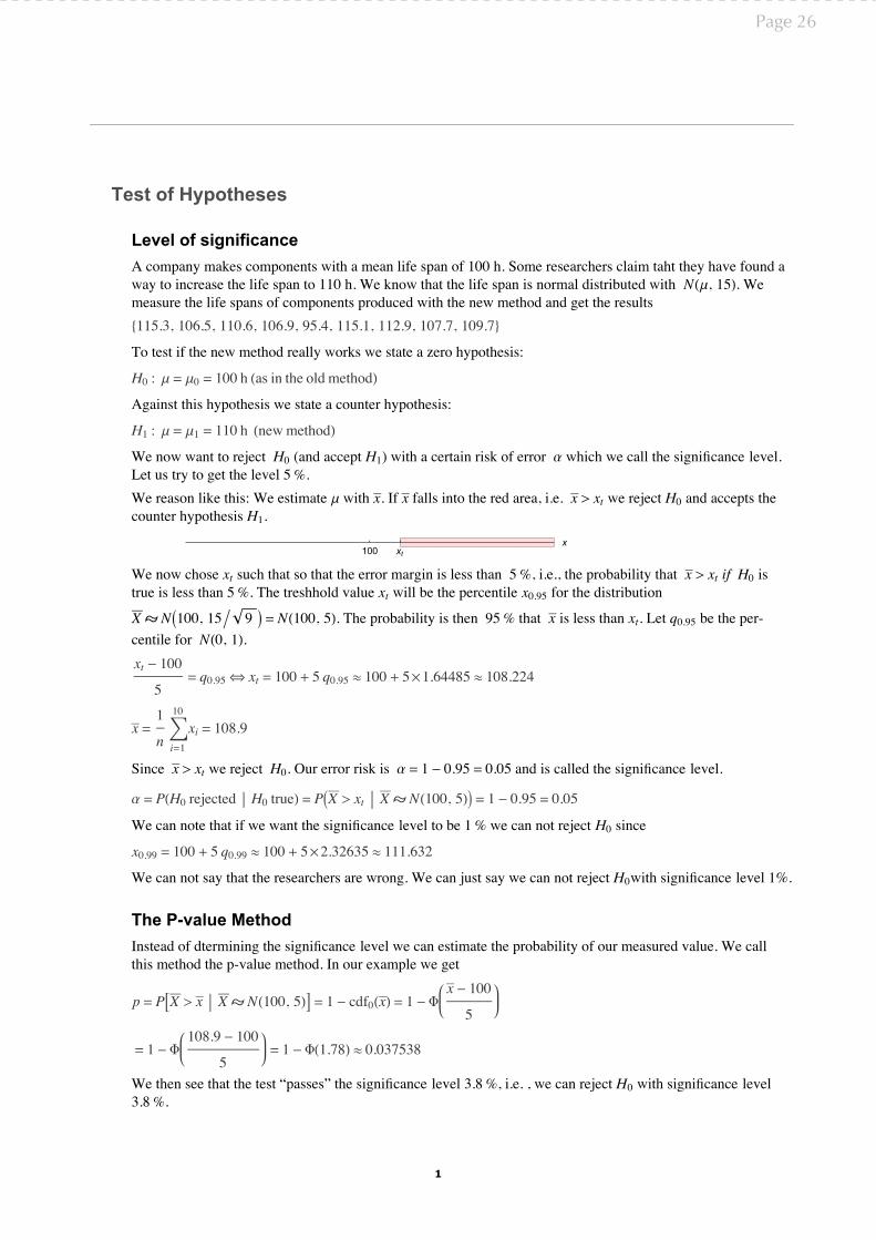
Test of Hypotheses

Level of significance��(μ� ��)��{�� }

��

�� μ = μ� = �� (�� )

��

�� μ = μ� = �� (��)

��α��%��μ�� > ��

100 xtx

��%�� > ��%��

� � �� = �(�� )��%��(�� )�� - ��

�= ��⇔ �� = �� + � �� ≈ �� + �×�� ≈ ��

� =�

� �=�

��

�� = ��

�� > ��α = � - �� = ��

α = �(�� ) = � � > �� (�� ) = � - �� = ��

��%��

�� = �� + � �� ≈ �� + �×�� ≈ ��

��

The P-value Method��

� = � � > � � �(�� ) = � - ��(�) = � - Φ� - ��

�

= � - Φ�� - ��

�= � - Φ(��) ≈ ��

��“��”��%��%�

1

Page 26

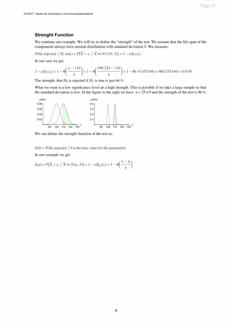
Strenght Function��“��”��

�(�� ) = � � > �� (�� ) = � - ��(��)

��

� - ��(��) = � - Φ�� - ��

�≈ � - Φ

�� - ��

�≈ � - Φ(-��) = Φ(��) ≈ ��

��%�

�� = ��×��%�

90 100 110 120 130x

0.02

0.04

0.06

0.08

pdf(x)

90 100 110 120 130x

0.1

0.2

0.3

0.4

pdf(x)

��

�(θ) = �(�� θ �� )

��

�(μ) = � � > �� (μ� �) = � - ��μ(��) = � - Φ�� - μ

�

KTH/ICT - Skolan för informations- och kommunikationsteknik

2

Page 27

Computer SimulationsThere is one area of science that is probably relatively unexplored: The Philosophy of Computer Simulation.

Normally we observe reality and make observations. We can use computer methods to analyze data.

But we can make computer simulations of ”reality” instead.

Page 28

A formal aspect of computer methods

Let us assume that we have a process P that we want to simulate

• We might believe that we understand the process• We the try to write a program simulating the process• When we write the program we might run into

difficulties which forces us to rethink our understanding of the process

• So even without running the program we might gain understanding of the model in which the process is living in

Page 29

Example:The Monty Hall Problem

Suppose you're on a game show, and you're given the choice of three doors: Behind one door is a car; behind the others, goats. You pick a door, say No. 1, and the host, who knows what's behind the doors, opens another door, say No. 3, which has a goat. He then says to you, "Do you want to pick door No. 2?" Is it to your advantage to switch your choice?

Page 30

Solution?

It is said that it is to your advantage to alter your choice. Do you believe it. Some think it is impossible. But there are formal proofs that it is.

What to believe? Can we test it in ”reality”?

Page 31

Computer Simulation

Let us try to write a program that tests if it is a good strategy to alter your choice. How do you design a program.

• There are some random components. • Then there are some assumptions of the

choices the actors (two) make.

Page 32

Some detailsHere are some steps:

• You distribute the car and the goats randomly• The guest choses randomly• Then you have to simulate the host’s acting. What does the

host know. What strategy does he use? - This is a critical point

• Then the simulation of the guest is simple - just change door

• Run this many times. Count the number of times the guest wins the car.

• Make the same simulation when the guest does not change door. Result?

Page 33

Documents

Lecture 9 - KTH · Page 3. Primary and Secondary Data • Primary data ... express connection between concepts • Indicators ... Page 15. Utility theory • Would you like to go