Les Cahiers du GERAD ISSN: 0711–2440

Employee scheduling with short demandperturbations and extensible shifts

R. Burgy, H. Michon-Lacaze,G. Desaulniers

G–2018–18

March 2018

La collection Les Cahiers du GERAD est constituee des travaux derecherche menes par nos membres. La plupart de ces documents detravail a ete soumis a des revues avec comite de revision. Lorsqu’undocument est accepte et publie, le pdf original est retire si c’estnecessaire et un lien vers l’article publie est ajoute.

Citation suggeree: R. Burgy, H. Michon-Lacaze, G. Desaulniers(Mars 2018). Employee scheduling with short demand perturbationsand extensible shifts, document de travail, Les Cahiers du GERADG-2018-18, GERAD, HEC Montreal, Canada.

Avant de citer ce rapport technique, veuillez visiter notre site Web(https://www.gerad.ca/fr/papers/G-2018-18) afin de mettre a jourvos donnees de reference, s’il a ete publie dans une revue scientifique.

The series Les Cahiers du GERAD consists of working papers carriedout by our members. Most of these pre-prints have been submitted topeer-reviewed journals. When accepted and published, if necessary, theoriginal pdf is removed and a link to the published article is added.

Suggested citation: R. Burgy, H. Michon-Lacaze, G. Desaulniers(March 2018). Employee scheduling with short demand perturbationsand extensible shifts, Working paper, Les Cahiers du GERAD G-2018-18,GERAD, HEC Montreal, Canada.

Before citing this technical report, please visit our website (https://www.gerad.ca/en/papers/G-2018-18) to update your reference data,if it has been published in a scientific journal.

La publication de ces rapports de recherche est rendue possible grace ausoutien de HEC Montreal, Polytechnique Montreal, Universite McGill,Universite du Quebec a Montreal, ainsi que du Fonds de recherche duQuebec – Nature et technologies.

Depot legal – Bibliotheque et Archives nationales du Quebec, 2018– Bibliotheque et Archives Canada, 2018

The publication of these research reports is made possible thanks to thesupport of HEC Montreal, Polytechnique Montreal, McGill University,Universite du Quebec a Montreal, as well as the Fonds de recherche duQuebec – Nature et technologies.

Legal deposit – Bibliotheque et Archives nationales du Quebec, 2018– Library and Archives Canada, 2018

GERAD HEC Montreal3000, chemin de la Cote-Sainte-Catherine

Montreal (Quebec) Canada H3T 2A7

Tel. : 514 340-6053Telec. : 514 340-5665info@gerad.cawww.gerad.ca

Employee scheduling with short demand perturbations andextensible shifts

Reinhard Burgy a

Helene Michon-Lacaze b

Guy Desaulniers a

a GERAD & Departement de Mathematiques et deGenie Industriel, Polytechnique Montreal, Montreal(Quebec), Canada

b GERAD & Ubisoft, Montreal (Quebec), Canada

reinhard.burgy@gerad.ca

helene.michon-lacaze@ubisoft.com

guy.desaulniers@gerad.ca

March 2018Les Cahiers du GERADG–2018–18Copyright c© 2018 GERAD, Burgy, Michon-Lacaze, Desaulniers

Les textes publies dans la serie des rapports de recherche Les Cahiers duGERAD n’engagent que la responsabilite de leurs auteurs. Les auteursconservent leur droit d’auteur et leurs droits moraux sur leurs publica-tions et les utilisateurs s’engagent a reconnaıtre et respecter les exigenceslegales associees a ces droits. Ainsi, les utilisateurs:• Peuvent telecharger et imprimer une copie de toute publication

du portail public aux fins d’etude ou de recherche privee;

• Ne peuvent pas distribuer le materiel ou l’utiliser pour une ac-tivite a but lucratif ou pour un gain commercial;

• Peuvent distribuer gratuitement l’URL identifiant la publication.Si vous pensez que ce document enfreint le droit d’auteur, contactez-nous en fournissant des details. Nous supprimerons immediatementl’acces au travail et enqueterons sur votre demande.

The authors are exclusively responsible for the content of their researchpapers published in the series Les Cahiers du GERAD. Copyright andmoral rights for the publications are retained by the authors and the usersmust commit themselves to recognize and abide the legal requirementsassociated with these rights. Thus, users:• May download and print one copy of any publication from the

public portal for the purpose of private study or research;

• May not further distribute the material or use it for any profit-making activity or commercial gain;

• May freely distribute the URL identifying the publication.If you believe that this document breaches copyright please contact usproviding details, and we will remove access to the work immediatelyand investigate your claim.

ii G–2018–18 Les Cahiers du GERAD

Abstract: Employee scheduling is an important activity in the service industry as it has a significantimpact on costs, sales, and profitability. While a large amount of mathematical models and methods havebeen established in the literature for finding optimized schedules, only few propose optimization methodsfor practically relevant problem settings including uncertainty, which is an important aspect of employeescheduling in the service industry.

This article contributes to narrowing this research gap by addressing a practice-inspired employee schedul-ing problem arising in retail stores. In particular, the scheduling problem under study includes short demandperturbations, potentially leading to an increase of the demand in some time intervals, and the possibilityof assigning overtime work by extending shifts to cope with a lack of employees in real-time. The goal isto find an initial schedule minimizing the sum of demand fulfillment and employee preference-related costs,where each cost term is expressed as a convex function of an appropriate variable. The cost of a schedule isevaluated using a simulation-based approach reproducing the materialization of demand perturbations andshift extensions.

In order to find reasonably good robust employee schedules within a relatively short computation timefor practical-sized instances, we propose two integer programming models taking into account the demanduncertainty and shift extension possibilities in different ways. In the first model, a bonus term is assignedin the objective function for shifts that can cover some perturbation demand within their extension period,while in the second model, a potential demand is derived from the perturbations and its under-coverage ispenalized. Extensive computational results on retail store instances reveal that the two proposed robustmodels improve the schedule quality significantly when compared with a basic non-robust model. Thisresult further underpins the value of including uncertainty information and recourse actions in the employeescheduling activity.

Keywords: Employee scheduling, demand uncertainty, shift extension, simulation-based cost estimation,integer programming

Acknowledgments: This work was funded by Kronos Canadian Systems and the Natural Sciences andEngineering Research Council (NSERC) of Canada under grant #RDCPJ 468 716-14. The financial sup-port is greatly appreciated. The authors are also grateful to Kronos Canadian Systems for proposing theproblem under study and for providing the data sets. Special thanks go to Francois Lessard who helped inimplementing the solution approach.

Les Cahiers du GERAD G–2018–18 1

1 Introduction

An employee work schedule specifies all employees’ work time intervals and assigned duties, also called jobs,

for some specified time horizon. Personnel scheduling, which is the process of building and updating work

schedules, is a recurrent activity in all types of organizations, and managers dedicate a significant amount

of time and effort to this process. The specific personnel scheduling problems vary from one organization

to another as they are shaped by the organizations’ unique characteristics and needs, such as the hours of

operations, demand patterns, job types and employee skills, possible shift start and end times, break and

rest considerations, and labor agreements. Consequently, a large number of different personnel scheduling

problems have been established in the literature. There are, for example, a number of studies dealing with

staff scheduling in hospitals (Wright and Mahar, 2013; Legrain et al., 2015), call centers (Aksin et al., 2007;

Dietz, 2011), airlines (Desaulniers et al., 1998; Kasirzadeh et al., 2017), retail stores (Lam et al., 1998; Kabak

et al., 2008), restaurants (Love Jr. and Hoey, 1990; Hur et al., 2004), and postal services (Bard et al., 2003;

Brunner and Bard, 2013).

The employee scheduling process is of particular importance in the retail industry, which is considered in

this article, as labor scheduling has a substantial impact on costs, sales, and profitability (Perdikaki et al.,

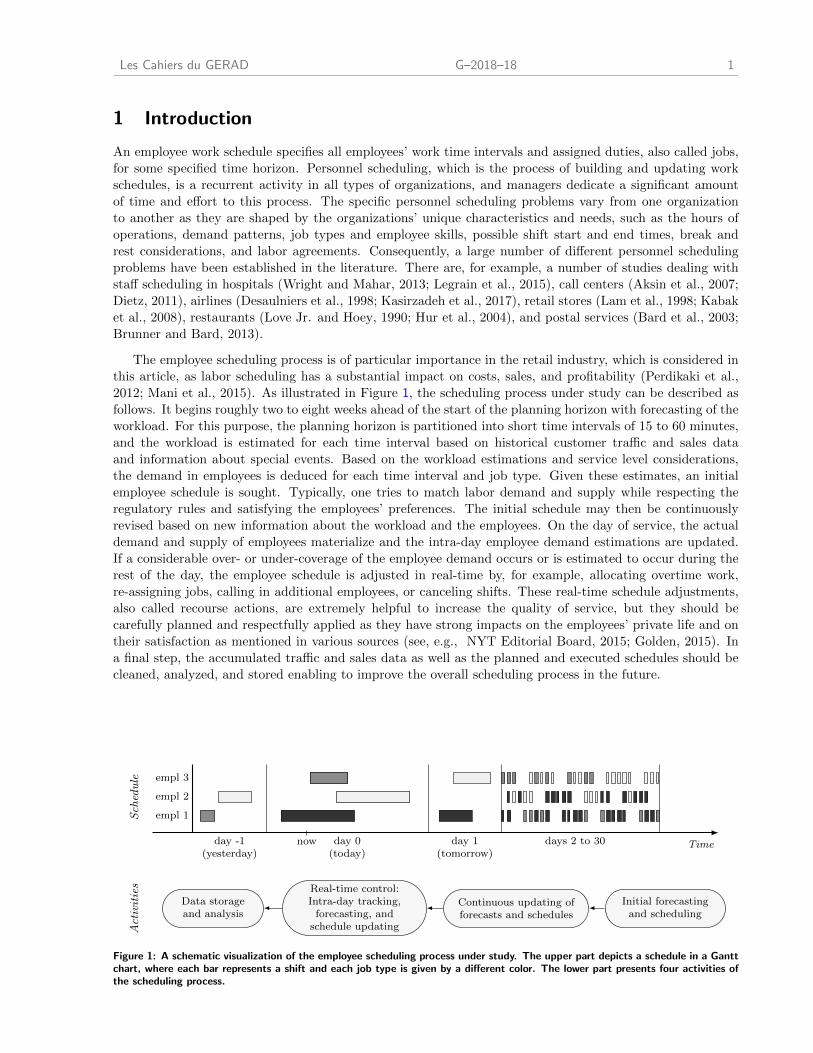
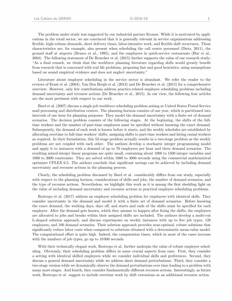
2012; Mani et al., 2015). As illustrated in Figure 1, the scheduling process under study can be described as

follows. It begins roughly two to eight weeks ahead of the start of the planning horizon with forecasting of the

workload. For this purpose, the planning horizon is partitioned into short time intervals of 15 to 60 minutes,

and the workload is estimated for each time interval based on historical customer traffic and sales data

and information about special events. Based on the workload estimations and service level considerations,

the demand in employees is deduced for each time interval and job type. Given these estimates, an initial

employee schedule is sought. Typically, one tries to match labor demand and supply while respecting the

regulatory rules and satisfying the employees’ preferences. The initial schedule may then be continuously

revised based on new information about the workload and the employees. On the day of service, the actual

demand and supply of employees materialize and the intra-day employee demand estimations are updated.

If a considerable over- or under-coverage of the employee demand occurs or is estimated to occur during the

rest of the day, the employee schedule is adjusted in real-time by, for example, allocating overtime work,

re-assigning jobs, calling in additional employees, or canceling shifts. These real-time schedule adjustments,

also called recourse actions, are extremely helpful to increase the quality of service, but they should be

carefully planned and respectfully applied as they have strong impacts on the employees’ private life and on

their satisfaction as mentioned in various sources (see, e.g., NYT Editorial Board, 2015; Golden, 2015). In

a final step, the accumulated traffic and sales data as well as the planned and executed schedules should be

cleaned, analyzed, and stored enabling to improve the overall scheduling process in the future.

Time

empl 1

empl 2

empl 3

day -1(yesterday)

day 0(today)

now day 1(tomorrow)

days 2 to 30

Activities

Schedule

Initial forecastingand scheduling

Continuous updating offorecasts and schedules

Real-time control:Intra-day tracking,forecasting, and

schedule updating

Data storageand analysis

Figure 1: A schematic visualization of the employee scheduling process under study. The upper part depicts a schedule in a Ganttchart, where each bar represents a shift and each job type is given by a different color. The lower part presents four activities ofthe scheduling process.

2 G–2018–18 Les Cahiers du GERAD

The initial schedule generation is an important activity in the scheduling process as it largely defines the

quality of the final schedule. Since it must be executed quite a long time ahead, a considerable amount of

uncertainty is involved in this step, especially with respect to the demand of employees. When establishing

the initial schedule, this demand is typically expressed as a point estimate for each time interval and the

possible recourse actions are not considered. Therefore, expensive recourse actions for which the schedule

is not optimized for could be necessary to cope with a labor shortage or surplus in real-time. Indeed, it

has been shown that schedules optimized with respect to demand uncertainty and recourse actions lead to

a significant reduction of the actual labor costs, to an improvement in customer service levels, and to more

satisfied employees (Bard et al., 2007; Kim and Mehrotra, 2015; Parisio and Jones, 2015; Restrepo et al.,

2017). Hence, schedule robustness deserves special attention in the initial employee scheduling activity.

This article contributes to the line of research on robust employee scheduling by addressing the following

optimization problem arising in the initial scheduling phase. Multi-skilled employees must be assigned to

perform various jobs over a planning horizon of one week, which is partitioned into small consecutive time

intervals of 15 minutes. For each job and time interval, a demand in employees is given. In addition, one

can specify short perturbations of this demand. A perturbation materializes with a given probability, and

it increases the basic demand of a specific job by a given amount of employees in a prespecified short time

interval if it materializes. This type of perturbation makes it possible to model situations in which the

demand of employees is particularly uncertain in given time periods. Such a perturbation may, for example,

be used to model the demand uncertainty related to peak hours, which is a relevant source of uncertainty

(Mani et al., 2015). Another application is related to the uncertainty caused by weather (Agnew and Thornes,

1995). Grocery stores, for example, may experience higher demand at lunch time in bad weather conditions.

Each employee is qualified to perform certain jobs and has specific work time preferences and total work time

restrictions per day and week. An employee can be assigned to at most one mono-job work shift per day,

and the rest period between two consecutive shifts of an employee must be of a minimum length. Breaks

within shifts, for example lunch breaks, are not modeled explicitly. We assume that they are assigned to

the employees in real-time depending on the observed demand, and are considered in the planning phase

by slightly increasing the demand forecasts in certain time intervals. In order to cope with the demand

uncertainty in real-time, we allow to postpone the end of a shift, so extending it, by at most one hour. This

is one of the most used, simplest, and cheapest recourse actions available in practice to shortly increase the

number of employees. When a perturbation materializes, we decide in real-time which shifts to extend. The

quality of a schedule is measured by the sum of demand fulfillment and employees’ work time preference-

related costs. Hereby, each cost term is expressed as a convex function of an appropriate variable capturing

the demand fulfillment or employee preferences. Compared to a simpler linear function, the convex shape

enables a more accurate modeling of the decision problem at hand as it makes it possible to increase the

unit penalties with increasing variable value. We evaluate the actual cost of a schedule with a simulation-

based approach. For this purpose, we first generate a large number of scenarios based on the demand and

perturbation information, then simulate the materialization of the perturbations and the extension of shifts,

and finally compute the total cost of the so-obtained schedule with respect to the actual demand. Note

that the salaries of the employees are not considered directly. However, the over-coverage costs prevent from

unnecessary overstaffing, and the minimum work time specifications can be used to distribute the work load

among the employees as desired.

We aim at developing approaches that find reasonably good (initial) employee schedules within a relatively

short computation time for practical-sized instances. In particular, our computational tests are executed

on instances with up to 40 employees and seven jobs, and the computation time limit is one hour. Our

approaches rely on the modeling of the employee scheduling problem as integer linear programs. We first

discuss a basic employee scheduling model that does not include the demand uncertainty, and then develop

two different models dealing with the uncertainty and recourse actions in different ways. Both are, however,

not fully representing the multi-stage stochastic aspects of the scheduling problem as this would typically

yield models that are extremely difficult to solve with current state-of-the-art algorithms. Note that the

demand forecasting step is not discussed here, and we refer the reader to the works of Shen and Huang

(2008) and Mehrotra et al. (2010) for a comprehensive treatment of it.

Les Cahiers du GERAD G–2018–18 3

The problem under study was suggested by our industrial partner Kronos. While it is motivated by appli-

cations in the retail sector, we are convinced that it is generally relevant in service organizations addressing

flexible, high-volume demands, short delivery times, labor-intensive work, and flexible shift structures. These

characteristics are, for example, also present when scheduling the call center personnel (Dietz, 2011), the

ground staff at airports (Brusco et al., 1995), and the employees in quick-service restaurants (Hur et al.,

2004). The following statement of De Bruecker et al. (2015) further supports the value of our research study:

“As a final remark, we think that the workforce planning literature regarding skills would greatly benefit

from research that is concerned with real life problems, proposing fast and good heuristics, using assumptions

based on sound empirical evidence and does not neglect uncertainty.”

Literature about employee scheduling in the service sector is abundant. We refer the reader to the

reviews of Ernst et al. (2004), Van Den Bergh et al. (2013) and De Bruecker et al. (2015) for a comprehensive

overview. However, only few contributions address practice-related employee scheduling problems including

demand uncertainty and recourse actions (De Bruecker et al., 2015). In our view, the following four articles

are the most pertinent with respect to our work.

Bard et al. (2007) discuss a single-job workforce scheduling problem arising at United States Postal Service

mail processing and distribution centers. The planning horizon consists of one year, which is partitioned into

intervals of one hour for planning purposes. They model the demand uncertainty with a finite set of demand

scenarios. The decision problem consists of the following stages. At the beginning, the shifts of the full-

time workers and the number of part-time employees must be specified without knowing the exact demand.

Subsequently, the demand of each week is known before it starts, and the weekly schedules are established by

allocating overtime to full-time workers’ shifts, assigning shifts to part-time workers and hiring casual workers

as required. In their formulation, this 52-stage problem actually results in a two-stage problem as the weekly

problems are not coupled with each other. The authors develop a stochastic integer programming model

and apply it to instances with a demand of up to 70 employees per hour and three demand scenarios. The

resulting mixed-integer linear programs are quite small, containing about 1000 to 1500 integer variables and

1000 to 2000 constraints. They are solved within 1000 to 4000 seconds using the commercial mathematical

optimizer CPLEX 6.5. The authors conclude that significant savings can be achieved by including demand

uncertainty and recourse actions in the planning process.

Clearly, the scheduling problem discussed by Bard et al. considerably differs from our study, especially

with respect to the planning horizon, considerations of skills and jobs, the number of demand scenarios, and

the type of recourse actions. Nevertheless, we highlight this work as it is among the first shedding light on

the value of including demand uncertainty and recourse actions in practical employee scheduling problems.

Restrepo et al. (2017) address an employee scheduling problem for employees with identical skills. They

consider uncertainty in the demand and model it with a finite set of demand scenarios. Before knowing

the exact demand, the working days, days off, and starts and ends of the shifts must be specified for each

employee. After the demand gets known, which they assume to happen after fixing the shifts, the employees

are allocated to jobs and breaks within their assigned shifts are included. The authors develop a multi-cut

L-shaped solution approach, and discuss experiments on weekly instances with up to five job types, 128

employees, and 100 demand scenarios. Their solution approach provides near-optimal, robust solutions that

significantly reduce labor costs when compared to solutions obtained with a deterministic mean-value model.

The computational effort is quite high. Indeed, the computation times, which in most of the cases increase

with the numbers of job types, go up to 10 000 seconds.

With their technically elegant work, Restrepo et al. further underpin the value of robust employee sched-

uling. Obviously, their scheduling problem differs in some crucial aspects from ours. First, they consider

a setting with identical skilled employees while we consider individual skills and preferences. Second, they

discuss a general demand uncertainty while we address short demand perturbations. Third, they consider a

two-stage version while we dynamically observe the demand perturbations over time leading to a problem with

many more stages. And fourth, they consider fundamentally different recourse actions. Interestingly, as future

work, Restrepo et al. suggest to include overtime work by shift extensions as an additional recourse action.

4 G–2018–18 Les Cahiers du GERAD

Pacqueau and Soumis (2014) discuss a single job, anonymous shift scheduling problem with a one-day

(24-hour) time horizon partitioned into 96 intervals of 15 minutes. They consider demand uncertainty with a

finite set of scenarios. The optimization problem consists of two stages: Without knowing the exact demand,

full-time shifts are allocated in a first stage, while recourse actions are assigned after the exact demand

gets known in a second stage. The set of recourse actions comprises hiring part-time workers, introducing

one or two hours of overtime work to full-time shifts, and allocating breaks to assigned shifts. The authors

develop a heuristic adaption of the L-shaped method capable of finding excellent solutions within one hour of

computation time for instances with up to 500 demand scenarios resulting in models with 10 million integer

variables.

Pacqueau and Soumis deal with an employee scheduling problem arising in the same industries as our

study. However, they consider a more general demand uncertainty and a larger set of recourse actions but a

simpler setting with respect to the time horizon, jobs, employee preferences, and number of decision stages.

Interestingly, their heuristic finds excellent solutions for their extremely large stochastic model within reason-

able computation times. In line with the previously discussed studies, the stochastic modeling approach yields

substantial savings and more robust solutions with respect to the solution quality over a deterministic model.

Parisio and Jones (2015) address a weekly multi-skilled employee scheduling problem arising at a retail

outlet. Uncertainty of the demand is considered by including random forecast errors and deriving a set of

representative demand scenarios from these values. The aim is to find a schedule minimizing the squared

norm of the demand under- and over-coverage. The authors consider two versions: The first includes no

recourse actions while the second allows to extend shifts by one hour after observing the true demand. They

formulate the employee scheduling problem as a two-stage stochastic model, solve it with CPLEX 12.0, and

report results for a retail outlet with 13 employees. Optimal solutions are obtained within a computation

time of about 4500 seconds. The authors conclude that the stochastic variants substantially improve the

quality of the schedule when compared to results obtained with a deterministic mean-value model. However,

they see no meaningful improvement of the schedule quality when including the shift extension possibility.

The scheduling problem introduced by Parisio and Jones shares many features with the one we propose

here, especially in terms of work restrictions, employee preferences and recourse actions. Interestingly and

somewhat in contrast to their results, we will show that the possibility of extending shifts has a significant

impact on the schedule quality. This discrepancy may be due to the different uncertainty modeling. Indeed,

short demand perturbations may be absorbed by positioning shifts well in time, while it is certainly more

difficult to make use of the shift extensions when dealing with forecast error-based demand scenarios.

We conclude this section by a short summary of our contributions. We propose a novel way to include and

tackle uncertainty and recourse actions in a service employee scheduling problem. While most contributions

deal with more generic stochastic problems, typically resulting in computationally heavy optimization models,

our perturbation-based uncertainty models produce a relatively small computational overhead when compared

to the deterministic counterpart. This lightweight approach is particularly important as we include the

employees’ characteristics and preferences in a fine-grained manner, which is important from an application

point of view but usually results in practically intractable optimization problems when combined with a

generic scenario-based demand uncertainty. Our numerical results further shed light on the value of including

uncertainty and recourse actions into the employee scheduling problems.

The remaining part of this paper is organized as follows. The next section formally introduces the

employee scheduling problem. Section 3 presents three integer programming models that can be used to find

optimized employee schedules. These models, which can be solved by a mixed-integer linear programming

solver, are evaluated with extensive computational experiments in Section 4, and a conclusion is provided in

Section 5.

Les Cahiers du GERAD G–2018–18 5

2 The employee scheduling problem with demand perturbations andextensible shifts

The employee scheduling problem considered here can be defined formally as follows. Consider a set J of

jobs, a set E of employees and a planning horizon of one week composed of days D1 to D7. We divide the

planning horizon into consecutive intervals of 15 minutes and introduce an ordered set I = {i1, . . . , i|I|}comprising the resulting time intervals, where ir denotes the rth interval in set I. We will typically use i

without an index to refer to a generic interval in I. Each interval i ∈ I starts and ends at a specific day

day(i) ∈ {D1, . . . , D7} of the week. In the sequel, all time lengths are specified in units of time intervals.

A demand dij in employees is given for each time interval i ∈ I and job j ∈ J . This demand can be

increased by perturbations described in set P. Each perturbation p ∈ P has a probability pr(p) ∈ ]0, 1[ of

materialization. If it materializes, it increases the demand of job(p) ∈ J by inc(p) ∈ Z>0 employees from

the start of time interval sta(p) ∈ I to the end of time interval end(p) ∈ I. Hence, a perturbation p ∈ P is

best described by a tuple p = (pr(p), job(p), inc(p), sta(p), end(p)). Denote by I(p) the set of time intervals

that are possibly affected by perturbation p. We assume that whether a perturbation materializes is known

one time interval before its start. As longer perturbations usually call for other recourse actions than the

short shift extensions integrated here, we will only consider short perturbations with a length of four time

intervals. In principle, we could define perturbations affecting the same job that overlap in time. However,

we will only discuss the non-overlapping case, i.e., where I(p)∩ I(p′) = ∅ holds for all distinct p, p′ ∈ P with

job(p) = job(p′), as, in our view, the specification of overlapping perturbations is rarely useful and slightly

complicates some notational elements.

The following data is given for each employee e ∈ E : a set of job qualifications, a minimum and maximum

(daily) shift length, a maximum total number of shifts denoted by ne, a minimum rest length re between any

two executed shifts, a minimum total work time tmine and a maximum total work time tmax

e . While the total

work time must be at most tmaxe , it can be smaller than tmin

e . However, deviations from this minimal value are

penalized in the objective function. Furthermore, the employee’s work time preferences are specified by a set

Iune ⊆ I of intervals in which the employee is unavailable or does not wish to work and a set of preferred inter-

vals Iprefe ⊆ I. All other intervals, i.e., I\(Iun

e ∪Iprefe ), belong to set Iav

e in which employee e is simply available.

Based on the demand and employee specifications, a large set S of personalized employee shifts is gen-

erated. Each shift s ∈ S specifies an employee emp(s) ∈ E working on a job(s) ∈ J from the start of

time interval sta(s) ∈ I to the end of time interval end(s) ∈ I. Hence, a shift can be specified by a tuple

s = (emp(s), job(s), sta(s), end(s)). For any employee e ∈ E , denote by set S(e) all shifts s ∈ S associated

with employee e = emp(s), and for any shift s, let I(s) be the set comprising all time intervals within shift

s including sta(s) and end(s). A shift s is called feasible if employee emp(s) can accomplish job(s) and the

shift length respects the minimum and maximum shift length restrictions of emp(s). Only feasible shifts are

generated. Due to confidentiality reasons, we omit the details of the shift generation process. Some statistical

data is, nevertheless, provided in Section 4.

An employee schedule is obtained by selecting a subset S of shifts from S that are actually executed. A

schedule S is feasible if each employee e ∈ E is associated with at most ne shifts in S, the minimum rest

length re between each pair of consecutive shifts of e in S is satisfied, and the total work time of e in S is

not larger than tmaxe .

In order to cope with the additional demand arising from materialized perturbations, we allow to slightly

change a schedule S during its execution by taking the following recourse actions. Each shift s ∈ S can be

extended by at most four time intervals, i.e., the end of s can be postponed by at most one hour. However,

the feasibility of the so-obtained schedule must be preserved. For example, an extended shift s must respect

the maximum shift length of employee e = emp(s), and the employee’s next shift must not start earlier than

re time intervals after the new end time of shift s.

To evaluate the quality of a schedule, we associate costs with demand over- and under-coverage and with

the satisfaction of the employees’ time interval and minimum total work time preferences. For this purpose,

introduce a convex function f : R→ R≥0 charging a non-negative cost of f(α) if the difference between the

number of working employees and the demand is α for some job in some time interval. If α > 0, there is

6 G–2018–18 Les Cahiers du GERAD

over-coverage of the demand, if α < 0 there is under-coverage, and if α = 0, there is no over- and under-

coverage. Consequently, we assume that f(0) = 0. In contrast to the linear case, the more general convex

shape of function f makes it possible to include increasing unit costs as the over- or under-coverage increases.

One can therefore specify that a solution with an under-coverage of one employee in two time intervals is

better than a solution with an under-coverage of two employees in one time interval, which generally reflects

the preference of planners in practice. More generally, unavoidable under- or over-coverage will be “spread

over time” in good solutions when specifying superlinear coverage costs. Furthermore, a convex function

gun : R≥0 → R≥0 assigns a non-negative cost of gun(β) if an employee e is assigned to work β time intervals

of its unavailability set Iune . Similarly, a convex function gav : R≥0 → R≥0 charges a non-negative cost of

gav(γ) if an employee e is assigned to work γ time intervals of its availability set Iave . We assume gun(0) = 0

and gav(0) = 0. No cost arises for intervals that are preferred by the employees. Finally, introduce a convex

function h : R→ R≥0 assigning a non-negative cost of h(δ) if the difference between an employee’s minimum

total work time and the actual total work time is δ. If δ ≤ 0, the minimum work time requirement is satisfied.

Hence, we assume that h(δ) = 0 for all δ ≤ 0. The convex shapes of the functions gun, gav, and h enable

a fine-grained modeling of the employees’ preference-related costs. Note that, in principle, one could define

specific cost functions f for each time interval and job, and gun, gav and h for each employee. We abstain

from this to keep the notation simpler.

The overall cost c(S) of a schedule S ⊆ S is then defined as follows. For each time interval i ∈ I and job

j ∈ J , let αSij be the number of employees working in interval i on job j in schedule S minus the demand for

j in i, which is dij plus possibly some demand arising from materialized perturbations. For each employee

e ∈ E , let βSe and γSe be the number of assigned work time intervals in S that belong to sets Iun

e and Iave ,

respectively, and let δSe be the minimum total work time tmine of employee e in S minus the total work time

of e. Then, the overall cost is

c(S) =∑i∈I

∑j∈J

f(αSij) +

∑e∈E

(gun(βS

e ) + gav(γSe ) + h(δSe )). (1)

When evaluating the cost of a schedule S with respect to demands dij and ignoring all perturbations and

recourse actions, we evaluate the planned cost of S. We are, however, particularly interested in estimating

the real cost, which is the cost of S computed after executing it. This may be different from the planned cost

as the demand can be increased by perturbations and recourse actions can change the schedule S.

We estimate the real cost of any schedule S with the following simulation-based approach. First, we

generate a large set Q of equiprobable perturbation scenarios. Each scenario Q ∈ Q specifies a set of

perturbations that materialize. Hereby, each perturbation p ∈ P belongs to a scenario with probability

pr(p). For each scenario Q ∈ Q, we then simulate the execution of schedule S as follows. Let the current

time interval be ik. At the beginning k = 0, and we will increase k by 1 until k = |I|. At each step k, we check

if there is a perturbation of Q starting at interval ik+1. If the answer is yes, we simulate the materialization

of this perturbation and make optimized schedule adjustments as follows. We first update the demand by

adding inc(p) units to dij for job j = job(p) and all intervals i ∈ I(p). If this increase of the demand does not

lead to an under-coverage, we do not change schedule S at all. Otherwise, we try to reduce the under-coverage

by extending shifts of S assigned to job j that finish at the end of an interval in {ik} ∪ I(p) \ {end(p)}. The

number of possible extensions is typically small. Therefore, we can enumerate all combinations of extension

possibilities, leading to a set of new schedules S0, S1, ..., Sn, where we assume that S0 = S reflects the decision

not to change the schedule. Then, for each Sr, r ∈ {0, 1, ..., n}, we calculate its cost c(Si) according to (1).

This takes all already materialized perturbations and executed shift extensions into account. Finally, we

update S to a schedule in {S0, S1, ..., Sn} with minimum cost, hence updating S in a locally optimal manner.

Clearly, this optimization step can also be executed with an appropriate mathematical optimization model,

which is particularly useful if the enumeration approach is too slow. At the end of this simulation process,

we compute the real cost crQ(S) for schedule S in scenario Q according to (1). In this notation, S refers to

the schedule provided before applying the recourse actions. The average real cost cr(S) for schedule S is then

simply obtained by averaging the scenario-based costs, i.e., cr(S) = 1/|Q|∑

Q∈Q crQ(S).

The optimization problem we address consists of finding an initial schedule S minimizing the average real

cost cr(S) among all feasible initial schedules.

Les Cahiers du GERAD G–2018–18 7

3 Integer programming models

In order to heuristically find a schedule with small real cost, we develop different integer programming

models, which can be solved by off-the-shelf mixed-integer programming solvers. The first model, called

basic model, does not take the demand perturbations and recourse actions into account. In fact, it captures

all features of the employee scheduling problem but minimizes the planned cost. This model represents an

approach often taken in practice and serves for comparison purposes. We then develop two models that

consider the dynamic aspects of the employee scheduling problem. Since the computation times are a main

aspect in practice, we aim at developing models that provide good solutions for practical-sized instances

within reasonable computation times. Consequently, we will not establish a multi-stage stochastic model,

but include the uncertainty and recourse actions in a more abstract and simpler way.

3.1 A basic employee scheduling model

We first develop a basic employee scheduling model capturing all relevant features of the optimization problem

but omitting the perturbations and recourse actions. For this purpose, introduce the following variables. For

each shift s ∈ S, a binary variable xs takes value 1 if shift s is selected and 0, otherwise. These are the main

variables of the model specifying the shifts of the schedule. To capture the over- and under-coverage of the

demand, introduce an integer variable yij for each time interval i ∈ I and job j ∈ J . Variable yij indicates

the difference between the number of employees working on job j in time interval i and the demand dij . For

each employee e ∈ E , introduce two integer variables ve and we capturing the number of unavailable and

available intervals, respectively, of e, in which e is working. Finally, for each employee e ∈ E , add an integer

variable ze indicating the total work time of e.

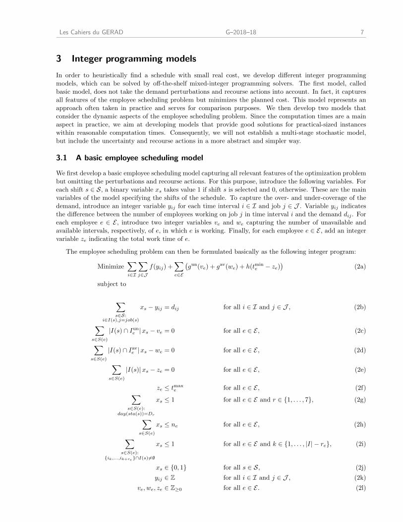
The employee scheduling problem can then be formulated basically as the following integer program:

Minimize∑i∈I

∑j∈J

f(yij) +∑e∈E

(gun(ve) + gav(we) + h(tmin

e − ze))

(2a)

subject to

∑s∈S:

i∈I(s),j=job(s)

xs − yij = dij for all i ∈ I and j ∈ J , (2b)

∑s∈S(e)

|I(s) ∩ Iune |xs − ve = 0 for all e ∈ E , (2c)

∑s∈S(e)

|I(s) ∩ Iave |xs − we = 0 for all e ∈ E , (2d)

∑s∈S(e)

|I(s)|xs − ze = 0 for all e ∈ E , (2e)

ze ≤ tmaxe for all e ∈ E , (2f)∑

s∈S(e):day(sta(s))=Dr

xs ≤ 1 for all e ∈ E and r ∈ {1, . . . , 7}, (2g)

∑s∈S(e)

xs ≤ ne for all e ∈ E , (2h)

∑s∈S(e):

{ik,...,ik+re}∩I(s)6=∅

xs ≤ 1 for all e ∈ E and k ∈ {1, . . . , |I| − re}, (2i)

xs ∈ {0, 1} for all s ∈ S, (2j)

yij ∈ Z for all i ∈ I and j ∈ J , (2k)

ve, we, ze ∈ Z≥0 for all e ∈ E . (2l)

8 G–2018–18 Les Cahiers du GERAD

The objective function (2a) minimizes the planned cost as defined in (1). Constraints (2b), (2c), (2d),

and (2e) link the (auxiliary) variables y, v, w, and z to the (main) variables x according to their meaning.

Constraints (2f) ensure that the employees’ maximum weekly work time limits are respected. Constraints (2g)

and (2h) limit the number of shifts assigned to an employee per day and week, respectively. Constraints (2i)

model the minimum rest period of re intervals between two shifts for each employee e by imposing that for

each set of re+1 consecutive time intervals, at most one selected shift of e must contain one of these intervals.

This ensures that, after the end of one shift of e, the next must start at least re time intervals later. Finally,

constraints (2j), (2k), and (2l) specify the domains of the decision variables.

The integer program (2) has a convex objective function. As all variables must take integer values, we

can assume –without loss of generality– that each of the convex functions f , gun, gav, and h is linear between

successive integers. As we have a minimization problem at hand, it is then easy to linearize the objective

function so that a mixed-integer linear program is obtained. The linearization step is carried out in detail in

the appendix.

3.2 A simple robust employee scheduling model

We now aim at including information about the possible demand perturbations and recourse actions to the

basic model (2). Consider the shifts that could reduce a demand under-coverage arising from a perturbation

when extending them. In the following simple robust employee scheduling model (or simple model for short),

the selection of these shifts, called extensible shifts, is favored by assigning a bonus term in the objective

function of (2). Consequently, a (near-) optimal solution of this model not only has a low planned cost but

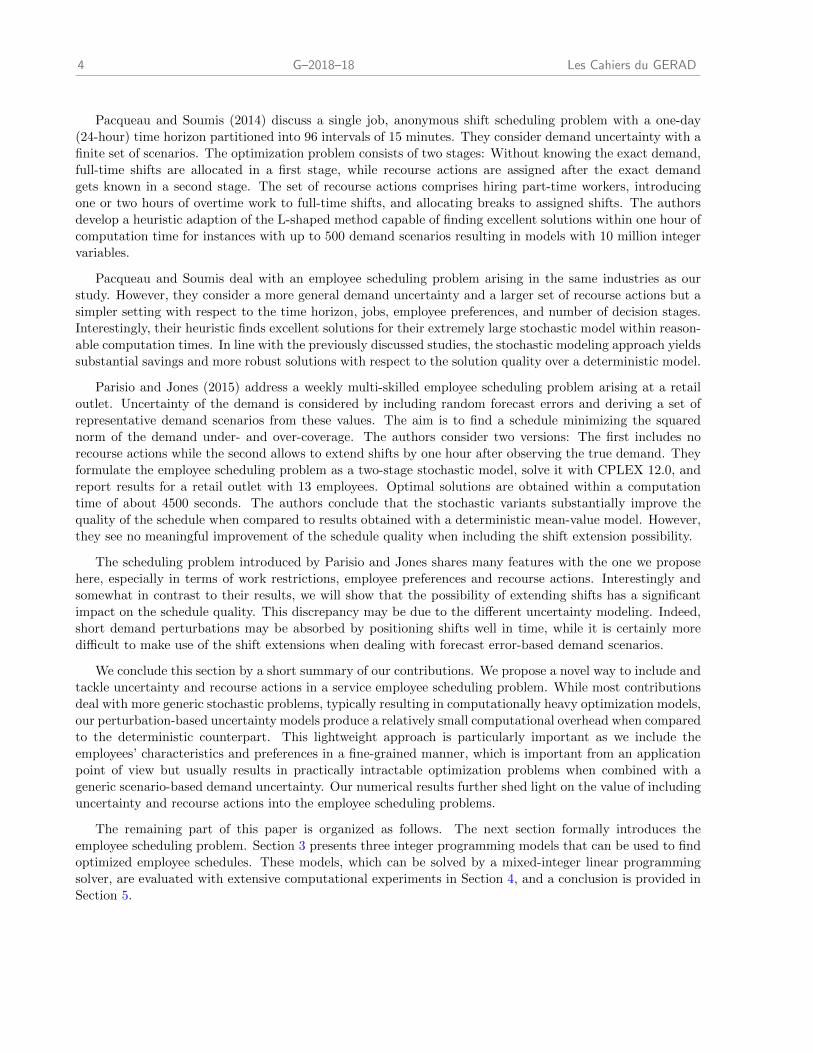
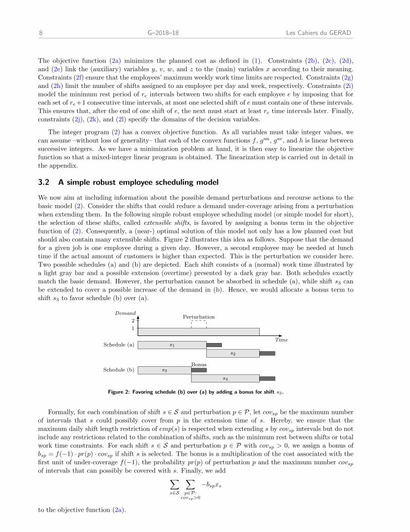
should also contain many extensible shifts. Figure 2 illustrates this idea as follows. Suppose that the demand

for a given job is one employee during a given day. However, a second employee may be needed at lunch

time if the actual amount of customers is higher than expected. This is the perturbation we consider here.

Two possible schedules (a) and (b) are depicted. Each shift consists of a (normal) work time illustrated by

a light gray bar and a possible extension (overtime) presented by a dark gray bar. Both schedules exactly

match the basic demand. However, the perturbation cannot be absorbed in schedule (a), while shift s3 can

be extended to cover a possible increase of the demand in (b). Hence, we would allocate a bonus term to

shift s3 to favor schedule (b) over (a).

Time

Demand

1

2Perturbation

Schedule (a) s1

s2

BonusSchedule (b) s3

s4

Figure 2: Favoring schedule (b) over (a) by adding a bonus for shift s3.

Formally, for each combination of shift s ∈ S and perturbation p ∈ P, let covsp be the maximum number

of intervals that s could possibly cover from p in the extension time of s. Hereby, we ensure that the

maximum daily shift length restriction of emp(s) is respected when extending s by covsp intervals but do not

include any restrictions related to the combination of shifts, such as the minimum rest between shifts or total

work time constraints. For each shift s ∈ S and perturbation p ∈ P with covsp > 0, we assign a bonus of

bsp = f(−1) · pr(p) · covsp if shift s is selected. The bonus is a multiplication of the cost associated with the

first unit of under-coverage f(−1), the probability pr(p) of perturbation p and the maximum number covspof intervals that can possibly be covered with s. Finally, we add∑

s∈S

∑p∈P:

covsp>0

−bspxs

to the objective function (2a).

Les Cahiers du GERAD G–2018–18 9

The primary advantage of this model is its simplicity: It is structurally (almost) equivalent to the basic

model. Hence, we suppose that finding a (near-) optimal solution does not take much more time in the

simple than in the basic model. But there are also various limitations. First of all, although there is only

one type of demand in practice, we separately deal with the basic and perturbation demands. Indeed, the

basic demand can be covered with the “normal” intervals of the shifts and the perturbation demand with the

overtime parts. Without this strict separation of the two types of demands with respect to their coverage, a

more complex modeling approach would be necessary in our view. A next limitation is related to neglecting

both the amount of additional employees needed if a perturbation materializes and the number of bonuses

attributed for each perturbation. Hence, the distribution of extensible shifts among the perturbations may

be suboptimal: The number of extensible shifts may be too high for some perturbations while being too low

for others. Furthermore, some shifts s with covsp > 0 may not be available to cover additional demand of p

as an extension of s can conflict with the rest period or maximum total work time constraints.

3.3 An advanced robust employee scheduling model

In a second attempt, we develop a model that better distributes the extensible shifts among the perturbations.

For this purpose, we adjust the basic model (2) as follows. Considering all perturbations together, we intro-

duce a potential demand dpotij for each interval i ∈ I and job j ∈ J , i.e., dpot

ij =∑

p∈P:i∈I(p),j=job(p) inc(p).

Note that at most one perturbation contributes to a potential demand dpotij as we assume that same-job

perturbations are non-overlapping in time. We aim at covering the potential demand by shift extensions of

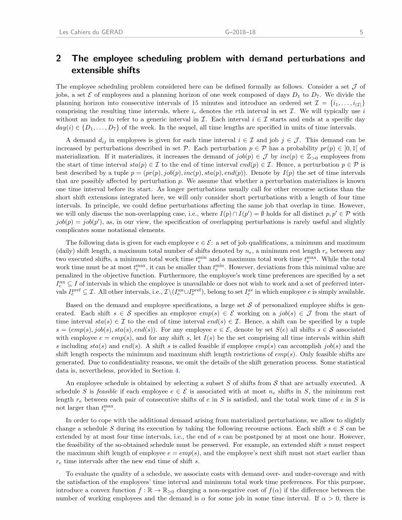
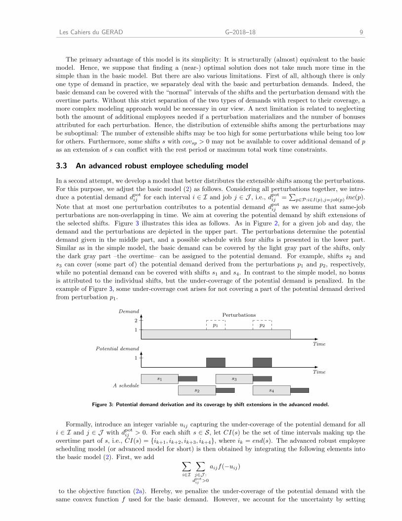
the selected shifts. Figure 3 illustrates this idea as follows. As in Figure 2, for a given job and day, the

demand and the perturbations are depicted in the upper part. The perturbations determine the potential

demand given in the middle part, and a possible schedule with four shifts is presented in the lower part.

Similar as in the simple model, the basic demand can be covered by the light gray part of the shifts, only

the dark gray part –the overtime– can be assigned to the potential demand. For example, shifts s2 and

s3 can cover (some part of) the potential demand derived from the perturbations p1 and p2, respectively,

while no potential demand can be covered with shifts s1 and s4. In contrast to the simple model, no bonus

is attributed to the individual shifts, but the under-coverage of the potential demand is penalized. In the

example of Figure 3, some under-coverage cost arises for not covering a part of the potential demand derived

from perturbation p1.

Time

Demand

1

2Perturbations

p1 p2

Time

Potential demand

1

A schedule

s1 s3

s2 s4

Figure 3: Potential demand derivation and its coverage by shift extensions in the advanced model.

Formally, introduce an integer variable uij capturing the under-coverage of the potential demand for all

i ∈ I and j ∈ J with dpotij > 0. For each shift s ∈ S, let CI(s) be the set of time intervals making up the

overtime part of s, i.e., CI(s) = {ik+1, ik+2, ik+3, ik+4}, where ik = end(s). The advanced robust employee

scheduling model (or advanced model for short) is then obtained by integrating the following elements into

the basic model (2). First, we add ∑i∈I

∑j∈J :

dpotij >0

aijf(−uij)

to the objective function (2a). Hereby, we penalize the under-coverage of the potential demand with the

same convex function f used for the basic demand. However, we account for the uncertainty by setting

10 G–2018–18 Les Cahiers du GERAD

parameter aij to the materialization probability of the perturbation that generated the potential demand for

job j in interval i. Then, we add the following potential demand coverage inequalities∑s∈S:

i∈CI(s),j=job(s)

xs + uij ≥ dpotij for all i ∈ I, j ∈ J with dpot

ij > 0, (3)

and, finally, we define the domain of the additional variables by adding the constraints

uij ∈ Z≥0 for all i ∈ I and j ∈ J .

This model captures the potential demand coverage in more detail than the simple model and it should

more accurately distribute the extensible shifts among the perturbations.

4 Computational experiments

To evaluate the performance of the developed employee scheduling models, we test them on a large set of

benchmark instances. The following computational environment is used for this purpose. The optimization

models are implemented in Java and solved with FICO Xpress-Optimizer version 7.4. The time limit is set

to one hour per optimization run measured as wall clock time. The computational work is performed on a

standard PC with an Intel Core i7-6700 3.4 GHz processor and 32 GB memory. The Xpress solver uses all

four cores in parallel.

We next describe the five data sets derived from real-world data of our industrial partner Kronos, then

explain the generation of the perturbations and the instances, and finally present and analyze the computa-

tional results.

4.1 Data sets

The five data sets, named RET1 to RET5, come from retail stores of different sectors and sizes. Each set

comprises the data for one week. We provide some of their characteristics in the upper part of Table 1 and

highlight the following. With respect to size, RET5 is quite small with only 17 employees, 2 jobs and a

total demand of 368 employee-hours, while RET1 to RET4 are substantially larger having about 25 to 47

employees, 2 to 7 jobs, and a demand between 618 to 1061 employee-hours. Each employee of RET1 and

RET2 can execute all the different jobs, while in the other data sets, employees are only qualified to perform

a subset of the jobs. The shift length and total work time restrictions usually depend on the type of contract.

Across all data sets, full-time workers must be assigned to about 8-hour long shifts and should work between

38 to 48 hours in total, while there is more flexibility with part-time workers. Finally, the minimum rest

length is about 8 to 10 hours, and the maximum number of shifts per employee is 5 in all data sets.

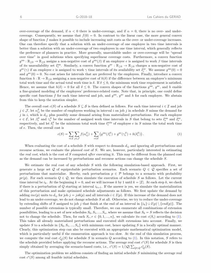
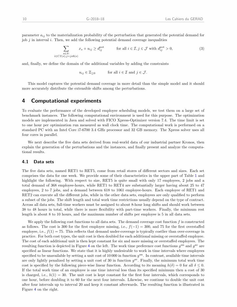
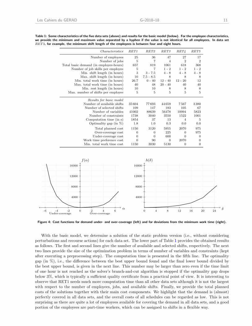
We apply the following cost functions to all data sets. The demand coverage cost function f is constructed

as follows. The cost is 300 for the first employee missing, i.e., f(−1) = 300, and 75 for the first overstaffed

employee, i.e., f(1) = 75. This reflects that demand under-coverage is typically costlier than over-coverage in

practice. For both cost types, the unit cost is then doubled for each additional missing or overstaffed employee.

The cost of each additional unit is then kept constant for six and more missing or overstaffed employees. The

resulting function is depicted in Figure 4 on the left. The work time preference cost functions gun and gav are

specified as linear functions. We state that it is highly undesirable to work in time intervals where employees

specified to be unavailable by setting a unit cost of 10 000 in function gun. In contrast, available time intervals

are only lightly penalized by setting a unit cost of 30 in function gav. Finally, the minimum total work time

cost is specified by the following piece-wise linear function. According to its meaning h(δ) = 0 for all δ ≤ 0.

If the total work time of an employee is one time interval less than its specified minimum then a cost of 30

is charged, i.e., h(1) = 30. The unit cost is kept constant for the first four intervals, which corresponds to

one hour, before doubling it to 60 for the next four intervals. Likewise, we continue to double the unit cost

after four intervals up to interval 20 and keep it constant afterwards. The resulting function is illustrated in

Figure 4 on the right.

Les Cahiers du GERAD G–2018–18 11

Table 1: Some characteristics of the five data sets (above) and results for the basic model (below). For the employee characteristics,we provide the minimum and maximum value separated by a hyphen if the value is not identical for all employees. In data setRET3, for example, the minimum shift length of the employees is between four and eight hours.

Characteristics RET1 RET2 RET3 RET4 RET5

Number of employees 25 36 47 27 17Number of jobs 5 7 4 2 2

Total basic demand (in employee-hours) 657 819 1061 618 368Number of job skills per employee 5 7 1 - 2 1 - 2 1 - 2

Min. shift length (in hours) 3 3 - 7.5 4 - 8 4 - 8 4 - 8Max. shift length (in hours) 10 7.5 - 8.5 8 8 8

Min. total work time (in hours) 26.7 0 - 40 12 - 40 12 - 20 12Max. total work time (in hours) 40 48 20 - 40 40 40

Min. rest length (in hours) 10 10 8 8 8Max. number of shifts per employee 5 5 5 5 5

Results for basic modelNumber of available shifts 35 604 77 693 44 659 7 567 3 380Number of selected shifts 109 147 183 105 67

Number of variables 41002 88639 56478 10994 5823Number of constraints 1738 3040 3550 1522 1001

Computation time (in s) 1854 37 13 4 5Optimality gap (in %) 1.8 1.0 0.3 0.0 0.0

Total planned cost 1150 3120 5955 2070 975Over-coverage cost 0 0 225 0 975

Under-coverage cost 0 0 600 0 0Work time preference cost 0 90 0 2070 0Min. total work time cost 1150 3030 5130 0 0

0 2 4 6-2-4-6

4000

8000

12000

16000

f(α)

α

Under-coverage Over-coverage0 4 8 12 16 20 24

4000

8000

12000

16000

h(δ)

δ

Figure 4: Cost functions for demand under- and over-coverage (left) and for deviations from the minimum work time (right).

With the basic model, we determine a solution of the static problem version (i.e., without considering

perturbations and recourse actions) for each data set. The lower part of Table 1 provides the obtained results

as follows. The first and second lines give the number of available and selected shifts, respectively. The next

two lines provide the size of the optimization problem in terms of number of variables and constraints (kept

after executing a preprocessing step). The computation time is presented in the fifth line. The optimality

gap (in %), i.e., the difference between the best upper bound found and the final lower bound divided by

the best upper bound, is given in the next line. This number may be larger than zero even if the time limit

of one hour is not reached as the solver’s branch-and-cut algorithm is stopped if the optimality gap drops

below 3%, which is typically a sufficient quality certificate from a practical point of view. It is interesting to

observe that RET1 needs much more computation time than all other data sets although it is not the largest

with respect to the number of employees, jobs, and available shifts. Finally, we provide the total planned

costs of the solutions together with their main cost components. We highlight that the demand is (almost)

perfectly covered in all data sets, and the overall costs of all schedules can be regarded as low. This is not

surprising as there are quite a lot of employees available for covering the demand in all data sets, and a good

portion of the employees are part-time workers, which can be assigned to shifts in a flexible way.

12 G–2018–18 Les Cahiers du GERAD

4.2 Generation of perturbations, scenarios, instances, and additional shifts

As the data sets we obtained contain no information about possible perturbations, we generated them as

follows. For each data set, we independently compute perturbations for each job and day. For a given job

and day, we first calculate the average demand avg per interval over the period ranging from first to the

last interval with a positive demand on this day. Depending on this average demand, we generate zero to

four perturbations. Specifically, the number of perturbations is set to min(4, davg − 1e). The second line in

Table 2 presents the resulting total number of perturbations per data set. It can be seen that this number

is about 22 to 33 for data sets RET1 to RET4, while data set RET5 only contains 10 perturbations. The

length of each perturbation is four time intervals, hence one hour, which reflect our aim to introduce short

perturbations. We randomly place the perturbations in time ensuring that same-job perturbations do not

overlap and no perturbation starts earlier than four hours after the first positive demand in employees for the

given job and day. There are two reasons for this rule. First, perturbations are typically less likely to occur

in the morning, and second, as the minimum shift length is usually at least about four hours, independent of

the optimization model, no shift can be extended to cover perturbations in the early morning. Motivated by

practical experience, for any perturbation, the increase in the number of employees is somewhat proportional

to the demand affected by the perturbation. More precisely, if the minimum basic demand affected by the

perturbation is at most 4, we assign an increase of 1 employee to the perturbation, if this demand is between 5

and 8, then we randomly pick an increase of 1 or 2, and if it is larger than 8, we randomly choose between

1, 2, and 3.

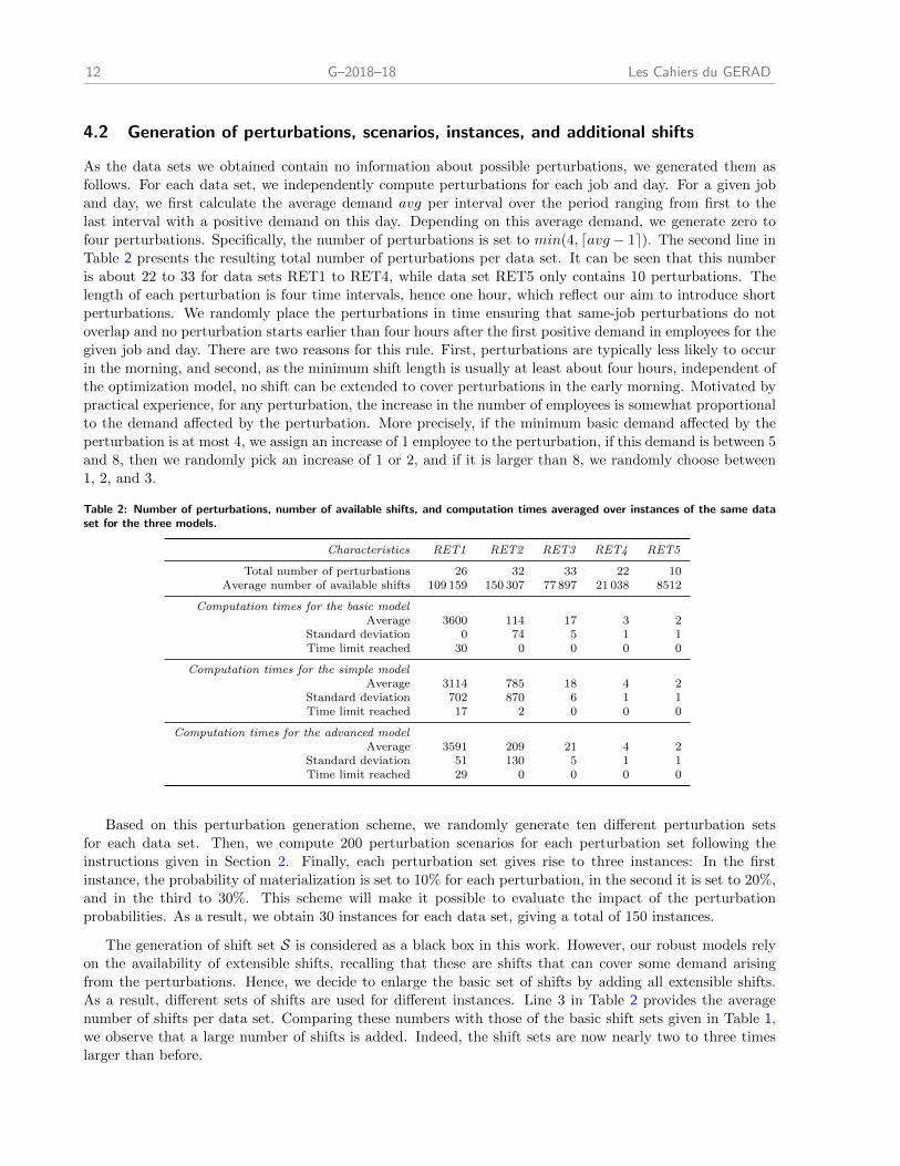
Table 2: Number of perturbations, number of available shifts, and computation times averaged over instances of the same dataset for the three models.

Characteristics RET1 RET2 RET3 RET4 RET5

Total number of perturbations 26 32 33 22 10Average number of available shifts 109 159 150 307 77 897 21 038 8512

Computation times for the basic modelAverage 3600 114 17 3 2

Standard deviation 0 74 5 1 1Time limit reached 30 0 0 0 0

Computation times for the simple modelAverage 3114 785 18 4 2

Standard deviation 702 870 6 1 1Time limit reached 17 2 0 0 0

Computation times for the advanced modelAverage 3591 209 21 4 2

Standard deviation 51 130 5 1 1Time limit reached 29 0 0 0 0

Based on this perturbation generation scheme, we randomly generate ten different perturbation sets

for each data set. Then, we compute 200 perturbation scenarios for each perturbation set following the

instructions given in Section 2. Finally, each perturbation set gives rise to three instances: In the first

instance, the probability of materialization is set to 10% for each perturbation, in the second it is set to 20%,

and in the third to 30%. This scheme will make it possible to evaluate the impact of the perturbation

probabilities. As a result, we obtain 30 instances for each data set, giving a total of 150 instances.

The generation of shift set S is considered as a black box in this work. However, our robust models rely

on the availability of extensible shifts, recalling that these are shifts that can cover some demand arising

from the perturbations. Hence, we decide to enlarge the basic set of shifts by adding all extensible shifts.

As a result, different sets of shifts are used for different instances. Line 3 in Table 2 provides the average

number of shifts per data set. Comparing these numbers with those of the basic shift sets given in Table 1,

we observe that a large number of shifts is added. Indeed, the shift sets are now nearly two to three times

larger than before.

Les Cahiers du GERAD G–2018–18 13

4.3 Computational tests and results

We execute one optimization run for each combination of instance and model version (i.e., basic, simple, and

advanced), giving a total of 150 · 3 = 450 runs. For each obtained solution, we then compute its real cost for

its 200 scenarios using the simulation-based approach described in Section 2. This gives 200 results for each

combination of instance and model version. Note that we decided to run the basic model for each instance

with the enlarged shift set as it may benefit from the additional shifts when compared with its results ob-

tained with the smaller shift sets (see Table 1). In our view, this setting enables a fair comparison of the three

methods, and the basic model’s results obtained with the smaller shift sets serve for comparison purposes.

We first discuss the computation times, which are given for each data set individually in Table 2. Looking

at the average computation times (of the 30 runs, one per instance), we observe that the three models are

solved within a few seconds for RET3, RET4, and RET5 instances, but it takes considerably more time to

solve RET1 and RET2 instances. This can be explained in good part by their shift set size, which is typically

a main driver of the computational effort in this type of scheduling models. Indeed, when looking at the

computation times of the basic model obtained with the basic shift sets, see Table 1, one can observe that

the solution times for RET1 and RET2 instances substantially increased when enlarging the shift sets. When

comparing the three models with each other, it seems impossible to rank them with respect to computation

times: There is no model significantly solved faster across the different instances. Establishing a ranking is

also impeded by the high variance of the computation times. Finally, we observe that a considerable amount

of runs of RET1 and a few of RET2 instances did not terminate before the time limit was reached.

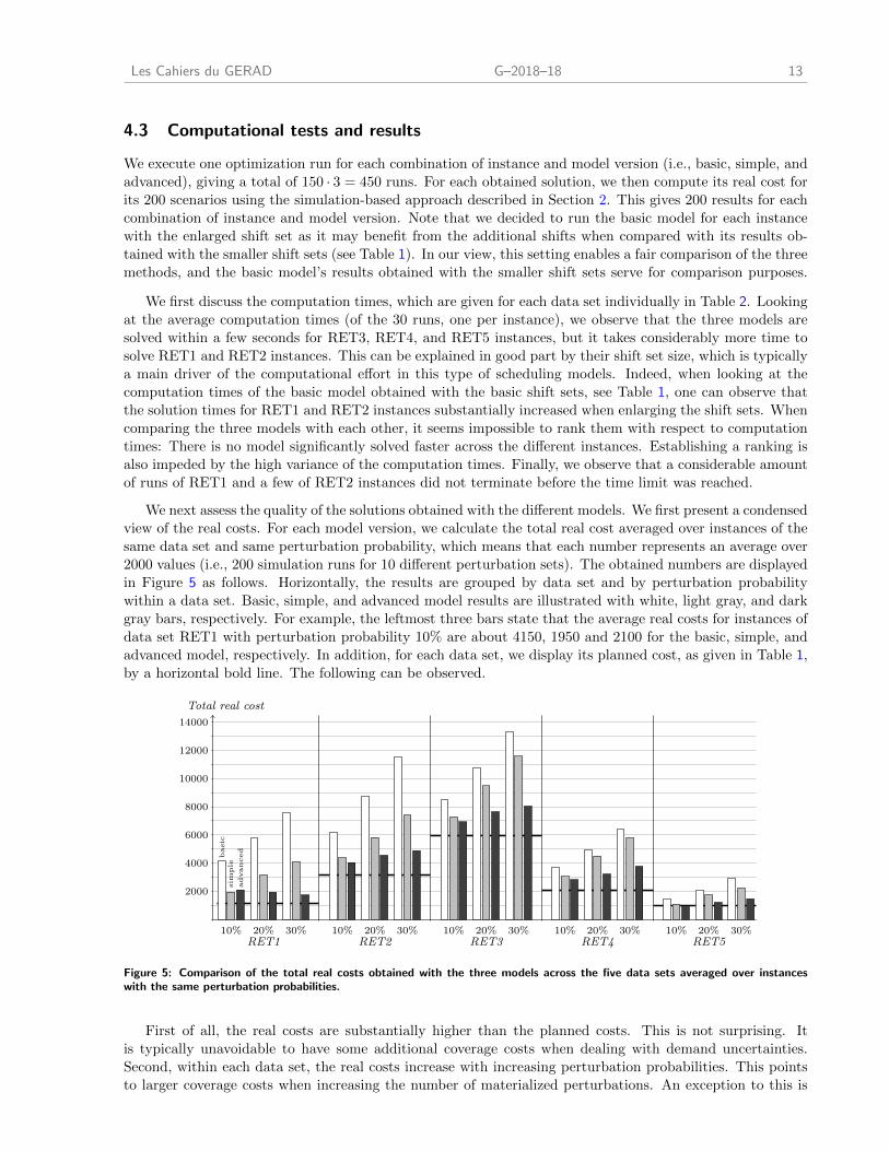
We next assess the quality of the solutions obtained with the different models. We first present a condensed

view of the real costs. For each model version, we calculate the total real cost averaged over instances of the

same data set and same perturbation probability, which means that each number represents an average over

2000 values (i.e., 200 simulation runs for 10 different perturbation sets). The obtained numbers are displayed

in Figure 5 as follows. Horizontally, the results are grouped by data set and by perturbation probability

within a data set. Basic, simple, and advanced model results are illustrated with white, light gray, and dark

gray bars, respectively. For example, the leftmost three bars state that the average real costs for instances of

data set RET1 with perturbation probability 10% are about 4150, 1950 and 2100 for the basic, simple, and

advanced model, respectively. In addition, for each data set, we display its planned cost, as given in Table 1,

by a horizontal bold line. The following can be observed.

2000

4000

6000

8000

10000

12000

14000

Total real cost

RET110% 20% 30%

basic

sim

ple

advanced

RET210% 20% 30%

RET310% 20% 30%

RET410% 20% 30%

RET510% 20% 30%

Figure 5: Comparison of the total real costs obtained with the three models across the five data sets averaged over instanceswith the same perturbation probabilities.

First of all, the real costs are substantially higher than the planned costs. This is not surprising. It

is typically unavoidable to have some additional coverage costs when dealing with demand uncertainties.

Second, within each data set, the real costs increase with increasing perturbation probabilities. This points

to larger coverage costs when increasing the number of materialized perturbations. An exception to this is

14 G–2018–18 Les Cahiers du GERAD

provided by the advanced model for data set RET1, for which the average cost decreases with increasing

perturbation probability. This can be attributed to the heuristic nature of the optimization approach, and

to the additional work generated by the perturbations, which may decrease the minimum work time costs.

Third, as expected, both robust models produce substantially better results than the basic model. And

fourth, the advanced model gives better results than the simple model.

In order to compare the results of the three models in detail, we additionally perform the following

analysis. As described in Section 2, each schedule is evaluated using the set of scenarios, obtaining the real

cost (and cost components) for each of the 200 scenarios. In order to compare the results of the simple with

the basic model, we now calculate the difference in the total real cost and in the number of under- and over-

covered employee-hours between the solutions of the two models for each instance and scenario combination.

We then do the same calculations for comparing the advanced with the basic model and the advanced with

the simple model.

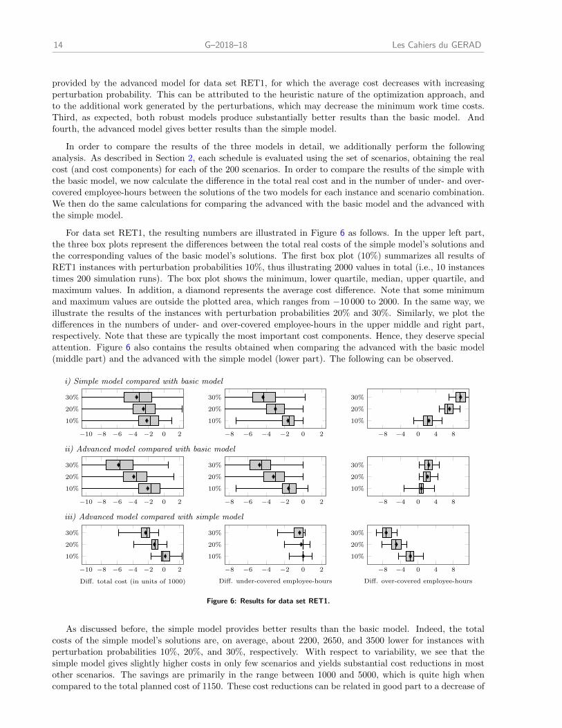
For data set RET1, the resulting numbers are illustrated in Figure 6 as follows. In the upper left part,

the three box plots represent the differences between the total real costs of the simple model’s solutions and

the corresponding values of the basic model’s solutions. The first box plot (10%) summarizes all results of

RET1 instances with perturbation probabilities 10%, thus illustrating 2000 values in total (i.e., 10 instances

times 200 simulation runs). The box plot shows the minimum, lower quartile, median, upper quartile, and

maximum values. In addition, a diamond represents the average cost difference. Note that some minimum

and maximum values are outside the plotted area, which ranges from −10 000 to 2000. In the same way, we

illustrate the results of the instances with perturbation probabilities 20% and 30%. Similarly, we plot the

differences in the numbers of under- and over-covered employee-hours in the upper middle and right part,

respectively. Note that these are typically the most important cost components. Hence, they deserve special

attention. Figure 6 also contains the results obtained when comparing the advanced with the basic model

(middle part) and the advanced with the simple model (lower part). The following can be observed.

i) Simple model compared with basic model

−10 −8 −6 −4 −2 0 2

10%

20%

30%

−8 −6 −4 −2 0 2

10%

20%

30%

−8 −4 0 4 8

10%

20%

30%

ii) Advanced model compared with basic model

−10 −8 −6 −4 −2 0 2

10%

20%

30%

−8 −6 −4 −2 0 2

10%

20%

30%

−8 −4 0 4 8

10%

20%

30%

iii) Advanced model compared with simple model

−10 −8 −6 −4 −2 0 2

10%

20%

30%

Diff. total cost (in units of 1000)

−8 −6 −4 −2 0 2

10%

20%

30%

Diff. under-covered employee-hours

−8 −4 0 4 8

10%

20%

30%

Diff. over-covered employee-hours

Figure 6: Results for data set RET1.

As discussed before, the simple model provides better results than the basic model. Indeed, the total

costs of the simple model’s solutions are, on average, about 2200, 2650, and 3500 lower for instances with

perturbation probabilities 10%, 20%, and 30%, respectively. With respect to variability, we see that the

simple model gives slightly higher costs in only few scenarios and yields substantial cost reductions in most

other scenarios. The savings are primarily in the range between 1000 and 5000, which is quite high when

compared to the total planned cost of 1150. These cost reductions can be related in good part to a decrease of

Les Cahiers du GERAD G–2018–18 15

understaffing. As expected, the basic demand is typically covered well by both solutions but the simple model

better handles the perturbations as confirmed by the differences in under-covered employee-hours. Indeed,

the simple model typically reduces the number of under-covered employee-hours by two to five. The simple

model is especially at an advantage when many perturbations materialize. This can be seen, for example, by

higher cost savings with larger perturbation probabilities. However, it can also be seen that the simple model

substantially increases overstaffing when compared to the basic model, see upper right part in Figure 6.

Similar conclusions can be found when comparing the advanced with the basic model (see middle part of

Figure 6). Indeed, the advanced model outputs schedules with lower costs and better coverage of the actual

demand. The average savings are about 2000, 3850, and 5850 for instances with perturbation probabilities

10%, 20%, and 30%, respectively. These improvements are achieved while slightly increasing the over-coverage

costs. However, as seen when comparing the advanced with the simple model (see lower part of Figure 6),

the advanced model uses significantly less overstaffing than the simple model while still slightly reducing the

under-coverage costs. Consequently, the advanced model has an edge over the simple model, especially with

higher perturbation probabilities. Indeed, we observe that both models have a similar quality in instances

with perturbation probability 10%, with a slight edge for the simple model, but the advanced model performs

considerably better for instances with perturbation probability 20% and 30%.

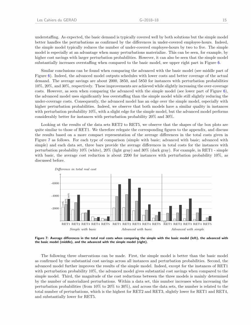
Looking at the results of the data sets RET2 to RET5, we observe that the shapes of the box plots are

quite similar to those of RET1. We therefore relegate the corresponding figures to the appendix, and discuss

the results based on a more compact representation of the average differences in the total costs given in

Figure 7 as follows. For each type of comparison (simple with basic; advanced with basic; advanced with

simple) and each data set, three bars provide the average differences in total costs for the instances with

perturbation probability 10% (white), 20% (light gray) and 30% (dark gray). For example, in RET1 - simple

with basic, the average cost reduction is about 2200 for instances with perturbation probability 10%, as

discussed before.

Simple with basic

-2000

-4000

-6000

Difference in total real cost

RET1 RET2 RET3 RET4 RET5

10% 20%

30%

Advanced with basic

RET1 RET2 RET3 RET4 RET5

Advanced with simple

RET1 RET2 RET3 RET4 RET5

Figure 7: Average differences in the total real costs when comparing the simple with the basic model (left), the advanced withthe basic model (middle), and the advanced with the simple model (right).

The following three observations can be made. First, the simple model is better than the basic model

as confirmed by the substantial cost savings across all instances and perturbation probabilities. Second, the

advanced model further improves the results of the simple model. Indeed, except for the instances of RET1

with perturbation probability 10%, the advanced model gives substantial cost savings when compared to the

simple model. Third, the magnitude of the cost reductions between the three models is mainly determined

by the number of materialized perturbations. Within a data set, this number increases when increasing the

perturbation probabilities (from 10% to 20% to 30%), and across the data sets, the number is related to the

total number of perturbations, which is the highest for RET2 and RET3, slightly lower for RET1 and RET4,

and substantially lower for RET5.

16 G–2018–18 Les Cahiers du GERAD

Altogether, we conclude that the simple and advanced models provide robust solutions within a reasonable

computation time for the discussed employee scheduling problem, and the advanced model has an edge over

the simple model in terms of solution quality. This advantage is mainly due to a better control of overstaffing.

5 Conclusion

This article discussed an employee scheduling problem including short demand perturbations and extensible

shifts. We proposed two integer programming models for establishing an initial schedule that is robust with

respect to the considered uncertainty and recourse actions. In the first model, called simple model, a bonus

term is assigned to shifts that can cover some perturbation demand when postponing the shift’s end time,

while in the second model, called advanced model, a potential demand curve is derived from the perturbations

and its coverage with shift extensions is forced by penalizing the under-coverage of the potential demand. We

executed extensive computational tests on retail shop instances. A detailed analysis of the obtained results

revealed that the two robust models enable to significantly improve the schedule quality when compared

with a basic, non-robust model. When comparing the results of the two robust models with each other, we

observe that the advanced model has an edge over the simple model with respect to the solution quality.

Altogether, this study underpins the value of including uncertainty information and recourse actions in the

initial scheduling activity.

This article suggests various avenues for interesting further research. As remarked by Parisio and Jones

(2015), the schedule quality heavily depends on the accuracy of the inputs, which includes problem modeling

and data estimation aspects in our view. With respect to demand uncertainty, one may study how to best

represent it. Short perturbations may be a good means to model, for example, uncertainty about peak

hour demand, while more generic demand scenarios might be better in other cases. Hereby, more attention

should be paid to developing stochastic models that are including the dynamic aspects of the employee

scheduling process and that are “solvable” from a practical perspective. Other important aspects are related

to the recourse actions. One may include more re-adjustment possibilities than shift extensions, such as

small changes of the shifts’ start and end times, re-assignments of the jobs, creation of additional shifts, and

canceling of shifts. However, one should also care about the downside effects of schedule updates such as

employee dissatisfaction. Finally, the optimization approaches discussed in this paper assume that a set of

shifts is given. Obviously, the shift generation process is itself not simple and deserves special attention. The

set of shifts should be generated with the structure of the optimization process in mind. In this paper, for

example, it was crucial to generate extensible shifts. However, a large number of shifts was obtained as we

included all of the extensible ones. This negatively affected the computation times. Further research maydiscuss the shift generation process for robust employee scheduling problems in more detail.

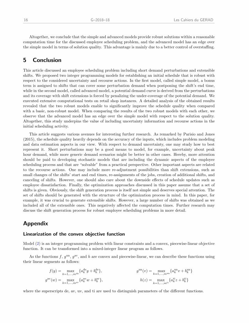
Appendix

Linearization of the convex objective function

Model (2) is an integer programming problem with linear constraints and a convex, piecewise-linear objective

function. It can be transformed into a mixed-integer linear program as follows.

As the functions f , gun, gav, and h are convex and piecewise-linear, we can describe these functions using

their linear segments as follows:

f(y) = maxk=1,...,mde

{adek y + bde

k }, gun(v) = maxk=1,...,mun

{aunk v + bun

k }

gav(w) = maxk=1,...,mav

{aavk w + bav

k }, h(z) = maxk=1,...,mti

{atik z + btik }

where the superscripts de, av, uv, and ti are used to distinguish parameters of the different functions.

Les Cahiers du GERAD G–2018–18 17

Introduce a continuous variable udeij for all i ∈ I, j ∈ J , and three continuous variables uun

e , uave , and uti

e

for all e ∈ E . Replace objective (2a) by

Minimize∑i∈I

∑i∈I

udeij +

∑e∈E

(uune + uav

e + utie

),

and add the following linear constraints to model (2):

udeij −

(adek yij + bde

k

)≥ 0 for all i ∈ I, j ∈ J , and k ∈ {1, . . . ,mde},

uune − (aun

k ve + bunk ) ≥ 0 for all e ∈ E and k ∈ {1, . . . ,mun},

uave − (aav

k we + bavk ) ≥ 0 for all e ∈ E and k ∈ {1, . . . ,mav},

utie −

(atik ze + btik

)≥ 0 for all e ∈ E and k ∈ {1, . . . ,mti}.

The optimization model obtained with this standard transformation is a mixed-integer linear program.

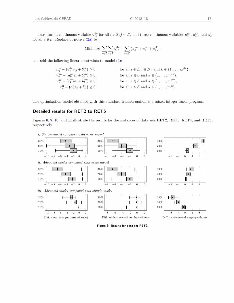
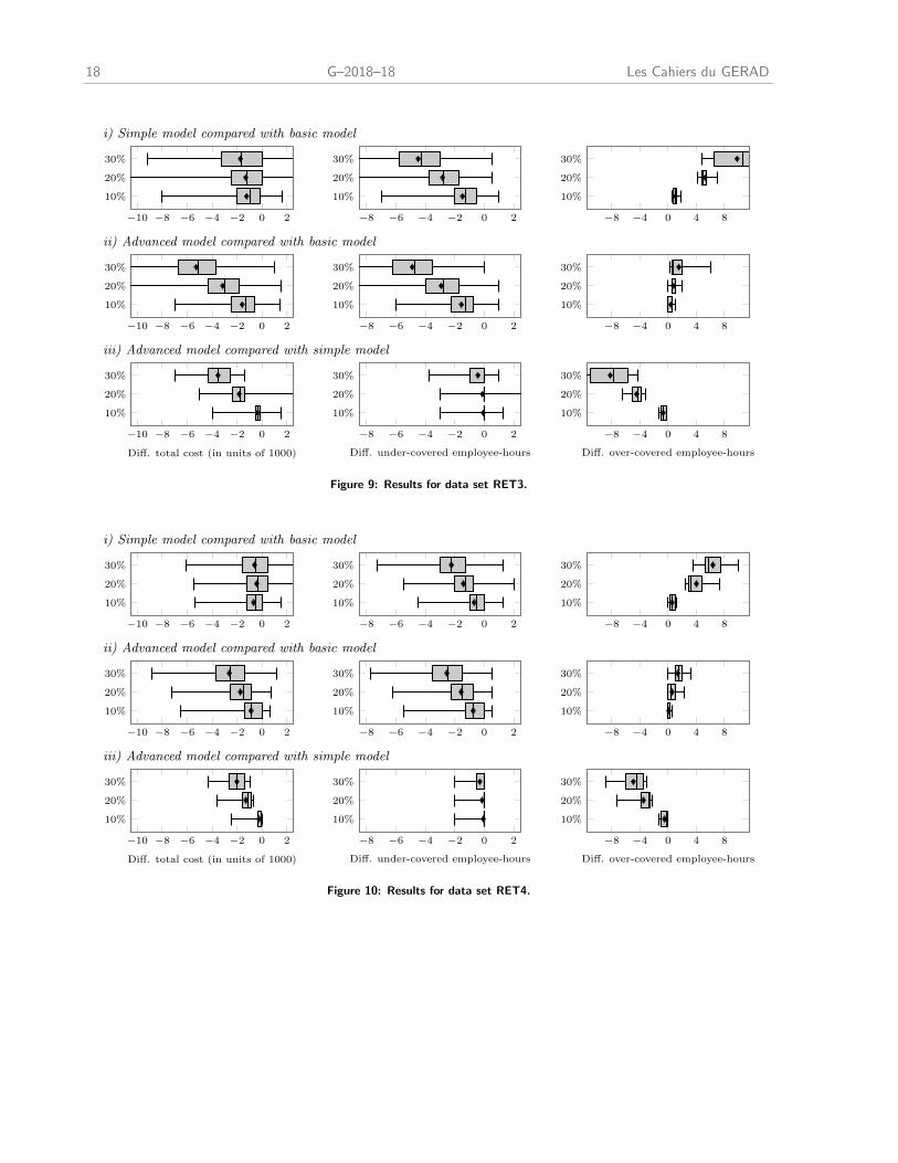
Detailed results for RET2 to RET5

Figures 8, 9, 10, and 11 illustrate the results for the instances of data sets RET2, RET3, RET4, and RET5,

respectively.

i) Simple model compared with basic model

−10 −8 −6 −4 −2 0 2

10%

20%

30%

−8 −6 −4 −2 0 2

10%

20%

30%

−8 −4 0 4 8

10%

20%

30%

ii) Advanced model compared with basic model

−10 −8 −6 −4 −2 0 2

10%

20%

30%

−8 −6 −4 −2 0 2

10%

20%

30%

−8 −4 0 4 8

10%

20%

30%

iii) Advanced model compared with simple model

−10 −8 −6 −4 −2 0 2

10%

20%

30%

Diff. total cost (in units of 1000)

−8 −6 −4 −2 0 2

10%

20%

30%

Diff. under-covered employee-hours

−8 −4 0 4 8

10%

20%

30%

Diff. over-covered employee-hours

Figure 8: Results for data set RET2.

18 G–2018–18 Les Cahiers du GERAD

i) Simple model compared with basic model

−10 −8 −6 −4 −2 0 2

10%

20%

30%

−8 −6 −4 −2 0 2

10%

20%

30%

−8 −4 0 4 8

10%

20%

30%

ii) Advanced model compared with basic model

−10 −8 −6 −4 −2 0 2

10%

20%

30%

−8 −6 −4 −2 0 2

10%

20%

30%

−8 −4 0 4 8

10%

20%

30%

iii) Advanced model compared with simple model

−10 −8 −6 −4 −2 0 2

10%

20%

30%

Diff. total cost (in units of 1000)

−8 −6 −4 −2 0 2

10%

20%

30%

Diff. under-covered employee-hours

−8 −4 0 4 8

10%

20%

30%

Diff. over-covered employee-hours

Figure 9: Results for data set RET3.

i) Simple model compared with basic model

−10 −8 −6 −4 −2 0 2

10%

20%

30%

−8 −6 −4 −2 0 2

10%

20%

30%

−8 −4 0 4 8

10%

20%

30%

ii) Advanced model compared with basic model

−10 −8 −6 −4 −2 0 2

10%

20%

30%

−8 −6 −4 −2 0 2

10%

20%

30%

−8 −4 0 4 8

10%

20%

30%

iii) Advanced model compared with simple model

−10 −8 −6 −4 −2 0 2

10%

20%

30%

Diff. total cost (in units of 1000)

−8 −6 −4 −2 0 2

10%

20%

30%

Diff. under-covered employee-hours

−8 −4 0 4 8

10%

20%

30%

Diff. over-covered employee-hours

Figure 10: Results for data set RET4.

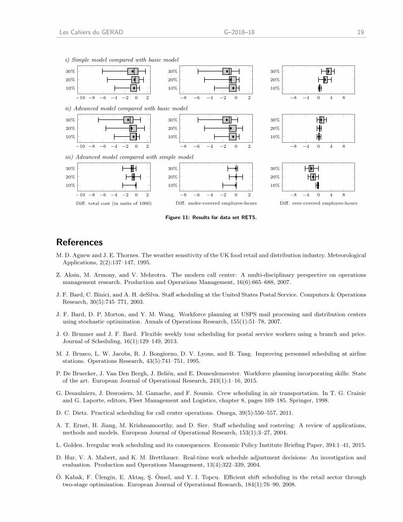
Les Cahiers du GERAD G–2018–18 19

i) Simple model compared with basic model

−10 −8 −6 −4 −2 0 2

10%

20%

30%

−8 −6 −4 −2 0 2

10%

20%

30%

−8 −4 0 4 8

10%

20%

30%

ii) Advanced model compared with basic model

−10 −8 −6 −4 −2 0 2

10%

20%

30%

−8 −6 −4 −2 0 2

10%

20%

30%

−8 −4 0 4 8

10%

20%

30%

iii) Advanced model compared with simple model

−10 −8 −6 −4 −2 0 2

10%

20%

30%

Diff. total cost (in units of 1000)

−8 −6 −4 −2 0 2

10%

20%

30%

Diff. under-covered employee-hours

−8 −4 0 4 8

10%

20%

30%

Diff. over-covered employee-hours

Figure 11: Results for data set RET5.

ReferencesM. D. Agnew and J. E. Thornes. The weather sensitivity of the UK food retail and distribution industry. Meteorological

Applications, 2(2):137–147, 1995.

Z. Aksin, M. Armony, and V. Mehrotra. The modern call center: A multi-disciplinary perspective on operationsmanagement research. Production and Operations Management, 16(6):665–688, 2007.

J. F. Bard, C. Binici, and A. H. deSilva. Staff scheduling at the United States Postal Service. Computers & OperationsResearch, 30(5):745–771, 2003.

J. F. Bard, D. P. Morton, and Y. M. Wang. Workforce planning at USPS mail processing and distribution centersusing stochastic optimization. Annals of Operations Research, 155(1):51–78, 2007.

J. O. Brunner and J. F. Bard. Flexible weekly tour scheduling for postal service workers using a branch and price.Journal of Scheduling, 16(1):129–149, 2013.

M. J. Brusco, L. W. Jacobs, R. J. Bongiorno, D. V. Lyons, and B. Tang. Improving personnel scheduling at airlinestations. Operations Research, 43(5):741–751, 1995.

P. De Bruecker, J. Van Den Bergh, J. Belien, and E. Demeulemeester. Workforce planning incorporating skills: Stateof the art. European Journal of Operational Research, 243(1):1–16, 2015.

G. Desaulniers, J. Desrosiers, M. Gamache, and F. Soumis. Crew scheduling in air transportation. In T. G. Crainicand G. Laporte, editors, Fleet Management and Logistics, chapter 8, pages 169–185. Springer, 1998.

D. C. Dietz. Practical scheduling for call center operations. Omega, 39(5):550–557, 2011.

A. T. Ernst, H. Jiang, M. Krishnamoorthy, and D. Sier. Staff scheduling and rostering: A review of applications,methods and models. European Journal of Operational Research, 153(1):3–27, 2004.

L. Golden. Irregular work scheduling and its consequences. Economic Policy Institute Briefing Paper, 394:1–41, 2015.

D. Hur, V. A. Mabert, and K. M. Bretthauer. Real-time work schedule adjustment decisions: An investigation andevaluation. Production and Operations Management, 13(4):322–339, 2004.

O. Kabak, F. Ulengin, E. Aktas, S. Onsel, and Y. I. Topcu. Efficient shift scheduling in the retail sector throughtwo-stage optimization. European Journal of Operational Research, 184(1):76–90, 2008.

20 G–2018–18 Les Cahiers du GERAD

A. Kasirzadeh, M. Saddoune, and F. Soumis. Airline crew scheduling: Models, algorithms, and data sets. EUROJournal on Transportation and Logistics, 6(2):111–137, 2017.

K. Kim and S. Mehrotra. A two-stage stochastic integer programming approach to integrated staffing and schedulingwith application to nurse management. Operations Research, 63(6):1431–1451, 2015.

S. Lam, M. Vandenbosch, and M. Pearce. Retail sales force scheduling based on store traffic forecasting. Journal ofRetailing, 74(1):61–88, 1998.

A. Legrain, H. Bouarab, and N. Lahrichi. The nurse scheduling problem in real-life. Journal of Medical Systems,39(1):160, 2015.

R. R. Love Jr. and J. M. Hoey. Management science improves fast-food operations. Interfaces, 20(2):21–29, 1990.

V. Mani, S. Kesavan, and J. M. Swaminathan. Estimating the impact of understaffing on sales and profitability inretail stores. Production and Operations Management, 24(2):201–218, 2015.

V. Mehrotra, O. Ozluk, and R. Saltzman. Intelligent procedures for intra-day updating of call center agent schedules.Production and Operations Management, 19(3):353–367, 2010.

NYT Editorial Board. Schedules that don’t work. The New York Times, CLXIV(56,976):A22, 2015. URL https:

//nyti.ms/2psHvIt.

R. Pacqueau and F. Soumis. Shift scheduling under stochastic demand. Technical Report G-2014-46, Les Cahiers duGERAD, HEC Montreal, Canada, 2014.

A. Parisio and C. N. Jones. A two-stage stochastic programming approach to employee scheduling in retail outletswith uncertain demand. Omega, 53:97–103, 2015.

O. Perdikaki, S. Kesavan, and J. M. Swaminathan. Effect of traffic on sales and conversion rates of retail stores.Manufacturing & Service Operations Management, 14(1):145–162, 2012.

M. I. Restrepo, B. Gendron, and L.-M. Rousseau. A two-stage stochastic programming approach for multi-activitytour scheduling. European Journal of Operational Research, 262(2):620–635, 2017.

H. Shen and J. Z. Huang. Interday forecasting and intraday updating of call center arrivals. Manufacturing & ServiceOperations Management, 10(3):391–410, 2008.

J. Van Den Bergh, J. Belien, P. De Bruecker, E. Demeulemeester, and L. De Boeck. Personnel scheduling: A literaturereview. European Journal of Operational Research, 226(3):367–385, 2013.

P. D. Wright and S. Mahar. Centralized nurse scheduling to simultaneously improve schedule cost and nurse satisfac-tion. Omega, 41(6):1042–1052, 2013.