Embed Size (px)
Citation preview


Sistemas embebidos: Estado actual con visión al futuro Editado por Marco Antonio Aceves Fernández, José Emilio Vargas Soto Carlos Alberto Ramos Arreguín y Santiago Miguel Fernández Fraga
Publicado por:
Asociación Mexicana de Mecatrónica A.C.
Asociación Mexicana de Software Embebido A.C.
© Los editores
Sistemas embebidos: Estado actual con visión al futuro, es un libro digital autorizado por el Instituto Nacional de Derechos de Autor bajo el número de radicación 311011 a la Asociación Mexicana de Mecatrónica A.C., Fonología 116, Colonia Tecnológico C.P. 76158 Querétaro, Qro. México. Tel. (01-442) 224-0257, www.mecamex.net, las opiniones y la información que se muestran en los capítulos del libro son exclusivas de los autores y no representan la postura de la Asociación Mexicana Mecatrónica A.C. Fecha de la última modificación 10 de marzo 2017. Esta obra es una publicación de acceso abierto, distribuido bajo los términos de la Asociación Mexicana de Mecatrónica A.C., la cual permite el uso, distribución y reproducción sin restricciones por cualquier medio, siempre y cuando los trabajos estén apropiadamente citados, respetando la autoría de las personas que realizaron los capítulos.
Impreso y hecho en México
Primera edición, 17 de marzo 2017
ISBN 978-607-9394-08-0
Sistemas embebidos: Estado actual con visión al futuro
ISBN 978-607-9394-08-0, Asociación Mexicana de Mecatrónica A.C.
1
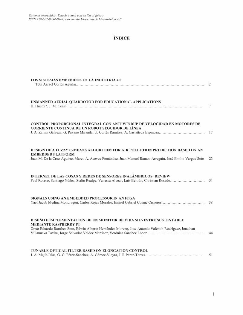
ÍNDICE
LOS SISTEMAS EMBEBIDOS EN LA INDUSTRIA 4.0 Teth Azrael Cortés Aguilar.………………………………………………………………………………………… 2
UNMANNED AERIAL QUADROTOR FOR EDUCATIONAL APPLICATIONS
H. Huerta*, J. M. Ceñal ………………………...……………………………………………………………………. 7
CONTROL PROPORCIONAL INTEGRAL CON ANTI WINDUP DE VELOCIDAD EN MOTORES DE CORRIENTE CONTINUA DE UN ROBOT SEGUIDOR DE LÍNEA
J. A. Zanini Gálveza, G. Payano Miranda, U. Cortés Ramírez, A. Castañeda Espinoza………………………………. 17
DESIGN OF A FUZZY C-MEANS ALGORITHM FOR AIR POLLUTION PREDICTION BASED ON AN EMBEDDED PLATFORM
Juan M. De la Cruz-Aguirre, Marco A. Aceves-Fernández, Juan Manuel Ramos-Arreguín, José Emilio Vargas-Soto 23
INTERNET DE LAS COSAS Y REDES DE SENSORES INALÁMBRICOS: REVIEW
Paul Rosero, Santiago Núñez, Stalin Realpe, Vanessa Alvear, Luis Beltrán, Christian Rosado………………………. 31
SIGNALS USING AN EMBEDDED PROCESSOR IN AN FPGA
Yael Jacob Medina Mondragón, Carlos Rojas Morales, Ismael Gabriel Cosme Cisneros…………………………….. 38
DISEÑO E IMPLEMENTACIÓN DE UN MONITOR DE VIDA SILVESTRE SUSTENTABLE MEDIANTE RASPBERRY PI
Omar Eduardo Ramírez Soto, Edwin Alberto Hernández Moreno, José Antonio Valentín Rodríguez, Jonathan Villanueva Tavira, Jorge Salvador Valdez Martínez, Verónica Sánchez López………………………………….……
44
TUNABLE OPTICAL FILTER BASED ON ELONGATION CONTROL
J. A. Mejía-Islas, G. G. Pérez-Sánchez, A. Gómez-Vieyra, J. R Pérez-Torres………………………………….…… 51
Sistemas embebidos: Estado actual con visión al futuro
ISBN 978-607-9394-08-0, Asociación Mexicana de Mecatrónica A.C.
2
LOS SISTEMAS EMBEBIDOS EN LA INDUSTRIA 4.0
Teth Azrael Cortés Aguilar
Departamento de Ingeniería Electrónica Instituto Tecnológico José Mario Molina Pasquel y Henríquez
Campus Zapopan, Camino Arenero No. 1101, Col. El Bajío, C.P. 45019, Jalisco, México [email protected]
Resumen— En el presente artículo de divulgación
sobre la cuarta revolución industrial, denominada industria 4.0 o manufactura inteligente, se aborda su surgimiento debido a la integración de tecnologías emergentes en sistemas físico cibernéticos que buscan alcanzar procesos más eficientes y de menor costo. Países altamente industrializados como Alemania y Estados Unidos consideran esta tendencia como prioritaria para su desarrollo económico. La conversión tecnológica hacia la industria 4.0 aportará las ventajas competitivas para el futuro. Se propone como un área de oportunidad, que desarrolladores e integradores de sistemas embebidos aporten soluciones para las empresas de México.
Índice de Términos— industria 4.0, sistemas físicos cibernéticos, internet de las cosas, tecnologías emergentes, sistemas embebidos.
1. NOMENCLATURA
IT Information technology OT Operational technology IoT Internet of the things M2M Machine to machine HMI Human machine interface RFID Radio Frequency Identification
2. INTRODUCCIÓN
En el presente existe una revolución que tiene lugar gracias a Internet, sensores y sistemas embebidos, que están abriendo nuevas oportunidades para combinar el trabajo mental, físico y mecánico. En la última fase de la computación ubicua está subyacente la integración de largo alcance de la tecnología de la información IT y la tecnología operacional OT. La tecnología de la Información IT se refiere al uso de la computación para la transmisión,
procesamiento y almacenamiento de datos. La tecnología operacional OT se define como el hardware o software que detecta o provoca un cambio a través de monitorear y/o controlar un dispositivo físico, proceso o evento en una empresa [1].
Esta integración, genera beneficios en la
manufactura de tres formas: 1) mediante la reducción de costos como consecuencia de un mejor mantenimiento predictivo, 2) mayor velocidad e inteligencia gracias a la comunicación máquina a máquina , M2M y 3) una mejor interacción hombre-máquina, HMI. La industria que está a la vanguardia de este desarrollo considera esta integración como la cuarta etapa de la revolución industrial.
Esta revolución se está gestando en países
altamente industrializados. Alemania lo adoptó como un programa estratégico de crecimiento económico para el año 2020 con el nombre de Industria 4.0, por otro lado, en los Estados Unidos de América, algunas empresas están investigando la posibilidad de un mayor desarrollo basado en la automatización de fin a fin con el Internet como pivote, en lo que se conoce como manufactura inteligente.
3. ANTECEDENTES
La primera revolución industrial comenzó en 1874 con la producción mecanizada a partir de la máquina de vapor. La segunda revolución industrial inicia a principios del siglo XX con la llegada del motor eléctrico, bandas trasportadoras y la producción en masa. La tercera

Sistemas embebidos: Estado actual con visión al futuro
ISBN 978-607-9394-08-0, Asociación Mexicana de Mecatrónica A.C.
3
revolución industrial ocurre a principios de 1970 con la automatización digital de la producción promovida por los avances en la electrónica, computación, tecnologías de la información y la robótica.
En el presente, la cuarta revolución
industrial es consecuencia de la gran integración alcanzada en la producción, la sustentabilidad, la búsqueda permanente de la satisfacción del cliente y la formación de redes inteligentes en sistemas y procesos. La cuarta revolución industrial va más allá de los sistemas físicos cibernéticos, donde el almacenamiento, distribución y análisis de datos son esenciales. También implica que durante la etapa de producción los trabajadores colaboran mediante las tecnologías de la información y las tecnologías operativas para incrementar la producción personalizada, que considera las preferencias del consumidor final [2].
La influencia y control humano en un
sistema físico cibernético es esencial para los futuros procesos de fabricación en la industria 4.0. Es un requisito para la manufactura inteligente incorporar interfaces de usuario que permitan aprovechar el conocimiento humano especializado. La interacción humano computadora se puede facilitar mediante interfaces de usuario tangibles para comunicar tareas conceptuales creadas por humanos hacia el entorno físico controlado por motores, actuadores, sensores, robots, etc. [3].
Las cuatro etapas de la revolución industrial .
4. EL INTERNET DE LAS COSAS
Este nuevo paradigma de producción está surgiendo con la llegada de Internet y Sistemas físicos cibernéticos, como es el caso del internet
de las cosas (Internet of the Things IoT), abriendo posibilidades de innovación que pueden beneficiar a la industria y otros sectores económicos. El paradigma de comunicación Maquina-Maquina M2M ya no solo es entre las máquinas de las fábricas, ahora se propone que todos los dispositivos concebibles y sistemas puedan establecer una comunicación.
El poder de conexión del internet de las cosas aplicado a la industria y el comercio
Para la empresa Rockwell Automation,
miembro de Smart Manufacturing Leadership
Coalition las maquinas deberían estar equipadas con sensores que puedan medir su funcionamiento y comunicarse con un lenguaje humano hacia los sistemas de planeación de recursos ERP y personal técnico o administrativo. Este tipo de comunicación M2M y su correspondiente HMI son las bases de la denominada fábrica inteligente en la industria pesada, en la de alimentos, en la farmacéutica, pero también en el sector de la alta tecnología y en la de productos de consumo.
La esencia del Internet de las cosas IoT es el poder de la conexión. Ningún proveedor de tecnología puede ofrecer IoT por sí solo. Por lo que la colaboración es necesaria para hacer realidad todo lo que promete. Empresas como INTEL [4] está en el centro de un dinámico ecosistema de empresas que está acelerando el desarrollo de IoT en industrias y aplicaciones.
La colaboración en el ecosistema reúne el espectro de conocimientos y habilidades necesarios para crear la cadena de valor de la IoT. La cadena comienza con los componentes, empezando por los ingredientes, como
Sistemas embebidos: Estado actual con visión al futuro
ISBN 978-607-9394-08-0, Asociación Mexicana de Mecatrónica A.C.
4
procesadores, módulos, sistemas operativos y software de seguridad. Los fabricantes de diseños originales utilizan estos componentes para crear las tarjetas electrónicas que se incorporarán en las cosas que ofrecen los fabricantes de equipos originales.
Los integradores de sistemas convierten estas cosas en soluciones específicas de cada industria con software de análisis de datos y aplicaciones. Los servicios de red conectan las cosas y los servicios en la nube, los cuales aprovechan el software de análisis de datos y aplicaciones para convertir los datos sin procesar en información útil.
.
Tecnología operacional de los sistemas fisico cibernéticos en la industria 4.0
5. TECNOLOGÍAS EMERGENTES
Las nueve tecnologías que están transformado la producción industrial desde la perspectiva de la industria 4.0 o manufactura inteligente [5] son las siguientes.
1. El Internet de las Cosas en la
industria. La integración de sistemas embebidos en una mayor cantidad de dispositivos como sensores, actuadores, máquinas y robots permite que se comuniquen e interactúen entre ellos, descentralizando el control y facilitando una respuesta en tiempo real.
2. Cyber-Seguridad. El incremento de la
conectividad así como el uso de protocolos de comunicación estándar implica la necesidad de proteger información crítica de los sistemas de
manufactura a través de nuevos esquemas sofisticados de identificación de usuario y control de acceso a maquinas o sistemas
3. Big Data. Para la toma de decisiones en
tiempo real a partir del análisis de datos que permitan optimizar la calidad en la producción, ahorrar energía y mejorar el servicio o mantenimiento de equipos.
4. Realidad aumentada. Permite ofrecer
una serie de servicios, por ejemplo: la selección de partes para un ensamble, crear instructivos de reparación y operación o desarrollar aplicaciones para entrenamiento o capacitación virtual.
5. Robots autónomos. Los robots son
cada vez más autónomos, flexibles y cooperativos, permitiéndoles interactuar ente ellos o con el entorno de forma segura para trabajar y aprender al lado de un ser humano.
6. Simulación. En una simulación se observa el mundo físico desde un modelo virtual que incluya máquinas, productos y humanos; permitiendo a los operadores probar y optimizar los parámetros de maquinarias y procesos para hacer más eficiente una línea de producción.
7. Sistemas de integración horizontal y
vertical. Las compañías y departamentos, así como las funciones y capacidades de un empresa estarán más unidas a través de una red automatizada que favorezca el diseño y la manufactura colaborativa como un servicio privado disponible en la nube.
8. La nube. Permite compartir
información con clientes y proveedores, así como monitorear o controlar los procesos de producción desde la venta hasta la entrega del producto final.
9. Manufactura aditiva. Facilita la
manufactura de pequeños lotes que requieran la creación rápida de prototipos y componentes mediante tecnologías como la impresión 3D.
La aplicación de estas tecnologías se
refleja en la evolución y desarrollo de sistemas físicos cibernéticos, construidos por una combinación de sistemas embebidos y redes
Sistemas embebidos: Estado actual con visión al futuro
ISBN 978-607-9394-08-0, Asociación Mexicana de Mecatrónica A.C.
5
globales que forman la denominada red de datos, cosas y servicios. En las primeras aplicaciones para la industria 4.0, la combinación de la tecnología de identificación por radio frecuencia RFID con sistemas embebidos da como resultado la posibilidad de crear eventos y seguimiento, como el rastreo de objetos a través de su tránsito por la cadena de valor. Además, los sistemas físico cibernéticos que integran modelos teóricos para el procesamiento de eventos complejos pueden ayudar a resolver muchos de los problemas típicos de una cadena de suministro ayudando a distribuir equitativamente los riesgos y los beneficios haciendo más transparente la información para todos los socios de la red [6].
Otra aplicación se estas tecnologías se
observa en los denominados productos
inteligentes que son productos capaces de hacer cálculos, almacenar datos, comunicar e interactuar con su entorno. En la actualidad los productos inteligentes comienzan a identificarse a sí mismos mediante RFID, pero se pretende que puedan describir sus propiedades, estado e historial, comunicando información de su ciclo de vida, con la finalidad de no solo conocer los pasos del proceso por los que ya pasó, sino definir pasos futuros [7].
Las empresas tienen más probabilidad de
ser rentables si invierten primero en la automatización de sus procesos de producción. En la actualidad, las empresas que evolucionan con rapidez para ofrecer a sus clientes productos personalizados pueden competir en un mercado cada vez más exigente, lo que las obliga a mejorar constantemente sus sistemas de producción e invertir en tecnología para modificar sus sistemas de operación [8]. La industria de México se enfrenta al gran reto de asimilar rápidamente el nuevo paradigma de manufactura inteligente que trae la cuarta revolución industrial o corre el riesgo que quedar rezagada, con graves consecuencias para la competitividad y el desarrollo económico del país.
6. CONCLUSIONES
Esta nueva tendencia señala la convergencia de la automatización de los procesos administrativos y de negocios con la
automatización de los procesos industriales y de manufactura. Sin embargo, aunque esta integración ha tenido lugar desde hace algún tiempo en grandes consorcios. En el presente, el desafío para economías emergentes como México es desarrollar tecnologías para la industria 4.0 que puedan ser integradas fácilmente en los procesos de las pequeñas y medianas empresas.
La integración de los sistemas embebidos
orientados a la mejora de procesos y productos desde la perspectiva de la industria 4.0 es un área de oportunidad de mercado que debe ser aprovechada por desarrolladores e integradores que ofrecen soluciones tecnológicas
7. AGRADECIMIENTOS
Agradezco el apoyo económico otorgado por del Instituto Tecnológico José Mario Molina Pasquel y Henríquez, Campus Zapopan, para la presentación del presente trabajo en el 3er Congreso Internacional de Sistemas Embebidos, ICES17.
8. REFERENCIAS
[1] A. A. Flores Saldivar, Y. Li, W. Chen, Z. Zhan, J. Zhang, L. Y. Chen, “Industry 4.0 with Cyber-
Physical Integration: A Design and Manufacture
Perspective” in Proceedings of the 21st International conference on Automation & Computing, University of Strathclyde, Glasgow, UK, 11-12 September 2015.
[2] J. Bloem et al. (2014, May) The Fourth Industrial Revolution, Things to tighten the Link Between IT and OT. [Online]. www.sogeti.com
[3] E. Rosenberg, M. H. Haeusler, R. Araullo, and N.
Gardner, "Smart Architecture-bots and Industry 4.0 Principles for Architecture," in Proceedings of the 33rd eCAADe Conference, vol. 2, Vienna, 2015, pp. 253-259
[4] INTEL. (2016, June) Aplicaciones de la Internet de
las Cosas para las Industrias. [Online]. http://www.intel.la/.
[5] M. Rüßmann et al. (2015, April) Industry 4.0: The
Future of Productivity and Growth in Manufacturing Industries. [Online]. www.bcgperspectives.com
[6] M. Maier, J. Korbel, A. Brem, “Industry 4.0: Solving
the agency dilema in suplly networks through cyber
Sistemas embebidos: Estado actual con visión al futuro
ISBN 978-607-9394-08-0, Asociación Mexicana de Mecatrónica A.C.
6
physical systems” in Proceedings of the 21st EurOMA Conference: Operations Management in Innovation Economy, Palermo, Italy, June 2014
[7] R. Schmidt, M. Möhring, R. C. Härting, C.
Reichstein, P. Neumaier, P. Jozinovic, “Industry 4.0
Potentials for creating smart products: empirical
research results” Business Information Systems, Vol. 208, pp. 16-27, June 2015
[8] T. A. Cortés Aguilar, F. Morán Contreras, F. J.
Zaragoza Pérez (2015) “Desarrollo de interfaz táctil con sistema embebido electrónico para máquina de envasado semiautomática”, Revista Ingeniantes, ISSN: 2395-9452, Año 2, No. 1, Vol. 1, pp. 90-94
AUTOR
Teth Azrael Cortés Aguilar.
Es miembro de la Asociación Mexicana de Software Embebido AMESE. Recibió su grado de Ingeniero en Comunicaciones y Electrónica por la Universidad de Guadalajara en 2003. Obtuvo el grado de Maestro en Ciencias en Óptica con
orientación en Optoelectrónica en el Centro de Investigación Científica y de Educación Superior de Ensenada, CICESE en 2005. Trabajó en empresas del ramo metal mecánica, FLOWSERVE de 1998 a 2002, de manufactura electrónica, SOLECTRON en 2003 y SANMINA en 2006. Fue profesor de 2005 a 2010 en la Universidad del Valle de México. Desde 2007 es profesor investigador en el Instituto Tecnológico Superior de Zapopan, actualmente Instituto Tecnológico José Mario Molina Pasquel y Enríquez. Es autor de dos libros para educación superior y capacitador en educación por competencias. En 2015 recibió la condecoración al Mérito Técnico de 1/a Clase por el proyecto Sistema de Detección por medio de Imágenes Térmicas de la Secretaria de la Defensa Nacional. Fue conferencista en el 2° Congreso Internacional de Sistemas Embebidos y Mecatrónica ICESM16 con el trabajo “Development of a Mechatronic Device for Arm Rehabilitation”, el 10 de Marzo de 2016.
Sistemas embebidos: Estado actual con visión al futuro
ISBN 978-607-9394-08-0, Asociación Mexicana de Mecatrónica A.C.
7
UNMANNED AERIAL QUADROTOR FOR EDUCATIONAL APPLICATIONS.
H. Huerta*, J. M. Ceñal
Universidad de Guadalajara, Centro Universitario de los Valles, Ameca, Jalisco, México. Corresponding´s Author e-mail: [email protected]
Abstract— This paper describes some important features of an unmanned aerial vehicle, in this case, a quadrotor. The detailed mathematical model with the dynamics for the orientation and position and its relationship with the dynamics of the motors are introduced. A methodology to estimate the inertia moments of the quadrotor in its three axes, based on the system oscillation period in a pendulum is proposed. Simulations of the quadrotor with a PD controller is included. The practical issues to implement the controller are explained, including embedded hardware, and embedded software with a proposed for the electronic components to be used.
Keywords: Unmanned aerial vehicle, quadrotor, PID controller, embedded hardware, embedded software.
1. INTRODUCTION.
Nowadays, the quadrotors have become the most used platforms within the unmanned aerial vehicles. Its structure is very simple, compared with the traditional helicopters. A quadrotor uses fixed rotors for their displacement, which makes the platforms easy to construct and repair [1]. The quadrotor presents some interesing characteristics for taking off and landing, as well as maneuverability, so, they have been chosen for a large number of applications, e. g., survelliance, rescue, remote inspection, photo capture, etc., [2]. In particular, artificial vision systems have been applied in quadrotors for example, in navigation [3], [4], landing [5] and swarm quadrotor [6]–[8].
Due to the variety of applications, and the
flexibility to implement control algorithms and artificial vision systems, many research groups around the world have developed their own quadrotor system for specific purposes [9]. In addition, the advancement of electronics and battery technology has allowed the development
of low-cost mapping and navigation for control applications in systems requiring displacement in three dimensions [10].
On the other hand, despite all the advantages of the quadrotors, they also have limitations. The control objectives are to stabilize the position or track a trajectory. This presents several difficulties, because the quadrotors are modeled as non-linear systems with multiple inputs and multiple outputs, with coupled dynamics. In addition, the quadrotors are under-actuated systems because there are six outputs to be controlled (the three position coordinates with respect to the point of origin of a three-dimensional space and the three angles that define the orientation with respect to the same point), with only four control inputs, in this case the mechanical torque of the motors [10]. In addition, the quadrotors are exposed to variations in the mathematical models, e.g., uncertainties in parameters, and external disturbances such as air currents, variation in air density, voltage variations in batteries, etc. Due to the above problems, the development of controllers is a challenging task since it requires robust controllers that can stabilize a nonlinear system with coupled dynamics and subject to perturbations.
Classical control techniques have been applied to the quadrotor, such as Proportion Integral and Derivative (PID) controllers [11], [12], however, the use of these techniques guarantee a good performance in small operating regions. In order to consider the full operating region of the quadrotor, non-linear methods can be applied, for example, linearization by state feedback [13],
Sistemas embebidos: Estado actual con visión al futuro
ISBN 978-607-9394-08-0, Asociación Mexicana de Mecatrónica A.C.
8
backstepping [2] and neural networks [1].
Although these controllers can avoid the problems mentioned above, the control laws obtained could require a big computational effort, which requires high performance computing equipment, increases the sampling period that can be used to control the system and increments the energy requirements. On the other hand, it is known that the sliding mode technique [14] offers robustness to parametric variations and external perturbations. In addition, the structure of the modern power converters is suitable for the direct application of the sliding modes. Examples of the application of sliding modes to the quadrotor can be found in [15], [16] for small order systems. Although these controllers show a good performance, the direct application of these control laws can produce high frequency oscillations due to the excitation of high-order dynamics not modeled [14].
For these reasons, it is necessary for
engineering students, especially those with areas related to automatic control, to know these kind of systems, their main characteristics, dynamic behavior and control techniques. In this way, didactic tools are required for the teaching of these modern technologies and that the graduates of engineering possess the competences for its operation, maintenance and control.
This article presents one of the fundamental parts in the development of unmanned aerial vehicles, the mathematical modeling of the system, in particular, for the quadrotor. The description of the dynamics for the orientation angles in its three reference axes, the angular velocities, the linear displacements and the linear velocities of the quadrotor are shown. It is also proposed a way of estimating the moments of inertia in the three axes, using the principle of the bifilar pendulum. Also the simulation of the quadrotor is presented with a Proportional Derivative (PD) controller that allows to feedback the outputs. The practical aspects for the implementation of controllers, such as the electronic components necessary to carry out the closed-loop control of the
quadrotor and the way in which they are interconnected, are included. In addition, an algorithm is presented to perform closed-loop control of the quadrotor, considering an option for debugging the program by monitoring the system with a computer.
The rest of the paper is organized as follows. Section 2 presents a brief review of the mathematical model of the quadrotor and proposes a way of estimating the moments of inertia in the three axes. Section 3 presents a closed-loop PD controller for the quadrotor, with the respective simulation. Section 4 shows some important practical aspects in the implementation of the drivers, such as embedded hardware and software. Finally, section 5 includes the conclusions.
2. QUADROTOR MODEL.
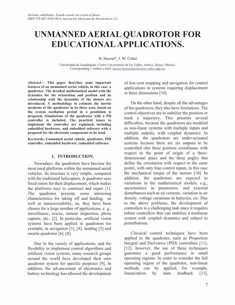
In this section, the mathematical model of the quadrotor is presented, based on the Newton-Euler method. A reference frame is defined at first. There are two frames, a fix frame in the earth, which is used as a reference frame, and a frame in the body of the quadrotor, as it is shown in figure 1 [10].
Figure 1. Reference frame of the quadrotor.
The absolute linear position of the
quadrotor is defined in an inertial frame with the linear position vector ! "# % &'. Moreover, the linear speed is given by ( ! " #( %( &('. The rotation of the quadrotor frame is given by the Euler angles, pitch (rotation in the axis x), roll (rotation in the axis y) and yaw (rotation in the axis z), that define the rotation vector ) !" * + ,', while its time derivative is )( !"*( +( ,( '. Then, the quadrotor is a system described by 12 state variables. Due to some
Sistemas embebidos: Estado actual con visión al futuro
ISBN 978-607-9394-08-0, Asociación Mexicana de Mecatrónica A.C.
9
state variables are related to the reference frame and other are related to the quadrotor frame, it is necessary to define a relation between both frames, of the form:
- ! . /,/+ 0,/+ 10+/,0+0* 1 /*0, /,/* 2 0,0+0* /+0*0,0* 2 /,0+/* 0,0+/* 1 /,0* /+/*3, (1)
where c and s are the sine and cosine functions, respectively. In order to compute any orientation of the quadrotor reference frame, the rotation matrix (1) must be used, i. e., to change between both reference frames. Moreover, the angular speeds of the quadrotor can be obtained from the time derivatives of the angular positions pitch, roll and yaw, as follows:
5 ! .1 0 1089+0 /:0* 089*/:0+0 1089* /:0*/:0+3 ;( (2)
2.1. Forces and momentums.
When the quadrotor is moving, different forces are acting from different physical sources. As a result of the quadrotor rotation there are an aerodynamics force and an aerodynamics momentum. For every motor in the quadrotor, the equations of the force and momentum are given by [11]: <= ! >?=Ω=A (3) B= ! >C=Ω=A (4)
where <= and B= are the aerodynamics force and momentum, of the ith motor, respectively, >?= and >C= are the force and momentum constants of the ith motor, respectively, and Ω= is the angular speed of the ith motor. In general, the four motor are equal, then, the contants >?= and >C= can be considered equal too. So, in the rest of the paper these constants will be written as >? and >C. Furthermore, the vector of momentums of the quadrotor can be defined as:
DE ! F G>?H1ΩAA 2 ΩIAJG>?HΩKA 1 ΩAAJ>CHΩKA 2 ΩAA 2 ΩLA 2 ΩIAJM (5)
where G is the distance between the motor and the origin of the reference in the quadrotor. It is worth mentioning that, in order to avoid the Coriolis effect, the rotors must rotate in the appropriate way, in such a way that they have complementary torques, as it is shown in figure 2. In the reference frame, the acceleration of the rotor is given by the forces of the motors, gravity force and linear frictions. In the initial position, the force acting on the quadrotor in the force of the motors, then, the forces are definied as:
NE ! . 001>?HΩKA 2 ΩAA 2 ΩLA 2 ΩIAJ3
(6) On the other hand, the friction force due
to the air is proportional to the linear speed of the quadrotor, i. e.:
NO ! PQ ( , (7)
where PQ is a matrix with constant elements that contains the dynamics translation coefficients. Moreover, the translation equation can be written as follows:
R S ! . 00RT3 2 UNE 1 NO. (8)
with R as the quadrotor mass and T the gravity acceleration. Moreover, the momentum due to the air friction in the quadrotor can be presented as:
DO ! PV)( , (9)
where PV is a matrix of constant elements that contains the aerodynamics rotation coefficients. Finally, the equation of rotational movement can be expressed as:
Sistemas embebidos: Estado actual con visión al futuro
ISBN 978-607-9394-08-0, Asociación Mexicana de Mecatrónica A.C.
10
W5( 2 5 X YZ 2 Z X . 00[VΩV3 ! DE 1 DO (10)
with W as the inertia matrix, Y as the inertia constants matrix and [V as the inertia constant of the motors.
2.2. Motor dynamics.
In general, the quadrotor requires brushless motors with small dimensions, so that the winding inductance can be neglected and the winding voltage corresponds to the sum of the counter-electromotive force and some resistive loses, i. e., [17]: \ ! 8-] 2 >]^QΩ, (11) where the term >]^QΩ represents the counter-electromotive force, >]^Q is the torque constant of the motor, , -] is the winding resistance and 8 is the winding current.
Moreover, the mechanical dynamics can be written as:
[VΩ( ! _] 1 _ , (12)
where, Ω( is the angular speed of the motor, _] !>]^Q8 and _ ! >CΩA is the torque given by the propeller of the motor. Finally, the winding voltage \ as a function of the motor speed can be presented as: \ ! >]^Q abcdefghid 1 >CΩA (13)
2.3. State-space model.
In order to obtain the state-space model of the quadrotor, the state vector is defined as: # ! "#K #A #L #I #j #k #l #m #n #Ko #KK #KA'p ! q# % & * + , #( %( &( *( +( ,( rp
(14) The input vector s ! "tK tA tL tI'p is presented in a matrix form as:
s ! PuvA, (15)
where vA ! "ΩKA ΩAA ΩLA ΩIA'p and
Pu !wxxy
>? >? >? >?0 1>? 0 >?>? 0 1>? 0>C 1>C >C 1>Cz{{|.
Then, the speed of the motores can be
obtained from (15) as v ! sqrtHPubKsJ, (16)
with sqrtH∙J as the square root of each element in the vector PubKs.
In order to obtain the state space representation the angular accelerations are obtained, that is [10]:
*S ! 1�A#KKΩV 2 �K#KK#KA 2 �KtA (17) +S ! �I#KoΩV 2 �L#Ko#KA 2 �AtL (18) ,S ! �j#Ko#KK 2 �LtI (19)
where �K ! ���b������ , �A ! �����, �L ! ���b������ , �I ! �����,
�j ! ���b������ , �K ! `���, �A ! `��� and �L ! `���.
Now, it is necessary to obtain the linear
accelerations in terms of the state variables. The linear accelerations depends on the rotational and translational state variables, then: #S ! 1 K] H0�9#I0�9#k 2 /:0#I /:0#k0�9#jJtK, (20)
%S ! 1 K] H/: I0�9#k0�9#j 1 /:0 k0�9#jJtK, (21)
&S ! T 1 K] /:0#j/: ktK. (22)
Finally, taking into account (1)-(22), the
state-space nonlinear mathematical model of the quadrotor is presented as follows:
Sistemas embebidos: Estado actual con visión al futuro
ISBN 978-607-9394-08-0, Asociación Mexicana de Mecatrónica A.C.
11
�( ! �H�J 2 �H�, sJ, (23)
where
�H�J !
wxxxxxxxxxxy
#l#m#n#Ko#KK#KA00T1�A#KKΩV 2 �K#KK#KA�I#KoΩV 2 �L#Ko#KA�j#Ko#KK z{{{{{{{{{{|
and
�H�, sJ !
wxxxxxxxxxxxxy
0000001 K] H0�9 I0�9#k 2 /:0#I /:0#k0�9#jJtK1 K] H/:0 I0�9 k0�9#j 1 /:0#k0�9 jJtK1 K] /:0#j/:0#ktK�KtA�AtL�LtI z{{{{{{{{{{{{|
.
2.4. Estimation of inertia constants.
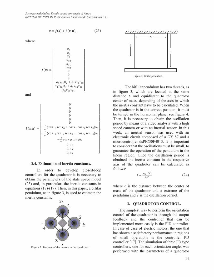
In order to develop closed-loop controllers for the quadrotor it is necessary to obtain the parameters of the state space model (23) and, in particular, the inertia constants in equations (17)-(19). Then, in this paper, a bifilar pendulum, as in figure 3, is used to estimate the inertia constants.
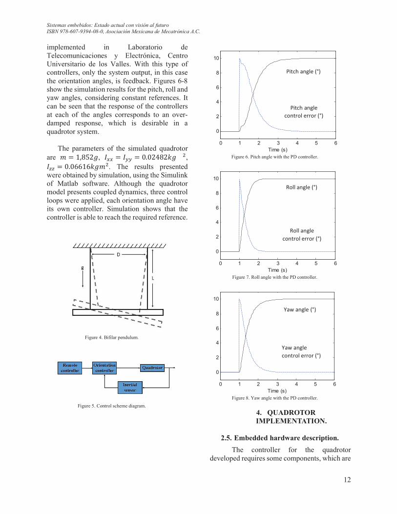
Figure 2. Torques of the motors in the quadrotor.
Figure 3. Bifilar pendulum.
The bifiliar pendulum has two threads, as
in figure 3, which are located at the same distance L and equidistant to the quadrotor center of mass, depending of the axis in which the inertia constant have to be calculated. When the quadrotor is in the correct position, it must be turned in the horizontal plane, see figure 4. Then, it is necessary to obtain the oscillation period by means of a video analysis with a high speed camera or with an inertial sensor. In this work, an inertial sensor was used with an electronic circuit composed of a GY 87 and a microcontroller dsPIC30F4013. It is important to consider that the oscillations must be small, to guarantee the operation of the pendulum in the linear region. Once the oscillation period is obtained the inertia constant in the respective axis of the quadrotor can be calculated as follows:
� ! ]� �p�I�� (24)
where c is the distance between the center of mass of the quadrotor and a extreme of the pendulum and T is the oscillation period.
3. QUADROTOR CONTROL.
The simplest way to perform the orientation control of the quadrotor is through the output feedback and the controller that can be implemented more easily is the PID controller. In case of case of electric motors, the one that has shown a satisfactory performance in regions of small operations is the controller PD controller [17]. The simulation of three PD type controllers, one for each orientation angle, was performed with the parameters of a quadrotor
Sistemas embebidos: Estado actual con visión al futuro
ISBN 978-607-9394-08-0, Asociación Mexicana de Mecatrónica A.C.
12
implemented in Laboratorio de Telecomunicaciones y Electrónica, Centro Universitario de los Valles. With this type of controllers, only the system output, in this case the orientation angles, is feedback. Figures 6-8 show the simulation results for the pitch, roll and yaw angles, considering constant references. It can be seen that the response of the controllers at each of the angles corresponds to an over-damped response, which is desirable in a quadrotor system.
The parameters of the simulated quadrotor
are R ! 1,852T, ��� ! ��� ! 0.02482�T A, ��� ! 0.06616�TRA. The results presented were obtained by simulation, using the Simulink of Matlab software. Although the quadrotor model presents coupled dynamics, three control loops were applied, each orientation angle have its own controller. Simulation shows that the controller is able to reach the required reference.
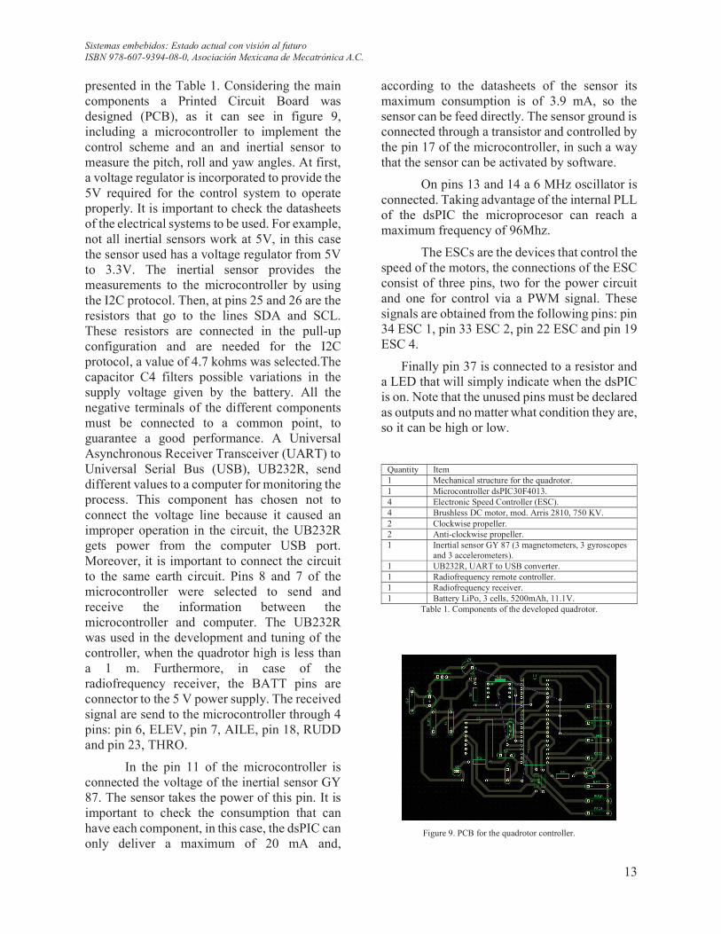
Figure 4. Bifilar pendulum.
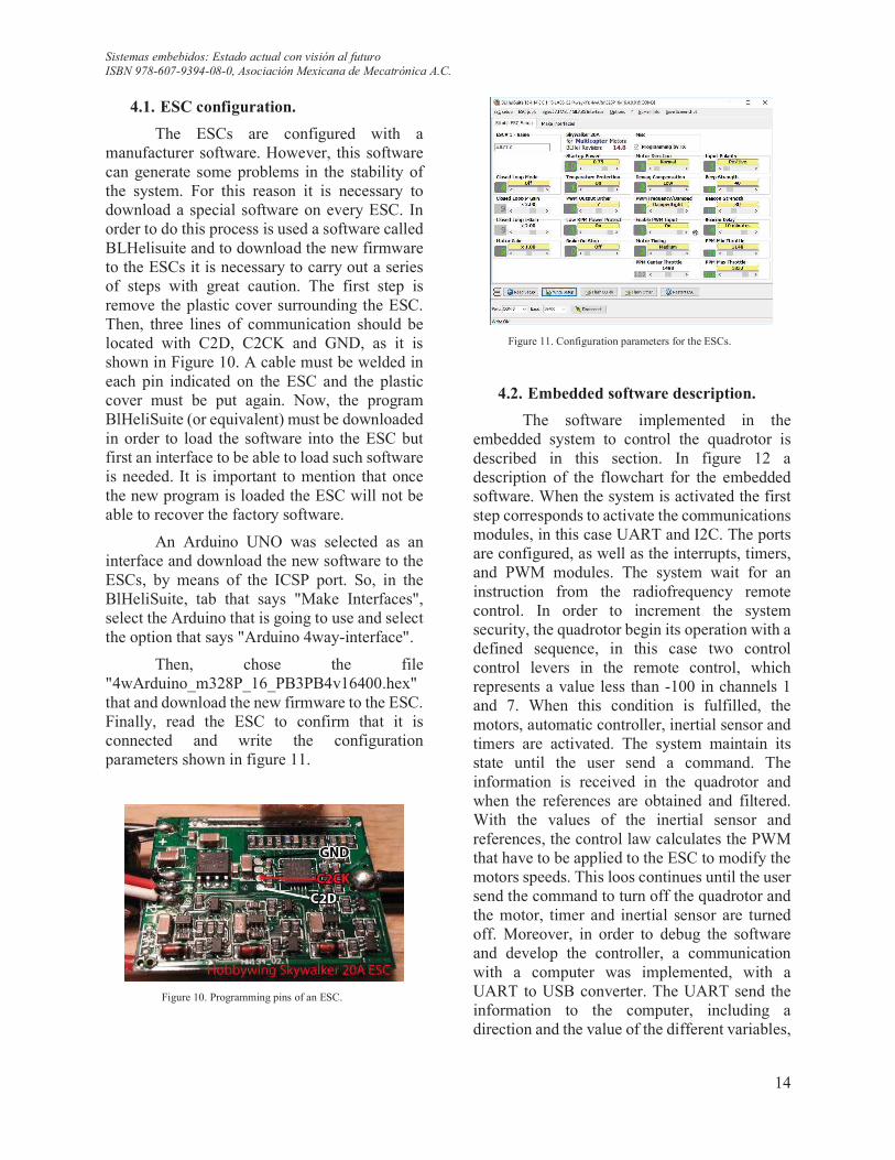
Figure 5. Control scheme diagram.
Figure 6. Pitch angle with the PD controller.
Figure 7. Roll angle with the PD controller.
Figure 8. Yaw angle with the PD controller.
4. QUADROTOR IMPLEMENTATION.
2.5. Embedded hardware description.
The controller for the quadrotor developed requires some components, which are
0 1 2 3 4 5 6
0
2
4
6
8
10
Time (s)
0 1 2 3 4 5 6
0
2
4
6
8
10
Time (s)
0 1 2 3 4 5 6
0
2
4
6
8
10
Time (s)
Pitch angle (°)
Pitch angle
control error (°)
Roll angle (°)
Roll angle
control error (°)
Yaw angle (°)
Yaw angle
control error (°)
Sistemas embebidos: Estado actual con visión al futuro
ISBN 978-607-9394-08-0, Asociación Mexicana de Mecatrónica A.C.
13
presented in the Table 1. Considering the main components a Printed Circuit Board was designed (PCB), as it can see in figure 9, including a microcontroller to implement the control scheme and an and inertial sensor to measure the pitch, roll and yaw angles. At first, a voltage regulator is incorporated to provide the 5V required for the control system to operate properly. It is important to check the datasheets of the electrical systems to be used. For example, not all inertial sensors work at 5V, in this case the sensor used has a voltage regulator from 5V to 3.3V. The inertial sensor provides the measurements to the microcontroller by using the I2C protocol. Then, at pins 25 and 26 are the resistors that go to the lines SDA and SCL. These resistors are connected in the pull-up configuration and are needed for the I2C protocol, a value of 4.7 kohms was selected.The capacitor C4 filters possible variations in the supply voltage given by the battery. All the negative terminals of the different components must be connected to a common point, to guarantee a good performance. A Universal Asynchronous Receiver Transceiver (UART) to Universal Serial Bus (USB), UB232R, send different values to a computer for monitoring the process. This component has chosen not to connect the voltage line because it caused an improper operation in the circuit, the UB232R gets power from the computer USB port. Moreover, it is important to connect the circuit to the same earth circuit. Pins 8 and 7 of the microcontroller were selected to send and receive the information between the microcontroller and computer. The UB232R was used in the development and tuning of the controller, when the quadrotor high is less than a 1 m. Furthermore, in case of the radiofrequency receiver, the BATT pins are connector to the 5 V power supply. The received signal are send to the microcontroller through 4 pins: pin 6, ELEV, pin 7, AILE, pin 18, RUDD and pin 23, THRO.
In the pin 11 of the microcontroller is connected the voltage of the inertial sensor GY 87. The sensor takes the power of this pin. It is important to check the consumption that can have each component, in this case, the dsPIC can only deliver a maximum of 20 mA and,
according to the datasheets of the sensor its maximum consumption is of 3.9 mA, so the sensor can be feed directly. The sensor ground is connected through a transistor and controlled by the pin 17 of the microcontroller, in such a way that the sensor can be activated by software.
On pins 13 and 14 a 6 MHz oscillator is connected. Taking advantage of the internal PLL of the dsPIC the microprocesor can reach a maximum frequency of 96Mhz.
The ESCs are the devices that control the speed of the motors, the connections of the ESC consist of three pins, two for the power circuit and one for control via a PWM signal. These signals are obtained from the following pins: pin 34 ESC 1, pin 33 ESC 2, pin 22 ESC and pin 19 ESC 4.
Finally pin 37 is connected to a resistor and a LED that will simply indicate when the dsPIC is on. Note that the unused pins must be declared as outputs and no matter what condition they are, so it can be high or low.
Quantity Item 1 Mechanical structure for the quadrotor. 1 Microcontroller dsPIC30F4013. 4 Electronic Speed Controller (ESC). 4 Brushless DC motor, mod. Arris 2810, 750 KV. 2 Clockwise propeller. 2 Anti-clockwise propeller. 1 Inertial sensor GY 87 (3 magnetometers, 3 gyroscopes
and 3 accelerometers). 1 UB232R, UART to USB converter. 1 Radiofrequency remote controller. 1 Radiofrequency receiver. 1 Battery LiPo, 3 cells, 5200mAh, 11.1V.
Table 1. Components of the developed quadrotor.
Figure 9. PCB for the quadrotor controller.
Sistemas embebidos: Estado actual con visión al futuro
ISBN 978-607-9394-08-0, Asociación Mexicana de Mecatrónica A.C.
14
4.1. ESC configuration.
The ESCs are configured with a manufacturer software. However, this software can generate some problems in the stability of the system. For this reason it is necessary to download a special software on every ESC. In order to do this process is used a software called BLHelisuite and to download the new firmware to the ESCs it is necessary to carry out a series of steps with great caution. The first step is remove the plastic cover surrounding the ESC. Then, three lines of communication should be located with C2D, C2CK and GND, as it is shown in Figure 10. A cable must be welded in each pin indicated on the ESC and the plastic cover must be put again. Now, the program BlHeliSuite (or equivalent) must be downloaded in order to load the software into the ESC but first an interface to be able to load such software is needed. It is important to mention that once the new program is loaded the ESC will not be able to recover the factory software.
An Arduino UNO was selected as an interface and download the new software to the ESCs, by means of the ICSP port. So, in the BlHeliSuite, tab that says "Make Interfaces", select the Arduino that is going to use and select the option that says "Arduino 4way-interface".
Then, chose the file "4wArduino_m328P_16_PB3PB4v16400.hex" that and download the new firmware to the ESC. Finally, read the ESC to confirm that it is connected and write the configuration parameters shown in figure 11.
Figure 10. Programming pins of an ESC.
Figure 11. Configuration parameters for the ESCs.
4.2. Embedded software description.
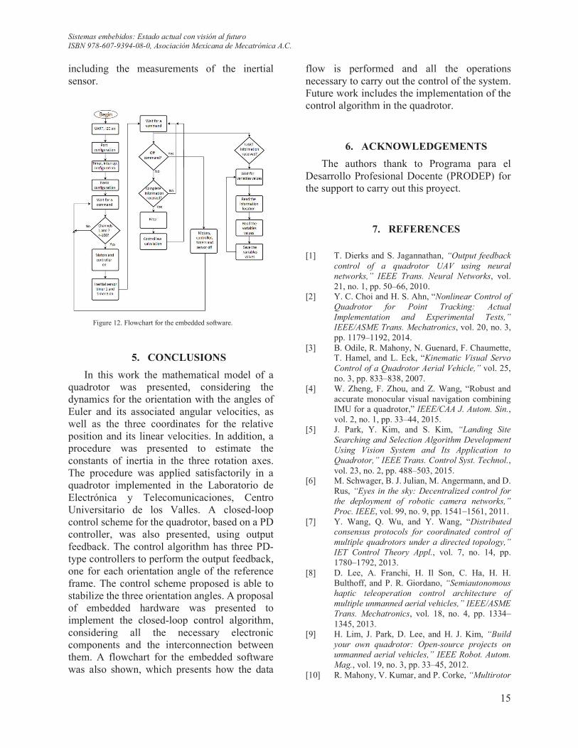
The software implemented in the embedded system to control the quadrotor is described in this section. In figure 12 a description of the flowchart for the embedded software. When the system is activated the first step corresponds to activate the communications modules, in this case UART and I2C. The ports are configured, as well as the interrupts, timers, and PWM modules. The system wait for an instruction from the radiofrequency remote control. In order to increment the system security, the quadrotor begin its operation with a defined sequence, in this case two control control levers in the remote control, which represents a value less than -100 in channels 1 and 7. When this condition is fulfilled, the motors, automatic controller, inertial sensor and timers are activated. The system maintain its state until the user send a command. The information is received in the quadrotor and when the references are obtained and filtered. With the values of the inertial sensor and references, the control law calculates the PWM that have to be applied to the ESC to modify the motors speeds. This loos continues until the user send the command to turn off the quadrotor and the motor, timer and inertial sensor are turned off. Moreover, in order to debug the software and develop the controller, a communication with a computer was implemented, with a UART to USB converter. The UART send the information to the computer, including a direction and the value of the different variables,
Sistemas embebidos: Estado actual con visión al futuro
ISBN 978-607-9394-08-0, Asociación Mexicana de Mecatrónica A.C.
15
including the measurements of the inertial sensor.
Figure 12. Flowchart for the embedded software.
5. CONCLUSIONS
In this work the mathematical model of a quadrotor was presented, considering the dynamics for the orientation with the angles of Euler and its associated angular velocities, as well as the three coordinates for the relative position and its linear velocities. In addition, a procedure was presented to estimate the constants of inertia in the three rotation axes. The procedure was applied satisfactorily in a quadrotor implemented in the Laboratorio de Electrónica y Telecomunicaciones, Centro Universitario de los Valles. A closed-loop control scheme for the quadrotor, based on a PD controller, was also presented, using output feedback. The control algorithm has three PD-type controllers to perform the output feedback, one for each orientation angle of the reference frame. The control scheme proposed is able to stabilize the three orientation angles. A proposal of embedded hardware was presented to implement the closed-loop control algorithm, considering all the necessary electronic components and the interconnection between them. A flowchart for the embedded software was also shown, which presents how the data
flow is performed and all the operations necessary to carry out the control of the system. Future work includes the implementation of the control algorithm in the quadrotor.
6. ACKNOWLEDGEMENTS
The authors thank to Programa para el Desarrollo Profesional Docente (PRODEP) for the support to carry out this proyect.
7. REFERENCES
[1] T. Dierks and S. Jagannathan, “Output feedback
control of a quadrotor UAV using neural
networks,” IEEE Trans. Neural Networks, vol. 21, no. 1, pp. 50–66, 2010.
[2] Y. C. Choi and H. S. Ahn, “Nonlinear Control of
Quadrotor for Point Tracking: Actual
Implementation and Experimental Tests,” IEEE/ASME Trans. Mechatronics, vol. 20, no. 3, pp. 1179–1192, 2014.
[3] B. Odile, R. Mahony, N. Guenard, F. Chaumette, T. Hamel, and L. Eck, “Kinematic Visual Servo
Control of a Quadrotor Aerial Vehicle,” vol. 25, no. 3, pp. 833–838, 2007.
[4] W. Zheng, F. Zhou, and Z. Wang, “Robust and accurate monocular visual navigation combining IMU for a quadrotor,” IEEE/CAA J. Autom. Sin., vol. 2, no. 1, pp. 33–44, 2015.
[5] J. Park, Y. Kim, and S. Kim, “Landing Site
Searching and Selection Algorithm Development
Using Vision System and Its Application to
Quadrotor,” IEEE Trans. Control Syst. Technol., vol. 23, no. 2, pp. 488–503, 2015.
[6] M. Schwager, B. J. Julian, M. Angermann, and D. Rus, “Eyes in the sky: Decentralized control for
the deployment of robotic camera networks,” Proc. IEEE, vol. 99, no. 9, pp. 1541–1561, 2011.
[7] Y. Wang, Q. Wu, and Y. Wang, “Distributed
consensus protocols for coordinated control of
multiple quadrotors under a directed topology,”
IET Control Theory Appl., vol. 7, no. 14, pp. 1780–1792, 2013.
[8] D. Lee, A. Franchi, H. Il Son, C. Ha, H. H. Bulthoff, and P. R. Giordano, “Semiautonomous
haptic teleoperation control architecture of
multiple unmanned aerial vehicles,” IEEE/ASME
Trans. Mechatronics, vol. 18, no. 4, pp. 1334–1345, 2013.
[9] H. Lim, J. Park, D. Lee, and H. J. Kim, “Build
your own quadrotor: Open-source projects on
unmanned aerial vehicles,” IEEE Robot. Autom.
Mag., vol. 19, no. 3, pp. 33–45, 2012. [10] R. Mahony, V. Kumar, and P. Corke, “Multirotor
Sistemas embebidos: Estado actual con visión al futuro
ISBN 978-607-9394-08-0, Asociación Mexicana de Mecatrónica A.C.
16
Aerial Vehicles: Modeling, Estimation, and
Control of Quadrotor,” IEEE Robot. Autom.
Mag., vol. 19, no. 3, pp. 20–32, 2012. [11] B. Erginer and E. Altug, “Modeling and pd
control of a quadrotor pvtol vehicle,” in IEEE
Intelligent Vehicles Symposium, 2007, p. 894–899.
[12] S. Bouabdallah and R. Siegwart, “Full control of
a quadrotor,” in IEEE/RSJ International
Intelligent Robots Systems Conference, 2007, pp. 153–158.
[13] D. Lee, H. J. Kim, and S. Sastry, “Feedback
linearization versus adaptive sliding mode control
for a quadrotor helicopter,” Int. J. Control.
Autom. Syst., vol. 7, no. 3, pp. 419–428, 2009. [14] V. I. Utkin, J. Guldner, and J. Shi, Sliding Mode
Control in Electromechanical Systems. London: Taylor & Francis, 1999.
[15] R. Xu and U. Ozguner, “Sliding mode control of
a quadrotor helicopter,” in IEEE Decision
Control Conference, 2006, pp. 4957–4962. [16] X. Ding and Y. Yu, “Motion planning and
stabilization control of a multipropeller
multifunction aerial robot,” IEEE/ASME
Transanctions on Mechatronics, vol. 18, no. 2, pp. 645–656, 2013.
[17] P. C. Krause, O. Wasynczuk, and S. D. Sudhoff, Analysis of Electric Machinery and Drive
Systems, Second ed. New York, USA, 2002.
Sistemas embebidos: Estado actual con visión al futuro
ISBN 978-607-9394-08-0, Asociación Mexicana de Mecatrónica A.C.
17
CONTROL PROPORCIONAL INTEGRAL CON ANTI WINDUP DE VELOCIDAD EN
MOTORES DE CORRIENTE CONTINUA DE UN ROBOT SEGUIDOR DE LÍNEA
J. A. Zanini Gálvezaa, G. Payano Mirandaa, U. Cortés Ramírezb, A. Castañeda Espinozab
aUniversidad Continental; bUniversidad Tecnológica de Huejotzingo
[email protected], [email protected], [email protected], [email protected]
Abstract— In this paper, we present the design and implementation of an Integral Proportional Control of speed in DC Motors of a robot of the line follower category, with the aim of ensuring that its speed is constant and achieving with this more precise movements. To calculate the transfer function of the motors, we obtained the values in an open loop with LabVIEW, since the system response against the unitary step, the transfer function was estimated with MATLAB, the control was implemented in a development platform Freedom FRDM-KL46Z of NXP(Freescale).
Keywords: Robotics, DC Motor, Control Engineering, Integral Proportional Control, Line Follower Robot.
1. INTRODUCCIÓN
Actualmente la finalidad que tiene la robótica de competencia es mejorar el rendimiento de los robots, de las que existen diversas técnicas para lograr este objetivo. Entre ellas se encuentran los sistemas de control, que se encarga de asegurar que los movimientos del robot sean precisos y fiables. Los sistemas de control facilitan la ejecución de las acciones de acuerdo a la lógica del robot seguidor de línea para la selección entre el seguimiento de las líneas negras o blancas según el escenario que se presente.
En la Universidad Continental, la Escuela Académica Profesional de Ingeniería de Sistemas e Informática posee grupos de investigación y proyectos desarrollados en la línea de investigación de Robótica y Videojuegos, con respecto a los proyectos generados se encuentran los siguientes: 2 robots
soccer (Categoría de competencia Mirosot) y el robot seguidor de línea, mientras que en la Universidad Tecnológica de Huejotzingo, en la carrera de Mecatrónica se han realizado investigaciones con respecto a instrumentación y control aplicado en robots móviles con ruedas, como la plataforma üβot-32b en la que se han instrumentado sus motores de DC obteniendo las variables de posición, velocidad, corriente, torque y temperatura, y a través de sensores inerciales es posible sensar el movimiento del robot y obtener sus variables de posición, velocidad y orientación, este robot actualmente cuenta con un control PI con Anti WindUp para los motores de DC y un control de seguimiento de trayectorias.
El control a implementar es un Proporcional Integral con acción Anti WindUp, para este caso en particular la velocidad del Motor de DC tiene un valor máximo delimitado por el voltaje de alimentación, además de sus características físicas, donde el valor máximo de velocidad estará dado por el valor máximo de la fuente de alimentación, para la salida de control u(t)
cuando toma valores por arriba de los niveles máximos, podemos argumentar que el actuador entrará en saturación o más bien cae en un WindUp, esto causado por la acción integral ante cambios bruscos en la señal de error e(t), la acción Anti WindUp tiene la finalidad de evitar que el actuador permanezca fuera de sus límites de saturación, al resetear la integral y recalcular este término1.
La planta a trabajar es un robot seguidor de línea, y el control estará alojado en una
Sistemas embebidos: Estado actual con visión al futuro
ISBN 978-607-9394-08-0, Asociación Mexicana de Mecatrónica A.C.
18
plataforma Freedom FRDM-KL-46Z, en la que como primera instancia realizará la lectura de los encóders para obtener la posición y velocidad de los motores de DC, una vez obtenidas estas variables se adquirirá la respuesta de los motores en lazo abierto y se capturaran en un archivo Excel a través de LabVIEW, estos datos se exportarán a MATLAB para estimar la función de transferencia del motor de DC empleado la herramienta System Identification, el diseño del controlador Proporcional Integral se realizará con la aplicación PID Tuning.
1.1. Robot seguidor de línea
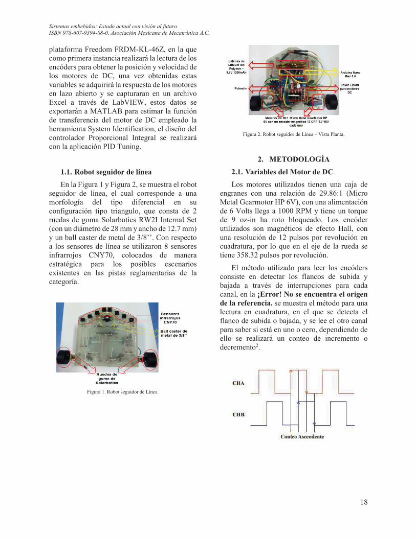
En la Figura 1 y Figura 2, se muestra el robot seguidor de línea, el cual corresponde a una morfología del tipo diferencial en su configuración tipo triangulo, que consta de 2 ruedas de goma Solarbotics RW2I Internal Set (con un diámetro de 28 mm y ancho de 12.7 mm) y un ball caster de metal de 3/8’’. Con respecto a los sensores de línea se utilizaron 8 sensores infrarrojos CNY70, colocados de manera estratégica para los posibles escenarios existentes en las pistas reglamentarias de la categoría.
Figura 1. Robot seguidor de Línea.
Figura 2. Robot seguidor de Línea – Vista Planta.
2. METODOLOGÍA
2.1. Variables del Motor de DC
Los motores utilizados tienen una caja de engranes con una relación de 29.86:1 (Micro Metal Gearmotor HP 6V), con una alimentación de 6 Volts llega a 1000 RPM y tiene un torque de 9 oz-in ha roto bloqueado. Los encóder utilizados son magnéticos de efecto Hall, con una resolución de 12 pulsos por revolución en cuadratura, por lo que en el eje de la rueda se tiene 358.32 pulsos por revolución.
El método utilizado para leer los encóders consiste en detectar los flancos de subida y bajada a través de interrupciones para cada canal, en la ¡Error! No se encuentra el origen de la referencia. se muestra el método para una lectura en cuadratura, en el que se detecta el flanco de subida o bajada, y se lee el otro canal para saber si está en uno o cero, dependiendo de ello se realizará un conteo de incremento o decremento2.
Sistemas embebidos: Estado actual con visión al futuro
ISBN 978-607-9394-08-0, Asociación Mexicana de Mecatrónica A.C.
19
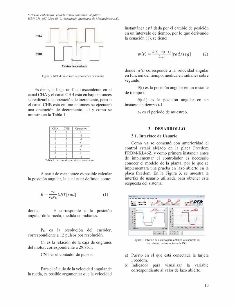
Figura 3. Método de conteo de encóder en cuadratura
Es decir, si llega un flaco ascendente en el canal CHA y el canal CHB está en bajo entonces se realizará una operación de incremento, pero si el canal CHB está en uno entonces se ejecutará una operación de decremento, tal y como se muestra en la Tabla 1.
CHA CHB Operación ↑ 0 +1 ↑ 1 -1 0 ↑ -1 1 ↑ +1 ↓ 0 -1 ↓ 1 +1 0 ↓ +1 1 ↓ -1
Tabla 1. Lectura de encoder en cuadratura
A partir de este conteo es posible calcular la posición angular, la cual estar definida como:
+ ! A����� � _"¡�¢' (1)
donde: θ corresponde a la posición angular de la rueda, medida en radianes.
PE es la resolución del encóder, correspondiente a 12 pulsos por resolución.
CE es la relación de la caja de engranes del motor, correspondiente a 29.86:1.
CNT es el contador de pulsos.
Para el cálculo de la velocidad angular de la rueda, es posible argumentar que la velocidad
instantánea está dada por el cambio de posición en un intervalo de tiempo, por lo que derivando la ecuación (1), se tiene:
£H¤J ! ¥HQJb¥HQbKJ∆Qd "¡�¢ 0�T⁄ ' (2)
donde: w(t) corresponde a la velocidad angular en función del tiempo, medida en radianes sobre segundo.
θ(t) es la posición angular en un instante de tiempo t.
θ(t-1) es la posición angular en un instante de tiempo t-1.
tm es el periodo de muestreo.
3. DESARROLLO
3.1. Interface de Usuario
Como ya se comentó con anterioridad el control estará alojado en la placa Freedom FRDM-KL46Z, y como primera instancia antes de implementar el controlador es necesario conocer el modelo de la planta, por lo que se implementará una prueba en lazo abierto en la placa freedom. En la Figura 3, se muestra la interfaz de usuario utilizada para obtener esta respuesta del sistema.
Figura 3. Interfaz de usuario para obtener la respuesta en
lazo abierto de los motores de DC.
a) Puerto en el que está conectada la tarjeta Freedom.
b) Indicador para visualizar la variable correspondiente al valor de lazo abierto.
Sistemas embebidos: Estado actual con visión al futuro
ISBN 978-607-9394-08-0, Asociación Mexicana de Mecatrónica A.C.
20
c) Indicador para visualizar la variable correspondiente al valor deseado.
d) Botón para detener el programa. e) Trazo de datos en tiempo real. f) Trazo de datos de una prueba realizada.
Esta interface de usuario se desarrolló en el entorno de LabVIEW, en la que a través de un puerto de comunicación COM se capturan los datos que son recibidos de la tarjeta Freedom y posteriormente se exportaron a Excel, estos datos corresponden al valor de entrada (wd) y el valor de salida (w), cada captura se realizó con un periodo de muestreo de 1ms. La velocidad deseada fue del 50% del máximo posible por el motor (siendo esta 57 rad/s); además el tiempo de prueba realizado fue de 1.5 segundos con una referencia positiva y de 1.5 segundos una referencia negativa.
La interfaz de usuario tiene la finalidad de capturar la respuesta del sistema, en la que inicialmente se obtendrá la respuesta en lazo abierto y una vez que se implemente el control en la placa Freedom se estará obteniendo la respuesta de este, para sucesivamente ir exportando todos los datos de cada una de las pruebas a Excel con la finalidad de comparar las respuesta de todas las pruebas realizadas.
3.2. Estimación de la función de transferencia
Para obtener la respuesta de los motores en lazo abierto se aplicó una velocidad de referencia u(t) y se observó la respuesta natural del sistema y(t), como se ilustra en la Figura 4.
Figura 4. Respuesta en lazo abierto.
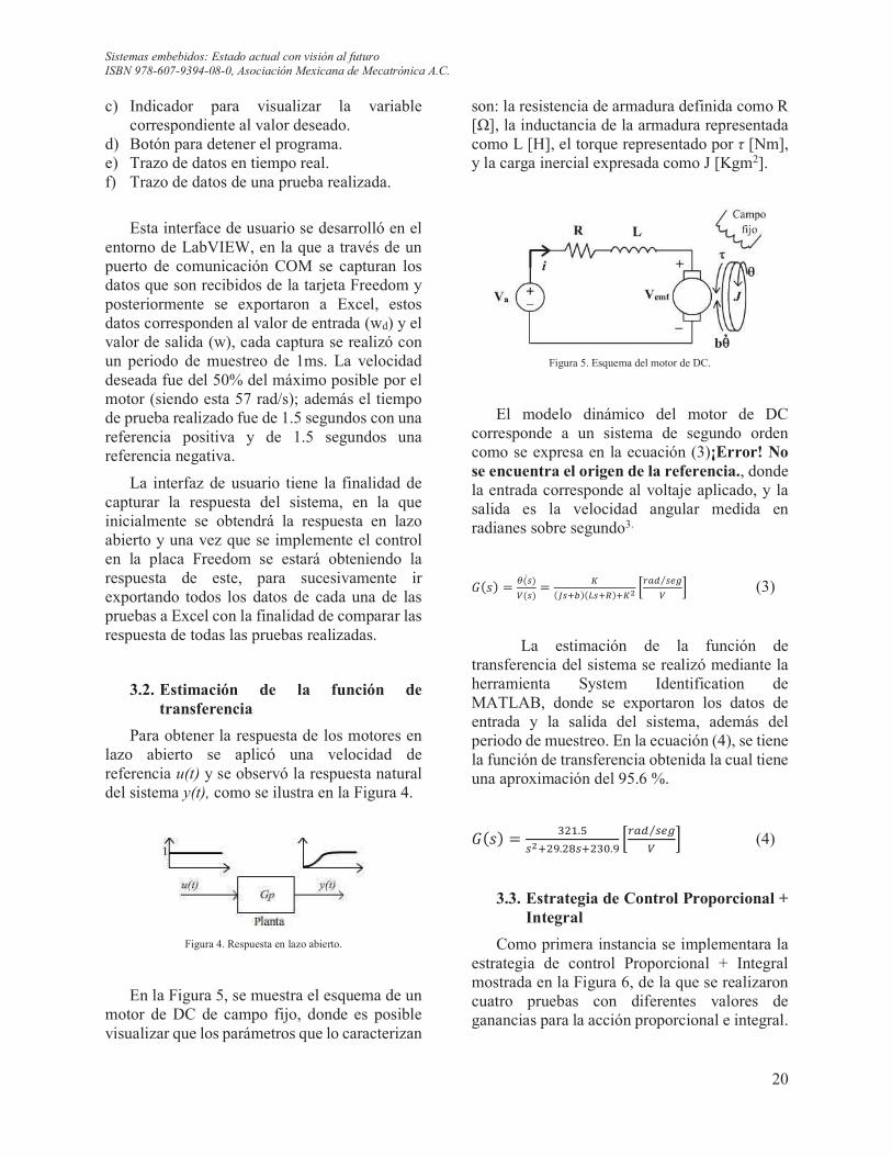
En la Figura 5, se muestra el esquema de un motor de DC de campo fijo, donde es posible visualizar que los parámetros que lo caracterizan
son: la resistencia de armadura definida como R [Ω], la inductancia de la armadura representada como L [H], el torque representado por τ [Nm], y la carga inercial expresada como J [Kgm2].
Figura 5. Esquema del motor de DC.
El modelo dinámico del motor de DC corresponde a un sistema de segundo orden como se expresa en la ecuación (3)¡Error! No se encuentra el origen de la referencia., donde la entrada corresponde al voltaje aplicado, y la salida es la velocidad angular medida en radianes sobre segundo3.
¨H0J ! ¥H©J(ªH©J ! cH�©«¬JH©«iJ«c� ®VO¯ ©°�⁄ª ± (3)
La estimación de la función de transferencia del sistema se realizó mediante la herramienta System Identification de MATLAB, donde se exportaron los datos de entrada y la salida del sistema, además del periodo de muestreo. En la ecuación (4), se tiene la función de transferencia obtenida la cual tiene una aproximación del 95.6 %.
¨H0J ! LAK.j©�«An.Am©«ALo.n ®VO¯ ©°�⁄ª ± (4)
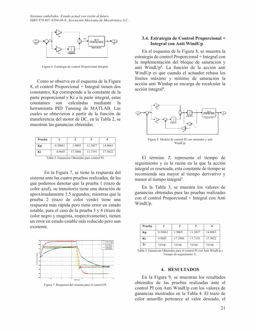
3.3. Estrategia de Control Proporcional + Integral
Como primera instancia se implementara la estrategia de control Proporcional + Integral mostrada en la Figura 6, de la que se realizaron cuatro pruebas con diferentes valores de ganancias para la acción proporcional e integral.
Sistemas embebidos: Estado actual con visión al futuro
ISBN 978-607-9394-08-0, Asociación Mexicana de Mecatrónica A.C.
21
Figura 6. Estrategia de control Proporcional Integral.
Como se observa en el esquema de la Figura 8, el control Proporcional + Integral tienen dos constantes, Kp corresponde a la constante de la parte proporcional y Ki a la parte integral, estas constantes son calculadas mediante la herramienta PID Tunning de MATLAB. Las cuales se obtuvieron a partir de la función de transferencia del motor de DC, en la Tabla 2, se muestran las ganancias obtenidas.
Prueba 1 2 3 4
Kp 0.30861 1.9005 11.3827 14.8063
Ki 4.9605 17.3886 11.7191 17.5022
Tabla 2. Ganancias Obtenidas para control PI.
En la Figura 7, se tiene la respuesta del sistema ante las cuatro pruebas realizadas, de las que podemos denotar que la prueba 1 (trazo de color azul), su transitorio tiene una duración de aproximadamente 1.5 segundos, mientras que la prueba 2 (trazo de color verde) tiene una respuesta más rápida pero tiene error en estado estable, para el caso de la prueba 3 y 4 (trazo de color negro y magenta, respectivamente), tienen un error en estado estable más reducido pero aun existente.
Figura 7. Respuesta del sistema para el control PI.
3.4. Estrategia de Control Proporcional + Integral con Anti WindUp
En el esquema de la Figura 8, se muestra la estrategia de control Proporcional + Integral con la implementación del bloque de saturación y anti WindUp4. La función de la acción anti WindUp es que cuando el actuador rebasa los límites máximo y mínimo de saturación la acción anti Windup se encarga de recalcular la acción integral4.
Figura 8. Modelo de control PI con saturador y anti
WindUp.
El término Tt representa el tiempo de seguimiento y es la razón en la que la acción integral es reseteada, esta constante de tiempo se recomienda sea mayor al tiempo derivativo y menor al tiempo integral1.
En la Tabla 3, se muestra los valores de ganancias obtenidas para las pruebas realizadas con el control Proporcional + Integral con Anti WindUp.
Prueba 1 2 3 4
Kp 0.30861 1.9005 11.3827 14.8063
Ki 4.9605 17.3886 11.7191 17.5022
Tt 1µseg 1µseg 1µseg 1µseg
Tabla 3. Ganancias Obtenidas para el control PI con Anti WindUp y Tiempo de seguimiento Tt.
4. RESULTADOS
En la Figura 9, se muestran los resultados obtenidos de las pruebas realizadas ante el control PI con Anti WindUp con los valores de ganancias mostrados en la Tabla 4. El trazo de color amarillo pertenece al valor deseado, el
Sistemas embebidos: Estado actual con visión al futuro
ISBN 978-607-9394-08-0, Asociación Mexicana de Mecatrónica A.C.
22
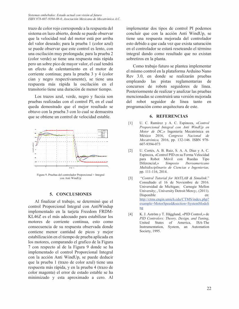
trazo de color rojo corresponde a la respuesta del sistema en lazo abierto, donde se puede observar que la velocidad real del motor está por arriba del valor deseado; para la prueba 1 (color azul) se puede observar que este control es lento, con una oscilación muy prolongada; para la prueba 2 (color verde) se tiene una respuesta más rápida pero un sobre pico de mayor valor, el cual tendrá un efecto de calentamiento en el motor de corriente continua; para la prueba 3 y 4 (color cian y negro respectivamente), se tiene una respuesta más rápida la oscilación en el transitorio tiene una duración de menor tiempo.
Los trazos azul, verde, negro y fucsia son pruebas realizadas con el control PI, en el cual queda demostrado que el mejor resultado se obtuvo con la prueba 3 con lo cual se demuestra que se obtiene un control de velocidad estable.
Figura 9. Pruebas del controlador Proporcional + Integral
con Anti WindUp
5. CONCLUSIONES
Al finalizar el trabajo, se determinó que el control Proporcional Integral con AntiWindup implementado en la tarjeta Freedom FRDM-KL46Z es el más adecuado para estabilizar los motores de corriente continua, esto como consecuencia de su respuesta observada donde contiene menor cantidad de picos y mejor estabilización en el tiempo de prueba aplicada en los motores, comparando el grafico de la Figura 7 con respecto al de la Figura 9 donde se ha implementado el control Proporcional Integral con la acción Anti WindUp, se puede deducir que la prueba 1 (trazo de color azul) tiene una respuesta más rápida, y en la prueba 4 (trazo de color magenta) el error de estado estable se ha minimizado y esta aproximado a cero. Al
implementar dos tipos de control PI podemos concluir que con la acción Anti WindUp, se tiene una respuesta mejorada del controlador esto debido a que cada vez que exista saturación en el controlador se estará reseteando el término integral dando como resultado que no existan sobretiros en la planta.
Como trabajo futuro se plantea implementar el mismo control en la plataforma Arduino Nano Rev 3.0, en donde se realizarán pruebas empleando las pistas reglamentarias de concursos de robots seguidores de línea. Posteriormente de realizar y analizar las pruebas mencionadas se construirá una versión mejorada del robot seguidor de línea tanto en programación como arquitectura de este.
6. REFERENCIAS
[1] U. C. Ramírez y A. C. Espinoza, «Control
Proporcional Integral con Anti WindUp en
Motor de DC,» Ingeniería Mecatrónica en México 2016, Congreso Nacional de
Mecatrónica, 2016, pp. 132-146. ISBN 978-607-9394-073
[2] U. Cortés, A. B. Ruiz, S. A. A. Diaz y A. C. Espinoza, «Control PID en su Forma Velocidad para Robot Móvil con Ruedas Tipo Diferencial,» Simposio Iberoamericano
Multidisciplinario de Ciencias e Ingenierias,
pp. 111-116, 2014.
[3] “Control Tutorial for MATLAB & Simulink.” Consultado el 16 de Noviembre de 2016. Universidad de Michigan; Carnegie Mellon University; , University Detroit Mercy;. (2011). Disponible en: http://ctms.engin.umich.edu/CTMS/index.php?example=MotorSpeed§ion=SystemModeling
[4] K. J. Aström y T. Hägglund, «PID Control,» de PID Controlers: Theory, Design, and Tuning, United States of America, ISA-The Instrumentation, System, an Automation Society, 1995.
Sistemas embebidos: Estado actual con visión al futuro
ISBN 978-607-9394-08-0, Asociación Mexicana de Mecatrónica A.C.
23
DESIGN OF A FUZZY C-MEANS ALGORITHM FOR AIR POLLUTION
PREDICTION BASED ON AN EMBEDDED PLATFORM
Juan M. De la Cruz-Aguirre1, Marco A. Aceves-Fernández1, Juan Manuel Ramos-Arreguín2, José Emilio Vargas-Soto2
1 Facultad de Informática, Universidad Autónoma de Querétaro, Querétaro, México
2 Facultad de Ingeniería, Universidad Autónoma de Querétaro, Querétaro, México
[email protected], [email protected]
Abstract— The airborne particles PM10 and PM25 are some of the most dangerous pollutants for the human health due to the minimum aerodynamic diameter that they have. The design of a Fuzzy-C means algorithm for Air Pollution prediction based on VHDL represents a feasible and reliable solution, which is validated comparing its performance with a powerful existent simulation tool.
I. INTRODUCTION
The action of breathing implies a permanent contact of the respiratory system with the environment. Although this relation is fundamental for life, it makes us also vulnerable to the pollutant materials contained in breathable air. The lungs are the entry open, invisible most of the times, for a large number of substances capable of generating breathing, cardiac, and other organs diseases. Clean air is a shared concern among scientists and institutions [1], and not only the big cities are the target, but also medium scale cities as demonstrated in a researching conducted from 2012 in Xiamen China, which corroborates a progressive and significant increasing of PM particles exposure [2].
Studies as the one mentioned in [3] have been fundamental to determine that air quality is vital for health and welfare; this quality depends on the presence in the atmosphere of pollutants in quantities superior to the allowed levels for the human being. Urban planning is also of paramount importance for air quality also, because mobility and industrial process aspects determine, in conjunction with meteorological conditions, the emission, distribution and the diffusion of atmospheric pollutants. The following are the predominant pollutants: Sulphur dioxide (SO2), nitrogen dioxide (NO2), carbon monoxide (CO), volatile organic compounds (VOC), the total suspended particles (TSP) and plumb [4].
Two of the most dangerous pollutants from the suspended particles are the PM10 and PM2.5. They have a featured aerodynamic diameter below 10 µm and 2.5 µm respectively, and they are considered riskier than other ones with bigger diameters, mainly the 2.5 particles; because of the less diameter the most capable to penetrate
deeper the respiratory tract conducting to the region of air interchange, transgressing more through other organs. Additionally, they contain a greater quantity of toxins due to the compounds forming them.
The effects these particles have in the human health varies from minor symptoms like nose and throat irritations to the most severe consequences in the respiratory system, cardiovascular diseases, and even premature death, increasing the probability in the elderly as described in [3]. The key aspects contributing this pollution are the heavy industry activity, the over-pollution, and city traffic. Besides these factors, other secondary sources as the contaminant gases through the gas-to-particle conversion, and the re-suspension of particles due to human or earth movements, also serve as a source of PM2.5 which contains several metal elements. Other pollution generators are the infiltration of particles due to the combustion like the automotive smog and the waste incineration. The permissible levels are 15.0 µg/m3 (micrograms per cubic meter) although in some cases these can reach 35 µg/m3 and 50 µg/m3 in the more contaminated cities. According to the Official Mexican Law (NOM for its Spanish acronym), NOM-025-SSA1-2014 [5], the acceptable levels of PM10 particles is 75 µg/m3 for a 24 hours average, and 40 µg/m3 annual average limit. For the PM2.5 particles, this law specifies 45 µg/m3 for a 24 hours average and 12 µg/m3 annual average limit.
Therefore, air pollution controls to prevent worst measurements in the long and the short terms are needed. Several research works have been performed, modeling the space-time to prevent hourly concentrations in USA cities in [6]. The current pollutant particles prediction scheme proposes a clustering based algorithm according to the Fuzzy C-Means (FCM) technique used in [7].
In traditional clustering or other modeling systems such as [8], [9] or [10], one entity belongs to one single cluster. In the FCM technique, it is allowed for one item to belong to several clusters based on their location on the histogram and with different degrees of membership. This versatility
Sistemas embebidos: Estado actual con visión al futuro
ISBN 978-607-9394-08-0, Asociación Mexicana de Mecatrónica A.C.
24
provides major certainty to the pollutant particles prediction.
II. METHODOLOGY
A. The Fuzzy-Clustering Algorithm
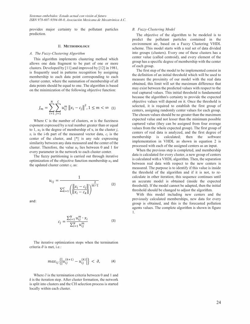
This algorithm implements clustering method which allows one data fragment to be part of one or more clusters. Developed by [11] and improved by [12] in 1981, is frequently used in patterns recognition by assigning membership to each data point corresponding to each cluster center, where the summation of membership of all data points should be equal to one. The algorithm is based on the minimization of the following objective function:
[] ! ² ² t=³] ´#= 1 /³´A, 1 µ R ¶ ∞�³¸K
¹=¸K
Where C is the number of clusters, m is the fuzziness exponent expressed by a real number greater than or equal to 1, uij is the degree of membership of xi in the cluster j, xi is the i-th part of the measured vector data, cj is the center of the cluster, and ||*|| is any rule expressing similarity between any data measured and the center of the cluster. Therefore, the value uij lies between 0 and 1 for every parameter in the network to each cluster center.
The fuzzy partitioning is carried out through iterative optimization of the objective function membership uij and the updated cluster center cj as:
t=³ ! 1∑ »´#= 1 /³´‖#= 1 /½‖¾ A]bK�½¸K
and:
/³ ! ∑ t=³] ∙ #=¹=¸K∑ t=³]¹=¸K The iterative optimization stops when the termination
criteria ¿ is met, i.e.:
R�#=³ ÀÁt=³H½«KJ 1 t=³H½JÁ ¶ ¿, Where ∂ is the termination criteria between 0 and 1 and
k is the iteration step. After cluster formation, the network is split into clusters and the CH selection process is started locally within each cluster.
B. Fuzzy-Clustering Model
The objective of the algorithm to be modeled is to predict the pollutant particles contained in the environment air, based on a Fuzzy Clustering VHDL scheme. This model starts with a real set of data divided into groups (clusters). Every one of these clusters has a center value (called centroid), and every element of the group has a specific degree of membership with the center of each group.
The first step of the model to be implemented consist in the definition of an initial threshold which will be used to measure the proximity of our model with the real data obtained, this limit will set the maximum difference that may exist between the predicted values with respect to the real captured values. This initial threshold is fundamental because the algorithm's certainty to provide the expected objective values will depend on it. Once the threshold is selected, it is required to establish the first group of centers, assigning randomly center values for each group. The chosen values should be no greater than the maximum expected value and not lesser than the minimum possible captured value (they can be assigned from four average values from the whole expected group). The first group of centers of real data is analyzed, and the first degree of membership is calculated; then the software implementation in VHDL as shown in equation 2 is processed with each of the assigned centers as an input.
When the previous step is completed, and membership data is calculated for every cluster, a new group of centers is calculated with a VHDL algorithm. Then, the separation between real data with respect to the new centers is measured. The purpose is to identify if this value is inside the threshold of the algorithm and if it is not, to re-calculate in other iteration; this sequence continues until an accurate model is obtained (inside the expected threshold). If the model cannot be adapted, then the initial threshold should be changed to adjust the algorithm.
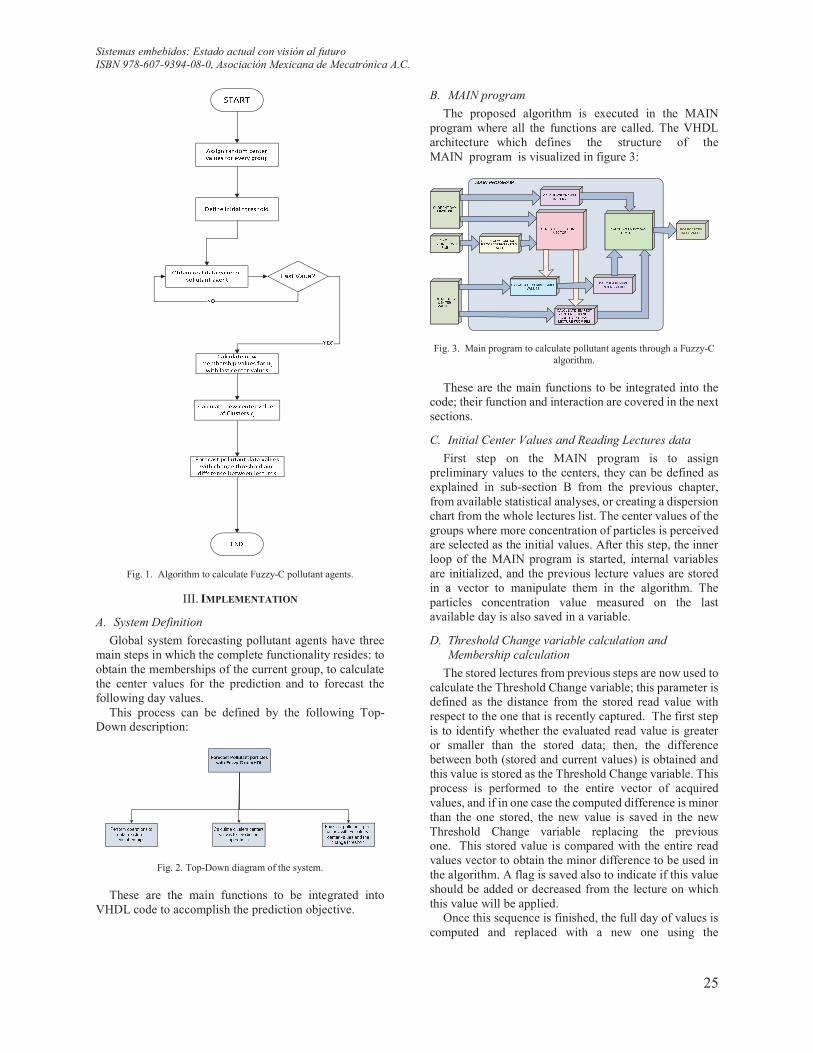
With this model including new centers and the previously calculated memberships, new data for every group is obtained, and this is the forecasted pollution agents values. The complete algorithm is shown in figure 1.
(2)
(3)
(1)
(4)
Sistemas embebidos: Estado actual con visión al futuro
ISBN 978-607-9394-08-0, Asociación Mexicana de Mecatrónica A.C.
25
Fig. 1. Algorithm to calculate Fuzzy-C pollutant agents.
III. IMPLEMENTATION
A. System Definition
Global system forecasting pollutant agents have three main steps in which the complete functionality resides: to obtain the memberships of the current group, to calculate the center values for the prediction and to forecast the following day values.
This process can be defined by the following Top-Down description:
Fig. 2. Top-Down diagram of the system. These are the main functions to be integrated into
VHDL code to accomplish the prediction objective.
B. MAIN program
The proposed algorithm is executed in the MAIN program where all the functions are called. The VHDL architecture which defines the structure of the MAIN program is visualized in figure 3:
Fig. 3. Main program to calculate pollutant agents through a Fuzzy-C algorithm.
These are the main functions to be integrated into the
code; their function and interaction are covered in the next sections.
C. Initial Center Values and Reading Lectures data
First step on the MAIN program is to assign preliminary values to the centers, they can be defined as explained in sub-section B from the previous chapter, from available statistical analyses, or creating a dispersion chart from the whole lectures list. The center values of the groups where more concentration of particles is perceived are selected as the initial values. After this step, the inner loop of the MAIN program is started, internal variables are initialized, and the previous lecture values are stored in a vector to manipulate them in the algorithm. The particles concentration value measured on the last available day is also saved in a variable.
D. Threshold Change variable calculation and
Membership calculation
The stored lectures from previous steps are now used to calculate the Threshold Change variable; this parameter is defined as the distance from the stored read value with respect to the one that is recently captured. The first step is to identify whether the evaluated read value is greater or smaller than the stored data; then, the difference between both (stored and current values) is obtained and this value is stored as the Threshold Change variable. This process is performed to the entire vector of acquired values, and if in one case the computed difference is minor than the one stored, the new value is saved in the new Threshold Change variable replacing the previous one. This stored value is compared with the entire read values vector to obtain the minor difference to be used in the algorithm. A flag is saved also to indicate if this value should be added or decreased from the lecture on which this value will be applied.
Once this sequence is finished, the full day of values is computed and replaced with a new one using the

Sistemas embebidos: Estado actual con visión al futuro
ISBN 978-607-9394-08-0, Asociación Mexicana de Mecatrónica A.C.
26
Threshold Change variable, the following diagram is the Top-Down figure describing this step.
Fig. 4. Top-Down diagram for Threshold Change variable calculation. This new group of lectures will be the input to calculate
a new group of Memberships. This computation is performed with the center value for every particle using the formulas from section II.
The representation below describes how this is implemented. For every read value, there would be a degree of membership corresponding to each evaluated center.
Fig. 5. Top-Down Diagram for Membership Algorithm
E. New center values calculation and Near center
definition
The definition of the near center to each following-day lecture is the next step. The next-day data acquisition is obtained by taken the previous next-day value but now adding or subtracting the Threshold change value. During this process, every center is compared against the calculated next-day lecture. When all the centers are processed, the nearest center is flagged, and also another parameter is stored to indicate if this distance should be added or subtracted.
At this point, all the operations needed with the current center values have been completed and a new set should be computed with the last obtained membership values; this new centers will settle the basis for the forecasting of the pollutant elements of the next-day. The first step is to compute for each acquired data of the new group, its corresponding membership degree, by adding-up the membership of each value powered to the Fuzzifier value, and to multiply this by the evaluated acquired data as described in previous sections, figure 6 shows the Top-Down description for this sequence.
Fig. 6. Top-Down Diagram for New Centers calculations
F. Next-day lecture forecast
The membership values obtained in the first steps of the algorithm and the new center values calculated in previous sections will allow us to predict the next-day value. The Threshold Change variable flag is used, to indicate if this should be added or subtracted, and it is also used in conjunction with the flag to indicate if the nearest center distance should also be added or subtracted. These two values are applied to the stored next-day lecture for the corresponding center cluster to which this value belongs. After those operations, the forecasted next-day value is obtained, and the image below shows how this process should be performed.

Sistemas embebidos: Estado actual con visión al futuro
ISBN 978-607-9394-08-0, Asociación Mexicana de Mecatrónica A.C.
27
Fig. 7. Top-Down Diagram to predict the following-day lecture During the next section, another platform (Matlab) will
be used to validate the results obtained with the VHDL implementation.
IV. SIMULATION AND VALIDATION
A. VHDL System simulation
A pollutant particles forecast system should be capable of interacting with cities where this is a serious pollution concern. Therefore, for the simulation and verification stages, real data is used. Previously stored data is evaluated and divided into files of 8760 samples each, which represent one year of stored information of Nitrogen Dioxide NO2 particles, and 10 nanometers of diameter PM10 particles. In order to achieve similar conditions for weather and humidity, the data is divided into four parts corresponding to every season of the year, in this way there are equal conditions for every data file being used for forecasting.
When the application is started, every iteration presents the analyzed data in vector groups, and the algorithm produces the forecasting of the most probable pollutant data that will be measured on the Next-day. The following figure shows the input vectors and the processed data when the simulation is started. In the top part of the variables list, the membership vectors which are used for the cycle execution are visualized. Also, the center values utilized for the simulation, the initial input lectures, the resultant membership values and the operation system variables for every cycle are displayed.
Fig. 8. Input vectors and processing of Fuzzy-Clustering algorithm on VHDL
A vector containing the Next-day forecasting results is
obtained. As the iterations are executed the application continues showing the acquired values for the Next-day readings. Figure 9 shows this step:
Fig. 9. Output vector including following-day prediction
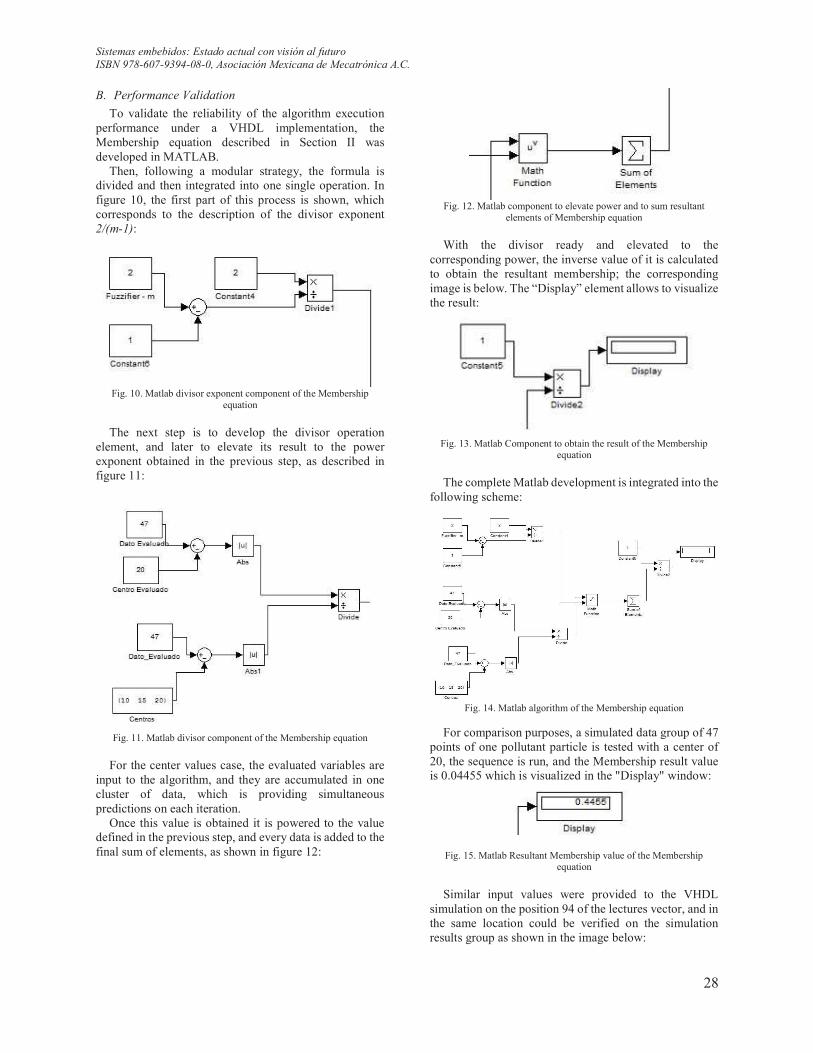
Sistemas embebidos: Estado actual con visión al futuro
ISBN 978-607-9394-08-0, Asociación Mexicana de Mecatrónica A.C.
28
B. Performance Validation
To validate the reliability of the algorithm execution performance under a VHDL implementation, the Membership equation described in Section II was developed in MATLAB.
Then, following a modular strategy, the formula is divided and then integrated into one single operation. In figure 10, the first part of this process is shown, which corresponds to the description of the divisor exponent 2/(m-1):
Fig. 10. Matlab divisor exponent component of the Membership
equation The next step is to develop the divisor operation
element, and later to elevate its result to the power exponent obtained in the previous step, as described in figure 11:
Fig. 11. Matlab divisor component of the Membership equation
For the center values case, the evaluated variables are
input to the algorithm, and they are accumulated in one cluster of data, which is providing simultaneous predictions on each iteration.
Once this value is obtained it is powered to the value defined in the previous step, and every data is added to the final sum of elements, as shown in figure 12:
Fig. 12. Matlab component to elevate power and to sum resultant
elements of Membership equation
With the divisor ready and elevated to the corresponding power, the inverse value of it is calculated to obtain the resultant membership; the corresponding image is below. The “Display” element allows to visualize the result:
Fig. 13. Matlab Component to obtain the result of the Membership
equation
The complete Matlab development is integrated into the following scheme:
Fig. 14. Matlab algorithm of the Membership equation
For comparison purposes, a simulated data group of 47
points of one pollutant particle is tested with a center of 20, the sequence is run, and the Membership result value is 0.04455 which is visualized in the "Display" window:
Fig. 15. Matlab Resultant Membership value of the Membership
equation Similar input values were provided to the VHDL
simulation on the position 94 of the lectures vector, and in the same location could be verified on the simulation results group as shown in the image below:
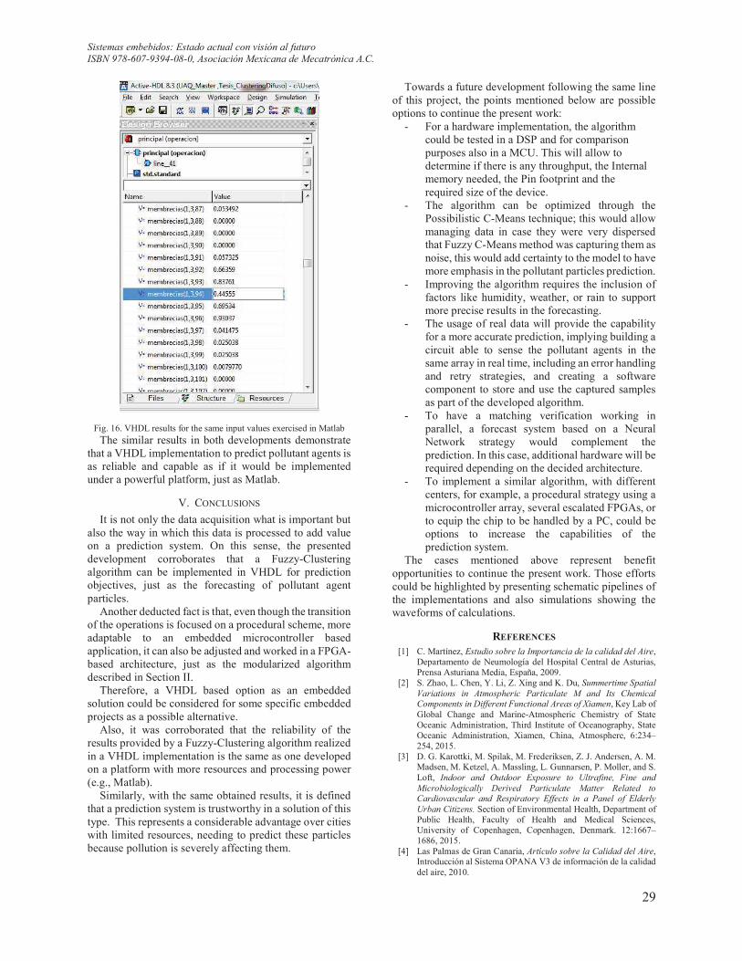
Sistemas embebidos: Estado actual con visión al futuro
ISBN 978-607-9394-08-0, Asociación Mexicana de Mecatrónica A.C.
29
Fig. 16. VHDL results for the same input values exercised in Matlab The similar results in both developments demonstrate
that a VHDL implementation to predict pollutant agents is as reliable and capable as if it would be implemented under a powerful platform, just as Matlab.
V. CONCLUSIONS
It is not only the data acquisition what is important but also the way in which this data is processed to add value on a prediction system. On this sense, the presented development corroborates that a Fuzzy-Clustering algorithm can be implemented in VHDL for prediction objectives, just as the forecasting of pollutant agent particles.
Another deducted fact is that, even though the transition of the operations is focused on a procedural scheme, more adaptable to an embedded microcontroller based application, it can also be adjusted and worked in a FPGA-based architecture, just as the modularized algorithm described in Section II.
Therefore, a VHDL based option as an embedded solution could be considered for some specific embedded projects as a possible alternative.
Also, it was corroborated that the reliability of the results provided by a Fuzzy-Clustering algorithm realized in a VHDL implementation is the same as one developed on a platform with more resources and processing power (e.g., Matlab).
Similarly, with the same obtained results, it is defined that a prediction system is trustworthy in a solution of this type. This represents a considerable advantage over cities with limited resources, needing to predict these particles because pollution is severely affecting them.
Towards a future development following the same line of this project, the points mentioned below are possible options to continue the present work:
- For a hardware implementation, the algorithm could be tested in a DSP and for comparison purposes also in a MCU. This will allow to determine if there is any throughput, the Internal memory needed, the Pin footprint and the required size of the device.
- The algorithm can be optimized through the Possibilistic C-Means technique; this would allow managing data in case they were very dispersed that Fuzzy C-Means method was capturing them as noise, this would add certainty to the model to have more emphasis in the pollutant particles prediction.
- Improving the algorithm requires the inclusion of factors like humidity, weather, or rain to support more precise results in the forecasting.
- The usage of real data will provide the capability for a more accurate prediction, implying building a circuit able to sense the pollutant agents in the same array in real time, including an error handling and retry strategies, and creating a software component to store and use the captured samples as part of the developed algorithm.
- To have a matching verification working in parallel, a forecast system based on a Neural Network strategy would complement the prediction. In this case, additional hardware will be required depending on the decided architecture.
- To implement a similar algorithm, with different centers, for example, a procedural strategy using a microcontroller array, several escalated FPGAs, or to equip the chip to be handled by a PC, could be options to increase the capabilities of the prediction system.
The cases mentioned above represent benefit opportunities to continue the present work. Those efforts could be highlighted by presenting schematic pipelines of the implementations and also simulations showing the waveforms of calculations.
REFERENCES [1] C. Martínez, Estudio sobre la Importancia de la calidad del Aire,
Departamento de Neumología del Hospital Central de Asturias, Prensa Asturiana Media, España, 2009.
[2] S. Zhao, L. Chen, Y. Li, Z. Xing and K. Du, Summertime Spatial
Variations in Atmospheric Particulate M and Its Chemical Components in Different Functional Areas of Xiamen, Key Lab of Global Change and Marine-Atmospheric Chemistry of State Oceanic Administration, Third Institute of Oceanography, State Oceanic Administration, Xiamen, China, Atmosphere, 6:234–254, 2015.
[3] D. G. Karottki, M. Spilak, M. Frederiksen, Z. J. Andersen, A. M. Madsen, M. Ketzel, A. Massling, L. Gunnarsen, P. Moller, and S. Loft, Indoor and Outdoor Exposure to Ultrafine, Fine and
Microbiologically Derived Particulate Matter Related to Cardiovascular and Respiratory Effects in a Panel of Elderly
Urban Citizens. Section of Environmental Health, Department of Public Health, Faculty of Health and Medical Sciences, University of Copenhagen, Copenhagen, Denmark. 12:1667–1686, 2015.
[4] Las Palmas de Gran Canaria, Artículo sobre la Calidad del Aire, Introducción al Sistema OPANA V3 de información de la calidad del aire, 2010.
Sistemas embebidos: Estado actual con visión al futuro
ISBN 978-607-9394-08-0, Asociación Mexicana de Mecatrónica A.C.
30
[5] Official Mexican Law for Environmental Healthy, Permissible values for suspended particles PM10 and PM2.5 concentrations in the environment and their evaluation criteria, Healthy Secretary, Federal Government of Mexico, NOM-025-SSA1, 2014.
[6] S. Batterman, R. Ganguly and P. Harbin, High Resolution Spatial
and Temporal Mapping of Traffic-Related Air Pollutants, Environmental Health Sciences, School of Public Health, University of Michigan, Ann Arbor, MI, U.S., 12:3646–3666, 2015.
[7] D. M. Saqib Bhatti, N. Saeed, H. Nam, Fuzzy C-Means Clustering
and Energy Efficient Cluster Head Selection for Cooperative
Sensor Network, Department of Electronics and Communication Engineering, Hanyang University, Ansan 15588, Korea, Sensors, 16, 1459; doi:10.3390/s16091459, 2016.
[8] A. Balamashc, W. Pedrycza, R. Al-Hmouzc and A. Morfeqc, An expansion of fuzzy information granules through successive
refinements of their information content and their use to system
modeling, Department of Electrical & Computer Engineering, University of Alberta, Edmonton, Canada, 2014.
[9] M. Caselli, L. Trizio, G. De Gennaro and P. Lelpo, A Simple
Feedforward Neural Network for the PM10 Forecasting: Comparison with a Radial Basis Function Network and a
Multivariate Linear Regression Model, Water Air Soil Pollution, 201:365–377, 2009.
[10] A.B. Chelani and M. Z. Hasan, Forecasting nitrogen dioxide
concentration in ambient air using artificial Neural-networks, Air Pollution Control Division, National Environmental Engineering Research Institute (NEERI), Nagpur, India, International Journal of Environmental Studies, 58(4):487–499, 2001.
[11] J.C. Dunn, A Fuzzy Relative of the ISODATA Process and Its Use in Detecting Compact Well-Separated Clusters, 32–57, 1973.
[12] J.C. Bezdek, Pattern Recognition with Fuzzy Objective Function
Algorithms, Kluwer Academic Publishers, Norwell, MA, U.S., 1981.
Sistemas embebidos: Estado actual con visión al futuro
ISBN 978-607-9394-08-0, Asociación Mexicana de Mecatrónica A.C.
31
INTERNET DE LAS COSAS Y REDES DE SENSORES INALÁMBRICOS: REVIEW Paul Roseroa,b, Santiago Núñeza, Stalin Realpea, Vanessa Alveara,b, Luis Beltránb, Christian Rosadob.
a Universidad Técnica del Norte; b Instituto Tecnológico Superior 17 de Julio [email protected]
Resumen— La evolución de Internet ha tenido un alto impacto para la población mundial, aunque en sus inicios solo se consideró como una red de computadores ha pasado a convertirse en la base del desarrollo de la mayoría de aspectos de la vida diaria de todas las personas. La relación entre dispositivos conectados y el número de usuarios que se ha establecido en los últimos años indica que existen más sistemas electrónicos conectados a Internet que habitantes a nivel mundial. El Internet de las Cosas (IoT) se origina por la necesidad de estar conectados entre todos, esto incluye a personas y cosas, de tal manera que cada individuo pueda gestionar de forma remota a cualquier objeto que tenga una conexión a Internet. Esto ha requerido emplear diversas tecnologías, la que mayor éxito ha tenido son las redes de sensores inalámbricos, debido a que permiten recoger diferentes tipos de datos para luego poder ser monitorizados y gestionados. Varias organizaciones a nivel mundial se han encargado de trabajar en la arquitectura y los protocolos que se deben tomar en cuenta para desarrollar aplicaciones de IoT con el fin de que exista compatibilidad entre dispositivos. Una revisión del estado del arte de IoT y WSN permite tener una visión más amplia del alcance, arquitectura, aplicaciones y limitaciones de estas tecnologías, especialmente enfocados al manejo de seguridad de la información y Big Data. Keywords: Aplicaciones de IoT, Internet de las cosas,
Redes de sensores inalámbricos.
1. INTRODUCCIÓN
La sociedad actual está haciendo que la tecnología evolucione con mayor frecuencia, la necesidad del siglo XXI es intercomunicar todos los dispositivos electrónicos con las personas, esto implica que tanto hardware como software sean mucho más sofisticados. [1] establece que las redes de comunicaciones se encuentran por todas partes, cableadas e inalámbricas, facilitando la forma de acceder al medio de comunicación. Las personas lo llaman como “Internet del Futuro”. Internet de las Cosas (IoT) es la comunicación de personas y dispositivos
mediante un enlace a la red Internet, Cisco define el término Internet de Todo (IoE) como una versión actualizada de IoT y se refiere a personas, datos y cosas administrados por un componente identificado como un proceso [2]. El alcance va más allá de la comunicación máquina a máquina (M2M, por sus siglas en inglés Machine to Machine) por ser robusto en protocolos, aplicaciones y dominios de red [3]. Es un entorno total que interactúa con nuetras actividades cotidianas para brindarnos confort en relación a nuestras necesidades.
Una red de sensores inalámbricos (WSN) ha sido reconocida como la tecnología más emergente e interesante para el desarrollo de IoT. Le ha permitido aumentar su popularidad en la investigación industrial y académica. Los nuevos productos WSN están impulsando la próxima ola de crecimiento exponencial, actuando como nodos sensores en el desarrollo de una gama de aplicaciones [4].
En el presente trabajo se presentan los
protocolos existentes, desempeño y resultados en múltiples aplicaciones. Contemplando las dificultades y retos que debe cumplir el IoT, como el crecimiento del número de sensores y objetos, obligando a tener mayores consideraciones en seguridad de la información, el rápido aprendizaje de los datos y la selección correcta de la información para delimitar la gran cantidad de datos que se van a presentar por esta tecnología (Big Data).
A continuación, se presenta como se encuentra dividido este trabajo, la sección 2 abarca la Evolución del Internet de las cosas al Internet de Todo, en la sección 3 se muestra la Arquitectura de IoT, más adelante la sección 4
Sistemas embebidos: Estado actual con visión al futuro
ISBN 978-607-9394-08-0, Asociación Mexicana de Mecatrónica A.C.
32
habla de las Redes de Sensores Inalámbricos e IoT, la sección 5 detalla los protocolos usados de Internet de las Cosas en una WSN, las aplicaciones de IoT en un WSN se muestran en la sección 6, finalmente la sección 7 recopila las conclusiones y recomendaciones de este trabajo.
2. EVOLUCIÓN DE INTERNET DE LAS COSAS A INTERNET DE TODO
Los entornos IoT han evolucionado a un concepto más amplio conocido como Internet del todo (IoE). [5] menciona que este tipo de aplicaciones han ido ganando impulso en el mercado durante los últimos años. No es sólo el hecho de que el número de dispositivos inteligentes y sensores van en aumento año tras año, sino también las actividades industriales de la población.
IoT es la comunicación de personas y dispositivos mediante un enlace a la red Internet, según Cisco 50 mil millones de cosas estarán conectadas a Internet en 2020, si bien las proyecciones pueden variar, es inevitable que los objetos se conecten al mundo del IoT [6], abriendo nuevas oportunidades y desafíos que se enfrentarán durante los años siguientes. Enormes cantidades de datos se generan y consumen, por lo que el IoT tendrá que proporcionar nuevas capacidades relacionadas con el análisis de grandes volúmenes de datos, escalabilidad y rendimiento.
Según [2] IoE es la evolución de seres inteligentes (Gente), Procesos, Datos y Cosas, para convertir la información en nuevas experiencias y oportunidades económicas para instituciones, empresas e individuos. Un factor determinante que se quiere lograr mediante el IoE es la entrega de información correcta a la persona o máquina de manera eficiente y eficaz. A continuación, se indica cada uno de los elementos que se relacionan en el Internet de Todo:
A. Gente: La mayoría de las personas se conectan a Internet a través de múltiples dispositivos sociales. El sector de la educación necesita entender cómo las
personas se conectan a Internet para aumentar su aprendizaje.
B. Proceso: Es la forma de trabajar datos y cosas para ofrecer un valor, las conexiones se vuelven relevantes y se añade valor debido a que la información correcta se entrega a la persona adecuada en el momento preciso.
C. Datos: El Internet evoluciona y debe proveer un modo de información más útil, los objetos deben enviar información del más alto nivel para su posterior evaluación y toma de decisiones más rápida.
D. Cosas: Las cosas son objetos físicos que se pueden conectar tanto a Internet como a la gente a través de sensores, proporcionando información para ayudar a las personas y máquinas a tomar decisiones relevantes y valiosas.
3. ARQUITECTURA DE INTERNET DE LAS COSAS
El IoT debe tener la capacidad de interconectar millones o billones de diversos objetos a través de Internet, por lo tanto, la arquitectura debe poseer capas flexibles. Existen muchas propuestas de arquitectura de IoT, como la que define [7], arquitectura IoThNet orientada directamente en el cuidado de la salud, que facilita transmisión y recepción de datos médicos. De igual manera se han estructurado modelos como el que presenta [8] planteado para hacer frente a los problemas de seguridad, sin embargo, aún no se converge en una sola arquitectura.
A la par se desarrollan algunos proyectos que tratan de diseñar una arquitectura común basada en el análisis de las necesidades de los investigadores y la industria. De todas las propuestas de arquitecturas IoT, se resaltan modelos desde los más básicos que tiene 3 capas, hasta otros que poseen 5 capas, teniendo en cuenta que no es el modelo de referencia TCP/IP [9], [10] y [11] concuerdan en la siguiente arquitectura que posee 5 capas, a
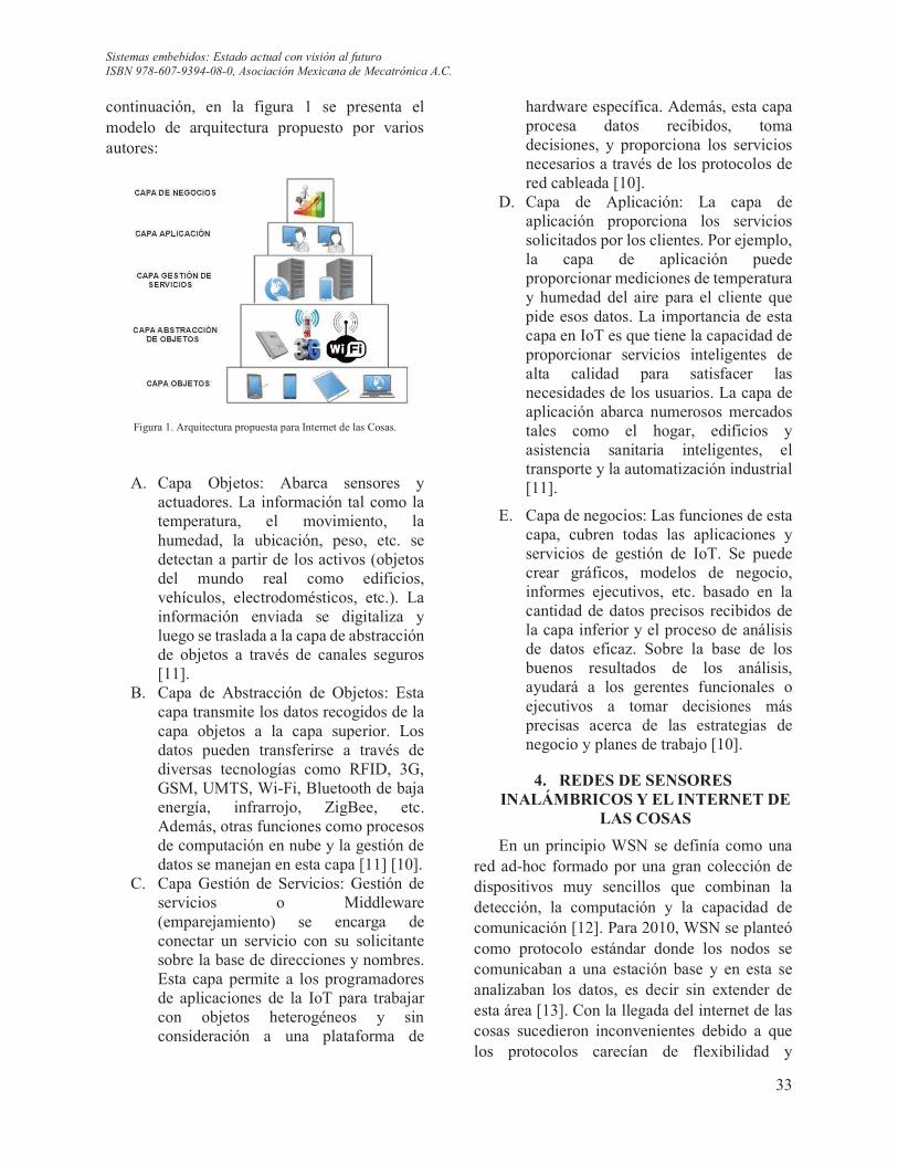
Sistemas embebidos: Estado actual con visión al futuro
ISBN 978-607-9394-08-0, Asociación Mexicana de Mecatrónica A.C.
33
continuación, en la figura 1 se presenta el modelo de arquitectura propuesto por varios autores:
Figura 1. Arquitectura propuesta para Internet de las Cosas.
A. Capa Objetos: Abarca sensores y actuadores. La información tal como la temperatura, el movimiento, la humedad, la ubicación, peso, etc. se detectan a partir de los activos (objetos del mundo real como edificios, vehículos, electrodomésticos, etc.). La información enviada se digitaliza y luego se traslada a la capa de abstracción de objetos a través de canales seguros [11].
B. Capa de Abstracción de Objetos: Esta capa transmite los datos recogidos de la capa objetos a la capa superior. Los datos pueden transferirse a través de diversas tecnologías como RFID, 3G, GSM, UMTS, Wi-Fi, Bluetooth de baja energía, infrarrojo, ZigBee, etc. Además, otras funciones como procesos de computación en nube y la gestión de datos se manejan en esta capa [11] [10].
C. Capa Gestión de Servicios: Gestión de servicios o Middleware (emparejamiento) se encarga de conectar un servicio con su solicitante sobre la base de direcciones y nombres. Esta capa permite a los programadores de aplicaciones de la IoT para trabajar con objetos heterogéneos y sin consideración a una plataforma de
hardware específica. Además, esta capa procesa datos recibidos, toma decisiones, y proporciona los servicios necesarios a través de los protocolos de red cableada [10].
D. Capa de Aplicación: La capa de aplicación proporciona los servicios solicitados por los clientes. Por ejemplo, la capa de aplicación puede proporcionar mediciones de temperatura y humedad del aire para el cliente que pide esos datos. La importancia de esta capa en IoT es que tiene la capacidad de proporcionar servicios inteligentes de alta calidad para satisfacer las necesidades de los usuarios. La capa de aplicación abarca numerosos mercados tales como el hogar, edificios y asistencia sanitaria inteligentes, el transporte y la automatización industrial [11].
E. Capa de negocios: Las funciones de esta capa, cubren todas las aplicaciones y servicios de gestión de IoT. Se puede crear gráficos, modelos de negocio, informes ejecutivos, etc. basado en la cantidad de datos precisos recibidos de la capa inferior y el proceso de análisis de datos eficaz. Sobre la base de los buenos resultados de los análisis, ayudará a los gerentes funcionales o ejecutivos a tomar decisiones más precisas acerca de las estrategias de negocio y planes de trabajo [10].
4. REDES DE SENSORES INALÁMBRICOS Y EL INTERNET DE
LAS COSAS
En un principio WSN se definía como una red ad-hoc formado por una gran colección de dispositivos muy sencillos que combinan la detección, la computación y la capacidad de comunicación [12]. Para 2010, WSN se planteó como protocolo estándar donde los nodos se comunicaban a una estación base y en esta se analizaban los datos, es decir sin extender de esta área [13]. Con la llegada del internet de las cosas sucedieron inconvenientes debido a que los protocolos carecían de flexibilidad y
Sistemas embebidos: Estado actual con visión al futuro
ISBN 978-607-9394-08-0, Asociación Mexicana de Mecatrónica A.C.
34
compatibilidad con las aplicaciones ya que requieren modificaciones, una solución muy comercial es el estándar 6loWPAN propuesto como un método viable para llevar IPV6 por medio de WSN.
A diferencia de otras redes, las redes de sensores inalámbricos tienen la característica particular de la recolección de datos detectados (temperatura, presión, movimiento, detección de incendio, voltaje / corriente, etc.) y reenviarlo a la puerta de salida (Gateway) a través de un protocolo de comunicación de una sola vía. Los nodos de sensores en WSN también pueden ser considerados como una colección de bajo costo y consumo de energía con medio inalámbrico multifuncional [14], permitiendo detectar eventos de datos de sensores [15].
5. PROTOCOLOS DE IOT USADOS EN UNA WSN
A. 6 LOW PAN: Es un estándar que ha introducido la noción de redes de sensores inalámbricas basadas en la transmisión de paquetes IPV6 sobre redes IEEE 802.15.4, la aparición de estas redes genera la necesidad de implementar mecanismos de seguridad [16]. La pila de protocolos 6loWPAN incluye la capa estándar MAC IEEE 802.15.4 y capa física IEEE 802.15.4, la capa IP adopta el protocolo IPV6 de IETF, por lo tanto, permite la interconexión entre redes [17]. El enrutamiento RPL, también conocido como el protocolo de capa de red es un protocolo de enrutamiento por vector de distancia para redes de baja energía, usando IPv6. Los dispositivos de red que ejecutan el protocolo RPL se conectan sin ciclos presentes. Propuesto por IETF para el enrutamiento IPv6, RPL está diseñado para redes con tasas de pérdida de paquetes altos, y de baja energía. El objetivo de RPL es apuntar a redes que "comprenden hasta miles de nodos", donde la mayoría de los nodos tienen recursos muy limitados, la red está dirigida por un nodo central. Se incluyen
tráficos multipunto a punto, punto a multipunto y punto a punto [18].
B. MQQT: Protocolo diseñado específicamente para comunicación máquina-a-máquina y las aplicaciones móviles. Está optimizado para las comunicaciones a través de redes, donde el ancho de banda es un bien escaso o cuando la conexión de red podría ser intermitente [20] [21].
6. APLICACIONES DEL INTERNET DE LAS COSAS CON WSN
El internet de las cosas ha evolucionado al punto en que podemos sensar la actividad de todo objeto. Las aplicaciones tienen por objetivo optimizar procesos y garantizar mayores recursos.
En el campo de la investigación se puede encontrar que IoT está brindando soluciones en una alta gama de aplicaciones como: ciudades inteligentes, congestión del tráfico, gestión de residuos, salud, seguridad estructural, servicios de emergencia, logística, ventas al por menor, control industrial, sistemas electrónicos de vehículos, gestión del medio ambiente, gestión del hogar y control de servicios públicos [3] [22].
A. IoT en la Educación: Puede ayudar en actividades educativas ligadas a las matemáticas, la ciencia y la educación física, los estudiantes pueden utilizar sensores para monitorizar su actividad diaria mediante la recopilación de datos sobre la distancia que camina o corre, su ritmo cardíaco y otras funciones metabólicas. Las clases se vuelven más interesantes y los estudiantes utilizan los datos para motivar a los demás a adoptar estilos de vida más saludables [2].
B. Smart surfaces: [23] establece las superficies inteligentes, se trata de una tecnología basada en una cantidad de elementos que proporcionan una función cuando trabajan juntos para comunicar o transmitir información. Este sistema usa etiquetas RFID pasivas las cuales están incrustadas debajo de las cerámicas, un
Sistemas embebidos: Estado actual con visión al futuro
ISBN 978-607-9394-08-0, Asociación Mexicana de Mecatrónica A.C.
35
zapato equipado con un lector, y un transmisor receptor capaz de interrogar al piso y transmitir la información al internet, el objetivo es crear un sistema de localización en interiores de edificios
C. Smart cities: Establece la combinación de tecnologías de la información y las comunicaciones (TIC), para el desarrollo de un crecimiento económico y sostenible para una alta calidad de vida de los ciudadanos. [24] indica que las ciudades inteligentes son una realidad futura para los municipios de todo el mundo. Las autoridades serán líderes visionarios esenciales que impulsen el progreso de la ciudad inteligente para invertir en proyectos escalables.
D. Smart grid: Permite crear servicios inteligentes y constituye una de las aplicaciones más importantes del IoT, ya que permite supervisar la transmisión de energía, para la prevención y mitigación de desastres naturales, es indispensable debido a que sólo existen aplicaciones de tipo manual y dependientes de una persona [25].
E. Industria: El control del proceso de producción, monitoreo ambiental, el seguimiento de la cadena de suministro de fabricación, el seguimiento del ciclo de vida de un producto, la seguridad en la fabricación, ahorro de energía y control de la contaminación [24].
F. Agricultura inteligente: La utilización de los recursos agrícolas, la gestión cuantitativa en el proceso de producción agrícola, monitoreo de la producción y el manejo del cultivo, la gestión de la calidad, la seguridad y la trazabilidad de los productos agrícolas [26].
G. Logística inteligente: Control de inventario, gestión de la distribución, la trazabilidad y otros sistemas de logística modernos, la plataforma de servicios logísticos públicos que cubren diferentes zonas y dominios, con el comercio electrónico y logística inteligentes [25].
H. Transporte inteligente: La percepción del estado del tráfico y sus notificaciones, guía de tráfico y control
inteligente, la posición del vehículo y la programación, el monitoreo remoto del vehículo y el servicio, el vehículo y la coordinación de carreteras [25].
I. Seguridad inteligente: Monitoreo de la seguridad social, la vigilancia del transporte de productos químicos peligrosos y de carga, control de la seguridad alimentaria, alerta temprana y respuesta de emergencia para las infraestructuras tales como puentes, edificios importantes, el tránsito ferroviario, suministro público de agua, el drenaje y la red de tuberías municipales [27].
J. Medicina inteligente: Control inteligente de la medicina, gestión de los hospitales, la recolección y el análisis de los parámetros de fisiología y medicina para humanos, y servicio médico a distancia para la familia y la comunidad [28].
7. CONCLUSIONES Y TRABAJOS FUTUROS
El Internet de las cosas es una tecnología que ha estado en un proceso de evolución, en la actualidad ya es usado para muchas aplicaciones, sin embargo, aún existen parámetros no definidos con claridad como su arquitectura. La migración al protocolo IPv6 permite la conexión de todo dispositivo electrónico a plataformas IoT mediante el uso de redes de sensores con miras a generar mayores aplicaciones para el beneficio de las personas.
Debido a la gran cantidad de dispositivos que se conectarán a Internet, los retos como la seguridad de la información, el análisis de datos, el consumo de baterías etc. Deben ser tomados en cuenta para el diseño y desarrollo de WSN. El hardware para realizar aplicaciones de IoT debe poseer cualidades para trabajar con protocolos y puertas de enlace a Internet, de esta manera se asegurará el manejo de datos de una forma transparente hacia el usuario.
Como trabajos futuros se plantea comparar protocolos dentro de redes de sensores para

Sistemas embebidos: Estado actual con visión al futuro
ISBN 978-607-9394-08-0, Asociación Mexicana de Mecatrónica A.C.
36
conocer su rendimiento en la transferencia datos de diferentes sensores análogos y digitales con el fin de plantear una trama de datos generalizada aplicada a los diferentes estándares de comunicación inalámbrica, posteriormente aplicar algoritmos de machine learning embebido.
8. REFERENCIAS
[1] L. Coetzee y J. Eksteen, «The Internet of Things – Promise for the Future? An Introduction» de IST-Africa Conference Proceedings, 2011, Gaborone, 2011.
[2] M. Selinger, A. Sepulveda y B. Jim, «Education and the Internet of Everything, How Ubiquitous Connectedness Can Help Transform Pedagogy,» Cisco Consulting Services and Cisco EMEAR Education Team, p. 14, 2013.
[3] M. H. Miraz, A. Maaruf y P. S. Excell, «A Review on Internet of Things (loT), Internet of Everything (IoE) and Internet of Nano Things (IoNT),» Internet Technologies and Applications (ITA), 2015, pp. 219 - 224, 8-11 Septiembre 2015.
[4] F. E. Murphy , E. Popovici, P. Whelan y M. Magno, «Development of an heterogeneous wireless sensor network for instrumentation and analysis of beehives,» de 2015 IEEE International Instrumentation and Measurement Technology Conference (I2MTC) Proceedings, Pisa, 2015.
[5] F. J. Nieto de Santos y S. García, «Exploiting Local Clouds in the Internet of Everything Environment,» de Euromicro International Conference on Parallel, Distributed, and Network-Based Processing, Turku, 2015.
[6] N. Khalil, M. Riduan Abid y D. Benhaddou, «Wireless Sensors Networks for Internet of Things,» de Intelligent Sensors, Sensor Networks and Information Processing (ISSNIP), 2014 IEEE Ninth International Conference, Singapore, 2014.
[7] R. Islam , D. Kwak, H. Kabir y M. Hossain, «The Internet of Things for Health Care: A Comprehensive Survey,» de The internet of things approaches to smart healthcare solutions., 2015.
[8] H. Suo , J. Wan, C. Zou y J. Liu, «Security in the Internet of Things: A Review,» de Computer Science and Electronics Engineering (ICCSEE), 2012 International Conference on, Hangzhou, 2012.
[9] J. Kaur y K. Kaur , «Availing Internet of Things in Industrial Decision Making -A Survey,» International Conference on Electrical, Electronics, and Optimization Techniques (ICEEOT) , pp. 1, 2, 2016.
[10] S. Kraijak y P. Tuwanut, «A SURVEY ON IOT ARCHITECTURES, PROTOCOLS, APPLICATIONS, SECURITY, PRIVACY, REAL-WORLD IMPLEMENTATION AND FUTURE TRENDS,» Proceedings of ICCT, p. 27, 2015.
[11] A. Al-Fuqaha, M. Guizani, M. Mohammadi, M. Aledhari y M. Ayyash, «Internet of Things: A Survey on Enabling Technologies, Protocols, and Applications,» IEEE COMMUNICATION SURVEYS & TUTORIALS, vol. 17, nº 4, pp. 2, 7, 8, 9, 10, 2015.
[12] T. Bokareva, N. Bulusu y S. Jha, «A Performance Comparison of Data Dissemination Protocols for Wireless Sensor Networks,» de Global Telecommunications Conference Workshops, 2004. GlobeCom Workshops 2004. IEEE, 2004.
[13] A. Castellani , N. Bui, P. Casari, M. Rossi y Z. Shelby, «Architecture and protocols for the Internet of Things: A case study,» de Pervasive Computing and Communications Workshops (PERCOM Workshops), 2010 8th IEEE International Conference on, Mannheim, 2010.
[14] R. Singh Bisht y S. Budhani , «Performance analysis of hierarchical and nonhierarchical routing techniques in wireless sensor networks,» de Soft Computing Techniques for Engineering and Technology (ICSCTET), 2014 International Conference on, Bhimtal,
2014.
[15] Y.-S. Choi , Y. J. Jeon y S. H. Park, «A study on sensor nodes attestation protocol in a Wireless Sensor Network,» de Advanced Communication Technology (ICACT),, Phoenix Park, 2010.
[16] R. Mzid, M. Boujelben, H. Youssef y M. Abid, «Adapting TLS Handshake Protocol for Heterogenous IP-Based WSN using Identity Based Cryptography,» de Communication in Wireless Environments and Ubiquitous Systems: New Challenges (ICWUS), Sousse, 2010.
[17] Y. xiao , H. Li, X. Cui y T. Xi , «A Protocol Simplifying Mechanism for a WSN Module,» de Electronics and Information Engineering (ICEIE), Kyoto, 2010.
[18] T. Clausen, U. Herberg y M. Philipp, «A Critical Evaluation of the “IPv6 Routing Protocol for Low Power and Lossy Networks” (RPL),» de Conference: IEEE 7th International Conference on Wireless and Mobile Computing, Networking and Communications, WiMob 2011, , Shanghai, China, 2011.
[19] T. Jaffey, «MQTT and CoAP, IoT Protocols,» ECLIPSE NEWSLETTER, 2014.
Sistemas embebidos: Estado actual con visión al futuro
ISBN 978-607-9394-08-0, Asociación Mexicana de Mecatrónica A.C.
37
[20] A. Stanford y H. T. Linh, «MQTT For Sensor Networks (MQTT-SN) Protocol Specification,» International Business Machines Corporation (IBM), pp. 1-28, 2013.
[21] A. Al-Fuqaha, M. Guizani y M. Mohammadi, «Internet of Things: A Survey on Enabling Technologies, Protocols, and Applications,» 2015.
[22] R. Islam y D. Kwak, «The Internet of Things for Health Care: A Comprehensive Survey,» 2015.
[23] Roselli, L. Roselli, C. Mariotti, P. Mezzanotte y F. Alimenti, «Review of the present technologies concurrently contributing to the implementation of the Internet of Things (IoT) paradigm: RFID, Green Electronics, WPT and Energy Harvesting,» de Wireless Sensors and Sensor Networks (WiSNet), 2015 IEEE Topical Conference on, San Diego, 2015.
[24] R. Yesner, «Smart Cities and the Internet of Everything: The Foundation for Delivering Next-Generation Citizen Services,» 2013.
[25] J. Liu , X. Li , X. Chen y Y. Zhen , «Applications of Internet of Things on smart grid in China,» de Advanced Communication Technology (ICACT), 2011 13th International Conference on, Seoul, 2011.
[26] J.-c. Zhao , J.-f. Zhang, Y. Feng y J.-x. Guo, «The Study and Application of the lOT Technology in Agriculture,» Computer Science and Information Technology (ICCSIT), pp. 462 - 465, 2010.
[27] R. Khan, S. U. Khan, R. Zaheer y S. Khan, «Future Internet: The Internet of Things Architecture, Possible Applications and Key Challenges,» International Conference on Frontiers of Information Technology, p. 259, 2012.
[28] L. Yu, Y. Lu y X. Zhu, «Smart Hospital based on Internet of Things,» Journal of Networks, vol. 7, nº 10, 2012.

Sistemas embebidos: Estado actual con visión al futuro
ISBN 978-607-9394-08-0, Asociación Mexicana de Mecatrónica A.C.
38
SYSTEM FOR VISUALIZATION ECG SIGNALS USING AN EMBEDDED
PROCESSOR IN AN FPGA Yael Jacob Medina Mondragóna, Carlos Rojas Moralesb, Ismael Gabriel Cosme Cisnerosc
a,b,c Department of Communications and Electronic Engineering, Escuela Superior de Ingeniería Mecánica y Eléctrica, Instituto Politécnico Nacional, México City, México;
Corresponding´s Author e-mail: [email protected], [email protected], [email protected]
Abstract—In this work a system is developed to visualize electrocardiographic (ECG) signals based on a processor embedded in an FPGA. The system consists of four stages: signal acquisition, digital analog converter, signal processing and VGA interface. In the signal conditioning stage an instrumentation amplifier with a maximum CMRR of 130dB and a gain of 1000 is used, active filters with Sallen Key topology and Butterworth response with a bandwidth of 0.5Hz to 150Hz are used. The signal processing was performed with a system embedded in an FPGA, this system was programmed to draw a grid with a scale of 0.5V per division on the vertical axis and 200ms per division on the horizontal axis. We also implemented the algorithm of a Notch digital filter with a central frequency of 60Hz Keywords: Embedded System, ECG signal, VGA interface, embedded processor, FPGA
1. INTRODUCTION
Within the medicine there are several tools that offer information for the diagnosis of pathologies such as the electrocardiogram (ECG). An ECG is a procedure in which a graph is obtained in which the variations of tension with respect to time and the way in recording, in a specially adapted format (millimeter scale), the electrical activity that develops in the heart During a certain time It can also be continuously displayed on a monitor [1].
The signals from an ECG are obtained from
electrodes connected to the body surface. The cardiac matrix generated by the heart can be captured from any point on the body surface. But there are 12 points that collect this measure more accurately. The shunts are the combinations of
the body's points of the cardiac activity are recorded routinely [2].
Most of the electrocardiographs currently
used are digital, allow one or more leads to be recorded, as well as to provide measurement values for electrocardiographic waves and complexes and to give a computerized interpretation [3]. For this reason is important to develop embedded systems that are capable of performing these complex tasks.
Today technologies such as FPGAs can implement complex embedded systems, such as processors, with the advantage of selecting peripherals for a specific purpose. This is why in this work the signal processing is implemented in an embedded NIOS® II processor from Altera to perform the task of deploying the electrocardiographic signal through a VGA interface and implementing the Notch filter. This type of systems, based on a processor embedded in an FPGA, offer great flexibility to create more versatile prototypes.
2. FPGA EMBEDDED PROCESSORS To understand what a FPGA embedded
processor is and to know what are the advantages, disadvantages and the main parts that compose a system based on this, Bryan H. Fletcher [4] expose us the following.
FPGA embedded processors use general-purpose FPGA logic to construct internal memory, processor busses, internal peripherals,
Sistemas embebidos: Estado actual con visión al futuro
ISBN 978-607-9394-08-0, Asociación Mexicana de Mecatrónica A.C.
39
and external peripheral controllers (including external memory controllers). As more pieces (busses, memory, memory controllers, peripherals, and peripheral controllers) are added to the embedded processor system, the system becomes increasingly more powerful and useful.
However, these additions reduce performance and increase the embedded system cost, consuming FPGA resources.
A processor built from dedicated silicon
is referred to as a “hard” processor. A “soft” processor is built using the FPGA’s general-purpose logic. The soft processor is typically described in a Hardware Description Language (HDL) or netlist. Unlike the hard processor, a soft processor must be synthesized and fit into the FPGA fabric. In both soft and hard processor systems, the local memory, processor busses, internal peripherals, peripheral controllers, and memory controllers must be built from the FPGA’s general-purpose logic. Advantages of an FPGA embedded processor
An FPGA embedded processor system offers many exceptional advantages compared to typical microprocessors. · Customization
The designer of an FPGA embedded processor system has complete flexibility to select, crate or invent any peripherals and controllers. If a designer has a non-standard requirement for a peripheral set, this can be met easily with an FPGA embedded processor system.
· Component and cost reduction With the versatility of the FPGA, previous systems that required multiple components can be replaced with a single FPGA. By reducing the component count in a design, a company can reduce board size and inventory management, both of which will save design time and cost.
· Hardware acceleration Perhaps the most compelling reason to choose an FPGA embedded processor is the ability to make tradeoffs between hardware
and software to maximize efficiency and performance. If an algorithm is identified as a software bottleneck, a custom co-processing engine can be designed in the FPGA specifically for that algorithm. This co-processor can be attached to the FPGA embedded processor through special, low-latency channels, and custom instructions can be defined to exercise the co-processor.
Disadvantages
The FPGA embedded processor system is not without disadvantages. Unlike an off-the-shelf processor, the hardware platform for the FPGA embedded processor must be designed.
Because of the integration of the hardware and software platform design, the design tools are more complex. The increased tool complexity and design methodology requires more attention from the embedded designer.
Since FPGA embedded processor software design is relatively new compared to software design for standard processors, the software design tools are likewise relatively immature, although workable.
Device cost is another aspect to consider. If a standard, off-the-shelf processor can do the job, that processor will be less expensive in a head-to-head comparison with the FPGA capable of an equivalent processor design. However, if a large FPGA is already in the system, consuming unused gates or a hard processor in the FPGA essentially makes the embedded processor system cost inconsequential [4].
To exploit the advantages of using a FPGA embedded processor, we are taking benefit of the customization lead to create a system compatible with a VGA interface using the standard resolution of 640x480 pixels at 60hz of refresh rate.
Sistemas embebidos: Estado actual con visión al futuro
ISBN 978-607-9394-08-0, Asociación Mexicana de Mecatrónica A.C.
40
3. SYSTEM IMPLEMENTATION 3.1 Signal acquisition
Figure 1 shows the diagram of the acquisition stage. The Analog Devices® AD620 amplifier is a low-cost instrumentation amplifier recommended for ECGs and medical instruments. To determine the gain only requires a resistance which is calculated with equation (1).
-Ã ! In.I cgÃbK ! 49.4Ω (1)
In this case the gain is 1000 and a
resistance arrangement is used to improve the CMRR with the right leg circuit [5]. Both the right leg circuit and the filters were implemented with the Texas Instruments® TL084 operational amplifier that has JFET input, low bias current and low offset voltage. The cutoff frequency of the filters is determined by the bandwidth of the ECG signal which is from 0.5Hz to 150Hz [6].
Figure 1. Signal acquisition system. The AD620 instrumentation amplifier is configured for a gain of 1000. The active filters are implemented with the TL084 operation amplifiers.
3.2 Analog to digital converter
The DE0-Nano development board has an ADC128S022 digital analog converter from the National Semiconductor brand. This converter is a low power, 8 channel, 12-bit resolution ADC and can be operated with separate digital and analog power supplies. The analog power supply (VA) can be within a range of + 2.7V to + 5.25V. And the digital power supply may be within a range of 3.3V to VA. This integrated circuit is wired in the development board to a 3.3V analog power supply. So the resolution is: - ! ªÅAÆ ! L.LªAÇ� ! 8RÈ (2)
3.3 Signal processing
The signal processing is performed with the Altera Cyclone IV FPGA included in the DE0-Nano development board. Quartus software was used for the implementation of the system. This software allows to carry out the task of analysis, synthesis, elaboration and compilation of the project. The DE0-Nano System Builder tool was also used, which allows the creation of Quartus projects with the appropriate configurations for the development board, saving tedious assignments and configurations in the FPGA output pins.
Once the Quartus project was created, the Qsys tool was used to generate an embedded system based on the NIOS II soft processor. In the DE0-nano board manual [7], we can see a basic design with the minimal components required to build a functional system based on the NIOS II processor. These components are the CPU, a main memory for instructions and data, a JTAG interface controller, and a couple of input and output ports.
For our system, we added more controllers and peripherals including PLL modules for generate different clock signals, SDRAM controller, memory flash Controller, ADC controller, Timer, and others. The propusal designe of the system fllowed the next diagram (Figure 2).
Figure 2. Diagram of the system
The algorithm of the implemented program is shown in the following flowchart (Figure 3)
Sistemas embebidos: Estado actual con visión al futuro
ISBN 978-607-9394-08-0, Asociación Mexicana de Mecatrónica A.C.
41
Figure 3. Flowchart of the implemented algorithm.
For the implementation of the digital
notch filter [8] we used equation (3)
ÉÊ ! ËH&JÌH&J ! �o 2 �K&bK 2 �A&bA1 2 �K&bK 2 �A&bA (3)
whit a1=0.5562, a2=0.81, b0=b2=1 y b1=0.618. 3.4 VGA interface
To design the video interface, we took into account that the system must have all the
necessary elements to take the data that was saved in the buffer's video by the processor, adjust and synchronize to be able to send it to the video's synchronization module which finally is who do the task of send the necessary signals to control the VGA's video interface.
The general design is showed in the
Figure 4. In this diagram, we can see the two types of communication of the Avalon protocol, a Master Slave connection (Avalon-MM) between the SGDMA, which is a type of Direct Memory access peripheral, and a memory space where the video buffer is saved. In this part the SGDMA read data of the memory and saved it in a FIFO structure, this with the propose of transmit the data through a continuous stream (Avalon-ST). Finally, the data is adjusted in the next blocks and send to the VGA interface by the video Sync Generator [9].
Figure 4. Building blocks of the video interface [9].
As a consideration to take is that the data
flow must be able transmit the information of one pixel at the pixel frequency required by the video synchronizer. For the resolution and video format that we selected, the pixel frequency has a value of 25.175Mhz according to the VGA's interface work times, we can see the signals trajectory in the Figure 5 that give us a brief explanation of how the VGA's interface operate.
Figure 5. Timing of the VGA interface [6].
Sistemas embebidos: Estado actual con visión al futuro
ISBN 978-607-9394-08-0, Asociación Mexicana de Mecatrónica A.C.
42
The horizontal synchronization determinate the scan time of a row, while the vertical synchronization determinate the scan time of the complete screen.
The scan time of a row is 31.77us, it is composed by the start scan of a row with a low state for a time span of 3.77us, after, we have a high state of 1.79us persecuted by a RGB signal (pixel information) that is sent pixel by pixel, Finally, after the last pixel of the last column there is another period of 0.79us of inactivity in the RGB signal for the horizontal retrace, this before the horizontal synchronization have a low state to do the next scan of a row.
The vertical synchronization time lasts 16784 us, this is to scan completely the screen [10].
This implies that the SGDMA must have the necessary bandwidth to the memory where the video buffer is allocated, this generate certain complications because of the video buffer is too large to fit in an embedded memory, so it is necessary to allocate the video buffer in the external SDRAM memory which is slower than an embedded memory.
At the beginning, we realized test using only the SDRAM as a main memory, however we could not achieve successful results because of the lack of bandwidth to the memory. So, we decided to add more memories to the system, with the propose of separate the program components (Instructions, Static Data, Dynamic Data, etc.).
As we can see in the Figure 6, the memory spaces interacting with the SGDMA can be observed, this is the system's component sent the information at the speed required. This was taken as the basis for the creation of our system in the Qsys Software.
Figure 6. Diagram of a system for controlling an LCD display. [11]
4. RESULTS
To test the system we made measurements with an Oscilloscope, the signal had a amplitude 1.11Vpp and a frequency of 1 Hz. (Figure 8). Figure 8. Measurements obtained with the oscilloscope.
The same signal was measure with or
system and we regiter the following results, (Figure 9).
Figure 9. Graph displayed by our system.
On the vertical axis, each small square
equals 0.1V and on the horizontal axis it equals 40ms.
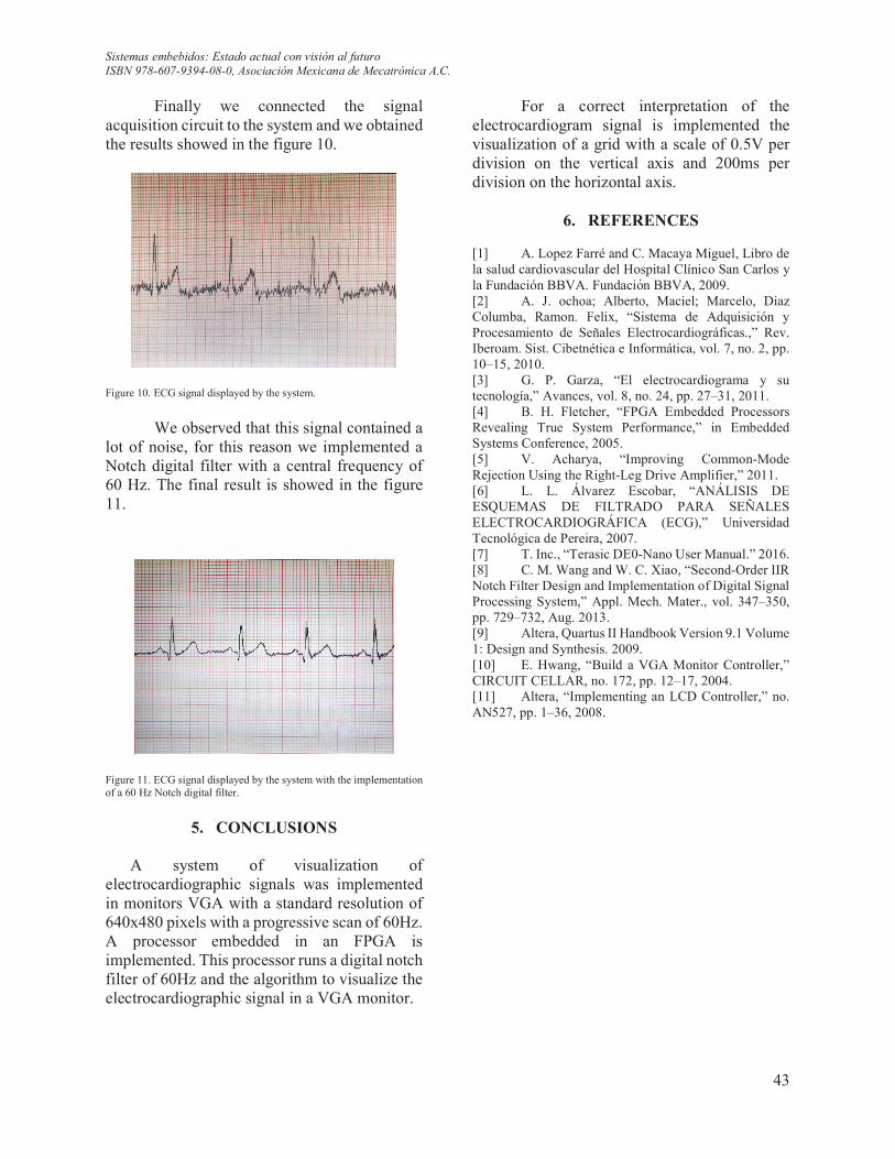
Sistemas embebidos: Estado actual con visión al futuro
ISBN 978-607-9394-08-0, Asociación Mexicana de Mecatrónica A.C.
43
Finally we connected the signal acquisition circuit to the system and we obtained the results showed in the figure 10.
Figure 10. ECG signal displayed by the system.
We observed that this signal contained a
lot of noise, for this reason we implemented a Notch digital filter with a central frequency of 60 Hz. The final result is showed in the figure 11.
Figure 11. ECG signal displayed by the system with the implementation of a 60 Hz Notch digital filter.
5. CONCLUSIONS
A system of visualization of
electrocardiographic signals was implemented in monitors VGA with a standard resolution of 640x480 pixels with a progressive scan of 60Hz. A processor embedded in an FPGA is implemented. This processor runs a digital notch filter of 60Hz and the algorithm to visualize the electrocardiographic signal in a VGA monitor.
For a correct interpretation of the electrocardiogram signal is implemented the visualization of a grid with a scale of 0.5V per division on the vertical axis and 200ms per division on the horizontal axis.
6. REFERENCES [1] A. Lopez Farré and C. Macaya Miguel, Libro de la salud cardiovascular del Hospital Clínico San Carlos y la Fundación BBVA. Fundacion BBVA, 2009. [2] A. J. ochoa; Alberto, Maciel; Marcelo, Diaz Columba, Ramon. Felix, “Sistema de Adquisición y Procesamiento de Señales Electrocardiográficas.,” Rev. Iberoam. Sist. Cibetnética e Informática, vol. 7, no. 2, pp. 10–15, 2010. [3] G. P. Garza, “El electrocardiograma y su tecnología,” Avances, vol. 8, no. 24, pp. 27–31, 2011. [4] B. H. Fletcher, “FPGA Embedded Processors Revealing True System Performance,” in Embedded Systems Conference, 2005. [5] V. Acharya, “Improving Common-Mode Rejection Using the Right-Leg Drive Amplifier,” 2011. [6] L. L. Álvarez Escobar, “ANÁLISIS DE ESQUEMAS DE FILTRADO PARA SEÑALES ELECTROCARDIOGRÁFICA (ECG),” Universidad Tecnológica de Pereira, 2007. [7] T. Inc., “Terasic DE0-Nano User Manual.” 2016. [8] C. M. Wang and W. C. Xiao, “Second-Order IIR Notch Filter Design and Implementation of Digital Signal Processing System,” Appl. Mech. Mater., vol. 347–350, pp. 729–732, Aug. 2013. [9] Altera, Quartus II Handbook Version 9.1 Volume 1: Design and Synthesis. 2009. [10] E. Hwang, “Build a VGA Monitor Controller,” CIRCUIT CELLAR, no. 172, pp. 12–17, 2004. [11] Altera, “Implementing an LCD Controller,” no. AN527, pp. 1–36, 2008.
Sistemas embebidos: Estado actual con visión al futuro
ISBN 978-607-9394-08-0, Asociación Mexicana de Mecatrónica A.C.
44
DISEÑO E IMPLEMENTACIÓN DE UN MONITOR DE VIDA SILVESTRE
SUSTENTABLE MEDIANTE RASPBERRY PI Omar Eduardo Ramírez Soto #1, Edwin Alberto Hernández Moreno#2, José Antonio Valentín Rodriguez#3, Jonathan
Villanueva Tavira *4, Jorge Salvador Valdez Martínez#5,, Verónica Sánchez López#6
# Universidad Tecnológica Emiliano Zapata del Estado de Morelos
Dirección Av. Universidad Tecnológica No.1, Col. Palo Escrito, C.P.62760, Emiliano Zapata, Morelos, México.
2 [email protected] [email protected]
Resumen—El presente artículo detalla el proyecto realizado en la Universidad Tecnológica Emiliano Zapata del Estado de Morelos (UTEZ) en la materia de Electrónica Digital. El proyecto consistió implementar un dispositivo capaz de realizar el monitoreo de las especies de animales que habitan el campus universitario. Lo anterior, debido a que actualmente se están realizando obras de ampliación con el objeto de dar mayor cobertura de educación a los jóvenes del estado de Morelos. Sin embargo, una problemática es que no se conoce en su totalidad el número de especies que habitan en los alrededores de la universidad, por consiguiente, se planteó el uso del sistema embebido Raspberry Pi para realizar esta labor. El objetivo de este proyecto consiste en recolectar información sobre la forma en que viven las distintas especies de animales que habitan en la universidad con el fin de ayudar a los ecologistas, biólogos, incluso científicos a recaudar la información necesaria para conocer el comportamiento y observar la invasión de la mancha urbana y las alteraciones en el ecosistema.
1. INTRODUCCIÓN
El estado de Morelos, por su situación geográfica y cambiante relieve, posee una gran variedad de áreas climáticas que determinan su riqueza biológica, debido a ello cuenta con una gran cantidad de
especies tanto de flora como de fauna. Morelos ocupa tan sólo el 0.25% del territorio mexicano y sin embargo, en él se registran en la actualidad el 21% de las especies de mamíferos mexicanos, el 33% de aves, el 14% de réptiles y el
10% de plantas vasculares reportadas para el país, por ello, Morelos se ubica en el lugar 17 con respecto a otros estados en cuanto a riqueza de especies, y además se encuentra entre los nueve estados con elevado endemismo de flora [1].
La biodiversidad de Morelos depende fundamentalmente de las condiciones ambientales prevalecientes dentro de su territorio, así como de su posición geográfica entre dos regiones consideradas como centros de endemismos: el Eje Neovolcánico y la Cuenca del Balsas [1]. En lo que respecta a la fauna de vertebrados silvestres las especies más importantes en el estado de Morelos, por su presencia, diversidad e intensidad de usos, son por orden de importancia las siguientes: el tejón, venado, víbora de cascabel, iguana, armadillo, coyote, zorrillo, tlacuache, ardilla, rata, huilota,
Sistemas embebidos: Estado actual con visión al futuro
ISBN 978-607-9394-08-0, Asociación Mexicana de Mecatrónica A.C.
45
zorra, gato montés y tuza. El conejo es la única especie con presencia en el 100% para todo el Estado, el tejón tlacuache y venado para las zonas sur y norte y víbora de cascabel para la zona centro y norte [1].
2. PROBLEMÁTICA El incremento de las actividades que
desarrollan los seres humanos cada día causa mayor impacto sobre los ecosistemas. Problemas como la deforestación, el cambio en el uso del suelo, los incendios forestales, la contaminación entre otros hace cada día más evidente la necesidad de emprender acciones concretas para resolver los problemas ambientales. Como parte de las actividades que permitan conservar el mayor número de animales que habitan en la universidad se han comenzado a realizar diversas acciones que permitan evaluar la sustentabilidad de la misma [1].
3. DISEÑO DEL MONITOR DE VIDA SILVESTRE
Tradicionalmente, el proceso de
grabación de los animales se realizaba de una forma manual, el cual consistía en esperar por largas jornadas de tiempo a que el animal realizara su aparición y de esta forma obtener algunas tomas de su comportamiento . Sin embargo, con la aparición del sistema embebido Raspberry Pi se puede realizar dicho monitoreo desde la comodidad de la computadora personal (Figura 1). Es importante mencionar que el proyecto proporciona también el valor de tres variables relacionadas con el ecosistema como: la temperatura, la humedad y la presión con el fin de relacionar la actividad de la fauna con los factores climáticos de la zona.
Figura1. Sistema embebido Raspberry Pi.
A continuación se describen cada una de
las partes que conforman el dispositivo realizado para lograr el monitoreo de las diversas especies de animales que habitan en el campus universitario.
a) Sistema Electrónico y Periféricos. – En lo que respecta al sistema electrónico, se emplea la tarjeta Raspberry Pi como unidad central de procesamiento. Es importante mencionar que variables adquiridas para este proyecto son: la temperatura, humedad y presión. Esta tarea es posible debido al uso de la tarjeta Sense HAT, y la RaspiCAM (Ver Figura 2).
Figura2. Tarjeta Sense HAT.
La tarjeta Sense HAT cuenta con un sensor de presión y de temperatura, con una resolución de 24 y 16 bits respectivamente [3].
La tarjeta Raspberry Pi 2B se utiliza para programar y ejecutar el código que se necesita cuando el sensor detecta la presencia de un animal, para esto se enviará una señal para activar la cámara, y
Sistemas embebidos: Estado actual con visión al futuro
ISBN 978-607-9394-08-0, Asociación Mexicana de Mecatrónica A.C.
46
que comience a grabar y/o a tomar fotos por un tiempo predeterminado. Adicionalmente, el módulo Sense HAT se utiliza para monitorear y registrar las distintas variables. b) Comunicaciones.- La comunicación
con el dispositivo se realiza a través del estándar 802.11b conocido como Wi-Fi. Esto se realiza por medio de un router y una dirección IP estática en la Raspberry Pi . De esta forma podemos ingresar a los recursos de la Raspberry Pi.
c) Sensores.- Los sensores con los que se equipa cada uno de los dispositivos son de tipo infrarrojos y están diseñados especialmente para la detección, de objetos incluso bajo condiciones ambientales extremas. Este componente puede tener la apariencia de un LED normal, la diferencia radica en que la luz emitida por él no es visible para el ojo humano, únicamente puede ser percibida por otros dispositivos electrónicos (Ver Figura 3).
Figura 3.- Sensor Infrarrojo empleado
d) Fuente de alimentación.- Una de las partes principales para el funcionamiento de este proyecto es sin duda alguna la energía que se le proporciona al mismo. Para este proyecto consideramos realizar la alimentación por medio de paneles solares con el objeto de utilizar a energía proveniente de la radiación solar. A continuación podemos
observar un diagrama a bloques del conjunto de elementos que interactúan para conformar nuestro dispositivo.
Figura 4. Estructura del Hardware de Dispositivo.
4. PRUEBAS Y RESULTADOS Finalmente, para probar el dispositivo
se ejecuta el archivo script que contiene el código de programación correspondiente implementado en el lenguaje de programación Python. Sin embargo, hasta el momento sólo es posible visualizar las operaciones desde la terminal de la Rasberry Pi, ya que por el momento no se cuenta con una interfaz gráfica amigable para monitorear los datos a distancia. Para las pruebas en campo se realizó el montaje de los diversos dispositivos en pequeñas casas de madera con alimento como semillas y fruta con el objeto de atraer de una mejor forma a la fauna que vive en el campus de la Universidad. (Ver Figura 5).
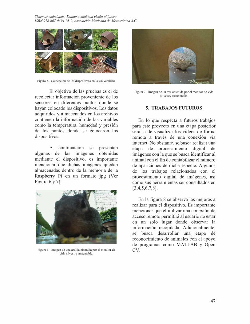
Sistemas embebidos: Estado actual con visión al futuro
ISBN 978-607-9394-08-0, Asociación Mexicana de Mecatrónica A.C.
47
Figura 5.- Colocación de los dispositivos en la Universidad.
El objetivo de las pruebas es el de recolectar información proveniente de los sensores en diferentes puntos donde se hayan colocado los dispositivos. Los datos adquiridos y almacenados en los archivos contienen la información de las variables como la temperatura, humedad y presión de los puntos donde se colocaron los dispositivos.
A continuación se presentan algunas de las imágenes obtenidas mediante el dispositivo, es importante mencionar que dichas imágenes quedan almacenadas dentro de la memoria de la Raspberry Pi en un formato jpg (Ver Figura 6 y 7).
Figura 6.- Imagen de una ardilla obtenida por el monitor de vida silvestre sustentable.
Figura 7.- Imagen de un ave obtenida por el monitor de vida silvestre sustentable.
5. TRABAJOS FUTUROS En lo que respecta a futuros trabajos
para este proyecto en una etapa posterior será la de visualizar los videos de forma remota a través de una conexión vía internet. No obstante, se busca realizar una etapa de procesamiento digital de imágenes con la que se busca identificar al animal con el fin de contabilizar el número de apariciones de dicha especie. Algunos de los trabajos relacionados con el procesamiento digital de imágenes, así como sus herramientas ser consultados en [3,4,5,6,7,8].
En la figura 8 se observa las mejoras a
realizar para el dispositivo. Es importante mencionar que el utilizar una conexión de acceso remoto permitirá al usuario no estar en un solo lugar donde observar la información recopilada. Adicionalmente, se busca desarrollar una etapa de reconocimiento de animales con el apoyo de programas como MATLAB y Open CV.
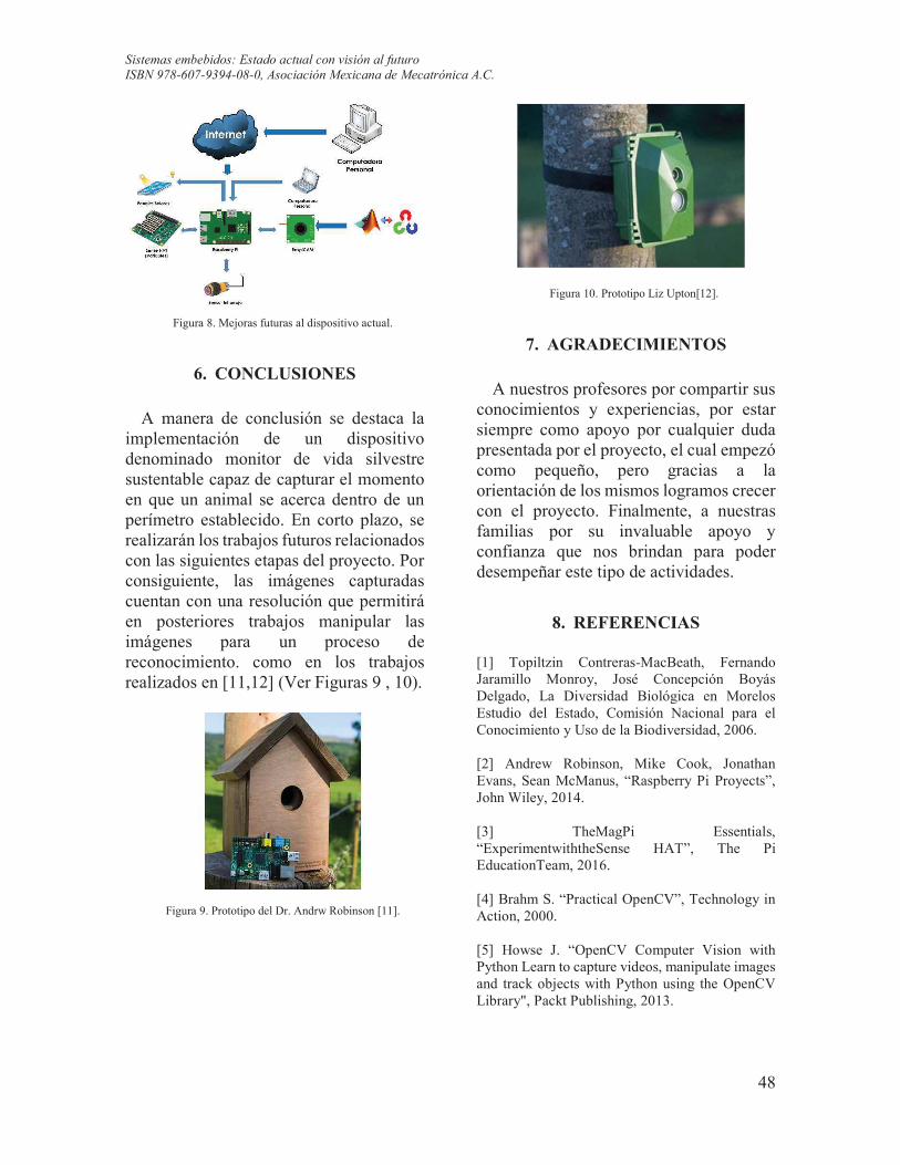
Sistemas embebidos: Estado actual con visión al futuro
ISBN 978-607-9394-08-0, Asociación Mexicana de Mecatrónica A.C.
48
Figura 8. Mejoras futuras al dispositivo actual.
6. CONCLUSIONES A manera de conclusión se destaca la
implementación de un dispositivo denominado monitor de vida silvestre sustentable capaz de capturar el momento en que un animal se acerca dentro de un perímetro establecido. En corto plazo, se realizarán los trabajos futuros relacionados con las siguientes etapas del proyecto. Por consiguiente, las imágenes capturadas cuentan con una resolución que permitirá en posteriores trabajos manipular las imágenes para un proceso de reconocimiento. como en los trabajos realizados en [11,12] (Ver Figuras 9 , 10).
Figura 9. Prototipo del Dr. Andrw Robinson [11].
Figura 10. Prototipo Liz Upton[12].
7. AGRADECIMIENTOS A nuestros profesores por compartir sus
conocimientos y experiencias, por estar siempre como apoyo por cualquier duda presentada por el proyecto, el cual empezó como pequeño, pero gracias a la orientación de los mismos logramos crecer con el proyecto. Finalmente, a nuestras familias por su invaluable apoyo y confianza que nos brindan para poder desempeñar este tipo de actividades.
8. REFERENCIAS [1] Topiltzin Contreras-MacBeath, Fernando Jaramillo Monroy, José Concepción Boyás Delgado, La Diversidad Biológica en Morelos Estudio del Estado, Comisión Nacional para el Conocimiento y Uso de la Biodiversidad, 2006. [2] Andrew Robinson, Mike Cook, Jonathan Evans, Sean McManus, “Raspberry Pi Proyects”, John Wiley, 2014. [3] TheMagPi Essentials, “ExperimentwiththeSense HAT”, The Pi EducationTeam, 2016. [4] Brahm S. “Practical OpenCV”, Technology in Action, 2000.
[5] Howse J. “OpenCV Computer Vision with Python Learn to capture videos, manipulate images and track objects with Python using the OpenCV Library", Packt Publishing, 2013.
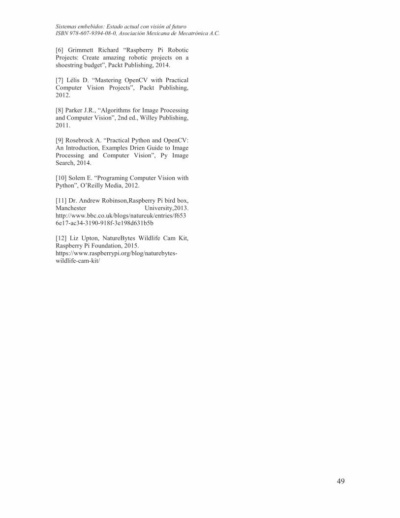
Sistemas embebidos: Estado actual con visión al futuro
ISBN 978-607-9394-08-0, Asociación Mexicana de Mecatrónica A.C.
49
[6] Grimmett Richard “Raspberry Pi Robotic Projects: Create amazing robotic projects on a shoestring budget”, Packt Publishing, 2014. [7] Lélis D. “Mastering OpenCV with Practical Computer Vision Projects”, Packt Publishing, 2012.
[8] Parker J.R., “Algorithms for Image Processing and Computer Vision”, 2nd ed., Willey Publishing, 2011. [9] Rosebrock A. “Practical Python and OpenCV: An Introduction, Examples Drien Guide to Image Processing and Computer Vision”, Py Image Search, 2014. [10] Solem E. “Programing Computer Vision with Python”, O’Reilly Media, 2012. [11] Dr. Andrew Robinson,Raspberry Pi bird box, Manchester University,2013. http://www.bbc.co.uk/blogs/natureuk/entries/f6536e17-ac34-3190-918f-3e198d631b5b [12] Liz Upton, NatureBytes Wildlife Cam Kit, Raspberry Pi Foundation, 2015. https://www.raspberrypi.org/blog/naturebytes-wildlife-cam-kit/

50
Fe de errata
Por omisión del comité editorial, se incluye un capítulo en la presente obra que de forma involuntaria no se incluyo en la impresión original.
Sistemas embebidos: Estado actual con visión al futuro
ISBN 978-607-9394-08-0, Asociación Mexicana de Mecatrónica A.C.
51
TUNABLE OPTICAL FILTER BASED ON ELONGATION CONTROL
J. A. Mejía-Islas, G. G. Pérez-Sánchez*a, A. Gómez-Vieyraa, J. R Pérez-Torresb
aUniversidad Autónoma Metropolitana, Av. San Pablo 180, Reynosa Tamaulipas, Azc. México City 02200.
bTecnológico de Estudios Superiores de Coacalco, Av. 16 de Septiembre 54, Cabecera Municipal, Coacalco de Berriozábal, México 55700.
Corresponding´s Author e-mail: [email protected]
ABSTRACT
Abstract— The present work shows the prototype design and the control system results of a tunable optical filter based on a fiber Bragg grating and an elongation control system. As a first stage the optical characterization of the optical filter was made, then the stepper motors were selected for the desired wavelength selection with a couple of pulleys which produce the grating elongation and as a consequence the wavelength shifting, the pulleys diameters were calculated for produce 0.08 nm shift for each motor step finally the control program was introduced for selecting the desired filtering wavelength.
Keywords: Optical Filter, Bragg Gratings, Tunable Filter, Elongation Control System.
1. INTRODUCTION
Optical communications systems as well as research and teaching areas, have both the need to have tunable optical filters. The former to be able to select different wavelengths that are transferred in the same transmission medium, and the latter require devices with a large dynamic range that allow to explore of effects at different wavelengths.
Existing tunable filters base their operation on thermal processes or
nonlinearities that require a high degree of signal control. However, the current requirements present the need to have simple control signal tuning alternatives, easy implementation and low cost. An alternative is to employ the fiber optic filters.
Fiber optic filters are devices that allow the elimination of certain wavelengths transmitted in a fiber optic. Such devices are highly used in both fiber optic communications networks, and in fiber optic testing and monitoring systems as sensors. The main applications of optical filters in optical communication systems include: Elimination of noise, introduced, for example, by optical amplifiers; equalization of the response of optical amplifiers, election of channels in WDM systems.
In order to perform these applications optimally they must have low insertion losses. Ideally, their passband must be flat to avoid signal distortion. The transition band of their response must be abrupt to avoid cross-talk with the neighboring channels and it is also necessary that its behavior is independent of the polarization of the signal.
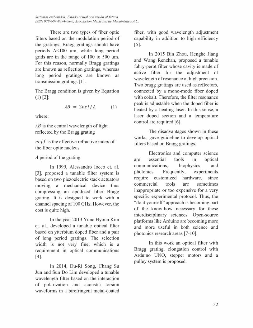
Sistemas embebidos: Estado actual con visión al futuro
ISBN 978-607-9394-08-0, Asociación Mexicana de Mecatrónica A.C.
52
There are two types of fiber optic filters based on the modulation period of the gratings. Bragg gratings should have periods Λ<100 μm, while long period grids are in the range of 100 to 500 μm. For this reason, normally Bragg gratings are known as reflection gratings, whereas long period gratings are known as transmission gratings [1].
The Bragg condition is given by Equation (1) [2]:
ÍÎ ! 29���Ï (1)
where:
ÍÎ is the central wavelength of light reflected by the Bragg grating
9��� is the effective refractive index of the fiber optic nucleus
Ï period of the grating.
In 1999, Alessandro Iocco et. al. [3], proposed a tunable filter system is based on two piezoelectric stack actuators moving a mechanical device thus compressing an apodized fiber Bragg grating. It is designed to work with a channel spacing of 100 GHz. However, the cost is quite high.
In the year 2013 Yune Hyoun Kim et. al., developed a tunable optical filter based on ytterbium doped fiber and a pair of long period gratings. The selection width is not very fine, which is a requirement in optical communications [4].
In 2014, Du-Ri Song, Chang Su Jun and Sun Do Lim developed a tunable wavelength filter based on the interaction of polarization and acoustic torsion waveforms in a birefringent metal-coated
fiber, with good wavelength adjustment capability in addition to high efficiency [5].
In 2015 Bin Zhou, Henghe Jiang and Wang Renzhan, proposed a tunable fabry-perot filter whose cavity is made of active fiber for the adjustment of wavelength of resonance of high precision. Two bragg gratings are used as reflectors, connected by a mono-mode fiber doped with cobalt. Therefore, the filter resonance peak is adjustable when the doped fiber is heated by a heating laser. In this sense, a laser doped section and a temperature control are required [6].
The disadvantages shown in these works, gave guideline to develop optical filters based on Bragg gratings.
Electronics and computer science are essential tools in optical communications, biophysics and photonics. Frequently, experiments require customized hardware, since commercial tools are sometimes inappropriate or too expensive for a very specific experimental protocol. Thus, the “do it yourself” approach is becoming part of the know-how necessary for these interdisciplinary sciences. Open-source platforms like Arduino are becoming more and more useful in both science and photonics research areas [7-10].
In this work an optical filter with Bragg grating, elongation control with Arduino UNO, stepper motors and a pulley system is proposed.
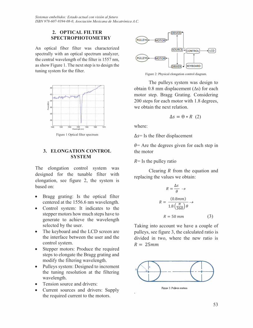
Sistemas embebidos: Estado actual con visión al futuro
ISBN 978-607-9394-08-0, Asociación Mexicana de Mecatrónica A.C.
53
2. OPTICAL FILTER SPECTROPHOTOMETRY
An optical fiber filter was characterized spectrally with an optical spectrum analyzer, the central wavelength of the filter is 1557 nm, as show Figure 1. The next step is to design the tuning system for the filter.
Figure 1 Optical filter spectrum
3. ELONGATION CONTROL SYSTEM
The elongation control system was designed for the tunable filter with elongation, see figure 2, the system is based on:
· Bragg grating: Is the optical filter centered at the 1556.6 nm wavelength.
· Control system: It indicates to the stepper motors how much steps have to generate to achieve the wavelength selected by the user.
· The keyboard and the LCD screen are the interface between the user and the control system.
· Stepper motors: Produce the required steps to elongate the Bragg grating and modify the filtering wavelength.
· Pulleys system: Designed to increment the tuning resolution at the filtering wavelength.
· Tension source and drivers: · Current sources and drivers: Supply
the required current to the motors.
Figure 2: Physical elongation control diagram.
The pulleys system was design to obtain 0.8 mm displacement (∆s) for each motor step. Bragg Grating. Considering 200 steps for each motor with 1.8 degrees, we obtain the next relation.
∆0 ! Ɵ ∗ - (2)
where:
∆0= Is the fiber displacement
+= Are the degrees given for each step in the motor
-= Is the pulley ratio
Clearing - from the equation and replacing the values we obtain:
- ! ∆0 + ® - ! H0.8RRJ
1.8 Ò Ó360Õ +®
- ! 50 RR (3)
Taking into account we have a couple of pulleys, see figure 3, the calculated ratio is divided in two, where the new ratio is - ! 25RR
.
Sistemas embebidos: Estado actual con visión al futuro
ISBN 978-607-9394-08-0, Asociación Mexicana de Mecatrónica A.C.
54
In figure 4 the flow diagram of the program used for the stepper motors control is shown, which the desired filtering wavelength will be achieved.
Figure 4. Flow diagram for the elongation control system.
The Arduino’s program [11] which a 0.8 mm of displacement in the Bragg grating is guaranteed, presented below
/* ----------------------------------------------------------------
ONE BRAGG GRATING ELONGATION CONTROL
PROGRAM
*/
//REQUIRED LIBRARIES
#include <Keypad.h>// keyboard library
#include <Wire.h>// I2C screen library
#include <LiquidCrystal_I2C.h>//LCD I2 library
LiquidCrystal_I2C lcd(0x27,20,4);
//-----------KEYBOARD CONFIGURATION
const byte Filas = 4; //four rows
const byte Cols = 3; //four columns
byte Pins_Filas[] = {8, 7, 6, 5}; // Arduino’s Pines where the
rows are counted
byte Pins_Cols[] = { 4, 3, 2}; // Arduino’s Pines where the
columns are counted
char Teclas [ Filas ][ Cols ] =
{
{'1','2','3'},
{'4','5','6'},
{'7','8','9'},
{'*','0','#'}
};
Keypad Teclado1 = Keypad(makeKeymap(Teclas), Pins_Filas,
Pins_Cols, Filas, Cols);
//----------------------VARIABLES AND CONSTANTS
int q =1; //____ lock variable
int referencia=0; //____ lock variable
int n = 0; //____ lock variable
#define STEP 12 //____ Pin 12 for step
#define DIR 13 //____ Pin 13 for dir
#define botton 11
#define botton2 10
void setup()
{
//____________________MOTORS
STARTING______________________
pinMode(DIR,OUTPUT); //Output pines
pinMode(STEP,OUTPUT); //Output pines
pinMode (botton,INPUT); //Input pines
pinMode (botton2,INPUT); //Input pines
digitalWrite(DIR, LOW); //
digitalWrite(STEP,LOW);
//________SCREEN
lcd.backlight();
lcd.init(); //screen starting
lcd.setCursor(5,1);
lcd.print("Bienvenidos"); // welcome message
delay (3000); /// 3s delay
}
void loop()
{ char pulsación = Teclado1.getKey() ; //input key
capture
if (pulsación == NO_KEY &&q ==1) // If
value= 0 non key has been pressured
{
menu_inicial (); // call to menu_inicial function
}
switch (pulsacion) // switch structure for matricial
keyboard
{
case '*':
menu_inicial ();
break;
case '1':
if (q==0)
n=1;
activar_motor (); //______Call to activar motor function
break;
case '2':
if (q==0)
n=2;
activar_motor ();
break;
case '3':
if (q==0)
n=3;
activar_motor ();
break;
case '4':
if (q==0)
n=4;
activar_motor ();
Sistemas embebidos: Estado actual con visión al futuro
ISBN 978-607-9394-08-0, Asociación Mexicana de Mecatrónica A.C.
55
break;
case '5':
if (q==0)
n=5;
activar_motor ();
break;
case '6':
if (q==0)
n=6;
activar_motor ();
break;
case '7':
if (q==0)
n=7;
activar_motor ();
break;
case '8':
if (q==0)
n=8;
activar_motor ();
break;
case '9':
if (q==0)
n=9;
activar_motor ();
break;
}
}
_____________PROGRAM FUNCTIONS__________
//(1)
void activar_motor()
{
lcd.clear(); //Clear LCD
lcd.print("corgando....."); // loading selected option
if (referencia <1600){ // Lock to avoid fiber rupture
digitalWrite(DIR,HIGH); //direction fixed
//for (int a=0; a < n; a++){ //n= step numbers
for(int i=0;i<n;i++){ // Send 10 pulses to the motor
digitalWrite(STEP,HIGH); //time pulse 5ms
delay(5);
digitalWrite(STEP,LOW);
delay(5);
referencia=referencia + 1;
q=2; //lock variable
}
}
}
//(2)
void menu_inicial()
{
q=0;
lcd.clear();//clear LCD
if (referencia != 0 ){
digitalWrite(DIR,LOW); //Change turning sense
for(int i=0;i<n;i++){ // 2000 steps in the opposite sense
digitalWrite(STEP,HIGH);
delay(5);
digitalWrite(STEP,LOW);
delay(5);
referencia = referencia - 1;
}
}
else{
digitalWrite(STEP,LOW);
}
lcd.print("ELIJE UNA LONGUITUD");//To write in the first
line
lcd.setCursor(0,1);//Jump to the second line
lcd.print("1=XXXX 2=XXXX 3=XXXX");// To write in the
second line
lcd.setCursor(0,2);// Jump to the third line
lcd.print("4=XXXX 5=XXXX 6=XXXX");// To write in the
third line
lcd.setCursor(0,3);//Jump to the fourth
lcd.print("7=XXXX 8=XXXX 9=XXXX");// To write in the
fourth line
}
Figure 5 shows the tunable optical filter prototype with the elongation control designed in the Universidad Autónoma Metropolitana-Azcapotzalco.
Figure 5. Tunable optical filter prototype.
Figure 6 shows the wavelength displacement generated by 1 step with the elongation system, where it is clear the shift to higher wavelengths obtaining a tunable filter.
Figure 6. Tunable filter wavelength.
Sistemas embebidos: Estado actual con visión al futuro
ISBN 978-607-9394-08-0, Asociación Mexicana de Mecatrónica A.C.
56
4. CONCLUSIONS
This work presents the development of a prototype of a tunable optical filter which governs its operation in elongation control over the optical filter. The resolution of the device is 0.8 mm which is equivalent to 0.08 nm of displacement of the wavelength, which makes it Ideal for use in optical communications systems as it complies with ITU-T gratings.
Such device has the advantage of low cost and easy implementation. The current system can improve the resolution by changing the pulley system. The dynamic range of the device is 30 steps.
5. REFERENCES
[1] Kashyap, R. “Fiber Bragg gratings” USA: Elsevier Academic Press 2010.
[2] H. Arellano-Sotelo “Aplicación de las rejillas
de Bragg en fibra óptica para medición de
vibraciones en eventos de baja frecuencia”, M.Sc. thesis, Centro de Investigaciones en Óptica AC, Mexico 2006.
[3] A. Iocco, H. G. Limberger, R. P. Salathe, L. A. Everall, K. E. Chisholm, J. A. R. Williams, and I. Bennion, "Bragg Grating Fast Tunable Filter for
Wavelength Division Multiplexing". J. Lightwave
Technol. Vo. 17/1999, pp. 1217- 1221. Available:
https://www.osapublishing.org/jlt/abstract.cfm?ur
i=jlt-17-7-1217
[4] Y. H. Kim et al., "All-optical tunable comb
filters using ytterbium doped fibers and an LPG
pair", 18th OptoElectronics and Communications Conference held jointly with International Conference on Photonics in Switching (OECC/PS), 2013, pp. 1-2.
[5] D. r. Song et al., "Acousto-optic tunable filter
using torsional wave and metal coated birefringent
optical fiber" OptoElectronics and Communication Conference and Australian Conference on Optical Fibre Technology (OECC/ACOFT),2014, pp. 714-715.
[6] B. Zhou, H. Jiang, R. Wang and C. Lu, "Optical
Fiber Fiber Fabry–Perot Filter With Tunable
Cavity for High-Precision Resonance Wavelength
Adjustment”. J. of Lightwave Technol, vol. 33/2015, pp. 2950-2954. Aviable: http://ieeexplore.ieee.org/document/7094221/
[7] A. D’Ausilio, “Arduino: a low-cost
multipurpose lab equipment”. Behav. Res. Methods 44/2012, pp. 305–313 doi:10.3758/s13428-011-0163-z
[8] A. P. Ana et al., “BITalino: a biosignal
acquisition system based on Arduino,” Proceeding of the 6th Conference on Biometical Electronicsand Devices (BIODEVICES) 2013.
[9] J. A. Kornuta, M. E. Nipper, and J. B. Dixon, “Low-cost microcontroller platform for studying
lymphatic biomechanics in vitro”. J. Biomech, vol. 46/2013, pp. 183–186. doi: 10.1016/j.jbiomech.2012.09.031.
[10] A. Sierra-Calderon, J. C. Rodriguez-Novelo, E. Gamez-Aviles, M May-Alarcon, H. Toral-Cruz, J. A. Álvarez-Chávez, E. A. Andrade-González, J. R. Pérez-Torres, "Optimization and thermal ASE
noise, characterization of an all-fiber Sagnac
interferometer via LAN for sensing applications", in Infrared Sensors, Devices, and Applications VI, Paul D. LeVan; Ashok K. Sood; Priyalal S. Wijewarnasuriya; Arvind I. D'Souza, Editors, Proceedings of SPIE Vol. 9974, 2016, pp 99740W_1-8.
[11] Tojeiro G. “Taller de Arduino” España: Alfaomega Marcombo 2015.

Sistemas embebidos: Estado actual con visión al futuro
ISBN 978-607-9394-08-0, Asociación Mexicana de Mecatrónica A.C.
58
Sistemas embebidos: Estado actual con visión al futuro
Asociación Mexicana de Mecatrónica A.C. Prolongación Corregidora Norte No. 168, Interior E
Col. El Cerrito, C.P. 76160, Querétaro, Qro. Se tiraron 500 ejemplares, en formato digital pdf, tipo CD
Tamaño 80 Mb.
ISBN 978-607-9394-08-0,
Sistemas embebidos: Estado actual con visión al futuro
ISBN 978-607-9394-08-0, Asociación Mexicana de Mecatrónica A.C.
59