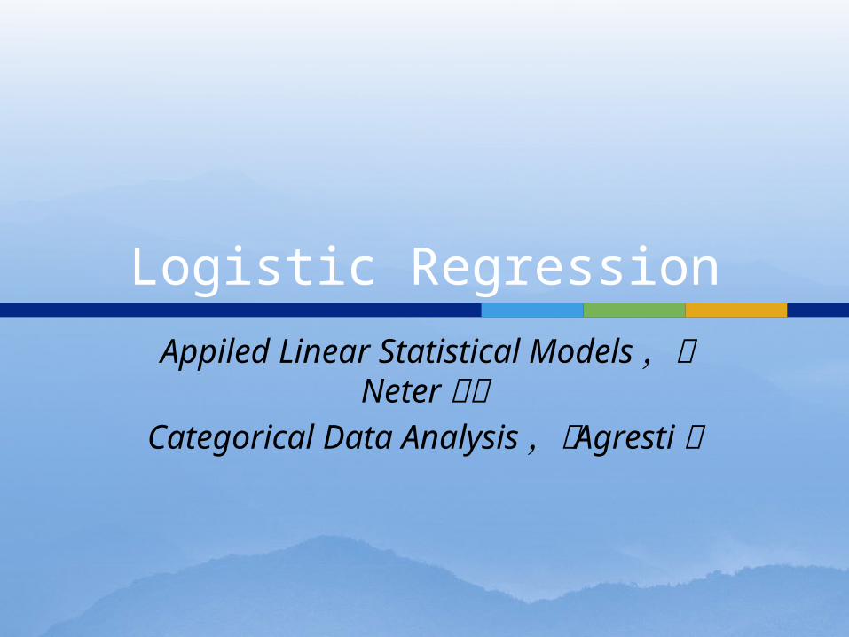
Logistic RegressionAppiled Linear Statistical

Models ，由 Neter 等著Categorical Data Analysis ，由

Agresti 著

当响应变量是定性变量时的非线性模型 两种可能的结果，成功或失败，患病的或没 有患病的，出席的或缺席的 实例： CAD( 心血管疾病 ) 是年龄，体重，性别，吸烟历史，血压的函数 吸烟者或不吸烟者是家庭历史，同年龄组行 为，收入，年龄的函数 今年购买一辆汽车是收入，当前汽车的使用 年限，年龄的函数

Logistic 回归

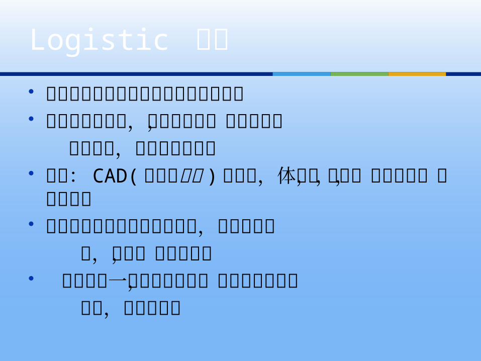
二元结果的响应函数

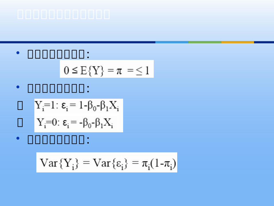
对响应函数的约束： 非标准化的误差项：当当 非恒量的误差方差：

当响应是二元时的特殊问题

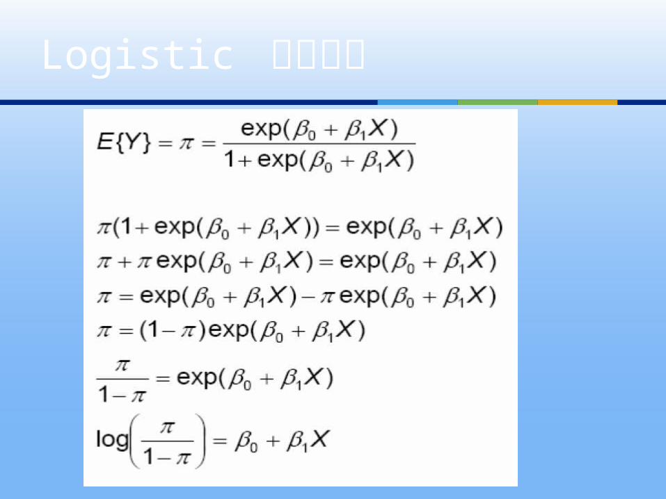
Logistic 响应函数

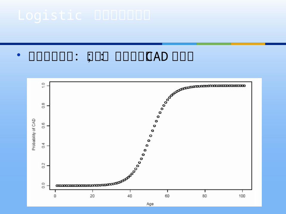
图中横坐标为：年龄；纵坐标为： CAD 的概率

Logistic 响应函数的例子

Logistic 响应函数的性质

似然函数

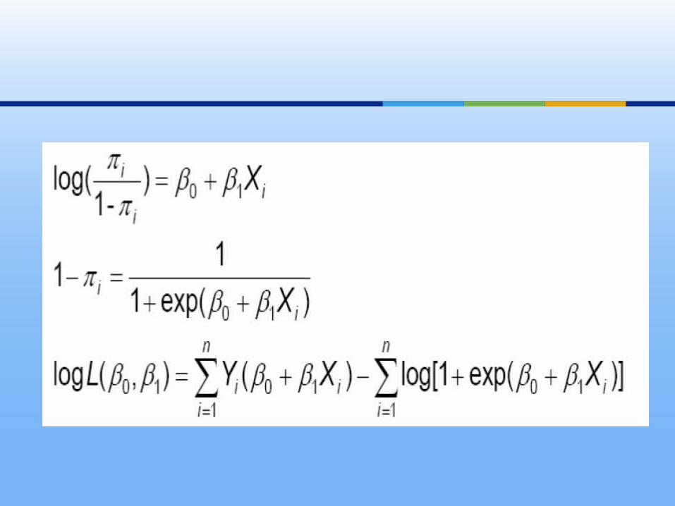
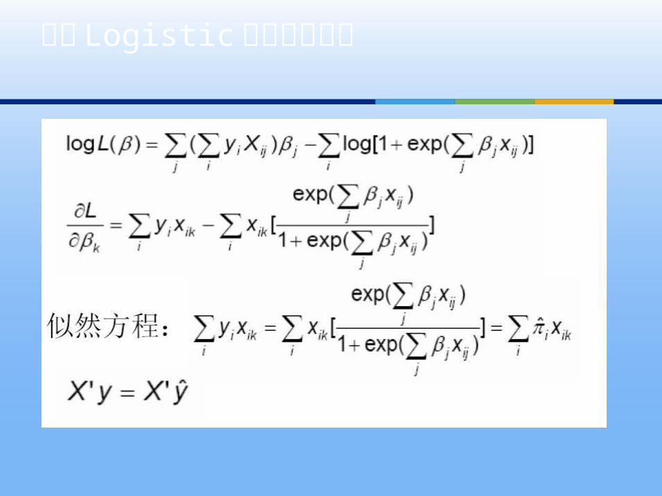
多元 Logistic 回归的似然性

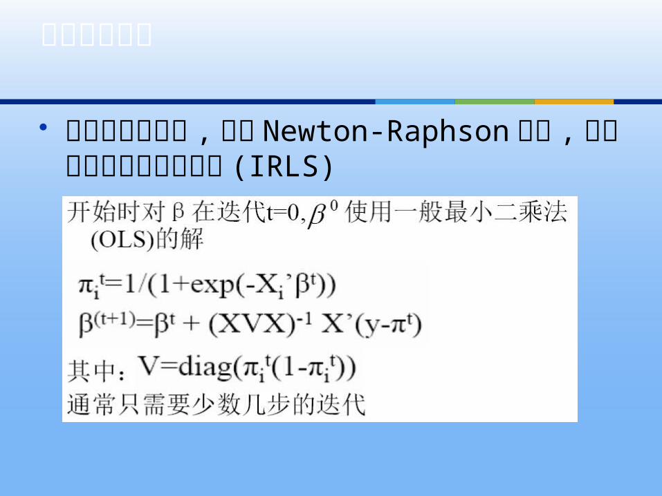
不封闭的形式解 , 使用 Newton-Raphson算法 , 迭代地重加权最小二乘法 (IRLS)

似然方程的解

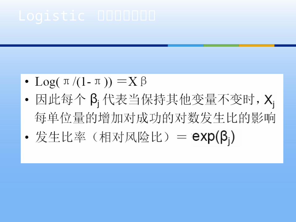
Logistic 回归系数的解释

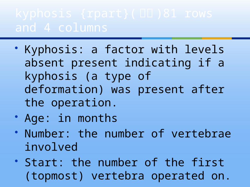
Kyphosis: a factor with levels absent present indicating if a kyphosis (a type of deformation) was present after the operation.

Age: in months Number: the number of vertebrae

involved Start: the number of the first

(topmost) vertebra operated on.

kyphosis {rpart}( 驼背 )81 rows and 4 columns

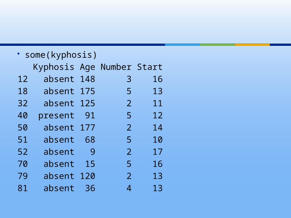
some(kyphosis) Kyphosis Age Number Start12 absent 148 3 1618 absent 175 5 1332 absent 125 2 1140 present 91 5 1250 absent 177 2 1451 absent 68 5 1052 absent 9 2 1770 absent 15 5 1679 absent 120 2 1381 absent 36 4 13

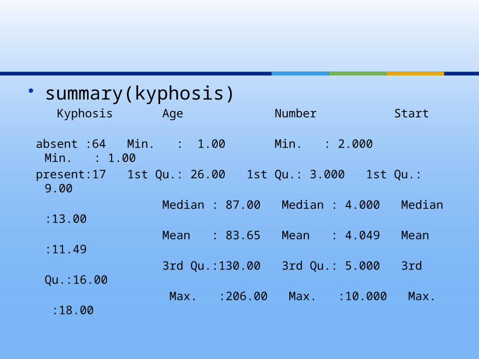
summary(kyphosis) Kyphosis Age Number Start absent :64 Min. : 1.00 Min. : 2.000 Min. : 1.00 present:17 1st Qu.: 26.00 1st Qu.: 3.000 1st Qu.: 9.00 Median : 87.00 Median : 4.000 Median :13.00 Mean : 83.65 Mean : 4.049 Mean :11.49 3rd Qu.:130.00 3rd Qu.: 5.000 3rd Qu.:16.00 Max. :206.00 Max. :10.000 Max. :18.00

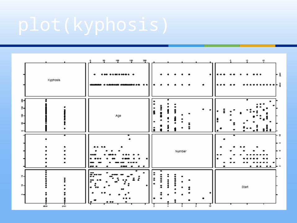
plot(kyphosis)

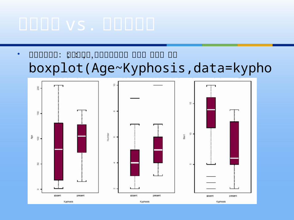
图中横坐标为：是否驼背；纵坐标分别为：年龄，数值，起始boxplot(Age~Kyphosis,data=kyphosis)

预测因子 vs. 驼背的箱图

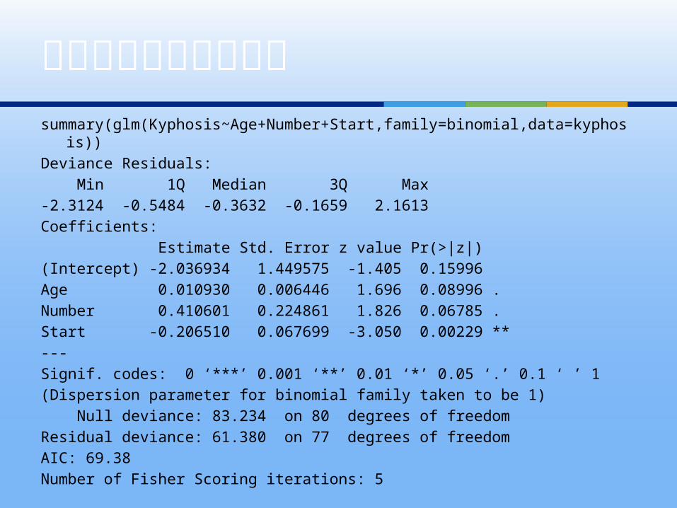
summary(glm(Kyphosis~Age+Number+Start,family=binomial,data=kyphosis))

Deviance Residuals: Min 1Q Median 3Q Max -2.3124 -0.5484 -0.3632 -0.1659 2.1613 Coefficients: Estimate Std. Error z value Pr(>|z|) (Intercept) -2.036934 1.449575 -1.405 0.15996 Age 0.010930 0.006446 1.696 0.08996 . Number 0.410601 0.224861 1.826 0.06785 . Start -0.206510 0.067699 -3.050 0.00229 **---Signif. codes: 0 ‘***’ 0.001 ‘**’ 0.01 ‘*’ 0.05 ‘.’ 0.1 ‘ ’ 1(Dispersion parameter for binomial family taken to be 1) Null deviance: 83.234 on 80 degrees of freedomResidual deviance: 61.380 on 77 degrees of freedomAIC: 69.38Number of Fisher Scoring iterations: 5

广义拉格朗日乘子拟合

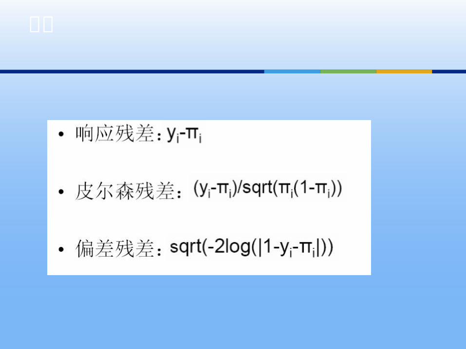
残差

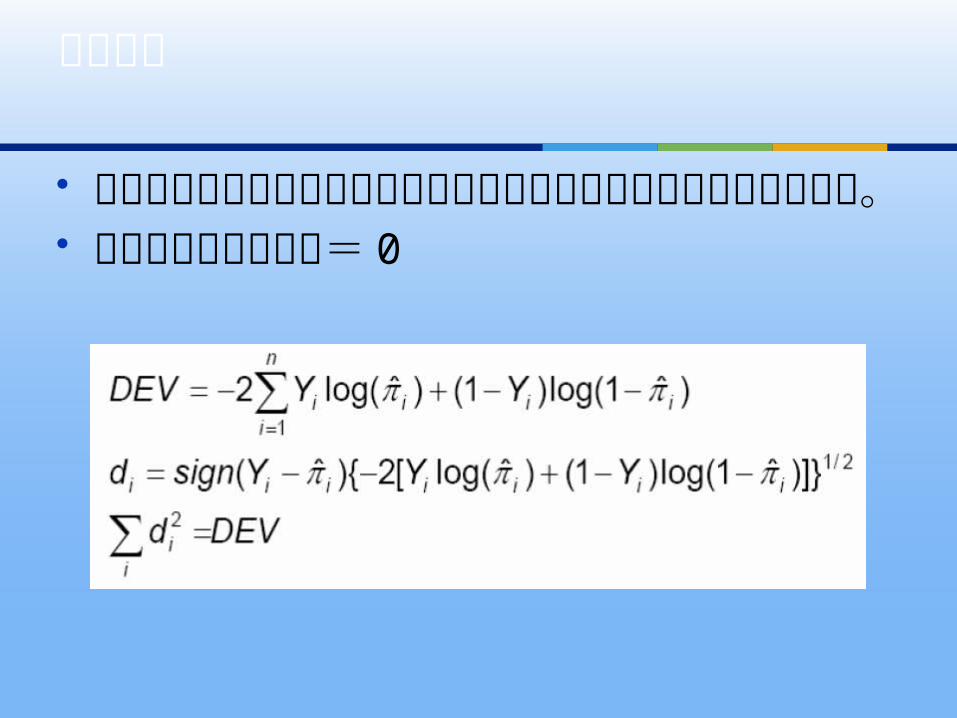
拟合模型的偏差是拟合模型的对数似然与饱和模型的对数似然的比值。 饱和模型的对数似然＝ 0

模型偏差

x<-model.matrix(kyph.glm) fi=fitted(kyph.glm) xvx<-t(x)%*%diag(fi*(1-fi))%*%x xvx (Intercept) Age Number Start(Intercept) 9.62034 907.8886 43.67401 86.49843Age 907.88858 114049.8138 3904.31285

9013.14288Number 43.67401 3904.3128 219.95349 378.82840Start 86.49843 9013.1429 378.82840 1024.07295

协方差矩阵

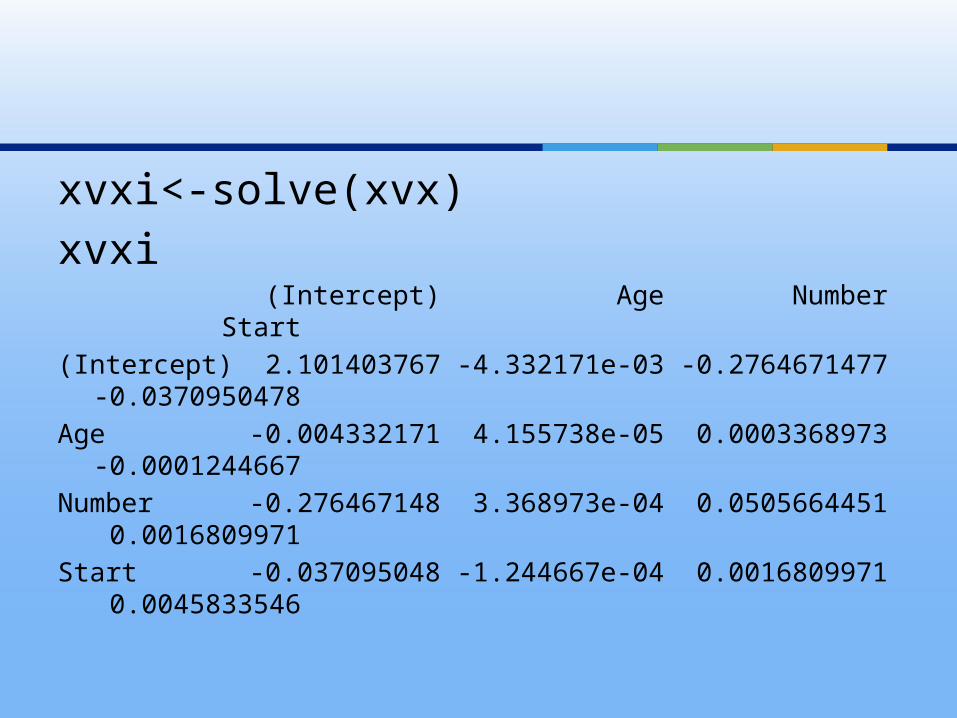
xvxi<-solve(xvx)xvxi (Intercept) Age Number Start(Intercept) 2.101403767 -4.332171e-03 -0.2764671477 -

0.0370950478Age -0.004332171 4.155738e-05 0.0003368973 -

0.0001244667Number -0.276467148 3.368973e-04 0.0505664451

0.0016809971Start -0.037095048 -1.244667e-04 0.0016809971

0.0045833546

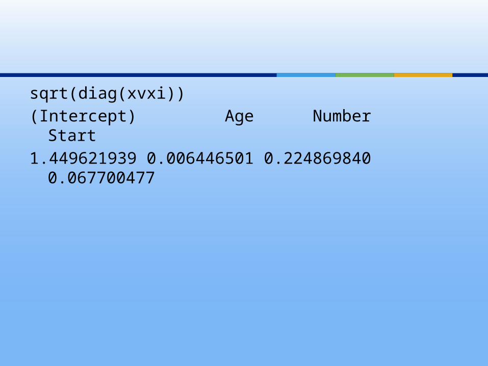
sqrt(diag(xvxi))(Intercept) Age Number Start 1.449621939 0.006446501 0.224869840

0.067700477

anova(kyph.glm)Analysis of Deviance Table

Model: binomial, link: logit

Response: Kyphosis

Terms added sequentially (first to last)

Df Deviance Resid. Df Resid. DevNULL 80 83.234Age 1 1.302 79 81.932Number 1 10.306 78 71.627Start 1 10.247 77 61.380

因向模型中增加项而产生的偏差变化

kyph.glm2<-glm(Kyphosis~poly(Age,2)+Number+Start,family=binomial,data=kyphosis)

summary(kyph.glm2)

带有附加的年龄 ^2 的驼背模型

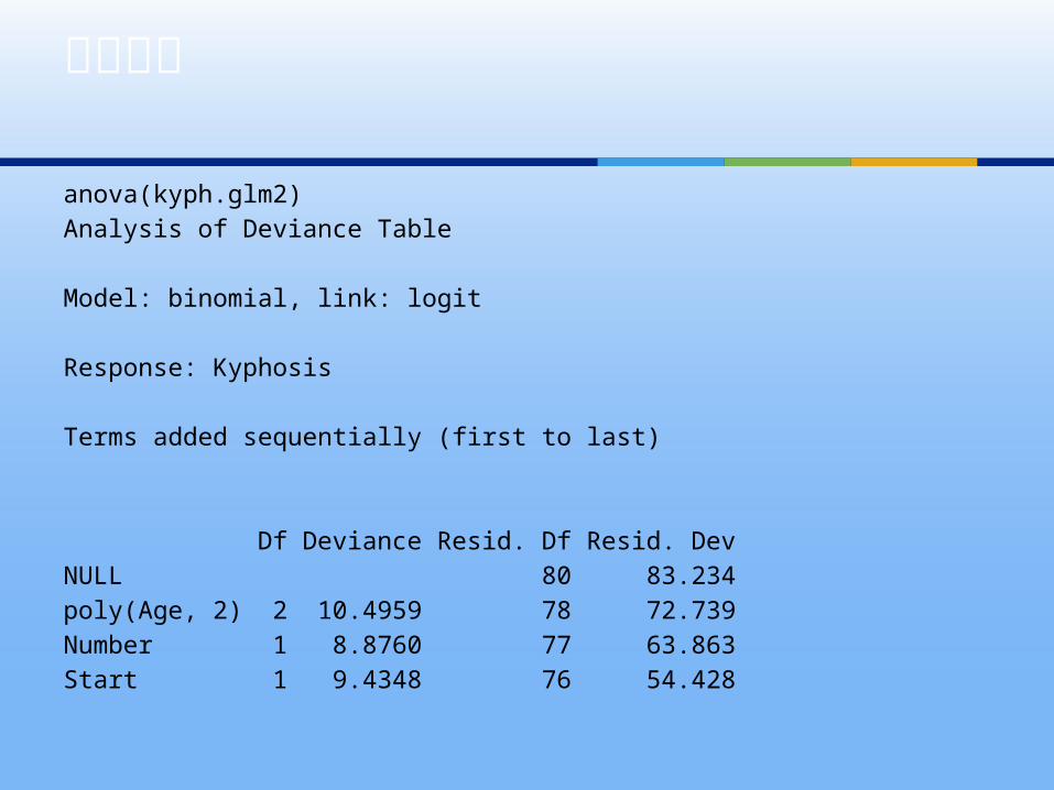
anova(kyph.glm2)Analysis of Deviance Table

Model: binomial, link: logit

Response: Kyphosis

Terms added sequentially (first to last)

Df Deviance Resid. Df Resid. DevNULL 80 83.234poly(Age, 2) 2 10.4959 78 72.739Number 1 8.8760 77 63.863Start 1 9.4348 76 54.428

偏差分析

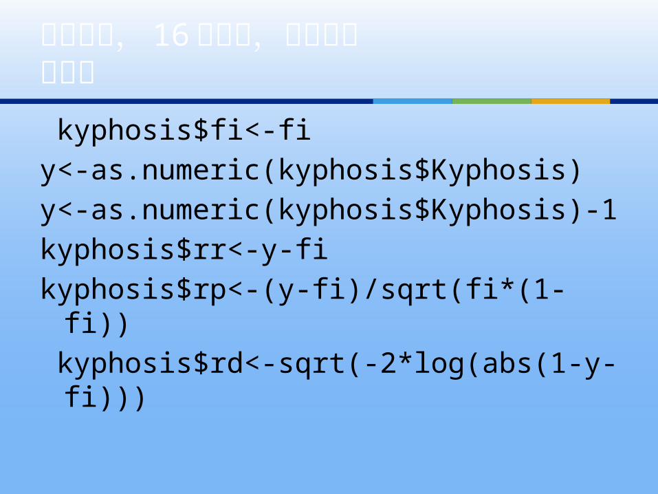
kyphosis$fi<-fiy<-as.numeric(kyphosis$Kyphosis)y<-as.numeric(kyphosis$Kyphosis)-1kyphosis$rr<-y-fikyphosis$rp<-(y-fi)/sqrt(fi*(1-fi)) kyphosis$rd<-sqrt(-2*log(abs(1-y-fi)))

驼背数据， 16 个对象，带有拟合和残差

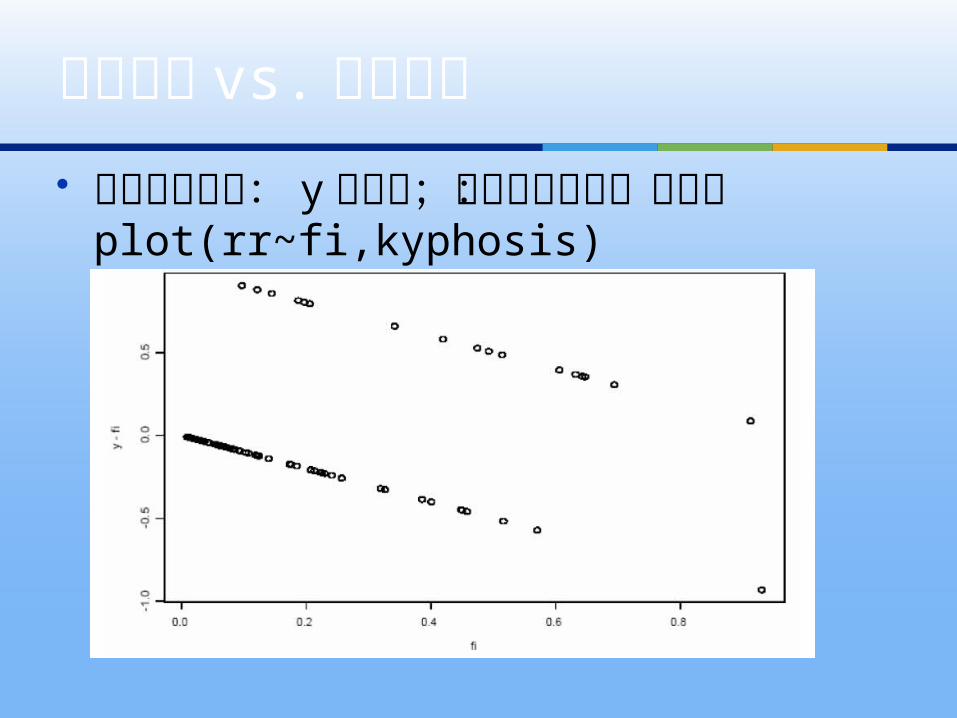
图中横坐标为： y 拟合值；纵坐标分别为：拟合值 plot(rr~fi,kyphosis)

响应残差 vs. 拟合的图

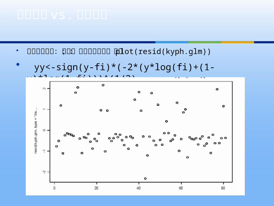
图中横坐标为：序号；纵坐标分别为：残差 plot(resid(kyph.glm)) yy<-sign(y-fi)*(-2*(y*log(fi)+(1-y)*log(1-

fi)))^(1/2)

偏差残差 vs. 序号的图

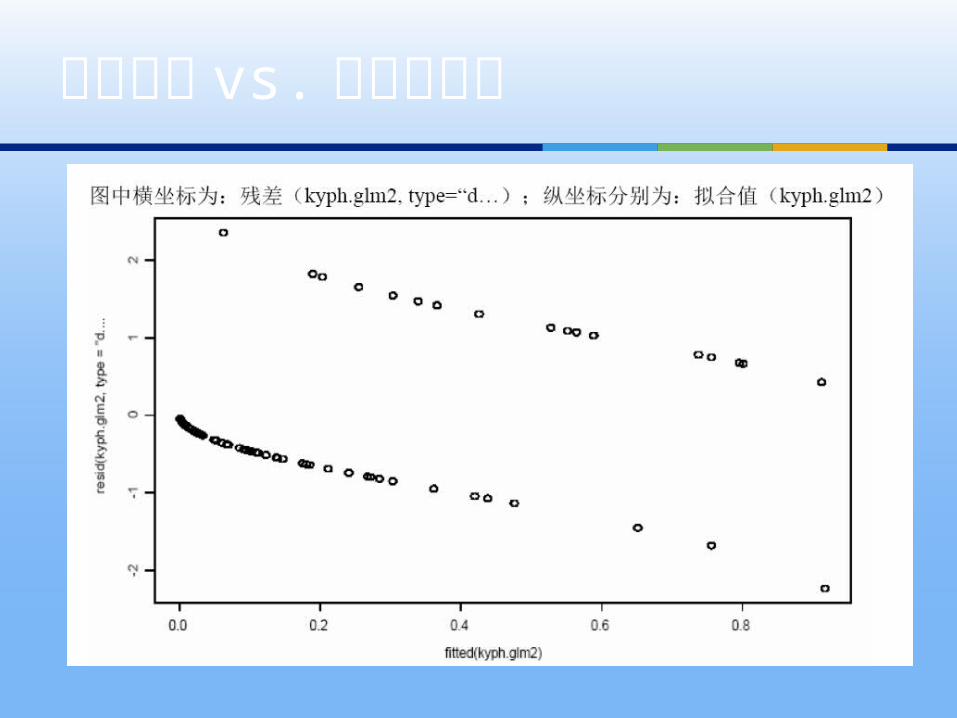
偏差残差 vs. 拟合值的图