M nTHIRTY-THO NODES HMNIMONL ELIDMNT IMI5TINE FUR inOn ULTI-PURPOSE PIOURRN HEM() NYS. POSTUNIMTIE SCHOOL.

U:UL" SSFIE MNTEREY CAR ftKIICEEYOUTH SEP 6 F992 I

s N ICSIIDFS92 UEEEEEEEomhEEEEEEEEEEmhohEEEEI

.355

'-2.0

1111111 .4

1-4 11 P86

3113

NAVAL POSTGRADUATE SCHOOLMonterey, California

DTI

ELECTEJAN2 11987U

THESIS EM

THIRTY-TWO NODES HEXAHEDRONAL ELEMENTSUBROUTINE FOR MULTI-PURPOSE PROGRAM MEF

1 4..by

Anan Sukaneeyouth

September 1986

Thesis Advisor: Gilles Gantin

Approved for public release; distribution is unlimited.

C-,7

or e v

Unclassified* SECURITY CLASSIFICATION OF TI.S PAGE A'. -

REPORT DOCUMENTATION PAGEla REPORT SECURITY CLASSIFICATION lb. RESTRICTIVE MARKINGSUnclassified

2a SECURITY CLASSIFICATION AUTHORITY 3 DISTRIBUTION /AVAILABILITY OF REPORT

2b OECLASSIFICATION /DOWNGRADING SCHEDULE Approved for public release; distributionis unlimited.

4 PERFORMING ORGANIZATION ftf PORT NUMBER(S) S MONITORING ORGANIZATION REPORT NUMBER(S)

15a, NAME OF PERFORMING ORGANIZATION 16b OFFICE SYMBOL 7a. NAME OF MONITORING ORGANIZATIONNaval Postgraduate School (if applicable)

________________________ j 69 Naval Postgraduate School

15C ADDRESS (City. State, and ZIP Code) 7b. ADDRESS (City, State, "n ZIP Code)

*Monterey, CA 93943-5000 Monterey, CA 93943-5000

Ba NAME OF FUNDING /SPONSORING 8b. OFFICE SYMBOL 9. PROCUREMENT INSTRUMENT IDENTIFICATION NUMBERORGANIZATION (if applicable)

8c ADDRE SS (City, State, and ZIP Code) 10 SOURCE OF FUNDING NUMBERSPROGRAM IPROJECT ITASK IWORK UNITELEMENT NO NO NO jACCESSION NO

ITITLE (include Security Classification)THIRTY-TWO NODES HEXAHEDRONAL ELEMENT SUBROUTINE FOR MULTI-PURPOSE PROGRAM MEF

2 PERSONAL AUTHOR(S)Anan Sukaneeyouth, LT, Thailand Navy

Is '3a, TYPE OF REPORT 13b TIME COVERED 14 DATE OF REPORT (Year, Aonth,Oay)1 PAGE QuNTEngineers Thesis FROM TO 1986 September 7

6 SUPPLEMENTARY NOTATION

COSATI CODES IS SUBJECT TERMS (Continue on reverse if necessary "n identify by block number)~ELD GROUP SUB-GROUP -Consistent Load Vector,' Computer Program, Finite Element;

Integration Points; Jacobian Matrix,' Reference Element,

Shape Function.'9 ABSTRACT (Continue on reverie if necessary and identify by block number)

A general finite element program of moderate complexity called MEF is organizedto contain a library of one, two, and three-dimensional elements for the solution ofproblems from a wide variety of diciplines. A cubic, thirty-two node, three dimensional

* isoiparametric element was developed. With such an element very complex structures couldbe solved with a very course mesh.

0 0 'j S'PjjTON, AVAILABILITY OF ABSTRACT 21 ABSTRACT SECURITY CLASSIFICATION

(2 %:CLASSiFIED,1UNLiMITED 0 SAME AS RPT 0 DTIC .SERS Unclassified"2a %'.AE OP RESPONSIBLE .NDIVDUAL 22b~ TELEPHONE (include Area Code) 2c OPI E SM8C

Profso 1ie Cantin 4 8 646-2364 6CDD FORM 1473,.84 MAR 83 APR edition rr'ay be used until exhausted SECURITY CLASSIFCAT,(c% C);

All other editions are obsolete

77- 7 .-- - - ---

Approved for public release; distribution is unlimitcd.

Thirty-Two Nodes Hexahedronal Element Subroutine

for Niulti-Purpose Program NIEF

by

Anan SukanecyouthLieutenant, Royal Thai Navy

B.S., Royal Thai Naval Academy, 1978

Submitted in partial fulfillmcnt of therequirements for the dcgrees of

MASTER OF SCIENCE IN MECHANICAL ENGINEERINGand

MECHANICAL ENGINEER

from the

NAVAL POSTGRADUATE SCIOOLSeptembcr 1986

Author: ~~Icz~y~~Anan Sukaneeyouth

Approved by:_6 4~(lilcs Ca tin "lhesis Advisor

A.J. ealey, Chairman,I)epartmet of lcchanical Enginecring

* / John N. Dyer,* Dean of Science and Engineering

2

.S --. .. -,, Z :;,-.;.;, ;.-;.,"; ;; -- ;- - '-."--- --- '? "" ":"" -'----... o .,, . . ].% .,. € ,€.., ,' ,- . e "%-,-a,."~'r "-."-. -

- -. ,.,.-.,-- . .- ,.-. ,.' ,,, - "-." -." - -U - _-_-

. *- 7.o 7. T.

ABSTRACT

A general finite element program of moderate complexity callcd MEF is

organized to contain a library of one, two, and three-dimensional elements for the

solution of problems from a wide variety of diciplines. A cubic, thirty-two node, three

dimensional isoparametric element was developed. With such an element very complex

structures could be solved with a very course mesh.

Accession For

NTIS GRA&IDTIC TABUnannounced LIJustification

" ByDistribution/

Availability Codes~Avail and/or

Dist Special "

'a.,

,.4

*~~~~~~~~~~- -w- w ~ - -~- - . -- s - --

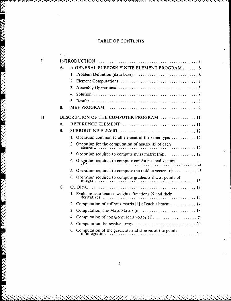
TABLE OF CONTENTS

INTROD UCTION .............................................. 8A. A GENERAL-PURPOSE FINITE ELEMENT PROGRAM ....... 8

1. Problem Definition (data base): ............................ 8

2. Element Computations: ................................... 83. Assem bly Operations: .................................... 8

4. Solution: ............................................... 8

5. R esult: ................................................ 8

B. M EF PROG RA M ......................................... 9

II. DESCRIPTION OF THE COMPUTER PROGRAM ................ 11

A. REFERENCE ELEMENT ................................. 11

B. SUBROUTINE ELEM03 ................................... 12

I. Operation common to all element of the same type: ........... 12

2. Operation for the computation of matrix [k] of eachelem ent: ............................................ 12

3. Operation required to compute mass matrix [m]: ................ 12

4. Operation required to compute consistent load vectors(0 : .................................................12

5. Operation required to compute the residue vecter {r}: .......... 136. Operation required to compute gradients 0 u at points of

in tegral: ... ..... .... ..... .... .... ..... ..... ...... .. .13

C . C O D IN G . ............................................... 1 31. Evaluate coordinates, weights, functions N and their

derivatives .......................................... 132. Computation of stiffncss matrix [k] of each element .......... 14

3. Computation The Mass Matrix [ml ......................... 18

4. Computation of consistent load vector {t ................... 19

5. Computation the residue array . ........................... 2()

6. Computation of the gradients and stresses at the pointsof integration . ....................................... 20

41

4 j q ' . ,, . o , . . , ' ' ' ° . ., ' ° ' ' ' ' "

" , q . - ' - ' ' - ' , ' ' , ' " . ~ " . . * - . , . .

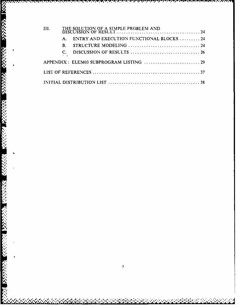
Ill. THE SOLUTION OF A SIMPLE PROBLEM AND

DISCUSSION OF RESULT ..................................... 24

A. ENTRY AND EXECUTION FUNCTIONAL BLOCKS ......... 24

B. STRUCTURE MODELING ................................ 24

r C. DISCUSSION OF RESULTS ............................... 26

APPENDIX: ELEM03 SUBPROGRAM LISTING ......................... 29

LIST OF REFERENCES ................................................ 37

INITIAL DISTRIBUTION LIST ......................................... 38

.JI

.5.L

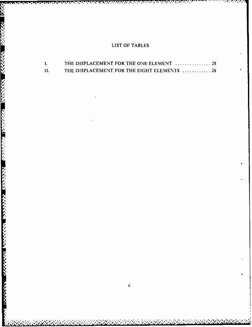
LIST OF TABLES

I. THE DISPLACEMENT FOR THE ONE ELEMENT ............... 28

I. THE DISPLACEMENT FOR THE EIGHT ELEMENTS ............ 28

6

II H IPAEETFRTE IH LMNS.....2

,0

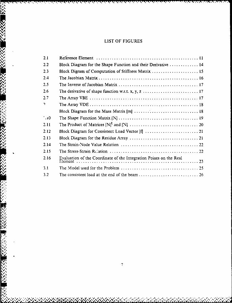
LIST OF FIGURES

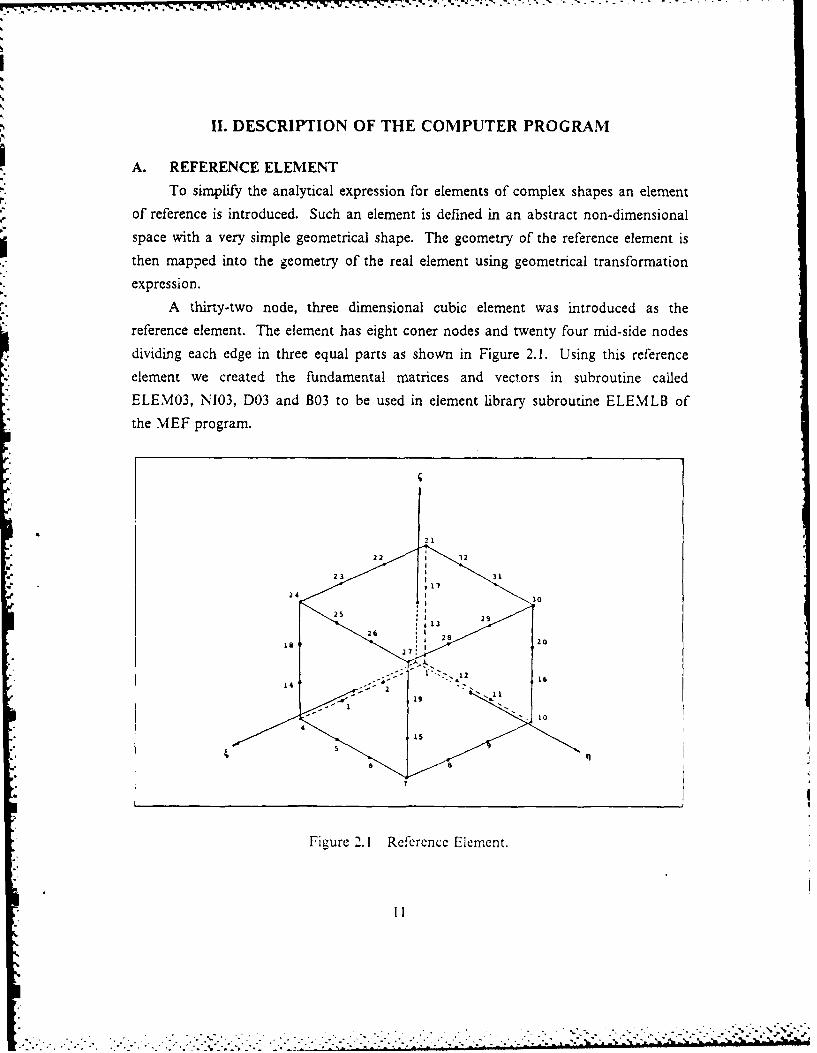
2.1 Reference Elem ent .............................................. I

2.2 Block Diagram for the Shape Function and their Derivative ............. 14

2.3 Block Digram of Computation of Stiffness Matrix ..................... 15

2.4 The Jacobian M atrix ............................................. 16

2.5 The Inverse of Jacobian M atrix .................................... 17

2.6 The derivative of shape function w.r.t. x, y, z ......................... 17

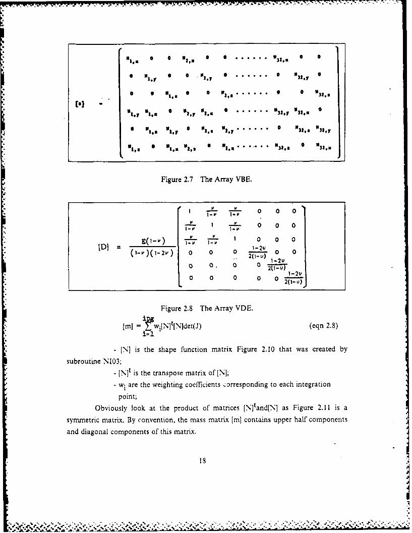
2.7 The A rray VBE ................................................. 17

The A rray V D E ................................................. 18

Block Diagram for the Mass Matrix [ml ............................. 1810 The Shape Function M atrix [NJ .................................... 19

2.11 The Product of M atrices [Nit and [NJ ............................... 20

2.12 Block Diagram for Consistent Load Vector [f]........................ 21

2.13 Block Diagram for the Residue Array ............................... 21

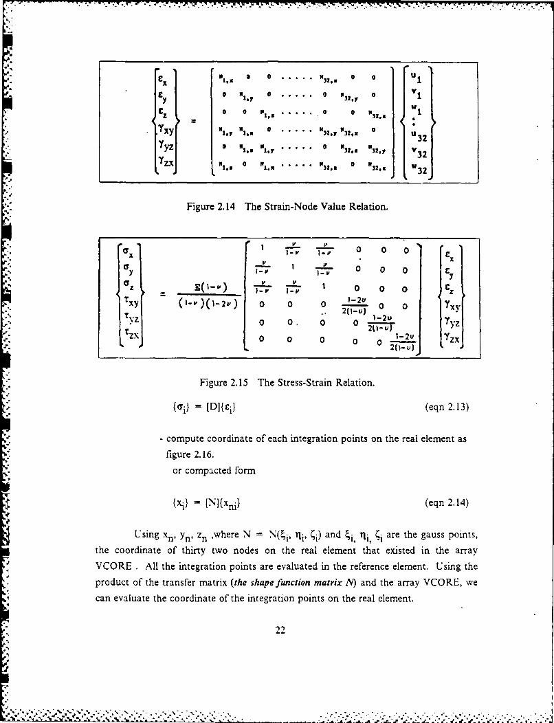
2.14 The Strain-Node Value Relation ................................... 22

2.15 The Stress-Strain Rt'ation ........................................ 22

2.16 Evaluation of the Coordinate of the Integration Points on the RealE lem ent ....................................................... 23

3.1 The M odel used for the Problem ................................... 25

3.2 The consistent load at the end of the beam ........................... 26

II

I 6

I. INTRODUCTION

A. A GENERAL-PURPOSE FINITE ELEMENT PROGRAMA general-purpose finite element program should be able to solve a variety of

problems from the number of disciplines: linear and non-linear, static and dynamicproblem of elasticity, fluid mechanics, heat transfer, etc. and can solve problems oflarge size involving a variety of elements.

A general program is going to be voluminous and complex. It is, however,desirable that:

0 its logic be easily understood;

* one or many of its parts be easily modifiable;* it offers possibilities to tailor its facilities for the solution particular classes of

problems.The program should have a modular structure, with the modules made as

independent from one another as is practicable. The following modular operations arerecognized:

1. Problem Definition (data base):- node coordinates and clement connectivities;

- nodal element properties;

- boundary conditions.2. Element Computations:

- integration points and associated weights;

- interpolation functions and their derivatives;- Jacobian matrix, inverse, and determinant;- element matrices and vectors: [ki, [in], {0, etc.

3. Assembly Operations:- assemblage of master matrices and vectors, IK], [M.I, etc.

4. Solution:- factorization of master matrices and solution of equations.

5. Result:

- output of nodal variables and other calculated quantities: gradients,

reactions, etc.

o'S

.,', ; ', ... ,+.' .. :. -+.-+. .- , .: .'- .. >+ .- . ..- .- , "- ;...: ,. .+. , ._ -... - + .

I -P 0 Y7 - -lj

Subroutines implementing the various operations described above are

contained in all finite element codes. The flow of information between these

operations is problem dependent; linear, non-linear, static, and dynamic problems all

require logic of their own.

B. MEF PROGRAM

A program of medium complexity, called MEF, implementing the techniques of

general-purpose program that can solve a large variety of boundary value problems of

mathematical physics. It is written in FORTRAN IV and can be easily adaptable to

various computers.

The main program 'controls the flow of all information through the functional

blocks by transferring control to a subroutine called BLNNNN when the block calling

card NNNN is encountered in the input file. The subroutine BLNNNN then performs

preliminary functions s-uch as logical unit identification, and reading of control

parameters for the creation of' various files and tables. The subroutine then calls

subroutine EXNNNN. In all cases, subroutine BLNNNN provides appropriate default

parameters which will be overridden by user values if specified. Subroutine EXNNNN

then performs the major operations of the block by calling on the needed subroutines

in the MEF library. The above protocol holds for all blocks except STOP, COMT,

and IMAG. All the functions of COMT and IMAG are performed by subroutine

BLNNNN, and the function of block STOP is performed by the main program.

The executable functional blocks contained in the MEF are:

BLOCK FUNCTION

SOLR Assemblage of distributed load.

LINM Solution of linear problem with global matrix in core.LIND Solution of linear problem with global matrix out of core.

NLIN Solution of stationary non-linear problem.

TIEMP Solution of unsteady problem (linear or non-linear).

VALP Eigenvalues and cigenvectors.

The various blocks designed for execution of the various computations have

similar structures since thcy have to:

0 construct element and load matrices;

* assemble global matrices and vectors;

e factori/e and solve the system of equations:

I°

I)

0 ... . . . .. .N . , • ° , -% % • % - - , , -% '.. - - - . .. "° '. % . .

i'k d.

* output the results.

Using the constructed elements and load matrices, the subroutine element librarv

ELEMLB is called. This library contains subroutines that define the individual element

types. The ELEMO3 subroutine, a thirty-two node, three dimensional isoparametic

element was developed and added to the element library. This new element allowed the

solution of linear elastic structures composed of homogeneous and isotropic materials.

Multiple sample problems were developed to fully exercise use of this new

element. An indepth investigation was then conducted to determine the limit of

computational ability using the newly defined element to represent physical

phenomenons.

N

II(

II. DESCRIPTION OF THE COMPUTER PROGRAM

A. REFERENCE ELEMENT

To simplify the analytical expression for elements of complex shapes an elementof reference is introduced. Such an element is defined in an abstract non-dimensionalspace with a very simple geometrical shape. The geometry of the reference element is

then mapped into the geometry of the real element using geometrical transformation

expression.

A thirty-two node, three dimensional cubic element was introduced as thereference element. The element has eight coner nodes and twenty four mid-side nodesdividing each edge in three equal parts as shown in Figure 2.1. Using this reference

element we created the fundamental matrices and vectors in subroutine calledELEM03, N103, D03 and B03 to be used in element library subroutine ELEMLB of

the MEF program.

22 1

Fir"22 3 31.,17

24 30

II

26..

2 19 7

12o

y 14

It.9

10 ,,- - . .. -.. .- .'. ., 2 .:...-' " : " -.' .' " - - " ". . i- .- " . i " 2: i- ' -.' -' i . -- " -." - " " * " " " -' -" ," -" -" ",4

-' .' -' --. '. .-. . - . . - ", -"-. -'_ "Z - = " , " - ".. .. .. .., , ,z , . , . ~ r a l~ . ,_L. . , ,_15,

.61 TV TV -3~ -N

B. SUBROUTINE ELEM03

Multi-purpose program MEF is organized to contain a library of one, two, and

three-dimensional elements for the solution of problems from a wide variety of

disciplines. Problems from the mechanics of solids and fluids, heat transfer, etc. have

been solved. For each element type nn, subroutine ELEMnn controls the computation

of all matrices and vectors.

In element type 03, subroutine ELEM03 is organized to create the fundamentalmatrices and vectors that must be numerically integrated using methods of NumericalIntegration described in and the computations ;an be carried out by the following

steps.

1. Operation common to all element of the same type:

- compute the weight wr and the coordinate of integration points;

- construct the functions N (interpolation functions), the tunction 5.'(geometrical interpolation functions) and their derivatives

with respect to 4, %1, 4 at the points of integration.

2. Operation for the computation of matrix [k] of each element:

- initialize the matrix [k];

-for each point of integration r:

9 construct the Jacobian matrix [J] from the derivatives with respect

to ,, , of function N and the nodal coordinates of the element;

* construct the inverse of [J] and its determinant;

* construct the derivatives of functions N with respect to x, y, z

starting from the derivatives with respect of 4, q, ;

* construct the matrices [B and [D];

* accumulate into [k] the values of [Bjt[DI[Bldet(J)wr calculated for

each integration point.

3. Operation required to compute mass matrix [m]:

- initialize [m]

- for each integration point 4r:

" compute Jacobian matrix and its determinant;

• accumulate the values of {N} < N > det(J)wr into matrix [m].

4. Operation required to compute consistent load vectors {f}:

- initialize {f;- for each integration point 4r

? compute the Jacobian matrix and its determinant;

12-p

• ' -" " " r-" ' . . . . .". . ." ""p '" " " '" " " ' ' " " ' " " "

Y P7 -7 7 F- -jf lp -.- V --

* accumulate the values of {N}f v det(J)wr into {f}.5. Operation required to compute the residue vecter (r):

- using the value of {f} from 4;

- for each integration point fr:

* compute matrices [B], 1D, [J] as in 2 above;

* accumulate the product: {f - [Bjt[D][B]{un} wrdet(J) into {r}.

6. Operation required to compute gradients du at points of integral:

for each integration point r :* construct matrix [B] as in 2 above;

* compute and print gradient {4u} = [B]{un}.

The subroutine ELEM03 executes one operation at a time depending on the

value of ICODE. Control variable ICODE specifies which element operation is

desired, and expression of this variable as follows:

ICODE = I initialization of the characteristic parameters of an element

(number of nodes, number of degrees of liberty).

ICODE = 2 operations required by a given referance element which are

independent of the real geometry; construction ofinterpolation function N and their derivative with

respect to 4 at the points of integration.

ICODE = 3 construction of matrix jkl in array VKE.

ICODE = 4 construction of tangent matrix needed for non-linear

problems in array VKE.

ICODE = 5 construction of mass matrix [mi] in array VKE.

ICODE = 6 computation of residual vector {r} in array VFE.

ICODE = 7 computation load vector {f) in array VFE.

ICODE = 8 computation and printing of gradients {u}.

C. CODING.

I. Evaluate coordinates, weights, functions N and their derivatives

Integration formular for numerical integration is the following form.

I = wly( ) (eqn 2.1)

where

6 ,1 are the coordinates of integration point T in , q, system

coordinate corresponding to weight w;

13

P"

_ . .

f . LI4.wv :,

- wI are the weights corresponding to integration point number;- IPG are the total number of integration points.

A choice of 2, 3 or 4 integration points by dimension can be made in

subroutine GAUSS [Ref. l:p. 265], giving respectively 8, 27 and 64 integration points,

the weights corresponding to the integration points and their coordinates. They are in

the array called IPG, VCPG and VKPG respectively.

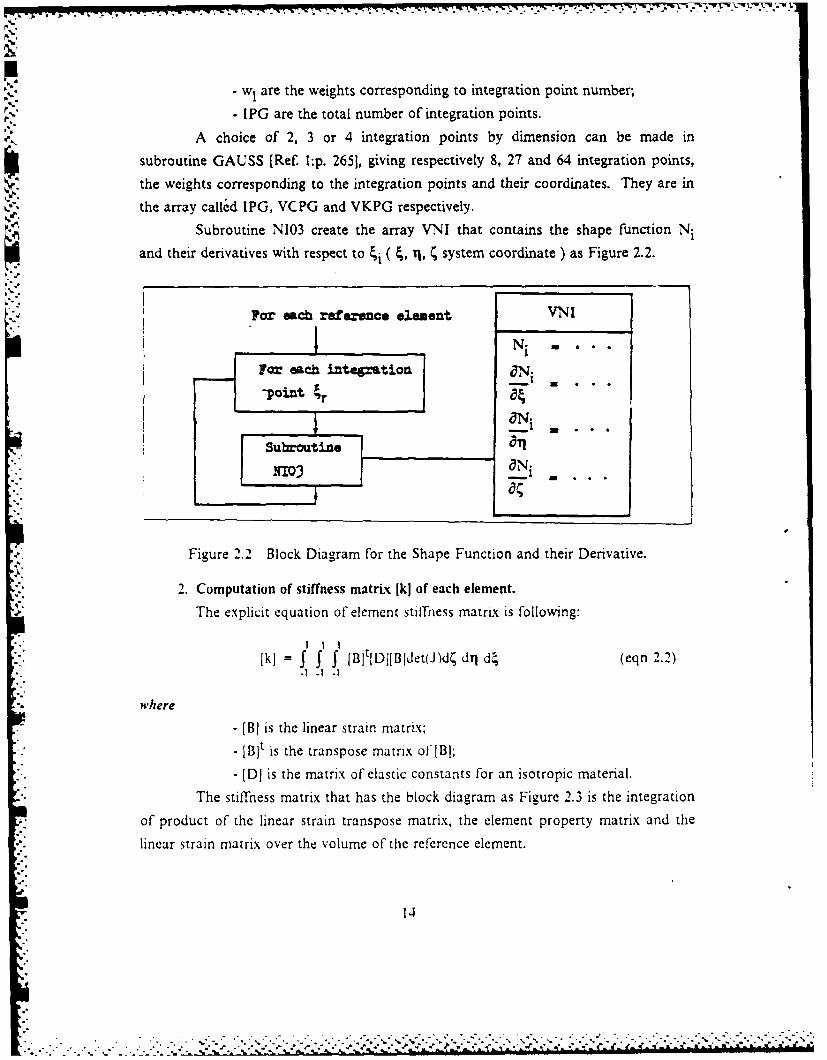
Subroutine N103 create the array VNI that contains the shape function Ni

and their derivatives with respect to Tu ( ' i' system coordinate ) as Figure 2.2.

........

Po each reference element VNI~Ni'

Fo= each integz tion ON-

-pointtr a4

- 0_.Ni

a;

Figure 2.2 Block Diagram for the Shape Function and their Derivative.

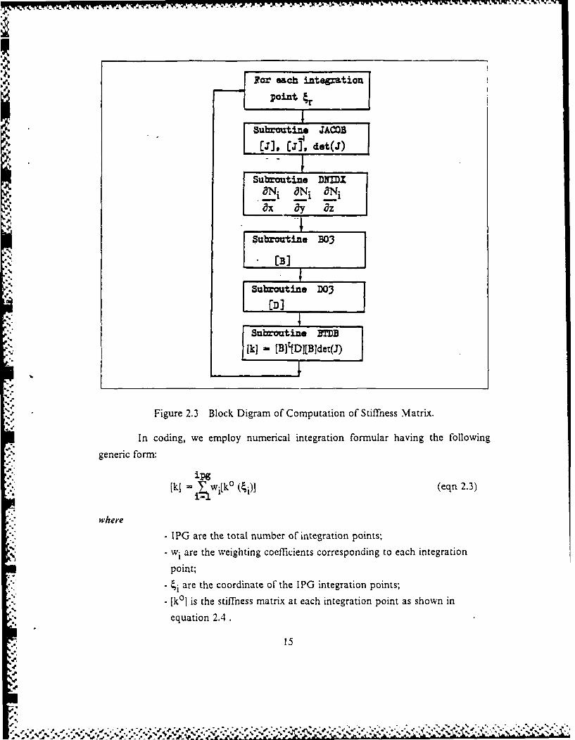
2. Computation of stiffness matrix [k] of each element.

The explicit equation of element stiffness matrix is following:

[k] = 5 5" [BIt[DI[BIdet(JMd; dq d4 (eqn 2.2-. -1 -1 -1

where

- [B] is the linear strain matrix-

- [Bit is the transpose matrix of [BI

- [D] is the matrix of elastic constants for an isotropic material.The stiffness matrix that has the block diagram as Figure 2.3 is the integration

of product of the linear strain transpose matrix, the element property matrix and the

linear strain matrix over the volume of the reference element.

.. 14

For each integation

Point

Suboutine JACOB

["j, (J], det(J)

Subroutine DIZ

'i's

Subroutine D3

[k] - [B]tfD][Bjdet(J)

Figure 2.3 Block Digram of Computation of Stiffness Matrix.

In coding, we employ numerical integration formular having the following

generic form:

ipg-~w~°]Wi~k (4i)] (eqn 2.3)

where

- IPG are the total number of integration points;

- wi are the weighting coefficients corresponding to each integration

point;

" are the coordinate of the IPG integration points;

- [k0l is the stiffness matrix at each integration point as shown inequation 2.4.

15

-S

t5

P.. W 7-7- _ ro ., .. L " .. , *., . J L•

-'

- : -"-- _ .. . w-. * - . . .. • . _ . . ._.. .- • •~*

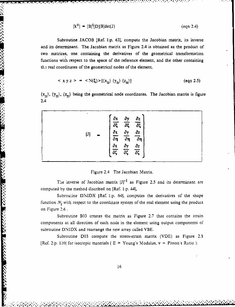
[k° ] = [B]t[DI[Bldet(J) (eqn 2.4)

Subroutine JACOB [Ref. 1:p. 63], compute the Jacobian matrix, its inverse

and its determinant. The Jacobian matrix as Figure 2.4 is obtained as the product of

two matrices, one containing the derivatives of the geometrical transformation

functions with respect to the space of the reference element, and the other containing

th- real coordinates of the geometrical nodes of the element.

< x y z > < N(4)> [{Xn} {yn {Zn}] (eqn 2.5)

{Xn), {Yn}, {Zn} being the geometrical node coordinates. The Jacobian matrix is figure

2.4

0x ' az

ax ay az

ax By az

L4 a;

Figure 2.4 The Jacobian Matrix.

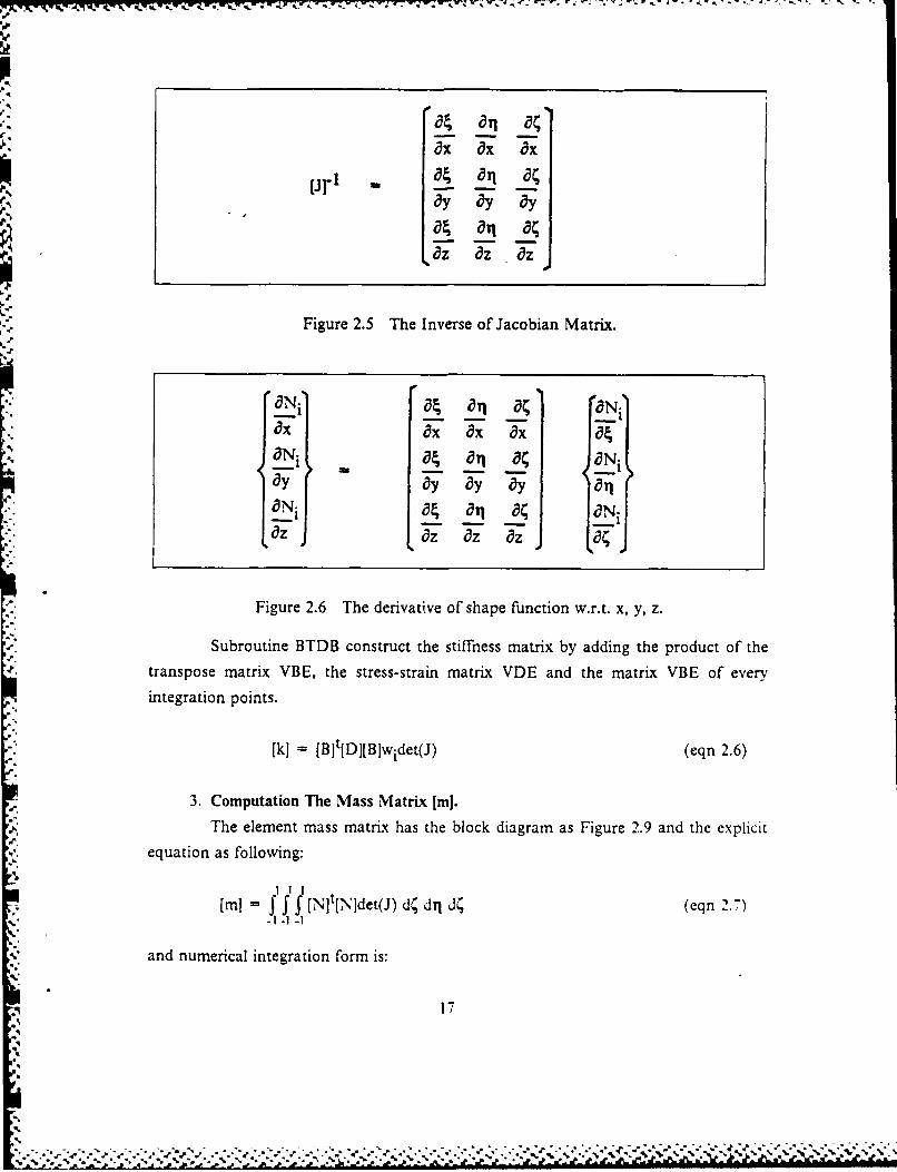
The inverse of Jacobian matrix [J]- 1 as Figure 2.5 and its determinant are

computed by the method discribed on [Ref. l:p. 44],

Subrou:ine DNIDX [Ref. l:p. 64], computes the derivatives of the shape

function Ni with respect to the coordinate system of the real element using the product

on Figure 2.6.

Subroutine B03 creates the matrix as Figure 2.7 that contains the strain

components at all direction of each node in the element using output components of

subroutine DNIDX and rearrange the new array called VBE.

Subroutine D03 compute the stress-strain matrix (VDE) as Figure 2.8

[Ref. 2:p. 1101 for isotropic materials ( E = Young's Modulus, v - Pisson's Ratio ).

16

%PP.

"a - ° . , - ,

ax 8x 8x

ay y y

az 8z az

Figure 2.5 The Inverse of Jacobian Matrix.

.11

5_i.O 8j __ 8Ni

ayy 8y y

az Oz 8Z TZ

Figure 2.6 The derivative of shape function w.r.t. x, y, z.

4. Subroutine BTDB construct the stiffness matrix by adding the product of thetranspose matrix VBE, the stress-strain matrix VDE and the matrix VBE of every

integration points.

[k] - [Blt[DI[Blwidet(J) (eqn 2.6)

3. Computation The Mass Matrix [ml.The element mass matrix has the block diagram as Figure 2.9 and the explicit

equation as following:

[m] =f J[N]t[Nldet(J) d; dq d; (eqn 2.7)-1-1

and numerical integration form is:

17

I q '. -.-, .: .> : , : .: .: , .: . - .: , : .-: , : ..2 ..... : - .; ..-: ' o , ...- -, : .: : .-, : - -, ., -; i , -,- , - : S :

n Io, 0 0 . o . N32,X a 0

O H 0 a6 . y o 0 0 . . 32' •

O 6 Nla O * Ill. . . ... 0 0 N 32.2

or 1 o .32 .3 22 0

I.. I0 , 0 0 Its N 01n N"1o

1*8e a IIIon 0go O0 0~ n Ple 0 a • 29 • 9 13t O 32,x

Figure 2.7 The Array VBE.

I , , 0 0 0

1 - 0 0 0t - 1-u.

0 0 0 0 0 0.1I 20-0 1-2

E(1-"') I-L, 1-,, 1 aO1 = 1- 2u

(1-)(1-2) o 0 o 2- ) o

01-2u 21-2u)

Figure 2.8 The Array VDE.

[m] = i[Nlt[Nldet(J) (eqn 2.8)1.=1

[NI is the shape function matrix Figure 2.10 that was created bysubroutine N103;

- [N]t is the transpose matrix of [N];

- wi are the weighting coefficients corresponding to each integration

point;

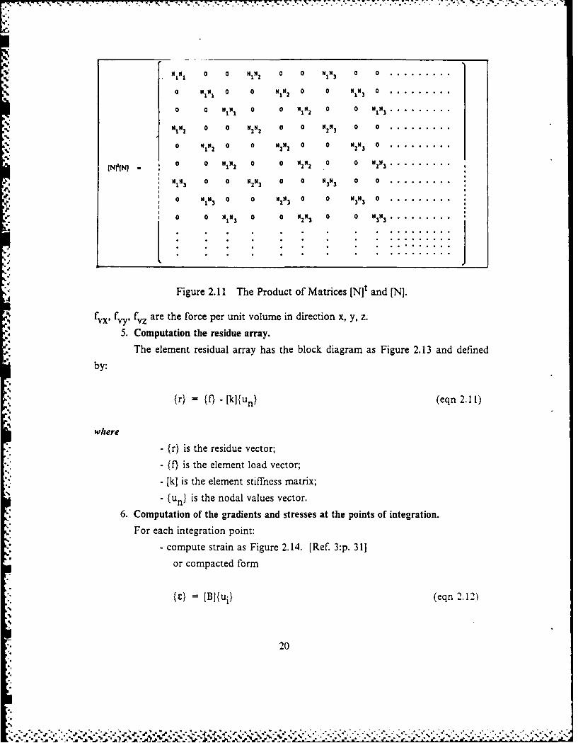
Obviously look at the product of matrices [N]tand[Nl as Figure 2.11 is a

symmetric matrix. By convention, the mass matrix (ml contains upper half components

and diagonal components of this matrix.

18

.. . .A -,".

* -. .. .

For each integration1point ~

N'~~ . u ui JACOB,

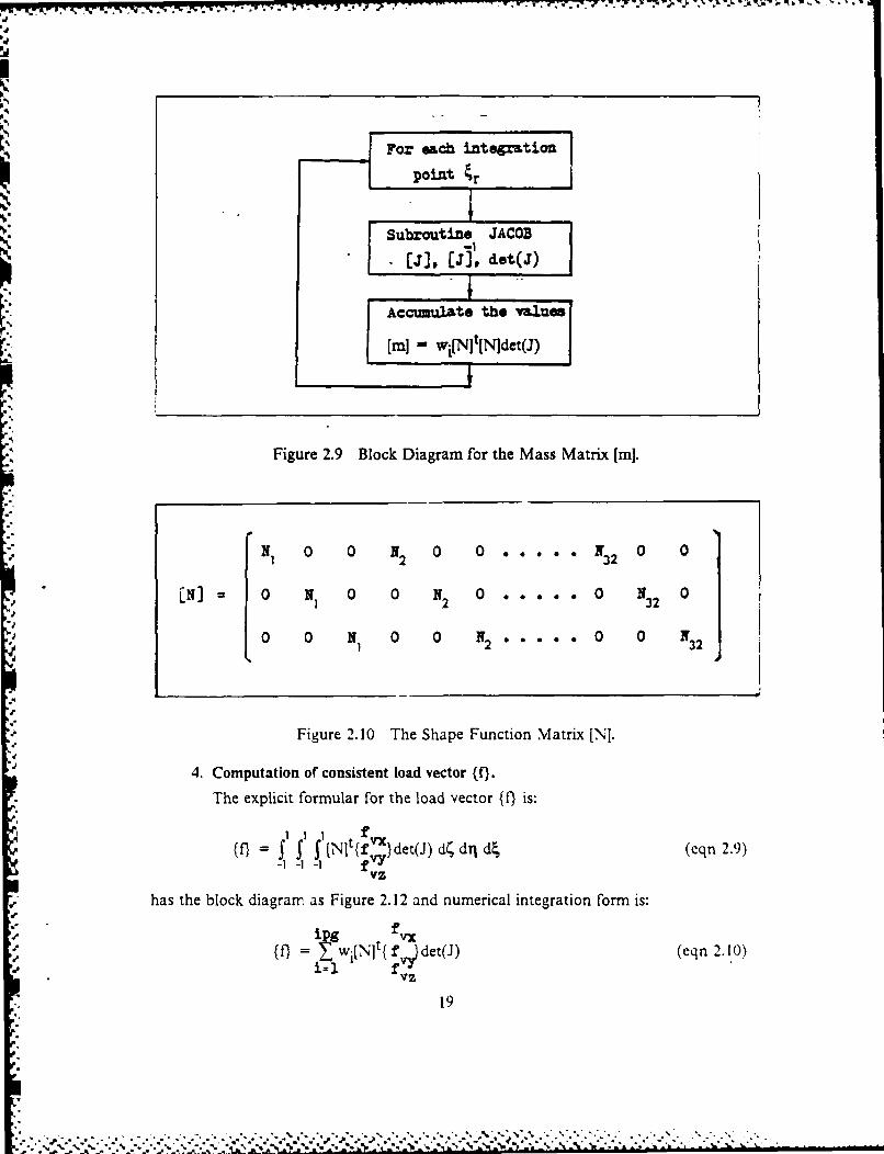
Figure 2.9 Block Diagram for the Mass Matrix [in].

N, 0 0 N2 0 .. . 0 01 2 0 X32

LN)= 0 N1 0 0 N 2 0 .. . 0 N3 0

0 0 N, 0 0 N 2 . . 0 0 N1 N2. . . .0 0 32

Figure 2. 10 The Shape Function Matrix [N].

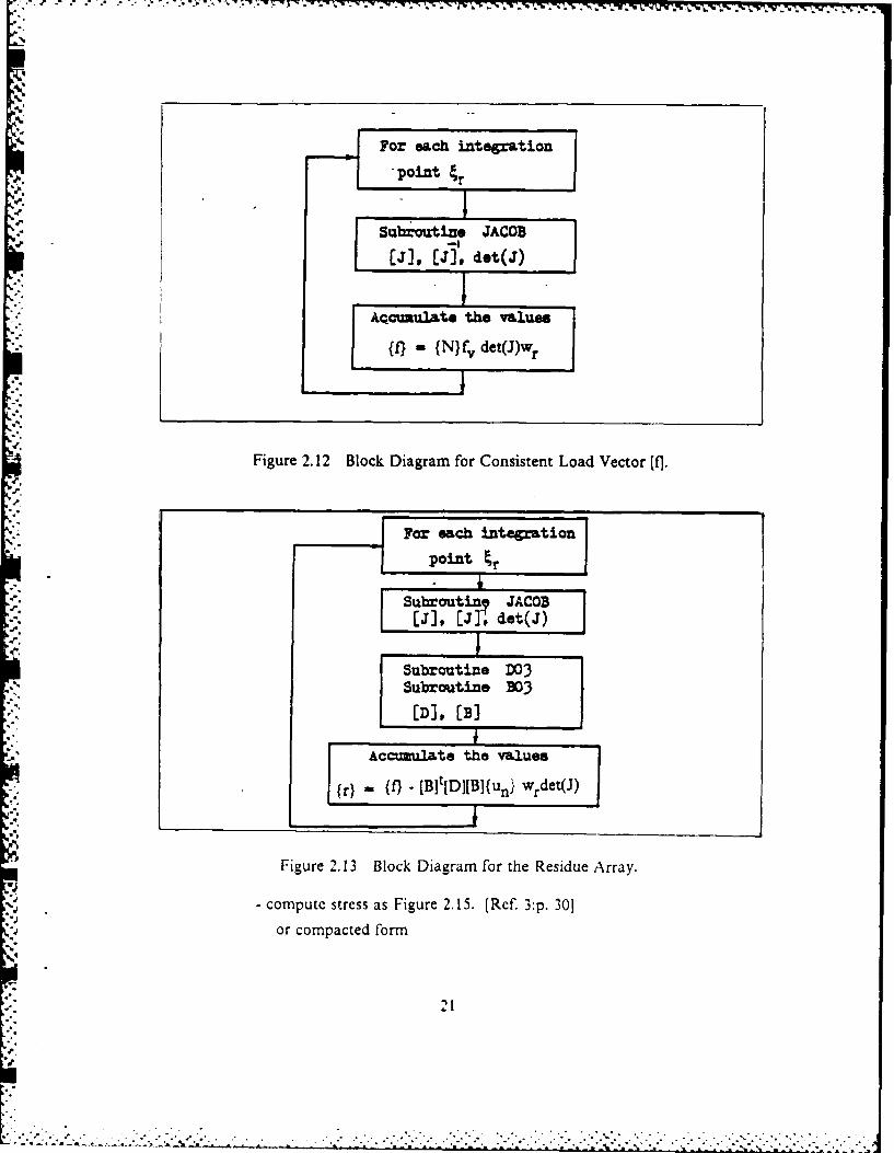
4. Computation of' consistent load vector (f}.

The explicit formular for the load vector {}is:

1 f(I S I ~ [Nit~f }det(J) d; drq d4 (eqn 2.9)

-1 --1 fVYVz

has the block diagranm as Figure 2.12 and numerical integration form is:

(0 = fIt~}det(J) (eqn 2.10)

19

* NN 0 0 NI1N2 0 0 NI N3 0 0 .........

0 MN 0 0 N I W 0 0 IN3 0 . ....... .

0 0 N1N ! 0 0 N 1iN2 0 0 N1 N 3 . . . . . . . . . . . .

"A12 0 0 12N2 0 0 N 3 0 0 .........

0 Mi 0 0 1121N2 0 0 H12113 0 .........

(NIINI 0 0 MIN2 0 0 2H2 0 0 N2"3 .........

1 1 H3 0 0 23 0 0 33 0 . . . . . . . . .

0 NI 3 0 2 0 0 N 3H3 0 ..1..1.. . ..

1 s3 0 Ma~s 0 0 1111 .. ...

I .. . . . ••0. . . . . . . .

Figure 2.11 The Product of Matrices [Nit and [N].

f fy fv are the force per unit volume in direction x, y, z.

5. Computation the residue array.

The element residual array has the block diagram as Figure 2.13 and defined

by:

{r} = {f} -[k]{un} (eqn 2.11)4n)

where

- {r} is the residue vector;

- {f} is the element load vector;

- [k] is the element stiffness matrix;

- fun) is the nodal values vector.

6. Computation of the gradients and stresses at the points of integration.

For each integration point:

- compute strain as Figure 2.14. [Ref. 3:p. 31]

or compacted form

{c} - [B]{ui} (eqn 2.12)

20

wz. : " " " .. : .:*-*,*. .'. ..-' -S-"*"" " ,- -... . -- -.... .. .... :,., , .., , .',,' .',. . ",,..',.. . .. . -: ,. . . ... ,.,. .* .*%. .

- 4 4 -- oin -. - - - - 4

(J), [J], dot(J

Figure 2.12 Block Diagram for Consistent Load Vector [J

For each integrationPoint ~

Subroutin_9 JACOB[J] r J-pdtJ

Subroutine D03Subroutine 303

[D], [BJ

AccuMUlate the values

r} (f) - [BI[D]IB](unj} wrdet(J)

Figure 2. 13 Block Diagram for the Residue Array.

-compute stress as Figure 2.15. [Ref. 3:p. 301or compacted form

N_ V , W :t l. 7 -!

X PI' z a 0 . . . . . 13.x

y 0 Niy 0 . . . . . 0 32 ,V 0 VI

WC 0 0 P1.,. ..... 0 0 N

z 32,z

Y'Yxy N 1 ,, N1 .2 0 ...... N 3 2.y N3 2 ,x 0 U

TyZ 0 .i 1 *........ 32 .s N32 'r"32

T zx 1 ,3 1e~t ..... N 0 3 N3' v3

N f II. 0 N l. .... . 32z 0 32, W32

Figure 2.14 The Strain-Node Value Relation.

0' 0Crx 7' 1.. 0 0 C)

0I-v 0 0 C

(z (I-1) 12 C_ _ 2(_ 0 0 o Yxy

tl 1-2vZ~XJ o o . o o 1,-2u Yz,' 0 0 0 T7Y

Figure 2.15 The Stress-Strain Relation.

{(Ti} = [D]{ci} (eqn 2.13)

- compute coordinate of each integration points on the real element as

figure 2.16.

or compacted form

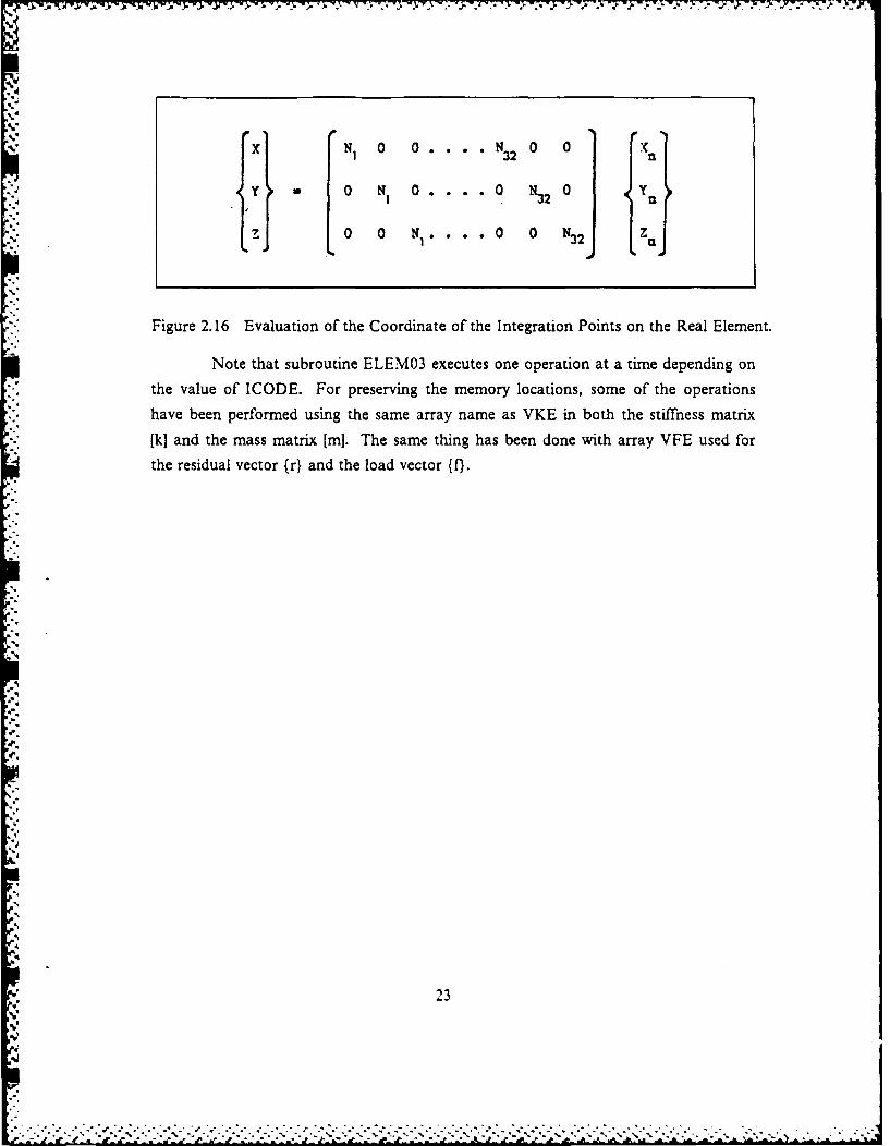
{xi} = [N]{xni} (eqn 2.14)

Using xn , Yn, Zn ,where N = N( i, Qi) and 4i, ii, T i are the gauss points,

the coordinate of thirty two nodes on the real element that existed in the arrayVCORE. All the integration points are evaluated in the reference element. Using the

product of the transfer matrix (the shape function matrix A) and the array VCORE, wecan evaluate the coordinate of the integration points on the real element.

22

" . % " ' , ." % 1 " % . - % % ' . • . . - . . . . . - . - . . . .. ..

rVYW x N, o o .... ~ a aXN1 0 0....N32 0 0X

-*Y - 0 N 0 .... 0 0 Y132

L 0 0 N .... 0 0 N32 Z

Figure 2.16 Evaluation of the Coordinate of the Integration Points on the Real Element.

Note that subroutine ELEM03 executes one operation at a time depending on

the value of ICODE. For preserving the memory locations, some of the operations

have been performed using the same array name as VKE in both the stiffness matrix

[k] and the mass matrix [mi. The same thing has been done with array VFE used for

the residual vector {r} and the load vector {f}.

23

-'...

III. THE SOLUTION OF A SIMPLE PROBLEM AND DISCUSSION OFRESULT

In this.chapter the preparation of input data for the computer program are

described. A simple problem was developed and the investigation was conducted to

determine the ability of this cubic element.

A. ENTRY AND EXECUTION FUNCTIONAL BLOCKS

MEF has specialized functional blocks for the entry, verification and

organization of the data required to define a problem. Block COOR reads the nodalcoordinates and the number of degrees of freedom of each node, it also provides

automatic node generation. Block COND reads the boundary condition. Block PREL

reads element properties if required for element type being used. Block SOLC reads

the concentrated loads. Block ELEM reads the element connectivities; it also reads

element group information when more than one element type is used, if elements have

different properties. This block provides automatic element generation.Other function blocks of MEF for the execution of particular finite element

computations use the data base constructed by entry blocks and augment it by their

results. Block LINM assembles and solves a linear system of equations residing

in-core. Block LIND is similar to the block LINM but the system of equations residesout-of-core in a mass storage device. And block STOP terminates execution of the

problem.

MEF provides various levels of output. The quantity of output desired from agiven block is controlled by a parameter on the block calling card, described in detial

[Ref l:pp. 440)-447j, which ranges from 0 (the assumed value) to 4. The default value

provides all the information needed to verify the input stream and obtain the desired

answers while the value I thru 4 provid? various level of verbosity.

B. STRUCTURE MODELINGThe first step in applying a Finite element solution to the problem is the selection

of an appropriate mesh. In many case an extrapolation of the results will be required

and hence more than one mesh will have to be selected. The mesh size solution does

not follow any oredetermined rules and will. in general, depend on the nature of the

problem and the judgement of the analyst. .\n abitrary numbering convention is

2-4

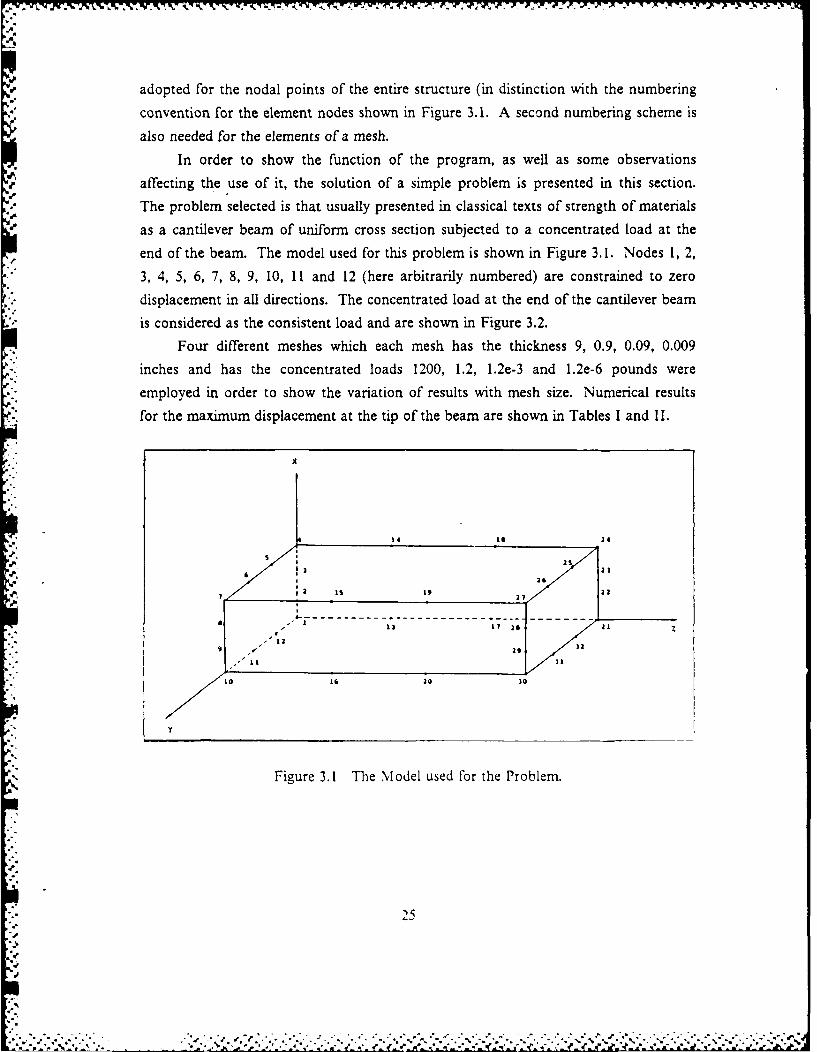
adopted for the nodal points of the entire structure (in distinction with the numbering

* convention for the element nodes shown in Figure 3.1. A second numbering scheme is

also needed for the elements of a mesh.

In order to show the function of the program, as well as some observations

affecting the use of it, the solution of a simple problem is presented in this section.

The problem selected is that usually presented in classical texts of strength of materials

as a cantilever beam of uniform cross section subjected to a concentrated load at the

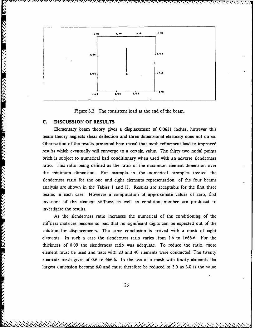
end of the beam. The model used for this problem is shown in Figure 3.1. Nodes 1, 2,

3, 4, 5, 6, 7, 8, 9, 10, 11 and 12 (here arbitrarily numbered) are constrained to zero

displacement in all directions. The concentrated load at the end of the cantilever beam

is considered as the consistent load and are shown in Figure 3.2.

Four different meshes which each mesh has the thickness 9, 0.9, 0.09, 0.009

inches and has the concentrated loads 1200, 1.2, 1.2e-3 and 1.2e-6 pounds were

employed in order to show the variation of results with mesh size. Numerical results

for the maximum displacement at the tip of the beam are shown in Tables I and I I.

X

525

.6 **

ar """ 1317 20'1

lO G 0 30

Figure 3.1 The .Model used for the Problem.

/ 3/1 3/1 -/10

3/16/ 3/10

p 1/6 3/10 3/1

Figure 3.2 The consistent load at the end of the beam.

C. DISCUSSION OF RESULTS

Elementary beam theory gives a displacement of 0.0631 inches, however this

beam theory neglects shear deflection and three dimensional elasticity does not do so.

Observation of the results presented here reveal that mesh refinement lead to improved

results which eventually will converge to a certain value. The thirty two nodal points

brick is subject to numerical bad conditionary when used with an adverse slenderness

ratio. This ratio being defined as the ratio of the maximum element dimension over

the minimum dimension. For example in the numerical examples treated the

slenderness ratio for the one and eight elements representation of the four beamsanalysis are shown in the Tables I and I. Results are acceptable for the first three

beams in each case. However a computation of approximate values of zero, first

invariant of the element stiffness as well as condition number are produced to

investigate the results.

As the slenderness ratio increases the numerical of the conditioning of the

stiffness matrices become so bad that no significant digits can be expected out of the

solution for displacements. The same conclusion is arrived with a mesh of eight

elements. In such a case the slenderness ratio varies from 1.6 to 1666.6. For the

thickness of 0.09 the slenderness ratio was adequate. To reduce the ratio, more

element must be used and tests with 20 and 40 elements were conducted. The twenty

elements mesh gives of 0.6 to 666.6. In the use of a mesh with fourty elements the

largest dimension become 6.0 and must therefore be reduced to 3.0 as 3.0 is the value

26

" " " , " " " " ""- " _ ' . ... " " " " " \- . ... .

of 120/40. Runs with such a mesh were then performed to confirm our results. On the

basis of all these runs and the value of the condition number of these matrices it seems

that a slenderness ratio of approximately 150 could still be used to give results with 6

significant digits in the answers, however further examples must be treated before a

conclusion could be reached.

These are observations essentially made on the results of a simple problem. Thus

no firm rules regarding the use of the newly element can be established and further

experimention with different problems has to be conducted for this purpose.

,o. 27

,ell

i •

i4

.TABLE I

THE DISPLACEMENT FOR THE ONE ELEMENT

S lndernessThickness Ratio Zero a tj ).mal Irin Number Displacemt

9 13.3 0.24o-5 -0.54.-5 7.27ll 3.72o10 3.14e+4 1.18.06 -0.0581

0.9 133.3 0.76e-5 -0.16e-4 7.11e12 1.64.ll 7.42e+1 2.22.09 -0.0515

0.09 1333.3 0.74e-4 0.16.-2 7.11.13 1.64*12 7.420-2 2.22.13 -0.0486

* 0.009 13333.3 0.74e-3 0.56s-6 7.11s14 1.64.13 7.42e-3 4.59e15

TABLE II

THE DISPLACEMENT FOR THE EIGHT ELEMENTS

Slenderness Z Conditioa

Thickness Ratio Zero Nu £ i &in mber DispLacement

9 1.66 O.33*-6 0.23e-S 3.21.10 4.66.09 1.86.06 2.54.03 -0.0625

0.9 16.6 0.94e-6 0.12e-4 9.12.10 2.06.10 1.60.04 1.29.06 -0.0614

0.09 166.6 0.93e-5 0.97e-4 8.89.11 2.06e11 1.65.01 1.29.10 -0.0597

0.009 1666.6 0.93@-4 0.17e-2 8.88.12 2.06.12 1.36*-2 1.32.14

-Irk

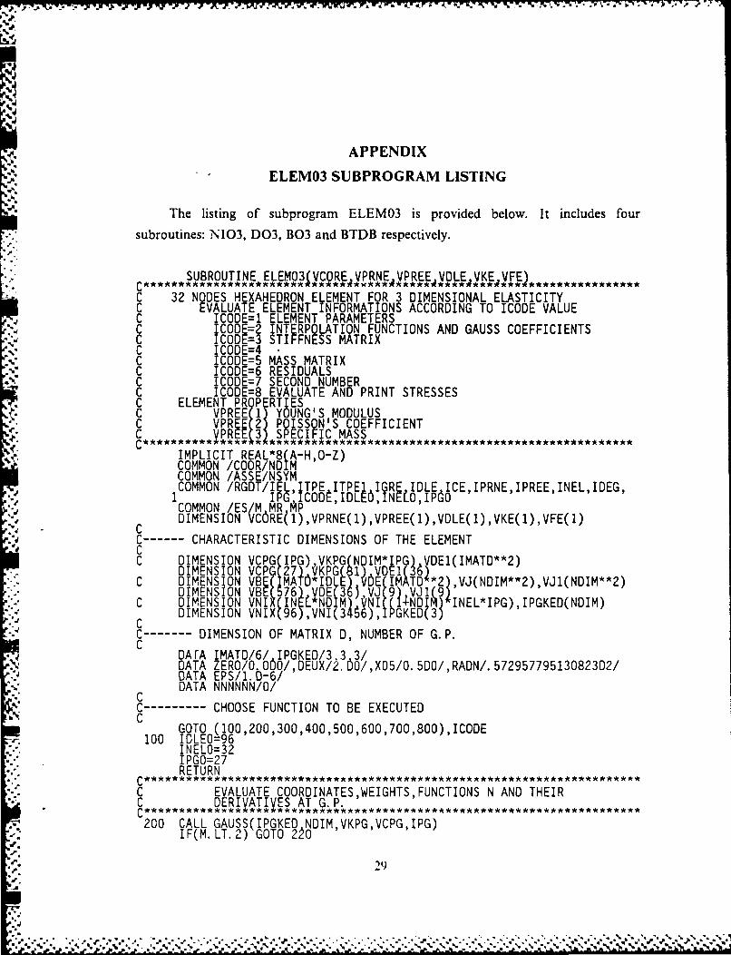
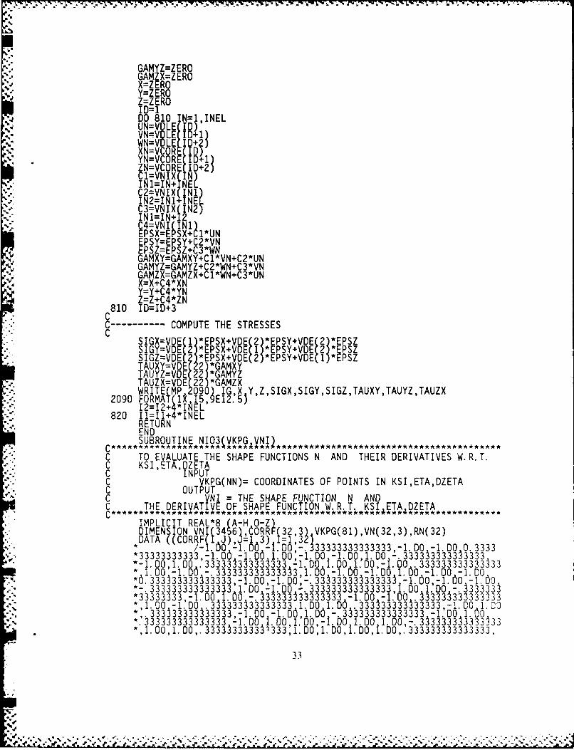
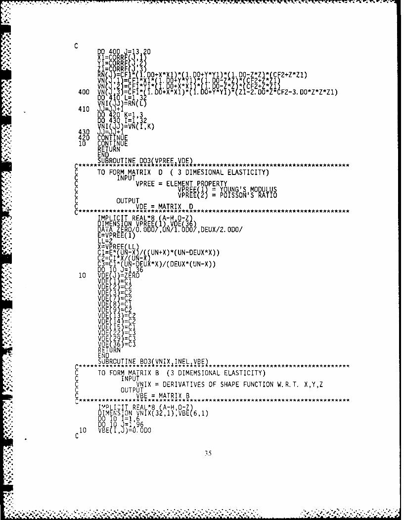
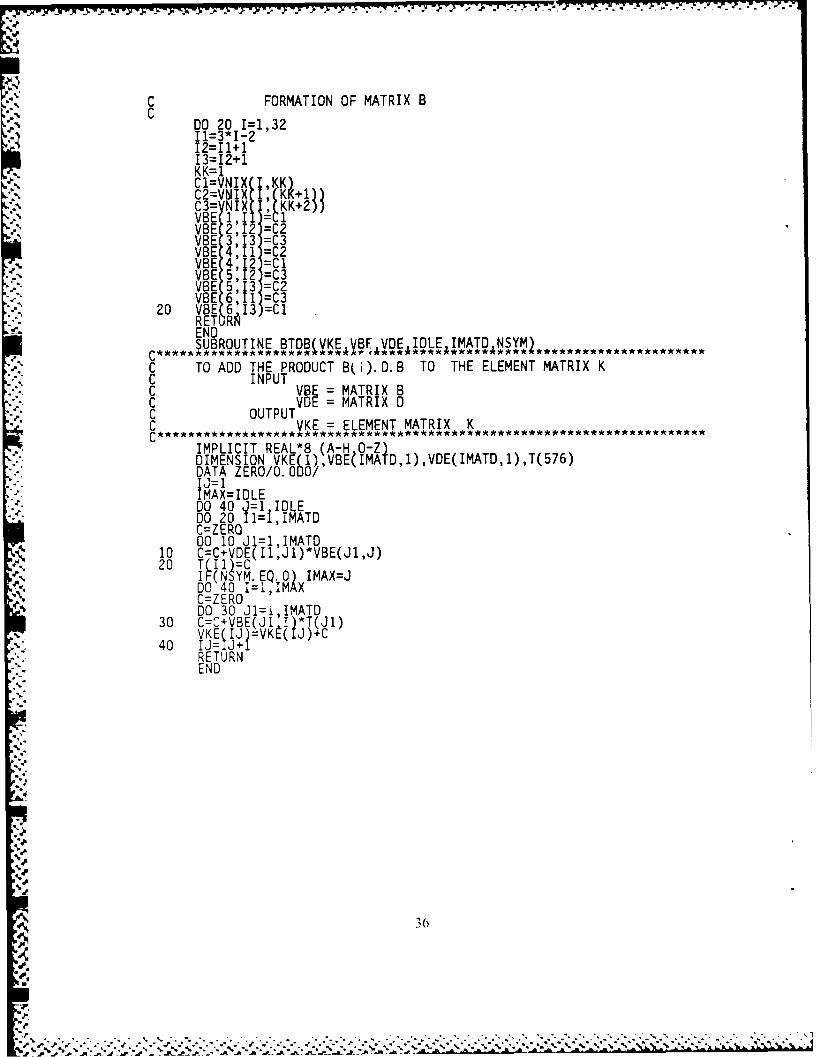
APPENDIXELEM03 SUBPROGRAM LISTING

The listing of subprogram ELEM03 is provided below. It includes four

subroutines: N103, D03, B03 and BTDB respectively.

SUBROUTINE ELEMO3(VCORE.VPRNE.VPREE VDLE VKE VFE)

C 32 NODES HEXAHEDRON ELEMENT FOR 3 DIMENSIONAL ELASTICITYC EVALUATE ELEMENT INFORMATIONS ACCORDING TO ICODE VALUEC ICODE=1 ELEMENT PARAMETERSC ICODE=2 INTERPOLATION FUNCTIONS AND GAUSS COEFFICIENTSC ICODE=3 STIFFNESS MATRIXC ICODE=4C ICODE=5 MASS MATRIXC ICODE=6 RESIDUALSC ICODE=7 SECOND NUMBERC ICODE=8 EVALUATE AND PRINT STRESSESC ELEMENT PR PERTIESC VPREE(1) YOUNG'S MODULUSC VPREE 2) POISSON'S COEFFICIENTC VPREE SPECIFIC MASS

IMPLICIT REAL*8(A-H,O-Z)COMMON /COOR/NDIMCOMMON /ASSE/NSYMCOMMON /RGDT/IELITPE ITPE1 IGRE IDLE ICE,IPRNE,IPREE,INEL,IDEG,1 IPGICODE,IDLEO,INEEO,IPGOCOMMON /ES/M MR MPDIMENSION VCORE(1),VPRNE(1),VPREE(1),VDLE(1),VKE(1),VFE(1)C

C ------ CHARACTERISTIC DIMENSIONS OF THE ELEMENTCC DIMENSION VCPG(IPG),VKPG(NDIM*IPGj VDEI(IMATD**2)

DIMENSION VCP G27 VKPG 81).VDE16C DIMENSION VBE(IMAT* IDLE) VE(IMATD *2) VJ(NDIM**2),VJ1(NDIM**2)DIMENSION VBE 76 .VDE 36 ),VJ9C DIMENSION VNI INEL*NDIM .'I( 2+NDI 3 INEL*IPG),IPGKED(NDIM)

DIMENSION VNIX( 96),VNI( 6), IPGKED(3)CC ------- DIMENSION OF MATRIX D, NUMBER OF G.P.C

DAFA IMATD/6/ IPGKED/3 3 3/DATA ZERO/O. OO/,DEUX/2. O0/,XO5/O. 5DO/,RADN/.572957795130823D2/DATA EPS/1.D-6/DATA NNNNNN/O/

CC -------- CHOOSE FUNCTION TO BE EXECUTEDC

GOTO (100,200,300,400,500,600,700,800),ICODE100 IDLEO=96

INELO=32IPGO=27RETURN

C EVALUATE COORDINATES,WEIGHTS,FUNCTIONS N AND THEIRC DERIVATIVES AT G.P.

200 CALL GAUSS(IPGKED NDIMVKPGVCPG,IPG)IF(M LT.2) GOTO 220

" 29

.,, . .. ...- ,- .- . ........-.-.........-...-......-..-..-.,.....,....,..-..,,..-.-....................,.-..-

2000 FORMAi (/f5, UAUS POINTS'/1OX, VCPG ,25X, 'VKPG')10=100 210 IG=1 IPGI 1=I0+NDIM-i

210 %M 200 VCPG(IG),(VKPG(I),I=I0,I1)2010 FORMAT iX F13.9 5X 3F13.9)220 CAfL,N 03 VMNI)

11=4*INEL IPG

W00FREMP X/N,?F6NTIONA DtRIATIVES'/(X,8E2. 5))

31 VK UAE LMN STIFNSSRARIC-----------------FR MAITIXE 0

CALL 003 PREEVO E

DO 30 I=1 NIPG

CALL JA 0V NI E VDCE ,NINLVJ EJC --------- P FVE 0UG

30 DO 320 1= 36C ----- DEVALATEtH FMMAR IA T BNES N T E5MNN

CALL JBV iXI ADIM,INEL,VIX) ,DE

RETURN *ET

C EVALUATE- ER THE MASSj MARI500 L N NI656 XINDMINLVNX

IF(LLM NE. 0~!BO INIENIMT9,SYM

00 510NTINUEN

C50VKE(I)=Z ERO

C LOOP OVER THE G. P.C

IDIMl=NDIM-1IECL=QDIM+1 )*INEL

12=000 550 IG=1,IPG

* CALL JACOB(VNI ( 1),VCORE,NDIM,INEL,VJ,VJ1,DETJ)LL=3

C D=VCPG(IG)*DETJ*VPREE(LL)C ------- ACCUMULATE MASS TERMS

ID L=0D0 540 J=1,INELJJ=12+JJO=l+IDL* (IDL+ 1)/20O 530 1=1 ,JI1=I2+1C=VNI(II)*VNI(JJ)*D

30

VESJOI=VKE(JO)+C

0O $20 11=1 IDIMIVKE (Ji)=VKE(Jl)+C

S20 Jl=Jl+I DL+3H0 JO=J0+NDIM540 IDL=IDL+NDIM

1=11+ I DECL550 12=II2+I DECL

RETURN

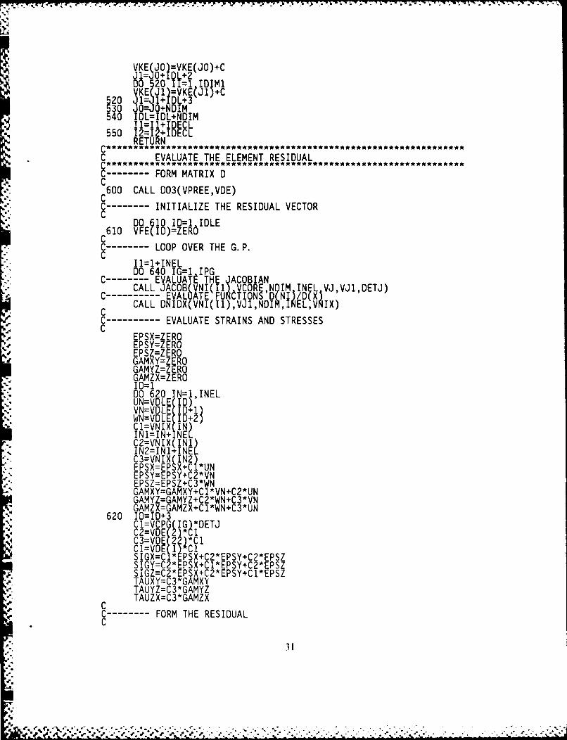
C EVALUATE THE ELEMENT RESIDUAL

CC ~ 600 CALL 003(VPREE,VDE)

C C-------- INITIALIZE THE RESIDUAL VECTORC

DO 610 ID=1 IDLEC610 VFE(ID)=ZEROC C-------LOOP OVER THE G. P.C

Il11+INELDO 640 IG=1 IPG

C ------- EVALUAT~ THE JCBACALL JACOB VNI(U) VCORE,N IM IN L VJ,VJ1 ,DETJ)

C---------EVALUATEFUNCTIONS D NI /D( X~C CALL DNIOX( VNI ( I),VJ1,NDIM,IEL,VNIX)

C --------- EVALUATE STRAINS AND STRESSESC

- EPSX=ZEROEPSY=ZEROEPSZ=ZEROGAMXY=ZEROGAMY Z=Z EROGAMZX=ZERO0062 I=J.,IEDNOLE20 ID),IEVN=VDLE (1+1)WN=VDLE (10+2)C1=VNIX (IN)IN1=IN+ NELC2=VNIX (INI)IN2=IN1 INEC3=VNIX I N2)EPSX=EPSX+C 1*UNEPSY=EPSY+C2*VNEPSZ=EPSZ+C3*WNGAMXY=GAMXY+C 1*VN+C2*UNGAMYZ=GAMYZ+C2*WN+C3*VNGAMZX=GAMZX+C1*WN+C3*UN

620 10=10+3C1=VCP( I G) *DETJC2=VDE( * IC3=VOE 2 )*C 1

ClVE1 *ClSIX= *PS X+C2 *EP SY+C2 *EPSZ

SIGY=C2*EPSX+Cl*EPSY+C2*EPSZSIGZ=C2*EPSX+C2*EPSY+Cl*EPSZTAUXY=C3*GAMXYTAUYZ=C3*GAMYZTAUZX=C3*GAMZX

CC -------- FORM THE RESIDUALC

31

q4,

' O0 IN= ,INELC1=VNIX (IN)IN1=IN+ [NELC2=VNIX( Ii)1N2=IN1 I NELC3= VNIJ 2 ( IN2) CVFE (ID )=Y FE (ID+C*SIGX+C2*TAUXY+C3*TAUZXVFEI 0+1 -V E(ID+11)+C2*SIGY+Cl*TAUXY+C3*TAUYZ

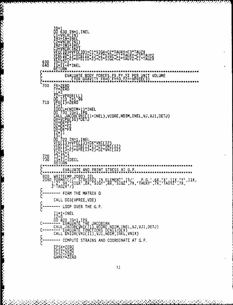
63 FE~ 0+2 )VE(D+2 )+C3*SIGZ+C2*TAUYZ+Cl*TAUZX6 0D=0D+3640 Il=I1+4*INEL

RETURNC EVALUATE BODY FORCES, FX,FY FZ PER UNIT VOLUMEC FOR GRAVITY FX=O FY=0 Z

700 FX=ZEROFY=Z EROL L=3FZ=-VPREE(LL

710 F ZR

IDECL=(NOIM+1 )*INEL00 730 IG= $ IPOCALL JACOB ~'Il+INEL),VCORE,N0IM,INEL,VJ,VJI,0ETJ)DX= CPG , IGOIJ

OZ=DX*FZ0X=DX*FX12=I113=1DO 720 INI1IN LVFE( 13)=VFE I3 +0X*VNIQI2)VFE( 13 +1)=VE 31)+OY VNI 12)VFE 13+2)=VFE(I3+2) +DZ*VNI 1

720 13=I3+3730 I1=I1+IDECL

RETURN

C EVALUATE AND PRINT STRESS AT G. P.

800 WREL ' MX 'Y',11X,2080 FORMA (// SIYN ELMN 1 1 PG:6 i .ll'Z' , s, I TXOZ 9X 'SIGX ,8X, S Y8XS T 7:X

2'TAOZX'/)C-----OMTEMTIC ---- OMTEMTI

CAL03VREVEC ALD)(VREVE

C-----OPOE H .PC-----LO OVRTEGP

* I1=+INEI2=0+NEDO120 I P

C----E0 UT THE JACOBIANCALL JACO VI(i CR NO IM INEL,VJ,VJ1,DETJ)

C ------- EVALUATE FUNCTONS D NIM/OXC CALL DNIDX(VNI(I1),VJ1,NDIM,INL,VNIX)

C ------- COMPUTE STRAINS AND COORDINATE AT G. P.C

EPSX=ZEROEPSY=ZEROEPSZ=ZEROGAMXY=ZERO

* 32

b - - I. - - a

GAMZ=ZEROGX=Z EROX=ZEROY=ZERO

00 810 1N= ,INELUN=VDLE~ ID)lWN=V LE 0+fXN=VCOR ID)YN=VCORE(01ZN=VCORF (I3+2)Cl1VN IX ININ1=IN+ INC2=VNIX (IN i)

I 1N2=IN1+I NE IC3=VNIX( 1N2)IN1=IN+i 2C4=VNI (INi)EPSX=E PSX+ C1"*UNEPSY=EPSY+C2*VNEPSZ=EPSZ+C3*WNGAMXY=GAMXY+Cl1*VN+C2*UNGAMYZ=GAMYZ+C2*WN+C3*VNGAMZX=GAMZX+C1*WN+C3*UNX=X+C4*XN

4=+4Y

Z=Z+C4*ZN810 10=10+3CC --------- COMPUTE THE STRESSESC

SIGX=VDE 1 *EPSX+VDE 2 *EPSY+VDE (2)*EPSZSIGY=V0E 2 *EPSX+VDE 1 *EPSY+VDE (2) *EPSZSIGZ=VDE ;* PSX+VDE (2) *EPSY+VOE (1) *EPSZTAUXY=VD MXY

TAUY=VD 22*GAMYTAUZX=VDE 22 *GAMZXWRITE MP 0 IGX YZSIGX,SIGY,SIGZ,TAUXY,TAUYZ,TAUZX

2090 FORMAT~ 09%,~8012=I2+ *INEL 2.580I1=Il+4*INEL

RETURNENDTUOUTNE

C TO EVALUATE THE SHAPE FUNCTIONS N AND THEIR DERIVATIVES W.R.T.C KSI,ETA,DZETAC INPUTC VKPG(NN)= COORDINATES OF POINTS IN KSI,ETA,DZETAC OUTPUTC V NI = THE SHAPE FUNCTION N ANDC THE DERIVATIVE OF SHAPE FUNCTION W.R.T. KSI ETA OZETA

IMPLICIT REAL*8 (A-H O-Z)DIMENSION VN 1(3456) ,CORR F(32 3' VKP(1,N3,)R(*DATA (CORRF(1 J), =1 3) 1=1 ' P(1)V(23)R(2

* /-i.60 -1 DO -1.0D:-. 33333333333333,-l.DO -1 DO 0.3333*33333333333,.1.O -*i DO 1.DO,-1.DO -1.00 1 DO -.333313333D~3333*-.OlD 33333 33 333 3 -1 DO i" DO 1'0b,-i.DO 33333333333331 1.0 -i.DO*-.3333333333333A3,!.D6 - b.o'-i.DOl O.b -1.00D -1i* DO

*O.3333333 333,..D,.D0-.332 33333 33 331. 00,b-1. 0o -1 b*-. 333333333333333 1 00 -1 D0 -.333333333333333,1.00 1 DO'-. 33j33*33333333 -1 00 1 00 - h3333333333 -1 DO -1 DO 3 33h33333333

33' 333:A3 33,1001 1iDbo .0 333 333333 3,ol. D00'**333333333333333 -1 DO b 001.D0,- i DO 1 DO 1 DO,-.3 33j333333*1l.D,1.00.33333333 ,)331D,.b, lb0, O,.33333333333333

33

*100O 1 00 -333333333333333 1 DO 1 DO -1 00 1 00 1.00,-i. DO,.3333*3333333,.D,..D,. 33 3 3333333*31.OO/

C 00 1 * §3jCl WRITE §9) Il CORRF(I~) J=13C99 FORMAT 2X, 12,S(X ,E E2.6)13)

'JJ=100 10 NN= ,81,3

X=VKPG(NNiY=VKPG(NNN+1Z=VKPG( N+2

DO 100 l2

X1=CORRF( J,Y1=C0RRF~ J,Z1=CORRF J3CF1=9.DO 640CF5=19.0/.0RN~J=F* 1.0+XXli(l.O+Y*Y1)( 1.O+ *Z1 * CF2+X*X+Y*Y+Z* )

*VN( J"=F76' 0Y*l*.DO+Z*Z1) *(X*f + OXXYYZZ

*VN(J,2)=CF1i;1.0+X*X1)*(1. 0+Z*Zl)*(Y*(-CF2+X*X43. DO*Y*Y+Z*Z)

100 *VN(J,3)=CFl l.D3+X*Xl)*(1. 0O+Y*Y1)*(Z1*(-CF2+X*X+Y*Y+3. D0*Z*Z)

C ----------- NODE # :2,3,8,9,22,23,28,29

00 200 K=1 2IK=20*( K-ijD0 200 I= ,211=6*(I1 2+1KI T= I+ 1DO 200 J=II i TX1=CORRF( J,1)Zl=CORRF( J 3)CF1=81.0 /k4D0CF =1. 00/9. DORN J)-CF1*- 1. 0-X*X C +X*X 0 +Y*YN) l D0+Z'*Z13XX*VN Do2 =CCF~3 0 1*X*X**XF1)X .0+z

c200 VN J, CIZ*lD0-X*Xi*0C2+X*X1l * .D0+Y*Y1)

C ------------ AT MIOSIDEC ------------ NODE # :5,6,11,12,25,26,31,32C

00 300 K=1 24

IT=11+100 300 J=II ITXl CORRF(J,=I CRRF J,2Zi CORRF J3

RN(J)=CFC* 1.00+X*D 00-*Y *M +l 0+Z*ZVN( J 1)= CFI *L D *(1VN J: C1 ~1( o+x*Xi ' I.rDo+Z Z 1 -20DOYX 2-3.D0*Y*Y*Yl)

300 VN(J,3) 1CF* L1*(.0+X X )*(l~f.D.y y*(CF22Y*Y1)

C ---- --------- AT MIOSIDEC ---- --------- NODE # 13,14,15,16,17,18,19,20

34

A. C00 400 33pX1=CORRF 3~,jZ1=CORRF J2Y1=CORRF J3)RNIJ)= F *tl.D0+X X1)*1 nO+Y*Y1)1*0 Z* F2+Z*Z1)

40 VN J,2 =CF1*Y1* lDOo+X*Xl * .' -* * CF2+Z*Z140VN(J 3 1=CF1* 1.SO+X*X1)*(I OWYl)* Z -2.OO*Z* F2-3.DO*z*Z*Z1)DO 10 L=1 U(

410 JJI33 RN+NDO 420 K=1,3

DO 430 1=1 32VNI (33)=VN(I,K)

430 33=33+1420 CONTINUE10 CONTINUE

RETURNENDTUOUTNE D0 PE

C TO FORM MATRIX D ( 3 DIMESIONAL ELASTICITY)C INPUTC VPREE = ELEMENT PROPERTYC VPREE(1 = YOUNG'SMODULUSC VPREE(2) = POISSON'S RATIOC OUTPUTC VDE = MATRIX D

IMPLICIT REAL*8 (A-H O-Z)DIMENSION VPREEC 1,VbOE(3bDATA ZERO/O.OD/,UNi ODO/,DEUX/2. 000/E=VPREE( 1LL=2

C2=CI X U~ SUN+X)*(UN-DEUX*X))C3=C1*s(60N-DU X*X)/(DEUX*(UN.X))DO 10 3=1 36

10 VD J =ZEF 0VDE I =C1

-. VDE 2 =C2VDE 3 =C2VOE 7 =C2VUE 8 =ClVD 9 =C2VOE 11 =C2VDE 14 =C2VDE 15 =C1VDE 22 =C3VDE 29 =C3VOE 361=C3RET RNENDSUBROUTINE BO3 V NIX INEL VBE *******************

C TO FORM MATRIX B (3 DIMEMSIONAL ELASTICITY)C INPUTC VNIX =DERIVATIVES OF SHAPE FUNCTION W.R.T. X,Y,ZC OUTPUTC VBE MATRIX B

/ IYPLIZIT REAL*8 (A-HOZDIMENSION VNIX(3 ,1),BE(61DO 10 I=1,600DO3 96

C 10 VBE\ I,3)=6.0DO

.115

C FORMATION OF MATRIX BCDO 20 I=1,32I1=3*I-212=11+113=12+1KK:IC2=VIXC2V X I =K2

VBE 2,12 =C2VBE 3, 3 =C3VBE 4,11 =C2VBE 4, 2 =C1VBE 5,12 =C3VBE 5,13 =C2VBE 6,11 =C3

20 VBE 6 131=ClRETORAENDSUBROUTINE BTDB(VKE VBF VDE IDLE IMATD,NSYM)

C TO ADD THE PRODUCT B(i).D.B TO THE ELEMENT MATRIX KC INPUTC VBE = MATRIX BC VDE = MATRIX DC OUTPUTC VKE = ELEMENT MATRIX K

IMPLICIT REAL*8 (A-H O-ZDIMENSION VKE(1),VBE(IMATD,I),VDE(IMATD,1),T(576)DATA ZERO/0.0 D0/IJ=1IMAX=IDLEDO 40 J=IIDLEDO 20 II=I,IMATDC=ZERODO 10 JI=IIMATD0~10 (I=C=C+VDE(II'JI)*VBE(JI'J)

CIER I(NSYM. EQ.,O) IMAX=JDo 40 I=I,IMAXC=ZERODO 30 JI=i,IMATD

30 C=0+VBE(JI *T(JI)VKE(IJ)=VKE(IJ)+C

40 IJ=IJ+RETURNEND

,.,,

4/

.4..

36]'a.. .. .- - # . ., . . . . . . z . ' ' ' ' ' L,-' '''. " ' : '

.MA,, , * . -

LIST OF REFERENCES

1. Dhatt, Gouri and Touzot, Gilbert, The Finite Element Method Displayed, JohnWiley & Sons, 1984.

2. Bathe, Klaus and Wilson, Edward, Numerical Methods In Finite ElementAnalysis, Prentice Hall, 1976.

3. Budynas, Richard G., Advanced Strength And Applied Stress Analysis,McGraw-Hill Company, 1977.

......... ........ ........ .a. I. .

INITIAL DISTRIBUTION LIST

No. Copies

1. Defense Technical Information Center 2Cameron StationAlexandria, Virginia 22304-6145

2. Library Code 0142 2Navaflostgraduate SchoolMonterey, California 93943-5002

3. Department Chairman, Code 69Department Of Mechanical EngineeringNaval Post graduate SchoolMonterey, California 93943-5000

4. Professor Gilles Cantin, Code 69Ci 4Department Of Mechanical EngineeringNaval Postgraduate SchoolMonterey, California 93943-5000

5. LibraryRoyal Thai Naval AcademyParknam, Samutplakan, Thailand

6. LT Anan Sukaneevouth 3Nor-96, Naval let VillageSattahip, Chonburi, Thailand

38

, ' 4 ," ' -. ', ,

, .,..-.". , . - * , ,

/I 4!'

-a--- I/// / /

/

-~ K~~-