1

Machine Learning Overview

Sargur N. Srihari University at Buffalo, State University of New York

USA

2

Outline

1.  What is Machine Learning (ML)? 1.  As a scientific Discipline 2.  As an area of Computer Science/AI

2.  Core learning methods 1.  Supervised (Regression/Classification/Deep) 2.  Unsupervised (PCA, Clustering, Topic Models) 3.  Reinforcement

3.  Main drivers 1.  Mobile systems (big data) 2.  Personalization

Machine Learning as a Discipline •  Focused on two inter-related fundamental

scientific/engineering questions 1.  How can one construct computer systems that

automatically improve through experience? 2.  What are the statistical-computational-information-

theoretic laws that govern all learning systems •  Including computers, humans and organizations?

•  Machine learning is also important for highly practical computer software fielded across many applications

3

4

Machine Learning as Software Area •  Programming computers to:

– Perform tasks that humans perform well but difficult to specify algorithmically

•  Principled way of building high performance information processing systems – Probabilistic responses to queries—IR – Adaptive user interfaces, personalized

assistants (information systems) – Scientific/engineering applications

ML within AI •  ML has emerged as method of choice for

practical software for: – Computer vision – Speech recognition – Natural language processing – Robot control – Other applications

•  Far easier to train by showing examples of input-output behavior – Than manually anticipate response for every input

5

6

Example Problem: Handwritten Digit Recognition

•  Handcrafted rules will result in large no of rules and exceptions

•  Better to have a machine that learns from a large training set

•  Handwriting recognition cannot be done without machine learning!

Wide variability of same numeral

7

Most Successful Application of ML

•  Learning to recognize spoken words – Speaker-specific strategies for recognizing

primitive sounds (phonemes) and words from speech signal

– Neural networks and methods for learning HMMs for customizing to individual speakers, vocabularies and microphone characteristics

– Recently Google increased accuracy for Android by 25% Table 1.1

8

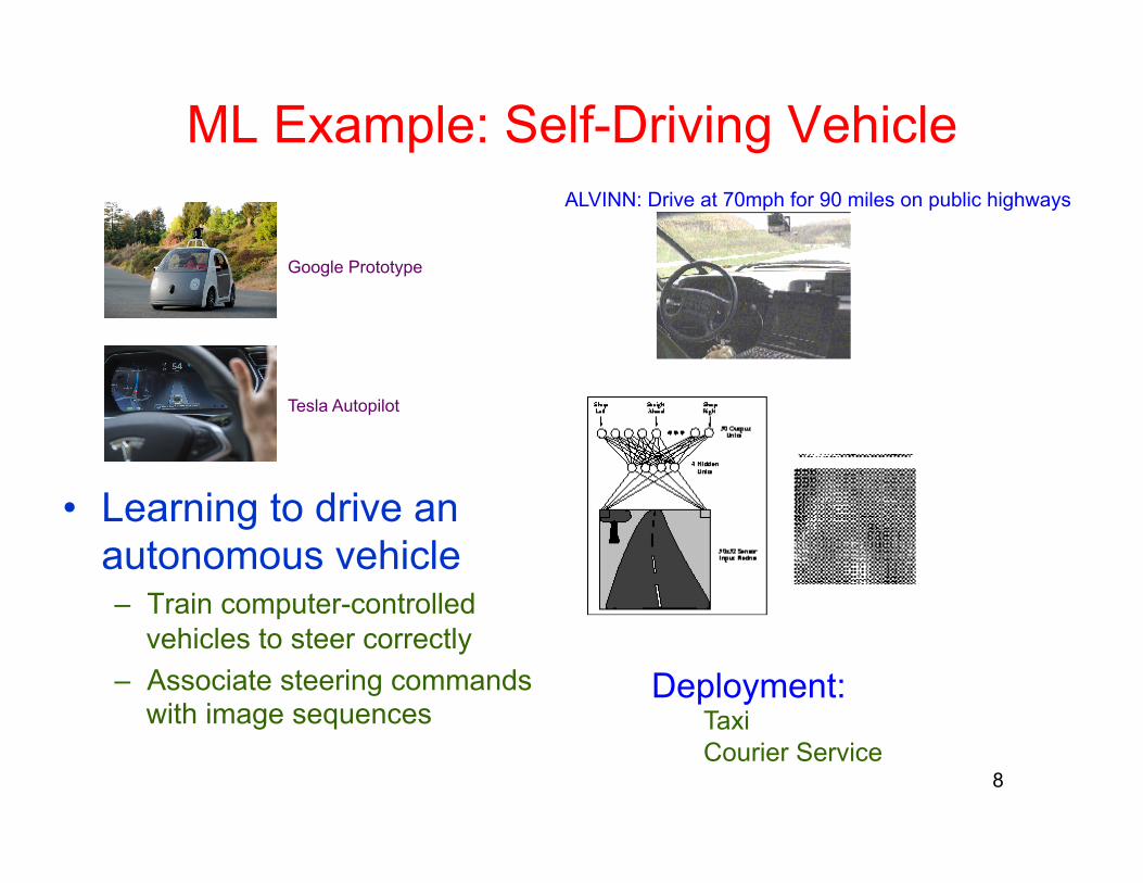
ML Example: Self-Driving Vehicle

•  Learning to drive an autonomous vehicle –  Train computer-controlled

vehicles to steer correctly –  Associate steering commands

with image sequences

Google Prototype

Deployment: Taxi Courier Service

ALVINN: Drive at 70mph for 90 miles on public highways

Tesla Autopilot

Drivers of ML Progress •  Mobile systems gather/transport vast

amounts of data: “Big data” – Turn to ML solutions to obtain insights,

predictions, decisions – Granularized personalized data

•  Personalization: relevance of posts shown –  Advertising copywriting

•  Historical medical records: Determine treatment •  Historical traffic data: Control congestion

9

Learning Problem Definition •  Improving some measure of performance P

when executing some task T through some type of training experience E

•  Example: Learning to detect credit card fraud

10

•  Task T–  Assign label of fraud or not fraud to credit card

transaction •  Performance measure P

–  Accuracy of fraud classifier With higher penalty when fraud is labeled as not fraud

•  Training experience E–  Historical credit card transactions labeled as fraud or not

11

The ML Approach

Generalization

(Training)

Data Collection Samples

Model Selection Probability distribution to model process

Parameter Estimation Values/distributions

Inference Find responses to queries

Decision (Inference

OR Testing)

12

ML History within AI •  ML/PR Methods around for over 50 years

Core Methods

1.  Supervised Learning – Training data consists of (x,y) pairs – Goal is prediction y* for input x*

2.  Unsupervised Learning – Analysis of unlabeled data

3.  Reinforcement Learning – Training data inbetween supervised/unsupervised

•  Indication of whether action is correct or not •  Rewad signal may refer to an entire input sequence 13

Supervised Learning •  Most widely used methods of ML, e.g.,

•  Spam classification of email •  Face recognizers over images •  Medical diagnosis systems

•  Inputs x are vectors or more complex objects – documents, DNA sequences or graphs

•  Outputs are binary, multiclass(K), – Multi-label (more than one class), ranking, – Structured:

•  y is a graph satisfying constraints, e.g., POS tagging – Real-valued or mixture of discrete and real-valued 14

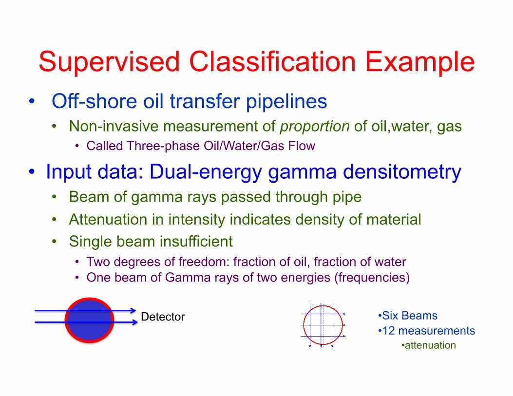
Supervised Classification Example •  Off-shore oil transfer pipelines

•  Non-invasive measurement of proportion of oil,water, gas •  Called Three-phase Oil/Water/Gas Flow

•  Input data: Dual-energy gamma densitometry •  Beam of gamma rays passed through pipe •  Attenuation in intensity indicates density of material •  Single beam insufficient

•  Two degrees of freedom: fraction of oil, fraction of water •  One beam of Gamma rays of two energies (frequencies)

Detector • Six Beams • 12 measurements

• attenuation

16

Prediction Problems 1.  Predict Volume Fractions of oil/water/gas 2.  Predict configuration (one of three)

–  Twelve Features –  Three classes –  Two variables, 100 points shown

Which class should x belong to?

•  Naïve cell based voting fails –  exponential growth of cells with

dimensionality –  12 dimensions discretized into 6

gives 3 million cells •  Hardly any points in each cell

17

Probability Theory •  Sum Rule for Marginalization •  Product Rule: for combining •  Bayes Rule

•  Fully Bayesian approach

•  Conjugate distributions •  Feasible with increased computational power •  Intractable posterior handled using either

–  Variational Bayes or –  Stochastic sampling –  e.g., Markov Chain Monte Carlo, Gibbs

p(X,Y ) =

nij

N= p(Y | X)p(X)

p(X = x

i) = p(X = x

i,Y = y

j)

j=1

L

∑

)()()|()|(

XpYpYXpXYp = ∑=

YYpYXpXp )()|()(where

Viewed as Posterior α likelihood x prior

18

Probability Distributions Discrete- Binary

Discrete- Multi-valued

Continuous

Bernoulli Single binary variable

Multinomial One of K values = K-dimensional binary vector

Gaussian

Angular Von Mises

Binomial N samples of Bernoulli

Beta Continuous variable between {0,1]

Dirichlet K random variables between [0.1]

Gamma ConjugatePrior of univariate Gaussian precision

Wishart Conjugate Prior of multivariate Gaussian precision matrix

Student’s-t Generalization of Gaussian robust to Outliers Infinite mixture of Gaussians

Exponential Special case of Gamma

Uniform

N=1 Conjugate Prior

Conjugate Prior

Large N

K=2

Gaussian-Gamma Conjugate prior of univariate Gaussian Unknown mean and precision

Gaussian-Wishart Conjugate prior of multi-variate Gaussian Unknown mean and precision matrix

19

Statistical Models •  Generative

–  Naïve Bayes –  Mixtures of

multinomials –  Mixtures of Gaussians –  Hidden Markov Models

(HMM) –  Bayesian networks –  Markov random fields

•  Discriminative –  Logistic regression –  SVMs –  Traditional neural

networks –  Nearest neighbor –  Conditional Random

Fields (CRF)

HMMs for Speech Recognition •  Three distinct layers 1.  Language Model:

– generates sentences as sequences of words

2.  Word Model: – described as a sequence of

phonemes /p//u//sh/ 3.  Acoustic model:

– shows progression of the acoustic signal through a phoneme 20

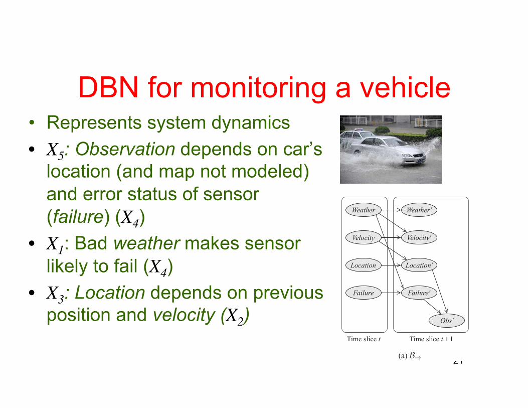
DBN for monitoring a vehicle •  Represents system dynamics •  X5: Observation depends on car’s

location (and map not modeled) and error status of sensor (failure) (X4)

•  X1: Bad weather makes sensor likely to fail (X4)

•  X3: Location depends on previous position and velocity (X2)

21

Obs0

Weather0

Velocity0

Location0

Failure0

Obs0

Weather0

Velocity0

Location0

Failure0

Obs1

Weather1

Velocity1

Location1

Failure1

Obs2

Weather2

Velocity2

Location2

Failure2

Obs'

Weather Weather'

Velocity Velocity'

Location Location'

Failure Failure'

(c) DBN unrolled over 3 steps(b) 0(a) →

Time slice t Time slice t +1 Time slice 0 Time slice 0 Time slice 1 Time slice 2

Regression

22

Problem data set

Red curve is result of fitting a two-layer neural network by minimizing squared error

Corresponding inverse problem by reversing x and t

Very poor fit to data: GMMs used here

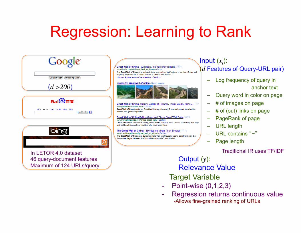
Regression: Learning to Rank

–  Log frequency of query in anchor text –  Query word in color on page –  # of images on page –  # of (out) links on page –  PageRank of page –  URL length –  URL contains “~” –  Page length

Input (xi): (d Features of Query-URL pair)

Output (y): Relevance Value

In LETOR 4.0 dataset 46 query-document features Maximum of 124 URLs/query

(d >200)

Target Variable

-  Point-wise (0,1,2,3) -  Regression returns continuous value

- Allows fine-grained ranking of URLs

Traditional IR uses TF/IDF

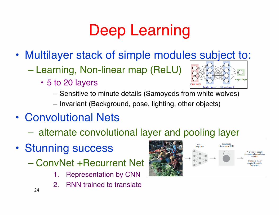
Deep Learning•  Multilayer stack of simple modules subject to:

– Learning, Non-linear map (ReLU)•  5 to 20 layers

–  Sensitive to minute details (Samoyeds from white wolves)–  Invariant (Background, pose, lighting, other objects)

•  Convolutional Nets–  alternate convolutional layer and pooling layer

•  Stunning success– ConvNet +Recurrent Net

1.  Representation by CNN2.  RNN trained to translate

24

Unsupervised Learning •  Labeled data under assumption of underlying

structure of data, e.g., 1.  Clustering is to find partition of data 2.  Identify a low-dimensional manifold

•  PCA, manifold learning, factor analysis, random projections, auto-encoders

•  Topic modeling, Recommendation systems

•  A criterion function is used e.g., max likelihood •  Computational complexity is key

–  to exploit large unlabeled data sets 25

26

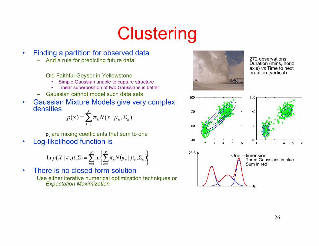
Clustering •  Finding a partition for observed data

–  And a rule for predicting future data

–  Old Faithful Geyser in Yellowstone •  Simple Gaussian unable to capture structure •  Linear superposition of two Gaussians is better

–  Gaussian cannot model such data sets •  Gaussian Mixture Models give very complex

densities

pk are mixing coefficients that sum to one •  Log-likelihood function is

•  There is no closed-form solution Use either iterative numerical optimization techniques or

Expectation Maximization

∑=

Σ=K

kkkk xNp

1

),|()x( µπ

One –dimension Three Gaussians in blue Sum in red

( )∑ ∑= = ⎭

⎬⎫

⎩⎨⎧ Σ=Σ

N

n

K

kkknk NXp

1 1

,|xln),,|(ln µπµπ

272 observations Duration (mins, horiz axis) vs Time to next eruption (vertical)

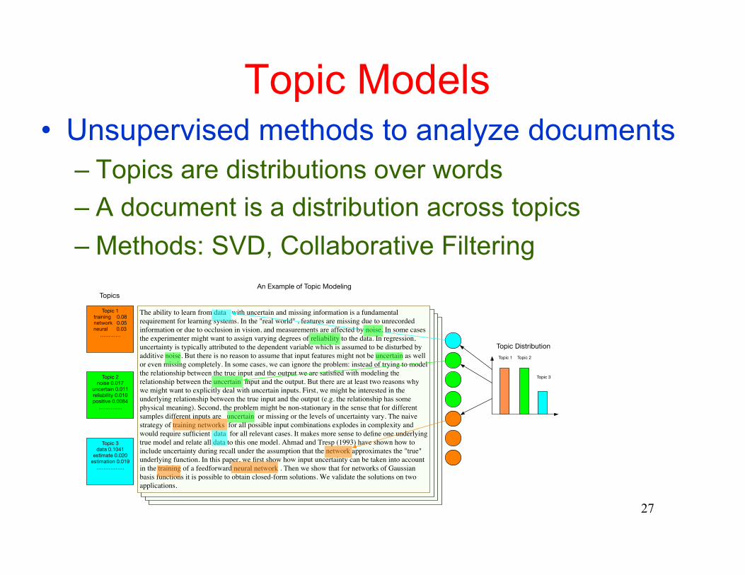
Topic Models •  Unsupervised methods to analyze documents

– Topics are distributions over words – A document is a distribution across topics – Methods: SVD, Collaborative Filtering

27

The ability to learn from data with uncertain and missing information is a fundamental requirement for learning systems. In the "real world" , features are missing due to unrecorded information or due to occlusion in vision, and measurements are affected by noise. In some cases the experimenter might want to assign varying degrees of reliability to the data. In regression, uncertainty is typically attributed to the dependent variable which is assumed to be disturbed by additive noise. But there is no reason to assume that input features might not be uncertain as well or even missing completely. In some cases, we can ignore the problem: instead of trying to model the relationship between the true input and the output we are satisfied with modeling the relationship between the uncertain input and the output. But there are at least two reasons why we might want to explicitly deal with uncertain inputs. First, we might be interested in the underlying relationship between the true input and the output (e.g. the relationship has some physical meaning). Second, the problem might be non-stationary in the sense that for different samples different inputs are uncertain or missing or the levels of uncertainty vary. The naive strategy of training networks for all possible input combinations explodes in complexity and would require sufficient data for all relevant cases. It makes more sense to define one underlying true model and relate all data to this one model. Ahmad and Tresp (1993) have shown how to include uncertainty during recall under the assumption that the network approximates the "true" underlying function. In this paper, we first show how input uncertainty can be taken into account in the training of a feedforward neural network . Then we show that for networks of Gaussian basis functions it is possible to obtain closed-form solutions. We validate the solutions on two applications.

Topic 1training 0.08network 0.05

neural 0.03…………

Topic 2noise 0.017

uncertain 0.011reliability 0.010positive 0.0084

…………..

Topic 3data 0.1041

estimate 0.020estimation 0.019

…………….

Topic 1 Topic 2

Topic 3

An Example of Topic Modeling Topics

Topic Distribution

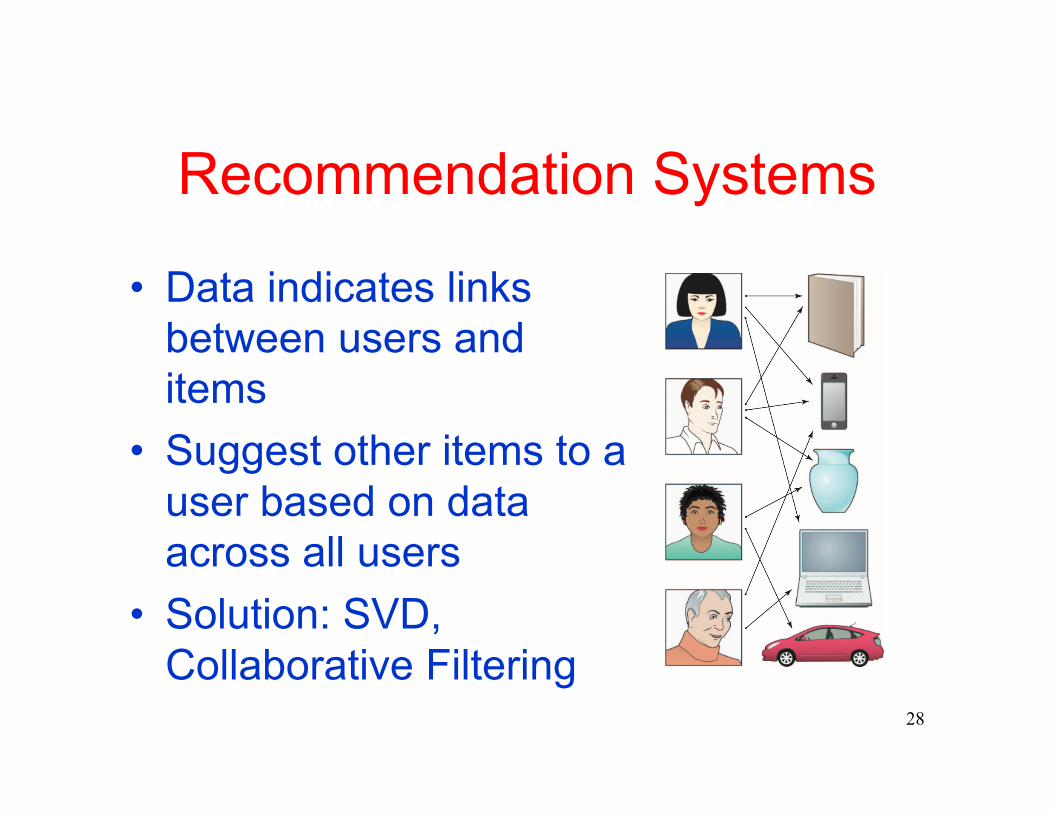
Recommendation Systems

•  Data indicates links between users and items

•  Suggest other items to a user based on data across all users

•  Solution: SVD, Collaborative Filtering

28

Reinforcement Learning

•  Dog is given a reward/punishment for an action –  Policies: what actions to take in a particular situation –  Utility estimation: how good is state (àused by policy)

•  No supervised output but delayed reward •  Credit assignment

– what was responsible for outcome •  Applications:

–  Game playing –  Robot in a maze –  Multiple agents, partial observability, … 29

Causal Learning

30

•  A Causal Bayesian Network •  Example of Inference:

Cancer is independent of Age and Gender given exposure to Toxics and Smoking

•  Computationally feasible inference

31

Summary •  Machine Learning Discipline

–  Study how systems improve with experience –  Study statistical-computational-information-theoretic laws

governing learning systems –  Used with success in all AI applications

•  Core methods: –  Supervised

•  Classification, Regression, Ranking –  Fully Bayesian approach together with Variational methods and Monte Carlo

sampling •  Deep Learning

–  Unsupervised (PCA, Topic Models, Clustering) –  Reinforcement

•  Drivers are mobile systems (big data), personalization