Embed Size (px)
Citation preview
UNIVERSIDADE DE BRASÍLIA - UnB
FACULDADE UNB DE PLANALTINA - FUP
PROGRAMA DE PÓS-GRADUAÇÃO EM CIÊNCIAS AMBIENTAIS
MAÍSA CARVALHO VIEIRA
PADRÕES ESPAÇO-TEMPORAIS DO ZOOPLÂNCTON EM UM
RESERVATÓRIO HIDRELÉTRICO TROPICAL
Orientador: Prof. Dr. Ludgero Cardoso Galli Vieira
Co-orientador: Prof. Dr. Luiz Felipe Machado Velho
PPG-Ciências Ambientais
Linha de Pesquisa: Manejo e conservação de recursos naturais
Brasília/DF-2017

UNIVERSIDADE DE BRASÍLIA - UnB
FACULDADE UNB DE PLANALTINA - FUP
PROGRAMA DE PÓS-GRADUAÇÃO EM CIÊNCIAS AMBIENTAIS
MAÍSA CARVALHO VIEIRA
PADRÕES ESPAÇO-TEMPORAIS DO ZOOPLÂNCTON EM UM
RESERVATÓRIO HIDRELÉTRICO TROPICAL
Dissertação apresentada como requisito para a obtenção
do título de Mestre em Ciências Ambientais no Programa
de Pós-Graduação em Ciências Ambientais da
Universidade de Brasília.
Orientador: Prof. Dr. Ludgero Cardoso Galli Vieira
Co-orientador: Prof. Dr. Luiz Felipe Machado Velho
PPG-Ciências Ambientais
Linha de Pesquisa: Manejo e conservação de recursos naturais
Brasília/DF-2017

Carvalho Vieira, Maísa
CV658p Padrões espaço-temporais do zooplâncton em um reservatório
hidrelétrico tropical / Maísa Carvalho Vieira; orientador
Ludgero Cardoso Galli Vieira; co-orientador Luiz Felipe
Machado Velho. -- Brasília, 2017.
63 p.
Dissertação (Mestrado - Mestrado em Ciências Ambientais)
- Universidade de Brasília, 2017.
1. Zooplâncton. 2. Reservatório hidrelétrico. 3. Estra-tégias para o biomonitoramento. 4. Sincronia espacial.
5. Amazônia. I. Vieira, Ludgero Cardoso Galli , orient. II.
Velho, Luiz Felipe Machado, co-orient. III. Título.

iv
AGRADECIMENTOS
Em primeiro lugar, agradeço a minha família por ter investido e acreditado no meu
sucesso pessoal, além de me ensinar a enfrentar os desafios da vida e aprender com os erros.
Às minhas amigas do curso de biologia “saudades ueg #sqn”, que fizeram parte do
meu dia-a-dia e compartilharam comigo momentos bons e ruins durante a graduação.
Aos meus amigos da Zara, que mesmo hoje em dia não convivemos mais diariamente,
foram fundamentais pois me incentivaram muito seguir meu sonho e entrar no mestrado.
Aos amigos que fiz em Planaltina-DF, principalmente aqueles que convivi nesses dois
últimos anos no NEPAL.
À Coordenação de Aperfeiçoamento de Pessoal de Nível Superior (CAPES), pelo
apoio financeiro.
Ao meu orientador Ludgero C. G. Vieira, por ser exemplo de profissional, pelo suporte
e acessibilidade ao me orientar.
Ao meu coorientador, Luiz Felipe Machado Velho, pelo auxílio de dados e
contribuição ao longo desses dois anos.
Em especial ao Luis Maurício Bini, pelas valiosas contribuições e pesadelos (kkk).
Aos professores membros da Banca Examinadora que aceitaram participar da
avaliação deste trabalho.
Para as pessoas que esperavam nomes citados, já vou me desculpando, mas se eu
citasse eu tenho certeza que esqueceria algum nome e não queria cometer de forma algum
esse tipo de erro. Não sou muito boa com palavras bonitas, mas agradeço de coração todas as
pessoas que me ajudaram diretamente ou indiretamente, sintam-se abraçados.
Queria agradecer por último, e não menos importante, ao meu namorido Hugo e a
Deus, por estarem presente no meu dia-a-dia e ouvirem minhas lamentações e minhas vitórias.
Sumário
APRESENTAÇÃO GERAL ..................................................................................................... 4
REFERÊNCIAS ..................................................................................................................... 6
SINCRONIA ESPACIAL DO ZOOPLÂNCTON E DAS VARIÁVEIS AMBIENTAIS LIMNOLÓGICAS
DURANTE O REPRESAMENTO DE UM RESERVATÓRIO TROPICAL
RESUMO ............................................................................................................................. 9
INTRODUÇÃO...................................................................................................................... 9
MATERIAIS E MÉTODOS ................................................................................................... 11
RESULTADOS .................................................................................................................... 15
DISCUSSÃO....................................................................................................................... 19
CONCLUSÃO ..................................................................................................................... 21
REFERÊNCIAS ................................................................................................................... 22
MATERIAL SUPLEMENTAR (I)........................................................................................... 27
BIODIVERSITY SHORTCUTS IN BIOMONITORING OF NOVEL ECOSYSTEMS
ABSTRACT ........................................................................................................................ 29
INTRODUCTION................................................................................................................. 29
MATERIALS AND METHODS ............................................................................................. 31
RESULTS .......................................................................................................................... 33
DISCUSSION ..................................................................................................................... 39
CONCLUSION .................................................................................................................... 42
REFERENCES .................................................................................................................... 42
SUPPLEMENTARY MATERIAL (II) ..................................................................................... 50
4
APRESENTAÇÃO GERAL
Ambientes aquáticos são excelentes modelos para a observação de padrões e processos
ecológicos, pois estão sujeitos à grandes variações ambientais e biológicas, tanto ao longo do
espaço como ao longo do tempo (Fernandes et al., 2013; Leibold et al., 2004). Ecossistemas
aquáticos naturais estão entre os ambientes mais ameaçados do mundo (Dudgeon et al., 2006),
destacando os rios, que tem seus cursos muitas vezes represados para atender uma demanda
social energética (Nilsson et al., 2005). Há um crescimento contínuo no número de
reservatórios em países em desenvolvimento, particularmente reservatórios hidrelétricos
(Simões et al., 2015). Reservatórios hidrelétricos são fundamentais não apenas para a
produção da energia, mas também para a pesca, abastecimento de água, irrigação e
pisciculturas (Julio Jr. et al., 2005; Kennedy et al., 2003). Por outro lado, geram grandes
impactos ambientais, muitos irreversíveis, como a perda de biodiversidade (Andrade and Dos
Santos, 2015; Dudgeon et al., 2006).
As mudanças na dinâmica hidrológica, de um ambiente lótico para lêntico, decorridas
do represamento, geram modificações físicas, químicas e biológicas que afetam a estrutura
das comunidades (Simões et al., 2015). Por exemplo, maior entrada de matéria orgânica
advindas de inundações de árvores, deslocamento de populações, perda de valores estéticos,
redução das vazões a jusante do reservatório e aumento em suas variações, entre outros
(Tundisi and Matsumura-Tundisi, 2008; Emery et al. 2015). Essas modificações alteram em
especial às comunidades planctônicas (Silva et al., 2014), como o zooplâncton. O zooplâncton
é constituído por diferentes grupos taxonômicos (e.g. amebas testáceas, rotíferos e
microcrustáceos) com ciclos de vida distintos (Bonecker et al., 2013), e que respondem
rapidamente às mudanças ambientais, por terem um ciclo de vida rápido, além de terem
grande importância na cadeia trófica (Simões et al., 2015).
Algumas flutuações através do espaço e tempo são notáveis em todas as populações
(Heino et al., 1997), inclusive nas zooplanctônicas (Lansac-Tôha et al., 2008; Lodi et al.,
2014). Um desses padrões é a sincronia espacial, que é uma co-variação positiva no tamanho
populacional de diferente espécies (Descamps et al., 2013). Alguns fatores podem atuar
sincronizando as populações, sendo eles intrínsecos e extrínsecos. Os intrínsecos, são aqueles
que ocorrem dentro do reservatório hidrelétrico, como as variáveis ambientais limnológicas e
a dispersão dos organismos, e os extrínsecos, são aqueles que ocorrem fora do reservatório,
como o clima e precipitação (Bjørnstad et al., 1999; Ranta et al., 1997; Royama, 1992).

5
O estudo da sincronia pode auxiliar na otimização de programas de monitoramento
ambiental e/ou biológico, pois locais com alta sincronia podem ter menos pontos amostrados,
e o inverso é verdadeiro. Da mesma forma, a concordância entre grupos zooplanctônicos, ou
seja, quando um grupo pode substituir a amostragem de outro grupo sem perdas significati-
vas, e de diferentes arranjos de unidades de amostragem também podem auxiliar em progra-
mas de monitoramento, tanto em relação ao número de unidades amostrais quanto suas
localizações no espaço e no tempo (Rhodes and Jonzén, 2011). E para evitar e/ou minimizar
maiores impactos ambientais, perda de serviços e funções ecossistêmicas, são necessários
além do desenvolvimento de ações conservacionistas (Ceballos et al., 2015), a implantação de
eficientes programas de monitoramento ambiental (Kallimanis et al., 2012).
Assim, quando há necessidade de uma rápida avaliação dos ambientes e da
identificação precisa de impactos negativos sobre a biota advindos de um represamento por
exemplo, os métodos de substituição de espécies (e.g grupos substitutos, resolução taxonômi-
ca e resolução numérica) podem ser utilizados em alguns casos, sem que haja perda
significativa de informações sobre o estado atual dos locais monitorados (Khan, 2006). Esses
métodos de substituição podem estar relacionados com padrões estruturais concordantes em
uma comunidade ou grupos taxonômicos distintos, em um mesmo conjunto de locais
semelhantes (Bini et al., 2008). Assim, o objetivo geral desse trabalho é compreender as
dinâmicas espaço-temporais das comunidades zooplanctônicas em um reservatório
hidrelétrico tropical, a fim de otimizar práticas em monitoramento ambiental.
Assim, no primeiro capítulo avaliamos a sincronia espacial nas populações biológicas
do zooplâncton e variáveis ambientais limnológicas durante a construção de um reservatório
hidrelétrico amazônico. E o segundo capítulo foi avaliar a suficiência taxonômica, nesse caso,
táxons em escalas grosseiras poderiam substituir táxons em escalas refinadas; resolução nu-
mérica, quando a riqueza de espécie poderia substituir dados de abundância de espécies; e
abordagem de grupos substitutos, quando um grupo zooplanctônico poderia substituir outro
grupo zooplanctônico, sendo essas avaliações em escalas espaço-temporais.
6
REFERÊNCIAS
Andrade, A.D.L., Dos Santos, M.A., 2015. Hydroelectric plants environmental viability:
Strategic environmental assessment application in Brazil. Renew. Sustain. Energy Rev.
52, 1413–1423. doi:10.1016/j.rser.2015.07.152
Bini, L.M., Caetano, L., Da Silva, F., Luiz, A., Velho, F.M., Bonecker, C.C., Lansac-Tôha,
F.A., 2008. Zooplankton assemblage concordance patterns in Brazilian reservoirs.
Hydrobiologia 598, 247–255. doi:10.1007/s10750-007-9157-3
Bjørnstad, O.N., Ims, R.A., Lambin, X., 1999. Spatial population dynamics: analyzing
patterns and processes of population synchrony. Trends Ecol. Evol. 14, 427–432.
Bonecker, C.C., Simões, N.R., Minte-Vera, C.V., Lansac-Tôha, F.A., Velho, L.F.M.,
Agostinho, Â.A., 2013. Temporal changes in zooplankton species diversity in response to
environmental changes in an alluvial valley. Limnol. - Ecol. Manag. Inl. Waters 43, 114–
121. doi:10.1016/j.limno.2012.07.007
Ceballos, G., Ehrlich, P.R., Barnosky, A.D., García, A., Pringle, R.M., Palmer, T.M., 2015.
Accelerated modern human–induced species losses: Entering the sixth mass extinction.
Sci. Adv. 1.
Descamps, S., Strøm, H., Steen, H., 2013. Decline of an arctic top predator: Synchrony in
colony size fluctuations, risk of extinction and the subpolar gyre. Oecologia 173, 1271–
1282. doi:10.1007/s00442-013-2701-0
Dudgeon, D., Arthington, A.H., Gessner, M.O., Kawabata, Z.-I., Knowler, D.J., Lévêque, C.,
Naiman, R.J., Prieur-Richard, A.-H., Soto, D., Stiassny, M.L.J., Sullivan, C.A., 2006.
Freshwater biodiversity: importance, threats, status and conservation challenges. Biol.
Rev. Camb. Philos. Soc. 81, 163–82. doi:10.1017/S1464793105006950
Emery, K.A., Wilkinson, G.M., Ballard, F.G., Pace, M.L., 2015. Use of allocthonous resources
by zooplankton in resorvoirs. Hydrobiologia 758, 257-269.
Fernandes, I.M., Henriques-Silva, R., Penha, J., Zuanon, J., Peres-Neto, P.R., 2013.
Spatiotemporal dynamics in a seasonal metacommunity structure is predictable: the case
of floodplain-fish communities. Ecography (Cop.). 37, no-no. doi:10.1111/j.1600-
0587.2013.00527.x
Heino, M., Kaitala, V., Ranta, E., Lindström, J., 1997. Synchronous dynamics and rates of
extinction in spatially structured populations. Proc. R. Soc. London B Biol. Sci. 264,
481–486. doi:10.1098/rspb.1997.0069
7
Julio Jr., H.F., Thomaz, S.M., Agostinho, A.A., 2005. Distribuição e caracterização dos
reservatórios, in: Rodrigues, L., Thomaz, S.M., Agostinho, A.A., Latini, J.D. (Eds.),
Biocenoses Em Reservatórios: Padrões Espaciais E Temporais. São Carlos, pp. 1–16.
Kallimanis, A.S., Mazaris, A.D., Tsakanikas, D., Dimopoulos, P., Pantis, J.D., Sgardelis, S.P.,
2012. Efficient biodiversity monitoring: Which taxonomic level to study? Ecol. Indic.
15, 100–104. doi:10.1016/j.ecolind.2011.09.024
Kennedy, R.H., Tundisi, J.G., Straškrábová, V., Lind, O.T., Hejzlar, J., 2003. Reservoirs and
the limnologist’s growing role in sustainable water resource management. Hydrobiologia
504, 1999–2000. doi:10.1023/B:HYDR.0000008470.25059.f2
Khan, A.S., 2006. Is species level identification essential for environmental impact studies?
Curr. Sci. 91, 29–34.
Lansac-Tôha, F.A., Bini, L.M., Velho, L.F.M., Bonecker, C.C., Takahashi, E.M., Vieira,
L.C.G., 2008. Temporal coherence of zooplankton abundance in a tropical reservoir.
Hydrobiologia 614, 387–399. doi:10.1007/s10750-008-9526-6
Leibold, M.A., Holyoak, M., Mouquet, N., Amarasekare, P., Chase, J.M., Hoopes, M.F., Holt,
R.D., Shurin, J.B., Law, R., Tilman, D., Loreau, M., Gonzalez, A., 2004. The
metacommunity concept: a framework for multi-scale community ecology. Ecol. Lett. 7,
601–613. doi:10.1111/j.1461-0248.2004.00608.x
Lodi, S., Velho, L.F.M., Carvalho, P., Bini, L.M., 2014. Patterns of zooplankton population
synchrony in a tropical reservoir. J. Plankton Res. 36, 966–977.
doi:10.1093/plankt/fbu028
Nilsson, C., Reidy, C., Dynesius, M., Revenga, C., 2005. Fragmentation and Flow Regulation
of the World â€TM s Large River Systems. Science (80-. ). 308, 405–408.
doi:10.1126/science.1107887
Ranta, E., Kaitala, V., Lundberg, P., 1997. The Spatial Dimension in Population Fluctuations.
Science (80-. ). 275, 1621–1623.
Rhodes, J.R., Jonzén, N., 2011. Monitoring temporal trends in spatially structured
populations: how should sampling effort be allocated between space and time?
Ecography (Cop.). 34, 1040–1048. doi:10.1111/j.1600-0587.2011.06370.x
Royama, T., 1992. Analytical Population Dynamics. Springer Netherlands, Dordrecht.
doi:10.1007/978-94-011-2916-9
Silva, L.H.S., Huszar, V.L.M., Marinho, M.M., Rangel, L.M., Brasil, J., Domingues, C.D.,
Branco, C.C., Roland, F., 2014. Drivers of phytoplankton, bacterioplankton, and
zooplankton carbon biomass in tropical hydroelectric reservoirs. Limnologica 48, 1–10.

8
doi:10.1016/j.limno.2014.04.004
Simões, N.R., Nunes, A.H., Dias, J.D., Lansac-Tôha, F.A., Velho, L.F.M., Bonecker, C.C.,
2015. Impact of reservoirs on zooplankton diversity and implications for the
conservation of natural aquatic environments. Hydrobiologia 758, 3–17.
doi:10.1007/s10750-015-2260-y
Tundisi, J.G., Matsumura-Tundisi, T., 2008. Represas artificiais. In: Limnologia. Oficina de
textos, pp. 320.
9
CAPÍTULO I
Manuscrito será submetido na Ecology.
(http://esajournals.onlinelibrary.wiley.com/hub/journal/10.1002/(ISSN)1939-9170/)
Sincronia espacial do zooplâncton e das variáveis ambientais limnológicas durante o
represamento de um reservatório tropical
Resumo
Reservatórios são ecossistemas artificiais que modificam a estrutura das populações
biológicas. Dessa forma, é necessário entender as dinâmicas populacionais desse tipo de
ambiente, como por exemplo, verificar se há ou não correlação temporal dos padrões de
distribuição espacial conhecida como sincronia espacial é dada como uma correlação entre a
mesma população biológica ou variável ambiental ao longo do tempo. Assim, verificamos se
há sincronia espacial nas populações biológicas e variáveis ambientais limnológicas durante a
implementação de um reservatório hidrelétrico tropical. Obtivemos valores síncronos tanto
para populações quanto para as variáveis ambientais limnológicas. A sincronia populacional
pode ser associada a algumas variáveis limnológicas, como as variáveis relacionadas com a
quantidade de nutrientes, e a sincronia ambiental pode estar relacionada a fatores extrínsecos,
como as variações climáticas. A sincronia é clara em nossos resultados, porém não
conseguimos identificar os mecanismos que estão atuando, indicando que mais de um fator
pode estar influenciando na dinâmica. Para melhor compreensão dos mecanismos atuantes na
dinâmica populacional e ambiental, sugerimos que além de usar as variáveis ambientais
limnológicas e fazer a sincronia espacial, deve-se usar dados meteorológicos e de paisagem.
Palavras-chaves: rio Jari, barragem, Amazônia, dinâmica populacional
Introdução
Um dos objetivos da ecologia de populações e comunidades é compreender as causas
e consequências da variação na abundância dos organismos ao longo do tempo (Stange et al.
2011). Assim, a dinâmica de populações através da correlação temporal dos padrões de
distribuição espacial vem sendo estudada como uma forma de avançar os estudos sobre os
padrões e processos ecossistêmicos (Liebhold et al. 2004).
A variação síncrona de caráter mensurável em populações, comunidades ou
10
ecossistemas é chamada de sincronia espacial, ou seja, a similaridade temporal em diferentes
populações distribuídas espacialmente, sendo, portanto uma covariação positiva nas
flutuações no tamanho da população (Descamps et al. 2013). Ela é usualmente calculada
como a correlação entre a mesma população através do tempo (Bjørnstad et al. 1999),
avaliando a estabilidade temporal de cada população ou comunidade. Diversos modelos
teóricos e empíricos mostram que populações naturais estão propensas a sincronia espacial,
como populações de roedores e seus predadores (Ims and Steen 1990), algas gigantes
(Cavanaugh et al. 2013), populações de galos silvestres (Cattadori et al. 2000), fitoplâncton
(Xu et al. 2009) e populações de zooplâncton (Seebens et al. 2013, Lodi et al. 2014, Buttay et
al. 2017).
Muitos estudos de sincronia espacial foram realizados com organismos planctônicos,
comparando suas dinâmicas populacionais entre vários lagos temperados (Rusak et al. 1999,
George et al. 2000, Baines et al. 2000, Arnott et al. 2003, Anneville et al. 2004, Seebens et al.
2013). Recentemente, estudos realizados em um único sistema, como reservatórios, tem
ganhado reconhecimento da comunidade científica (Lansac-Tôha et al. 2008, Xu et al. 2009,
2012, Lodi et al. 2014). Assim, é relevante direcionar nossas atenções aos ambientes que estão
sob este tipo de modificação, visto que a formação dos reservatórios pode promover
alterações temporais, verticais, laterais e longitudinais no curso natural dos rios (Baxter 1977,
Stanford and Ward 2001).
A sincronia pode ser obtida através de fatores extrínsecos, como os distúrbios globais
(i.e. variações ambientais correlacionadas) que influenciam na renovação da população
(Ostfeld and Keesing 2000, Liebhold et al. 2004). Existem outros processos como os
intrínsecos, ou seja, as variáveis ambientais limnológicas e processos dispersivos que podem
explicar uma parte considerável da correlação entre sincronia populacional e distância
espacial ou ambiental (Koenig 1999, Cavanaugh et al. 2013). Sendo assim, as correlações
negativas entre a distância e a sincronia indicam que a migração é importante para a sincronia
das populações vizinhas (Heino et al. 1997, Roche et al. 2016). Vários estudos separaram
fatores regionais (i.e. clima e precipitação) e a dispersão, como se fossem fatores
independentes um do outro (Tedesco et al. 2004), porém, eles podem interagir, sendo
complementares na explicação da sincronia das populações (Kendall et al. 2000, Liebhold et
al. 2004). Identificar quais mecanismos (fatores extrínsecos, dispersão ou ambiental local)
estão atuando na sincronia é um grande desafio (Downing et al. 2008, Descamps et al. 2013),
já que os mesmos podem apresentar diferentes formas de interação.
As implicações da sincronia espacial são muito importantes para a gestão de

11
populações, pois ela está diretamente relacionada com a probabilidade de extinção (Heino et
al. 1997). A explicação é simples, se uma população é síncrona, quando uma se extingue,
todas as outras são suscetíveis a ter o mesmo destino. Porém, se a sincronia é baixa, algumas
subpopulações são sujeitas a abundância e servem para reestabelecer subpopulações extintas
(Liebhold et al. 2004). Populações síncronas tem outras implicações significativas
principalmente para biomonitoramentos, pois ao ter um alto nível de sincronia espacial, o
esforço amostral seria menor, podendo ser monitoradas em poucos ambientes, além de
diminuir o tempo de amostragem e recursos financeiros (Rhodes and Jonzén 2011).
Assim, esse trabalho visa examinar a sincronia espacial de populações do zooplâncton
que possuem maior frequência e de variáveis ambientais limnológicas durante o período de
implementação de um reservatório hidrelétrico tropical. Esse trabalho pretende responder as
seguintes perguntas: i) Há mudanças na estruturação dos grupos zooplanctônicos nas fases de
construção do reservatório? ii) Existe sincronia populacional e ambiental? Em caso positivo,
essa sincronia ocorre em todas as fases da construção do reservatório? iii) A dinâmica
síncrona populacional de zooplâncton é influenciada pela estruturação ambiental e/ou
espacial? iv) a sincronia ambiental é definida pela distância espacial? Dessa forma, esperamos
encontrar sincronia espacial principalmente após o represamento do rio, pois acreditamos que
o ambiente vai se homogeneizar ao passar de lótico para lêntico. Espera-se também que os
fatores locais atuem sincronizando as populações e as variáveis ambientais limnológicas, já
que o estudo foi realizado em um único ambiente e que os pontos amostrados são conectados
(Heino et al. 1997, Liebhold et al. 2004).
Materiais e Métodos
Área de Estudo
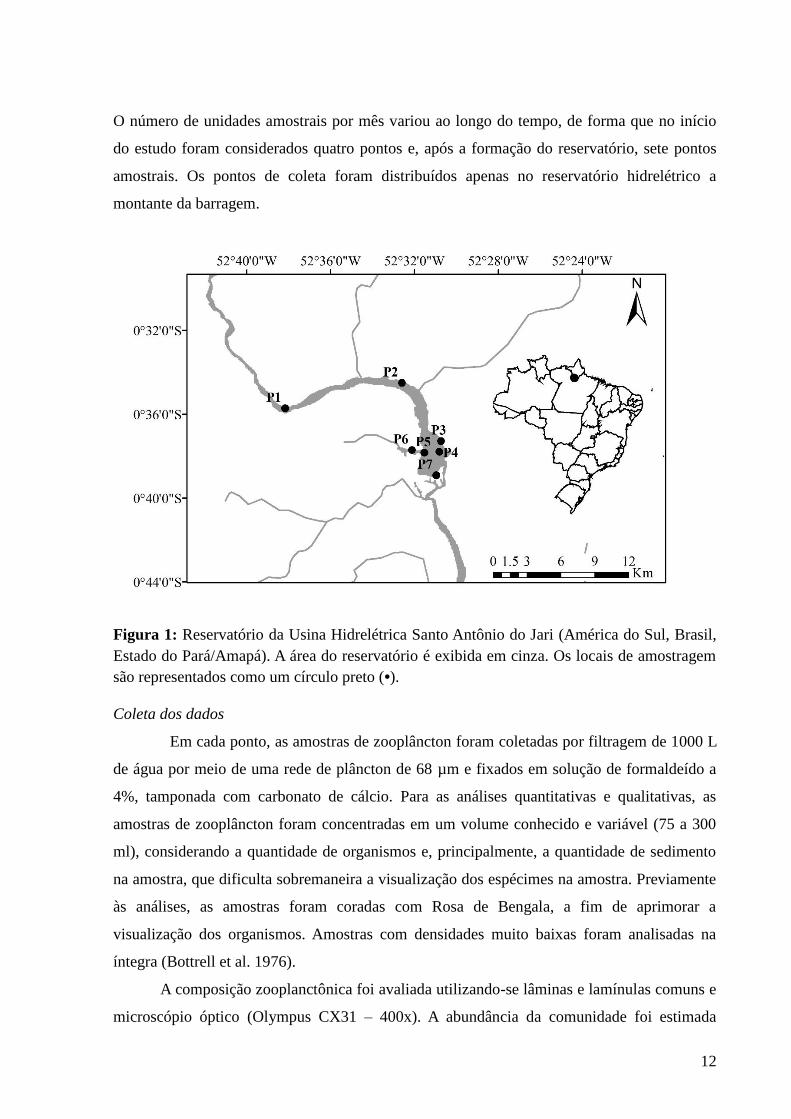
Esse estudo foi realizado no reservatório da Usina Hidrelétrica (UHE) Santo Antônio
do Jari (Figura 1). Essa UHE foi construída no período de 2011 a 2014 e está localizado no rio
Jari, tributário do rio Amazonas, na divisa dos estados do Pará e Amapá, Brasil (Filizola et al.
2002). O reservatório da UHE Santo Antônio do Jari apresenta uma área total de 31,7 km²,
volume de 133,39 x 10⁶ m³, profundidade média de 9,5 m e tempo de residência da água de
aproximadamente 1,5 dia (www.jarienergia.com.br). Foi realizada uma coleta por mês, em um
total de 23 meses, sendo nove meses na fase rio, portanto, antes do represamento efetivo
(fevereiro de 2012 a fevereiro de 2014), três meses na fase de transição rio-reservatório que é
no período de enchimento do reservatório (maio a julho de 2014) e onze meses na fase
reservatório, no qual a usina já estava em funcionamento (agosto de 2014 a agosto de 2015).
12
O número de unidades amostrais por mês variou ao longo do tempo, de forma que no início
do estudo foram considerados quatro pontos e, após a formação do reservatório, sete pontos
amostrais. Os pontos de coleta foram distribuídos apenas no reservatório hidrelétrico a
montante da barragem.
Figura 1: Reservatório da Usina Hidrelétrica Santo Antônio do Jari (América do Sul, Brasil,
Estado do Pará/Amapá). A área do reservatório é exibida em cinza. Os locais de amostragem
são representados como um círculo preto (•).
Coleta dos dados
Em cada ponto, as amostras de zooplâncton foram coletadas por filtragem de 1000 L
de água por meio de uma rede de plâncton de 68 µm e fixados em solução de formaldeído a
4%, tamponada com carbonato de cálcio. Para as análises quantitativas e qualitativas, as
amostras de zooplâncton foram concentradas em um volume conhecido e variável (75 a 300
ml), considerando a quantidade de organismos e, principalmente, a quantidade de sedimento
na amostra, que dificulta sobremaneira a visualização dos espécimes na amostra. Previamente
às análises, as amostras foram coradas com Rosa de Bengala, a fim de aprimorar a
visualização dos organismos. Amostras com densidades muito baixas foram analisadas na
íntegra (Bottrell et al. 1976).
A composição zooplanctônica foi avaliada utilizando-se lâminas e lamínulas comuns e
microscópio óptico (Olympus CX31 – 400x). A abundância da comunidade foi estimada

13
através da contagem, em câmaras de Sedgwick-Rafter, de 5 sub-amostras, de 1,5 ml (total de
7,5 ml), obtidas com pipeta do tipo Hensen-Stempell, sendo os resultados de densidade final
expressos em indivíduos por m-3.
Em cada amostragem, foram medidas in situ as seguintes variáveis ambientais
limnológicas: condutividade (potenciômetro digital Hanna), temperatura da água
(multiparâmetro YSI 556) e turbidez (turbidímetro digital Hach). Nos mesmos pontos de
coleta, amostras de água foram filtradas em membranas Whatman GF/C, que foram
armazenadas em freezer a –20ºC para posterior determinação das concentrações do material
em suspensão (Wetzel and Likens 2000), clorofila-a, fósforo total (Golterman et al. 1978) e
concentrações totais de nitrogênio (Mackereth et al. 1978).
Análise dos dados
Todas as análises foram realizadas no software estatístico R (R Development Core
Team 2017). Para isso, fez-se um conjunto de dados para cada variável analisada, seja ela
biológica ou ambiental, no qual a série temporal foi apresentada nas linhas e os pontos
amostrados nas colunas (Figura 2). Os dados biológicos foram classificados em nível de
espécie e grupos zooplanctônicos (cladóceros, copépodes, rotíferos e amebas testáceas).
Quando não foi possível a identificação a nível de espécies, os organismos foram
classificados ao nível de gênero ou família. As formas larvais e juvenis de copépodes foram
consideradas como entidades taxonômicas.
Uma Análise de Escalonamento Multidimensional Não-Métrico (NMDS) foi realizada
para visualização da composição dos grupos zooplanctônicos (cladóceros, copépodes,
rotíferos e amebas testáceas), ao longo da série temporal (23 meses), através da função
metaMDS. Os dados dos quatro grupos biológicos (ver Figura 2) foram submetidos a
padronização de Hellinger (função decostand - método hellinger) e a uma matriz de distância
de Bray-Curtis. Todas as funções dessas análises se encontram no pacote vegan (Oksanen et
al. 2016). Para avaliar se a similaridade da composição de grupos zooplanctônicos se
diferencia ao longo da série temporal entre as três etapas da implantação do reservatório (fase
rio, transição rio-reservatório e reservatório), fez-se uma Análise Multivariada Permutacional
de Variância (PERMANOVA, ver Anderson, 2001), usando matrizes de distâncias por meio
da função adonis do pacote vegan (Oksanen et al. 2016). Quando houve diferença
significativa nos grupos zooplanctônicos, fez-se novamente outra PERMANOVA, porém,
entre pares de fases do represamento para verificar entre quais fases estavam a diferença, por
exemplo, entre a fase rio e transição rio-reservatório ou entre a transição rio-reservatório e

14
reservatório. Os dados biológicos foram sempre transformados em log (x+1) para reduzir os
efeitos de valores extremos. Utilizou-se o coeficiente de Bray-Curtis como medida de
dissimilaridade com 5.040 permutações.
A sincronia é a média de uma matriz de correlação cruzada entre pares de pontos (i,j)
retirando a diagonal (Bjørnstad et al. 1999), dessa forma, para realizar a correlação cruzada é
necessário que os dados estejam dispostos da mesma forma da figura 2. Para minimizar a
quantidade de zeros nos dados biológicos, foram considerados apenas taxas com ocorrência
em mais de 25% de todos os pontos coletados (ou seja, em pelo menos 36 de 146 pontos ao
longo dos 23 meses de amostragem).
Estimou-se a sincronia populacional (B) através da média da correlação cruzada de
Spearman entre os pares de pontos de cada variável biológica (grupos e espécies do
zooplâncton). A significância do teste foi estimada por meio de 5.040 permutações de Monte
Carlo. Semelhantemente, a matriz de sincronia ambiental (E) foi estimada por meio da
correlação cruzada de Pearson com cada variável ambiental (temperatura, condutividade,
sólidos totais dissolvidos, turbidez, clorofila-a, fósforo total, nitrogênio total e demanda
química biológica). Todas as sincronias (B e E) foram realizadas por meio da função
meancorr do pacote synchrony (Gouhier and Guichard 2014). As análises de sincronia
populacional e ambiental foram realizadas para toda série temporal e para os três períodos do
reservatório (rio, rio-reservatório e reservatório), entretanto a sincronia populacional dos três
períodos foi testado apenas para os grandes grupos zooplanctônicos (cladóceros, copépodes,
rotíferos e amebas testáceas).
Para analisar o que poderia estar influenciando a sincronia populacional, estabeleceu-
se uma matriz de distância espacial (S) entre os pares de locais amostrados com base nas
coordenadas geográficas (graus decimais) e também, uma matriz de distância ambiental (D)
para cada variável ambiental, ambas distâncias (S e D) por meio da distância Euclidiana
(função vegdist). Dessa forma, realizou-se o teste de Mantel (correlação entre matrizes) entre
a sincronia populacional (B) com a distância espacial (S) e sincronia populacional (B) com a
distância ambiental (D). Semelhantemente, a sincronia ambiental (E) foi relacionada através
do mesmo teste de Mantel com a distância espacial (S) (Figura 2). A significância do teste de
Mantel foi obtida através de 5.040 permutações de Monte Carlo, por meio da função mantel, e
todas essas análises são encontradas no pacote vegan (Oksanen et al. 2016).
15
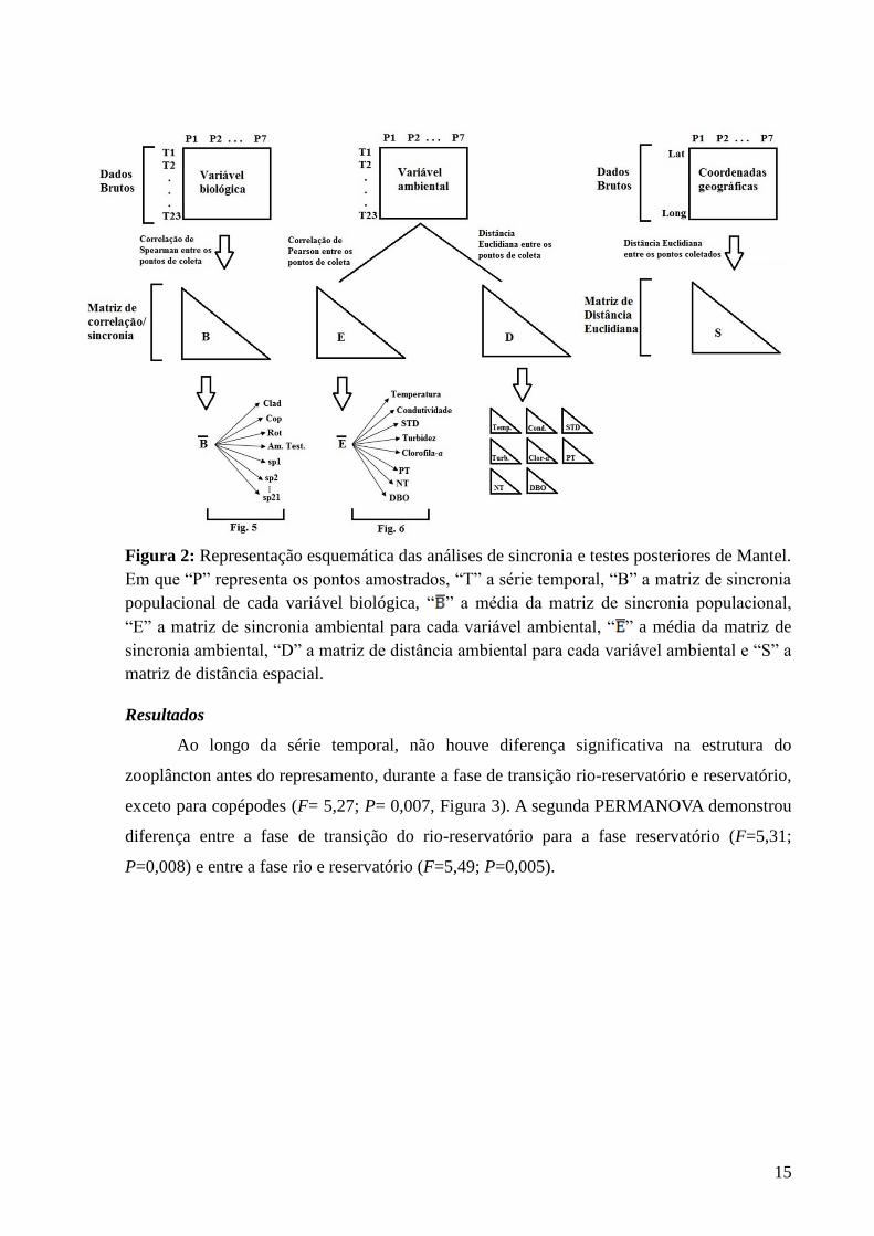
Figura 2: Representação esquemática das análises de sincronia e testes posteriores de Mantel.
Em que “P” representa os pontos amostrados, “T” a série temporal, “B” a matriz de sincronia
populacional de cada variável biológica, “ ” a média da matriz de sincronia populacional,
“E” a matriz de sincronia ambiental para cada variável ambiental, “ ” a média da matriz de
sincronia ambiental, “D” a matriz de distância ambiental para cada variável ambiental e “S” a
matriz de distância espacial.
Resultados
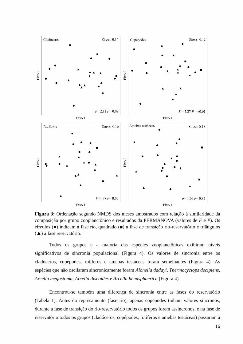
Ao longo da série temporal, não houve diferença significativa na estrutura do
zooplâncton antes do represamento, durante a fase de transição rio-reservatório e reservatório,
exceto para copépodes (F= 5,27; P= 0,007, Figura 3). A segunda PERMANOVA demonstrou
diferença entre a fase de transição do rio-reservatório para a fase reservatório (F=5,31;
P=0,008) e entre a fase rio e reservatório (F=5,49; P=0,005).
16
Figura 3: Ordenação segundo NMDS dos meses amostrados com relação à similaridade da
composição por grupo zooplanctônico e resultados da PERMANOVA (valores de F e P). Os
círculos (●) indicam a fase rio, quadrado (■) a fase de transição rio-reservatório e triângulos
(▲) a fase reservatório.
Todos os grupos e a maioria das espécies zooplanctônicas exibiram níveis
significativos de sincronia populacional (Figura 4). Os valores de sincronia entre os
cladóceros, copépodes, rotíferos e amebas testáceas foram semelhantes (Figura 4). As
espécies que não oscilaram sincronicamente foram Alonella dadayi, Thermocyclops decipiens,
Arcella megastoma, Arcella discoides e Arcella hemisphaerica (Figura 4).
Encontrou-se também uma diferença de sincronia entre as fases do reservatório
(Tabela 1). Antes do represamento (fase rio), apenas copépodes tinham valores síncronos,
durante a fase de transição do rio-reservatório todos os grupos foram assíncronos, e na fase de
reservatório todos os grupos (cladóceros, copépodes, rotíferos e amebas testáceas) passaram a

17
ser síncronos.
Figura 4: Valores médios de sincronia (± IC) do grupos e espécies comuns de zooplâncton do
reservatório Santo Antônio do Jari. Quadrados abertos: P > 0,05. Quadrados fechados: P ≤
0,05.
Tabela 1: Comparação entre a média da sincronia populacional entre toda série temporal, na
fase rio, transição rio-reservatório e reservatório, baseado em correlação de Spearman.
Valores em negrito correspondem a correlações significativas (P ≤ 0,05).
Grupos
Toda série
temporal (ver
Fig. 5) Rio
Transição rio-
reservatório Reservatório
r P r P r P r P
Cladóceros 0,31 <0,001 0,21 0.09 0,54 0,01 0,15 0,02
Copépodes 0,32 <0,001 0,25 0.05 -0,19 1 0,22 <0,001
Rotíferos 0,38 <0,001 0,21 0.09 0,07 0,25 0,19 0,01
Amebas
testáceas 0,35 <0,001 0,26 0.06 0,33 0,04 0,30 0,001
As variáveis ambientais limnológicas também apresentaram sincronias altas e
significativas (todas maiores que 0,6) (Figura 5). Além disso, a sincronia permaneceu
significativa entre as três fases do reservatório: rio, transição rio-reservatório e reservatório,
com exceção em temperatura e clorofila-a durante o enchimento do reservatório, ou seja, fase
de transição rio-reservatório (Tabela 2).

18
Figura 5: Valores médios de sincronia (± IC) das variáveis ambientais limnológicas no
reservatório Santo Antônio do Jari. Quadrados fechados: P ≤ 0,001.
Tabela 2: Comparação entre a sincronia ambiental média entre toda série temporal, na fase
rio, transição rio-reservatório e reservatório, baseado em correlação de Pearson. Valores em
negrito correspondem a correlações significativas (P ≤ 0,05).
Toda série
temporal (ver Fig.
6) Rio
Transição rio-
reservatório Reservatório
Grupos r P r P r P r P
Temperatura 0,98 <0,001 0,92 <0,001 -0,11 0,70 0,91 <0,001
Condutividade 0,83 <0,001 0,99 <0,001 0,54 0,008 0,73 <0,001
STD 0,94 <0,001 0,99 <0,001 0,81 <0,001 0,82 <0,001
Turbidez 0,68 <0,001 0,63 <0,001 0,47 0,01 0,49 <0,001
Clor-a 0,76 <0,001 0,40 <0,001 0,24 0,08 0,39 <0,002
PT 0,79 <0,001 0,77 <0,001 0,94 <0,001 0,58 <0,001
NT 0,68 <0,001 0,59 <0,001 0,75 <0,001 0,53 <0,001
DBO 0,68 <0,001 0,49 <0,001 0,88 <0,001 0,36 <0,001
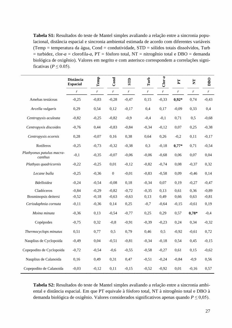
Os resultados do teste de Mantel indicam que a distância espacial entre as unidades de
amostragem não apresenta relação com as sincronias populacionais (cladóceros, copépodes,
rotíferos, amebas testáceas, 17 espécies zooplanctônicas e quatro entidades taxonômicas,
Tabela S1). Com exceção das relações existentes entre fósforo total com rotíferos (r=0,77;
P=0,01), fósforo total com amebas testáceas (r=0,92; P=0,001) e nitrogênio total com Moina
minuta (r=0,78; P=0,01), nenhuma das demais variáveis ambientais limnológicas
19
apresentaram relação com as sincronias populacionais (Tabela S1). Por fim, a distância
espacial não apresenta relação com a sincronia ambiental (Tabela S2).
Discussão
Sincronia
A sincronia populacional e ambiental é considerada um padrão ubíquo (Xu et al. 2009;
Cavanaugh et al. 2013; Seebens et al. 2013), não sendo diferente com os nossos resultados.
Os valores de sincronia populacional entre cladóceros, copépodes, rotíferos e amebas
testáceas encontrados em nosso estudo, que variaram entre 0,31 e 0,38, podem ser
considerados de magnitude intermediária, se comparados a outros trabalhos realizados em
reservatórios hidrelétricos. Por exemplo, Lansac-Tôha et al. (2008) encontrou valores entre
0,01 e 0,23 e Lodi et al. (2014), encontrou valores entre 0,54 e 0,70. Em relação à sincronia
ambiental, nossos resultados revelam valores altos para todas variáveis ambientais
limnológicas, sugerindo que o padrão espacial é similar ambientalmente ao longo do tempo. A
sincronia ambiental para clorofila-a, temperatura e condutividade foi maior do que registrado
em outros trabalhos (Magnuson et al. 1990, George et al. 2000, Järvinen et al. 2002, Xu et al.
2009, Palmer et al. 2014). Já para o nitrogênio e fósforo tivemos resultados semelhantes aos
de George et al. (2000) e maiores do que os de Huttunen et al. (2015).
Ao dividir a sincronia populacional nas três fases da construção do reservatório (rio,
transição rio-reservatório e reservatório), os nossos resultados corroboraram com nossas
hipóteses. Antes da construção da barragem (fase rio) tínhamos uma assincronia populacional
e posteriormente à formação do reservatório (fase reservatório), houve sincronia. Neste caso,
o surgimento de um padrão sincrônico pode aumentar a probabilidade de extinção local
(Heino et al. 1997, Liebhold et al. 2004).
Essa diferença de efeito sincrônico antes e depois da construção do reservatório pode
indicar que mudanças estruturais ocorreram na comunidade (Buttay et al. 2017). Porém, nosso
resultado indicou apenas mudanças estruturais para o grupo de copépodes entre a fase de
reservatório e as outras duas (fase rio e fase transição rio-reservatório). Essa falta de mudança
estrutural nos outros três grupos zooplanctônicos (cladóceros, rotíferos e amebas testáceas)
pode ser explicada porque o reservatório em estudo é considerado do tipo fio d’água, ou seja,
além de ser encaixado geologicamente, o tempo de residência da água é baixo (em nosso caso
1,5 dia). O baixo tempo de residência é mantido propositalmente para manter intacta a
Cachoeira de Santo Antônio, um ponto turístico na região, que fica a jusante da barragem.

20
Além disso, a Usina Hidrelétrica do Santo Antônio do Jari é uma usina-plataforma, ou seja,
causa um pequeno impacto no ambiente (http://www.eletrobras.com).
Mecanismos
Ao fazer a sincronia ambiental nas três fases de construção do reservatório, houve
resultados positivos na fase rio e reservatório, inferindo que os fatores extrínsecos, como o
clima e precipitação estariam atuando nas variáveis ambientais limnológicas e que o local
estudado ficou instável durante a transição do rio para o reservatório, ou seja, assíncrono
durante a transição lótica para lêntica. Isso pode ser explicado porque antes do represamento
as correntes de água e fluxo do rio eram estáveis, e depois da construção ele volta a ficar
estável, mesmo quando há toda mudança estrutural dos componentes químicos, físicos e para
alguns grupos biológicos.
Quando os valores de sincronia são baixos, demostra que fatores intrínsecos (e.g.
dispersão e variáveis ambientais limnológicas) podem estar atuando sobre as variáveis
respostas (Rusak et al. 1999, Liebhold et al. 2004, Lansac-Tôha et al. 2008) e quando os
valores de sincronia são altos, demonstra que fatores extrínsecos (e.g. clima e precipitação)
podem estar influenciando na sincronização (Kratz et al. 1987). Seguindo essa lógica e de
acordo com os nossos resultados de sincronia em toda série temporal, provavelmente fatores
intrínsecos estão atuando nas populações de zooplâncton (média do r de 0,36), ou até mesmo
por causa das características de variáveis biológicas que possuem grandes quantidades de
zeros, enquanto que fatores extrínsecos estão sincronizando as variáveis ambientais
limnológicas (média do r de 0,81), principalmente porque a sincronia ambiental não esteve
relacionada com a distância espacial.
Ao testar quais os fatores intrínsecos poderiam estar atuando na sincronia
populacional, apenas algumas variáveis ambientais limnológicas, principalmente aquelas
relacionadas a concentração de nutrientes, foram correlacionadas com a sincronia de algumas
espécies e grupos zooplanctônicos. Sabe-se que os nutrientes possuem uma relação positiva
com a riqueza e abundância do zooplâncton (Bozelli et al. 2015). O fósforo, por exemplo,
correlacionou-se com as amebas testáceas e com os rotíferos. Os rotíferos já são conhecidos
por serem oportunistas e se desenvolverem bem em reservatórios pré-formados (Descloux and
Cottet 2016), pois durante a implementação da barragem há entrada de nutrientes terrestres e
troncos de árvores (Emery et al. 2015). Da mesma forma, a sincronia da Moina minuta
(cladócero) correlacionou-se com concentrações de nitrogênio, e estudos anteriores mostram
que essa espécie tem sua abundância correlacionada com nutrientes (Vieira et al. 2011).

21
Assim, apenas algumas variáveis ambientais de nutrientes atuaram na sincronia populacional,
demonstrando que pode haver alguma outra variável ambiental local sincronizando a
população, como o pH, a profundidade do ponto de coleta, velocidade da água, tempo de
residência da água do reservatório no dia da coleta ou até mesmo a interação trófica entre as
populações e comunidades. Outros autores já encontraram essas variáveis relacionadas com a
abundância de zooplâncton (Bowman et al. 2014, Silva et al. 2014, Simões et al. 2015).
Já a distância espacial não foi correlacionada com nenhuma das sincronias, refutando
nossa hipótese de que em distâncias menores teríamos valores de sincronia maiores. Isso pode
ser influenciado por um efeito de escala, no qual a distância entre os pontos são muito
pequenas (< 15 km), e, geralmente, padrões sincrônicos são encontrados em distâncias
maiores do que 100 km (Hanski and Woiwod 1993, Defriez et al. 2016).
Aplicações para o monitoramento ambiental
Nosso resultado mostra que a sincronia espacial é onipresente, sendo portanto muito
difícil avaliar completamente quais são os fatores que a influenciam. Essa dificuldade também
é encontrada por outros autores (Gouhier et al. 2010, Cavanaugh et al. 2013, Seebens et al.
2013), isso porque todos mecanismos podem produzir respostas quase idênticas de sincronia
entre as populações (Liebhold et al. 2004). Entretanto, independente dos mecanismos atuantes
na sincronia, o fato de saber se as populaçoes são síncronas ou assíncronas tem aplicações em
programas de monitoramento (Lansac-Tôha et al. 2008), gestão de conservação de espécies e
surtos de pragas (Liebhold et al. 2004). Para a região desse estudo, sugere-se um aumento de
pontos amostrais dentro do reservatório uma vez que a sincronia populacional foi baixa. Por
outro lado, em relação à elevada sincronia ambiental, uma estratégia possível para otimizar o
monitoramento seria a redução dos pontos de coleta. Pois o ideal é aumentar a amostragem
quando a sincronia é muito baixa e diminuir quando alta, já que poucos pontos amostrados
seriam suficientes para responder toda área (Takahashi et al. 2008). Assim, os recursos
financeiros e pessoais, podem ser distribuídos de uma melhor forma ao aperfeiçoar o
gerenciamento da represa.
Conclusão
A sincronia populacional foi baixa e pode ser atribuída a algumas variáveis ambientais
limnológicas, já a sincronia ambiental foi alta e o motivo pode estar ligado a fatores
extrínsecos (ex. precipitação e temperatura do ar). Tanto a sincronia populacional quanto a
ambiental não foram relacionadas pela distância espacial. Ao analisar a sincronia nas três
fases do reservatório (rio, transição rio-reservatório e reservatório), concluímos que antes da
22
construção do reservatório tínhamos uma assincronia populacional, e com a implementação
da barragem, houve a sincronia. A sincronia ambiental existia na fase rio e reservatório, porém
o ambiente ficou assíncrono durante a transição lótica para lêntica. Assim, a sincronia é
visível em nossos resultados, porém os mecanismos que estão atuando ainda não são claros,
indicando que mais de um fator pode estar influenciando na dinâmica. Para melhor
compreensão dos mecanismos atuantes na dinâmica populacional e ambiental, sugerimos que
além de usar as variáveis ambientais limnológicas e fazer a sincronia espacial, deve-se usar
dados meteorológicos e de paisagem que são considerados fatores extrínsecos.
Referências
Anneville, O., S. Souissi, S. Gammeter, and D. Straile. 2004. Seasonal and inter-annual scales
of variability in phytoplankton assemblages: Comparison of phytoplankton dynamics in
three peri-alpine lakes over a period of 28 years. Freshwater Biology 49:98–115.
Arnott, S. E., B. Keller, P. J. Dillon, N. Yan, M. Paterson, and D. Findlay. 2003. Using
Temporal Coherence to Determine the Response to Climate Change in Boreal Shield
Lakes. Environmental Monitoring and Assessment 88:365–388.
Baines, S. B., K. E. Webster, T. K. Kratz, S. R. Carpenter, and J. J. Magnuson. 2000.
Synchronous behavior of temperature, calcium, and chlorophyll in lakes of Northern
Wisconsin. Ecology 81:815–825.
Baxter, R. M. 1977. Environmental Effects of Dams and Impoundments. Annual Review of
Ecology and Systematics 8:255–283.
Bjørnstad, O. N., R. A. Ims, and X. Lambin. 1999. Spatial population dynamics: analyzing
patterns and processes of population synchrony. Trends in ecology & evolution 14:427–
432.
Bonecker, C. C., N. R. Simões, C. V. Minte-Vera, F. A. Lansac-Tôha, L. F. M. Velho, and Â.
A. Agostinho. 2013. Temporal changes in zooplankton species diversity in response to
environmental changes in an alluvial valley. Limnologica - Ecology and Management of
Inland Waters 43:114–121.
Bottrell, H. H., A. Ducan, Z. M. Gliwicz, E. Grygierek, A. Herzig, A. Hillbricht-Ilkowska, H.
Kurasawa, P. Larsson, and T. Weglenska. 1976. Review of some problems in
zooplankton production studies. Norwegian Journal of Zoology 24:419–456.
Bowman, M. F., C. Nussbaumer, and N. M. Burgess. 2014. Community composition of lake
zooplankton, benthic macroinvertebrates and forage fish across a pH gradient in
Kejimkujik National Park, Nova Scotia, Canada. Water, Air, and Soil Pollution 225.

23
Bozelli, R. L., S. M. Thomaz, A. A. Padial, P. M. Lopes, and L. M. Bini. 2015. Floods
decrease zooplankton beta diversity and environmental heterogeneity in an Amazonian
floodplain system. Hydrobiologia 753:233–241.
Buttay, L., B. Cazelles, A. Miranda, G. Casas, E. Nogueira, and R. González-Quirós. 2017.
Environmental multi-scale effects on zooplankton inter-specific synchrony. Limnology
and Oceanography.
Cattadori, I. M., S. Merler, and P. J. Hudson. 2000. Searching for mechanisms of synchrony in
spatially structured gamebird populations. Journal of Animal Ecology 69:620–638.
Cavanaugh, K. C., B. E. Kendall, D. A. Siegel, D. C. Reed, F. Alberto, and J. Assis. 2013.
Synchrony in dynamics of giant kelp forests is driven by both local recruitment and
regional environmental controls. Ecology 94:499–509.
Defriez, E. J., L. W. Sheppard, P. C. Reid, and D. C. Reuman. 2016. Climate change-related
regime shifts have altered spatial synchrony of plankton dynamics in the North Sea.
Global Change Biology 22:2069–2080.
Descamps, S., H. Strøm, and H. Steen. 2013. Decline of an arctic top predator: Synchrony in
colony size fluctuations, risk of extinction and the subpolar gyre. Oecologia 173:1271–
1282.
Descloux, S., and M. Cottet. 2016. 5 years of monitoring of zooplankton community
dynamics in a newly impounded sub-tropical reservoir in Southeast Asia (Nam Theun 2,
Lao PDR). Hydroécologie Appliquée 19:197–216.
Downing, A. L., B. L. Brown, E. M. Perrin, T. H. Keitt, and M. A. Leibold. 2008.
Environmental Fluctuations Induce Scale-dependent Compensation and Increase
Stability in Plankton Ecosystems. Ecology 89:3204–3214.
Emery, K. A., G. M. Wilkinson, F. G. Ballard, and M. L. Pace. 2015. Use of allochthonous
resources by zooplankton in reservoirs. Hydrobiologia 758:257–269.
Filizola, N., J. L. Guyot, M. Molinier, V. Guimarães, E. Oliveira, and M. A. Freitas. 2002.
Caracterização hidrológica da Bacia Amazônica. Pages 33–53in A. C. E. Rivas and de
C. Freitas, editors.Amazônia uma perspectiva interdisciplinar. EDUA, Manaus.
George, D. G., J. F. Talling, and E. Rigg. 2000. Factors influencing the temporal coherence of
five lakes in the English Lake District. Freshwater Biology 43:449–461.
Golterman, H. L., R. S. Clymo, and M. A. M. Ohnstad. 1978. Methods for Physical and
Chemical Analysis of Fresh Waters. Blackwell Scientific, Oxford.
Gouhier, T. C., and F. Guichard. 2014. Synchrony: quantifying variability in space and time.
Methods in Ecology and Evolution 5:524–533.

24
Gouhier, T. C., F. Guichard, and B. A. Menge. 2010. Ecological processes can synchronize
marine population dynamics over continental scales. Proceedings of the National
Academy of Sciences of the United States of America 107:8281–6.
Hanski, I., and I. P. Woiwod. 1993. Spatial synchrony in the dynamics of moth and aphid
populations. Journal of Animal Ecology 62:656–668.
Havel, J. E., and J. B. Shurin. 2004. Mechanisms, effects, and scales of dispersal in freshwater
zooplankton. Limnology and Oceanography 49:1229–1238.
Heino, M., V. Kaitala, E. Ranta, and J. Lindström. 1997. Synchronous dynamics and rates of
extinction in spatially structured populations. Proceedings of the Royal Society of
London B: Biological Sciences 264:481–486.
Huttunen, K. L., H. Mykrä, A. Huusko, A. Mäki-Petäys, T. Vehanen, T. Muotka, A. J. Allstadt,
A. M. Liebhold, D. M. Johnson, R. E. Davis, and K. J. Haynes. 2015. Testing for
temporal coherence across spatial extents: The roles of climate and local factors in
regulating stream macroinvertebrate community dynamics. Ecology 96:2935–2946.
Ims, R. A., and H. Steen. 1990. Geographical Synchrony in Microtine Population Cycles: A
Theoretical Evaluation of the Role of Nomadic Avian Predators. Oikos 57:381.
Järvinen, M., M. Rask, J. Ruuhijärvi, and L. Arvola. 2002. Temporal coherence in water
temperature and chemistry under the ice of boreal lakes (Finland). Water Research
36:3949–3956.
Jiao, Y., R. O. Reilly, E. Smith, and D. Orth. 2016. Bayesian statistical catch-at-age approach.
Journal of Marine Science 73:1725–1738.
Kendall, B. E., O. N. Bjørnstad, J. Bascompte, T. H. Keitt, and W. F. Fagan. 2000. Dispersal,
environmental correlation, and spatial synchrony in population dynamics. American
Naturalist 155:628–636.
Koenig, W. D. 1999. Spatial autocorrelation of ecological phenomena. Trends in Ecology and
Evolution 14:22–26.
Kratz, T. K., T. M. Frost, and J. J. Magnuson. 1987. Inferences from Spatial and Temporal
Variability in Ecosystems: Long-Term Zooplankton Data from Lakes. The American
Naturalist 129:830–846.
Lansac-Tôha, F. A., L. M. Bini, L. F. M. Velho, C. C. Bonecker, E. M. Takahashi, and L. C. G.
Vieira. 2008. Temporal coherence of zooplankton abundance in a tropical reservoir.
Hydrobiologia 614:387–399.
Liebhold, A., W. D. Koenig, and O. N. Bjornstad. 2004. Spatial Synchrony in Population
Dynamics. Annual Review of Ecology, Evolution and Systematics 35:467–490.

25
Lodi, S., L. F. M. Velho, P. Carvalho, and L. M. Bini. 2014. Patterns of zooplankton
population synchrony in a tropical reservoir. Journal of Plankton Research 36:966–977.
Mackereth, F. J. H., J. Heron, and J. F. Talling. 1978. Water Analysis: Some Revised Methods
for Limnologists. Freshwater Biological Association.
Magnuson, J. J., B. J. Benson, and T. K. Kratz. 1990. Temporal coherence in the limonology
of a suite of lakes in Wisconsin, U.S.A. Freshwater Biology 23:145–149.
Oksanen, J., F. Blanchet, Guillaume, M. Friendly, R. Kindt, P. Legendre, D. Mcglinn, P. R.
Minchin, R. B. O ’hara, G. L. Simpson, P. Solymos, H. Stevens, E. Szoecs, and H.
Wagner. 2016. Vegan: Community Ecology Package. R package version 2.4-0.
Ostfeld, R. S., and F. Keesing. 2000. Pulsed resources and community dynamics of consumers
in terrestrial ecosystems. Trends in Ecology & Evolution 15:232–237.
Palmer, M. E., N. D. Yan, and K. M. Somers. 2014. Climate change drives coherent trends in
physics and oxygen content in North American lakes. Climatic Change 124:285–299.
R Development Core Team. 2017. R: A language and environment for statistical computing. R
Foundation for Statistical Computing, Vienna, Austria.
Rhodes, J. R., and N. Jonz??n. 2011. Monitoring temporal trends in spatially structured
populations: how should sampling effort be allocated between space and time?
Ecography 34:1040–1048.
Roche, E. A., T. L. Shaffer, C. M. Dovichin, M. H. Sherfy, M. J. Anteau, and M. T.
Wiltermuth. 2016. Synchrony of Piping Plover breeding populations in the U.S. Northern
Great Plains. The Condor: Ornithological Applications 118:558–570.
Rusak, J. A., N. D. Yan, K. M. Somers, and D. J. McQueen. 1999. The Temporal Coherence
of Zooplankton Population Abundances in Neighboring North‐Temperate Lakes. The
American Naturalist 153:46–58.
Seebens, H., U. Einsle, and D. Straile. 2013. Deviations from synchrony: Spatio-temporal
variability of zooplankton community dynamics in a large lake. Journal of Plankton
Research 35:22–32.
Silva, L. H. S., V. L. M. Huszar, M. M. Marinho, L. M. Rangel, J. Brasil, C. D. Domingues,
C. C. Branco, and F. Roland. 2014. Drivers of phytoplankton, bacterioplankton, and
zooplankton carbon biomass in tropical hydroelectric reservoirs. Limnologica 48:1–10.
Simões, N. R., A. H. Nunes, J. D. Dias, F. A. Lansac-Tôha, L. F. M. Velho, and C. C.
Bonecker. 2015. Impact of reservoirs on zooplankton diversity and implications for the
conservation of natural aquatic environments. Hydrobiologia 758:3–17.

26
Soininen, J., M. Kokocinski, S. Estlander, J. Kotanen, and J. Heino. 2007. Neutrality, niches,
and determinants of plankton metacommunity structure across boreal wetland ponds.
Ecoscience 14:146–154.
Stanford, J. A., and J. V. Ward. 2001. Revisiting the serial discontinuity concept. Regulated
Rivers: Research & Management 17:303–310.
Stange, E. E., M. P. Ayres, and J. A. Bess. 2011. Concordant population dynamics of
Lepidoptera herbivores in a forest ecosystem. Ecography 34:772–779.
Takahashi, E. M., F. A. Lansac-Tôha, L. F. M. Velho, and L. M. Bini. 2008. The temporal
asynchrony of planktonic cladocerans population at different environments of the upper
Paraná River floodplain. International Review of Hydrobiology 93:679–689.
Tedesco, P. A., B. Hugueny, D. Paugy, and Y. Fermon. 2004. Spatial synchrony in population
dynamics of West African fishes: A demonstration of an intraspecific and interspecific
Moran effect. Journal of Animal Ecology 73:693–705.
Vieira, A. C. B., A. M. A. Medeiros, L. L. Ribeiro, and M. C. Crispim. 2011. Dinâmica
populacional de moina minuta hansen (1899), ceriodaphnia cornuta sars (1886) e
diaphanosoma spinulosum herbst (1967) (crustacea: Branchiopoda) em diferentes faixas
de concentração de nutrientes (N e P). Acta Limnologica Brasiliensia 23:48–56.
Wetzel, R. G., and G. E. Likens. 2000. Special Lake Types. Pages 355–360Limnological
Analyses. Springer New York, New York, NY.
Wu, N., T. Tang, X. Fu, W. Jiang, F. Li, S. Zhou, Q. Cai, and N. Fohrer. 2009. Impacts of
cascade run-of-river dams on benthic diatoms in the Xiangxi River, China. Aquatic
Sciences 72:117–125.
Xu, Y., Q. Cai, M. Shao, and X. Han. 2012. Patterns of asynchrony for phytoplankton
fluctuations from reservoir mainstream to a tributary bay in a giant dendritic reservoir
(Three Gorges Reservoir, China). Aquatic Sciences 74:287–300.
Xu, Y. Y., L. Wang, Q. H. Cai, and L. Ye. 2009. Temporal coherence of chlorophyll a during a
spring phytoplankton bloom in Xiangxi bay of three-gorges reservoir, China.
International Review of Hydrobiology 94:656–672.
Zhao, K., K. Song, Y. Pan, L. Wang, L. Da, and Q. Wang. 2017. Metacommunity structure of
zooplankton in river networks: Roles of environmental and spatial factors. Ecological
Indicators 73:96–104.
MATERIAL SUPLEMENTAR (I)
27
Tabela S1: Resultados do teste de Mantel simples avaliando a relação entre a sincronia popu-
lacional, distância espacial e sincronia ambiental estimada de acordo com diferentes variáveis
(Temp = temperatura da água, Cond = condutividade, STD = sólidos totais dissolvidos, Turb
= turbidez, clor-a = clorofila-a, PT = fósforo total, NT = nitrogênio total e DBO = demanda
biológica de oxigênio). Valores em negrito e com asterisco correspondem a correlações signi-
ficativas (P ≤ 0.05).
Distância
Espacial Tem
p
Co
nd
ST
D
Tu
rb
Clo
r-a
PT
NT
DB
O
r
r
r
r
r
r
r
r
r
Amebas testáceas -0,25
-0,83
-0,28
-0,47
0,15
-0,33
0,92*
0,74
-0,43
Arcella vulgaris 0,29
0,54
0,12
-0,17
0,4
0,17
-0,09
0,33
0,4
Centropyxis aculeata -0,82
-0,25
-0,82
-0,9
-0,4
-0,1
0,71
0,5
-0,68
Centropyxis discoides -0,76
0,44
-0,83
-0,84
-0,34
-0,12
0,07
0,25
-0,38
Centropyxis ecornis 0,28
-0,07
0,16
0,38
0,64
0,26
-0,2
0,11
-0,17
Rotíferos -0,25
-0,73
-0,32
-0,38
0,3
-0,18
0,77*
0,71
-0,54
Plathyonus patulus macra-
canthus -0,1
-0,35
-0,07
-0,06
-0,06
-0,68
0,06
0,07
0,04
Plathyas quadricornis -0,22
-0,25
0,01
-0,12
-0,82
-0,74
0,08
-0,37
0,32
Lecane bulla -0,25
-0,36
0
-0,01
-0,83
-0,58
0,09
-0,46
0,14
Bdelloidea -0,24
-0,54
-0,08
0,18
-0,34
0,07
0,19
-0,27
-0,47
Cladóceros -0,84
-0,29
-0,82
-0,72
-0,35
0,13
0,61
0,36
-0,89
Bosminopsis deitersi -0,52
-0,18
-0,63
-0,63
0,13
0,49
0,66
0,63
-0,81
Ceriodaphnia cornuta -0,11
-0,36
0,14
0,25
-0,7
-0,64
-0,15
-0,61
0,19
Moina minuta -0,36
0,13
-0,54
-0,77
0,25
0,29
0,57
0,78*
-0,4
Copépodes -0,75
0,32
-0,8
-0,91
-0,39
-0,23
0,24
0,34
-0,32
Thermocyclops minutus 0,51
0,77
0,5
0,79
0,46
0,5
-0,92
-0,61
0,72
Nauplius de Cyclopoida -0,49
0,04
-0,51
-0,81
-0,34
-0,18
0,54
0,45
-0,15
Copepodito de Cyclopoida -0,72
-0,54
-0,6
-0,55
-0,58
-0,27
0,61
0,15
-0,62
Nauplius de Calanoida 0,16
0,49
0,31
0,47
-0,51
-0,24
-0,84
-0,9
0,56
Copepodito de Calanoida -0,03 -0,12 0,11 -0,15 -0,52 -0,92 0,01 -0,16 0,57
Tabela S2: Resultados do teste de Mantel simples avaliando a relação entre a sincronia ambi-
ental e distância espacial. Em que PT equivale à fósforo total, NT à nitrogênio total e DBO à
demanda biológica de oxigênio. Valores considerados significativos apenas quando P ≤ 0,05).

28
Distância espacial
r P
Temperatura 0,13 0,63
Condutividade -0,93 0,97
STD -0,88 0,92
Turbidez -0,50 0,94
Clorofila-a -0,66 0,79
PT -0,16 0,72
NT -0,08 0,52
DBO -0,81 0,95
Tabela S3: Valores médios, mínimos (Min), máximos (Max) e desvio padrão (DP) das variá-
veis ambientais limnológicas.
Variáveis Média Min-Max DP
Temperatura 28,06 18 - 33,3 3,63
Condutividade 28,79 7 - 101 15,99
STD 14,96 4 - 51 7,59
Turbidez 8,9 1,03 - 25,2 5,63
Clorofila-a 4,45 0 - 86,01 9,9
PT 0,02 0 - 0,21 0,02
NT 0,87 0 - 0,32 0,49
DBO 1,87 0,1 - 6 1,34

29
CAPÍTULO II
Manuscrito aceito para publicação na Ecological Indicators.
(https://www.journals.elsevier.com/ecological-indicators)
Biodiversity shortcuts in biomonitoring of novel ecosystems
Abstract
Hydropower reservoirs are novel ecosystems that present different challenges for the design
of biomonitoring programs. To ensure long-term programs and wide spatial coverage, it is
important to test the reliability of different cost-saving strategies that have been widely
evaluated among researchers, such as taxonomic suffi- ciency, numerical sufficiency and
surrogate groups. Using data on zooplankton composition, our objective was to test whether
these strategies could be applied to increase the efficiency of biomonitoring programs in
reservoirs. Zooplankton data were collected at the Santo Antônio do Jari Hydroelectric Plant,
which is located between the states of Pará and Amapá (Amazon region, Brazil), over 23
months between 2012 and 2015. The data were organized in different taxonomic groups
(cladocerans, copepods, rotifers and testate amoebae) and matrices by decreasing the
taxonomic resolution (from species to genera and families) and the numerical resolution (from
species abundance to species presence/absence) of the data. The ordination patterns obtained
with Principal Coordinate Analysis for the different matrices were compared using Procrustes
analyses. Our results suggest that ordination patterns using genus-level data were similar to
those obtained with species-level data. However, analyses based on family-level data were
often unable to reproduce results based on species-level data. Ordination patterns using
presence/absence data were similar to those obtained from abundance data. We also found that
the strengths of the relationships between ordinations derived from different taxonomic
groups (e.g., rotifers and cladocerans) were low and often not significant. We conclude that
the use of zooplankton genera and presence/absence data may be a reliable strategy to monitor
reservoirs. However, our results highlight the need to monitor different zooplankton groups,
as the ordination patterns depicted by a given group were poorly related to those generated by
a second zooplankton group.
Keywords: Jari River, Amazon; reservoir; cross-taxon congruence; taxonomic resolution;
taxonomic sufficiency; numerical resolution.
1. Introduction
River regulation by dams is an important driver of biodiversity loss in freshwater
systems (Dudgeon et al., 2006). The change in hydrology caused by impoundments triggers
several other changes in water quality, ecosystem processes and structure of aquatic
communities. For instance, one can anticipate the creation of reservoir zones with different
limnological characteristics (Kimmel et al., 1990) and periods with water stratification,
mainly close to the dam (i.e., in the lacustrine zone), that were negligible or completely absent
before damming. In terms of ecosystem processes, an increase in the primary productivity rate
30
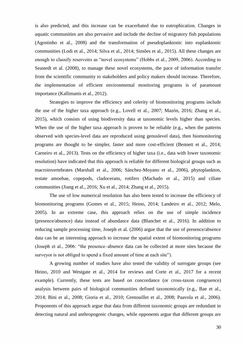
is also predicted, and this increase can be exacerbated due to eutrophication. Changes in
aquatic communities are also pervasive and include the decline of migratory fish populations
(Agostinho et al., 2008) and the transformation of pseudoplanktonic into euplanktonic
communities (Lodi et al., 2014; Silva et al., 2014; Simões et al., 2015). All these changes are
enough to classify reservoirs as “novel ecosystems” (Hobbs et al., 2009, 2006). According to
Seastedt et al. (2008), to manage these novel ecosystems, the pace of information transfer
from the scientific community to stakeholders and policy makers should increase. Therefore,
the implementation of efficient environmental monitoring programs is of paramount
importance (Kallimanis et al., 2012).
Strategies to improve the efficiency and celerity of biomonitoring programs include
the use of the higher taxa approach (e.g., Lovell et al., 2007; Mazón, 2016; Zhang et al.,
2015), which consists of using biodiversity data at taxonomic levels higher than species.
When the use of the higher taxa approach is proven to be reliable (e.g., when the patterns
observed with species-level data are reproduced using genuslevel data), then biomonitoring
programs are thought to be simpler, faster and more cost-efficient (Bennett et al., 2014;
Carneiro et al., 2013). Tests on the efficiency of higher taxa (i.e., data with lower taxonomic
resolution) have indicated that this approach is reliable for different biological groups such as
macroinvertebrates (Marshall et al., 2006; Sánchez-Moyano et al., 2006), phytoplankton,
testate amoebae, copepods, cladocerans, rotifers (Machado et al., 2015) and ciliate
communities (Jiang et al., 2016; Xu et al., 2014; Zhang et al., 2015).
The use of low numerical resolution has also been tested to increase the efficiency of
biomonitoring programs (Gomes et al., 2015; Heino, 2014; Landeiro et al., 2012; Melo,
2005). In an extreme case, this approach relies on the use of simple incidence
(presence/absence) data instead of abundance data (Blanchet et al., 2016). In addition to
reducing sample processing time, Joseph et al. (2006) argue that the use of presence/absence
data can be an interesting approach to increase the spatial extent of biomonitoring programs
(Joseph et al., 2006: “the presence–absence data can be collected at more sites because the
surveyor is not obliged to spend a fixed amount of time at each site”).
A growing number of studies have also tested the validity of surrogate groups (see
Heino, 2010 and Westgate et al., 2014 for reviews and Corte et al., 2017 for a recent
example). Currently, these tests are based on concordance (or cross-taxon congruence)
analysis between pairs of biological communities defined taxonomically (e.g., Bae et al.,
2014; Bini et al., 2008; Gioria et al., 2010; Grenouillet et al., 2008; Paavola et al., 2006).
Proponents of this approach argue that data from different taxonomic groups are redundant in
detecting natural and anthropogenic changes, while opponents argue that different groups are
31
needed to detect subtle environmental changes (Bowman et al., 2008). However, it appears
that a large number of studies support the view of the “opponents” (e.g., Backus-Freer and
Pyron, 2015; Guareschi et al., 2015; Kimmel and Argent, 2016; Rosa et al., 2014; Vilmi et al.,
2016) instead of the view of “proponents” of the surrogacy approach (e.g., Kilgour and
Barton, 1999).
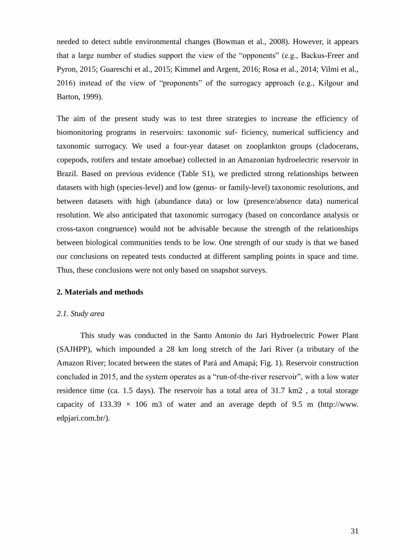
The aim of the present study was to test three strategies to increase the efficiency of
biomonitoring programs in reservoirs: taxonomic suf- ficiency, numerical sufficiency and
taxonomic surrogacy. We used a four-year dataset on zooplankton groups (cladocerans,
copepods, rotifers and testate amoebae) collected in an Amazonian hydroelectric reservoir in
Brazil. Based on previous evidence (Table S1), we predicted strong relationships between
datasets with high (species-level) and low (genus- or family-level) taxonomic resolutions, and
between datasets with high (abundance data) or low (presence/absence data) numerical
resolution. We also anticipated that taxonomic surrogacy (based on concordance analysis or
cross-taxon congruence) would not be advisable because the strength of the relationships
between biological communities tends to be low. One strength of our study is that we based
our conclusions on repeated tests conducted at different sampling points in space and time.
Thus, these conclusions were not only based on snapshot surveys.
2. Materials and methods
2.1. Study area
This study was conducted in the Santo Antonio do Jari Hydroelectric Power Plant
(SAJHPP), which impounded a 28 km long stretch of the Jari River (a tributary of the
Amazon River; located between the states of Pará and Amapá; Fig. 1). Reservoir construction
concluded in 2015, and the system operates as a “run-of-the-river reservoir”, with a low water
residence time (ca. 1.5 days). The reservoir has a total area of 31.7 km2 , a total storage
capacity of 133.39 × 10⁶ m3 of water and an average depth of 9.5 m (http://www.
edpjari.com.br/).

32
Fig. 1. Santo Antonio do Jari Hydroelectric Power Plant (South America, Brazil, Pará/ Amapá
states). The reservoir area is shown in gray. Sampling sites are represented as black circles (•).
2.2. Sampling
We conducted 23 sampling campaigns: nine before the impoundment (from February
2012 to February 2014), three during the filling period (May to July 2014) and eleven during
the operation period (August 2014 to August 2015) of the SAJHPP. The number of sampling
sites varied from 14 during the beginning of the study to 18 sites after the filling of the
reservoir. The sampling sites were distributed along the main axis of the reservoir and along
some tributaries of the Jari River.
In each sampling site, a zooplankton sample was collected at a depth of 0.5 m by
filtering 1000 L of water through a 68 µm plankton net. Samples were fixed with a 4%
solution of calcium carbonate-buffered formaldehyde. For species identification and
abundance analyses, zooplankton samples were concentrated to volumes ranging from 75 mL
to 300 mL, depending on the concentration of suspended sediment in the samples. Larger
volumes were necessary to observe specimens in samples with high suspended sediment
concentrations. Prior to analysis, the samples were stained with Rose Bengal to facilitate the
visualization of the organisms. Samples were analyzed under a microscope (Olympus CX31 –
400x) to determine zooplankton composition and abundance using Sedgwick-Rafter
chambers. Five sub-samples of 1.5 mL (7.5 mL in total) obtained with a Hensen-Stempel
pipette were analyzed, and the results were expressed as individuals per m3. Samples with
33
very low densities were analyzed entirely (Bottrell et al., 1976).
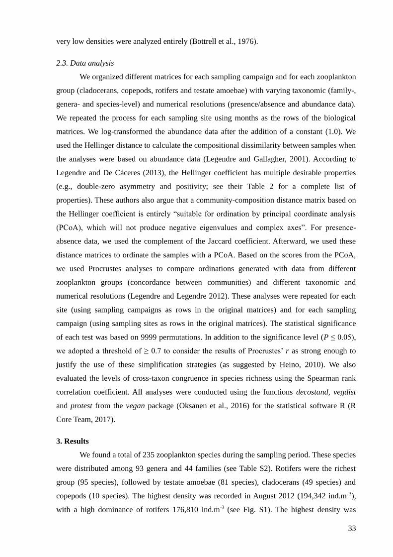
2.3. Data analysis
We organized different matrices for each sampling campaign and for each zooplankton
group (cladocerans, copepods, rotifers and testate amoebae) with varying taxonomic (family-,
genera- and species-level) and numerical resolutions (presence/absence and abundance data).
We repeated the process for each sampling site using months as the rows of the biological
matrices. We log-transformed the abundance data after the addition of a constant (1.0). We
used the Hellinger distance to calculate the compositional dissimilarity between samples when
the analyses were based on abundance data (Legendre and Gallagher, 2001). According to
Legendre and De Cáceres (2013), the Hellinger coefficient has multiple desirable properties
(e.g., double-zero asymmetry and positivity; see their Table 2 for a complete list of
properties). These authors also argue that a community-composition distance matrix based on
the Hellinger coefficient is entirely “suitable for ordination by principal coordinate analysis
(PCoA), which will not produce negative eigenvalues and complex axes”. For presence-
absence data, we used the complement of the Jaccard coefficient. Afterward, we used these
distance matrices to ordinate the samples with a PCoA. Based on the scores from the PCoA,
we used Procrustes analyses to compare ordinations generated with data from different
zooplankton groups (concordance between communities) and different taxonomic and
numerical resolutions (Legendre and Legendre 2012). These analyses were repeated for each
site (using sampling campaigns as rows in the original matrices) and for each sampling
campaign (using sampling sites as rows in the original matrices). The statistical significance
of each test was based on 9999 permutations. In addition to the significance level (P ≤ 0.05),
we adopted a threshold of ≥ 0.7 to consider the results of Procrustes’ r as strong enough to
justify the use of these simplification strategies (as suggested by Heino, 2010). We also
evaluated the levels of cross-taxon congruence in species richness using the Spearman rank
correlation coefficient. All analyses were conducted using the functions decostand, vegdist
and protest from the vegan package (Oksanen et al., 2016) for the statistical software R (R
Core Team, 2017).
3. Results
We found a total of 235 zooplankton species during the sampling period. These species
were distributed among 93 genera and 44 families (see Table S2). Rotifers were the richest
group (95 species), followed by testate amoebae (81 species), cladocerans (49 species) and
copepods (10 species). The highest density was recorded in August 2012 (194,342 ind.m-3),
with a high dominance of rotifers 176,810 ind.m-3 (see Fig. S1). The highest density was

34
recorded at the sampling site 7 (289,330 ind.m-3) (see Fig. S2). This result can be explained
by considering that this site has low water flow, favoring population growth.
In general, the relationships between the biological matrices at species and genera
levels were significant over time (Fig. 2). Similar results were obtained when the matrices
were organized for each sampling site (where the rows of the matrices were the sampling
campaigns; Fig. 3). The correlation strengths were more variable for testate amoebae and
rotifers. For testate amoebae, the correlations were more frequently non-significant.
Fig. 2. Variation in the taxonomic sufficiency strength (as measured by Procrustes’ r) for
different zooplankton groups in the Santo Antonio do Jari Reservoir. For each sampling
campaign the comparisons were made between species-level and genus-level data,
considering the sampling sites as rows in the matrices. Non-significant values (P ≥ 0.05) are
indicated by unfilled symbols.
35
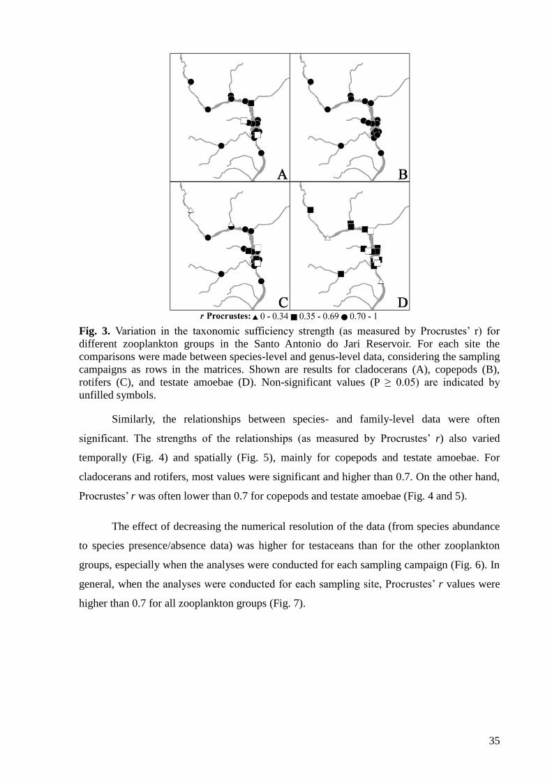
Fig. 3. Variation in the taxonomic sufficiency strength (as measured by Procrustes’ r) for
different zooplankton groups in the Santo Antonio do Jari Reservoir. For each site the
comparisons were made between species-level and genus-level data, considering the sampling
campaigns as rows in the matrices. Shown are results for cladocerans (A), copepods (B),
rotifers (C), and testate amoebae (D). Non-significant values (P ≥ 0.05) are indicated by
unfilled symbols.
Similarly, the relationships between species- and family-level data were often
significant. The strengths of the relationships (as measured by Procrustes’ r) also varied
temporally (Fig. 4) and spatially (Fig. 5), mainly for copepods and testate amoebae. For
cladocerans and rotifers, most values were significant and higher than 0.7. On the other hand,
Procrustes’ r was often lower than 0.7 for copepods and testate amoebae (Fig. 4 and 5).
The effect of decreasing the numerical resolution of the data (from species abundance
to species presence/absence data) was higher for testaceans than for the other zooplankton
groups, especially when the analyses were conducted for each sampling campaign (Fig. 6). In
general, when the analyses were conducted for each sampling site, Procrustes’ r values were
higher than 0.7 for all zooplankton groups (Fig. 7).

36
Fig. 4. Variation in the taxonomic sufficiency strength (as measured by Procrustes’ r) for
different zooplankton groups in the Santo Antonio do Jari Reservoir. For each sampling
campaign the comparisons were made between species-level and family-level data,
considering the sampling sites as rows in the matrices. Non-significant values (P ≥ 0.05) are
indicated by unfilled symbols.
Fig. 5. Variation in the taxonomic sufficiency strength (as measured by Procrustes’ r) for
different zooplankton groups in the Santo Antonio do Jari Reservoir. For each site the
comparisons were made between species-level and family-level data, considering the
sampling campaigns as rows in the matrices. Shown are results for cladocerans (A), copepods
(B), rotifers (C), and testate amoebae (D). Non-significant values (P ≥ 0.05) are indicated by
unfilled symbols.

37
Fig. 6. Variation in the numerical sufficiency strength (as measured by Procrustes’ r) for
different zooplankton groups in the Santo Antonio do Jari Reservoir. For each sampling
campaign the comparisons were made between abundance and presence/absence data,
considering the sampling sites as rows in the matrices. Non-significant values (P ≥ 0.05) are
indicated by unfilled symbols.
Fig. 7. Variation in the numerical sufficiency strength (as measured by Procrustes’ r) for
different zooplankton groups in the Santo Antonio do Jari Reservoir. For each site the
comparisons were made between abundance and presence/absence data, considering the
sampling campaigns as rows in the matrices. Shown are results for cladocerans (A), copepods
(B), rotifers (C), and testate amoebae (D). Non-significant values (P ≥ 0.05) are indicated by
unfilled symbols.
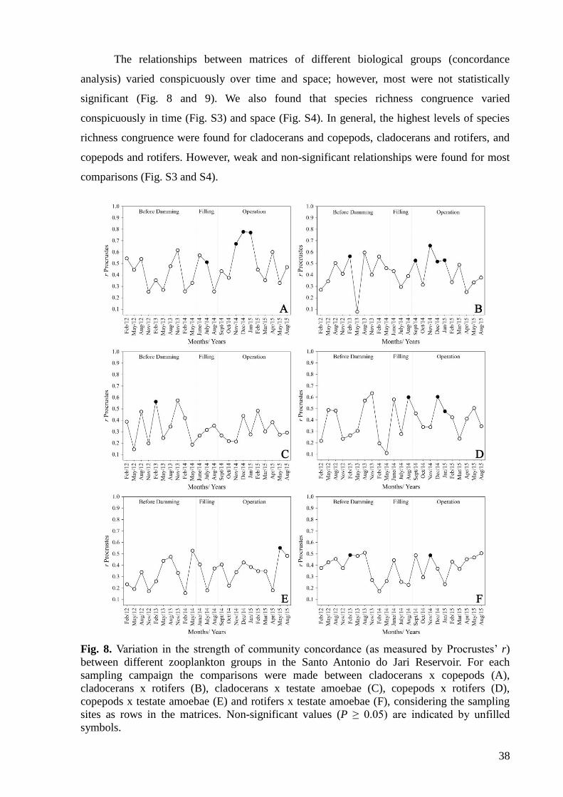
38
The relationships between matrices of different biological groups (concordance
analysis) varied conspicuously over time and space; however, most were not statistically
significant (Fig. 8 and 9). We also found that species richness congruence varied
conspicuously in time (Fig. S3) and space (Fig. S4). In general, the highest levels of species
richness congruence were found for cladocerans and copepods, cladocerans and rotifers, and
copepods and rotifers. However, weak and non-significant relationships were found for most
comparisons (Fig. S3 and S4).
Fig. 8. Variation in the strength of community concordance (as measured by Procrustes’ r)
between different zooplankton groups in the Santo Antonio do Jari Reservoir. For each
sampling campaign the comparisons were made between cladocerans x copepods (A),
cladocerans x rotifers (B), cladocerans x testate amoebae (C), copepods x rotifers (D),
copepods x testate amoebae (E) and rotifers x testate amoebae (F), considering the sampling
sites as rows in the matrices. Non-significant values (P ≥ 0.05) are indicated by unfilled
symbols.
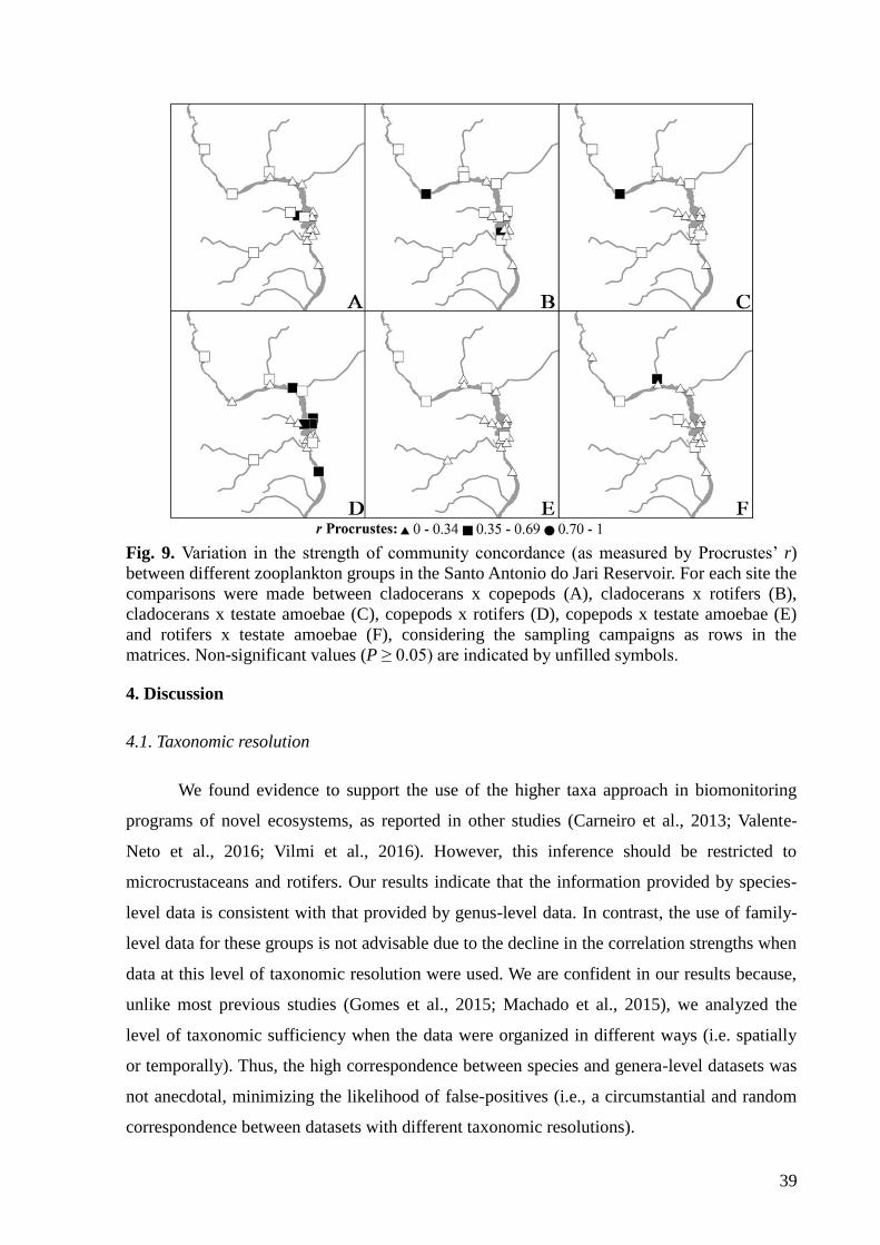
39
Fig. 9. Variation in the strength of community concordance (as measured by Procrustes’ r)
between different zooplankton groups in the Santo Antonio do Jari Reservoir. For each site the
comparisons were made between cladocerans x copepods (A), cladocerans x rotifers (B),
cladocerans x testate amoebae (C), copepods x rotifers (D), copepods x testate amoebae (E)
and rotifers x testate amoebae (F), considering the sampling campaigns as rows in the
matrices. Non-significant values (P ≥ 0.05) are indicated by unfilled symbols.
4. Discussion
4.1. Taxonomic resolution
We found evidence to support the use of the higher taxa approach in biomonitoring
programs of novel ecosystems, as reported in other studies (Carneiro et al., 2013; Valente-
Neto et al., 2016; Vilmi et al., 2016). However, this inference should be restricted to
microcrustaceans and rotifers. Our results indicate that the information provided by species-
level data is consistent with that provided by genus-level data. In contrast, the use of family-
level data for these groups is not advisable due to the decline in the correlation strengths when
data at this level of taxonomic resolution were used. We are confident in our results because,
unlike most previous studies (Gomes et al., 2015; Machado et al., 2015), we analyzed the
level of taxonomic sufficiency when the data were organized in different ways (i.e. spatially
or temporally). Thus, the high correspondence between species and genera-level datasets was
not anecdotal, minimizing the likelihood of false-positives (i.e., a circumstantial and random
correspondence between datasets with different taxonomic resolutions).

40
High correlations for copepods (close to or equal to 1.0) were found in some analyses
due to the similar number of species (10) and genera (8) identified, and the inclusion of larval
forms (nauplii) and juveniles (copepodites) in the analyses (see Rosser, 2017 for a discussion
on the effect of species to higher taxa ratio on taxonomic sufficiency analysis). In practice,
these immature forms are always counted, even when the interest is at the species, genus or
family level. An important reason to consider them is their numerical importance to the
zooplankton community, as these immature forms are often the most abundant among
copepods (Lansac-Tôha et al., 2009). For example, in the present study we recorded 414,905
nauplii and copepodites (85.86%) and only 68,293 adults (14.14%).
The use of a lower taxonomic resolution in biomonitoring programs may be beneficial
in different aspects. First, the sample processing time can be substantially reduced and data
from biological samples can be delivered faster. This is especially valuable in highly dynamic
systems like reservoirs. Second, the resources saved by using a lower taxonomic resolution
can be used instead to expand the biomonitoring program by increasing the number of sites,
the sampling frequency and the number of taxonomic groups monitored. Third, the use of a
lower taxonomic resolution tends to be more robust to variations in the level of expertise of
the personnel involved in a biomonitoring program. For example, in a long-term
biomonitoring program the personnel in charge of the taxonomic determinations will likely
change over time (e.g., due to retirements and job change). Thus, despite standardization
efforts with the new personnel, the differences in taxonomic expertise may be substantial
enough to compromise the comparability of the time series. In this situation, a strong
“change” in community structure over time may simply reflect the change in personnel.
Skepticism regarding the use of a low taxonomic resolution is, however, well-founded
(Maurer, 2000; Verdonschot, 2006; Rosser, 2017). We agree that for basic research (e.g.,
studies on beta diversity), the use of the highest possible level of taxonomic resolution is
needed (Li et al., 2006). Additionally, the effects of subtle environmental impacts may pass
unnoticed with the use of low taxonomic resolution data. However, stronger environmental
changes that are characteristic of reservoirs (e.g., water level variation) are likely to be
detected with low taxonomic resolution data (Bowman and Bailey, 1997; Ferraro and Cole,
1990; Mendes et al., 2007; Wright and Ryan, 2016).
4.2. Numerical resolution
Our results agree with previous studies regarding the negligible information loss
caused by the use of species presence/absence data instead of abundance data, both across

41
temporal and spatial scales. For example, similar results were obtained for phytoplankton
(Carneiro et al., 2010), plants (Landeiro et al., 2012), zooplankton (Gomes et al., 2015) and
macroinvertebrates (Rosa et al., 2014). Similar to the discussion on taxonomic resolution, the
use of a low numerical resolution reduces the sample processing time. We believe that the use
of presence/absence data or partial-abundance data (e.g., Blanchet et al., 2016) can be cost-
effective for monitoring biological communities in reservoirs. However, for specific
applications (e.g., monitoring of harmful algae), abundance data are indispensable.
4.3. Surrogates
Our third prediction was also supported, as we did not find strong and consistent
relationships between the biological matrices of the different zooplankton groups: in general,
the ordination patterns generated for a biological group were unrelated to those generated by a
second group. The results based on congruence in species richness pointed in the same
direction (see also Westgate et al., 2014). Even the relationships between cladocerans and
copepods that are more phylogenetically related to one another than to the other analyzed
groups (see, for example, results from Bini et al., 2008), were often not significant (mean
Procrustes’ r = 0.46; s.d. = 0.15). We agree with Heino (2010) that a much stronger
relationship (> 0.7) would be required to justify the use of a surrogate group as an indicator of
overall biodiversity patterns. In general, our results caution that assessments of the reliability
of surrogate groups based on snapshot surveys may be misleading. For instance, during
December 2014 and January 2015 (operation phase) we found a strong and highly significant
relationship between cladocerans and copepods (r = 0.78 and 0.77, respectively). However,
this result was clearly circumstantial as the strength of the relationships during other sampling
months were low and non-significant. If the evaluation of the reliability of surrogate groups
had been based on this single campaign, the conclusion would have been wrong (see also
Padial et al., 2012). The unreliability of the surrogacy approach is gaining strong support. For
instance, using a meta-analysis that included 15 studies, Westgate et al. (2014) found a very
low average correlation (r = 0.27; s.d. = 0.26). Despite studies indicating the reliability of
surrogate groups (Su et al., 2004), our results suggest, in accordance with a growing body of
evidence (Carneiro et al., 2010; Gioria et al., 2010; Paavola et al., 2003; Ruhí and Batzer,
2014; Vilmi et al., 2016), that this approach should be avoided.
42
5. Conclusion
Reservoirs are novel ecosystems (Turgeon et al., 2016) as complex as natural systems.
Thus, biomonitoring programs for these systems should be designed cautiously. Our results
suggest that the biomonitoring program of the zooplankton community in the SAJHPP based
on genera and presence/absence data is defensible. We speculate that this recommendation
can be extrapolated to other reservoirs in the Amazon region. However, we also recommend
that this strategy be tested first using pilot surveys before it is adopted elsewhere. Once
evidence has been produced to support this recommendation (i.e., the use of zooplankton
genera and presence/absence data), a biomonitoring program, within the context of adaptive
monitoring (Lindenmayer and Likens, 2009), could be reframed to, for instance, increase
sampling frequency and spatial coverage. These are important issues given the high temporal
dynamics and spatial complexity of reservoirs (Kimmel et al., 1990). Finally, our results
suggest that the use of a particular zooplankton group to predict others is unreliable. The
resources saved with the use of cost-effective strategies could then be directed to support the
monitoring of a range of biological groups.
Acknowledgements
We thank Coordenação de Aperfeiçoamento de Pessoal de Nível Superior (CAPES)
and Conselho Nacional de Desenvolvimento Científico e Tecnológico (CNPq) for providing
the master scholarship to MCV, PHD scholarship to LFG and productivity grants to LMB,
LFVM and JCN. CNPq and CAPES have continuously supported our research group in
aquatic ecology. Work by LMB, LCGV and JCN on aquatic ecology have been developed in
the context of National Institutes for Science and Technology (INCT) in Ecology, Evolution
and Biodiversity Conservation, supported by MCTIC/CNpq (proc. 465610/2014-5) and
FAPEG.
REFERENCES
Agostinho, A., Pelicice, F., Gomes, L., 2008. Dams and the fish fauna of the Neotropical
region: impacts and management related to diversity and fisheries. Brazilian J. Biol. 68,
1119–1132. doi:10.1590/S1519-69842008000500019
Backus-Freer, J., Pyron, M., 2015. Concordance among fish and macroinvertebrate
assemblages in streams of Indiana, USA. Hydrobiologia 758, 141–150.
doi:10.1007/s10750-015-2281-6

43
Bae, M.-J., Li, F., Kwon, Y.-S., Chung, N., Choi, H., Hwang, S.-J., Park, Y.-S., 2014.
Concordance of diatom, macroinvertebrate and fish assemblages in streams at nested
spatial scales: Implications for ecological integrity. Ecol. Indic. 47, 89–101.
doi:10.1016/j.ecolind.2014.07.030
Bennett, J.R., Sisson, D.R., Smol, J.P., Cumming, B.F., Possingham, H.P., Buckley, Y.M.,
2014. Optimizing taxonomic resolution and sampling effort to design cost-effective
ecological models for environmental assessment. J. Appl. Ecol. 51, 1722–1732.
doi:10.1111/1365-2664.12312
Bini, L.M., da Silva, L.C.F., Velho, L.F.M., Bonecker, C.C., Lansac-Tôha, F.A., 2008.
Zooplankton assemblage concordance patterns in Brazilian reservoirs. Hydrobiologia
598, 247–255. doi:10.1007/s10750-007-9157-3
Bottrell, H.H., Duncan, A., Gliwicz, Z.M., Grygierek, E., Herzig, A., Hillbrichtilkowska, A.,
Kurasawa, H., Larsson, P., Weglenska, T., 1976. Review of some problems in
zooplankton production studies. Nor. J. Zool. 24, 419–456.
Bowman, M.F., Bailey, R.C., 1997. Does taxonomic resolution affect the multivariate
description of the structure of freshwater benthic macroinvertebrate communities? Can.
J. Fish. Aquat. Sci. 54, 1802–1807. doi:10.1139/f97-085
Bowman, M.F., Ingram, R., Reid, R.A., Somers, K.M., Yan, N.D., Paterson, A.M., Morgan,
G.E., Gunn, J.M., 2008. Temporal and spatial concordance in community composition of
phytoplankton, zooplankton, macroinvertebrate, crayfish, and fish on the Precambrian
Shield. Can. J. Fish. Aquat. Sci. 65, 919–932. doi:10.1139/f08-034
Carneiro, F.M., Bini, L.M., Rodrigues, L.C., 2010. Influence of taxonomic and numerical
resolution on the analysis of temporal changes in phytoplankton communities. Ecol.
Indic. 10, 249–255. doi:10.1016/j.ecolind.2009.05.004
Carneiro, F.M., Nabout, J.C., Vieira, L.C.G., Lodi, S., Bini, L.M., 2013. Higher Taxa Predict
Plankton Beta-diversity Patterns Across an Eutrophication Gradient. Nat. Conserv. 11,
43–47. doi:10.4322/natcon.2013.006
Corte, G.N., Checon, H.H., Fonseca, G., Vieira, D.C., Gallucci, F., Di Domenico,
M. and Amaral, A.C.Z., 2017. Cross-
taxon congruence in benthiccommunities: Searching for surrogates in
44
marine sediments. Ecol. Indic., 78, 173-182.
Dudgeon, D., Arthington, A.H., Gessner, M.O., Kawabata, Z.-I., Knowler, D.J., Lévêque, C.,
Naiman, R.J., Prieur-Richard, A.-H., Soto, D., Stiassny, M.L.J., Sullivan, C.A., 2006.
Freshwater biodiversity: importance, threats, status and conservation challenges. Biol.
Rev. 81, 163. doi:10.1017/S1464793105006950
Ferraro, S., Cole, F., 1990. Taxonomic level and sample size sufficient for assessing pollution
impacts on the Southern California Bight macro-benthos. Mar. Ecol. Prog. Ser. 67, 251–
262. doi:10.3354/meps067251
Gioria, M., Schaffers, A., Bacaro, G., Feehan, J., 2010. The conservation value of farmland
ponds: Predicting water beetle assemblages using vascular plants as a surrogate group.
Biol. Conserv. 143, 1125–1133. doi:10.1016/j.biocon.2010.02.007
Gomes, L.F., Vieira, L.C.G., Bonnet, M.P., 2015. Two practical approaches to monitoring the
zooplanktonic community at Lago Grande do Curuai, Pará, Brazil. Acta Amaz. 45, 293–
298. doi:10.1590/1809-4392201404453
Grenouillet, G., Brosse, S., Tudesque, L., Lek, S., Baraillé, Y., Loot, G., 2008. Concordance
among stream assemblages and spatial autocorrelation along a fragmented gradient.
Divers. Distrib. 14, 592–603. doi:10.1111/j.1472-4642.2007.00443.x
Guareschi, S., Abellán, P., Laini, A., Green, A.J., Sánchez-Zapata, J.A., Velasco, J., Millán, A.,
2015. Cross-taxon congruence in wetlands: Assessing the value of waterbirds as
surrogates of macroinvertebrate biodiversity in Mediterranean Ramsar sites. Ecol. Indic.
49, 204–215. doi:10.1016/j.ecolind.2014.10.012
Blanchet, F.G., Legendre, P., He, F., 2016. A new cost-effective approach to survey ecological
communities. Oikos 125, 975–987. doi:10.1111/oik.02838
Heino, J., 2014. Taxonomic surrogacy, numerical resolution and responses of stream
macroinvertebrate communities to ecological gradients: Are the inferences transferable
among regions? Ecol. Indic. 36, 186–194. doi:10.1016/j.ecolind.2013.07.022
Heino, J., 2010. Are indicator groups and cross-taxon congruence useful for predicting
biodiversity in aquatic ecosystems? Ecol. Indic. 10, 112–117.
doi:10.1016/j.ecolind.2009.04.013
45
Hobbs, R.J., Arico, S., Aronson, J., Baron, J.S., Bridgewater, P., Cramer, V.A., Epstein, P.R.,
Ewel, J.J., Klink, C.A., Lugo, A.E., Norton, D., Ojima, D., Richardson, D.M., Sanderson,
E.W., Valladares, F., Vila, M., Zamora, R., Zobel, M., 2006. Novel ecosystems:
theoretical and management aspects of the new ecological world order. Glob. Ecol.
Biogeogr. 15, 1–7. doi:10.1111/j.1466-822X.2006.00212.x
Hobbs, R.J., Higgs, E., Harris, J.A., 2009. Novel ecosystems: implications for conservation
and restoration. Trends Ecol. Evol. 24, 599–605. doi:10.1016/j.tree.2009.05.012
Jiang, Y., Liu, Q., Yang, E.J., Wang, M., Lee, Y., Lee, S., 2016. An approach to bioassess
pelagic ciliate biodiversity at different taxonomic resolutions in response to various
habitats in the Amundsen Sea (Antarctica). Polar Biol. 39, 485–495.
doi:10.1007/s00300-015-1801-1
Joseph, L.N., Field, S.A., Wilcox, C., Possingham, H.P., 2006. Presence-Absence versus
Abundance Data for Monitoring Threatened Species. Conserv. Biol. 20, 1679–1687.
doi:10.1111/j.1523-1739.2006.00529.x
Kallimanis, A.S., Mazaris, A.D., Tsakanikas, D., Dimopoulos, P., Pantis, J.D., Sgardelis, S.P.,
2012. Efficient biodiversity monitoring: Which taxonomic level to study? Ecol. Indic.
15, 100–104. doi:10.1016/j.ecolind.2011.09.024
Kilgour, B.W., Barton, D.R., 1999. Associations between stream fish and benthos across
environmental gradients in southern Ontario, Canada. Freshw. Biol. 41, 553–566.
doi:10.1046/j.1365-2427.1999.00402.x
Kimmel, B.L., Lind, O.T., Paulson, L.J., 1990. Reservoir primary production, in: Thornton,
K.W., Kimmel, B.L., Payne, F.E. (Eds.), Reservoir Limnology: Ecological Perspectives.
Wiley, pp. 133–194.
Kimmel, W.G., Argent, D., 2016. Community concordance between fishes and benthic
macroinvertebrates among adventitious and ordinate tributaries of a major river system.
Ecol. Indic. 70, 15–22. doi:10.1016/j.ecolind.2016.05.037
Lansac-Tôha, F. A., Bonecker, C. C., Velho, L. F. M., Simões, N. R., Dias, J. D., Alves, G. M.,
Takahashi, E. M., 2009. Biodiversity of zooplankton communities in the Upper Paraná
River floodplain: interannual variation from long-term studies. Braz. J. Biol. 69, 539-
549. dx.doi.org/10.1590/S1519-69842009000300009
46
Landeiro, V.L., Bini, L.M., Costa, F.R.C., Franklin, E., Nogueira, A., de Souza, J.L.P.,
Moraes, J., Magnusson, W.E., 2012. How far can we go in simplifying biomonitoring
assessments? An integrated analysis of taxonomic surrogacy, taxonomic sufficiency and
numerical resolution in a megadiverse region. Ecol. Indic. 23, 366–373.
doi:10.1016/j.ecolind.2012.04.023
Legendre, P., Gallagher, E., 2001. Ecologically meaningful transformations for ordination of
species data. Oecologia 129, 271–280. doi:10.1007/s004420100716
Legendre, P., Legendre, L., 2012. Numerical ecology, Third edit. ed. Elsevier.
Li, Z., Yu, D., Xiong, W., Wang, Q., Tu, M., 2006. Testing the higher-taxon approach: a case
study of aquatic marcophytes in China’s northwest arid zone and its implications for
conservation. Biodivers. Conserv. 15, 3401–3416. doi:10.1007/s10531-004-8228-2
Lindenmayer, D.B., Likens, G.E., 2009. Adaptive monitoring: a new paradigm for long-term
research and monitoring. Trends Ecol. Evol. 24, 482–486. doi:10.1016/j.tree.2009.03.005
Lodi, S., Velho, L.F.M., Carvalho, P., Bini, L.M., 2014. Patterns of zooplankton population
synchrony in a tropical reservoir. J. Plankton Res. 36, 966–977.
doi:10.1093/plankt/fbu028
Lovell, S., Hamer, M., Slotow, R., Herbert, D., 2007. Assessment of congruency across
invertebrate taxa and taxonomic levels to identify potential surrogates. Biol. Conserv.
139, 113–125. doi:10.1016/j.biocon.2007.06.008
Machado, K.B., Borges, P.P., Carneiro, F.M., de Santana, J.F., Vieira, L.C.G., de Moraes
Huszar, V.L., Nabout, J.C., 2015. Using lower taxonomic resolution and ecological
approaches as a surrogate for plankton species. Hydrobiologia 743, 255–267.
doi:10.1007/s10750-014-2042-y
Marshall, J.C., Steward, A.L., Harch, B.D., 2006. Taxonomic Resolution and Quantification
of Freshwater Macroinvertebrate Samples from an Australian Dryland River: The
Benefits and Costs of Using Species Abundance Data. Hydrobiologia 572, 171–194.
doi:10.1007/s10750-005-9007-0
Maurer, D., 2000. The Dark Side of Taxonomic Sufficiency (TS). Mar. Pollut. Bull. 40, 98–
101. doi:10.1016/S0025-326X(99)00235-0

47
Mazón, M., 2016. Taking shortcuts to measure species diversity: parasitoid Hymenoptera
subfamilies as surrogates of species richness. Biodivers. Conserv. 25, 67–76.
doi:10.1007/s10531-015-1029-y
Melo, A.S., 2005. Effects of taxonomic and numeric resolution on the ability to detect
ecological patterns at a local scale using stream macroinvertebrates. Arch. für Hydrobiol.
164, 309–323. doi:10.1127/0003-9136/2005/0164-0309
Mendes, C.L.T., Tavares, M., Soares-Gomes, A., 2007. Taxonomic sufficiency for soft-bottom
sublittoral mollusks assemblages in a tropical estuary, Guanabara Bay, Southeast Brazil.
Mar. Pollut. Bull. 54, 377–384. doi:10.1016/j.marpolbul.2006.08.026
Oksanen, J., Blanchet, F.G., Friendly, M., Kindt, R., Legendre, P., Mcglinn, D., Minchin, P.R.,
O ’hara, R.B., Simpson, G.L., Solymos, P., Stevens, H., Szoecs, E., Wagner, H., 2016.
Vegan: Community Ecology Package. R Packag. version 2.4-0.
Paavola, R., Muotka, T., Virtanen, R., Heino, J., Jackson, D., Mäki-Petäys, A., 2006. Spatial
Scale Affects Community Concordance Among Fishes, Benthic Macroinvertebrates, And
Bryophytes In Streams. Ecol. Appl. 16, 368–379. doi:10.1890/03-5410
Paavola, R., Muotka, T., Virtanen, R., Heino, J., Kreivi, P., 2003. Are biological classifications
of headwater streams concordant across multiple taxonomic groups? Freshw. Biol. 48,
1912–1923. doi:10.1046/j.1365-2427.2003.01131.x
Padial, A. a., Declerck, S.A.J., De Meester, L., Bonecker, C.C., Lansac-Tôha, F. a., Rodrigues,
L.C., Takeda, A., Train, S., Velho, L.F.M., Bini, L.M., 2012. Evidence against the use of
surrogates for biomonitoring of Neotropical floodplains. Freshw. Biol. 57, 2411–2423.
doi:10.1111/fwb.12008
R Core Team, 2017. R: A Language and Environment for Statistical Computing.
Rosa, B.J.F.V., Rodrigues, L.F.T., de Oliveira, G.S., da Gama Alves, R., 2014. Chironomidae
and Oligochaeta for water quality evaluation in an urban river in southeastern Brazil.
Environ. Monit. Assess. 186, 7771–7779. doi:10.1007/s10661-014-3965-5
Rosser, N., 2017. Shortcuts in biodiversity research: What determines the performance of
higher taxa as surrogates for species? Ecol. Evol. 7, 2595-2603. doi:10.1002/ece3.2736
Ruhí, A., Batzer, D.P., 2014. Assessing Congruence and Surrogacy Among Wetland
48
Macroinvertebrate Taxa Towards Efficiently Measuring Biodiversity. Wetlands 34,
1061–1071. doi:10.1007/s13157-014-0566-6
Sánchez-Moyano, J.E., Fa, D.A., Estacio, F.J., García-Gómez, J.C., 2006. Monitoring of
marine benthic communities and taxonomic resolution: an approach through diverse
habitats and substrates along the Southern Iberian coastline. Helgol. Mar. Res. 60, 243–
255. doi:10.1007/s10152-006-0039-2
Seastedt, T.R., Hobbs, R.J., Suding, K.N., 2008. Management of novel ecosystems: are novel
approaches required? Front. Ecol. Environ. 6, 547–553. doi:10.1890/070046
Silva, L.H.S., Huszar, V.L.M., Marinho, M.M., Rangel, L.M., Brasil, J., Domingues, C.D.,
Branco, C.C., Roland, F., 2014. Drivers of phytoplankton, bacterioplankton, and
zooplankton carbon biomass in tropical hydroelectric reservoirs. Limnol. - Ecol. Manag.
Inl. Waters 48, 1–10. doi:10.1016/j.limno.2014.04.004
Simões, N.R., Nunes, A.H., Dias, J.D., Lansac-Tôha, F.A., Velho, L.F.M., Bonecker, C.C.,
2015. Impact of reservoirs on zooplankton diversity and implications for the
conservation of natural aquatic environments. Hydrobiologia 758, 3–17.
doi:10.1007/s10750-015-2260-y
Su, J.C., Debinsky, D.M., Jakubauskas, M.E., Kindscher, K., 2004. Beyond Species Richness:
Community Similarity as a Measure of Cross-Taxon Congruence for Coarse-Filter
Conservation. Conserv. Biol. 18, 167–173. doi:10.1111/j.1523-1739.2004.00337.x
Turgeon, K., Solomon, C.T., Nozais, C., Gregory-Eaves, I., 2016. Do novel ecosystems
follow predictable trajectories? Testing the trophic surge hypothesis in reservoirs using
fish. Ecosphere 7, e01617. doi:10.1002/ecs2.1617
Valente-Neto, F., De Oliveira Roque, F., Rodrigues, M.E., Juen, L., Swan, C.M., 2016.
Toward a practical use of Neotropical odonates as bioindicators: Testing congruence
across taxonomic resolution and life stages. Ecol. Indic. 61, 952–959.
doi:10.1016/j.ecolind.2015.10.052
Verdonschot, P.F.M., 2006. Data composition and taxonomic resolution in macroinvertebrate
stream typology. Hydrobiologia 566, 59–74. doi:10.1007/s10750-006-0070-y
Vilmi, A., Karjalainen, S.M., Nokela, T., Tolonen, K., Heino, J., 2016. Unravelling the drivers
of aquatic communities using disparate organismal groups and different taxonomic
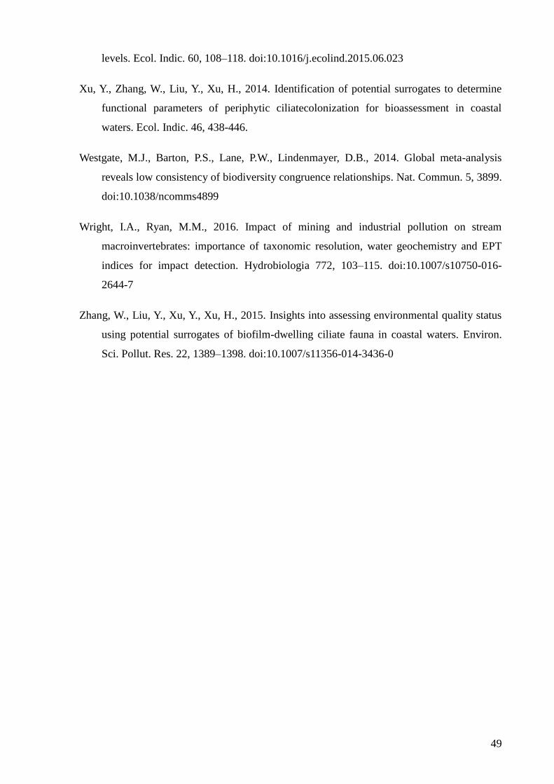
49
levels. Ecol. Indic. 60, 108–118. doi:10.1016/j.ecolind.2015.06.023
Xu, Y., Zhang, W., Liu, Y., Xu, H., 2014. Identification of potential surrogates to determine
functional parameters of periphytic ciliatecolonization for bioassessment in coastal
waters. Ecol. Indic. 46, 438-446.
Westgate, M.J., Barton, P.S., Lane, P.W., Lindenmayer, D.B., 2014. Global meta-analysis
reveals low consistency of biodiversity congruence relationships. Nat. Commun. 5, 3899.
doi:10.1038/ncomms4899
Wright, I.A., Ryan, M.M., 2016. Impact of mining and industrial pollution on stream
macroinvertebrates: importance of taxonomic resolution, water geochemistry and EPT
indices for impact detection. Hydrobiologia 772, 103–115. doi:10.1007/s10750-016-
2644-7
Zhang, W., Liu, Y., Xu, Y., Xu, H., 2015. Insights into assessing environmental quality status
using potential surrogates of biofilm-dwelling ciliate fauna in coastal waters. Environ.
Sci. Pollut. Res. 22, 1389–1398. doi:10.1007/s11356-014-3436-0
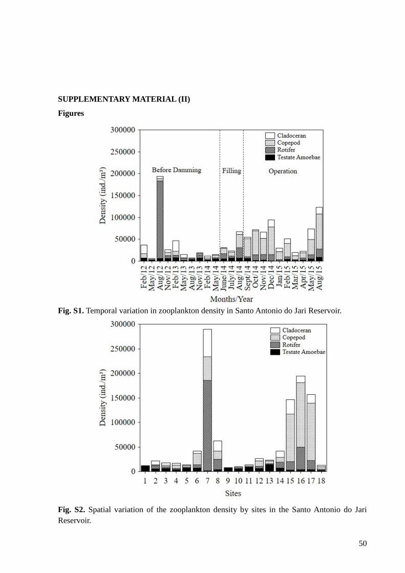
50
SUPPLEMENTARY MATERIAL (II)
Figures
Fig. S1. Temporal variation in zooplankton density in Santo Antonio do Jari Reservoir.
Fig. S2. Spatial variation of the zooplankton density by sites in the Santo Antonio do Jari
Reservoir.

51
Fig. S3. Variation in the strength of the cross-taxon correlation in species richness (as
measured by Spearman's ρ) between different zooplankton groups in Santo Antonio do Jari
Reservoir. For each sampling campaign the comparisons were made between cladocerans x
copepods (A), cladocerans x rotifers (B), cladocerans x testate amoebae (C), copepods x
rotifers (D), copepods x testate amoebae (E) and rotifers x testate amoebae (F), considering
the sampling sites as rows in the matrices. Non-significant values (P ≥ 0.05) are indicated by
unfilled symbols.
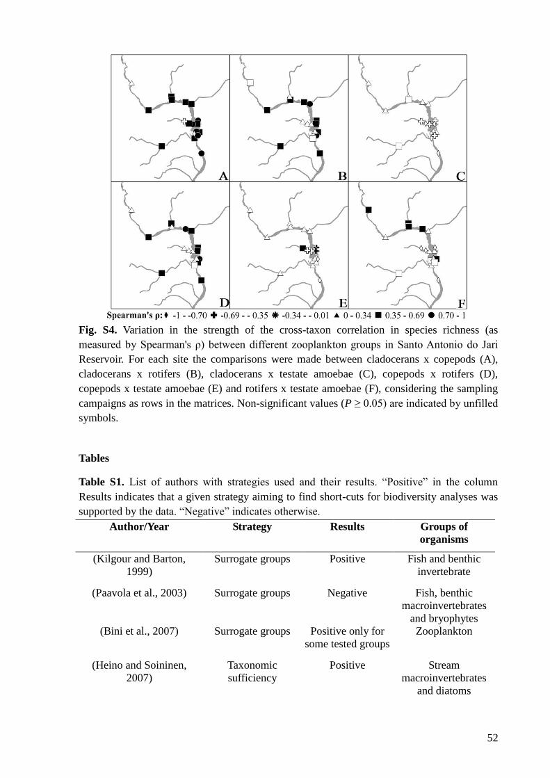
52
Fig. S4. Variation in the strength of the cross-taxon correlation in species richness (as
measured by Spearman's ρ) between different zooplankton groups in Santo Antonio do Jari
Reservoir. For each site the comparisons were made between cladocerans x copepods (A),
cladocerans x rotifers (B), cladocerans x testate amoebae (C), copepods x rotifers (D),
copepods x testate amoebae (E) and rotifers x testate amoebae (F), considering the sampling
campaigns as rows in the matrices. Non-significant values (P ≥ 0.05) are indicated by unfilled
symbols.
Tables
Table S1. List of authors with strategies used and their results. “Positive” in the column
Results indicates that a given strategy aiming to find short-cuts for biodiversity analyses was
supported by the data. “Negative” indicates otherwise.
Author/Year Strategy Results Groups of
organisms
(Kilgour and Barton,
1999)
Surrogate groups Positive Fish and benthic
invertebrate
(Paavola et al., 2003) Surrogate groups Negative Fish, benthic
macroinvertebrates
and bryophytes
(Bini et al., 2007) Surrogate groups Positive only for
some tested groups
Zooplankton
(Heino and Soininen,
2007)
Taxonomic
sufficiency
Positive Stream
macroinvertebrates
and diatoms
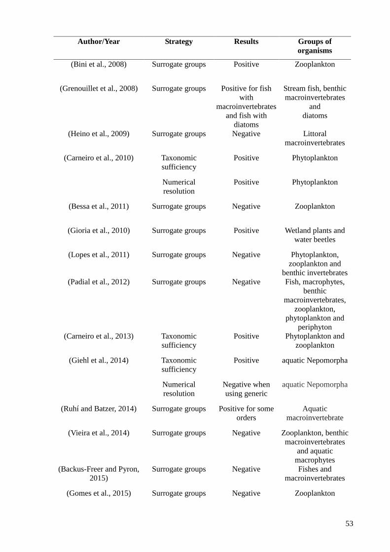
53
Author/Year Strategy Results Groups of
organisms
(Bini et al., 2008) Surrogate groups Positive Zooplankton
(Grenouillet et al., 2008) Surrogate groups Positive for fish
with
macroinvertebrates
and fish with
diatoms
Stream fish, benthic
macroinvertebrates
and
diatoms
(Heino et al., 2009) Surrogate groups Negative Littoral
macroinvertebrates
(Carneiro et al., 2010) Taxonomic
sufficiency
Positive Phytoplankton
Numerical
resolution
Positive Phytoplankton
(Bessa et al., 2011) Surrogate groups Negative Zooplankton
(Gioria et al., 2010) Surrogate groups Positive Wetland plants and
water beetles
(Lopes et al., 2011) Surrogate groups Negative Phytoplankton,
zooplankton and
benthic invertebrates
(Padial et al., 2012) Surrogate groups Negative Fish, macrophytes,
benthic
macroinvertebrates,
zooplankton,
phytoplankton and
periphyton
(Carneiro et al., 2013) Taxonomic
sufficiency
Positive Phytoplankton and
zooplankton
(Giehl et al., 2014) Taxonomic
sufficiency
Positive aquatic Nepomorpha
Numerical
resolution
Negative when
using generic
aquatic Nepomorpha
(Ruhí and Batzer, 2014) Surrogate groups Positive for some
orders
Aquatic
macroinvertebrate
(Vieira et al., 2014) Surrogate groups Negative Zooplankton, benthic
macroinvertebrates
and aquatic
macrophytes
(Backus-Freer and Pyron,
2015)
Surrogate groups Negative Fishes and
macroinvertebrates
(Gomes et al., 2015) Surrogate groups Negative Zooplankton
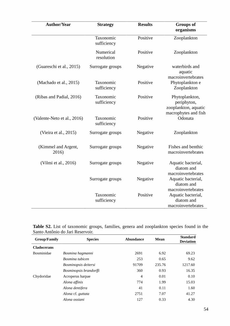
54
Author/Year Strategy Results Groups of
organisms
Taxonomic
sufficiency
Positive Zooplankton
Numerical
resolution
Positive Zooplankton
(Guareschi et al., 2015) Surrogate groups Negative waterbirds and
aquatic
macroinvertebrates
(Machado et al., 2015) Taxonomic
sufficiency
Positive Phytoplankton e
Zooplankton
(Ribas and Padial, 2016) Taxonomic
sufficiency
Positive Phytoplankton,
periphyton,
zooplankton, aquatic
macrophytes and fish
(Valente-Neto et al., 2016) Taxonomic
sufficiency
Positive Odonata
(Vieira et al., 2015) Surrogate groups Negative Zooplankton
(Kimmel and Argent,
2016)
Surrogate groups Negative Fishes and benthic
macroinvertebrates
(Vilmi et al., 2016) Surrogate groups Negative Aquatic bacterial,
diatom and
macroinvertebrates
Surrogate groups Negative Aquatic bacterial,
diatom and
macroinvertebrates
Taxonomic
sufficiency
Positive Aquatic bacterial,
diatom and
macroinvertebrates
Table S2. List of taxonomic groups, families, genera and zooplankton species found in the
Santo Antônio do Jari Reservoir.
Group/Family Species Abundance Mean Standard
Deviation
Cladocerans
Bosminidae Bosmina hagmanni 2691 6.92 69.23
Bosmina tubicen 253 0.65 9.62
Bosminopsis deitersi 91709 235.76 1217.60
Bosminopsis brandorffi 360 0.93 16.35
Chydoridae Acroperus harpae 4 0.01 0.10
Alona affinis 774 1.99 15.03
Alona dentifera 41 0.11 1.60
Alona cf. guttata 2751 7.07 41.27
Alona ossiani 127 0.33 4.30
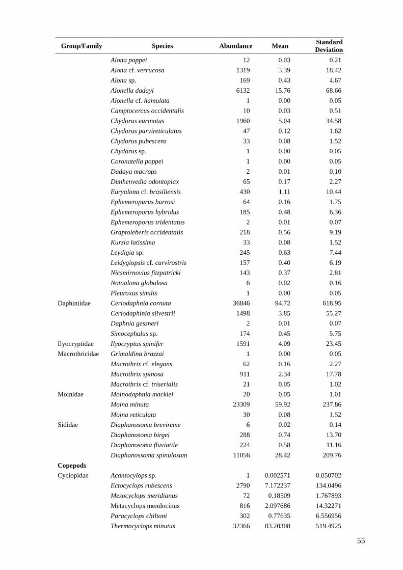
55
Group/Family Species Abundance Mean Standard
Deviation
Alona poppei 12 0.03 0.21
Alona cf. verrucosa 1319 3.39 18.42
Alona sp. 169 0.43 4.67
Alonella dadayi 6132 15.76 68.66
Alonella cf. hamulata 1 0.00 0.05
Camptocercus occidentalis 10 0.03 0.51
Chydorus eurinotus 1960 5.04 34.58
Chydorus parvireticulatus 47 0.12 1.62
Chydorus pubescens 33 0.08 1.52
Chydorus sp. 1 0.00 0.05
Coronatella poppei 1 0.00 0.05
Dadaya macrops 2 0.01 0.10
Dunhenvedia odontoplax 65 0.17 2.27
Euryalona cf. brasiliensis 430 1.11 10.44
Ephemeropurus barrosi 64 0.16 1.75
Ephemeroporus hybridus 185 0.48 6.36
Ephemeroporus tridentatus 2 0.01 0.07
Graptoleberis occidentalis 218 0.56 9.19
Kurzia latissima 33 0.08 1.52
Leydigia sp. 245 0.63 7.44
Leidygiopsis cf. curvirostris 157 0.40 6.19
Nicsmirnovius fitzpatricki 143 0.37 2.81
Notoalona globulosa 6 0.02 0.16
Pleuroxus similis 1 0.00 0.05
Daphiniidae Ceriodaphnia cornuta 36846 94.72 618.95
Ceriodaphinia silvestrii 1498 3.85 55.27
Daphnia gessneri 2 0.01 0.07
Simocephalus sp. 174 0.45 5.75
Ilyocryptidae Ilyocryptus spinifer 1591 4.09 23.45
Macrothricidae Grimaldina brazzai 1 0.00 0.05
Macrothrix cf. elegans 62 0.16 2.27
Macrothrix spinosa 911 2.34 17.78
Macrothrix cf. triserialis 21 0.05 1.02
Moinidae Moinodaphnia macklei 20 0.05 1.01
Moina minuta 23309 59.92 237.86
Moina reticulata 30 0.08 1.52
Sididae Diaphanosoma brevireme 6 0.02 0.14
Diaphanosoma birgei 288 0.74 13.70
Diaphanosoma fluviatile 224 0.58 11.16
Diaphanossoma spinulosum 11056 28.42 209.76
Copepods
Cyclopidae Acantocylops sp. 1 0.002571 0.050702
Ectocyclops rubescens 2790 7.172237 134.0496
Mesocyclops meridianus 72 0.18509 1.767893
Metacyclops mendocinus 816 2.097686 14.32271
Paracyclops chiltoni 302 0.77635 6.556956
Thermocyclops minutus 32366 83.20308 519.4925
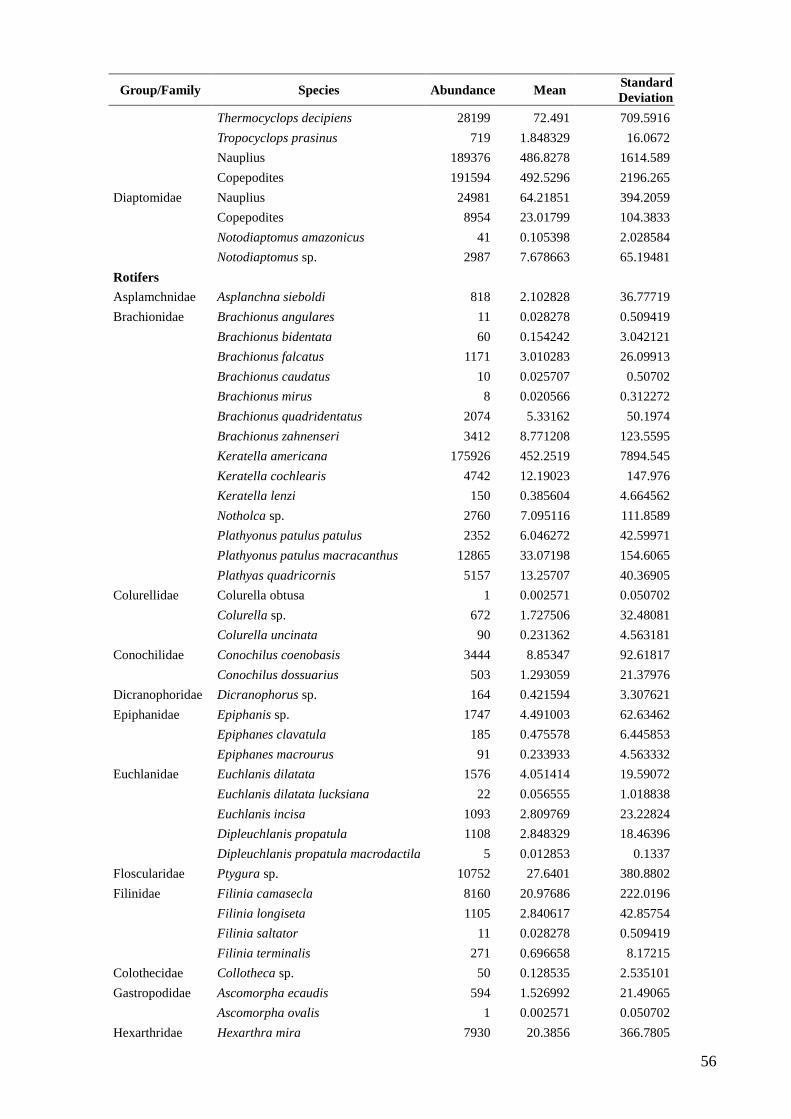
56
Group/Family Species Abundance Mean Standard
Deviation
Thermocyclops decipiens 28199 72.491 709.5916
Tropocyclops prasinus 719 1.848329 16.0672
Nauplius 189376 486.8278 1614.589
Copepodites 191594 492.5296 2196.265
Diaptomidae Nauplius 24981 64.21851 394.2059
Copepodites 8954 23.01799 104.3833
Notodiaptomus amazonicus 41 0.105398 2.028584
Notodiaptomus sp. 2987 7.678663 65.19481
Rotifers
Asplamchnidae Asplanchna sieboldi 818 2.102828 36.77719
Brachionidae Brachionus angulares 11 0.028278 0.509419
Brachionus bidentata 60 0.154242 3.042121
Brachionus falcatus 1171 3.010283 26.09913
Brachionus caudatus 10 0.025707 0.50702
Brachionus mirus 8 0.020566 0.312272
Brachionus quadridentatus 2074 5.33162 50.1974
Brachionus zahnenseri 3412 8.771208 123.5595
Keratella americana 175926 452.2519 7894.545
Keratella cochlearis 4742 12.19023 147.976
Keratella lenzi 150 0.385604 4.664562
Notholca sp. 2760 7.095116 111.8589
Plathyonus patulus patulus 2352 6.046272 42.59971
Plathyonus patulus macracanthus 12865 33.07198 154.6065
Plathyas quadricornis 5157 13.25707 40.36905
Colurellidae Colurella obtusa 1 0.002571 0.050702
Colurella sp. 672 1.727506 32.48081
Colurella uncinata 90 0.231362 4.563181
Conochilidae Conochilus coenobasis 3444 8.85347 92.61817
Conochilus dossuarius 503 1.293059 21.37976
Dicranophoridae Dicranophorus sp. 164 0.421594 3.307621
Epiphanidae Epiphanis sp. 1747 4.491003 62.63462
Epiphanes clavatula 185 0.475578 6.445853
Epiphanes macrourus 91 0.233933 4.563332
Euchlanidae Euchlanis dilatata 1576 4.051414 19.59072
Euchlanis dilatata lucksiana 22 0.056555 1.018838
Euchlanis incisa 1093 2.809769 23.22824
Dipleuchlanis propatula 1108 2.848329 18.46396
Dipleuchlanis propatula macrodactila 5 0.012853 0.1337
Floscularidae Ptygura sp. 10752 27.6401 380.8802
Filinidae Filinia camasecla 8160 20.97686 222.0196
Filinia longiseta 1105 2.840617 42.85754
Filinia saltator 11 0.028278 0.509419
Filinia terminalis 271 0.696658 8.17215
Colothecidae Collotheca sp. 50 0.128535 2.535101
Gastropodidae Ascomorpha ecaudis 594 1.526992 21.49065
Ascomorpha ovalis 1 0.002571 0.050702
Hexarthridae Hexarthra mira 7930 20.3856 366.7805

57
Group/Family Species Abundance Mean Standard
Deviation
Hexarthra intermedia 7500 19.28021 380.2651
Hexarthra sp. 32 0.082262 1.522484
Lecanidae Lecane bulla 6524 16.77121 74.36897
Lecane curvicornis 2659 6.835476 30.77343
Lecane closterocerca 84 0.215938 2.479743
Lecane cornuta 1213 3.118252 22.43803
Lecane elsa 2 0.005141 0.101404
Lecane cf. halyclista 30 0.077121 1.52106
Lecane hamata 1 0.002571 0.050702
Lecane hornemanni 30 0.077121 1.52106
Lecane leontina 3991 10.25964 87.76769
Lecane ludwigi 207 0.532134 6.481307
Lecane luna 5578 14.33933 61.114
Lecane lunaris 1336 3.434447 26.91853
Lecane monostyla 6285 16.15681 207.024
Lecane quadridentata 1578 4.056555 26.71763
Lecane papuana 1158 2.976864 26.03026
Lecane proiecta 11 0.028278 0.509419
Lecane signifera 2 0.005141 0.071611
Lecane stenroosi 10 0.025707 0.50702
Lecane sp. 234 0.601542 6.68959
Lepadellidae Lepadella acuminata 1 0.002571 0.050702
Lepadella benjamini 252 0.647815 8.424735
Lepadella cristata 2 0.005141 0.071611
Lepadella ovalis 304 0.781491 4.621339
Lepadella patela 970 2.493573 15.92453
Mytilinidae Mytilina macrocera 395 1.015424 9.102213
Mytilina sp. 62 0.159383 3.042702
Mytillina cf. ventralis 109 0.280206 2.578888
Bdelloidea Bdelloidea 9238 23.74807 84.42021
Proalidae Proales sp. 77 0.197943 2.32299
Notommatidae Notommata copeus 36 0.092545 0.883217
Notommata sp. 77 0.197943 2.32299
Cephalodella mucronata 3 0.007712 0.152106
Cephalodella sp. 111 0.285347 1.886828
Monommata sp. 1 0.002571 0.050702
Synchaetidae Ploesoma truncatum 122 0.313625 6.084402
Polyarthra dolichoptera 7435 19.11311 244.9637
Polyarthra vulgaris 12603 32.39846 332.3855
Synchaeta pectinata 1954 5.023136 44.06792
Testudinellidae Testudinella patina 1741 4.475578 20.75278
Testudinella mucronata 487 1.251928 9.486196
Testudinella tridentata 2 0.005141 0.071611
Trichotridae Macrochaetus collinsi 1 0.002571 0.050702
Macrochaetus sericus 105 0.269923 4.590628
Trichotria tetractis 395 1.015424 9.390979
Trichocercidae Trichocerca bicristata 550 1.413882 14.51966
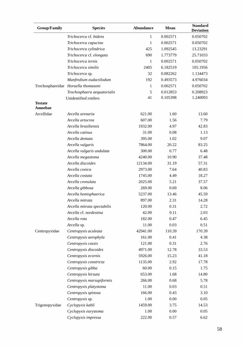
58
Group/Family Species Abundance Mean Standard
Deviation
Trichocerca cf. bidens 1 0.002571 0.050702
Trichocerca capucina 1 0.002571 0.050702
Trichocerca cylindrica 425 1.092545 13.23291
Trichocerca cf. elongata 690 1.773779 25.71033
Trichocerca iernis 1 0.002571 0.050702
Trichocerca similis 2405 6.182519 105.1956
Trichocerca sp. 32 0.082262 1.134473
Manfredium eudactilodum 192 0.493573 4.976034
Trochosphaeridae Horaella thomasoni 1 0.002571 0.050702
Trochosphaera aequatorialis 5 0.012853 0.208923
Unidentified rotifers 41 0.105398 1.240093
Testate
Amoebae
Arcellidae Arcella arenaria 621.00 1.60 13.60
Arcella artocrea 607.00 1.56 7.79
Arcella brasiliensis 1932.00 4.97 42.83
Arcella catinus 31.00 0.08 1.13
Arcella dentata 395.00 1.02 9.07
Arcella vulgaris 7864.00 20.22 83.25
Arcella vulgaris undulata 300.00 0.77 6.48
Arcella megastoma 4240.00 10.90 37.48
Arcella discoides 12134.00 31.19 57.31
Arcella conica 2973.00 7.64 40.83
Arcella costata 1745.00 4.49 18.27
Arcella crenulata 2025.00 5.21 37.57
Arcella gibbosa 269.00 0.69 8.06
Arcella hemisphaerica 5237.00 13.46 45.59
Arcella mitrata 897.00 2.31 14.28
Arcella mitrata spectabilis 120.00 0.31 2.72
Arcella cf. nordestina 42.00 0.11 2.03
Arcella rota 182.00 0.47 6.45
Arcella sp. 11.00 0.03 0.51
Centropyxidae Centropyxis aculeata 42941.00 110.39 170.39
Centropyxis aerophyla 161.00 0.41 4.38
Centropyxis cassis 121.00 0.31 2.76
Centropyxis discoides 4971.00 12.78 33.53
Centropyxis ecornis 5926.00 15.23 41.18
Centropyxis constricta 1135.00 2.92 17.78
Centropyxis gibba 60.00 0.15 1.75
Centropyxis hirsuta 653.00 1.68 14.80
Centropyxis marsupiformis 266.00 0.68 5.78
Centropyxis platystoma 11.00 0.03 0.51
Centropyxis spinosa 166.00 0.43 3.10
Centropyxis sp. 1.00 0.00 0.05
Trigonopyxidae Cyclopyxis kahli 1459.00 3.75 14.53
Cyclopyxis eurystoma 1.00 0.00 0.05
Cyclopyxis impressa 222.00 0.57 6.62
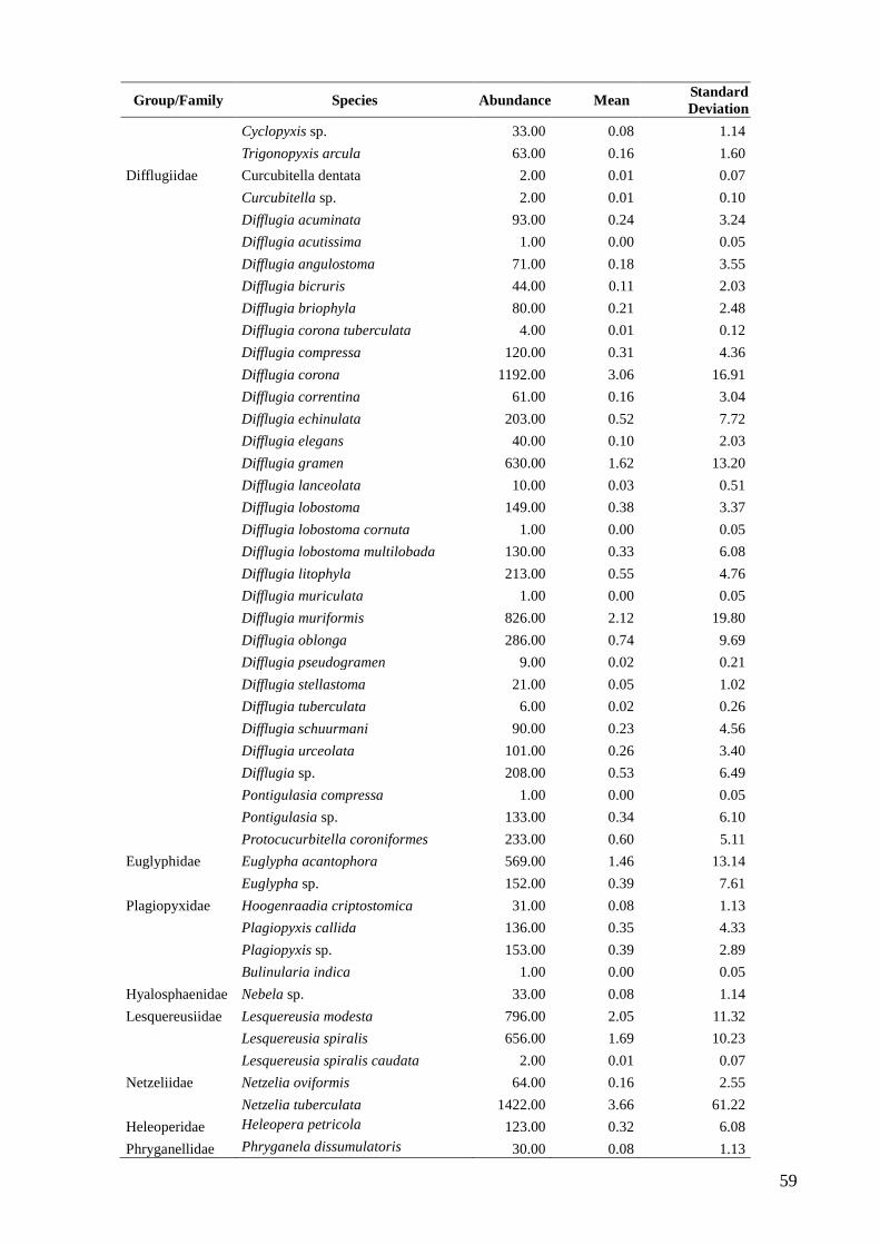
59
Group/Family Species Abundance Mean Standard
Deviation
Cyclopyxis sp. 33.00 0.08 1.14
Trigonopyxis arcula 63.00 0.16 1.60
Difflugiidae Curcubitella dentata 2.00 0.01 0.07
Curcubitella sp. 2.00 0.01 0.10
Difflugia acuminata 93.00 0.24 3.24
Difflugia acutissima 1.00 0.00 0.05
Difflugia angulostoma 71.00 0.18 3.55
Difflugia bicruris 44.00 0.11 2.03
Difflugia briophyla 80.00 0.21 2.48
Difflugia corona tuberculata 4.00 0.01 0.12
Difflugia compressa 120.00 0.31 4.36
Difflugia corona 1192.00 3.06 16.91
Difflugia correntina 61.00 0.16 3.04
Difflugia echinulata 203.00 0.52 7.72
Difflugia elegans 40.00 0.10 2.03
Difflugia gramen 630.00 1.62 13.20
Difflugia lanceolata 10.00 0.03 0.51
Difflugia lobostoma 149.00 0.38 3.37
Difflugia lobostoma cornuta 1.00 0.00 0.05
Difflugia lobostoma multilobada 130.00 0.33 6.08
Difflugia litophyla 213.00 0.55 4.76
Difflugia muriculata 1.00 0.00 0.05
Difflugia muriformis 826.00 2.12 19.80
Difflugia oblonga 286.00 0.74 9.69
Difflugia pseudogramen 9.00 0.02 0.21
Difflugia stellastoma 21.00 0.05 1.02
Difflugia tuberculata 6.00 0.02 0.26
Difflugia schuurmani 90.00 0.23 4.56
Difflugia urceolata 101.00 0.26 3.40
Difflugia sp. 208.00 0.53 6.49
Pontigulasia compressa 1.00 0.00 0.05
Pontigulasia sp. 133.00 0.34 6.10
Protocucurbitella coroniformes 233.00 0.60 5.11
Euglyphidae Euglypha acantophora 569.00 1.46 13.14
Euglypha sp. 152.00 0.39 7.61
Plagiopyxidae Hoogenraadia criptostomica 31.00 0.08 1.13
Plagiopyxis callida 136.00 0.35 4.33
Plagiopyxis sp. 153.00 0.39 2.89
Bulinularia indica 1.00 0.00 0.05
Hyalosphaenidae Nebela sp. 33.00 0.08 1.14
Lesquereusiidae Lesquereusia modesta 796.00 2.05 11.32
Lesquereusia spiralis 656.00 1.69 10.23
Lesquereusia spiralis caudata 2.00 0.01 0.07
Netzeliidae Netzelia oviformis 64.00 0.16 2.55
Netzelia tuberculata 1422.00 3.66 61.22
Heleoperidae Heleopera petricola 123.00 0.32 6.08
Phryganellidae Phryganela dissumulatoris 30.00 0.08 1.13

60
References
Backus-Freer, J., Pyron, M., 2015. Concordance among fish and macroinvertebrate
assemblages in streams of Indiana, USA. Hydrobiologia 758, 141–150.
doi:10.1007/s10750-015-2281-6
Bessa, G.F., Vieira, L.C.G., Bini, L.M., Reis, D.F. Dos, Morais, P.B. De, 2011. Concordance
patterns in zooplankton assemblages in the UHE - Luís Eduardo Magalhães reservoir in
the Mid-Tocantins river, Tocantins State, Brazil. Acta Sci. Biol. Sci. 33, 179–184.
doi:10.4025/actascibiolsci.v33i2.7336
Bini, L.M., da Silva, L.C.F., Velho, L.F.M., Bonecker, C.C., Lansac-Tôha, F.A., 2008.
Zooplankton assemblage concordance patterns in Brazilian reservoirs. Hydrobiologia
598, 247–255. doi:10.1007/s10750-007-9157-3
Bini, L.M., Galli Vieira, L.C., Machado, J., Machado Velho, L.F., 2007. Concordance of
Species Composition Patterns among Microcrustaceans, Rotifers and Testate Amoebae in
a Shallow Pond. Int. Rev. Hydrobiol. 92, 9–22. doi:10.1002/IROH.200610865
Carneiro, F.M., Bini, L.M., Rodrigues, L.C., 2010. Influence of taxonomic and numerical
resolution on the analysis of temporal changes in phytoplankton communities. Ecol.
Indic. 10, 249–255. doi:10.1016/j.ecolind.2009.05.004
Carneiro, F.M., Nabout, J.C., Vieira, L.C.G., Lodi, S., Bini, L.M., 2013. Higher Taxa Predict
Plankton Beta-diversity Patterns Across an Eutrophication Gradient. Nat. Conserv. 11,
43–47. doi:10.4322/natcon.2013.006
Giehl, N.F. da S., Dias-Silva, K., Juen, L., Batista, J.D., Cabette, H.S.R., 2014. Taxonomic
and Numerical Resolutions of Nepomorpha (Insecta: Heteroptera) in Cerrado Streams.
PLoS One 9, e103623. doi:10.1371/journal.pone.0103623
Gioria, M., Schaffers, A., Bacaro, G., Feehan, J., 2010. The conservation value of farmland
ponds: Predicting water beetle assemblages using vascular plants as a surrogate group.
Biol. Conserv. 143, 1125–1133. doi:10.1016/j.biocon.2010.02.007
Gomes, L.F., Vieira, L.C.G., Bonnet, M.P., 2015. Two practical approaches to monitoring the
zooplanktonic community at Lago Grande do Curuai, Pará, Brazil. Acta Amaz. 45, 293–
298. doi:10.1590/1809-4392201404453
61
Grenouillet, G., Brosse, S., Tudesque, L., Lek, S., Baraillé, Y., Loot, G., 2008. Concordance
among stream assemblages and spatial autocorrelation along a fragmented gradient.
Divers. Distrib. 14, 592–603. doi:10.1111/j.1472-4642.2007.00443.x
Guareschi, S., Abellán, P., Laini, A., Green, A.J., Sánchez-Zapata, J.A., Velasco, J., Millán, A.,
2015. Cross-taxon congruence in wetlands: Assessing the value of waterbirds as
surrogates of macroinvertebrate biodiversity in Mediterranean Ramsar sites. Ecol. Indic.
49, 204–215. doi:10.1016/j.ecolind.2014.10.012
Heino, J., Soininen, J., 2007. Are higher taxa adequate surrogates for species-level assemblage
patterns and species richness in stream organisms? Biol. Conserv. 137, 78–89.
doi:10.1016/j.biocon.2007.01.017
Heino, J., Tolonen, K.T., Kotanen, J., Paasivirta, L., 2009. Indicator groups and congruence of
assemblage similarity, species richness and environmental relationships in littoral
macroinvertebrates. Biodivers. Conserv. 18, 3085–3098. doi:10.1007/s10531-009-9626-2
Kilgour, B.W., Barton, D.R., 1999. Associations between stream fish and benthos across
environmental gradients in southern Ontario, Canada. Freshw. Biol. 41, 553–566.
doi:10.1046/j.1365-2427.1999.00402.x
Kimmel, W.G., Argent, D.., 2016. Community concordance between fishes and benthic
macroinvertebrates among adventitious and ordinate tributaries of a major river system.
Ecol. Indic. 70, 15–22. doi:10.1016/j.ecolind.2016.05.037
Lopes, P.M., Caliman, A., Carneiro, L.S., Bini, L.M., Esteves, F. a., Farjalla, V., Bozelli, R.L.,
2011. Concordance among assemblages of upland Amazonian lakes and the structuring
role of spatial and environmental factors. Ecol. Indic. 11, 1171–1176.
doi:10.1016/j.ecolind.2010.12.017
Machado, K.B., Borges, P.P., Carneiro, F.M., de Santana, J.F., Vieira, L.C.G., de Moraes
Huszar, V.L., Nabout, J.C., 2015. Using lower taxonomic resolution and ecological
approaches as a surrogate for plankton species. Hydrobiologia 743, 255–267.
doi:10.1007/s10750-014-2042-y
Paavola, R., Muotka, T., Virtanen, R., Heino, J., Kreivi, P., 2003. Are biological classifications
of headwater streams concordant across multiple taxonomic groups? Freshw. Biol. 48,
1912–1923. doi:10.1046/j.1365-2427.2003.01131.x

62
Padial, A. a., Declerck, S.A.J., De Meester, L., Bonecker, C.C., Lansac-Tôha, F. a., Rodrigues,
L.C., Takeda, A., Train, S., Velho, L.F.M., Bini, L.M., 2012. Evidence against the use of
surrogates for biomonitoring of Neotropical floodplains. Freshw. Biol. 57, 2411–2423.
doi:10.1111/fwb.12008
Ribas, L.G. dos S., Padial, A.A., 2016. Erratum to: The use of coarser data is an effective
strategy for biological assessments. Hydrobiologia 779, 259–259. doi:10.1007/s10750-
016-2876-6
Ruhí, A., Batzer, D.P., 2014. Assessing Congruence and Surrogacy Among Wetland
Macroinvertebrate Taxa Towards Efficiently Measuring Biodiversity. Wetlands 34,
1061–1071. doi:10.1007/s13157-014-0566-6
Valente-Neto, F., de Oliveira Roque, F., Rodrigues, M.E., Juen, L., Swan, C.M., 2016. Toward
a practical use of Neotropical odonates as bioindicators: Testing congruence across
taxonomic resolution and life stages. Ecol. Indic. 61, 952–959.
doi:10.1016/j.ecolind.2015.10.052
Vieira, L.C.G., Padial, A.A., Velho, L.F.M., Carvalho, P., Bini, L.M., 2015. Concordance
among zooplankton groups in a near-pristine floodplain system. Ecol. Indic. 58, 374–
381. doi:10.1016/j.ecolind.2015.05.049
Vieira, L.C.G., Ribeiro, H.R., Vital, M.V.C., da Silva, L.C.F., de Souza, A.C.B., Pinheiro,
R.C.D., Bini, L.M., 2014. Concordance among aquatic communities in a tropical
irrigation system. Nat. Conserv. 12, 36–41. doi:10.4322/natcon.2014.007
Vilmi, A., Karjalainen, S.M., Nokela, T., Tolonen, K., Heino, J., 2016. Unravelling the drivers
of aquatic communities using disparate organismal groups and different taxonomic
levels. Ecol. Indic. 60, 108–118. doi:10.1016/j.ecolind.2015.06.023